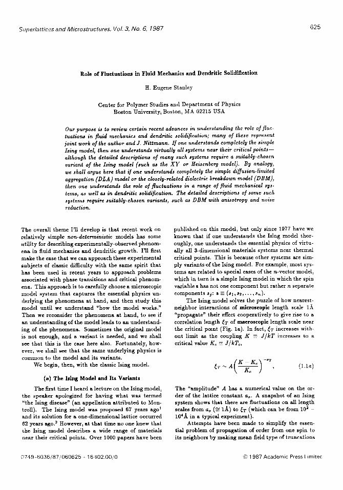
Role of Fluctuations in Fluid Mechanics and Dendritic Solidification

Srrperlattices and Microstructures, Vol. 3, No. 6, 1987 625

Role of Fluctuations in Fluid Mechanics and Dendritic Solidification

H. Eugene Stanley

Center for Polymer Studies and Department of Physics Boston University, Boston, MA 02215 USA

Our purpose is to review certain recent advances in understanding the role of flue- tuations in fluid mechanics and dendritic solidification; many of these represent joint work of the author and J. Nittmann. If one understands completely the simple Ising model, then one understands virtually all systems near their critical points- although the detailed descriptions of many such systems require a suitably-chosen variant of the Ising model (such as the XY or Keisenberg model). By analogy, we shall argue here that if one understands completely the simple diffusion-limited aggregation (DLA) model OP the closely-Elated dielectric breakdown model (DBM), then one understands the role of fluctuations in a range of fluid mechanical systems, as well as in dendn’tic solidification. The detailed descriptions of some such systems require suitably-chosen variants, such as DBM with anisotropy and noise reduction.

The overah theme I’ll develop is that recent work on relatively simple non-deterministic models has some utility for describing experimentally-observed phenomena in fluid mechanics and dendritic growth. I’ll first make the case that we can approach these experimental subjects of classic difficulty with the same spirit that has been used in recent years to approach problems associated with phase transitions and critical phenomena. This approach is to carefully choose a microscopic model system that captures the essential physics underlying the phenomena at hand, and then study this model until we understand “how the model works.” Then we reconsider the phenomena at hand, to see if an understanding of the model leads to an understanding of the phenomena. Sometimes the original model is not enough, and a variant is needed, and we shall see that this is the case here also. Fortunately, however, we shall see that the same underlying physics is common to the model and its variants.

We begin, then, with the classic Ising model.

(a) The Is;19 Model and Its Variants

The first time I heard a lecture on the Ising model, the speaker apologized for having what was termed “the Ising disease” (an appellation attributed to Mon- troll). The Ising model was proposed 67 years ago’ and its solution for a one-dimensional lattice occurred 62 years ago.2 However, at that time no one knew that the Ising model describes a wide range of materials near their critical points. Over 1000 papers have been

published on this model, but only since 1977 have we known that if one understands the Ising model thor- oughly, one understands the essential physics of virtually all 3-dimensional materials systems near thermal critical points. This is because other systems are simply variants of the Ising model. For example, most systems are related to special cases of the n-vector model, which in turn is a simple Ising model in which the spin variable s has not one component but rather n separate components Sj: SE (d1,52,...,d,).

The Ising model solves the puzzle of how nearest- neighbor interactions of microscopic length scale IA “propagate” their effect cooperatively to give rise to a correlation length [T of macroscopic length scale near the critical pomt (Fig. la). In fact, (T increases without limit as the coupling K E J/kT increases to a critical value KC E J/kT,,

(l.la)

The “amplitude” A has a numerical value on the order of the lattice constant a,. A snapshot of an Ising system shows that there are fluctuations on all length scales from a, (g IA) to [T (which can be from lo2 - 1O’A in a typical experiment).

Attempts have been made to simplify the essential problem of propagation of order from one spin to its neighbors by making mean-field type of truncations

@749 -6036/87/060625 -+ 16 SO2.00/0 0 1987 Academic Press Llmltec

626 Superlattices and Microstructures, Vol 3, No 6, 7987

(c) s?2 tL- (6)-“’ L

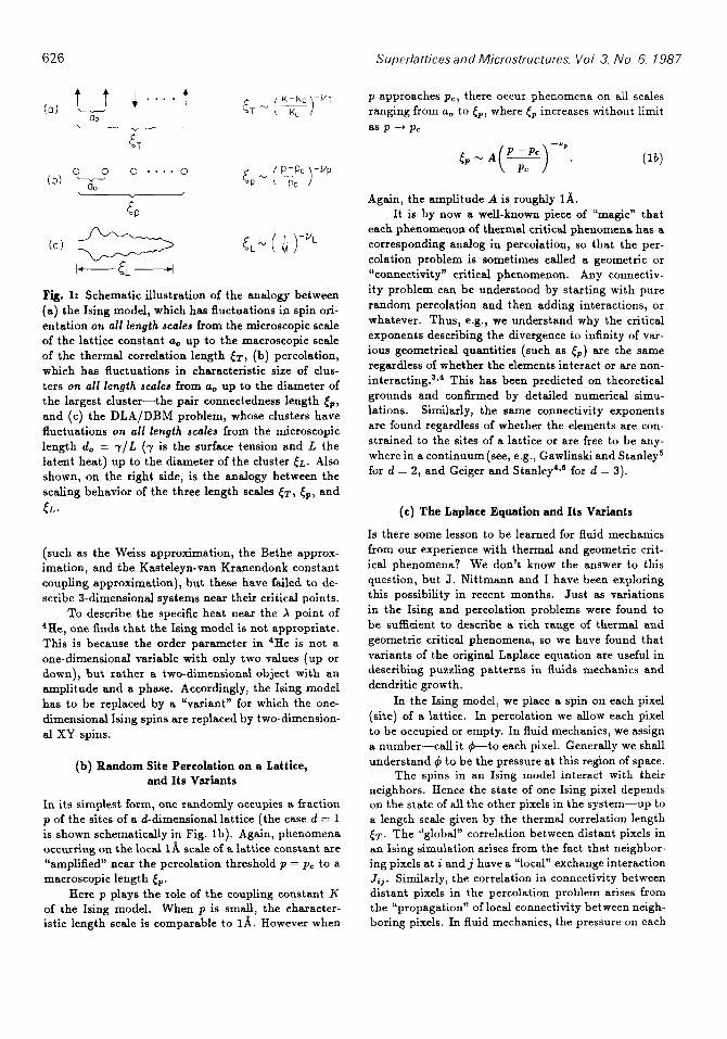
Fig. 1: Schematic illustration of the analogy between (a) the Ising model, which has fluctuations in spin ori- entation on all length scales from the microscopic scale of the lattice constant a, up to the macroscopic scale of the thermal correlation length <T, (b) percolation, which has fluctuations in characteristic size of clusters on all length scales from a, up to the diameter of the largest cluster-the pair connectedness length Q, and (c) the DLA/DBM problem, whose clusters have fluctuations on all length scaled from the microscopic length d, = -y/L (7 is the surface tension and L the latent heat) up to the diameter of the cluster EL. Also shown, on the right side, is the analogy between the scaling behavior of the three length scales (T, &,, and CYL.

(such as the Weiss approximation, the Bethe approximation, and the Kasteleyn-van Kranendonk constant coupling approximation), but these have failed to describe 3-dimensional systems near their critical points.

To describe the specific heat near the A point of 4He, one finds that the Ising model is not appropriate. This is because the order parameter in 4He is not a one-dimensional variable with only two values (up or down), but rather a two-dimensional object with an amplitude and a phase. Accordingly, the Ising model has to be replaced by a “variant” for which the one- dimensional Ising spins are replaced by two-dimensional XY spins.

(b) Random Site Percolation on a Lattice, and Its Variants

In its simplest form, one randomly occupies a fraction p of the sites of a d-dimensional lattice (the case d = 1 is shown schematically in Fig. lb). Again, phenomena occurring on the local 18, scale of a lattice constant are “amplified” near the percolation threshold p = p, to a macroscopic length &,.

Here p plays the role of the coupling constant K of the Ising model. When p is small, the characteristic length scale is comparable to 1A. However when

p approaches p,, there occur phenomena on all scales ranging from a, to tP, where tP increases without limit as P ---t pe

Again, the amplitude A is roughly 1A. It is by now a well-known piece of “magic” that

each phenomenon of thermal critical phenomena has a corresponding analog in percolation, so that the percolation problem is sometimes called a geometric or “connectivity” critical phenomenon. Any connectivity problem can be understood by starting with pure random percolation and then adding interactions, or whatever. Thus, e.g., we understand why the critical exponents describing the divergence to infinity of various geometrical quantities (such as &,) are the same regardless of whether the elements interact or are non- interacting. ‘v4 This has been predicted on theoretical grounds and confirmed by detailed numerical simulations. Similarly, the same connectivity exponents are found regardless of whether the elements are con- strained to the sites of a lattice or are free to be any- where in a continuum (see, e.g., Gawlinski and Stanley5 for d = 2, and Geiger and Stanley4%s for d = 3).

(c) The Laplace Equation and Its Variants

Is there some lesson to be learned for fluid mechanics from our experience with thermal and geometric critical phenomena? We don’t know the answer to this question, but J. Nittmann and I have been exploring this possibility in recent months. Just as variations in the Ising and percolation problems were found to be sufficient to describe a rich range of thermal and geometric critical phenomena, so we have found that variants of the original Laplace equation are useful in describing puzzling patterns in fluids mechanics and dendritic growth.

In the Ising model, we place a spin on each pixel (site) of a lattice. In percolation we allow each pixel to be occupied or empty. In fluid mechanics, we assign a number-call it d-to each pixel. Generally we shall understand 4 to be the pressure at this region of space.

The spins in an Ising model interact with their neighbors. Hence the state of one Ising pixel depends on the state of all the other pixels in the system-up to a length scale given by the thermal correlation length IT. The “global” correlation between distant pixels in an Ising simulation arises from the fact that neighbor- ing pixels at i and j have a “local” exchange interaction Jij. Similarly, the correlation in connectivity between distant pixels in the percolation problem arises from the “propagation” of local connectivity between neigh- boring pixels. In fluid mechanics, the pressure on each

Superlattices and Microstructures, Vol. 3, No. 6, 1987 627

pixel is correlated with the pressure at every other pixel because the pressure obeys the Laplace equation.

One can calculate an equilibrium Ising configuration by “passing through the system with a computer” and flipping each spin with a probability related to the Boltzmann factor. Similarly, one can calculate the pressure at each pixel by “passing through the system” and re-adjusting the pressure on each pixel in accord with the Laplace equation.* If we were to arbitrarily flip the configuration of a single pixel in the Ising problem (from +l to -l), we would significantly influence the equilibrium configuration of the system out to a length scale on the order of <T. Similarly, if we were to arbitrarily impose a given pressure on a single point of a system obeying the Laplace equation, we would drastically change the resulting pattern out to a length scale that we shall call EL.

Does [r; obey a “scaling form” analogous to (la) and (lb) obeyed by the functions [T and Q for the Ising model and percolation? We believe that the answer to this question is “yes,” although our ideas on this subject remain somewhat tentative and subject to revision.

The best way to see the fluctuations inherent in structures grown according to the Laplace equation is to first introduce some specific models. There are two models that were at once thought to be fully equivalent, although it is now recognized that the actual patterns produced by each have a different “susceptibility to lattice anisotropy.” The first of these models is diffusion limited aggregation (DLA). Here one releases a random walker from a large circle surrounding a seed particle placed at the origin. When the random walker touches a perimeter site of the seed, it “sticks” (i.e., the perimeter site becomes a cluster site), and we have a cluster of mass = 2. A second random walker is then released. This process continues until a large cluster is formed. Initially the “mass” M of clusters was typically lo3 to 104. However it has become possible to make very fast algorithms, and the largest cluster to date has a mass of 4 x 1os.s

The second of the two, the dielectric breakdown model (DBM), differs from DLA in that nothing hap- pens until the random walker touches a cluster site, at which time the perimeter site it was just on at the previous step is transformed into a cluster site. Not surprisingly, this tiny local change in boundary conditions does not affect the “critical exponents” of this problem-DLA and DBM have the same value of the fractal dimension df describing how the cluster mass

* There is an intimate connection between the diffusion equation and the random walk problem (see, e.g., Chandrasekhar.‘)

depends on cluster diameter L: M - Ldt.t In both thermal critical phenomena (or percolation) the length L introduced when we have a finite system siee scales the same as the correlation lengths (T (or &,). Hence for DLA we expect that there will be fluctuations on length scales up to [L, where (L itself increases with the cluster mass according to

-“l. [VL = l/df]. (Ic)

Here the amplitude A is again on the order of IA. Note that (lc) is analogous to (la) and (lb) if we think of M -+ 00 as being analogous to K -+ Kc. This reason- ing is common in polymer physics, where we relate the radius of gyration R, of a polymer to the mass through an equation of the form of (lc), R, - (l/M)-‘/dl. Note that or, = l/df plays the role of the critical exponents VT and up of (la) and (lb). Suppose we test this idea, qualitatively, by examining the largest DLA clusters in detail. We find that indeed there are fluctuations in mass on length scales less than, say, the width W of the side branches. If one makes a log-log plot of W against mass M, one finds the same slope l/df that one finds when one plots the diameter against M.

Evidence for Similarity of Viicoua Fingering Patterm and Laplace Equation (DLA/DBM) Patterns

In the remainder of this talk, we’ll describe in some detail the sorts of results we obtain from variants of the Laplaee equation. First, it is necessary to describe the simplest system that produces patterns resembling interesting objects found in nature. Consider, e.g., the classic SafFman-Taylor viscous fingering problem. Here one injects a low-viscosity fluid into a medium tilled with high viscosity fluid. In the limit that the viscosity ratio between the high and low viscosity fluids

t The difference in boundary conditions doea affect the rate at which the asymptotic behavior shows up.? For example, for DLA the screening will be more se- vere: as soon as a random walker steps on a perimeter site, the walker is stopped and the perimeter site becomes a cluster site. However for the DBM a random walker is free to walk on perimeter sites with im- punity: only when the walker steps on a cluster site does the walker stop walking. Hence in the DBM the walkers can better penetrate the fjords of the system, so in overall appearance DBM clusters appear to have thicker branches and to be more “compact.” The critical exponent VL = l/df is not changed since it depends not on the density but on the rate at which the density decreases as the mass increases.

628 Superlattices and Microstructures, Vol 3. No 6. I Yf3

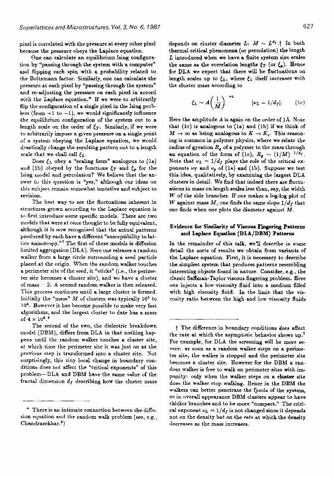
Fig. 2: Schematic illustration of the lateral and radial Hele-Shaw cells. Shown are top views. The spacing between the plates is typically 1 mm or less. From Daccord et al.‘s

can be taken to be zero, we can assume that the pressure everywhere inside the low viscosity fluid is a constant: P(i) = 1 for i E [cluster of pixels occupied by low-viscosity fluid]. The pressure everywhere else in the system will have a value given by the solution of the Laplace equation. This problem is modelled by the dielectric breakdown model or DBM” or diffusion- limited aggregation model or DLA.” These two models have in common that both are solutions to Laplsce equation for the case in which the pressure is zero at infinity and P = 1 on an object called the cluster.

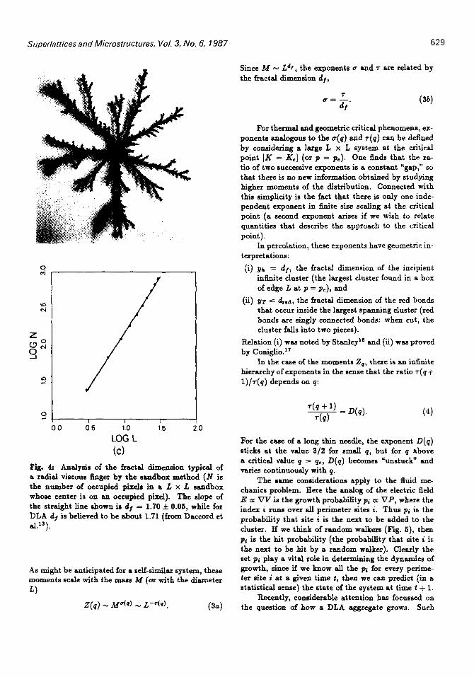
Daccord has made accurate measurements on the fractal dimension of viscous fingers in both laterall and radial13 geometries (Fig. 2). He reduced the length scale normally imposed by surface tension by using liq- uids with zero interfacial tension-the two fluids were water and a viscous aqueous solution of polysaccharide (Fig. 3). He found that the resulting patterns are indeed fractal, with a fractal dimension identical to that of DLA/DBM (Fig. 4). M&y et al” found analogous behavior where the cell itself introduced the randomness: he accomplished this by placing glass beads inside the cell at random. Chen and Wilkinson15 imposed the randomness by studying viscous fingering inside a network of glass tubes whose diameter L was randomly chosen from a probability distribution x(L).

Not only is the fractal dimension the same for the fluid mechanics problem and for the Laplace patterns, but so also are the multifractal propertier the same.

i_ - c

Fig. ): The growth region of a radial viscous finger, a typical experimental pattern for which DLA is the appropriate model. The finger at time 1 = t. is shown in (a), while (b) displays the difference between the pattern at t = t+At and t = t, obtained experimentally by simply subtracting the images of the same finger photographed at slightly different times. After Daccord et al.‘r

Multifractals arise when one defines some quantity on all the pixel sites. Perhaps the simplest example is that of a charged needle: if we assign to every pixel a number equal to the electric field, then the set {Hi} of field values for the perimeter sites of the needle form a multifractal set. The distribution n(E) giving the number of perimeter pixels with electric field E is characterized, like all distribution functions, by its moments

Z(q) = c n(E)E’. E


z W2

3

U-J i

0.0 0.5 1.0 1.5 2.0

LOG L (c)

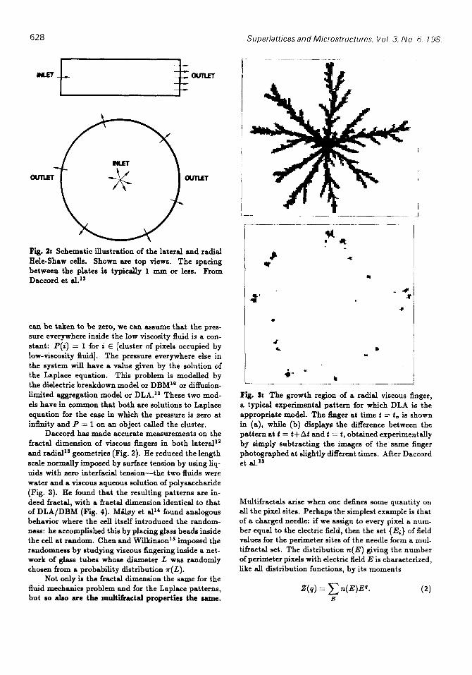
Fig. 4: Analysis of the fractal dimeneion typical of a radial viscous Snger by the sandbox method (N is the number of occupied pixela in a L x L sandbox whose center is on an occupied pixel). The slope of

the straight line rhown ir df = 1.70 f 0.05, while for DLA df is believed to be about 1.71 (from Daccord et al.i3).

As might be anticipated for a self-similar system, these moments scale with the ma88 M (or with the diameter

L)

Z(q) N A&‘) ‘v L-+1. (34

Since M - Ldt, the exponents u and T are related by the fract al dimension df ,

OZZ. d f

WI

For thermal and geometric critical phenomena, exponents analogous to the o(q) and t(q) can be defined by considering a large L x L system at the critical point [K = K,] (or p = pc). One finds that the ratio of two successive exponents is a constant Ugap,” 50 that there is no new information obtained by studying higher moments of the distribution. Connected with this simplicity is the fact that there is only one independent exponent in fmite size scaling at the critical point (a second exponent arises if we wish to relate quantities that describe the approach to the critical point).

In percolation, these exponents have geometric in- terpretations:

(i) y5 = df, the fractal dimension of the incipient infinite cluster (the largest cluster found in a box of edge L at p = pC), and

(ii) YT = dvedr the fractal dimension of the red bonds that occur inside the largest spanning cluster (red bonds are singly connected bonds: when cut, the cluster falls into two pieces).

Relation (i) was noted by Stanley”’ and (ii) was proved by Coniglio.”

In the case of the moments Z,, there is an in&-rite hierarchy of exponents in the sense that the ratio r(q + 1)/r(q) depends on q:

For the cese of a long thin needle, the exponent D(q) sticka at the value 3/2 for small q, but for q above a critical value q = qc, D(q) becomes “unstuck” and varies continuously with q.

The same consideration5 apply to the fluid mechanics problem. Here the analog of the electric field E 0: V1/ is the growth probability pi EL: VP, where the index i runs over all perimeter sites i. Thus pi is the probability that site i is the next to be added to the cluster. If we think of random walker5 (Fig. 5), then pi is the hit probability (the probability that site i is the next to be hit by a random walker). Clearly the set pi play a vital role in determining the dynamics of growth, since if we know all the pi for every perime ter site i at a given time t, then we can predict (in a statistical sense) the state of the system at time t + 1.

Recently, considerable attention has focussed OIL the question of how a DLA aggregate grows. Such

630 Superlattices and Microstructures. Vol. 3, No. 6. 1987

‘ ??

850 DIAMETERS

I I ‘ ??

850 DIAMETERS

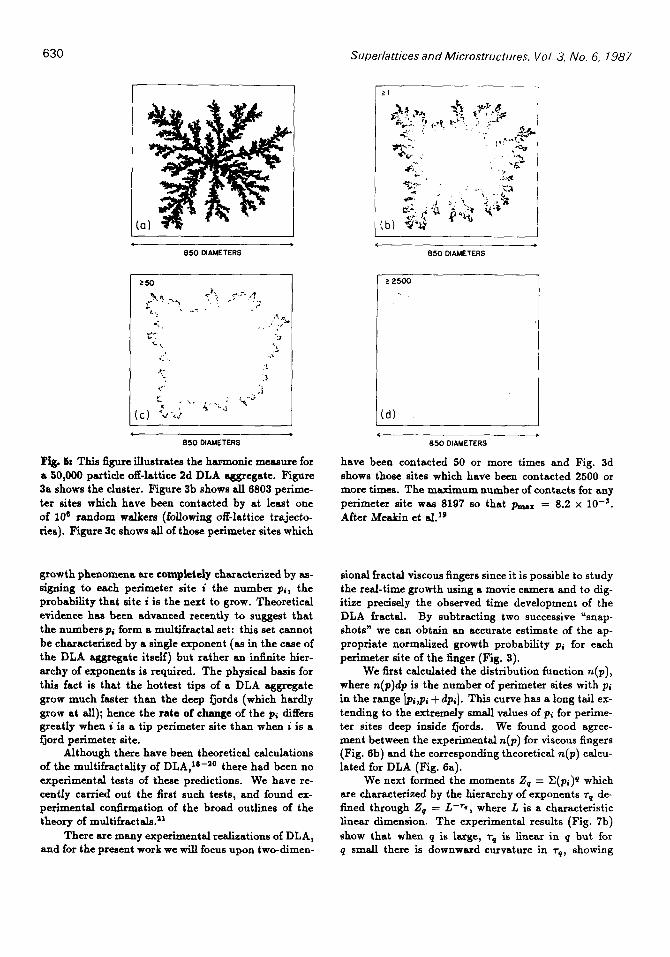
Fig. 6: This figure illustrates the hazmonic measure for a 60,000 particle off-lattice 2d DLA aggregate. Figure 3a shows the cluster. Figure 3b shows zU6803 perimeter sites which have been contacted by at least one of 10” random walkers (following off-lattice trajectories). Figure 3c shows all of those perimeter sites which

growth phenomena are completely characterized by as- signing to each perimeter site i the number pi, the probability that site i is the next to grow. Theoretical evidence has been advanced recently to suggest that the numbers pi form a multifractal set: this set cannot be characterized by a single exponent (as in the case of the DLA aggregate itself) but rather an infinite hierarchy of exponents is required. The physical basis for this fact is that the hottest tips of a DLA aggregate grow much faster than the deep fjords (which hardly grow at all); hence the rate of change of the pi differs greatly when i is a tip perimeter site than when i is a fjord perimeter site.

Although there have been theoretical calculations of the multifiactality of DLA,‘s-so there had been no experimental tests of these predictions. We have recently carried out the first such tests, and found experimental confirmation of the broad outlines of the theory of multikactals.”

There are many experimental realizations of DLA, and for the present work we will focus upon two-dimen-

850 DIAMETERS

z 2500

850 DIAMETERS

have been contacted 50 or more times and Fig. 3d shows those sites which have been contacted 2500 or more times. The maximum number of contacts for any perimeter site was 8197 so that p,_= = 8.2 x 10V3. After Meakin et al.r9

sional fractal viscous fingers since it is possible to study the real-time growth using a movie camera and to dig- itize precisely the observed time development of the DLA fractal. By subtracting two successive “snap- shots” we can obtain an accurate estimate of the appropriate normalized growth probability pi for each perimeter site of the finger (Fig. 3).

We first calculated the distribution function n(p), where n(p)dp is the number of perimeter sites with pi in the range [pi,pi + dpi]. This curve has a long tail ex- tending to the extremely small values of pi for perimeter sites deep inside fjords. We found good agree- ment between the experimental n(p) for viscous fingers (Fig. 6b) and the corresponding theoretical n(p) calculated for DLA (Fig. 6a).

We next formed the moments 2, = II( which are characterized by the hierarchy of exponents r, defined through 2, = L-Q, where L is a characteristic linear dimension. The experimental results (Fig. 7b) show that when 9 is huge, rq is linear in p but for 4 small there is downward curvature in rq, showing

Superlattices and Microstructure.% Vol. 3, NO. 6, 1987 631

h P

(a) Fll. 6: Comparison between the distribution functions n(p) for simulated (a) and “experimental” (b) viscous fingering patterns. Here n(p)6p is the number of perimeter sites with growth probabilities in the range [p,p + 6~1. The simulated patterns and their growth probabilities were obtained using the dielectric breakdown model. The growth probabilities for the ezperi- mental patterns were obtained by numerically solving

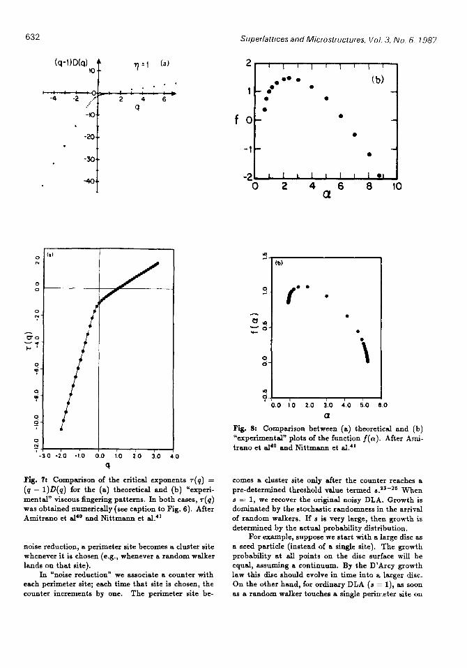
that the fjords are characterized by different growth rates than the tips. It is conventional to also CI&X- late the Legendre transform with respect to q of 7s: -f(a) = T(q) - qu where a = h/dq. Downward curvature in T(q) corresponds to upward curvature in -f(a) [Fig. 8a]. The experimental data of Figs. 7b and gb compare favorably with the theoretical DLA model calculations shown in Figs. ?a and 8s.

UDendritic SoliditIcation~ Variants of the Fluid Mcchanlcal Models

By analogy with the Ising model and its variants, we can modify DLA/DBM to describe other fluid mechanical phenomena. One of the most intriguing of these is a variation of the viscous fingering phenomenon in which there is present anisotropy. Ben Jacob et alla imposed this anisotropy by scratching a lattice of lines on their Hele-Shaw cell. They found patterns that strongly resemble snow crystals! If viscous fingers are described by DLA, then can the Ben Jacob patterns be described by DLA with imposed anisotropy?

Nittmann and Stanley’s attempted to answer this question-specifically, they attempted to reproduce the Ben Jacob patterns with suitably modified DLA. A scratch in a Hele-Shaw cell means that the plate spacing b is increased along certain directions, and the per- meability coefficient k relating growth velocity to VP

LO -a0 -I2 0 -16 0 -200 Cn P

(h)

the Laplsce equation in the vicinity of a digitized repre- sentation of the pattern with absorbing boundary conditions on the sites occupied by the pattern. Similar results were obtained for large a (corresponding to the “tips”) by directly subtracting two successive experimental patterns. After Amitrano et al’O and Nittmann et al.”

is proportional to b”(k ac U). Hence Nittmann and Stanley calculated DLA patterns for the case in which there was imposed a periodic variation in the k. It is significant that their simulations reproduce snow crystal type patterns, just like the experiments. These simulations relied for their e&acy on the presence of noise reduction.

Noise Reduction

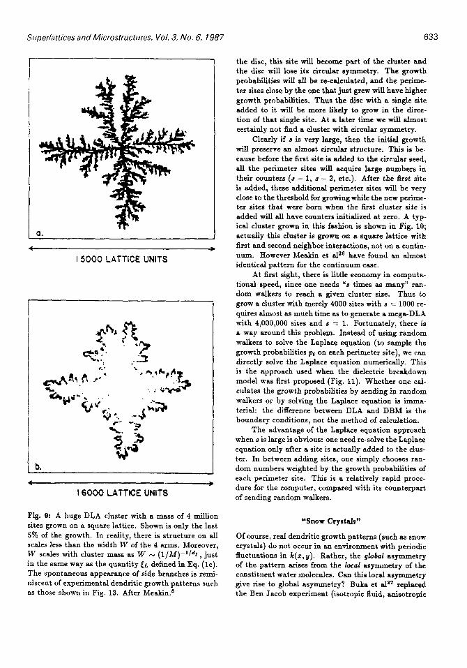
The original DLA and DBM models are prototypes of completely chaotic systems. No discernable pattern emerges. If there is a weak anisotropy, we expect that the resulting pattern reflects this anisotropy. For example, if the simulations are carried out on a lattice, then the presence of the lattice imposes a weak anisotropy (e.g., on a square lattice, it is more likely that particles attach to the westernmost tip if they approach from the west than from the north or south). This weak anisotropy is not visually apparent unless large clusters are grown. However the largest DLA clusters made’ with mass about 4 million sites, clearly display the anisotropy (Fig. 9). Unfortunately, no one can afIord the computer resources to make such “mega- DLA” clusters each time we wish to model a new phenomenon. Noise reduction is a computational trick that seems to have the property that it speeds up the attainment of this asymptotic limit. In the absence of

632 Superlattices and Microstructures, Vol. 3, No. 6, 7.987

(q-l ID(q) ,. 7 L 1 (a) 2. , , , , , , , , , 1

??e. 0 (b) 1 - f a

0 0

f 0-O a 0

. * * . * ??

2 4 6

I,.. 9

.

-20.. .

-30..

-40..

Pig. 7: Comparison of the critical exponents T(q) = (q - l)D(q) for the (a) theoretical and (b) “experimental” viscous fingering patterns. In both cases, s(q) was obtained numerically (see caption to Fig. 6). After Amitrano et al”’ and Nittmann et al.”

noise reduction, a perimeter site becomes a cluster site whenever it is chosen (e.g., whenever a random walker lands on that site).

In “noise reduction” we associate a counter with each perimeter site; each time that site is chosen, the counter increments by one. The perimeter site be-

-1 - 0

-2‘ 1 1 I I I I I I .I

0 2 4 6 8 10 a

b)

I . .

??

.

. .

\

0.0 1.0 2.0 3.0 4.0 5.0

a

.O

k’lg. 8: Comparison between (a) theoretical and (b) “experimental” plots of the function f(o). After Ami- trano et al”O and Nittmann et a14r

comes a cluster site only after the counter reaches a pre-determined threshold value termed s.s3-25 When 8 = 1, we recover the original noisy DLA. Growth is dominated by the stochastic randomness in the arrival of random walkers. If s is very large, then growth is determined by the actual probability distribution.

For example, suppose we start with a large disc as a seed particle (instead of a single site). The growth probability at all points on the disc surface will be equal, assuming a continuum. By the D’Arcy growth law this disc should evolve in time into a larger disc. On the other hand, for ordinary DLA (s = l), as soon as a random walker touches a single perirr.eter site on

Superlattices and Microstructures, Vol. 3, No. 6, 1987

I5000 LATTICE UNITS

b.

- I SCM20 LATTICE UNITS

k’lg. 9: A huge DLA cluster with a mass of 4 million sites grown on a square lattice. Shown is only the last 5% of the growth. In reality, there is structure on all scales less than the width W of the 4 arms. Moreover, W scales with cluster mass as W - (l/i~I-‘/~l, just in the same way as the quantity [r. defined in Eq. (1~). The spontaneous appearance of side branches is remi- niscent of experimental dendritic growth patterns such as those shown in Fig. 13. After Meakin.*

633

the disc, this site will become part of the cluster and the disc will lose its circular symmetry. The growth probabilities will all be re-calculated, and the perimeter sites close by the one that just grew will have higher growth probabilities. Thus the disc with a single site added to it will be more likely to grow in the direction of that single site. At a later time we will almost certainly not find a cluster with circular symmetry.

Clearly if s is very large, then the initial growth will preserve an almost circular structure. This is because before the first site is added to the circular seed, all the perimeter sites will acquire large numbers in their counters (8 - 1, B - 2, etc.). After the first site is added, these additional perimeter sites will be very close to the threshold for growing while the new perimeter sites that were born when the first cluster site is added will all have counters initialized at zero. A typical cluster grown in this fashion is shown in Fig. 10; actually this cluster is grown on a square lattice with first and second neighbor interactions, not on a continuum. However Meakin et alzE have found an almost identical pattern for the continuum case.

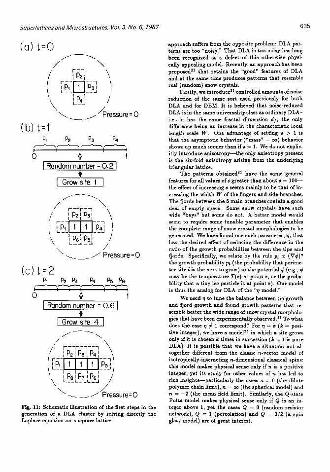
At first sight, there is little economy in computational speed, since one needs =a times as many” random walkers to reach a given cluster size. Thus to grow a cluster with merely 4000 sites with s = 1000 re- quires almost as much time as to generate a mega-DLA with 4,000,OOO sites and s = 1. Fortunately, there is a way around this problem. Instead of using random walkers to solve the Laplace equation (to sample the growth probabilities pi on each perimeter site), we can directly solve the Laplace equation numerically. This is the approach used when the dielectric breakdown model was first proposed (Fig. 11). Whether one cal- culates the growth probabilities by sending in random walkers or by solving the Laplace equation is imma- terial: the difference between DLA and DBM is the boundary conditions, not the method of calculation.

The advantage of the Laplace equation approach when s is large is obvious: one need re-solve the Laplace equation only after a site is actually added to the cluster. In between adding sites, one simply chooses random numbers weighted by the growth probabilities of each perimeter site. This is a relatively rapid proce- dure for the computer, compared with its counterpart of sending random walkers.

“Snow Crystals”

Of course, real dendritic growth patterns (such as snow crystals) do not occur in an environment with periodic fluctuations in k(z,y). Rather, the global asymmetry of the pattern arises from the local asymmetry of the constituent water molecules. Can this local asymmetry give rise to global asymmetry? B&a et als’ replaced the Ben Jacob experiment (isotropic fluid, anisotropic

634 Superlattices and Microstructures, Vol. 3. No. 6, 1987

cell) by the reverse: isotropic cell but anisotropic fluid! To accomplish this, they used a nematic liquid crystal for the high viscosity fluid. Thus the analog of the water molecules in a snow crystal are the rod-shaped anisotropic molecules of a nematic. This experiment shows that the underlying anisotropy can as well be in the fluid as in the environment.

Snow crystal formation is thought to be mainly the aggregation of tiny ice particles and droplets of su- percooled water. To the extent that snow crystals grow by accreting water molecules previously in the vapor or liquid phase, the growth rate is thought to be limited by the diffusion away from the growing snow crystal of the latent heat released by these phase changes. Under conditions of small Peclet number, the diffusion equation describing the space and time dependence of the temperature field T(r,t) reduces to the Laplace equation. Thus a reasonable starting point is DLA, independent of whether we wish to focus on particle aggregation, heat diffusion, or both.

DLA reflects well the randomness inherent in a wide range of growth processes, including colloidal aggregation, it fails to describe dendritic solidification. While the deterministic models of snow crystals pro- duce patterns that are much too “symmetric,” the DLA

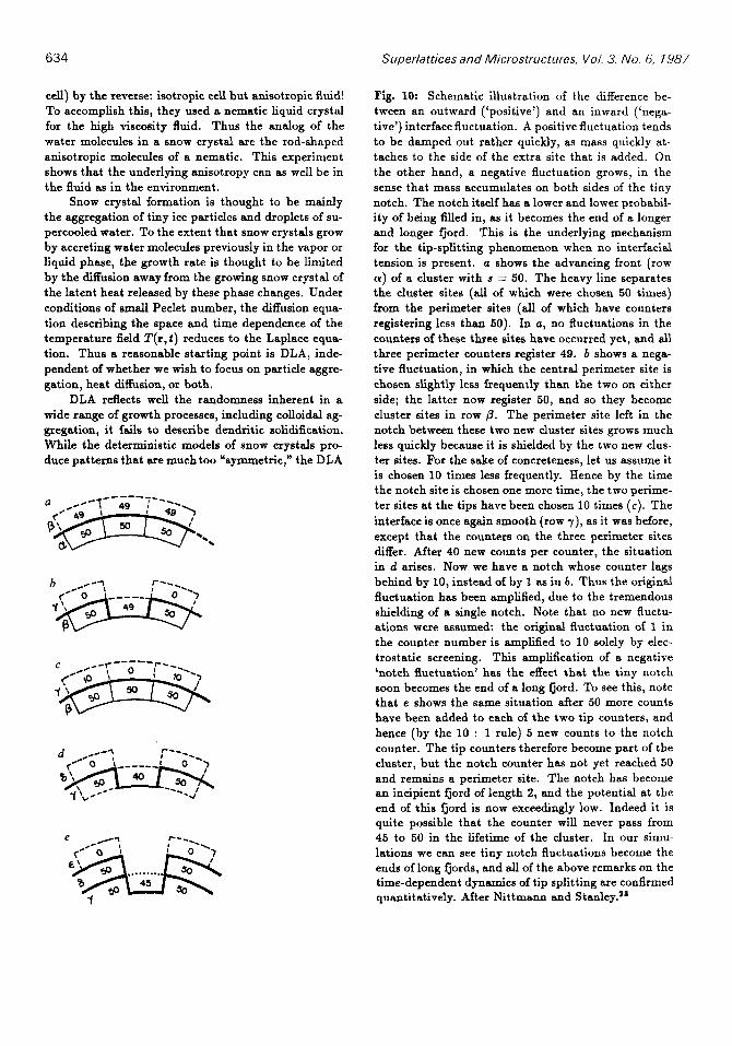
Fig. 10: Schematic illustration of the difference between an outward (‘positive’) and an inward (‘negative’) interface fluctuation. A positive fluctuation tends to be damped out rather quickly, as mass quickly at- taches to the side of the extra site that is added. On the other hand, a negative fluctuation grows, in the sense that mass accumulates on both sides of the tiny notch. The notch itself has a lower and lower probability of being filled in, as it becomes the end of a longer and longer fjord. This is the underlying mechanism for the tip-splitting phenomenon when no interfacial tension is present. a shows the advancing front (row a) of a cluster with a = 50. The heavy line separates the cluster sites (all of which were chosen 50 times) from the perimeter sites (all of which have counters registering less than 50). In a, no fluctuations in the counters of these three. sites have occurred yet, and all three perimeter counters register 49. b shows a negative fluctuation, in which the central perimeter site is chosen slightly less frequently than the two on either side; the latter now register 50, and so they become cluster sites in row /3. The perimeter site left in the notch between these two new cluster sites grows much less quickly because it is shielded by the two new cluster sites. For the sake of concreteness, let us assume it is chosen 10 times less frequently. Hence by the time the notch site is chosen one more time, the two perimeter sites at the tips have been chosen 10 times (c). The interface is once again smooth (row T), as it was before, except that the counters on the three perimeter sites differ. After 40 new counts per counter, the situation in d arises. Now we have a notch whose counter lags behind by 10, instead of by 1 ss in b. Thus the original fluctuation has been amplified, due to the tremendous shielding of a single notch. Note that no new fluctuations were assumed: the original fluctuation of 1 in the counter number is amplified to 10 solely by electrostatic screening. This amplification of a negative ‘notch fluctuation’ has the effect that the tiny notch soon becomes the end of a long fjord. To see this, note that e shows the same situation after 50 more counts have been added to each of the two tip counters, and hence (by the 10 : 1 rule) 5 new counts to the notch counter. The tip counters therefore become part of the cluster, but the notch counter has not yet reached 50 and remains a perimeter site. The notch has become an incipient fjord of length 2, and the potential at the end of this fjord is now exceedingly low. Indeed it is quite possible that the counter will never pass from 45 to 50 in the lifetime of the cluster. In our simulations we can see tiny notch fluctuations become the ends of long fjords, and all of the above remarks on the time-dependent dynamics of tip splitting are confirmed quantitatively. After Nittmann and Stanley.s3


(a) t=O

(

/y-/l \

$-/?+F< 1 I

\ ’ P,l L-J /

\-

/ , Pressure = 0

(b) t=l 4 ?? p3 p4

A-A- I I

0 0 1 Random number = 0.2 ]

9 1 Grow site 1 ]

I

\ \.- / Pressure = 0

Cc) t=2 PI p2 @i p4 p5 p6

-n--h& I 1

0 0 1 Random number = 0.6 ]

1

/ -1

/ \

r-i--i--i \

\ -.- _//Pressure=0

Fig. 11: Schematic illustration of the first steps in the generation of a DLA cluster by solving directly the Laplace equation on a square lattice.

635

approach suffers from the opposite problem: DLA patterns are too “noisy.” That DLA is too noisy has long been recognized as a defect of this otherwise physi- cally appealing model. Recently, an approach has been proposeda that retains the “good” features of DLA and at the same time produces patterns that resemble real (random) snow crystals.

Firstly, we introduces’ controlled amounts of noise reduction of the same sort used previously for both DLA and for DBM. It is believed that noise-reduced DLA is in the same universality class as ordinary DLA- i.e., it has the same fractal dimension df, the only difference being an increase in the characteristic local length scale W. One advantage of setting 8 > 1 is that the asymptotic behavior (“mass” = m) behavior shows up much sooner than if s = 1. We do not explic- itly introduce anisotropy-the only anisotropy present is the six-fold anisotropy arising from the underlying triangular lattice.

The patterns obtained2’ have the same general features for all values of a greater than about s = lOO- the effect of increasing s seems mainly to be that of increasing the width W of the fingers and side branches. The fjords between the 6 main branches contain a good deal of empty space. Some snow crystals have such wide “bays” but some do not. A better model would seem to require some tunable parameter that enables the complete range of snow crystal morphologies to be generated. We have found one such parameter, 7, that has the desired effect of reducing the difference in the ratio of the growth probabilities between the tips and fjords. Specifically, we relate by the rule p; o( (04)” the growth probability p; (the probability that perimeter site i is the next to grow) to the potential 4 (e.g., 0 may be the temperature T(r) at point r, or the probability that a tiny ice particle is at point r). Our model is thus the analog for DLA of the “7 model.”

We used q to tune the balance between tip growth and fjord growth and found growth patterns that resemble better the wide range of snow crystal morphologies that have been experimentally observed.sr To what does the case 7 # 1 correspond? For 7 = L (k = positive integer), we have a mode12s in which a site grows only if it is chosen k times in succession (k = 1 is pure DLA). It is possible that we have a situation not al- together different from the classic n-vector model of isotropically-interacting n-dimensional classical spins: this model makes physical sense only if n is a positive integer, yet its study for other values of n has led to rich insights-particularly the cases n = 0 (the dilute polymer chain limit), n = 00 (the spherical model) and TZ = -2 (the mean field limit). Similarly, the Q-state Potts model makes physical sense only if Q is an integer above 1, yet the cases Q = 0 (random resistor network), Q = 1 (percolation) and Q = 3/2 (a spin glass model) are of great interest.

636 Sugerlattices and Microstructures, Vol 3. No fi 798

The fractal dimension df is believed independent of the value of the noise reduction parameter s (s renor- malises the cluster mass). We confirmed this belief. However, we found df does depend on 7. The most re- liable estimates were obtained by first calculating estimates of df for a sequence of increasing cluster masses, and then extrapolating this sequence to infinite cluster mass. Our values for df agreed remarkably well with values we obtained by digitizing photographs of experimentally observed snow crystals. Of course this preliminary study ‘I does not completely “solve” the snow crystal problem:

(i) The initial seed of a snow crystal is almost certainly hexagonal (i.e., quasi-Z-dimensional), since this is the local geometry that water molecules take when they form hexagonal ice Ih. Are DBM-type con- siderations (small growth probability near the center of a plate-like structure) sufficient to explain why a snow crystal remains quasi-2-dimensional as it continues growing? Why does its thickness remain less than its width? It is perhaps appropriate to mention that no adequate explanation has yet been advanced for why a snow crystal remains quasi-2dimensional throughout its growth, despite the fact that the “assembly plant” is certainly 3dimensional. Intuition on this subject stems from experience not only from critical phenomena but also from recent theoretical and experimental work on pattern formation, where it was found that even minute amounts of anisotropy are sufficient to sta- bilize structures of lower effective dimension.

(ii) What are the microscopic mechanisms that give rise to the feature that real snow crystals contain branches (and side branches) which are much more than one molecule thick? Is noise reduction relevant, or is noise reduction merely a “computational trick” that allows one to see the asymptotic form of a DLA cluster using reasonable masses? (E.g., on a square lattice, the same cross-like pattern for a mass of 5,000 sites seen in noise-reduced DLA with a noise-reduction parameter of s = 500 is also seen in ordinary “noisy” DLA (3 = 1) provided the mass is allowed to increase to roughly 5,000,OOO sites! We know that DLA is obtained even if the incoming random walkers have a sticking probability that is less than one. Hence we anticipate that DLA might possibly describe a modest range of phenomena with structural re-arrangement. What is the actual sticking probability for newly arriving water molecules in real snow crystals? Is a value of the sticking probability less than unity sufficient to account for the fact that the arms and sidebranches of real snow crystals have macroscopic thickness.

(iii) Are those real snow crystals which possess relatively compact cores with ramified dressing on their surfaces products of different environments of assembly, or did melting and structural rearrangement take place after formation? Can one mimic the effect of the

changing environments in which a given snow crystal is actually assembled? Do these correspond to varying parameters such as n or 7 in the course of the growth proceaa? To study this effect, we generated patterns with values of TJ and 7 that change during the growth process-e.g., we might choose q < 1 for an initial fraction f of the growth (thereby creating a hexagonal core), and n = 1 thereafter (thereby creating a ramified exterior portion).

(iv) Does the presence in the clouds of a wind whose direction and speed varies randomly (both in time and in space, with characteristic time scales and length scales that are microscopic) imply that the actual trajectories of water molecules and water droplets might more resemble those of some extremely “patho- logical” path than those of a conventional DLA type random walk? We know that the random walk trajectories of DLA correspond exactly to the present electrostatic growth model, the DBM with DLA boundary conditions. What are the trajectories in “real space” corresponding to a choice of the 7 parameter below unity? One can speculate that a Levy flight with tunable fractal dimension may be related to the path of a real ice particle buffeted around in a cloud.

(v) How significant, in practice, is the role played by diffusion of latent heat away from the growing aggregate in determining the actual structure of a snow crystal? We know that this phenomenon is of paramount importance in dendritic growth of crystals from a liquid phase How significant is the role played by the capil- lary length d, = 7/L in vapor phase deposition of water molecules onto a growing snow crystal? (Here L is the latent heat.) An ideal model might encompass both the diffusion of heat away from the snow crystal and the aggregation of particles toward the snow crystal?

(vi) Are real snow crystals sometimes fractal objects? This intriguing question has been the object of considerable discussion in recent years. Our growth patterns are fractal, for all positive values of 7. We found” that the fractal dimension df is independent of the value of the noise reduction parameter s (3 seems to mainly renormalize the cluster mass), but df does /eject depend on 7. We also found that these values for df agreed well with values we obtained by digitizing the corresponding photographs of experimentally observed snow crystals (Fig. 12).

Dendritic Growth of NHaBr

Dendritic crystal growth has been a field of immense recent progress, both experimentally and theoretically. In particular, Dougherty et alz8 have recently made a detailed analysis of stroboscopic photographs, taken at 20 second intervals, of dendritic crystals of NHdBr (Fig. 13a). They have found three surprising results: (i) the sidebranches are non-periodic at any distance


.8-

0” - Model ??0

0

.o 1.0 2.0 3.0 4.0 5.0 l

In L

637

from the tip, with random variations in both phase and amplitude, (ii) sidebranches on opposite sides of the dendrite are essentially uncorrelated, and (iii) the rms sidebranch amplitude is an exponential function of distance from the tip, with no apparent onset threshold distance. Some of these results are apparently at variance with predictions from recent theories.30-“2

How can we understand these new experimental facts? Many existing models reflect the essential physical laws underlying the growth phenomena, but fail to find a tractable mechanism to incorporate the ef- fects of noise on the growth. Growth of a dendrite from solution is controlled by the diffusion of solute to- wards the growing dendrite. In the limit of small Peclet number, the diffusion equation reduces to the Laplace equation (as mentioned above). The Laplace equation for a moving interface (the growing dendrite) brings to mind the diffusion limited aggregation model (DLA). Growth patterns produced by the various DLA simulation algorithms do not resemble dendritic growth patterns: DLA patterns are much too chaotic in appearance. We shall discuss here a related mode133 whose asymptotic structure does resemble the patterns found experimentally-both in broad qualitative features and in quantitative detail, The picture that emerges is one of Laplacian growth, where noise arises from the fact that there are concentration Auctuations in the vicinity of the growing dendrite (these are estimated to be roughly 1105 NHdBr molecules per cubic micron).

Our starting point is the observation that minute amounts of anisotropy become magnified as the mass of a cluster increases. In fact, even the weak anisotropy of the underlying lattice structure can become so amplified that clusters of 4,000,OOO particles take on a cross- like appearance. A real dendrite has a mass of roughly 10” particles; it is impossible to generate clusters of this size on a computer, since even clusters of size lo6 require hundreds of hours on the fastest available com- puters. Fortunately, there is a computational trick--- termed n&e reduction-that speeds the convergence

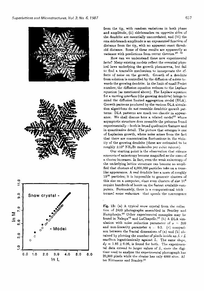
Fig. 12: (a) A typical snow crystal from the collec- tion of 2453 photographs assembled in Bentley and Humphreys. 44 Other experimental exampies may be found in Nakaya42 and LaChapelle.*’ (b) A DLA simulation with noise reduction parameter of s =: 200 and non-linearity parameter n = 0.5. (c) comparison between the fractal dimensions of (a) and (b) obtained by plotting the number of pixels inside an L x L sandbox logarithmically against L. The same slope, dt = 1.85 zb 0.06, is found for both. The experimental data extend to larger values of L, since the digi-

tizer used to analyze the experimental photograph has 20,000 pixels while the cluster has only 4000 sites. Af- ter Nittmann and Stanley?

638

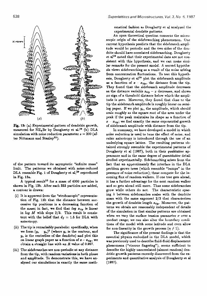
Fig. 13: (a) Experimental pattern of dendritic growth, measured for NHdBr by Dougherty et al.” (b) DLA simulation with noise reduction parameter 8 = 200 (after Nittmann and Stanley33).

of the pattern toward its asymptotic “infinite mass” limit. The patterns we obtained with noise-reduced DLA resemble Fig. 1 of Dougherty et al,” reproduced in Fig. 13a.

A typical result 33 for a mass of 4000 particles is shown in Fig. 13b. After each 333 particles are added, a contour is drawn:

(4

(ii)

It is apparent from the “stroboscopic” representa- tion of Fig. 13b that the distance between successive tip positions is a decreasing function of the mass; in fact, we find that Iog Ztip is linear in Iog M with slope 2/3. This result is consis- tent with the belief that df = 1.5 for DLA with anisotropy.

The tip is remarkably parabolic: specifically, when we form (yC - Y,)~ (where y, is the contour, and y0 is the centerline of the dendrite) and plot this on linear graph paper as a function of z - zkiP, we obtain a straight line with an R value of 0.997.

(iii) The sidebranches are non-periodic at any distance from the tip, with random variations in both phase and amplitude. To demonstrate this, we have analyzed our simulations in exactly the same math-


ematical fashion as Dougherty et al analyzed the experimental dendrite patterns.

An open theoretical question concerns the microscopic origin of the sidebranching phenomenon. One current hypothesis predicts that the sidebranch amplitude would be periodic and the two sides of the dendrite should have correlated sidebranching. Dougherty et al” noted that their experimental data are not con- sistent with this hypothesis, and we can make similar remarks for the present model. A second hypothesis views sidebranching as a result of the noise arising from concentration fluctuations. To test this hypothesis, Dougherty et al” plot the sidebranch amplitude as a function of z - Ztipr the distance from the tip. They found that the sidebranch amplitude decreases as the distance variable ztip - z decreases, and shows no sign of a threshold distance below which the amplitude is zero. Moreover, they found that close to the tip the sidebranch amplitude is roughly linear on semi- log paper. If we plot yC, the amplitude, which should scale roughly as the square root of the area under the peak if the peak maintains its shape as a function of z - Ztip; we find exactly the same exponential growth of sidebranch amplitude with distance from the tip.

In summary, we have developed a model in which noise reduction is used to tune the effect of noise, and cubic anisotropy is introduced through the use of an underlying square lattice. The resulting patterns obtained strongly resemble the experimental patterns of Dougherty et al (1987), both in their qualitative appearance and in the same degree of quantitative detail studied experimentally. Sidebranching arises from the fact that an approximately flat interface in the DLA problem grows trees (which resemble “bumps” in the presence of noise reduction); these compete for the incoming flux of random walkers. If one tree gets ahead, it has a further advantage for the next random walker and so gets ahead still more. Thus some sidebranches grow while others do not. The characteristic spacing A between sidebranches scales with the dendrite mass with the same exponent 2/3 that characterizes the growth of dendrite length Etip. Moreover, the patterns we obtain are reasonably independent of details of the simulation in that similar patterns are obtained when we vary the surface tension parameter (r over a modest range; we can also alter the boundary conditions of the model with some latitude and even allow for non-linearity in the growth process (1 # 1).

The significance of the present findings is that the essential physics embodied in the DLA model, which was previously used to describe fluid-fluid displacement phenomena (“viscous fingering”), seems sufficient to describe the highly uncorrelated (almost random) dendritic growth patterns recently discovered from the experiments and quantitative analysis of Dougherty et al (1987).


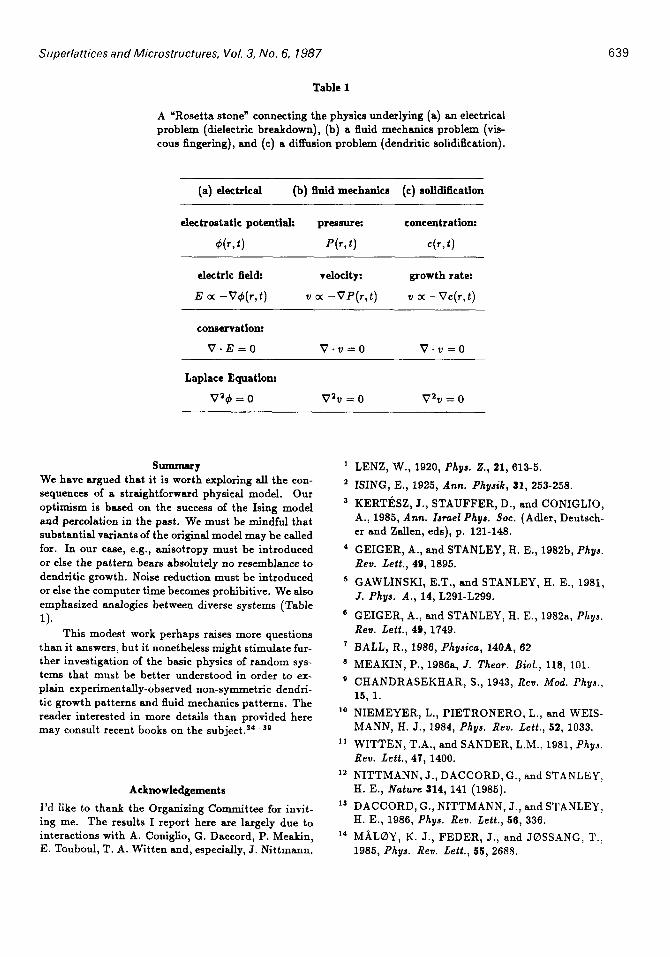
Table 1

A “Rosetta stone” connecting the physice underlying (a) an electrical problem (dielectric breakdown), (b) a fluid mechanics problem (viscous fingering), and (c) a diffusion problem (dendritic solidification).

(a) electrical (b) fluid mechanics (c) solidification

electrostatic potential: pressure: concentration:

4(rr t) P(r, t) c(r, t)

electric field: velocity: growth rate:

E a -V4(r, t) v a -VP(r, t) v a -Vc(r,t)

conservation:

V.E=O v-v=0 v*v=o

Laplace Equation:

VZd=O -7% = 0 v2v = 0

s-r We have argued that it is worth exploring alI the con- sequences of a straightforward physical model. Our optimism is based on the success of the Ising model and percolation in the past. We must be mindful that substantial variants of the original model may be called for. In our case, e.g., anisotropy must be introduced or else the pattern bears 8bsoluteIy no resemblance to dendritic growth. Noise reduction must be introduced or else the computer time becomes prohibitive. We also emphasized analogies between diverse systems (Table

1). This modest work perhaps raises more questions

than it answers, but it nonetheless might stimulate further investigation of the basic physics of random systems that must be better understood in order to explain experimentally-observed non-symmetric dendritic growth patterns and fluid mechanics patterns. The reader interested in more details than provided here may consult recent books on the subject.34-S0

Acknowledgements

I’d like to thank the Organizing Committee for invit- ing me. The results I report here are largely due to interactions with A. Coniglio, G. Daccord, P. Meakin, E. Touboul, T. A. Witten and, especially, J. Nittmann.

LENZ, W., 1920, Phyd. Z., 21, 613-5.

ISING, E., 1925, Ann. Phydik, 31, 253-258.

KERTIkSZ, J., STAUFFER, D., and CONIGLIO, A., 1985, Ann. Israel Phya. Sot. (Adler, Deutsch- er and Zallen, eds), p. 121-148.

GEIGER, A., and STANLEY, H. E., 1982b, Phyd. Rev. Lett., 49, 1895.

GAWLINSKI, E.T., and STANLEY, H. E., 1981, J. Phys. A., 14, L291-L299.

GEIGER, A., and STANLEY, H. E., 19828, Phys. Rev. Lett., 49, 1749.

HALL, R., 1986, Physica, 14liA, 62

MEAKIN, P., 19868, J. Theor. B&l., 118, 101.

CHANDRASEKHAR, S., 1943, Rev. Mod. Phys., 15, 1.

NIEMEYER, L., PIETRONERO, L., and WEIS- MANN, H. J., 1984, Phyr. Rev. Lett., 52, 1033.

WITTEN, T.A., and SANDER, L.M., 1981, Phys. Rev. Lett., 47, 1400.

NITTMANN, J., DACCORD,G., and STANLEY, H. E., Nature 314, 141 (1985).

DACCORD, G., NITTMANN, J., and STANLEY, H. E., 1986, Phys. Rev. Lett., 56, 336.

MALBY, K. J., FEDER, J., and JBSSANG, T., 1985, Phyd. Rev. Lett., 55, 2688.

640 Superlattices and Microstructures, Vol. .X, No 6. 7 98987

15

16

17

1.9

19

21

25

24

25

26

2'1

28

29

30

31

CHEN, J. D. and WILKINSON, D., 1985, Phya. Rev. Lett., 55, 1985.

STANLEY, H. E., 1977, J. Phya. A, 10, LZll- L220.

CONIGLIO, A., 1982, J. Phys. A, 15, 3829.

MEAKIN, P., STANLEY, H. E., CONIGLIO, A., and WITTEN, T. A., 1985, Phyd. Rev. A, 32, 2364.

MEAKIN, P., CONIGLIO, A., STANLEY, H. E., and WITTEN, T. A., 1986, Phyd. Rev. A, 54, 3325-3340.

HALSEY, T. C., MEAKIN, P., and PROCAC- CIA, I., 1986, Phyd. Rev. Lett., 66, 854.

NITTMANN, J., and STANLEY, H. E., 1987a, J. Phyd. A 20, Lxxx.

BEN-JACOB,E., GODBEY,R., GOLDENFELD, N. D., KOPLIK, J., LEVINE, H., MUELLER, T., and SANDER, L. M., 1985, Phya. Rev. Lett., 55, 1315.

NITTMANN, J., and STANLEY, H. E., 1986, Na- ture 321, 663-668.

TANG, C., 1985, Phys. Rev. A., 31, 1977.

KERTkSZ, J., and VICSEK, T., 1986, J. Phya. A, lS, L257.

MEAKIN, P. (et aI) [unpublished].

BUKA, A., KERTIkZ, J., and VICSEK, T., 1986, Nature, 323, 424.

MEAKIN, P., 1986b, Proc. Israel Conference on Fracture.

DOUGHERTY, A., KAPLAN, P. D., and GOL- LUB, J. P., 1987, Phys. Rev. Lett. 58, 1652.

SAITO, Y., GOLDBECK-WOOD, G., and MfiL- LER-KRUMBHAAR, II., 1987, Phya. Rev. Lett., 58, 1541.

BEN-JACOB,E., GOLDENFELD,N., KOTLIAR, B. G., and LANGER, J. S., 1984, Phys. Rev. Lett, 53, 2110.

32

33

34

35

38

31

38

38

40

41

42

43

44

KESSLER, D., KOPLIK, J., and LEVINE, H., 1984, Phys. Rev. A, SO, 3161.

NITTMANN, J., and STANLEY, H. E., 1987h, J. Phys. A 20, Lxxx.

FAMILY, F. and LANDAU, D. P. (eds), 1984, Ki- neticd of Aggregation and Gelation (Elsevier, Am- sterdam).

BOCCARA,N. & DAOUD,M. (eds), 1985, Phydicd of Finely Divided Matter [Proceedings of the Win- ter School, Les Houches, 19851 (Springer Verlag, Heidelberg).

PYNN,R. and SKJELTORP,A. (eds.), 1986, Scal- ing Phenomena in Disordered Systems (Plenum, N.Y.).

STANLEY, H. E., and OSTROWSKY, N. (eds), 1986, On Growth and Form: Fractal and Non- Fractal Patterns in Phydicd (MartinusNijhoff, The Hague).

PIETRONERO, L. and TOSATTI, E. (eds), 1986, Fractald in Phydicd (North Holland, Amsterdam).

STANLEY, H. E., 1987 Introduction to Fractal Phenomena (in press).

AMITRANO, C., CONIGLIO, A., and DI LIB- ERTO, F., 1986, Phys. Rev. Lett., 57, 1016.

NITTMANN, J., STANLEY, H. E., TOUBOUL, E., and DACCORD, G., 1987, Phya. Rev. Lett., 58, 619.

NAKAYA, U., 1954, Snow Crystals (Harvard Univ Press, Cambridge).

LaCHAPELLE, E. R., 1969, Field Guide to Snow Crydtald (U. Washington Press, Seattle).

BENTLEY, W. A., and HUMPHREYS, W. J., 1962, Snow Cryatak (Dover, NY).

Role of Fluctuations in Fluid Mechanics and Dendritic Solidification

Documents