Design of Innovative Dynamic Systems for Seismic Response Mitigation by Douglas Seymour B.A., University of Cambridge, 2011 B.Sc., Canterbury Christ Church University, 2007 L BR RIES7 - - - -- h2V Submitted to the Department of Civil and Environmental Engineering in Partial Fulfillment of the Requirements for the Degree of Master of Science in Civil and Environmental Engineering at the MASSACHUSETTS INSTITUTE OF TECHNOLOGY June 2012 @ 2012 Massachusetts Institute of Technology. All rights reserved. Signature of Author Dep and Environmental Engineering May 10, 2012 Certified by Accepted by / Jerome J. Connor Professor of Civil and Environmental Engineering The s Supervjsor Heidi M. Nepf Chair, Departmental Committee for Graduate Students ARCHIVES artment 0-TCivil

Welcome message from author
This document is posted to help you gain knowledge. Please leave a comment to let me know what you think about it! Share it to your friends and learn new things together.
Transcript

Design of Innovative Dynamic Systems
for Seismic Response Mitigation
by
Douglas Seymour
B.A., University of Cambridge, 2011
B.Sc., Canterbury Christ Church University, 2007L BR RIES7
- - - --h2V
Submitted to the Department of Civil and Environmental Engineering
in Partial Fulfillment of the Requirements for the Degree of
Master of Science in Civil and Environmental Engineering
at the
MASSACHUSETTS INSTITUTE OF TECHNOLOGY
June 2012
@ 2012 Massachusetts Institute of Technology. All rights reserved.
Signature of AuthorDep and Environmental Engineering
May 10, 2012
Certified by
Accepted by
/ Jerome J. ConnorProfessor of Civil and Environmental Engineering
The s Supervjsor
Heidi M. NepfChair, Departmental Committee for Graduate Students
ARCHIVES
artment 0-TCivil

Design of Innovative Dynamic Systemsfor Seismic Response Mitigation
by
Douglas Seymour
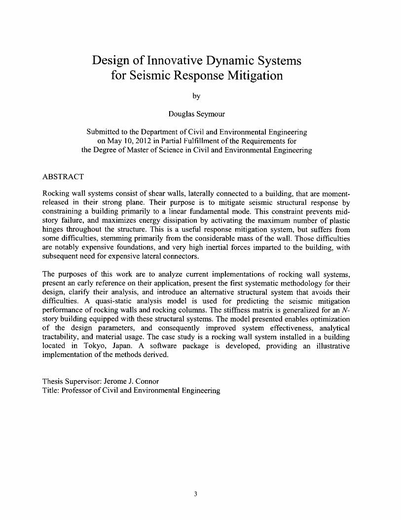
Submitted to the Department of Civil and Environmental Engineeringon May 10, 2012 in Partial Fulfillment of the Requirements for
the Degree of Master of Science in Civil and Environmental Engineering
ABSTRACT
Rocking wall systems consist of shear walls, laterally connected to a building, that are moment-released in their strong plane. Their purpose is to mitigate seismic structural response byconstraining a building primarily to a linear fundamental mode. This constraint prevents mid-story failure, and maximizes energy dissipation by activating the maximum number of plastichinges throughout the structure. This is a useful response mitigation system, but suffers fromsome difficulties, stemming primarily from the considerable mass of the wall. Those difficultiesare notably expensive foundations, and very high inertial forces imparted to the building, withsubsequent need for expensive lateral connectors.
The purposes of this work are to analyze current implementations of rocking wall systems,present an early reference on their application, present the first systematic methodology for theirdesign, clarify their analysis, and introduce an alternative structural system that avoids theirdifficulties. A quasi-static analysis model is used for predicting the seismic mitigationperformance of rocking walls and rocking columns. The stiffness matrix is generalized for an N-story building equipped with these structural systems. The model presented enables optimizationof the design parameters, and consequently improved system effectiveness, analyticaltractability, and material usage. The case study is a rocking wall system installed in a buildinglocated in Tokyo, Japan. A software package is developed, providing an illustrativeimplementation of the methods derived.
Thesis Supervisor: Jerome J. ConnorTitle: Professor of Civil and Environmental Engineering
3


Acknowledgments
I wish to give recognition to some of the many people who aided me in the completion of this
paper. First, to my advisor and friend Professor Jerry Connor, who taught me what it is to be a
civil engineer. Professor Connor suggested the topic, which is just one of a great many ideas that
he has helped me with. I would also like to thank my mechanical vibrations teacher and friend
Professor Eduardo Kausel for greatly advancing my understanding of vibrations.
I would also like to thank Professor Simon Laflamme, once Ph.D. candidate at MIT and now
professor at Iowa State University, for his help with the presentation of an earlier paper on this
topic, which aided my ability to produce a comprehensible academic paper tremendously. I
would also like to thank Professor Wada and Dr. Qu of the Tokyo Institute of Technology for
their assistance in providing data regarding the case study building. Professor Wada first sparked
my interest in rocking walls with a presentation he gave to Professor Connor's class in 2010, and
is presently the preeminent author in this field.
Douglas Seymour, April 2012
5


Contents
Page
1. Introduction 11
1.1. Rocking Walls within the Taxonomy of DynamicStructures
1.2. Outline and Purpose of Rocking Walls
1.3. Application of Rocking Walls 15
1.4. Outline History of Rocking Walls 16
2. Literature Review 18
2.1. Rocking Wall Design
2.1.1 Design for Resistance to Lateral Loads
2.1.2 Damping Design 19
2.1.3 Design for Serviceability
2.2. Lateral Load Bearing Capacity 20
2.3. Damping of Rocking Wall Systems 21
2.4. Ensuring Maximum Energy Dissipation with Linear 22Deformations
2.5. Case Study: Retrofit of the G3 Building 23
2.5.1. Response of the Case Study Building to Seismic Loading 26in the Transverse Direction
3. Rocking Wall Design 28
3.1. Problem Statement
3.2. Method
3.3. Introduction to Analytical Model 29
7

3.4. Solving an Analytical Model without Rocking Wall 31
3.5. Solving an Analytical Model with Rigid Rocking Wall
3.6. Solving an Analytical Model with Flexible Wall, 33Assumed Modes
3.7. Solving an Analytical Model with Flexible Wall, 34Assumed Modes, Full Analysis
3.8. Applying Seismic Action to the Analytical Model 38
3.9. Applying Static Equivalent Seismic Action 39
3.10. Solving an Analytical Model with Flexible Wall, 42with Full Stiffness Matrix
3.11 Benchmark Buildings 50
3.12. Software Implementation 52
3.13. Software to Implement ASCE 7-05 Equivalent Seismic 55Loads
4. Analysis of Rocking Wall Design 57
4.1. Natural Frequencies of the Simulations
4.2. Natural Frequencies of the System With and Without 58Rocking Wall
4.3. Modes of the System With Varying Stiffness ofRocking Wall
4.4. Maximum Story Drift Angle With Varying Rocking 60Wall Width
4.5. Forces Applied to the Building by the Rocking WallInertia 62
4.6. Comparison with Given Case Study Building Data 64
5. Study to Determine Whether the Case Study RockingWall Caused Damage During the Thhoku Earthquake 70
5.1. The Mathematical Model of the Building 71
5.2. Finite Element Modeling 72
5.3. Dynamics 75
8

5.4. Units and Consistency 77
5.5. Mass for Dynamic Analysis 78
5.6. Finding and Processing the Link Axial Forces in ADINA
5.7. The Addition of Damping to the Model 79
5.8. Calculation of the Static Shear Wall Cracking Moment 80
5.9. Conclusions of the Finite Element Study 81
6. Rocking Column Design 83
6.1. Rationale for Design
6.2. Introduction to Rocking Column Design 84
6.3. Further Rocking Column Design 86
6.4. Conclusions of the Finite Element Study 88
6.5. Conclusions of the Finite Element Study 89
6.6. Analysis of the Benefits of Rocking Columns 91
6.6.1 Lateral Force Reduction
6.6.2 Foundations Reduction 92
6.6.3 Cost Effective Connections
6.6.4 Greater Story Drift Reduction, with Potential for FurtherReductions
6.6.5 Overall Comparative Effectiveness 93
7. Suggested Extensions 94
8. Conclusions 95
9. References 97
9

10. Appendices 101
Appendix A. The 20 Significant United States Earthquakes 1933-2006 103
Appendix B. A Set of Benchmark Building Models for Use 125in Simulations
Appendix C. MATLAB Code for Solving the Rocking Wall as a 167Flexible Continuous System, using Lagrange
Appendix D. MATLAB Code to Find the Stiffness Matrix of 171Building-Rocking Wall System
10

1. Introduction
1.1. Rocking Walls within the Taxonomy of Dynamic Structures
Dynamic structures avoid structural damage by shifting the burden of energy dissipation to
chosen structural elements, preferably non-critical and replaceable elements. Damage that would
result in severe injury, and damage that would prevent future serviceability of the structure, can
be avoided by choosing the manner in which input energy is dissipated.
Dynamic Structures
F Linear AngularDisplacements Displacements
Base Isolation Rocking Walls
Figure 1.1.1. A partial taxonomy of dynamic structures
In addition to preventing loss of life, dynamic structures enable structures to be serviceable after
a seismic event, and as such can be a highly sustainable approach to structural design in
earthquake-prone regions.
1.2. Outline and Purpose of Rocking Walls
A rocking wall is a dynamic structural system that employs one or more stiff structural elements,
moment-released at the base, to force a building that is subjected to dynamic loads to fail in a
near-linear mode. This approach is intended to prevent mid-story failure, which is illustrated in
figure 1.4.1, by maximizing energy dissipation, as discussed in section 2.4. As illustrated in
11

figure 1.2.1, rocking walls are designed to rock only in the strong plane of the wall. This is in
strong contrast to a shear wall that is simply unrestrained at its base.
(a) (b) (C)
Figure 1.2.1. Schematic illustration of a simple unfixed shear wall contrasted with a rocking wall system.(a) Building with fixed shear wall, (b) Building with unfixed shear wall, (c) Building with rocking wall
All rocking walls have been constructed from reinforced concrete, as far as known at the time of
writing. As a result, the pin and foundations at the base of the wall must be highly substantial, as
illustrated in figure 2.1.2. Additionally, the lateral loads that the rocking wall imposes on the
surrounding structure during an earthquake are found, by an analytical method presented in this
work, to be very high partially due to the large mass of rocking wall, as discussed in section 4.5.
As a result, very substantial lateral supports are required to connect the rocking wall to the
building. All of these issues increase the cost of installation of a rocking wall system
substantially.
The Tokyo case study building, first introduced in section 2.5, was damaged in the
Tohoku earthquake of March 2011. Few buildings in Tokyo were significantly damaged in that
event, since as observed in Tokyo, the accelerations observed were one or two orders of
magnitude lower intensity than those observed nearer the epicenter. In section 5, a finite element
study is presented that supports the theory that the inertial loads from the rocking walls were
very high during the earthquake, and thus a rocking wall was in fact the cause of that damage.
12
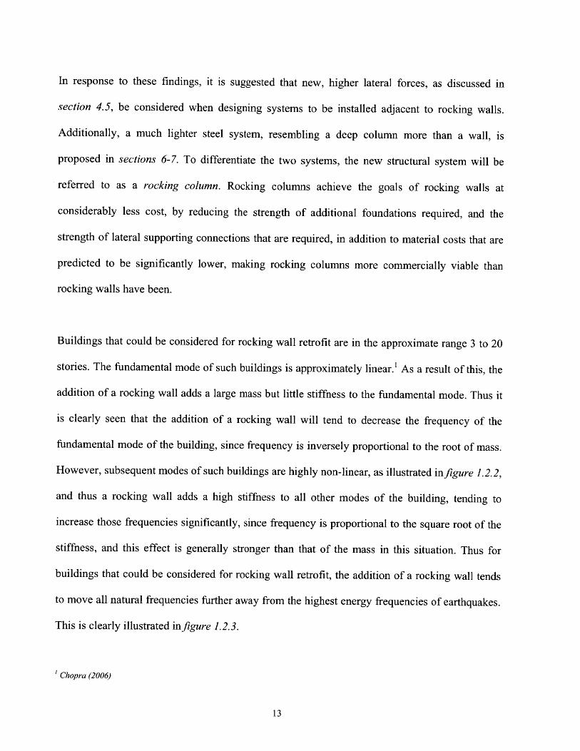
In response to these findings, it is suggested that new, higher lateral forces, as discussed in
section 4.5, be considered when designing systems to be installed adjacent to rocking walls.
Additionally, a much lighter steel system, resembling a deep column more than a wall, is
proposed in sections 6-7. To differentiate the two systems, the new structural system will be
referred to as a rocking column. Rocking columns achieve the goals of rocking walls at
considerably less cost, by reducing the strength of additional foundations required, and the
strength of lateral supporting connections that are required, in addition to material costs that are
predicted to be significantly lower, making rocking columns more commercially viable than
rocking walls have been.
Buildings that could be considered for rocking wall retrofit are in the approximate range 3 to 20
stories. The fundamental mode of such buildings is approximately linear.' As a result of this, the
addition of a rocking wall adds a large mass but little stiffness to the fundamental mode. Thus it
is clearly seen that the addition of a rocking wall will tend to decrease the frequency of the
fundamental mode of the building, since frequency is inversely proportional to the root of mass.
However, subsequent modes of such buildings are highly non-linear, as illustrated infigure 1.2.2,
and thus a rocking wall adds a high stiffness to all other modes of the building, tending to
increase those frequencies significantly, since frequency is proportional to the square root of the
stiffness, and this effect is generally stronger than that of the mass in this situation. Thus for
buildings that could be considered for rocking wall retrofit, the addition of a rocking wall tends
to move all natural frequencies further away from the highest energy frequencies of earthquakes.
This is clearly illustrated infigure 1.2.3.
' chopra (2006)
13
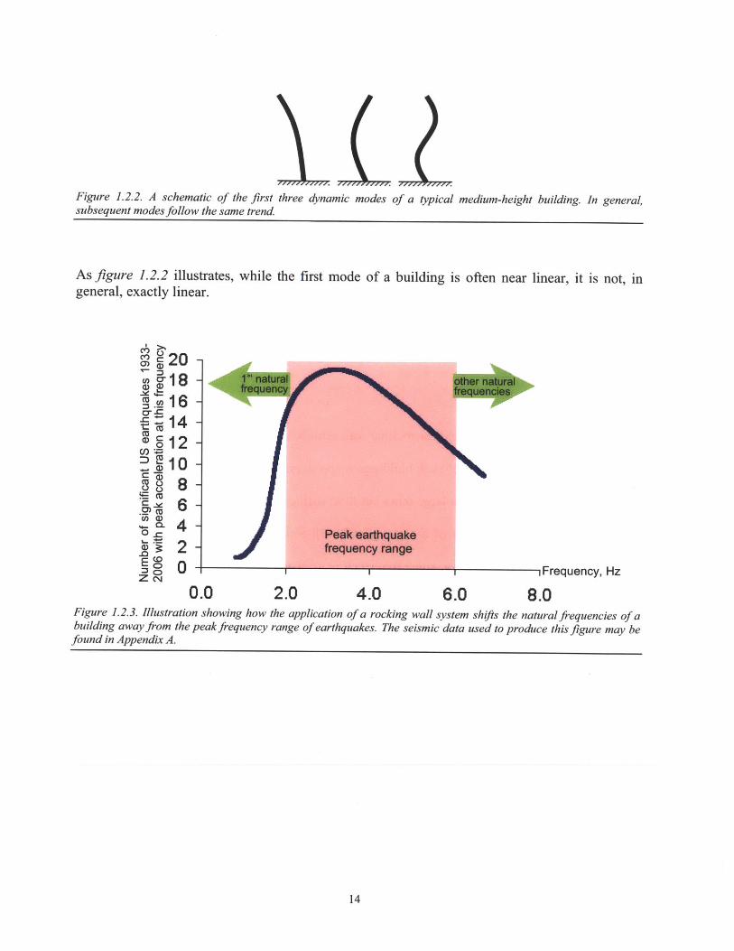
Figure 1.2.2. A schematic of the firstsubsequent modes follow the same trend
three dynamic modes of a typical medium-height building. In general,
As figure 1.2.2 illustrates,general, exactly linear.
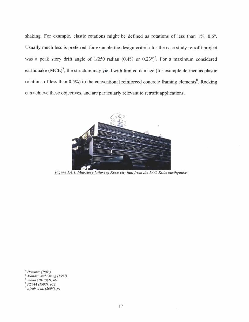
og20-
CI18 -. 16 -:14 -
6 --
o2 -
zo 00.0
while the first mode of a building is often near linear, it is not, in
Frequency, Hz
2.0 4.0 6.0 8.0Figure 1.2.3. Illustration showing how the application of a rocking wall system shifts the natural frequencies of abuilding away from the peak frequency range of earthquakes. The seismic data used to produce this figure may befound in Appendix A.
14

1.3. Application of Rocking Walls
For newly constructed buildings, there are many ways to prevent seismic damage, and a number
of ways to apply the benefits of dynamic structures. For example, the entire structural frame
could be allowed to rock, with energy dissipation being performed by replaceable fuses, as
illustrated infigure 1.3.1. However, clearly for existing structures such a solution is not feasible,
and other ways must be found to apply the benefits of dynamic structures.
Aroo~f
Post-Tensioning
Shear Fuse
Figure 1.3.1. A rocking frame structure.
Rocking wall retrofit projects are limited by the availability of appropriate locations to attach
rocking walls. Most often, such locations will be limited to the exterior of a building. In addition,
for buildings that are large in plan, rocking walls must be spaced at some reasonable distance
throughout the building. Clearly, it is not sufficient to use rocking walls to linearize the response
of a building in one location alone. Rocking walls must be spaced throughout the building to
ensure the whole response of the building is linearized under dynamic loading. This approach
can be seen in the case study introduced in section 2.5, a building which is large in plan, and uses
6 equally spaced rocking walls.
15

As will also be seen from that case study, the building to be retrofitted was long and thin, and the
rocking walls were to be installed to the exterior, as would be most common, as illustrated in
figure 2.5.2. This meant that it was only appropriate to install rocking walls in the longitudinal
direction of the building, since if rocking walls were installed to the transverse direction of the
building, the center of the building in plan would be largely unsupported, since the distance
between rocking walls would be very large. This would result in the desired linearized transverse
mode for the thin edges of the building in plan, but the transverse mode for the center of the
building in plan would remain unlinearized.
In general, there is no particular problem with installing rocking walls in both orientations of a
building. But in the case study, although rocking walls were added to the longitudinal direction,
it was decided to stiffen the transverse response by adding conventional transverse shear walls,
rather than add transverse rocking walls.
1.4. Outline History of Rocking Walls
The concept of rocking shear walls, though not in a form that matches current implementations,
was introduced by Ajrab et al.3 The work they presented was built on studies by Housner, who
investigated the free vibration of rigid rocking blocks.4
Mander and Cheng defined an approach to rocking, structural flexibility, and prestressing, as
damage avoidance design.5 The performance objective of the DAD philosophy for a maximum
assumed earthquake (MAE) is simply that the structure remains elastic at all times during ground
2 Deirlein (2010), p33 Ajrab et al. (2004)
16
shaking. For example, elastic rotations might be defined as rotations of less than 1%, 0.60.
Usually much less is preferred, for example the design criteria for the case study retrofit project
was a peak story drift angle of 1/250 radian (0.4% or 0.230)6. For a maximum considered
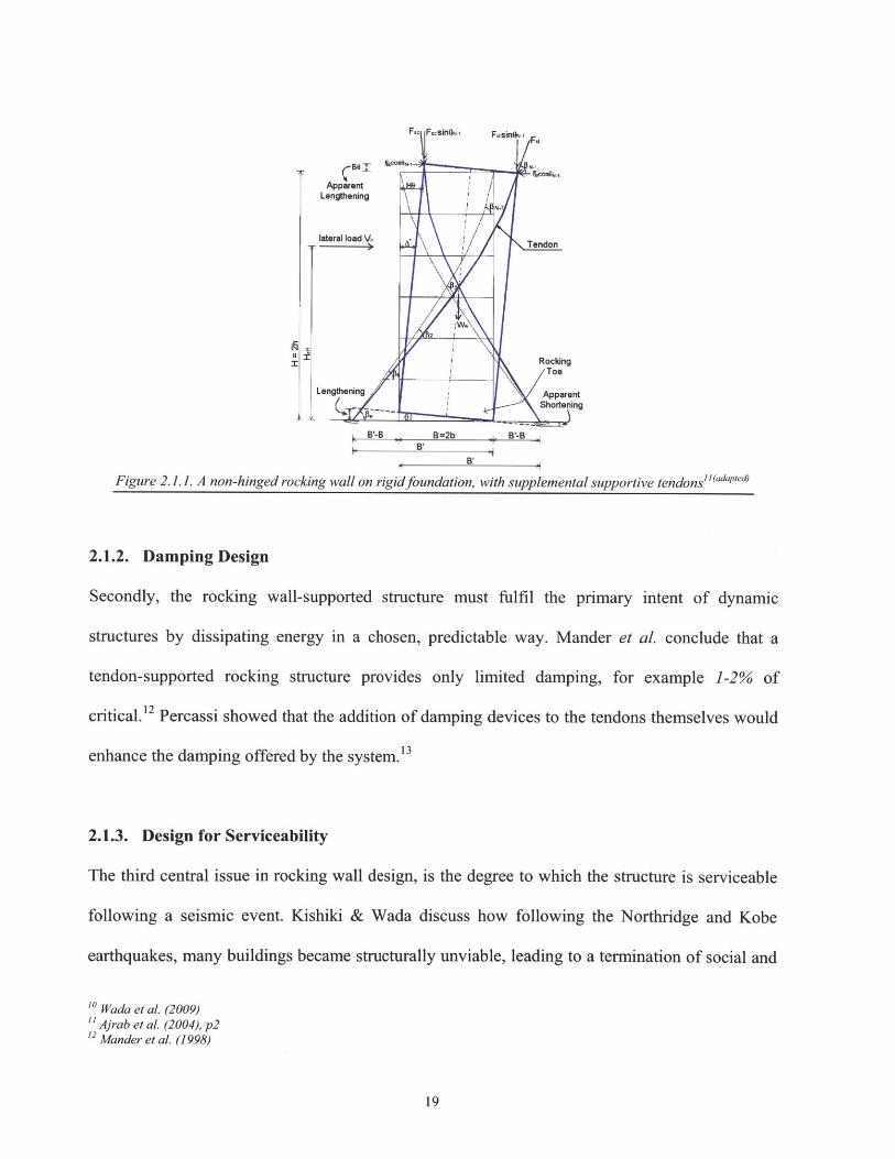
earthquake (MCE)7, the structure may yield with limited damage (for example defined as plastic
rotations of less than 0.5%) to the conventional reinforced concrete framing elements8 . Rocking
can achieve these objectives, and are particularly relevant to retrofit applications.
Figure 1.4.1. Mid-story failure of Kobe city hallfrom the 1995 Kobe earthquake.
' Housner (1963)5 Mander and Cheng (1997)6 Wada (2010)(2), p 6
7 FE MA (1997), p328 Ajrab et al. (2004), p 4
17

2. Literature Review
2.1. Rocking Wall Design
The present work proposes that rocking walls are most appropriate for retrofit applications, due
to their relatively high cost and less than ideal architectural characteristics. However, earlier
papers on this subject considered that rocking walls would be applied to new buildings, and play
a significant role in the primary lateral load bearing capacity of the structure.
2.1.1. Design for Resistance to Lateral Loads
There are three central issues that have been considered in rocking wall design. The first is that
adequate resistance to lateral loads must be maintained. Since it was originally proposed that the
moment capacity at the base of walls be removed, this load bearing capacity must be transferred
to three other classes of mechanism, being the moment capacity of shear wall-to-frame
connections, the resistance to overturning of the weight of the wall itself, and to additional
mechanisms, such as bracing, or post-tensioned tendons running through the wall, which are
illustrated infigure 2.1.1. Pekcan et al. suggested that such tendons be draped to match the shape
of the moment diagram induced under the assumed inertial loading.9 Note that the original
rocking wall concept presented is that of a flat base. If the rocking wall is pinned at the base, as
for example in the retrofit at the Tokyo Institute of Technology'0 , then clearly the weight of the
wall itself offers no moment resistance.
9 Pekcan et al. (2000)
18
.\
RockingToo
Lengthening ApparentShortening
B'-B B=2b B-BB'
B.
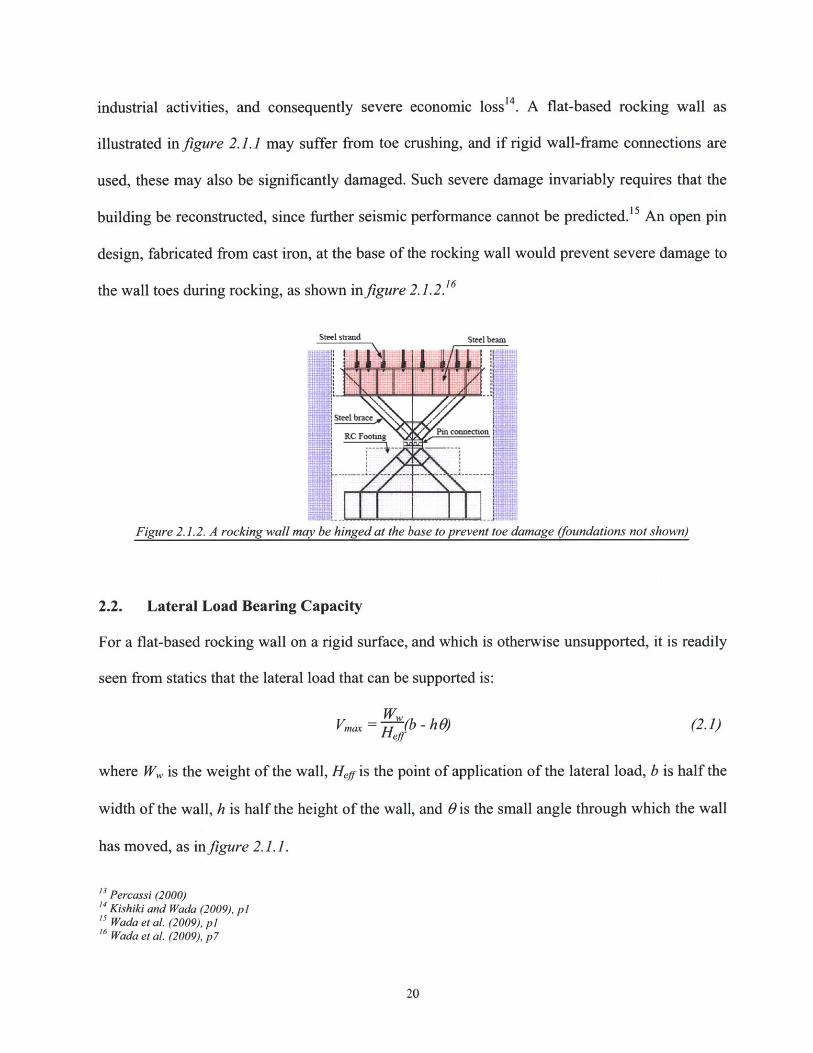
Figure 2.1.1. A non-hinged rocking wall on rigidfoundation, with supplemental supportive tendonsI(adaped)
2.1.2. Damping Design
Secondly, the rocking wall-supported structure must fulfil the primary intent of dynamic
structures by dissipating energy in a chosen, predictable way. Mander et al. conclude that a
tendon-supported rocking structure provides only limited damping, for example 1-2% of
critical. Percassi showed that the addition of damping devices to the tendons themselves would
enhance the damping offered by the system.' 3
2.1.3. Design for Serviceability
The third central issue in rocking wall design, is the degree to which the structure is serviceable
following a seismic event. Kishiki & Wada discuss how following the Northridge and Kobe
earthquakes, many buildings became structurally unviable, leading to a termination of social and
'0 Wada et al. (2009)1Ajrab et al. (2004), p2
12 Mander et al. (1998)
19
industrial activities, and consequently severe economic loss'4 . A flat-based rocking wall as
illustrated infigure 2.1.1 may suffer from toe crushing, and if rigid wall-frame connections are
used, these may also be significantly damaged. Such severe damage invariably requires that the
building be reconstructed, since further seismic performance cannot be predicted. 5 An open pin
design, fabricated from cast iron, at the base of the rocking wall would prevent severe damage to
the wall toes during rocking, as shown infigure 2.1.2.16
Steel strand Steel beam
3RC Footmg Pmcneto
Figure 2.1.2. A rocking wall may be hinged at the base to prevent toe damage (foundations not shown)
2.2. Lateral Load Bearing Capacity
For a flat-based rocking wall on a rigid surface, and which is otherwise unsupported, it is readily
seen from statics that the lateral load that can be supported is:
WVax = (b - h) (2.1)Heff(21
where W, is the weight of the wall, Heff is the point of application of the lateral load, b is half the
width of the wall, h is half the height of the wall, and 0 is the small angle through which the wall
has moved, as in figure 2.1.1.
13 Percassi (2000)" Kishiki and Wada (2009), p1
' Wada et aL. (2009), p1
1 Wada et aL. (2009), p 7
20
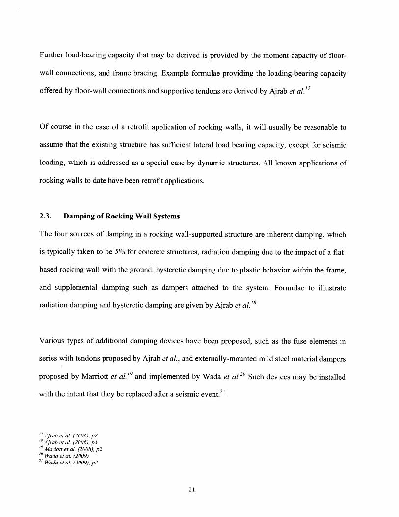
Further load-bearing capacity that may be derived is provided by the moment capacity of floor-
wall connections, and frame bracing. Example formulae providing the loading-bearing capacity
offered by floor-wall connections and supportive tendons are derived by Ajrab et al."
Of course in the case of a retrofit application of rocking walls, it will usually be reasonable to
assume that the existing structure has sufficient lateral load bearing capacity, except for seismic
loading, which is addressed as a special case by dynamic structures. All known applications of
rocking walls to date have been retrofit applications.
2.3. Damping of Rocking Wall Systems
The four sources of damping in a rocking wall-supported structure are inherent damping, which
is typically taken to be 5% for concrete structures, radiation damping due to the impact of a flat-
based rocking wall with the ground, hysteretic damping due to plastic behavior within the frame,
and supplemental damping such as dampers attached to the system. Formulae to illustrate
radiation damping and hysteretic damping are given by Ajrab et al.18
Various types of additional damping devices have been proposed, such as the fuse elements in
series with tendons proposed by Ajrab et al., and externally-mounted mild steel material dampers
proposed by Marriott et al.19 and implemented by Wada et al.2 0 Such devices may be installed
with the intent that they be replaced after a seismic event.2 1
7 Ajrab et al. (2006), p21 Ajrab et al. (2006), p31 Mariott et al. (2008), p220 Wada et al. (2009)2] Wada et al. (2009), p2
21

2.4. Ensuring Maximum Energy Dissipation with Linear Deformations
The introduction of rocking wall system to a frame building may be motivated by showing the
benefit of a global failure mode with low rotations as opposed to a local failure mode with high
rotations. Consider for example the simple frame with the three failure modes shown in figure
2.4.1.
Figure 2.4.1. (a) A schematic 3 story frame, (b), (c) its two non-ideal pushover failure modes, (d) its ideal pushoverfailure mode
It is readily seen that as the number of plastic hinges increases in the failure mode, so does the
ability of the structure to dissipate energy. The first two failure modes shown have low energy
dissipation, and so the rotations induced will be large, with high potential for loss of life and
severe structural damage. However the final failure mode uses all possible plastic hinges, and
thus has the maximum energy dissipation per unit rotation. Thus in this mode the rotations will
be smaller, and the probability of saving life and further structural serviceability is maximized.
22 Wada et al. (2009), p2
22
Hence the focus for seismic retrofit need not be strengthening the individual members which
would deform excessively under seismic loading, but rather the control of the global behaviour
of the structure to prevent damage from weak modes.
Additionally, it may be noted that the non-ideal failure modes are more likely to occur under
higher-mode excitation, since those forms are more congruent with the higher mode shapes, as
illustrated infigure 1.2.2.
Hence, if a rocking wall is designed to be rigid enough to resist the partial failure modes, the
frame will tend to fail in the preferable global failure mode. A rocking wall thus suppresses
higher mode vibrations,2 4 by moving the natural frequencies away from the peak energy range of
earthquakes, as seen infigure 1.2.3.
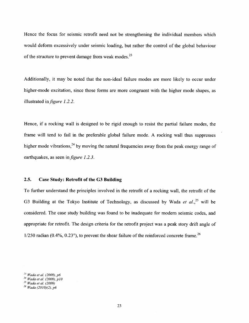
2.5. Case Study: Retrofit of the G3 Building
To further understand the principles involved in the retrofit of a rocking wall, the retrofit of the
G3 Building at the Tokyo Institute of Technology, as discussed by Wada et al.,5 will be
considered. The case study building was found to be inadequate for modem seismic codes, and
appropriate for retrofit. The design criteria for the retrofit project was a peak story drift angle of
1/250 radian (0.4%, 0.230), to prevent the shear failure of the reinforced concrete frame. 26
23 Wada et al. (2009), p624 Wada et al. (2009), pl021 Wada et al. (2009)26 Wada (2010)(2), p6
23

Figure 2.5.1. (a) The case study building in the Suzukakedai Campus of the Tokyo Institute of Technologyz,(aapted),(b) A 3D model of the retrofitted case study building, where yellow represents new structure to be retrofitted".
As is seen from figures 2.5.1(b) and 2.5.2, the design proposed by Wada et al. consists of wide
and shallow rocking walls (14.4ft by 2ft in plan) which rock in the longitudinal direction of the
building. The rocking walls represent an additional 56% of the existing steel reinforced concrete
frame area, in plan. The wall is prestressed to allow for the large vertical tensile forces which
will result from inertial motion, and is designed to remain elastic during severe seismic motion.29
As is seen fromfigure 2.5.2, this retrofit only stiffens the response at six approximately evenly-
distributed locations. The existing floor diaphragm stiffness between the rocking walls is
21 Wada (2010)(2)
24
I G3 [
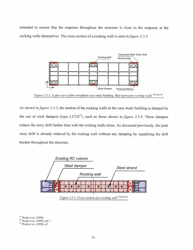
intended to ensure that the response throughout the structure is close to the response at the
rocking walls themselves. The cross section-of a rocking wall is seen infigure 2.5.3.
Transverse Static Shear WallRocking Wall Rocking Wall
x Steel Damper Horizontal Brace
Figure 2.5.2. A plan view of the retrofitted case study building. Red represents rocking walls.30(adapied)
As shown infigure 2.5.3, the motion of the rocking walls in the case study building is damped by
the use of steel dampers (type LY22631), such as those shown in figure 2.5.4. These dampers
reduce the story drift further than with the rocking walls alone. As discussed previously, the peak
story drift is already reduced by the rocking wall without any damping by equalizing the drift
burden throughout the structure.
Existing RC column
Steel damper
Rocking wall
Steel strand
-f P. .1 T, 7 374 T, i;1 M I
4
H
a t 0 1
Figure 2.5.3. Cross-section of a rocking Wall. 32,adapledl
28 Wada et aL. (2009)21 Wada et al. (2009), p6-7so Wada et al. (2009), p5
25
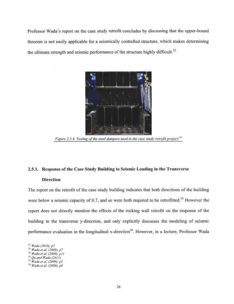
Professor Wada's report on the case study retrofit concludes by discussing that the upper-bound
theorem is not easily applicable for a seismically controlled structure, which makes determining
the ultimate strength and seismic performance of the structure highly difficult.3 3
Figure 2.5.4. Testing of the steel dampers used in the case study retrofit project. 3 4
2.5.1. Response of the Case Study Building to Seismic Loading in the Transverse
Direction
The report on the retrofit of the case study building indicates that both directions of the building
were below a seismic capacity of 0.7, and so were both required to be retrofitted. However the
report does not directly mention the effects of the rocking wall retrofit on the response of the
building in the transverse y-direction, and only explicitly discusses the modeling of seismic
performance evaluation in the longitudinal x-direction 36. However, in a lecture, Professor Wada
3' Wada (2010), p732 Wada et al. (2009), p 7
3 Wada et al. (2009), p 1134 Qu and Wada (2011)3s Wada et al. (2009), p536 Wada et al. (2009), p8
26

mentioned the additional static shear walls which were added to the transverse direction3 7, and
which are seen infigure 2.5.1. When a student asked about this issue, Professor Wada remarked
that the retrofitted building is adequately stiff in the transverse direction to resist severe damage,
and that the project is designed for 225% of the code requirements. 38
3 Wada (2010)(2), p738 Wada (2010)(1)
27

3. Rocking Wall Design
3.1. Problem Statement
Currently, each rocking wall design project requires an entirely new analysis from first
principles, with expert-level oversight. Such high design requirements are prohibitive in the
application of any new system. To aid in future maturation and acceptance of this structural
system, it is required to provide tools that systematize the selection of rocking wall properties,
based on the known parameters of the building to be retrofitted, to reduce the time required for
the analysis phase, and provide a framework for design. This will allow engineers to better
understand the structural system and aid discussion in this area of dynamic structures.
The most critical information to determine is the size of rocking wall that is required for a given
building. Secondly, it is required to determine the lateral loads that the rocking wall applies to
the building under code-determined seismic loading.
3.2. Method
In this work, the process of producing the tools alluded to in the problem statement is started
with the development of a number of analytical models of the rocking wall system, in sections
3.3 - 3.7 and 3.10.
A method is developed which may generate benchmark discretized buildings of any number of
stories, including story stiffnesses and story masses, such that the analytical model of the
discretized building-rocking wall system may be applied to them, as discussed in section 3.11.
28

Seismic loads are applied to the analytical model, and the responses of the model to those loads
are analyzed, as discussed in sections 3.8 - 3.9.
Example software is developed which implements those models programmatically, and returns
the required information, as discussed in sections 3.12 - 3.13.
3.3. Introduction to Analytical Model
For low- to medium-rise structures, which are the primary focus of retrofitting rocking walls,
buildings tend to deform approximately like a shear beam, under environmental loads. If the
building deformation were exactly linear, as shown in figure 3.3.1, then clearly a rocking wall
would add no stiffness to that particular deformation, only mass. In general this is close to the
truth for fundamental mode deformations. Although for all buildings with stiffness profiles that
are not parabolic, there will be some non-linearity in the deformation under seismic loading.39
Figure 3.3.1. Low- to medium-rise buildings tend to deform like a shear beam
The principle of tributary areas can be used to model a low-rise building with an attached
rocking wall as shown infigure 3.3.2.
3 Connor (2003)
29

M2 u,,M2 -+- U2
k2 h k, hMJ {MJ j,--O-U , Uk1 h ki h
Figure 3.3.2. Schematic of a tributary two-story building model with rocking wall (a) without supplementaldamping, (b) with supplemental damping
Initially, the rocking wall will be modeled as rigid. In subsequent models, the wall will be
modeled as having finite rigidity, with the intent that an optimum rigidity will be found that
maintains purely elastic deformation in the structure.
Initially, Lagrange's equation will be solved without taking the ground motion into account.
Assuming deflections are small, a condition which the rocking wall is intended to enforce,
changes in gravitational potential energy may be neglected, and the stiffness of the columns may
be assumed to remain linear.
Three models of the rocking wall-building system are presented, of increasing complexity. First
a model with a rigid wall is presented, then a model with a flexible wall, and finally the complete
analytical stiffness matrix of the system will be presented.
30
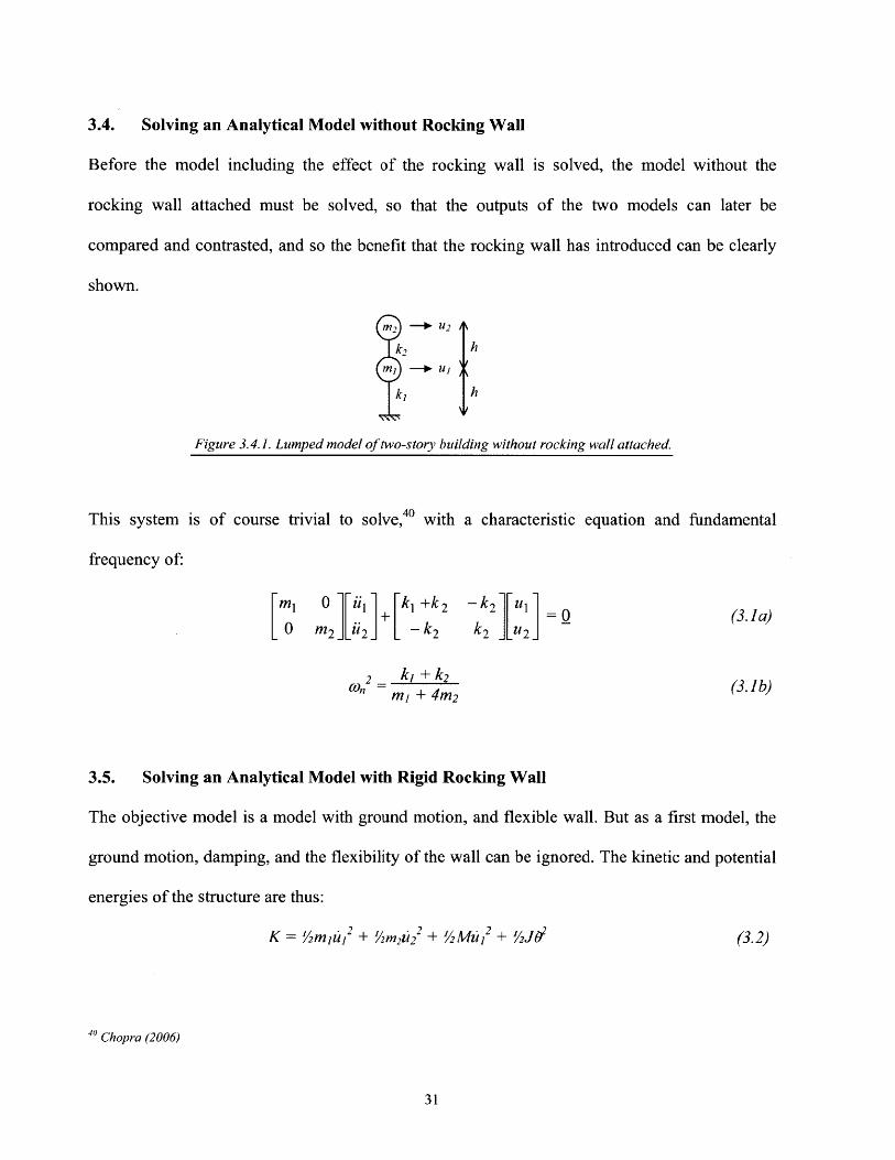
3.4. Solving an Analytical Model without Rocking Wall
Before the model including the effect of the rocking wall is solved, the model without the
rocking wall attached must be solved, so that the outputs of the two models can later be
compared and contrasted, and so the benefit that the rocking wall has introduced can be clearly
shown.
k, h
ki h
Figure 3.4.1. Lumped model of two-story building without rocking wall attached.
This system is of course trivial to solve,40 with a characteristic equation and fundamental
frequency of:
[ 1 O1 +[kl ±k 2 -k 2 =U 0 (3.1a)[0 m 2 ji_ 2 [ - k2 k2 ju 2 j
Col2= kI +k2 (.1b=mi (3.b)
3.5. Solving an Analytical Model with Rigid Rocking Wall
The objective model is a model with ground motion, and flexible wall. But as a first model, the
ground motion, damping, and the flexibility of the wall can be ignored. The kinetic and potential
energies of the structure are thus:
K = %Amiu| + %1m2 U2 + Y2MZI+ %J (3.2)
'0 Chopra (2006)
31

V = %k2u 2 + ki(u2 - 2 (3.3)
However, since the rocking wall is initially being modeled as rigid, and small rotations are
assumed, the geometric conditions exist:
u2= 2ui
=
and so without damping:
(3.4)
(3.5)
K = %Am 1u + 2m2d| + %2Mb 2 + %2 h S%(mi + 4M2 + M + )u)
V = %k 2 u, + % kul =(k, + k2)u
= (mi + 4m2 + M+
-l l 0
-(ki + k2)ui
Jv2hI,)|
J
(3.6)
(3.7)
(3.8)
(3.9)
(3.10)
Thus from Lagrange's equation, the unforced equation of motion and natural frequency of the
structure are shown to be:
J(mi + 4m2 + M+ )iI + (k, + k 2)ui = 0 (3.11)
(3.12)m, +4m2 + M + 2h
Thus, assuming an approximately linear mode both with and without the rocking wall, the
rocking wall decreases the fundamental frequency by an amount equal to 1M+
m, + 4M2
32

3.6 Solving an Analytical Model with Flexible Wall, Assumed Modes
This model is somewhat more realistic, but significantly more complex. In addition to a rigid
mode, an appropriate non-rigid mode shall be superposed. It is noted that the first non-rigid
mode and frequency of an ideal pin-ended beam free at the other end are:41
OD1 = (N) (3.17)Q AL2
1sinh cxx ZRt1 = sin c - asinh (L ere a= 4L
which, asfigure 3.6.1 shows, may be approximated as:
VI ~~-sin x
(3.18)
(3.19)
C1 sin CD
Figure 3.6. 1. The non-rigid trial mode (a) y,=sin ox - Isinh ox (b) Vi sin atc
Clearly, the rigid body mode is:
xYO =T
Thus, if the following deformation form is assumed:
u = yloqo(t) + yiuqi(t)
(3.20)
(3.21)
' Kausel (2010)
33
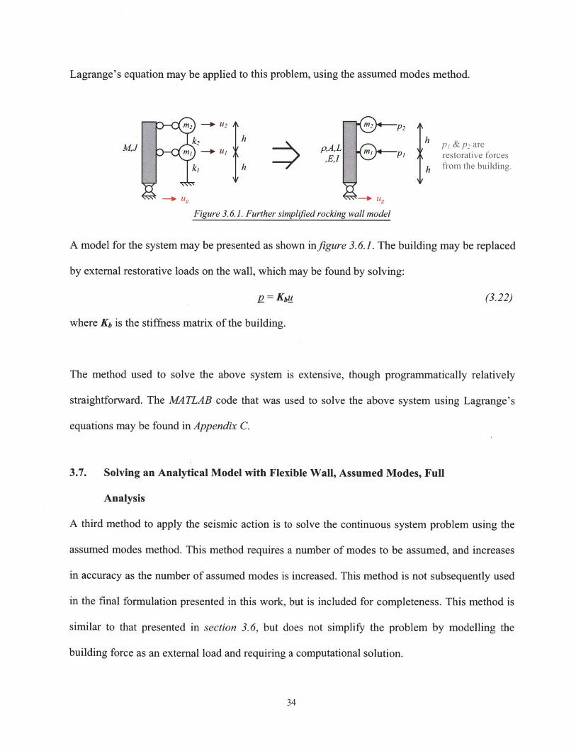
Lagrange's equation may be applied to this problem, using the assumed modes method.
M2 -+- u' ,,mUp2,
kh h hM, J m-u;'pA,L mI PI & P2. are
M, EI0 Pi ,, restorative forces
k h h from the building.
-+ ug ug
Figure 3.6.1. Further simplified rocking wall model
A model for the system may be presented as shown infigure 3.6.1. The building may be replaced
by external restorative loads on the wall, which may be found by solving:
p=Kiu (3.22)
where Kb is the stiffness matrix of the building.
The method used to solve the above system is extensive, though programmatically relatively
straightforward. The MA TLAB code that was used to solve the above system using Lagrange's
equations may be found in Appendix C.
3.7. Solving an Analytical Model with Flexible Wall, Assumed Modes, Full
Analysis
A third method to apply the seismic action is to solve the continuous system problem using the
assumed modes method. This method requires a number of modes to be assumed, and increases
in accuracy as the number of assumed modes is increased. This method is not subsequently used
in the final formulation presented in this work, but is included for completeness. This method is
similar to that presented in section 3.6, but does not simplify the problem by modelling the
building force as an external load and requiring a computational solution.
34

In this formulation, two modes are considered: a linear mode /o, and a chosen mode y, for
which a good choice would be either of the modes shown in figure 3.6.1. In the following
derivation, u represents the absolute displacement and v the relative displacement to the ground.
Consider the general problem as shown infigure 3.7.1:
Akx
k
xa =aLmu x:t
k X= cpL
Ug (t)
Figure 3.7.1. The rocking wall problem generalized
Fromfigure 3.7.1, it is observed that:
u(x,t)=v(x,t )+ug , i, ( =u(x,,,t)= u(aL,t), (3.23)
u, (t) = u(x,,t ) =u(8L,t) (3.24)
Now define:
K (aL) yj, , ,8L )= V1,,, (3.25)
then:
K k -ILl2 pAdx + _m'1d +_jm Zd2 2JuP1wTma 2m16 13
{ (Q+d,) 2 pAdx+m, (9,, + dg) + m,(9, +d, )2 (3.26)
L=j(4 +y,4,+tdg) pAdx+m,(a4)0 +yIa.4,+ig):+m,{(I340+y,14 ,i+d
35
=pA (L 4 +± , ++ , &)dx+m aaa4 + .4,+dg]mI 8[840 + Y,4, +d,
=PA x2 dx + IIxdx+ fxdx +a2m+2m,) 4o (3.27)
+(ama + pm,y 1 0 ) 4 +(maa + mp)ii
= pA (4 + 4 + )V,+dx +may/,,(a 40 + yi+d,m + ,, + i,
=pA x 1 dx+ j dx+dL I Idx] + (aV,,ma + PIm)4 0 (3.28)
+/2 Ma + iy1m, )4, +(VIama + yIflmf dg
Hence differentiate these to find:
d BK ( pAL+a2ma +/2mp)ijodt 84 0
3 (3.29)
+ jpA yxdx+a may,,a + /my 1, ij, + ({ pAL + maa + m,,p)fig
[±pA xy 1 dx+ayIma +fym, (
+[pA. dx+y2ma +V 2 mf 4 + pA, dx+yima+ym fig
Also:
V ={ Ev"2 d+k. (va -v_ +jk,v,v2+ EI (vf) dx + ( -)2 ++ (3.31)
= j EIj(y"q1)2 dx+{ ka ((a -,0)qO +(yfa -y2ifl)qI) +jk,8 pq0 +yI,6qI)
=k a a- 8)(a - )q O+ ( - Y ,)q l+ k ,6,8 qo + ,( .2q,)aqO (3.32)
=[(a - 0)2k k,2k, IqO +(a -18)(Via - V ,0 )k, + pY1Igk, q,
36

av q
(3.33)= [(a - V/)(yi , - y/i, )ka + PytIk, Iq 0 + [EI N(yidx+(VIa - Y, ) 2 k, + Y2 k q,
Finally, applying Lagrange's equations:
M + Kq = -muig
where:
= pAL +a2 ma +/J2 m
{±pA fx y1, dx +a Iama + 6VI,,,m,
IpA Vy,xdx+amaylia
pA y / dx + y/ m, + Y/2 M
+I#myiyf
J (3.34)
(3.35)(a -p) 2 k" +,8 2k,
K-=
(a -p8)(y/l -YI11)ka +py/,,pk,
Sp AL+maa+mpM= , q= {qO (3.36)
pA yK, dx + y!,my/lfm, qJ
Thus using the above formulation, the ground acceleration "g may be set to be the maximum
ground acceleration Sa for a certain considered earthquake, and the system solved for that case.
37
(a - p)r- yV 13) ka +8 Vy!,6k,
E L(/,) dx + (y -gI)2 k, + r,k6

3.8. Applying Seismic Action to the Analytical Model
Applying seismic action to a model can be achieved a number of ways. To solve discrete
systems, the mass and stiffness matrices of the whole system M & K may be found, and the
system solved for an earthquake ground acceleration flg:42
MV+ Cv + Kv = -Meig (3.37)
where e is the unit constant rigid body vector, and v is the relative displacement:
v = u- eug (3.38)
However, in order to model the rocking wall, a continuous element, another approach must be
taken. One option is to discretize the rocking wall into lumped masses, and solve the problem as
a discrete dynamic system. The other is to solve the flexible wall problem fully analytically as in
section 3.7.
The quasi-static approach to applying seismic action is to apply forces, which are proportional to
the square of the height, to the masses of the building. The values of these forces may be found
analytically, and guides to aid their calculation are found in building codes. To solve the rocking
wall as a statics problem, these loads may be applied to the analytical model, and find the
resultant displacements.
To achieve either of the above methods of applying the seismic action, the stiffness matrix for
the rocking wall-building system must be determined. This may be found empirically, for
example using a finite element approach for a specific system under consideration.43 However, it
42 Chopra (2006)4 Bathe (1996)
38
would be far more valuable to determine the general analytical stiffness matrix of this system, for
any given system parameters. That stiffness matrix is derived in Section 3.10.
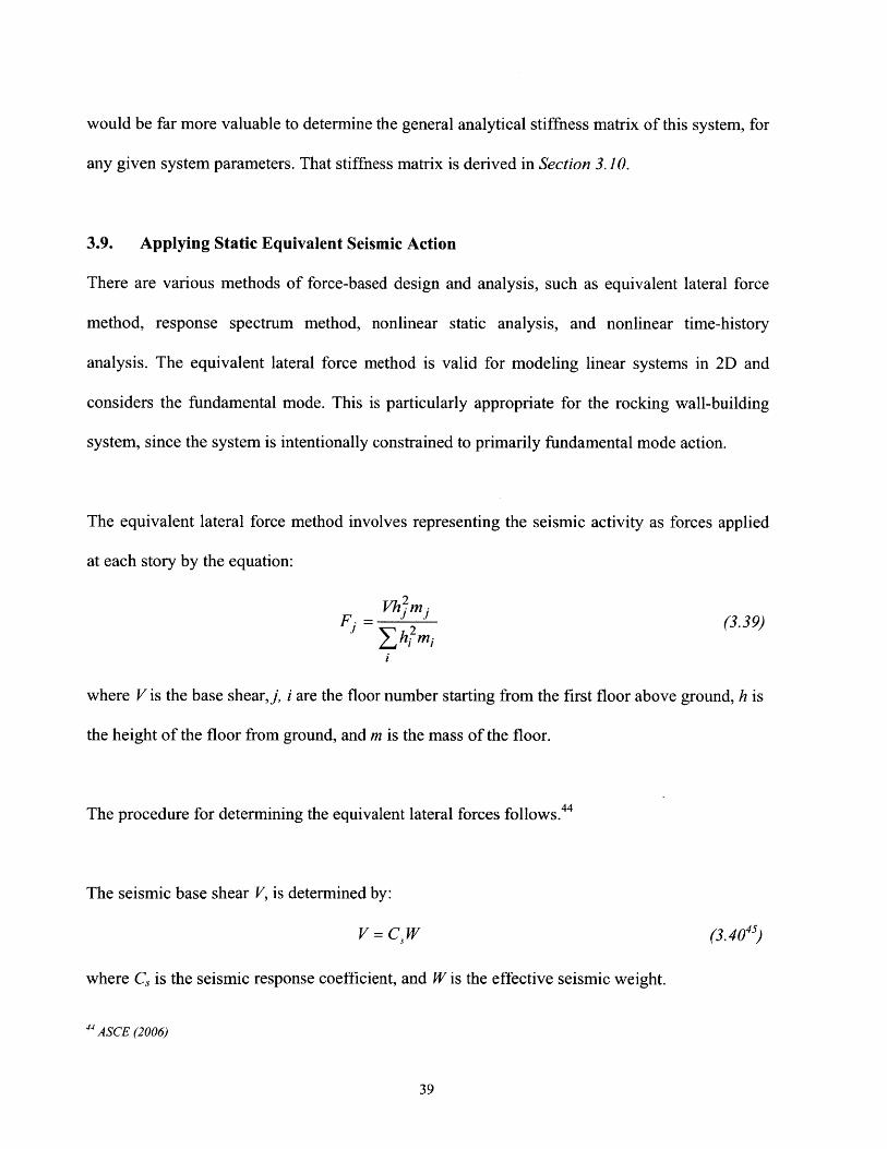
3.9. Applying Static Equivalent Seismic Action
There are various methods of force-based design and analysis, such as equivalent lateral force
method, response spectrum method, nonlinear static analysis, and nonlinear time-history
analysis. The equivalent lateral force method is valid for modeling linear systems in 2D and
considers the fundamental mode. This is particularly appropriate for the rocking wall-building
system, since the system is intentionally constrained to primarily fundamental mode action.
The equivalent lateral force method involves representing the seismic activity as forces applied
at each story by the equation:
Vh 2
Fj - = (3.39)Y hi2mi
where V is the base shearj, i are the floor number starting from the first floor above ground, h is
the height of the floor from ground, and m is the mass of the floor.
The procedure for determining the equivalent lateral forces follows. 4 4
The seismic base shear V, is determined by:
V = CW (3.4045)
where C, is the seismic response coefficient, and W is the effective seismic weight.
44 ASCE (2006)
39

The effective seismic weight of the building W, is defined by the code. 46 Cs is given by:
SWCS = SDS
(R)
47
where SDs is the design spectral response acceleration at short period, R is the response
modification factor, and I is the occupancy importance factor.
The design earthquake spectral response acceleration parameter at short period, SDS, is given by:
SDS MS3(3.42 48)
where SMs, the Maximum Considered Earthquake (MCE) spectral response acceleration for short
periods, is given by:
SMS = F.S, (3.4349)
Here, S, is the mapped MCE spectral response acceleration at short periods and Fa is a site
coefficient. Fa is dependent on the Site Class and Ss. Ss is determined from the 0.2s spectral
response accelerations as shown by a contour map of the Unites States given in a specified
figure.
The code states that "Where the soil properties are not known in sufficient detail to determine the
site class, Site Class D shall be used.".5 In that case, Fa is found to be 1.6.
4sASCE (2006), Eqn. 12.8-14 6 ASCE (2006), Section 12.7.247ASCE (2006), Eqn. 12.8-248ASCE (2006), Eqn. 11.4-3* ASCE (2006), Eqn. 11.4-15 0 ASCE (2006), Figure 22-1si ASCE (2006), Section 20.1
40

Assuming an Occupancy Category of j,53 the importance factor, I, is determined to be 1.25.
The response modification factor R is determined to be 4, assuming an ordinary reinforced
concrete shear wall.
The value of Cs must not exceed:
C, = SD1
TR)
T
C, = SDTL
T 2(RI)
for T !TL (3.4 5)
for T >TL (3. 46'7)
Additionally, Cs must not be less than 0.01.58
For structures located where S, > 0.6g, C, must not be less than:
0.5SC=C IJ (3.4 759)
(R)
In the above formulae, SDI, TL, T, and Si are to be evaluated.
SDI is the design earthquake spectral response acceleration parameter at Is period, and it is
determined by:
52 ASCE (2006), Table 11.4-1
5 3 ASCE (2006), Table 1-I54ASCE (2006), Table 11.5-1"5 ASCE (2006), Table 12.2-15 6 ASCE (2006), Eqn. 12.8-357ASCE (2006), Eqn. 12.8-458ASCE (2006), Eqn. 12.8-5* ASCE (2006), Eqn. 12.8-6
41

SDI = 2S3
SMI, the MCE spectral response acceleration at Is period, is determined by:
S, = F SI
(3.4860)
(3.4961)
Si, the mapped MCE spectral response acceleration at a period of Is, is determined from a
specified figure, 62 and F,, a site coefficient, is determined from a specified table.63
T is the fundamental period of the structure. The approximate period Ta
T, = C,h'n
where h, is the height in feet above the base to the highest level
coefficients C, and x are determined from a specified table.65
is found by the formula:
(3.5064)
of the structure and the
3.10. Solving an Analytical Model with Flexible Wall, with Full Stiffness Matrix
The full analytical model of the rocking wall-discretized building system, concluding with the
definition of the general stiffness matrix for this system, is first derived in this section.
60 ASCE (2006), Eqn. 11.4-4
" ASCE (2006), Eqn. 11.4-262 ASCE (2006), Figure 22-263 ASCE (2006), Table 11.4-21 ASCE (2006), Eqn. 12.8-7
42

Figure 3.10.1. The statically condensed rocking wall-building system to be modeled.
The rocking wall-structure system is illustrated in figure 3.10.1, in which k, and m; represent the
stiffness and tributary mass respectively of the ith story. The development of the model begins by
representing the rocking wall as a hinged beam, as shown infigure 3.10.2, in which F; represent
any loading on the beam that is constrained to static equilibrium.
L
F1 F 2 FN
Figure 3.10.2. Model of the free rocking wall.
Computing moments about the pin, assuming constant inter-story height for simplicity, and
setting the lowermost force to be a function of the others, an expression to describe the link
forces Fi is obtained,
Fi = -2F 2 - 3F3 ...- NFN (3.51)
6 5ASCE (2006), Table 12.8-2
43
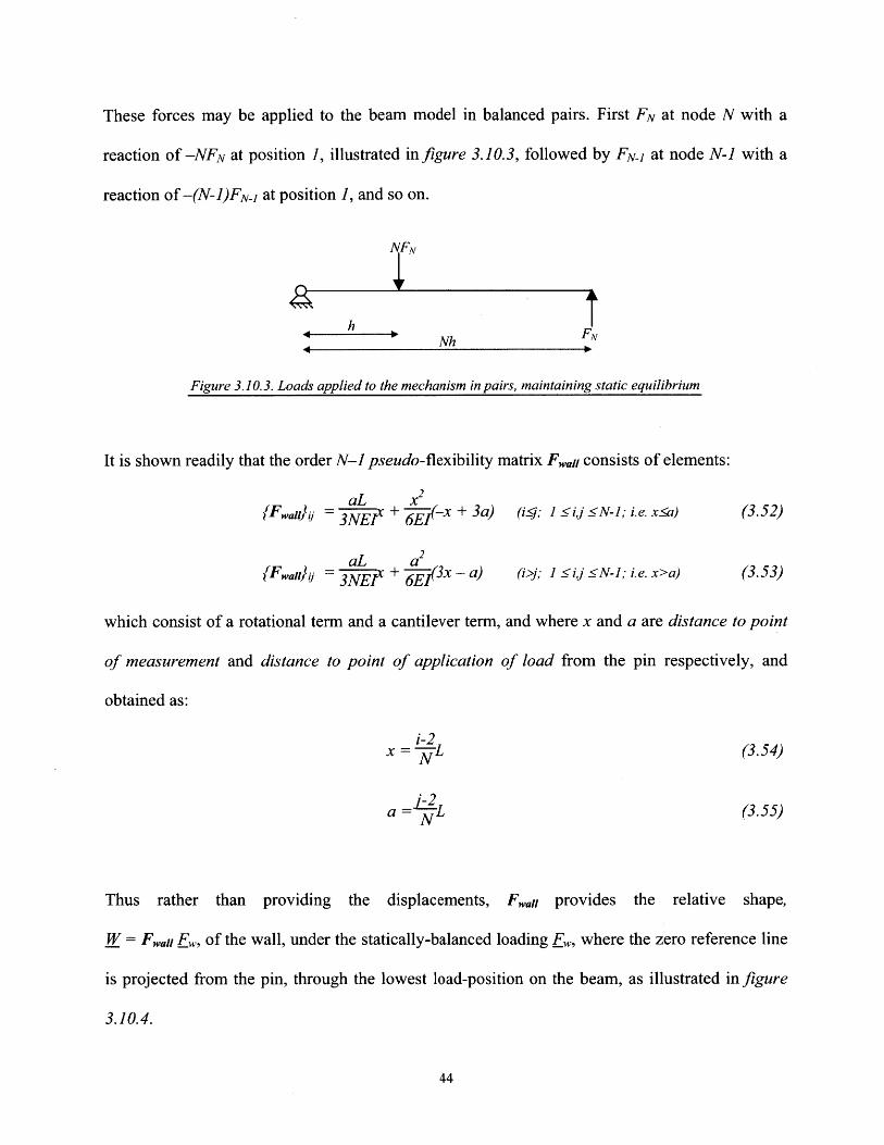
These forces may be applied to the beam model in balanced pairs. First FN at node N with a
reaction of -NFN at position 1, illustrated in figure 3.10.3, followed by FN-1 at node N-1 with a
reaction of -(N-1)FN-1 at position 1, and so on.
NFN
h Ah FN
Figure 3.10.3. Loads applied to the mechanism in pairs, maintaining static equilibrium
It is shown readily that the order N-1 pseudo-flexibility matrix Ewaji consists of elements:
{Fwai = 3-x + 3a) (ij; 1 i,j N-1; i.e. xsa) (3.52)l~al)i=3NEf ± + 3a
aL a2{Fwaiiaii = 3NEf ± (3X - a) (i>j; I :sij!N-1; i.e. x>a) (3.53)
which consist of a rotational term and a cantilever term, and where x and a are distance to point
of measurement and distance to point of application of load from the pin respectively, and
obtained as:
i-2
x = NL (3.54)
a = L (3.55)
Thus rather than providing the displacements, Fwall provides the relative shape,
W = F 11 F, of the wall, under the statically-balanced loading F, where the zero reference line
is projected from the pin, through the lowest load-position on the beam, as illustrated in figure
3.10.4.
44

N
(W
(II
Figure 3.10.4. The model beam under an arbitrary loading and dejormation. The reference line, shown dashed,coincides with the lowest beam reference position, requiring that the relative displacement W1=0. yV is the smallangle through which the reference line is displaced.
A vector of displacements relative to the reference line may be defined as W. The total
displacement of the wall is given by _E, plus a rigid body rotation. For now, let W be of size N-1,
omitting the lowest relative displacement W = 0. The analysis may be continued by recognizing
that since the beam is a mechanism, it may be rotated to any arbitrary small angle V under an
arbitrary balanced loading, such that the absolute positions of the beam are a rigid body rotation
displacement j, plus the deviations from that line, _W. Additional information is required to fix
the beam in space. Consider the model in figure 3.10.5, where U, V, P, Q, and F are vectors of
displacements of the building and wall, loading on the building and wall, and link forces
respectively.
45

UN, QN -)
U, Q; -M -- V, P,F, F,
Figure 3.10.5. The rocking wall-building system model with forces and displacements required to complete theanalysis
From the previous discussion, a matrix Fwalu that uniquely maps the upper N-i net forces to the
relative displacements of the wall W is determined. Since this mapping is clearly unique, Fwa 1u
may be inverted to Kwan. Thus the order of Kwau may be incremented to N, by temporarily adding
a leftmost zero column and topmost zero row. Thus Kwau now uniquely maps all N relative
displacements _W, including the lowest relative displacement W, which is always zero, to the
upper N-I forces E&' on the wall:
Ew' = KwauW (3.56)
The vector E' is denoted prime since it is incomplete: it incorrectly records the force applied to
the lowest position on the wall as zero. That force may be determined by applying moments at
the pin. A matrix M0 may be formulated which enforces the principle of moments, such that:
F,,0
Ew- . - MaF' (3.57)
0
where:
46
--)N, PN

0 (N -1) - N
MO =
-0 ... ... 0 _
Thus, the complete net force on the wall is found to be:
, = F,' + MoFw' = (Mo + I)F ,'= (Mo + I)KauW (3.59)
Since the total forces on the wall and on the building are defined as:
_F =Q-F
Fb= P + F
(3.60)
(3.61)
These may be rearranged to:
F = Q -F, = Q - (Mo + I)KwaW (3.62)
(3.63)F=Eb- P = KbIdg_ - P
Applying Newton's third axiom, the above two formulae may be equated and rearranged:
KbIdgU + (Mo + I)KwaiW = P + Q (3.64)
As discussed, the absolute displacement of the wall is given as:
V= g+ W (3.65)
where _ is the arbitrary rigid body rotation vector, and W is the relative displacement of each
point about that rigid body rotation. If V is the scalar angle of rotation, then:
h
2h
Nh]
(3.66)
47
(3.58)

And since the lowest position lies on the line by definition:
Vy (3.67)
Thus equation 3.65 becomes:
V= V12l (3.68)
-N_
or:
LV (3.69)
where L1 is a linear matrix that acts on the 1st term of a vector:
1 0 ... 0~
L,=2 (3.70)
_N 0 ... 0_
Substituting equation 3.69 into equation 3.65, it is found that:
WE= V-LV=(I-L 1 )_ (3.71)
which may be substituted into equation 3.64 to yield:
KbldgU + (Mo + I)Kwaii(I - L,)V = P + Q (3.72)
If damping is to be added between the wall and the building, U and V must be considered
independent. However, damping is outside of the scope of this work, where only quasi-static
loading is considered. Without damping, it may be assumed that the links are rigid, and thus that
the building displacements U are equal to the wall displacements V. Thus the stiffness matrix of
the undamped system is finally shown:
[Kbldg + (Mo + I)Kwaii(I - Li)J = P + Q (3.73)
48

where P + Q are the combined loads on the system, and the matrices are as previously defined. A
M4 TLAB code that performs these calculations, returning the full stiffness numerical matrix of
any given rocking wall-building system may be found in Appendix D.
Using the displacements U found with equation 3.73, equation 3.61 may be rearranged to find F,
the forces in the links:
F=Eb- P = KbidgP (3.74)
If a structure makes use of supplemental damping systems, and the seismic loads are to be
applied in a quasi-static fashion, this measure of the link forces should be considered as an upper
bound, since that method of applying seismic loads implicitly discounts any supplemental
damping that may be added to a system.
This general model matches a good linear finite element analysis exactly, as illustrated infigure
3.10.6.
49
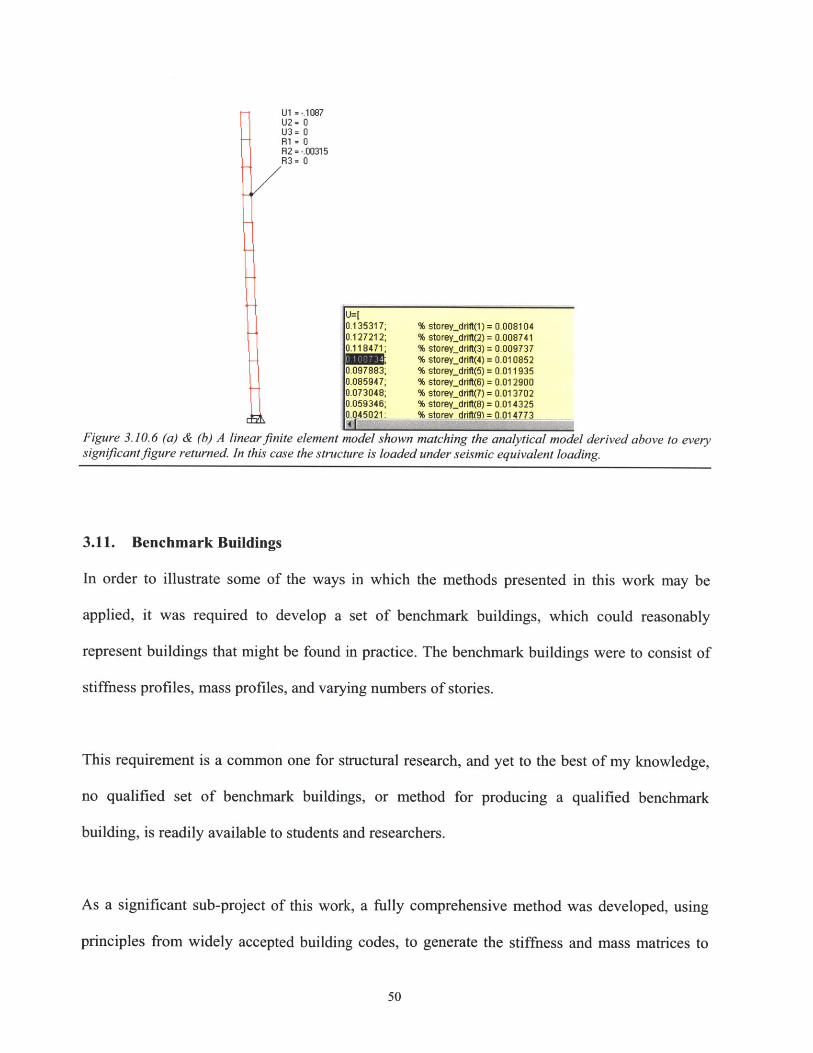
U1 =-.1087U2- 0U3= 0R1 = 0R2 = -.00315R3= 0
U=[0.135317, % storeydrift(1) = 0.0081040.127212; % storeydrilt(2) = 0.0087410.118471; % storeydrif(3) = 0.009737
% storeydrmt(4) = 0.0108520.097883; % storey,_drl(5) = 0.0119350.085947; % storeydrifI(6) = 0.0129000.073048; % storeydrift(7) = 0.0137020.059346; % storeydrift(8) = 0.0143250.045021: % storev driff(g) 0.014773
Figure 3.10.6 (a) & (b) A linear finite element model shown matching the analytical model derived above to everysignificant figure returned. In this case the structure is loaded under seismic equivalent loading.
3.11. Benchmark Buildings
In order to illustrate some of the ways in which the methods presented in this work may be
applied, it was required to develop a set of benchmark buildings, which could reasonably
represent buildings that might be found in practice. The benchmark buildings were to consist of
stiffness profiles, mass profiles, and varying numbers of stories.
This requirement is a common one for structural research, and yet to the best of my knowledge,
no qualified set of benchmark buildings, or method for producing a qualified benchmark
building, is readily available to students and researchers.
As a significant sub-project of this work, a fully comprehensive method was developed, using
principles from widely accepted building codes, to generate the stiffness and mass matrices to
50
define benchmark buildings. Using that method, 56 benchmark buildings were developed,
ranging from 2 to 15 stories in height. These benchmark buildings were tested with 116 different
rocking wall configurations, and the rocking wall design graph, as shown in sections 4.4 - 4.6,
for each benchmark building was found.
The method of creating benchmark buildings, the data for the benchmark buildings generated,
and the associated rocking wall design graphs, may be found in Appendix B.
The intent of the tables in Appendix B is that an engineer implementing a rocking wall project
would be able to find a close approximation of the building under consideration, and in a matter
of minutes determine the approximate size and number of rocking' walls that would be
appropriate, and whether rocking wall retrofit would be appropriate at all.
It is seen from the tables, for example, that for the benchmark (and thus intended to be
representative) buildings of only two stories, there is no possible rocking wall configuration that
will reduce the maximum story drift. And many other similarly interesting conclusions may also
be drawn from the tables.
The entire sub-project relating to benchmark buildings is presented in Appendix B.
51
3.12. Software Implementation
Software has been developed which solves the entire process described in section 3.10, and
offers many functions that will be useful for structural engineers who are designing a rocking
wall installation, and also for those working on a standard design project.
The software developed finds the stiffness matrix of the building based on the stiffness
distribution and a single story stiffness, if available. Otherwise, the software finds the stiffness
matrix by extrapolation of the ASCE 7-05 code, given whatever information the engineer has
available, such as the number of stories and lateral load resisting system, or the measured natural
period of the building. In the process of finding the stiffness matrix, the software also determines
the natural mode. The software then determines the total stiffness matrix of the building-rocking
wall system, and the equivalent seismic loads including the additional inertia of rocking wall.
The software then incrementally increases the size of the rocking wall, finding the maximum
story displacement under seismic loading for each rocking wall size, and reports the minimum of
those story displacements, and the rocking wall size that causes it, providing the engineer with an
optimization technique.
In order to apply the seismic loads including the inertia of the rocking wall (which is critical to
finding the minimum story drift), the mass of the rocking wall is discretized. Figure 3.12.1
illustrates this, and also illustrates the point that the rocking wall may rotate, but the building
floors do not.
52
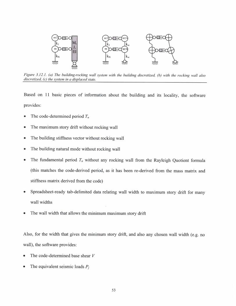
Figure 3.12.1. (a) The building-rocking wall system with the building discretized, (b) with the rocking wall alsodiscretized, (c) the system in a displaced state.
Based on 11 basic pieces of information about the building and its locality, the software
provides:
* The code-determined period Tn
* The maximum story drift without rocking wall
e The building stiffness vector without rocking wall
* The building natural mode without rocking wall
e The fundamental period T, without any rocking wall from the Rayleigh Quotient formula
(this matches the code-derived period, as it has been re-derived from the mass matrix and
stiffness matrix derived from the code)
* Spreadsheet-ready tab-delimited data relating wall width to maximum story drift for many
wall widths
* The wall width that allows the minimum maximum story drift
Also, for the width that gives the minimum story drift, and also any chosen wall width (e.g. no
wall), the software provides:
* The code-determined base shear V
e The equivalent seismic loads P
53

* The natural mode for the building with the rocking wall
" The total flexibility matrix including the rocking wall
* The forces in the links joining the building to the rocking wall
* The displacements of the structure under seismic equivalent loading, and the story drifts
" The story at which the maximum story drift occurs
All of the data is returned in MATLAB-ready syntax, which may be copied from the software,
should the engineer wish to perform further calculations with it.
RQCHIG-WA LCtM IRocking Wall Design
Introduction to Rocking Structures
The software presented here is illustrative software to
implement the ideas that emerged from a research projectinto rocking wall design. It is designed to provide a rockingFiurall 3.2.n,r Wesi withlr ative sftwr c*reat forA t i
Figure 3.12.2. Website with illustrative software created for this work
54

3.13. Software to Implement ASCE 7-05 Equivalent Seismic Loads
Through careful interpretation of the ASCE 7-05 code, it was possible to develop software that
would accurately determine the equivalent seismic loads for any given structure. It was vital to
develop this independently, firstly since it would be the foundation for developing further
software that would automate the process of applying those loads to structures. In addition, the
code is highly complex, and it is very easy to make mistakes in its application. For example, a
popular online calculator tool, by Buildings Guide6 6 , makes an error in determining the
approximate period of the structure. In applying the formula:
Ta = CTh; (3.7567)
that calculator neglects the fact that the above formula is only for moment frame systems, not for
shear wall systems,68 even though that calculator's default setting is a shear wall system. The
ASCE code does give the formula for calculating the approximate period for a shear wall
building, but it is complex, requiring summation terms. Another common mistake is to use the
geographical short period acceleration S, for buildings under six stories tall, but the code requires
a fixed S, of 1.5 in that case. The software developed for this work takes all of these factors into
account, and allows for up to 19 shear walls (the limitation is only there to prevent the interface
from being too large).
16 Buildings Guide (2012)
6 7 ASCE (2006), p 12 968ASCE (2006), p129
55
IOpen Pa" with assLts for coing
Scroll Dowfor Now Inputs
NMber ofStories
Told Storey Whobse& (R!
Tjlpe of LLRS IMoment Frame: Conrt
ElfecUw Selsmic Wli 200
Response ModMcanon Factor F
Occupancycatego 3 eg 300 peple.1-1.25
Log-pero Transiion Period
McE parameter Si()F=5
- 1-1
Ih....nmetres = 36.0; % total height (in)1h nrmetres = 36.0; % total height (m)
W= 200.0; % eff. selsmic weight (MN)
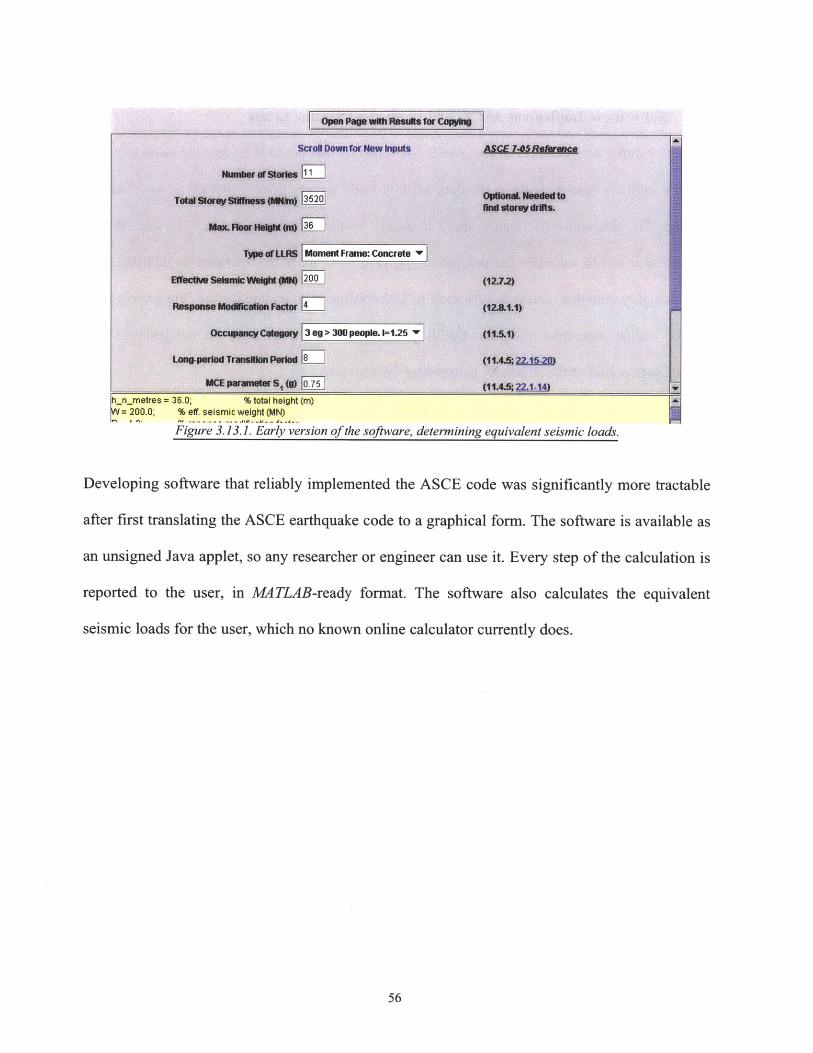
Figure 3.13.1. Early version of the software, determining equivalent seismic loads.
Developing software that reliably implemented the ASCE code was significantly more tractable
after first translating the ASCE earthquake code to a graphical form. The software is available as
an unsigned Java applet, so any researcher or engineer can use it. Every step of the calculation is
reported to the user, in MATLAB-ready format. The software also calculates the equivalent
seismic loads for the user, which no known online calculator currently does.
56

4. Analysis of Rocking Wall Design
4.1. Natural Frequencies of the Simulations
The analytical model with flexible wall using assumed modes, given in section 3.6, solved with
MATLAB code given in Appendix C, using a rocking wall with the dimensions used in the case
study retrofit (14.4ft wide by 2ft deep, as shown in section 2.5), and a two-story test model,
produces a period of 0.363s for the first natural mode, and 0.0106s for the second natural mode.
The finite element model, with SAP2000 used to perform the calculations, produces a period of
0.369s for the first natural mode, and 0.0181s for the second natural mode, for the same model.
The analytical model thus produces a first period that is only 1.7% less than the finite element
model, and a second period which is 41% less than the finite element method.
It should be expected that the first mode is the most accurate for the analytical model, since
currently only two trial modes have been applied to the system. As the number of trial modes is
increased, the accuracy of the higher modes improves. 69
A natural period within 1.7% of the finite element model is a very good start to the modelling
process. The accuracy of this result is an indicator that the analytical model is good and that
appropriate trial modes were chosen to represent the system.
69 Chopra (2006)
57

4.2. Natural Frequencies of the System With and Without Rocking Wall
The analytical model without the rocking wall, solved in MATLAB, procuces natural periods of
0.33118s, and 0.13718s for the two story test model. The finite element model produces natural
periods of 0.33117s, and 0.13718s for the same model. This virtually exact match should be
expected, and confirms that the basic principles of the analytical model are good.
As expected, adding the rocking wall increases the period of the first mode by 11%, making the
structure less stiff in that mode, while decreasing the period of the second mode (considering the
finite element result) by a notional 87%, making the structure much stiffer in that mode. Both of
these effects are generally good for the seismic response of a building, as illustrated infigure 1.3.
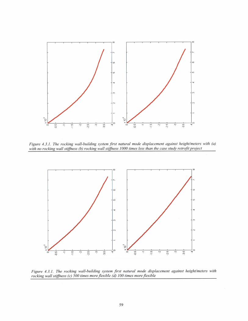
4.3. Modes of the System with Varying Stiffness of Rocking Wall
The stiffening effect of the rocking wall on the fundamental mode may be illustrated by solving
the analytical model using the MATLAB code in Appendix C, and finding the modes of the
system quantitatively, with varying stiffness of rocking wall, and with the rocking wall removed
entirely. The following figures illustrate these results for the first mode of the same two-story test
model.
58
(N
0 U? -7 1? LP If 0~ C) LP r U ? P
Figure 4.3.1. The rocking wall-building system first natural mode displacement against height/meters with (a)with no rocking wall stiffness (b) rocking wall stiffness 1000 times less than the case study retrofit project
LP - In PI C) IC) ( C')
CD In - P rn (N IP C In-0 7 r C?
Figure 4.3.1. The rocking wall-building system first natural mode displacement
rocking wall stiffness (c) 500 times more flexible (d) 100 times more flexibleagainst height/meters with
59
0
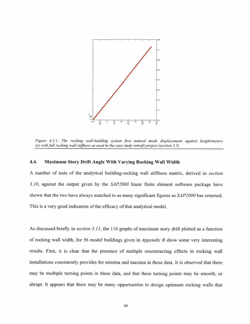
Figure 4.3.1. The rocking wall-building system first natural mode displacement against height/meters(e) with full rocking wall stiffness as used in the case study retrofit project (section 2.5)
4.4. Maximum Story Drift Angle With Varying Rocking Wall Width
A number of tests of the analytical building-rocking wall stiffness matrix, derived in section
3.10, against the output given by the SAP2000 linear finite element software package have
shown that the two have always matched to as many significant figures as SAP2000 has returned.
This is a very good indication of the efficacy of that analytical model.
As discussed briefly in section 3.11, the 116 graphs of maximum story drift plotted as a function
of rocking wall width, for 56 model buildings given in Appendix B show some very interesting
results. First, it is clear that the presence of multiple counteracting effects in rocking wall
installations consistently provides for minima and maxima in these data. It is observed that there
may be multiple turning points in these data, and that these turning points may be smooth, or
abrupt. It appears that there may be many opportunities to design optimum rocking walls that
60
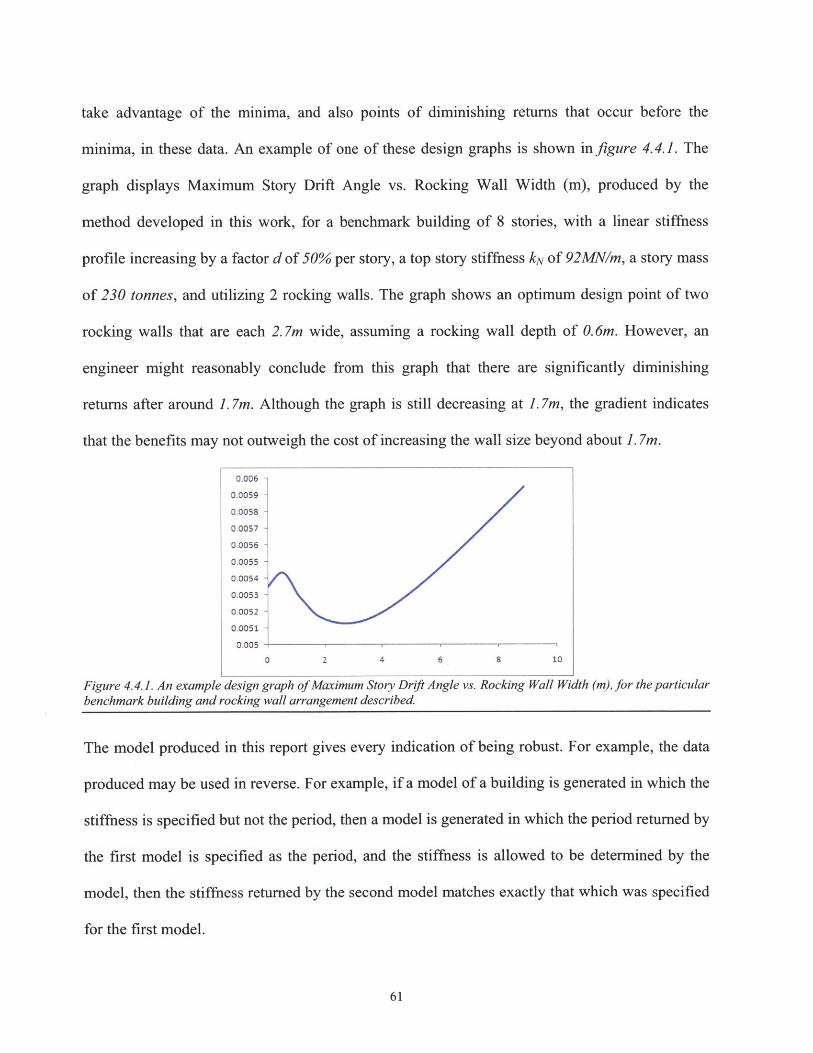
take advantage of the minima, and also points of diminishing returns that occur before the
minima, in these data. An example of one of these design graphs is shown infigure 4.4.1. The
graph displays Maximum Story Drift Angle vs. Rocking Wall Width (m), produced by the
method developed in this work, for a benchmark building of 8 stories, with a linear stiffness
profile increasing by a factor d of 50% per story, a top story stiffness kN of 92MN/m, a story mass
of 230 tonnes, and utilizing 2 rocking walls. The graph shows an optimum design point of two
rocking walls that are each 2.7m wide, assuming a rocking wall depth of 0.6m. However, an
engineer might reasonably conclude from this graph that there are significantly diminishing
returns after around 1. 7m. Although the graph is still decreasing at 1. 7m, the gradient indicates
that the benefits may not outweigh the cost of increasing the wall size beyond about 1. 7m.
0.006 -
0.0059 -
0.0058 -
0.0057 -
0.0056 -
0.0055 -
0.0054 -
0.0053 -
0.0052 -
0.0051 -
0.005
0 2 4 6 8 10
Figure 4.4.1. An example design graph of Maximum Story Drift Angle vs. Rocking Wall Width (m), for the particularbenchmark building and rocking wall arrangement described.
The model produced in this report gives every indication of being robust. For example, the data
produced may be used in reverse. For example, if a model of a building is generated in which the
stiffness is specified but not the period, then a model is generated in which the period returned by
the first model is specified as the period, and the stiffness is allowed to be determined by the
model, then the stiffness returned by the second model matches exactly that which was specified
for the first model.
61

4.5. Forces Applied to the Building by the Rocking Wall Inertia
By applying the model derived in section 3.10, the total maximum force in the building-rocking
wall links, under the code-specified seismic loading, is found to be approximately 8.2MN, or
1800 kips, for the case study building, occurring at the top story. This force is due to the inertia
of the building combined with that of the heavy rocking wall, and can be thought of as the effect
of the rocking wall trying to straighten the deformation of the building, while the building is
trying to bend under the lateral loading. This total load is distributed between 6 rocking walls
each with 2 lateral connectors per story, resulting in a maximum undamped load of about 680kN,
or 150kips per connector. However, the connections to the static shear walls, at the ends of the
building, are less stiff than the others are, so should be considered as attracting less load.
10 0
0
8 -
0
6 0
0
4 0
0
2 0
-8000 -6000 -4000 -2000 0 2000 4000 6000 8000Force in link (kN)
Figure 4.5.1. The forces in the building-rocking wall links, under code specified seismic loading, for the case studybuilding, as predicted by the static equivalent method presented.
This is a useful figure, since it illuminates the loading on the rocking wall itself, and thus could
allow further optimization of the rocking wall stiffness along its length.
62
At the lower stories, the wall is pushing the building further than it would ordinarily go under
this loading, to maintain the straight profile. Around the middle stories, the force in each link is
low. This can be thought of as being due to the natural position of the building under this
loading, approximately matching the wall-reinforced position, at that location. At the higher
stories, the wall is pulling the building back, less far than it would ordinarily go, to maintain the
straight profile. At the top story, the wall is once again pushing the building further than it would
go. This is due to the half-story mass associated with the top story in the model, and since the
seismic load is correlated with mass, the top story drift would usually be lower than other story
drifts. The top story drift is then forced to the near-constant story drift by the rocking wall.
One design strategy for a rocking wall, and later a rocking column, may be to design the wall or
colunm to stop short of the top story, if the weight of the top story were low, since otherwise the
wall may actually be applying greater stress to that story than is necessary.
The maximum link force is of the order of magnitude of the total weight of a story, and may also
be equated to the thrust produced by a jet engine, by order of magnitude. As discussed
previously, this figure is an upper bound, due to not taking account of supplemental damping.
Section 5 contains an analysis of whether the case study structure was sufficient to sustain these
lateral forces.
63

4.6. Comparison with Given Case Study Building Data
The team who designed the case study rocking wall installation were kind enough to share the
actual case study building data to aid with this work. It has thus been possible to compare the
simulation against experimentally confirmed data.
If the discretized case study story stiffnesses for each of the 11 stories is plotted against a linear
stiffness form where the incremental increase of the top stiffness is d=0.25, a very reasonable
match is found:
2-- Case
1.8 Model
1. -
1.1
0.8-
0.6
1. 2 3 4 5 6 7 8 9 10 11Story
Figure 4.6.1. The actual case study building story stiffnesses compared to a linear model.
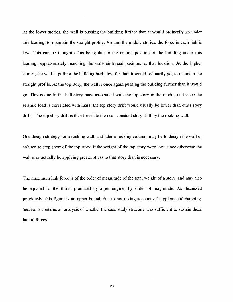
The mass model that has been used divides the total mass by the number of stories, and
distributes the mass equally between the stories, except for the top floor, to which it apportions
half the mass of the other floors. The comparison with the real case study data is again
reasonably good:
64
2500- -MW- Case-$ Model
20001
S 1500 --
1000 -
500 -
1 2 3 4 5 6 7 8 9 10 11Story
Figure 4.6.2. The given case study building story masses compared to a linear top-light model.
However, the mass model presented here (Fig 4.6.2, green dots) may be a more accurate
discretization of the case study building, as the mass for the top floor given by the case study
design team appears to be the combined mass of that floor, which is not the commonly accepted
method of building discretization.70
The actual value for natural period in the building x direction was given as 0.589s, and this is
confirmed to 2 decimal places by applying the iterated Rayleigh quotient formula to the given
information of stiffness and mass.
In a further illustration of robustness, if this given period of 0.589s is inputted into the formulae
developed for this work (as in Appendix B), using a stiffness increase factor d=0.25 as infigure
4.6.1, the stiffhesses generated are a reasonable approximation of the actual, with kN just 15%
less than the actual given value for kN.
70 Kausel (2010)
65
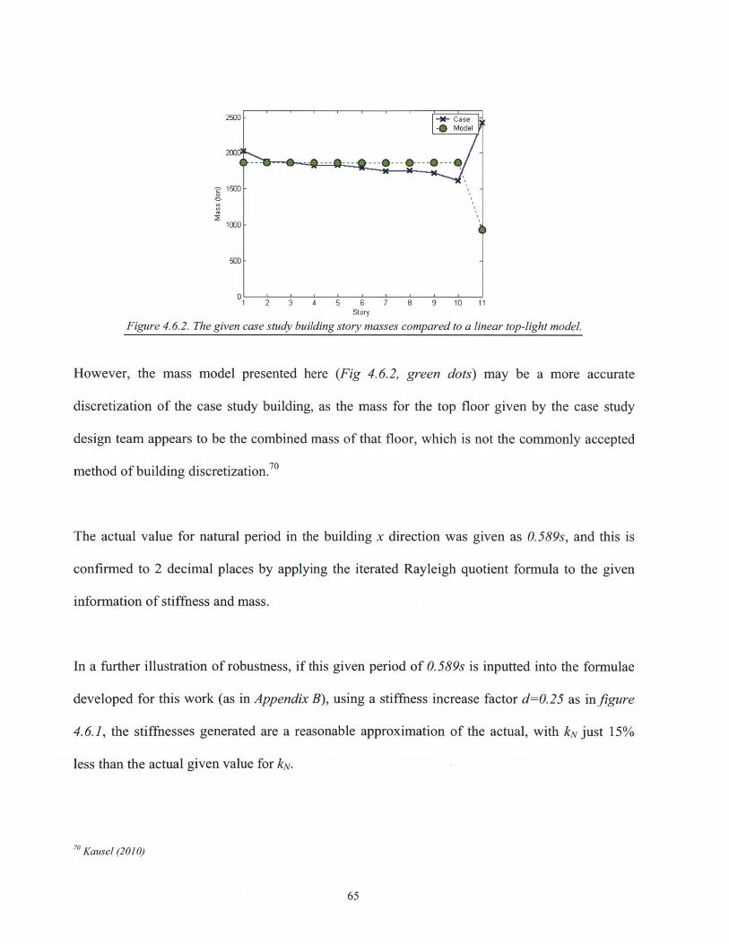
Similarly, given the true kN and a factor d=0.25, the linearized model developed provides a first
period of 0.539s, which is just 8.7% less than the period given. Applying this closely-matching
model of the case study building, and using six rocking walls with a wall depth of 0.61m, a top
story stiffness of 4.68GN/m, a user-specified stiffness profile of d=25%, applying the factored
earthquake intensity parameters for Tokyo71 , considering an effective seismic weight W of
200MN, 11 stories of 3.27m each, and a natural period of 0.589s, the following design graph,
tailored for the case study building, is found.
4.3
4.2
E
3.8-
0 2 4 6 8 10 12 14 16 18 20Wall Width (m)
Figure 4.6.3. The Rocking Wall Design Graph for the case study building, showing maximum story drift angle of themodeled case study building, against rocking wall width (m), using 6 rocking walls. The location of the 4.39m-widewalls actually used in the case study is marked.
It is seen fromfigure 4.6.3, that based on the design graphs produced by this analysis method,
the 4.4m-wide walls, that were chosen through an exhaustive experimental testing process, were
a highly appropriate choice for the case study building retrofit project. Although the actual
optimal minimum of the data is at 6.7m, it is seen from the figure that the returns obtained for
adding further wall size begin to diminish significantly after around 4.5m.
71 Kinetics (2008)
66

The fact that the suggested wall size given by the method presented in this work matches closely
that chosen for a fully experimentally-tested rocking wall installation is a useful confirmation of
this method.
It is thus clearly seen, that the models developed in this work suggest that for example 2m-wide
walls, or 12m-wide walls, would actually make the case study building's seismic response worse,
rather than better. This is a counter-intuitive, and thus very useful result.
It is also interesting to note that in this case the maximum story drift occurs at the sixth story
from the ground. Although some might expect the highest building stresses due to environmental
loads to always be at ground level, the maximum story drift only occurs at the lowest story in the
case where the story stiffness profile is close to constant. When the story stiffnesses are linearly
increasing, the maximum story drift due to the seismic equivalent loading often occurs as the
middle stories, according to the data produced by this model, as shown infigure 4.6.4. Since it is
usually seen in practice that buildings fail at a middle story during an earthquake, this is another
useful confirmation that the equivalent seismic loading method used here is a good tool to
predict and prevent such middle story failure. If the correct parabolic stiffness were used, then
the drift profile under seismic loading would be linear 72, and thus optimal, as previously
discussed.
72 Connor (2003)
67

X 103
3.8
3.7 X
3.6 x
3.5-
3.4 X
3.2
3.1 X
3-
2.9-
2.81 2 3 4 5 6 7 8 9 10 11
Story
Figure 4.6.4. The story drift angles of the case study building under seismic equivalent loading, with the maximumoccurring at the middle stories.
Another helpful result is that the output design parameter of the method presented is especially
robust. If the story stiffnesses or masses are changed by some reasonable amount, the overall
shape of the graph remains very similar, with very little movement of the minimum or the point
of diminishing returns, as shown in figure 4.6.5. And so although a number of approximations
have been incorporated to the model of the building (figures 4.6.1 - 4.6.2), there can be
confidence that the result returned for most useful size of rocking wall would be very similar
even if the fully analytical mass and stiffness matrix of the building had been used. The same is
true if the loads are scaled, for example by changing the location of the building and thus the
magnitude of the equivalent seismic loads. Thus it appears that the primary aim of this work,
which was to offer a useful starting point for rocking wall size for rocking wall installations, has
been achieved.
68

x 103
3.4
0 23.8 1 2 1 1 8 2
Wall Width (m)
Figure 4.6.5. The rocking wall design function of the case study building compared to cases where all storystiffnesses are modified by ±10%. The central line is the case study, the upper with stiffnesses decreased by 10%,and the lower with stffnesses increased by 10%. The change in the minimal width 3 is only 0.2m, illustrating therobustness of the output.
69

5. Study to Determine whether the Case Study Rocking Wall Caused
Damage During the Thhoku Earthquake
Figure 5.0.1. The case study building model, as retrofitted with rocking walls. The arrow indicates a static shear
wall that was damaged during the 2011 earthquake, which was of relatively light intensity in Tokyo.
It is noted during the Tohoku Earthquake of March 2011, that a shear wall adjacent and
perpendicular to the case study rocking wall installation was damaged. Based on the work
culminating with section 4.5, which suggests very high inertial forces from the rocking wall, it is
theorized that the inertial forces exerted by the adjacent rocking wall were responsible for the
damage to the static shear wall. The inertial forces that rocking walls exert on surrounding
structure will be studied, and it will be demonstrated that the stresses experienced by the static
shear wall due to the rocking wall inertial forces were sufficient to cause the damage that was
observed.
70
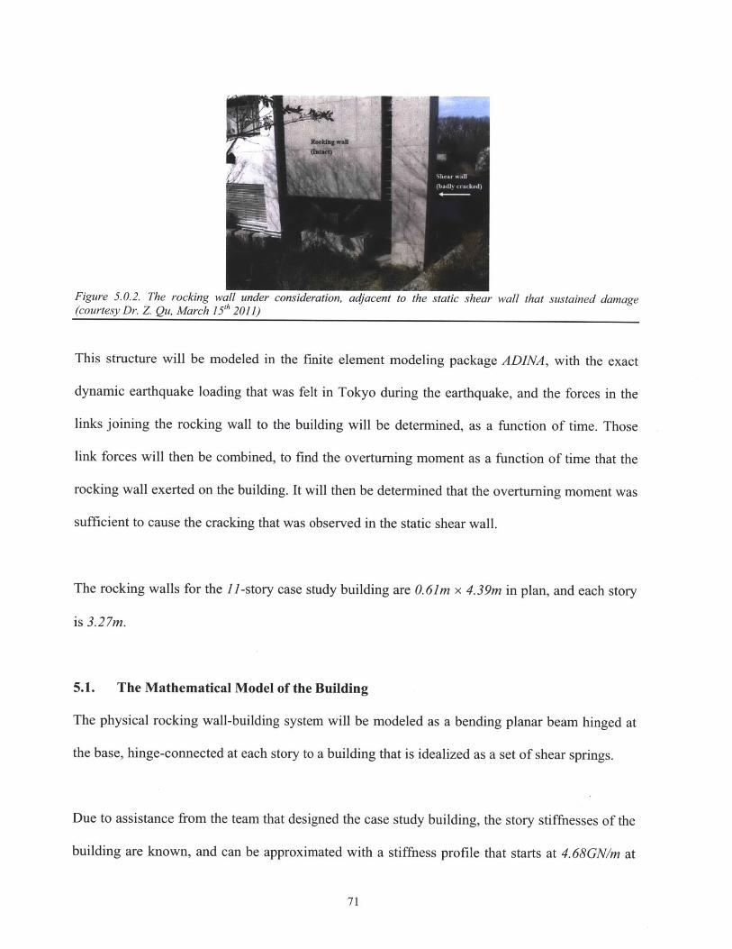
Figure 5.0.2. The rocking wall under consideration, adjacent to the static shear wall that sustained damage(courtesy Dr. Z Qu, March 15 h 2011)
This structure will be modeled in the finite element modeling package ADINA, with the exact
dynamic earthquake loading that was felt in Tokyo during the earthquake, and the forces in the
links joining the rocking wall to the building will be determined, as a function of time. Those
link forces will then be combined, to find the overturning moment as a function of time that the
rocking wall exerted on the building. It will then be determined that the overturning moment was
sufficient to cause the cracking that was observed in the static shear wall.
The rocking walls for the 11-story case study building are 0.61m x 4.39m in plan, and each story
is 3.27m.
5.1. The Mathematical Model of the Building
The physical rocking wall-building system will be modeled as a bending planar beam hinged at
the base, hinge-connected at each story to a building that is idealized as a set of shear springs.
Due to assistance from the team that designed the case study building, the story stiffnesses of the
building are known, and can be approximated with a stiffness profile that starts at 4.68GN/m at
71
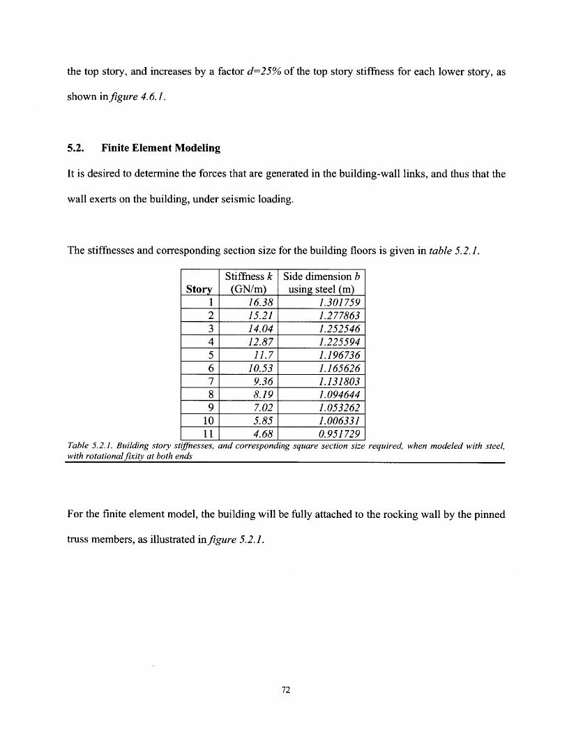
the top story, and increases by a factor d=25% of the top story stiffness for each lower story, as
shown infigure 4.6.1.
5.2. Finite Element Modeling
It is desired to determine the forces that are generated in the building-wall links, and thus that the
wall exerts on the building, under seismic loading.
The stiffnesses and corresponding
Story123456789
1011
Table 5.2.1. Building story stiffnesses, awith rotational fixity at both ends
section size for the building floors is given in table 5.2.1.
Stiffness k Side dimension b(GN/m) using steel (m)
16.38 1.30175915.21 1.27786314.04 1.25254612.87 1.225594
11.7 1.19673610.53 1.165626
9.36 1.1318038.19 1.0946447.02 1.0532625.85 1.0063314.68 0.951729
nd corresponding square section size required, when modeled with steel,
For the finite element model, the building will be fully attached to the rocking wall by the pinned
truss members, as illustrated infigure 5.2.1.
72
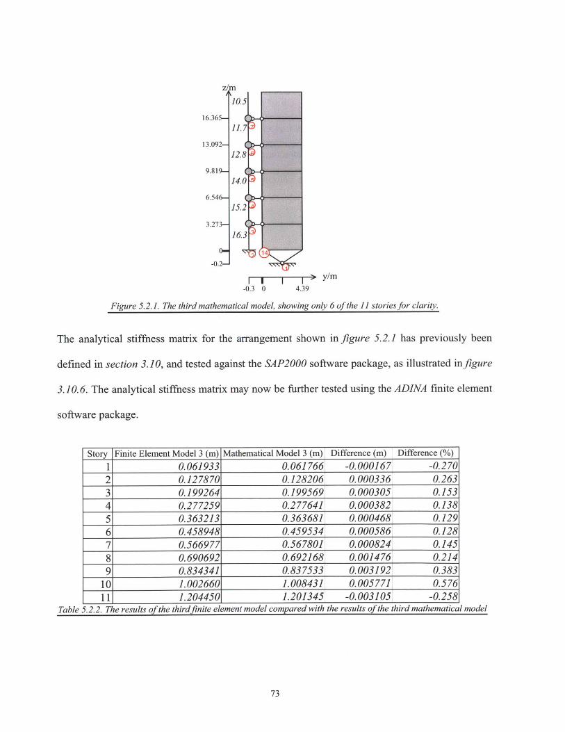
16.3(
13.
I I 1 1-- y/m-0.3 0 4.39
Figure 5.2.1. The third mathematical model, showing only 6 of the 11 stories for clarity.
The analytical stiffness matrix for the arrangement shown in figure 5.2.1 has previously been
defined in section 3.10, and tested against the SAP2000 software package, as illustrated infigure
3.10.6. The analytical stiffness matrix may now be further tested using the ADINA finite element
software package.
Story Finite Element Model 3 (m) Mathematical Model 3 (m) Difference (m) Difference (%)
1 0.061933 0.061766 -0.000167 -0.2702 0.127870 0.128206 0.000336 0.2633 0.199264 0.199569 0.000305 0.1534 0.277259 0.277641 0.000382 0.1385 0.363213 0.363681 0.000468 0.1296 0.458948 0.459534 0.000586 0.1287 0.566977 0.567801 0.000824 0.1458 0.690692 0.692168 0.001476 0.2149 0.834341 0.83 7533 0.003192 0.383
10 1.002660 1.008431 0.005771 0.57611 1.204450 1.201345 -0.003105 -0.258
73
Table 5.2.2. The results of the thirdfinite element model compared with the results of the third mathematical model

The maximum difference in the results between the finite element model and the mathematical
model is 0.6%, but are mostly around 0.2%. Clearly this is a very good match. The reason for the
slight difference is that the version of ADINA used is limited to 900 finite element nodes. While
SAP2000 performs all element meshing automatically, meshing is chosen by the engineer in
ADINA to allow the engineer to optimize complex problems, and in the version available is
limited to 900 nodes.
To fully compare the analytical stiffness matrix against the finite element model, the stiffness
matrix can be found directly from the finite element model by setting each degree of freedom to
unity in turn, while holding the others fixed and finding the reactions will give one row of the
stiffness matrix. However this is a laborious process to accomplish by hand, and checking the
displacements in this way is sufficient.
The model includes 2-D elements, which only approaches the exact theoretical solution as the
number of elements increases. 73
7 Bathe (1996)
74
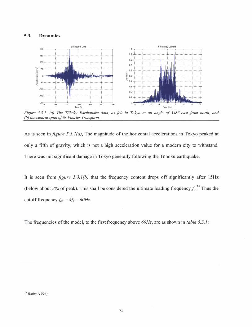
5.3. Dynamics
20
160
100
50
0
-50
-100
-150
Earthquake Data
--- -- -r-- -- - -- r - - -- - -- --- -- - -- - -- -- - -- -- -- -- - --
-- - -- - - - ---- --- -- --- --- -- -- -- --- -- ----
-- -- - ------- ---- -------- -------- I--------
---- ---- ------------ -------- -------_
0 50 100 150 2W 250 300Time (s)
Figure 5.3.1. (a) The Tjhoku Earthquake data, as(b) the central span of its Fourier Transform.
felt in
Frequency Content
1
0.9 -- - ------- --- - ----- - - - - - - - - - - -
0.7 ---------- ------- ------ ----- ------ ---------70.6 ------ ----- -- -- - ---- -- -- ------ -
0.5 ------ ------ --- -- -------
0.4 ------ ------------- ------ ------ - -----
0.2 ------ ------ ----- - '----- ------
0.1 - -- -- - -- - -- -- -
0 20 -15 -10 -5 0 5 10 15 20Freq (Hz)
Tokyo at an angle of 3480 east from north,
As is seen in figure 5.3.1(a), The magnitude of the horizontal accelerations in Tokyo peaked at
only a fifth of gravity, which is not a high acceleration value for a modem city to withstand.
There was not significant damage in Tokyo generally following the Tohoku earthquake.
It is seen from figure 5.3.1(b) that the frequency content drops off significantly after 15Hz
(below about 3% of peak). This shall be considered the ultimate loading frequencyf,. Thus the
cutoff frequency fco = 4f, = 60Hz.
The frequencies of the model, to the first frequency above 60Hz, are as shown in table 5.3.1:
74 Bathe (1996)
75
and
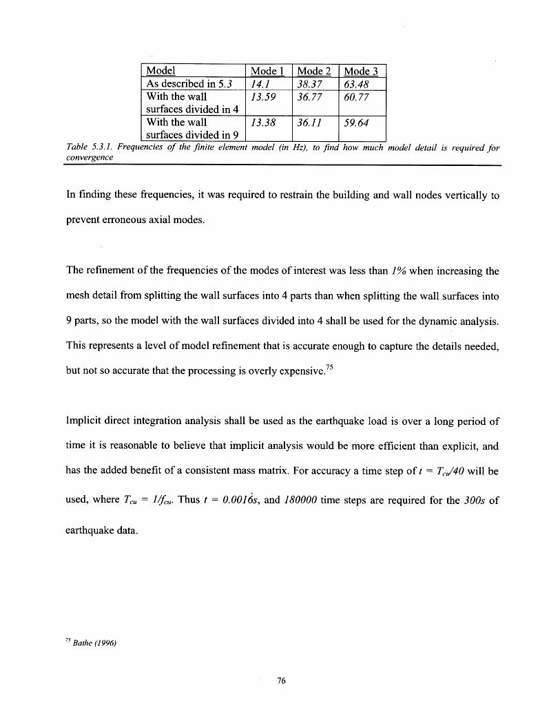
Table 5.3.1. Frequencies of the finite elementconvergence
model (in Hz), to find how much model detail is required for
In finding these frequencies, it was required to restrain the building and wall nodes vertically to
prevent erroneous axial modes.
The refinement of the frequencies of the modes of interest was less than 1% when increasing the
mesh detail from splitting the wall surfaces into 4 parts than when splitting the wall surfaces into
9 parts, so the model with the wall surfaces divided into 4 shall be used for the dynamic analysis.
This represents a level of model refinement that is accurate enough to capture the details needed,
but not so accurate that the processing is overly expensive.75
Implicit direct integration analysis shall be used as the earthquake load is over a long period of
time it is reasonable to believe that implicit analysis would be more efficient than explicit, and
has the added benefit of a consistent mass matrix. For accuracy a time step of t = Te./40 will be
used, where Te,, = 1/fe. Thus t = 0.0016s, and 180000 time steps are required for the 300s of
earthquake data.
7s Bathe (1996)
76
Model Mode 1 Mode 2 Mode 3As described in 5.3 14.1 38.37 63.48With the wall 13.59 36.77 60.77surfaces divided in 4With the wall 13.38 36.11 59.64surfaces divided in 9 1 1
However, this many time steps produces an 8.6GB ADINA porthole file, which the software
cannot open on the computer hardware available. In ADINA, the number of time steps recorded
can be limited by going using the function Control/Porthole/Timesteps (nodal results), setting
the function to Overwrite Any Existing Blocks, and defining all of the 180000 time steps as being
in one of these 'blocks'. The period of interest in the earthquake is 75s to 150s, which
corresponds to time steps 45000-90000. Additionally, it is chosen to not record any time steps
for the blocks outside of this period, and only one in six time steps will be recorded for this
period, which is one every 1 /1 0 0 th of a second, the frequency of the acceleration data.
5.4. Units and Consistency
The acceleration load is applied in m/s 2, which is the consistent unit for SI, which the model has
been constructed in. The acceleration loads that are to be used are for Tokyo, which was far from
the epicenter of the Tohoku earthquake. As such, this data is not high-priority and has not been
processed, and has a non-zero mean. This means that in the video illustration of the finite
element analysis, the building can be observed drifting to one side. Japan of course is known to
have moved by 8 feet in the Tohoku earthquake, and so to some degree that motion accurately
represents the history, although drift observed in the illustration is greater than the 8 feet that
Japan is commonly understood to have moved during the earthquake. This fact is not detrimental
to the present analysis, in which it is planned to find the forces in the links between the building
and the rocking wall. Since the movement is gradual over 5 minutes, the accuracy of the link
forces will not be significantly affected.
77
5.5. Mass for Dynamic Analysis
Mass will be added to the finite element model at specific points, in particular 2000 tonnes will
be added at points 3 to 12, and 1000 tonnes at point 13, to match the mathematical model of the
building. This is accomplished in ADINA with the function Model/Element
Properties/Concentrated Masses. In addition, the material that the building was notionally
constructed in the finite element model from has its density set to zero, matching the
mathematical model of a lumped-mass building.
5.6. Finding and Processing the Link Axial Forces in ADINA
To find the axial forces in each link (represented in the finite element model by lines 48 to 58),
each one must be added to a different element group (element groups 14 through 24), as although
setting the zone to "element 1 of element group 2" and so on was accepted by ADINA as correct
syntax, it did not function as expected. On time steps after the first, details for other elements
were also printed. Also it was not immediately apparent which element was element n.
To solve that problem, the data were processed with text editing software to obtain 11 vectors of
forces in MA TLAB-ready syntax. These vectors were then multiplied by the height vector for the
structure, and the results summed, to find the combined .turning moment at the base of the
building, as a function of time. The result is shown infigure 5.6.1, below.
78

x 108
6-
4
Ez
E0 2-2
-4-
-6-
70 80 90 100 110 120 130 140 150Time (s)
Figure 5.6.1. The overturning moment at the base of the building, as afunction of time
5.7. The Addition of Damping to the Model
For the final model, 5% Rayleigh Damping was added in ADINA using the commands
Control/Analysis Assumptions/Rayleigh Damping, and setting the parameters a and 8 to 0.7225
and 1.67E-3 respectively.
As is seen fromfigure 5.7.1, the addition of 5% damping to the model reduced the peak moment
by nearly 30%, and the sustained moment magnitude by even more.
79

x 108
4 -
2 -
E 0-
-2-
-4
70 80 90 100 110 120 130 140 150Time (s)
Figure 5.7.1. The overturning moment at the base of the building, as afunction of time, with 5% Rayleigh damping
5.8. Calculation of the Static Shear Wall Cracking Moment
The size of the static shear wall as seen infigure 5.0.2 is approximately 5.2ft by 54.4ft, and thus
the second moment of area of the weak axis is 637.42 ft4 . High strength 5 ksi concrete is
assumed.
The cracking moment may be found from the following formulae:76
fr = 7.5 4fc = McrackYmax/I (5.1)
Merack = 7.5I4f'c/ymax (5.2)
76 Nilson et aL. (2009)
80

It is found that the cracking moment of the static shear wall is 2.247x]08 lb-in or 2.5393x]07
Nm. The first moment value recorded in the high-energy earthquake period from 75s to 150s is
4.8x1 07 Nm, almost twice the cracking moment. Thus it is seen that the cracking strength of the
concrete was reached relatively early in this earthquake. The remaining earthquake cycles over
the following minutes will have continued to crush the concrete around the cracks, making the
cracks visible to the naked eye, as was observed. The peak overturning moment, approximately 2
minutes into the earthquake, was approximately 20 times the cracking moment of the static shear
wall.
5.9. Conclusions of the Finite Element Study
It is clear from the finite element analysis presented that the inertia force from the rocking wall
was sufficient to cause, and most likely was the cause of the cracking in the adjacent static shear
wall of the building studied.
The high inertial forces generated by rocking walls during an earthquake should be carefully
considered by designers implementing this scheme. In this particular case, the rocking wall
should not be attached to the static shear wall, and the static shear wall should not block the
dynamic path of the rocking wall.
Connections from a rocking wall to a building should only be on the near side of the rocking
wall, when the rocking wall is constructed on the edge of a building.
81

It may be noted that while the loads imposed by the rocking wall were substantial, they were not
entirely unmanageable. Equations 5.1 - 5.2 show that if the static shear wall were doubled in
thickness, it could have sustained the loads without cracking.
82

6. Rocking Column Design
6.1. Rationale for Design
As a consequence of the research presented in this work, it has become apparent that the lateral
inertial forces exerted by rocking walls on the surrounding structure during an earthquake are
greater than was previously understood.
In addition to requiring additional care in the design process, regarding the kind of adjacent
structures that should be supporting the inertial lateral loads from rocking walls, it emerges
clearly from the presented research that when under full code-specified seismic loading, the total
maximum load that rocking walls apply laterally is of the magnitude of one story weight. For the
case study building presented, this total maximum lateral load occurs at the top story, and is
8.2MN, or 1800 kips in magnitude, which is 4 times more than the weight of the rocking wall
itself. It is clear that the connections from the rocking wall to the building are required to be very
significant to support such a load. Such connections are not readily available, and are costly. And
although this load is the maximum load, the loads at other stories are also significant.
The above loads were calculated without the effect of supplemental damping systems, and so
should be considered an upper bound. However, it would not generally be expected for even
optimum damping to reduce the lateral loads by more than 50%, and thus the remaining loads
will still be very difficult to control.
In addition, the foundations required for rocking walls, and the pins required at their base, are
very significant and costly. For the case study building, each of the six rocking walls are 3400
83

cubicfeet in volume, and 500 kips of weight, not including the case iron base. As a reference, the
case study retrofit project added 50% to the existing reinforce concrete area, in plan.
Clearly, reinforced concrete rocking walls have been a highly commendable academic effort, and
have taught the engineering community a lot about this kind of dynamic structure. However,
there are practical difficulties inherent in their design that must still be overcome.
6.2. Introduction to Rocking Column Design
It is suggested that to overcome the difficulties observed with rocking walls, that a structure be
designed from steel which maintains the desired properties of adding lateral stiffness to the
structure, while being moment-released at the base, but without the high mass of a rocking wall.
Starting from the assumption that a wide flange section is most efficient in general bending,
some initial calculations can be performed to determine the size of section that would be required
to replace, for example, a rocking wall from the case study:
IcEe = IsEs (6.1)
Ee = 2AJ42Es (6.2)
and thus:
bdEe bdAf= 6Es ~~0 (6.3)
where Ic, Is, Ec, Es are the strong second moment of area and modulus, of the concrete and steel
respectively, A4 is the area of the flange, and d, b are the dimensions of the rocking wall in plan.
84

Thus for the same stiffness, the total area of steel flange is 95% less than the area of concrete.
Steel is approximately 3.25 more dense than concrete, and so the weight of the steel flanges is
approximately 84% less than the weight of the concrete.
The web of the wide-flange section need not be continuous, but rather should most likely be
designed as a truss. In particular, a concentric braced frame, as illustrated in figure 6.2.1 is a
popular form of deep supporting section in steel construction. For total steel weight, a
reasonable conservative first estimate is that for the deep section considered for the case study
building, the web be an inch thick. Ultimately, the web design would be a much lighter truss of
course, so this would be a gross overestimate of the web area A,,. If applied consistently for any
size section, this would suggest a web area of:
bdA 2 ~ (6.4)
This upper bound estimate would then suggest a total steel area of 91% less than the equivalent
concrete system, and a total weight of 70% less. This corresponds to a rocking column weighing
approximately 150 kips, for the case study example, compared to the rocking wall with a weight
of 500 kips.
7 McCormac and Csernak (2012)
85

Figure 6.2.1. Schematic (a) lower elevation, and (b) plan, of a rocking column, with trussed web
6.3. Further Rocking Column Design
For the case study building, the flange size required is 104in2 , which is 4.3 in. wide over the 24
in. depth of the available space. Such sizes of steel plate are not commonly available.
One possible solution would be to build up a thicker section from thinner plates, which may be
desirable in certain architectural situations. Architectural considerations are addressed further in
section 6.5. The most realistic structural approach is to use a standard wide-flange or WT section
for the flange of the rocking column.
The most likely candidate wide flange sections for the case study example are given in Table
6.3.1.
86

Section Area A, in' Overall depth d. in flange width bf. in flange thickness tf in
W40x362 107 40.6 16.0 2.01W36x361 106 38.0 16.7 2.01W33x354 104 35.6 16.1 2.09W30x357 105 32.8 15.5 2.24W27x368 108 30.4 14.7 2.48W24x370 109 28.0 13.7 2.72Wl4x370 109 17.9 16.5 2.66
Table 6.3.1. Candidate wide flange sections for the flange of a rocking column for use in the case study building7 8 .
All shapes are considered heavy shapes, with a flange thickness greater than 2 ", so AISC A3. 1(c) applies.
The least wide section is most desirable, since it is required to get the rocking column flange area
as far from the middle of the rocking wall as possible. This requirement would lead to W24x370
being chosen. However, the depth of the section is 4 in. more than the current rocking wall.
Possibly this would be within tolerances. However, W14x370 will be chosen, with a web
thickness of 1.66 in., to ensure that the rocking column design would fit within the existing space
allocated for the rocking wall. This is illustrated in plan, to approximate scale, infigure 6.3.1.
I IFigure 6.3.1. A schematic plan of a rocking column, using standard structural steel wide flange shapes, designed for
the case study building, to approximate scale, assuming 4 in. members for the truss web.
An alternative approach would be to use a WT shape for the flanges. These are more expensive
per unit mass of steel, since they consist of a wide flange shape that has been cut in half along
the web, and are not as common as wide flange shapes. However, they would offer a more
efficient use of steel, since the steel would be as far as possible from the center of the rocking
column.
There are only two standard WT sections that meet the area requirement, as shown in table 6.3.2.
87

Section Area , in2 Overall depth d, in flange width br, in flange thickness t. in
WT18x400 118 21.3 18.0 4.29WT7x365 107 11.2 17.9 4.91
Table 6.3.2. Candidate WT sections for the flange of a rocking column for use in the case study building". Allshapes are considered heavy shapes, with aflange thickness greater than 2".
As is seen from table 6.3.2, the net effect of using a wide flange section for this purpose would
be simply to split the flange of the rocking column into two halves.
Both of the possible WT sections meet the depth requirement of 24 in. However, the WT7x365 is
the better choice in this case, with a flange thickness of 4.91 in., placing the maximum area away
from the center of the rocking column, and the lightest possible, with a stem thickness of 3.07 in.
This yields an ideal rocking column, as illustrated infigure 6.3.2.
Figure 6.3.2. A schematic plan of a rocking column, using standard structural steel WT shapes, designed for thecase study building, to approximate scale, assuming 4 in. members for the truss web.
6.4. Detail Design
The open-face cast iron pin presented by Wada et al., illustrated infigure 2.1.2 and pictured in
figure 6.4.1 is a proven design, behaving as intended during the 2011 earthquake. A smaller
version of that pin might be used for this purpose.
8 AISC (2005)" AISC (2005)
88
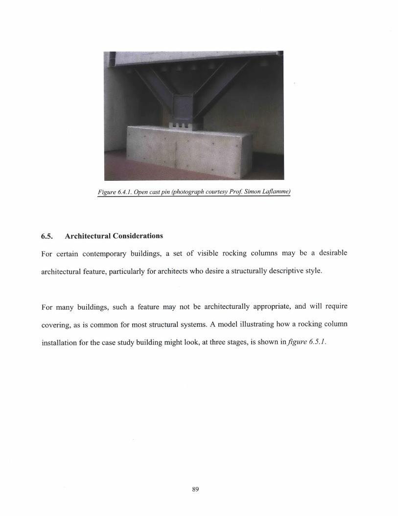
Figure 6.4.1. Open cast pin (photograph courtesy Prof Simon Laflamme)
6.5. Architectural Considerations
For certain contemporary buildings, a set of visible rocking columns may be a desirable
architectural feature, particularly for architects who desire a structurally descriptive style.
For many buildings, such a feature may not be architecturally appropriate, and will require
covering, as is common for most structural systems. A model illustrating how a rocking column
installation for the case study building might look, at three stages, is shown infigure 6.5.1.
89
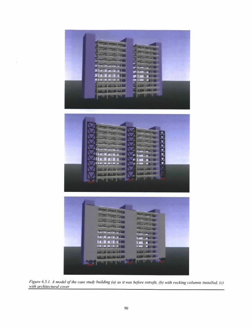
Figure 6.5.1. A model of the case study building (a) as it was before retrofit, (b) with rocking columns installed, (c)with architectural cover
90

6.6. Analysis of the Benefits of Rocking Columns
6.6.1 Lateral Force Reduction
The software developed for rocking wall analysis was modified to allow both rocking wall
analysis and rocking column analysis.
Based on a new full analysis of the case study building, it is found for the case study building
that the maximum lateral force in the wall-building links is projected to drop by 7.5% with a
rocking column, corresponding to the drop in mass of the new system.
The case study building is very massive, due to being long in one direction. The reduction in
lateral force from using a rocking wall is greater for a less massive building, since the rocking
wall represents a greater fraction of the total mass of the building. For a very massive building,
the majority of the lateral link load may be attributed directly to the action of the stiffness of the
rocking wall or column.
10- 0
8-e
6 0 0
2 0
-00 -6000 -4000 -2000 0 200 4000 6000 8000Force in link (kN)
Figure 6.6.1.1. The forces in the building-rocking column links, under code specified seismic loading, for the casestudy building, as predicted by the static equivalent method presented.
91
6.6.2 Foundations Reduction
As discussed in section 6.2, the weight of rocking columns is predicted to be 70% less than that
of rocking walls. It is thus reasonable to consider that the foundations required for rocking
columns will be 50% to 70% less substantial than those required rocking walls, with significant
cost savings.
6.6.3 Cost Effective Connections
As has been established, substantial lateral connections are required between the rocking wall
and the building, for either rocking walls, or rocking columns. Such connections are predicted to
be more cost effective for rocking columns, since steel-to-steel connections are significantly less
expensive than steel-to-concrete connections. 80
6.6.4 Greater Story Drift Reduction, with Potential for Further Reductions
As is seen from figure 6.6.4.1, since the use of steel rather than concrete reduces the system
density by 70%, a significant reduction in maximum story drift is achieved for the case study
building, using the same size column as the wall that was used: 4.39m wide by 0.61m deep.
80 McCormac and Csernak (2012)
92
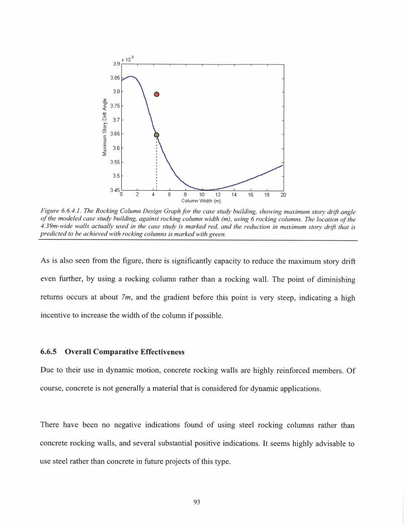
3.9
3.85 -
3.8 -
3.75 -
3.55 -3.65 '
EE
3.55 -
3.5 L
3.45'0 2 4 6 8 10 12 14 16 18 20
Column Width (m)
Figure 6.6.4.1. The Rocking Column Design Graph for the case study building, showing maximum story drift angleof the modeled case study building, against rocking column width (m), using 6 rocking columns. The location of the4.39m-wide walls actually used in the case study is marked red, and the reduction in maximum story drift that ispredicted to be achieved with rocking columns is marked with green.
As is also seen from the figure, there is significantly capacity to reduce the maximum story drift
even further, by using a rocking column rather than a rocking wall. The point of diminishing
returns occurs at about 7m, and the gradient before this point is very steep, indicating a high
incentive to increase the width of the column if possible.
6.6.5 Overall Comparative Effectiveness
Due to their use in dynamic motion, concrete rocking walls are highly reinforced members. Of
course, concrete is not generally a material that is considered for dynamic applications.
There have been no negative indications found of using steel rocking columns rather than
concrete rocking walls, and several substantial positive indications. It seems highly advisable to
use steel rather than concrete in future projects of this type.
93
7. Suggested Extensions
There is much that could be extended in this work. A number of possible extensions to this work
are suggested:
* Use the link forces to determine the stresses in the wall & thus indicate the amount of
pre/poststress required in the wall.
* Apply a dynamic load application approach to these issues.
* Consider that seismic damage to columns may decrease the story stiffnesses during an
earthquake.8 '
* Add to the software the ability to take an input of zip code and to derive the design spectral
acceleration values Ss and Si from the zip code.
* Add supplemental damping to the model, which the analytical model is designed to allow,
since it allows the wall to move independently from the building.
* Allow for a fully specified stiffness, mass, and height vectors in the software.
Koh et al. (1995)
94

8. Conclusions
Retrofitting certain sizes of rocking walls to older buildings is an effective method of reducing
structural response during a seismic event. It is thus an effective method of reducing the
structural damage caused, thus reduces the potential for loss of life and societal disorder.
Care must be taken in the rocking wall design process, however, to ensure that adjacent systems
are capable of supporting the high lateral loads that the rocking wall will exert during a seismic
event. Those forces are primarily due to the stiffness of the rocking wall, but also increase with
the mass of the rocking wall. In addition, as also shown in this work, care must be taken that
useful sizes of rocking wall are chosen, and not sizes that will worsen the structural response.
If the top story of a retrofitted building is significantly lighter than other stories, the research
presented implies that rocking walls and columns may be stopped short of the top story without
negative consequence.
Current rocking walls designs consume significant area on a building plan, and may not be the
most effective option for a modem newly constructed building that requires maximum available
light and access. However, the latest buildings use all available technologies to deal with extreme
load cases, and rocking walls may form part of a comprehensive damage reduction strategy for
new buildings, particularly if optimized rocking wall sizes for given applications can be
identified.
The quasi-static approach to applying seismic loads to structures is an effective way of
determining the maximum story drift when the building is excited in its first mode. The
frequencies of higher modes are increased significantly by rocking columns or rocking walls,
often well beyond excitation frequencies, reducing the need to analyse those modes.
95

The general stiffness matrix derived for a discretized shear spring-mass system pin-connected to
a flexible pinned column (a simplified building-rocking wall system) provides an accurate
description of the simplified building-rocking wall system under arbitrary loading.
The total maximum forces in the links joining the rocking wall to the building in the case of the
case study building rocking wall retrofit have an upper bound of the order of one story weight,
and occur at the top stories of an installation. Supplemental damping may reduce these forces.
The representative discretized building models presented are a useful tool by which to simulate
structural ideas against a broad background of representative buildings.
Based on comparison with the case study rocking wall retrofit, the method presented of using an
analytical model to produce a design graph of maximum story drift against rocking wall size is
an effective way to optimize the size of rocking wall required for a rocking wall installation
project.
The use of steel rocking columns, as presented in section 6, is an effective way to reduce the
difficulties associated with concrete rocking walls. They show evidence of reducing the
maximum story drift further than rocking walls for the same volume of wall, and have potential
for greater story drift reductions than rocking walls. They require smaller foundations, and
smaller lateral connections. Rocking columns have a greater potential to be commercially viable
than rocking walls have so far been.
96
9. References
Ajrab et al. (2004) Rocking Wall-Frame Structures with Supplemental Tendon Systems.
Available at: http://dx.doi.org/IO.1061/(ASCE)0733-9445(2004)130:6(895) (Accessed: 16 January 2012)
American Institute of Steel Construction (AISC) (2005) Specifications for Structural Steel
Buildings., ASCE/SEI 7-05.
American Society of Civil Engineers (ASCE) (2006) Minimum Design Loadsfor Buildings and
Other Structures, ASCE/SEI 7-05.
Bathe, K-J. (1996) Finite Element Procedures., Prentice-Hall
Buildings Guide (2012) Seismic Base Shear Calculator.
Available at: http://www.buildingsguide.com/calculators/structural/IBC2006E/ (Accessed: 16 January 2012)
Chopra, A. (2006) Dynamics of Structures., Prentice-Hall
Connor, J. (2003) Introduction to Structural Motion Control. Pearson Education, Upper Saddle
River
Deierlein, G. (2010) Presentation: Damage Resistant Braced Frames with Controlled Rocking
and Energy Dissipating Fuses.
Available at: http://peer.berkeley.edu/events/2010/semm_seminar_deierlein.html (Accessed: 16 January 2012)
Federal Emergency Management Agency (FEMA) (1997) NEHRP Guidelinesfor the Seismic
Rehabilitation of Buildings.
Available at: http://www.wbdg.org/ccb/FEMA/ARCHIVES/fema273.pdf (Accessed: 16 January 2012)
Housner, G. W. (1963) The behavior of inverted pendulum structures during earthquakes.
Bulletin of the Seismological Society of America, 53 (2) , 403-417.
97
Kausel, E. (2010) Advanced Structural Dynamics and Vibrations, Course Materials.
Massachusetts Institute of Technology, Cambridge, Massachusetts, Nov 2010
Kinetics (2008) Understanding IBC Seismic for MEP.
Available at: http://www.kineticsnoise.com/seismic/pdf/Understanding%20IBC%20Seismic%20for%20MEP.pdf (Accessed: 16
January 2012)
Kishiki, S. and Wada, A. (2009) New Dynamic Testing Method on Braced-Frame
Subassemblies.
Available at: http://peer.berkeley.edu/events/2009/icaese3/cd/files/pdf/KISHIKIWADA_21.pdf (Accessed: 16 January 2012)
Koh et al. (1995) Determination of story stiffness of three-dimensional frame buildings
Available at: http://linkinghub.elsevier.com/retrieve/pii/014102969500055C (Accessed: 16 January 2012)
Mander, J and Cheng, C-T., ( 1997) . Seismic resistance of bridge piers based on damage
avoidance design. Tech. Rep. NCEER-97-0014, National Center for Earthquake Engineering
Research, Buffalo, N.Y.
Mander, J. B., Contreras R., and Garcia, R. (1998) Rocking columns: An effective means of
seismically isolating a bridge. U.S.-Italy Workshop on Seismic Protective Systems for Bridges,
Colombia, N.Y.
Marriott et al. (2008) Dynamic Testing of Precast, Post-Tensioned Rocking Wall Systems with
Alternative Dissipating Solutions.
Available at: http://hdl.handle.net/10092/2676 (Accessed: 16 January 2012)
McCormac, J. and Csernak, S. (2012) Structural Steel Design. 5th Edition, Prentice Hall
Nilson A.H., Darwin D., and Dolan C.W. (2009) Design of Concrete Structures., 14th Edition,
McGraw-Hill
98

Pekcan, G., Mander, J., and Chen, S. (2000). Balancing lateral loads using tendon-based
supplemental damping system. Journal of Structural Engineering, 126 (8), 896-905.
Percassi, S. J. (2000). Rocking column structures with supplemental damping devices. MS thesis,
State Univ. of New York at Buffalo, Buffalo, N.Y.
Qu Z., Wada A. (2011), Rocking Walls for Enhancing the Seismic Performance of Building
Structures.
Wada et al. (2009) Seismic Retrofit Using Rocking Walls and Steel Dampers.
Available at: http:/Avwmw.quzhe.net/Resource/Struct/2009 A TC-SEI G3Bld.pdf (Accessed: 16 January 2012)
Wada, A. (2010) Talk on the rocking wall installation project at the Tokyo Institute of
Technology. Massachusetts Institute of Technology, Cambridge, Massachusetts, 22 Oct 2010
Wada, A. (2010) Strength, Deformabilitv, Integrity and Strong Columns in Seismic Design of
Multi-Story Structures.
Available at: http://www.bridge.t.u-tokyo.ac.jp/apss/lectures/Prof.WadaJuly26_APSS201 0.pdf (Accessed: 16 January 2012)
99


Design of Innovative Dynamic Systemsfor Seismic Response Mitigation
by
Douglas Seymour
Massachusetts Institute of TechnologyDepartment of Civil and Environmental Engineering
Appendices
Appendix A. The 20 Significant United States Earthquakes 1933-2006
Appendix B. A Set of Benchmark Building Models for Use
in Simulations
Appendix C. MATLAB Code for Solving the Rocking Wall as a
Flexible Continuous System, using Lagrange
Appendix D. MATLAB Code to Find the Stiffness Matrix of
Building-Rocking Wall System


Appendix A: The 20 Significant United States Earthquakes1933-2006
This appendix presents the time histories and spectral acceleration plots of the 20earthquakes that occurred in the United States from 1933 to 2006 that are consideredsignificant.A1 This information was combined to create figure 1.2.3, which illustrates thatthe most damaging earthquake frequencies are in the approximate range 2 to 6 Hz, andthat moving structural response frequencies away from this region is a good way tocontrol structural response.
The Spectral Acceleration plots are calculated with a damping of 5% of critical.
Earthouake Year Date Time Latitude Longitude Mao. Fatalities
Hawaii Kiholo Bay
Parkfield
San Simeon
Hector MineNorthridge
Big Bear
LandersCape Mendocino
Sierra MadreLoma Prieta
Whittier NarrowsMorgan Hill
Coalinga
Livermore
LivermoreImperial ValleySan Fernando
Kern CountyEl CentroLong Beach
20062004
200319991994
19921992199219911989198719841983198019801979197119521940
1933
10/15/0609/28/04
12/22/0310/16/9901/17/94
06/28/9206/28/9204/25/92
06/28/9110/17/8910/01/8704/24/84
05/02/8301/26/8001/24/80
10/15/7902/09/7107/21/52
07:07:48 HST10:15:24 PDT
11:15:56 PST02:46:45 PDT
04:30:00 PST08:05:31 PDT04:57:31 PDT
11:06:05 PDT
07:43:00 PDT
17:04:00 PDT
07:42:20 PDT14:15:19 PDT16:43:00 PDT
18:33:35 PST11:00:09 PST16:16:00 PDT
06:00:00 PST16:52:14 PDT
05/18/40 20:36:40 PST03/10/33 17:54:00 PST
Table Al: Overview of the 20 significant earthquakes in the United Statesfrom
Figure Al. U.S. Earthquakes Causing Damage, 1750-1996, using Modified Mercalli Intensity. Adaptedfrom USGS record of damaging US earthquakes5
103
Peak Accn.Period Low (s)
0.1
Peak Accn.Period High (s)
0.619.82035.81535.70634.60034.209
34.201
34.21640.38034.262
37.03734.06737.31736.25037.76037.84032.640
34.400
34.95832.84433.700
-156.027-120.374
-121.101
-116.270-118.541-116.826-116.433
-124.230-118.002-121.883-118.078-121.680-120.300-121.700-121.800-115.330-118.400-118.998-115.381-118.000
6.76.06.57.16.4
6.57.37.15.87.06.16.26.55.85.96.66.67.56.96.4
0020
570302
63800000
6514
9120
0.10.10.10.10.10.2
0.10.30.20.10.20.2
0.20.2
0.10.20.30.2
0.2
1933-2006
0.60.4
1.00.80.31.30.4
0.60.60.4
0.60.70.60.70.60.50.4
0.60.6

1) Long Beach 1933
Magnitude: 6.4Recording station and instrument:Long Beach, CA - Public Utilities Bldg - 215 W BroadwayClosest distance to fault: 0.8 km1880
131
0 20 40 59 79 99seconds
L
0C-(n
0 1 2 3 4 5 6 7 8 9 10 11 12 13 14
Wikipedia link: http://en.wikipedia.org/wiki/1933_LongBeachearthquake
104
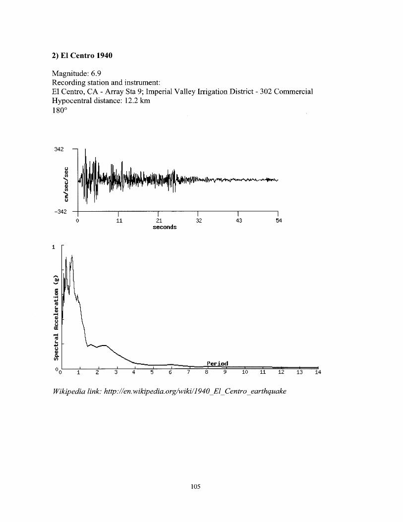
2) El Centro 1940
Magnitude: 6.9Recording station and instrument:El Centro, CA - Array Sta 9; Imperial Valley Irrigation District - 302 CommercialHypocentral distance: 12.2 km1800
342
C
-342-
0 11 21 32 43 54seconds
I
L
4j
C)
0 ' ' ' ' 'Perioi0 1 2 3 4 5 6 7 8 9 10 11 12 13 14
Wikipedia link: http://en.wikipedia.org/wiki/1940_ElCentro-earthquake
105

3) Kern County 1952
Magnitude: 7.5Recording station and instrument:Taft, CA - Lincoln School - 810 N SixthClosest distance to fault: 36.2 km210
150
-1500 11 22 33 43
seconds
1P
.0
L.
54
Period0 1 2 3 4 5 6 7 8 9 10 11 12 13 14
Wikipedia link: http://en.wikipedia.org/wiki/1952_Kern_Countyearthquake
106

4) San Fernando 1971
Magnitude: 6.6Recording station and instrument:Pacoima Dam, CAClosest distance to fault: 3.5 km1640
1148
-1148
0 4 8 12 16 20seconds
3
W
L
Period
0 1 2 3 4 5 6 7 8 9 10 11 12 13 14
Wikipedia link. http://en.wikipedia.org/wiki/]971_SanFernando-earthquake
107

5) Imperial Valley 1979
Magnitude: 6.6Recording station and instrument:Bonds Corner, CA - Omlim residence - Hwys 115 & 98Closest distance to fault: 4.4 km1400
576
-576 |
0 8 15 23 30 38seconds
2
CL
Period
01
0o 1' 2' 3' 4' 6 7 8 9 10 11 1'2 13
Wikipedia link: http://en.wikipedia.org/wiki/List of earthquakes inCalifornia
108

6) Livermore A 1980
Magnitude: 5.9Recording station and instrument:San Ramon, CA - Fire StationHypocentral distance: 19.5 km3400
0 8 16 24 32seconds
I-
I
Wikipedia link: http://en.wikipedia.org/wiki/List of earthquakesinCaliornia
109
38
-38
1~
0r
40
2Per
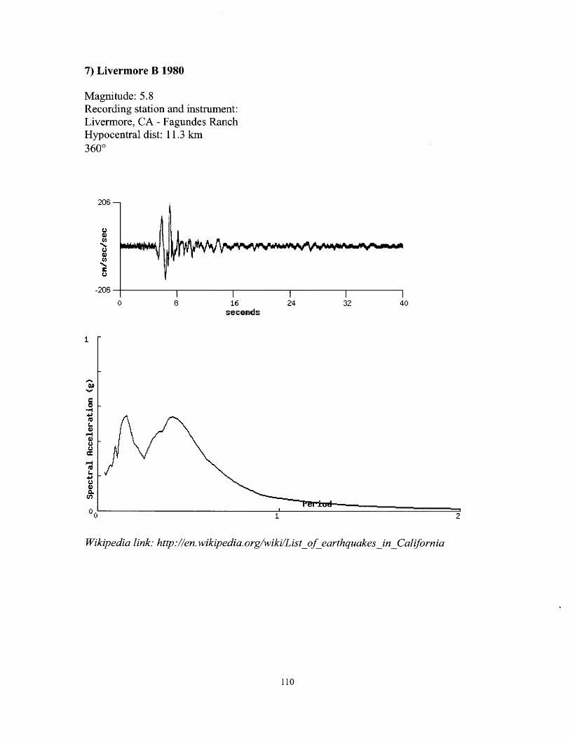
7) Livermore B 1980
Magnitude: 5.8Recording station and instrument:Livermore, CA - Fagundes RanchHypocentral dist: 11.3 km3600
206-
-206
0 8 16 24 32 40seconds
0
1 -
0
P-
002
00 1' 2
Wikipedia link: ht'tp:/en. wikipedia. org/wiki/ListofearthquakesinCalfornia
110

8) Coalinga 1980
Magnitude: 6.5Recording station and instrument:Pleasant Valley, CA - Pumping PlantHypocentral dist: 14.1 km450
307
C0
-307
0 12 23 35 46seconds
P~eriod __
1 2 3 4 5 6 7 8 9 10 11 12 13 14
Wikipedia link. http://en.wikipedia.org/wiki/]983_Coalingaearthquake
111
58
2
0
C-Cn:
~
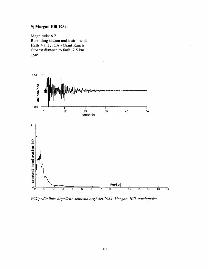
9) Morgan Hill 1984
Magnitude: 6.2Recording station and instrument:Halls Valley, CA - Grant RanchClosest distance to fault: 2.5 km1500
153
-153
0 12 24 36 48seconds
1
0
Period1 2 3 4 5 6 7 8 9 10 11 12 13 14
Wikipedia link. http://en.wikipedia.org/wiki/1984_MorganHill-earthquake
112
60

10) Whittier 1987
Magnitude: 6.1Recording station and instrument:Monterey Park, CA - Garvey ReservoirClosest distance to fault: 13.6 km3300
468 -
-468 I I0 5 11 16 22
seconds
2
CL
0.
Period
113
0 1 2 3 4 5 6 7 8 9 10 11 12 13 14
Wikipedia link: http://en.wikipedia.org/wiki/1987_WhittierNarrows-earthquake

11) Loma Prieta 1989
Magnitude: 7.0Recording station and instrument:Corralitos, CAClosest distance to fault: 2.8 km00
618
-618
0 8 16 24 32seconds
3
0
L
40
reriodI 2 3 4 5 6 7 8 9 10 11 12 13
Wikipedia link: http://en.wikipedia.org/wiki/1989_LomaPrieta-earthquake
114

12) Sierra Madre 1991
Magnitude: 5.8Recording station and instrument:Sierra Madre, CA - Cogswell Dam (Ctr Crest)Hypocentral distance: 12.6 km1550
477 -
IU
-477
0 8 16 24 32 40seconds
2
W
Wikipedia link: http://en.wikipedia.org/wiki/List of earthquakes_inCal fornia
115

13) Petrolia 1992
Magnitude: 7.1Recording station and instrument:Cape Mendocino, CA - PetroliaHypocentral distance: 15.5 km00
1468
-1468
Wi! I ~F~- --- ~Ut~
rITTvv
0
4
.0
P-
0
12
Period1 -2 3 4 5 6 7 8 9 :10 11 12 13 :14
Wikipedia link: http://en.wikipedia.org/wiki/l992_CapeMendocinoearthquakes
116
24seconds
36 48
-- w

14) Landers 1992
Magnitude: 7.3Recording station and instrument:Joshua Tree, CA - Fire StationClosest distance to fault: 10.0 km00
268
-268 | |
0 16 32se
I
.P4
L
to
48 64conds
Period
2 3 4
Wikipedia link: http://en.wikipedia.org/wiki/]992_Landersearthquake
117

15) Big Bear 1992
Magnitude: 6.5Recording station andSnow Creek, CA
instrument:
Hypocentral distance: 37.9 km1800
117
-117
0
I
12
0A
4j
eL
Period5
Wikipedia link: http://en.wikipedia.org/wiki/1992_BigBear earthquake
118
24seconds
36 48
I I '
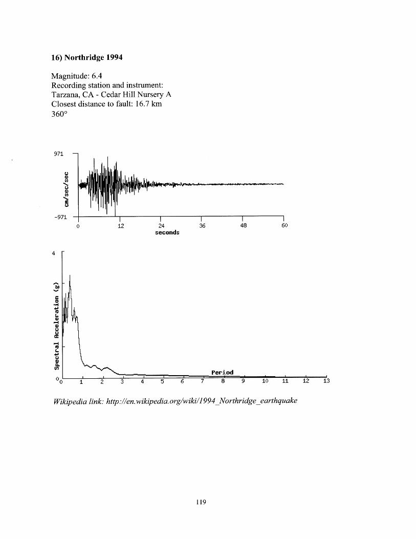
16) Northridge 1994
Magnitude: 6.4Recording station and instrument:Tarzana, CA - Cedar Hill Nursery AClosest distance to fault: 16.7 km3600
971
-971 -T
0 12 24secon
4
.C24
P-aD
P-
00 1 1 1 1 3 4 1 5
36 48ds
Period
Wikipedia link: http://en.wikipedia.org/wiki/]994_Northridgeearthquake
119
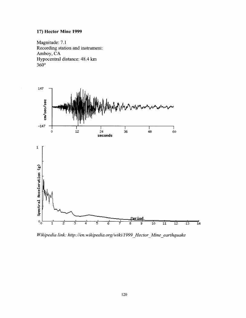
17) Hector Mine 1999
Magnitude: 7.1Recording station and instrument:Amboy, CAHypocentral distance: 48.4 km3600
147
z,U
-147
0 12
C
0
L
0 1 2 3 4 5 6 7 8 9 10 11 12 13 14
Wikipedia link: http://en.wikipedia.org/wiki/1999_HectorMine-earthquake
~Yw~Aw
24seconds
36 48 60
3rio(I
120
I IIJ, I I,,
.11
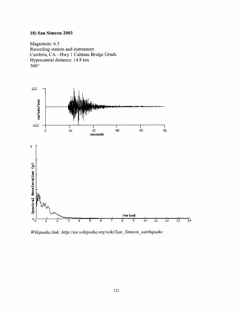
18) San Simeon 2003
Magnitude: 6.5Recording station andCambria, CA - Hwy 1Hypocentral distance:3600
122
-122
instrument:Caltrans Bridge Grnds14.8 km
i i I1.
0 16 32 48 65seconds
81
________________Period
1 2 3 4 5 6 7 8 9 10 1i 12 13 14
Wikipedia link: http://en.wikipedia.org/wiki/SanSimeonearthquake
121
1
p4
P-
-1-
0L
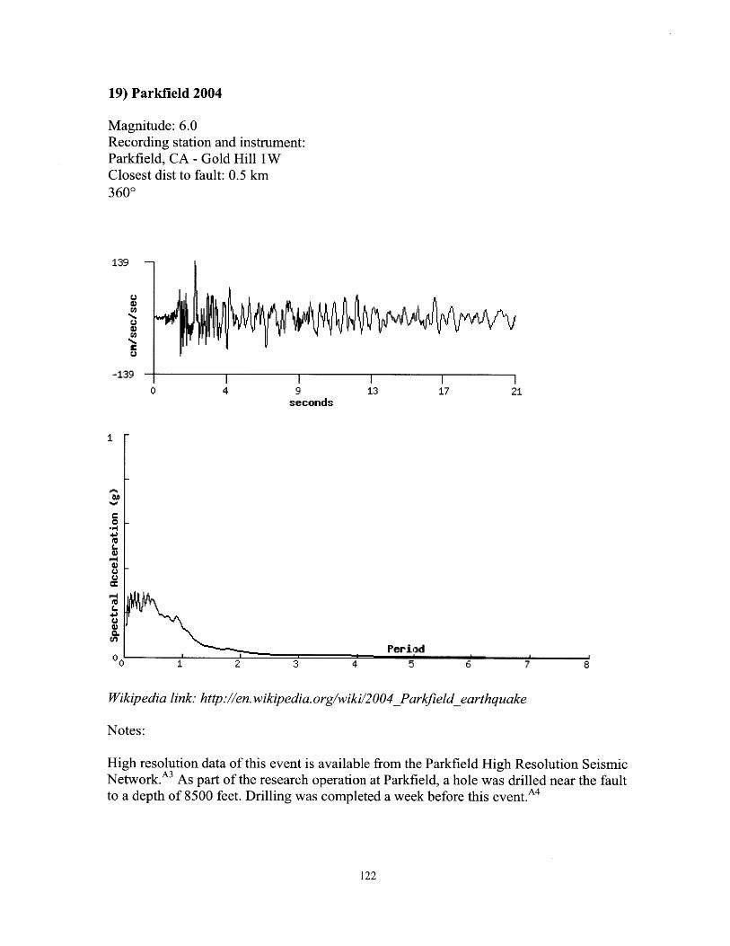
19) Parkfield 2004
Magnitude: 6.0Recording station and instrument:Parkfield, CA - Gold Hill 1WClosest dist to fault: 0.5 km3600
139
C
-139
0 4 9 13 17 21seconds
I
.4
10
P-1
01.
0'SPerid
7 81 2 3 4 5 6
Wikipedia link. http://en.wikipedia.org/wiki/2004_Parkfield earthquake
Notes:
High resolution data of this event is available from the Parkfield High Resolution SeismicNetwork.A3 As part of the research operation at Parkfield, a hole was drilled near the faultto a depth of 8500 feet. Drilling was completed a week before this event.A4
122
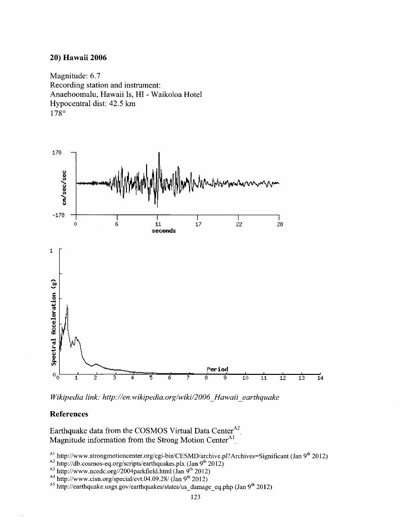
20) Hawaii 2006
Magnitude: 6.7Recording station and instrument:Anaehoomalu, Hawaii Is, HI - Waikoloa HotelHypocentral dist: 42.5 km1780
178
C7
-178
0 6 11 17 22seconds
28
________Period
1 2 3 4 5 6 7 8 9 10 11 12 13 14
Wikipedia link: http://en.wikipedia.org/wiki/2006_Hawaiiearthquake
References
Earthquake data from the COSMOS Virtual Data CenterAMagnitude information from the Strong Motion Center Al
Al http://www.strongmotioncenter.org/cgi-bin/CESMD/archive.pl?Archives=Significant (Jan 9 th 2012)A2 http://db.cosmos-eq.org/scripts/earthquakes.plx (Jan 9 th 2012)A3 http://www.ncedc.org//2004parkfield.html (Jan 9 th 2012)A4 http://www.cisn.org/special/evt.04.09.28/ (Jan 9 th 2012)A5 http://earthquake.usgs.gov/earthquakes/states/us_damage-eq.php (Jan 9 th 2012)
123
I
0.3-I.IJ
I-Ia,C.,C.,
C-
a,0.
00


Appendix B: A Set of Benchmark Building Models for Usein Simulations
B.1. Index of Symbols Used
Symbols are defined as they are used, and are also defined here for reference.
A constant used to simplify the calculation of parabolic stiffness distribution. Defined in eqn B.53
CT variable used by the ASCE 7-05 code to find the approximate first natural period
D the fractional increase in stiffness, of k1, that defines a linearly-increasing stiffness distribution
d The linear increment of lower story stiffnesses as a fraction of k1. Defined in eqn B. 11
story drift
E material stiffness modulus
e rigid body vector. Defined in eqn B.9
F, force on structure node i. In particular the forces in the wall-building links
F vector of forces Fi
Fw. vector of the net loads on the wall
vector of the net loads on the wall but incomplete as FN = 0
Fb vector of the net loads on the building
Fwall wall pseudo-flexibility matrix, determining shape from loads
F1 a 'flip' matrix. Defined in eqn B.28
H total height of the building
h, h, single story height
h, the height of the it, jTh story
I the identity matrix
second moment of area, usually of the rocking wall
the rotational moment of inertia of the rocking wall
the story stiffness of the it' story, where i= 1 is the top story
k story stiffness. If no subscript, then represents constant story stiffness
k stiffness vector of the building story stiffnesses
K stiffness matrix, either of the building, or of the whole building-rocking wall system ,depending on context
Kwaii wall pseudo-stiffness matrix, determining loads from shape
Kbld the stiffness matrix of the building
L a lower triangular matrix where the lower triangular elements are all unity. Defined in eqn B. 16
L length, either of a single story, or the total height of the rocking wall, depending on context
M diagonal matrix of the masses in a building. Defined for the standard top-light case in eqn B.3
M total mass of the rocking wall
m mass of any non-top story, when using the standard top-light mass distribution
mi the mass of the ith story
N the number of stories in the building
Pj load on building position i
P vector of Pi
Qj load on wall position i
125

Q vector of Qi
SD/L a matrix that shifts elements down or left depending whether it pre- or post-multiplies. Defined in eqn B.5
SUR a matrix that shifts elements up or right depending whether it pre- or post-multiplies. Defined in eqn B.6
Ss Igeographical short period acceleration
T, T1 first natural period, usually of the building
Ta approximate first natural period
ut displacement of building node i
U vector of uj
U an upper triangular matrix where the upper triangular elements are all unity. Defined in eqn B. 17
vi displacement of wall node i
V vector of vi
v linear vector which is the standard initial guess for the building first mode.
V the base shear in an equivalent seismic load calculation
V diag(v), a diagonal matrix of the linear vector v. Defined in eqn B.58
W shape displacement vector for wall, as measured from some rotational datum line
Wi ith element of W
On, 01 first natural angular frequency, usually of the building
V angle through which the datum line (projected through the hinge and position N) of the wall has rotated
vector representing a rigid body rotation of y
B.2. Conventions
In this appendix, the top node of a discretized building is referred to as node 1, while the
lowest node is referred to as node N. This is in contrast to the work body.
126

B.3. Introduction
In order to present details of the most useful rocking wall size for representative building
types, those representative buildings must first be defined.
There are many ways in which this could be done. The method that seems most natural is
to start with basic assumptions that a structural engineer would have about a building of a
given size. One of the earliest appreciations that an engineer has is of the natural period
of a building.
The natural period may be estimated with the familiar T ~~0. IN. However, that is a very
rough approximation, and can be considerably off, especially for certain kinds of
structure. A better approach to approximate the period is to follow the guidelines in a
widely accepted code, such as ASCE 7-05. ASCE 7-05 considers almost all building types
when calculating the natural period, and although it usually produces a result within 25%
of T ~~0. IN, is not constrained by the assumptions in that formula.
In addition to story masses, the only other piece of information needed to determine the
story stiffnesses is the stiffness form. For example, it is required to know whether the
story stiffnesses are uniform, or increase linearly from the top down, or increase
parabolically from the top down. It is not possible to model every building, but rather a
representative set of models may be determined, one of which will offer a reasonable
approximation to most given rocking wall installations, and thus provide data which
simplifies the analysis process.
127

It is important to understand that if, in addition to the mass distribution, the stiffness form
(constant/linear/parabolic) is known, and code is used to determine the natural period,
then the code fully implies the stiffness matrix. Developing a stiffness matrix in addition
to using code to determine the natural period is redundant. Likewise, if the stiffness
matrix is known, then using the code to find the period is redundant. And since code
provides a very useful approximation of the natural period of buildings, it may also be
extended to provide a useful set of representative building models. Making the leap from
natural period to stiffness matrix, given the stiffness form, requires some careful algebra,
which is presented here.
Based on the mass, mass form, and stiffness form, algebra may be applied that rearranges
the Rayleigh quotient formula, including inverse iteration, to provide the building
stiffnesses, to determine the story stiffnesses, and thus produce a set of representative
discretized building models. An example will also be used to suggest that using five
inverse iterations is equivalent for any reasonable purpose to a closed-form solution.
In the case where the story stiffnesses are uniform, the Rayleigh quotient is not required,
since the closed-form solution may be applied:
co2 = 4!sin (Bm 4N
where N is the number of stories, m is the story mass of a standard top-light building
model, and k is the story stiffness.
128
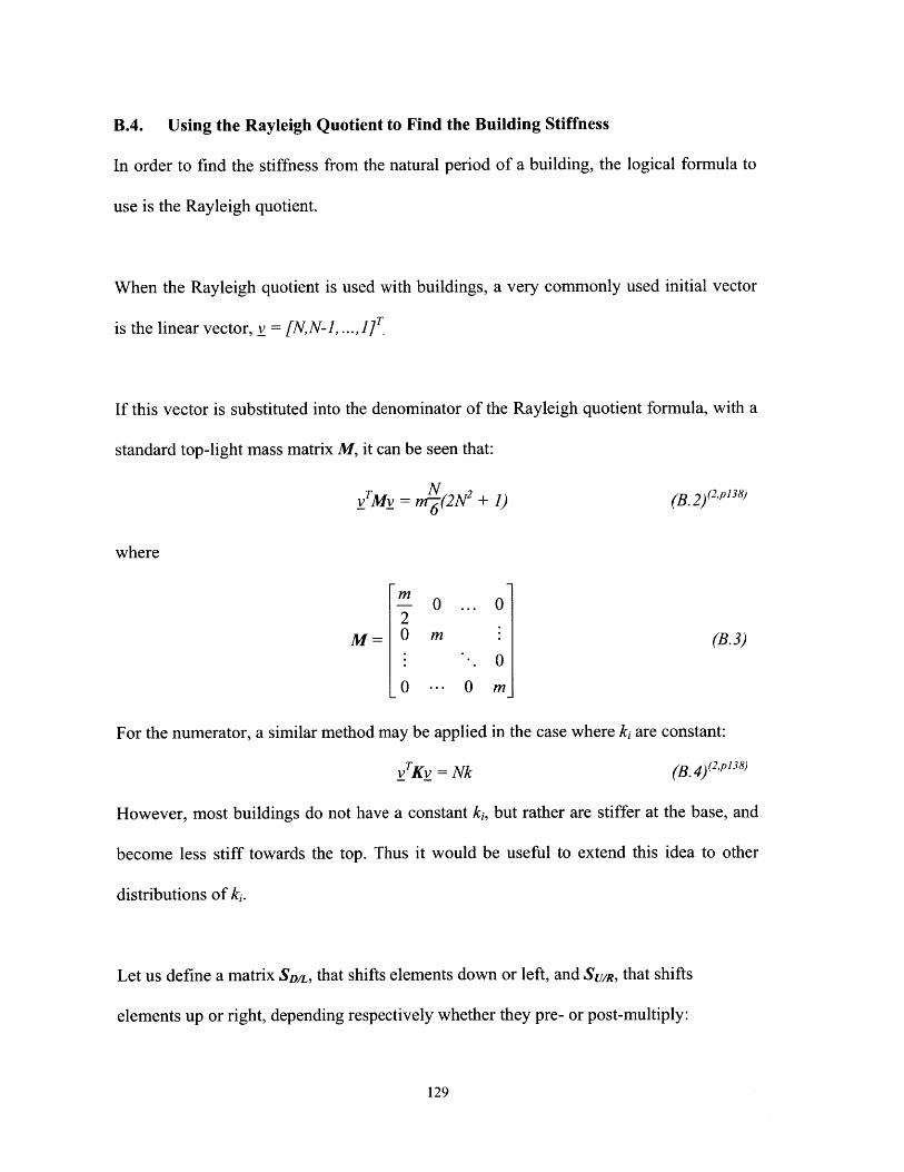
B.4. Using the Rayleigh Quotient to Find the Building Stiffness
In order to find the stiffness from the natural period of a building, the logical formula to
use is the Rayleigh quotient.
When the Rayleigh quotient is used with buildings, a very commonly used initial vector
is the linear vector, v = [N,N-1,...,1]
If this vector is substituted into the denominator of the Rayleigh quotient formula, with a
standard top-light mass matrix M, it can be seen that:
vTMv = nr (2N2 + 1) (B.2)(2P]8
where
- 0 ... 02
M= 0 m (B.3)* .0
0 --- 0 M_
For the numerator, a similar method may be applied in the case where ki are constant:
y Kv = Nk (B.4)2,8
However, most buildings do not have a constant ki, but rather are stiffer at the base, and
become less stiff towards the top. Thus it would be useful to extend this idea to other
distributions of k;.
Let us define a matrix SD/L, that shifts elements down or left, and Su , that shifts
elements up or right, depending respectively whether they pre- or post-multiply:
129
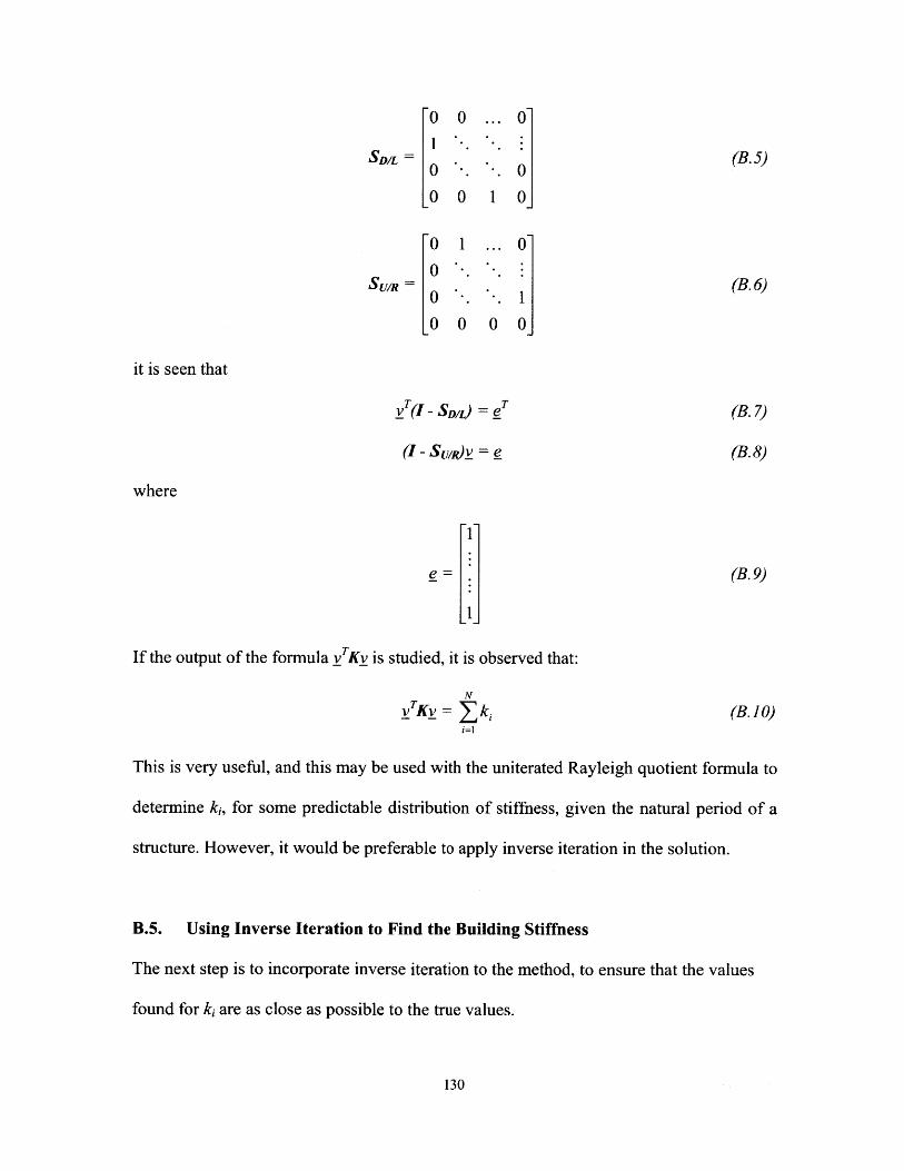
0 0 ... 0
SD/L = (B.5)0 - -. 0
0O 0 1 01
0 1 ... 0
SUIR = . . (B. 6)
0O 0 0 0j
it is seen that
v(I - SDI) =eT (B. 7)
(I - SumR)v = e (B.8)
where
e = . (B.9)
If the output of the formula vTKv is studied, it is observed that:
NvKv = ki (B. 10)
i=1
This is very useful, and this may be used with the uniterated Rayleigh quotient formula to
determine ki, for some predictable distribution of stiffness, given the natural period of a
structure. However, it would be preferable to apply inverse iteration in the solution.
B.5. Using Inverse Iteration to Find the Building Stiffness
The next step is to incorporate inverse iteration to the method, to ensure that the values
found for k; are as close as possible to the true values.
130

However, the Rayleigh quotient formula only allows us to solve for one variable, so in
order to use inverse iteration, a stiffness matrix must be formulated specifically for a
given arrangement of stiffnesses, in terms of a fixed variable that defines the stiffness
distribution, such as k;.
When each story stiffness is a successive multiple of the top stiffness (i.e. in the
following example, the increment d=]), the structure deforms linearly, under uniform
loading.3'' 58 Let us consider the general linearly-increasing case, in which the increment d
may be less than or greater than unity:
ki = k; + (j-1)dki (1 j < N; d e -i) (B.11)
It is required to solve the following for ki, or some other variable that uniquely specifies
the stiffness matrix, given the stiffness arrangement:
v'ET((K- M)T)" K (K -M) " v(B2vT ((K M)T)n M(K -'M)"v
Since it is known that:
vT Kv = k (B.13)
and by definition:
N
elk = ki (B. 14)
it may be equated in the general case:
ek =Kv (B.15)
131

It would be helpful if k, a vector of story stiffnesses could be solved for, knowing K.
Define:
L = K
0U =
0
L0
0 ... 0~
I .U.- 1 1
(B.16)
(B.17)
and thus:
v Ue
T TV AL
(B. 18)
(B. 19)
Also note that:
(I - SD/L) L^
(I - SUIR) = U~
Thus equation B. 19 may be rearranged for eT, and substitute into equation B. 15:
(I- SDRL)k vTKv
And so the following may be observed in the general case:
k = LKv
LKU = diag()
k = LKUe
Thus, to find K as a multiple of k1, or of some other variable that defines a specific
(B. 10)
(B. 21)
(B. 22)
(B.23)
(B.24)
(B.25)
arrangement of stiffnesses, first diag(L must be defined as a multiple of that variable.
132
B.5.1. Linear Stiffness
For the linear case,
k = k;
I
1+d
1+ 2d
1+ (N - I)d
diag(k) = k;(I + dSD/LFVFSu/R)
where F, is a 'flip' matrix:
0
F1=0
LI
-- 0 1
.' 0
0 --- 0
where it might be noted that U = FILF. V is the linear diagonal matrix:
-N
T 0V = diag(v) = ye .*I =.
: 0
0 --- 0o ]N-i
0 0
-- 0 1
thus substituting equation B.27 into equation B.24,
ki(I + dSD/LFjVFSup) = LKU
rearranging:
and so
K = k1(I - SD/L)(I + dSD/LFiVFPS/)(I - SuR)
1K' = TU(I + dSD/LFIVFISU)~' L
133
so
(B.26)
(B.27)
(B.28)
(B.29)
(B.30)
(B.31)
(B.32)
This linearly increasing K may thus also be substituted into the uniterated Rayleigh
quotient formula as a simple multiple of k1 :
vTKv = kivT(I - SD4)( I + dSD/LFiVFISu/P)(I - SuR)v (B.33)
simplifying:
Kv = ek = kjfT(I + dSDIjFVFSVUI)e (B.34)
The mass matrix may also be defined in terms of such standard matrices, multiplied by a
constant:
M - 2 ±( +SDILSU/R) (B.35)
and so:
KIM = + dSD/LFVFS1)-'L(I + SD/LSU/R) (B.36)
Thus, in the linear case, the nth iteration of the first eigenvector is:
= (K'M) v =2k[U(I + dSD/LFVFASU/)~'L(I + SD/ )]nv (B.37)
where high n may simply be chosen to very closely approximate the true eigenvector.
The constants may be neglected of course. Thus the iterated Rayleigh quotient formula
for k, may be evaluated:
co v Mvki -vn Kv,,
ki
co1 2vT(I+SD/LSUIR)Vn
r (2vn (I - SDI L)(I +dSDI LF VFSU1I R SUI R)n
(B.38)
(B.39)
which may be found in non-dimensional form:
134
kinMi CO
Iv;T(I + SD/ LSUI R)vn2y
,_V 1- SDL)(1 +dDLF VFISUIR)(1 - U/RV,
(B.40)
where v, is found in equation B. 37. The constants multiplying v and v' are not required.
B.5.2. Constant Stiffness
Now that the case of linearly increasing story stiffnesses has illuminated the issues, let
the simpler case be considered, where ki are constant.
Equation B.1 may be rearranged to find k in the constant case, or d=O may be set in
equation B.40. But let the problem also be solved from scratch, in order to compare the
results.
For the constant case,
diag(k) = kI
substituting into equation B.24:
rearranging:
kI = LKU
(B.41)
(B.42)
(B.43)K = k(I - SD/L)(I - SU/R)
and so
K1
Then if the mass matrix defined in equation B.35 is multiplied by, then:
K'M = U L(I + SD/LSU/R)
(B.44)
(B.45)
135

Thus, in the constant case, the n'h iteration of the first eigenvector is:
n= (K'M)" v = j[ UL(I + SD/LSU,/R))]n v (B.46)
where again high n may simply be chosen to very closely approximate the true
eigenvector, and neglect the constants. Thus the iterated Rayleigh quotient formula for k
may be evaluated:
k =- -2ET(B.47)v TKv
k
co v (+SDILSUIR)
= 2 (B.48)v (I -SDL )(I-SUIR(B8
which matches equation B.40 where d = 0. v=v may be substituted from equation B.46.
The constants multiplying v and v' are not required.
The performance of this formula is excellent as expected. It may be compared with the
closed-form solution non-dimensionally:
N2 cosec2N (B.49)2 ,P13 9 )
For N = 10, the closed-form solution yields 40.611909699 to 9 d.p. Equation B.48 yields:
Iterations mwo2 Error (%)k
0 33.5 17.511 40.556 1.4x10-'2 40.61124 1.6x10 3
3 40.611901 2.1x10⁻⁵
4 40.6119096 2.7x10⁻⁷
5 40.611909698 3.4x10⁻⁹
Table BL. The output of equation B.48 compared with the closed-form eigenvalue formula
136
As can be seen from table B1, with each iteration, the error is about two orders of
magnitude better. It seems clear that using five iterations would ensure an entirely
negligible difference between the estimated value and the true value. The software
developed in this work uses 50 iterations, which is computationally trivial.
B.5.3. Parabolic Stiffness
Since seismic loading is parabolic in nature, a common strategy in building design is to
have the stiffness form be parabolic.
It can be seen that if constant story drifts 5 are required to ensure that damage is spread
evenly, then:
kI=-FUR (B.50)
where k is the stiffness vector, and p is any load vector. The inspiration for this neat
formula (equation B.50) is Jerome Connor's Introduction to Structural Motion Control,
which gives a more general form for any desired drift arrangement' 58 . It so happens that
for constant story drifts, the stiffness vector k may be expressed in terms of the standard
matrices previously defined.
For equivalent seismic loading, that the loads p; may be defined as:
j Zhi m,
137
(B. 51) (4p 1 0

in which k = 2 unless the period is less than 0.5s, in which case k = 1, with the option for
linear interpolation between 1 and 2 if the natural period is between 0.5s and 2.5s. For the
case k = 2, and for the standard top-light mass model, this can be expressed in vector
form as:
2p = Vm h 0
him -0
L0
0
1 .. (B.52)
where hs is the single story height. Denote the constant:
Vm h2 =A
Z him,(B. 53)
1p = 2A(I+ SD/LSU/R)
N 2
N 2 -2N+1 2
N 2 -4N+2 2
_N2 -2(N -1)N +(N -1) 2
I=A 2(I + SD/LSU/R)[N22 -
0
2
4
_2(N -1).
0
12
2 2
_(N -1) 2
1=A(I + SD/LSU/R)[N 2 e - 2NSD/LFIUe + F(SU/RVSD/L) 2e]
1= A(I+ SDILSU/R)[N 2 - 2NSD/LFIU + FI(SU/R VSD/L2]e
138
then:
(B.54)
I (B.55)
(B.56)
(B.57)

where V = diag(v):
N 0 ... 0
0 N-1:V= . (B.58)
: -. 0
L0 --- 0 1
And thus substituting equation B.57 into equation B.50:
Ak -2 FU(I + SD/LSu/)[N 2I - 2NSD/LFlU + F(Sum VSD/L)2]e (B. 59)
215
And thus from equation B.24:
LKU = diag@ (B. 60)
It is possible to determine diag() in the parabolic case directly in terms of standard
matrices, but the formula is very long, and there is no real benefit to it. Rearranging:
K = (I - SD/L)diag()(I - SU/p) (B.61)
and thus:
K' = U[diag(@)]-'L (B. 62)
Then if the mass matrix defined in equation B.35 is multiplied by, then
K'M = IU[diag(k)]-iL (I + SD/LSU ) (B. 63)
Thus, in the parabolic case, the n' iteration of the first eigenvector is:
v= (K'M
m"
~ 2 [U[diag(k]-'L (I + SD/LSU V v (B. 64)
where high n may simply be chosen to very closely approximate the true eigenvector,
with the constants neglected. Thus the iterated Rayleigh quotient formula may be
evaluated, in this case solving for 5, the constant interstory drift:
139

t v KvW 2 T
>5v Mv
SvT(I - SD/L)diag (I - SUq)v(B. 65)
2o ±(I + SD/LSU/Rv
v=v may be substituted from equation B.64. The constants multiplying vn and y' are
again not required. Taking (5 to the outside of diag@, t may now be substituted into
equation B. 61 to obtain the stiffness matrix.
In summation, the stiffness vector, matrix and mode may be found in any of the three
cases with inputs N, w1 , and m, with the addition of d in the linearly increasing case.
An alternative use for equation B. 65 is to specify the desired story drift 5 for a parabolic
stiffness arrangement, which will provide constant story drift under equivalent seismic
loading, and solve for the resulting period and hence stiffnesses. The same is true for any
of the previous stiffness arrangements.
140

B.6. Representative Model Building Data with Rocking Wall Design Data
56 representative model buildings are presented, with 116 rocking wall configurations,each with a graph of maximum storey drift vs. rocking wall size.
The storey drifts were determined using the static equivalent seismic loading method, andwere based on a location of Los Angeles, California. The story stiffnesses weredetermined by extrapolation from the code-derived period and the mass of each structure.The constant data used to determine the period of the buildings and seismic loads fromASCE 7-05 were:
Story Height 3.3mOccupancy Category 3 (e.g > 300 people)
1-second Spectral Acceleration S, 0.75Short-period Spectral Acceleration Ss 1.5
Site Class DLLRS Concrete Moment Frame
Response Modification Factor R 4
Long Period Transition Period TL 8
Other constant data were:
Rocking Wall Depth 0.61m
Average Density 400 kg/m3
The data modified for each model building were:
N Number of stories
Height:width Ratio 2 to 5 stories: 16 to 10 stories: 211 to 15 stories: 3(square plan)
m The single story mass m based on theabove.
Stiffness Form (d) Four different linear stifnessjbrmswere tested, with d (the increase instiffness of lower stories as afraction ofthe upper storey) as 0.0, 0.25, 0.5, and1.0. Thus only the top story stiffness ,topis given in the tables. The otherstiffnesses can be inferredfrom ktrop andd
Number of Rocking Walls 2-5 stories: one pair of rocking walls,6-10 stories: up to two pairs,15 stories: up to three pairs.
Each graph has been cropped to show only the most relevant data. It may be noted thatthe small stiff buildings of 2-4 stories have very low story drifts, but from 5 to 15 stories,all of the data are in the 0.4-0.7% range, and produce some very interesting andsometimes unexpected graphs, which may be confirmed in any finite element softwarepackage.
141
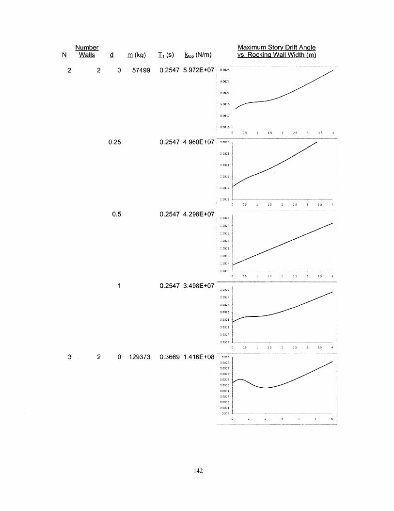
Number Maximum Story Drift AngleN Walls d m (kg) I (s) htop (N/m) vs. Rocking Wall Width (m)
2 2 0 57499 0.2547 5.972E+07 a0025
00023
0 001;
0 0015
3 (.5 1 15 2 23 3 3, 4
0.25 0.2547 4.960E+07 0025
D 0023
3 0021
3 0019
0 00171
3,0015
5 3 1 13 2 25 3 3.5 4
0.5 0.2547 4.298E+07
3 002-7
0 0021
32315 - - -- - - - - - -
5 1 15 2 2. 35 4
0.2547 3.498E+07 0 0029
0 0027
30023
3 0017*
S 3,5 1 15 2 25 3 35 4
3 2 0 129373 0.3669 1.416E+08 ns3 0029 10,00270,0026
0,0023
0021
0 00 2 - - - - - - - - - - - -
2 3 4 5 6
142

NumberN Walls d m (kg) l (s) htop (N/m)
Maximum Story Drift Anglevs. Rocking Wall Width (m)
0.3669 1.030E+08
0.3669 8.237E+07
0.3669 6.043E+07
3 303
0 002950 0029
0 00285
0 0328;
3002657
3 00295
0 00265
3,33355
3 002
3 3339
03333
3 03-75
3 3023
3 05 1 ~ 15 2 25 3
3 05 1 15 2 -5
0 0035
0,0033
3 315
0 00313 15
3 0303
333293
5 6 7 S
0.4754 1.715E+08 0003,
3 0033
3 3333
0 0032
3 00315
143
0.25
3 30297
3 3026
333
03.
0.5
1
4 2 0 229997 0.4754 2.639E+08
0.25
,,,ooooooooo-

NumberN Walls d m (kg) L (s) jtop (N/m)
Maximum Story Drift Anglevs. Rockina Wall Width (m)
0.4754 1.296E+08 00035
3,00345
3 0034
300335
0 0033
2 0 359370 0.5811 4.292E+08
300375
0037
3 00365
0 0033
300355
0 0033
33034 -0003
3 0033
3 33356
33334 4-
00040s
300395
o 0039
000385
0 00375
373o37 -
300415
00041o c35
3 39
3385
3 4 57
144
0.5
1 0.4754 8.928E+07
5
0.25
0.5
0.5811 2.523E+08
0.5811 1.828E+08
5 6 7
-L
1
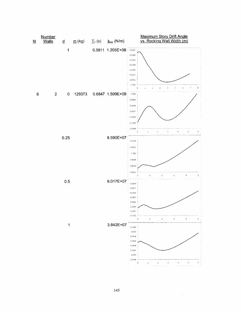
NumberN Walls d m (kg) l (s) op (N/m)
Maximum Story Drift Anglevs. Rockina Wall Width (m)
1 0.5811 1.205E+08
2 0 129373 0.6847 1.599E+08
0.25 8.590E+07
0.5
1
6.017E+07
3.842E+07
03047
0 0046
o 0045
0 0044
30043
O 5344
305
0 0049
0 004FS
1 - 3 4 5 6
3 '540 034355544
3 1 4 50 00550.03343
30034
0 0051
5 1 2 4
3 0049
3L47
330045 ----
3 00542
3 005
003
S 1 2 3 4 5 6
145
6
D 4

NumberN Walls d m (kg) l (s) htop (N/m)
Maximum Story Drift Anglevs. Rockina Wall Width (m)
4 0 129373 0.6847 1.599E+08
0.25 8.590E+07
0.5 6.017E+07
3337
0 0065
0 0055
30 004 53
0 1 2 3 4 5 6
30065
333055
3 33
00045
0314
3,307
336
S0055
333045 -
0 0068
0.0068
0,0054
1 23 4
3 0367
0.0055
33054
0 0052
3 3 4
0.0055
0 0051
0 005
0 0049
0 0049
1 3.842E+07
2 0 176091 0.7866 2.241E+08
3 0047-r - - - -3
146
7
3 4
13

d m (kg) I (s) stop (N/m)
0.25
0.5
1
1.109E+08
7.561 E+07
4.709E+07
4 0 176091 0.7866 2.241E+08
0 0059
0 0057
3 0055
0 0053
0 005 1
3 0049
0 0047
30045
00064
0 0052
0 336
0 0064
3 0336
33 335
3 3368
0,3366
D 0364
3 0356
D 3 4
00307
NumberN Walls
33363
336
3 333~
3 333
13
1.109E+080007~
33306
03'30 1
3330-5
3304,
147
Maximum Story Drift Anglevs. Rocking Wall Width (m)
---------------
-4 -
34 6 8
10
1D
10
0.25

NumberN Walls d m (kg) I (s) ktop (N/m)
0.5 7.561 E+07
Maximum Story Drift Anglevs. Rocking Wall Width (m)
3003
0075
333065
0306
2 4 6 8
4.709E+07
0007
3 3365
2 0 229997 0.8871 3.003E+08
3349
3 30445
33347
3) 3475
5 2
1.379E+08 3336
3 0054
9.189E+07 7336
3 3059
3 0058
30057
3,005530054
0 0053
0 0052
0.3os3305
3 2 4 6 8
1
10
8
0.25
0.5
13
13
148
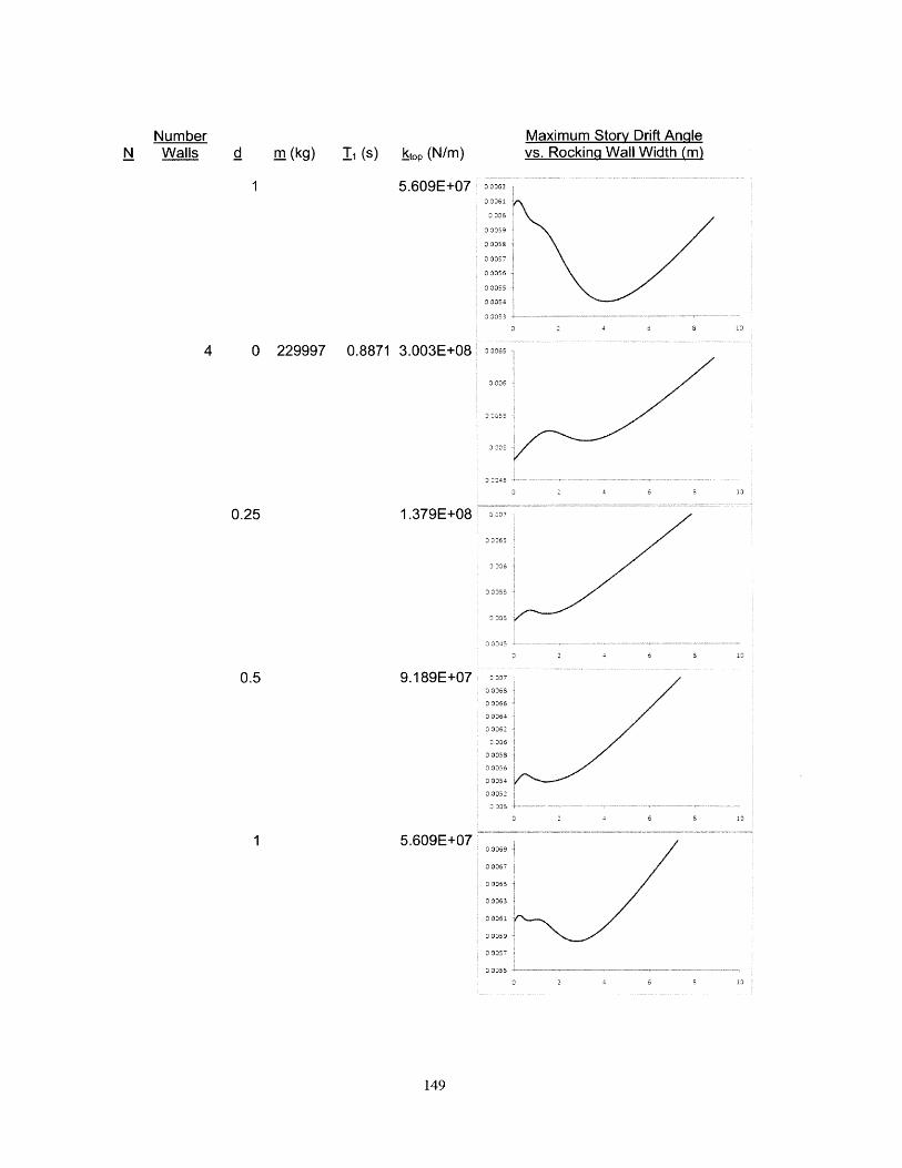
Number Maximum Story Drift AngleN Walls d m (kg) li(s) op (N/m) vs. Rocking Wall Width (m)
1 5.609E+07 000620 3061
0 0053
0 0.055
3 0054
3 - 4 5 13
4 0 229997 0.8871 3.003E+08 0065
000645D 0 4 S 13
0.25 1.379E+08
D 3345
3 0044
0.5 9.189E+07
0 01054
00052
0 005 -
3 00633 3016
3 0061
30054
00052
3 3 5 --- - - - - - - - - - - - ,
3 2 4 6 S 13
5.609E+07
00065
o m iJ 33 1
3 3351
30319
3 33~6
149
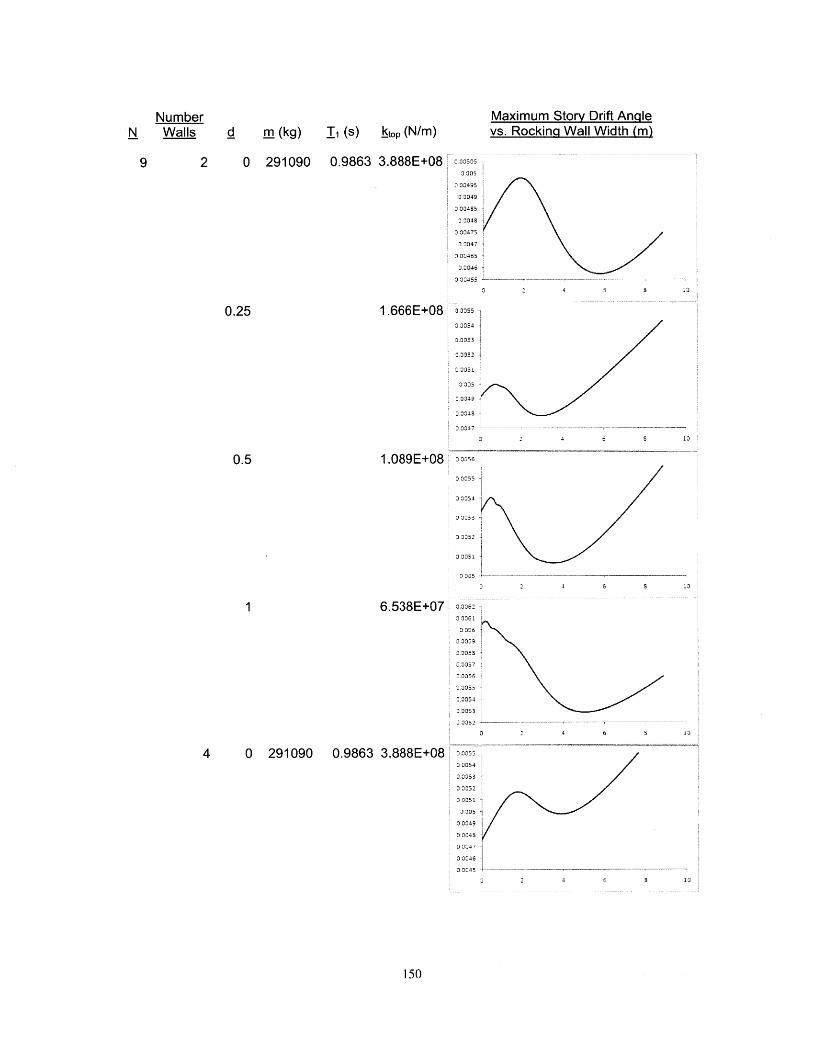
NumberN Walls d m (kg) l (s) ktop (N/m)
Maximum Story Drift Anglevs. Rocking Wall Width (m)
2 0 291090 0.9863 3.888E+08
1.666E+08
30535
3 349
0.00485004
0004750 0047
1.00465
0.0046330455
0 0055
0 0054
3 3053
3 0052
0 005
0 04 9
0 0047 --
6 8
6
1.089E+08 30356
0 355
3 0054
3 3353
3 3351
3335
6.538E+073061
33355
0 0058
00057000563 3355
0 0054
3.0053
3 0052
4 6
4 0 291090 0.9863 3.888E+08 333550,0054
00053
D 0052
0 0051
0 0049-
0.004S
3 0046
3 0045 -
2 4 6
150
9
0.25
0.5
10
1
53
-- - - - ^
4 6

NumberN Walls d m (kg) _i (s) htop (N/m)
0.25 1.666E+08
Maximum Story Drift Anglevs. Rocking Wall Width (m)
0 0061
1-0057
0 005530 333
0 0049
3 3047
1.089E+08
3 0064
00054333 s
3 00523 30,4
34 6
6.538E+07 00061
3 3359
0 3058
3 33333
0 00575
0.005?74 335S
3 1 2- 4
2 0 359370 1.0843 4.900E+08
1.969E+08
J000495
9 0049
3 004S5
0 004S
0 0046
0 0046553 03443
0.0045
0 00445
0 005153 0051
3 34,
3 3495
0 00495
3 0348S
3 33,8
0.00475
33047
13
151
0.5
1
14
10
0.25

NumberN Walls d m (kg) i (s) stop (N/m)
0.5
1
1.265E+08
7.493E+07
Maximum Story Drift Anglevs. Rockina Wall Width (m)
0300545
03054
00535
0.00530.00525
0052
00515
00513 00505
0.00500495
0 0061
30036
3 0055
3 005303355
33354
:).00523 0051
4 0 359370 1.0843 4.900E+08
1.969E+08
333550 0053
3 305
3 034:1
0 0053
3355
3 0049
S3047 -
1.265E+08 33364
o3056
00054
3 3052 4-
152
13
10
0.25
13
0.5
1 u
6 8

NumberN Walls d m (kg) _i (s) htop (N/m)
Maximum Story Drift Anglevs. Rockinq Wall Width (m)
7.493E+07 06,
3 035S
3 337
o 005
3 34-7
2 0 193261 1.1815 2.685E+08 0 0051,
0 004
3 0046
1.016E+08
6.432E+07
3 73"
7337
3 3331
333771
33331
3 0149
00063
0 006
0 3476
0 0053
333-35
333326
3.765E+07 2
3 361
3.0058
3 037
3 .0056
3 3377
153
1
11
13
0.25
0.5
10
1
1
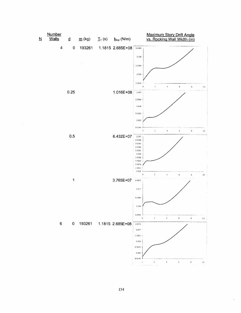
NumberN Walls d m (kg) l (s) htop (N/m)
Maximum Story Drift Anglevs. Rocking Wall Width (m)
4 0 193261 1.1815 2.685E+08 00065
3 055
3305
00045
0.0055
33351
33366
3 0064
333062
3,0054
i 1j,-3335 4
2
3 0075
3 335
0 0055
6 0 193261 1.1815 2.685E+083 0065
3337
3 3365
13
154
0.25 1.016E+08
13
0.5 6.432E+07
10
1 3.765E+07
13
6 8
4
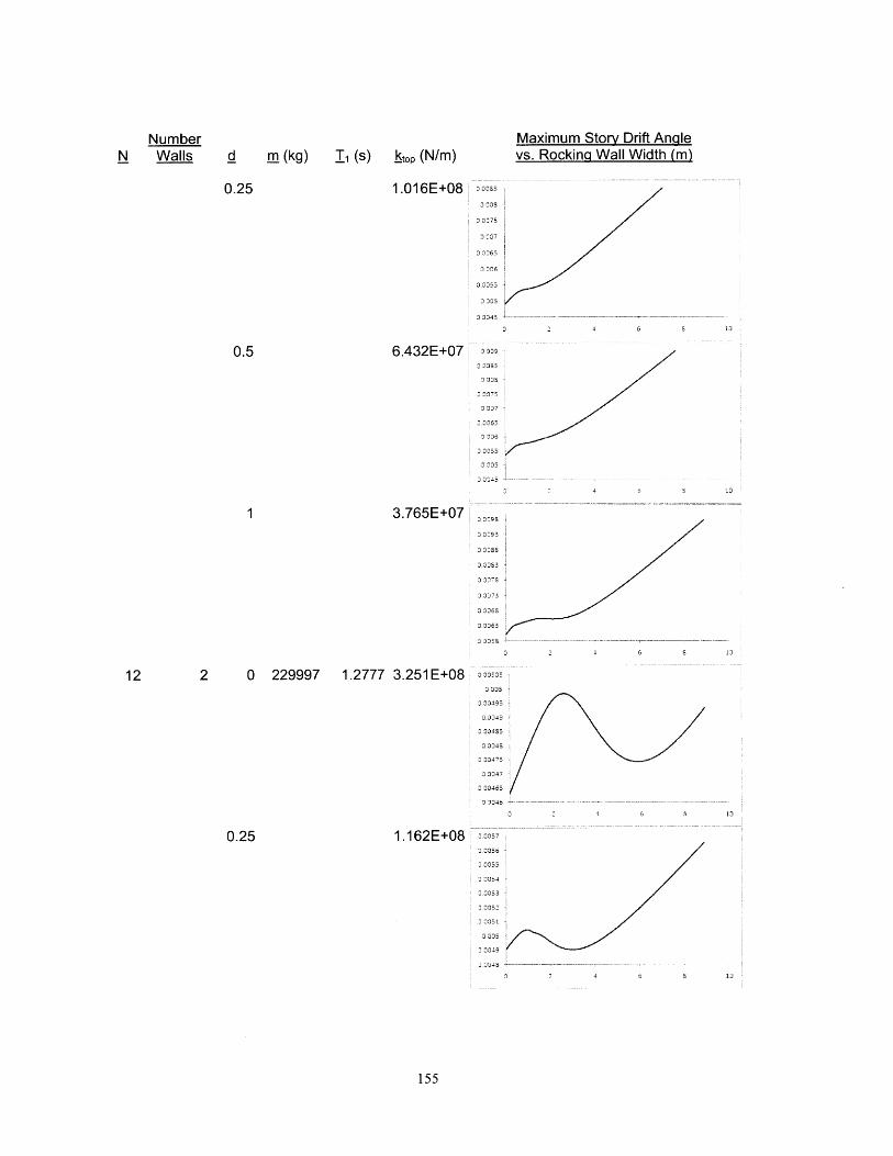
NumberN Walls d im (kg) i (s) ktop (N/m)
Maximum Story Drift Anglevs. Rockinq Wall Width (m)
1.016E+08 103951 n1s
30005
3 DO55
3')05
0 0345~
0.5 6.432E+07
1 3.765E+07
2 0 229997 1.2777 3.251E+08
109
10055
303053 305
3 00475
0 307
3 0045333J95
3346
1.162E+08 00057
3 054
3 005
03134339
30049
13
155
0.25
13
12
13
0.25

NumberN Walls d m (kg) i (s) stop (N/m)
0.5 7.264E+07
1 4.21 OE+07
Maximum Story Drift Anglevs. Rocking Wall Width (m)
0 0057
0 0055
0 053,
j 3352
30062
00061
0,0059
3 0058
0 00550 0054-
4 0 229997 1.2777 3.251E+08
S a 4 6
10
13
0 0051
a 0049
a 0047a 3349
0 0045
0,34
0 0-1
a 0a65
0.25 1.162E+08
0.5 7.264E+07
a 0045
0004
0.0064
0 0058
0 0054
0.005 --
a aa5
156
4 6 19
-r------,-
6 8

d m (kg) _I (s) kop (N/m)
1 4.21 OE+07
6 0 229997 1.2777 3.251 E+08
0 006
0 0061
0 00591
3 3355
3306
3 03
0.25
0.5
1
1.162E+08 o
0 00753376
3 33-55
0 00F5
331
3 0045
7.264E+07'
3 0075
D3035 +-
4.21 OE+0735
0 3075
'1307
3 3b~
3 346
3 3466
157
NumberN Walls
Maximum Story Drift Anglevs. Rocking Wall Width (m)
4 638 10
10
13
13
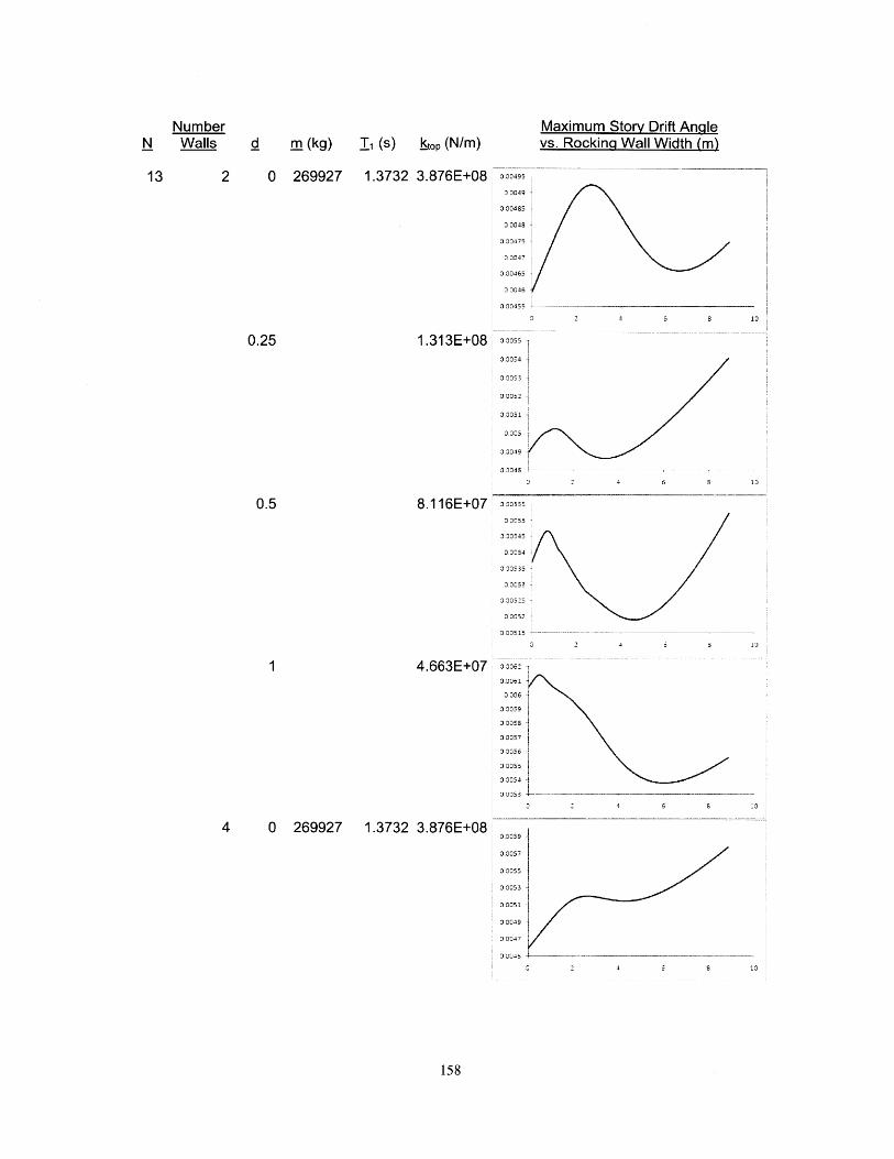
NumberN Walls d _m (kg) _i (s) ltop (N/m)
Maximum Story Drift Anglevs. Rocking Wall Width (m)
2 0 269927 1.3732 3.876E+08
2 4 6 8
4 0 269927 1.3732 3.876E+08
13
8 10
13
-
0 2 4 6 8
13 000495
30049
0 00485
00048
3 30475
0 00475
0 0046
0 00455
0.25 1.313E+08
0.5
3 00550 0054
0 0053
OM052
0.005
3,3355
03348
3 00555
0 30555
0 00545
333054
3 30350 00535
0 0052
0 00515
8.116E+07
1 4.663E+07 000623,3361
0 00830359
333055
3 0358
0 0357
3 3356
0 0054
3 0053
0.00519
313357
3 3355
313353
0.0049
0 0047
30045
13
158
4 10

NumberN Walls d m (kg) i (s) kp (N/m)
1.313E+080.25
0.5
Maximum Story Drift Anglevs. Rocking Wall Width (m)
3 0064
3 3063
3 0058
000503~
005i
0039
8.116E+07
6 0 269927 1.3732 3.876E+08
0005--9
4 4365
3 3366
0064
3 3394
000634
3 3059
0,0058 - - - - - --
3 33~
3 3j6~
330055
0045
33700075
0 007
0 0053) 3364
13
159
13
1 4.663E+07
13
13
0.25 1.313E+08
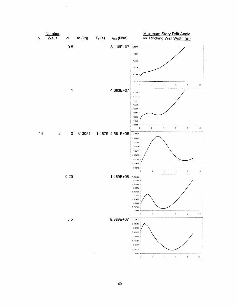
NumberN Walls d rm (kg) i (s) stop (N/m)
0.5 8.116E+07
1 4.663E+07
Maximum Story Drift Anglevs. Rocking Wall Width (m)
00075
0 007
00065
0 0055
0 0074
00072
3 003833066
300364
33363
3 358
3 2
00043
0004853 0345
3 00475
3003465
0 00455
00012
1.469E+08 000325
3 3352
3 00515
0.0049
0 00485
0 004841
8.989E+07 0 00550 03545
0 0054
0.0053500053
0 005250 0052
00515
0.005113
160
10
14 2 0 313051 1.4679 4.561E+08
0.25
0.5
4 10
10

Number Maximum Story Drift AnqleN Walls d m (kg) _I (s) htop (N/m) vs. Rockinq Wall Width (m)
1 5.124E+07 63 2361
3 0059
3 0357
0 0056
0 0053
3 2 4 6 13
4 0 313051 1.4679 4.561 E+08 0 0056
3.0354
33
200430 0046
3 2 4 6 1 13
0.25 1 .469E+08
3 049
30147
3 2 4 4 13
0.5 8.989E+'07 6
3 0058
33374
0 0056
0 0054
3 0052-9 -3331047
3 2 4 s 13
1 5.124E+07 33367
3 3364
33361
32316
3 0056040063
0 0057 -- - -
0 8 1
161
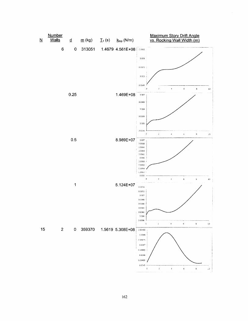
NumberN Walls d _m (kg) _I (s) stop (N/m)
Maximum Story Drift Anglevs. Rockinq Wall Width (m)
6 0 313051 1.4679 4.561E+08
0.25 1.469E+08
2 265
0 0053
0.0055
22245 -,
2 2 4 6 8
0007
2.0055
2 2245 4-
~120.5 8.989E+07 0,337
2 3368
2 30s6
0.3064
33062
3 335
3 005S
32256
2 2354
3,3052 i
o 12
1 5.124E+07
2.00682 2266
3 0064
0.0062
222658206
2 0 359370 1.5619 5.308E+08
13
162
13
150.0048
2330475
0,0047
1.00465
0.0046
0.00455/
00045
13

NumberN Walls d m (kg) _I (s) ktop (N/m)
Maximum Story Drift Anglevs. Rockina Wall Width (m)
1.629E+08 3331
0.00495
0 0049
3.00485
3 3045
3004475
10
9.879E+07
0.25
0.5
13
1 5.592E+07
4 0 359370 1.5619 5.308E+08
0.25 1.629E+08
3 062
3.0059
3 0053
3 0051
32 4 6 S
3 3355
O.0052
0 0351
3 03347
3 0346
1,0045
3 0045
0 4 6 S
3,0057
3 00O55
30053
0 0051
3 0045
3 3047
3 00453 2 4 6 8S
163
003355
3.03545
3 3354
3 3351
3 3053,
13
10
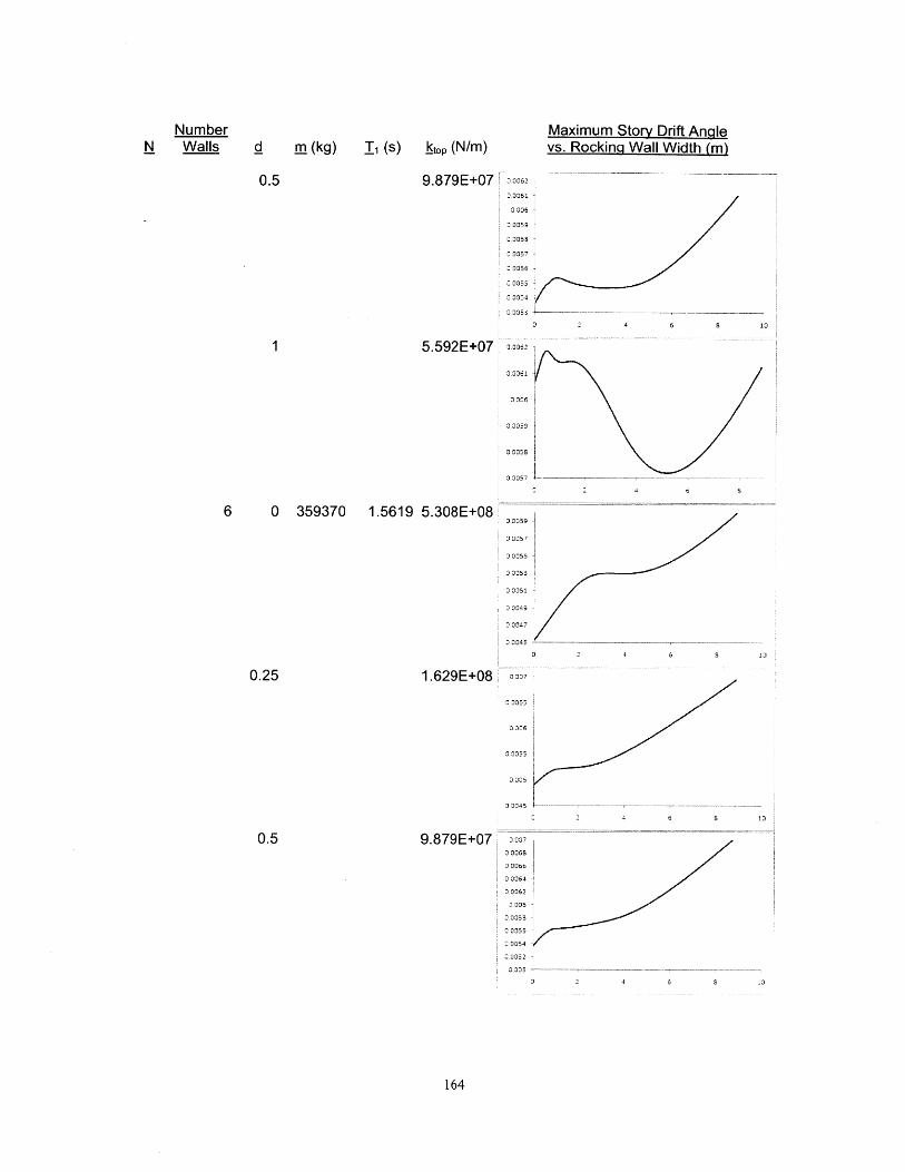
NumberN Walls d m (kg) I (s) htop (N/m)
Maximum Story Drift Anglevs. Rocking Wall Width (m)
9.879E+07 33062
0 0061 1
.005
0,0057
o 0056/00055
0 0054
0 0053
5.592E+07 6
00059
0 0058
00057 L
3305
6 0 359370 1.5619 5.308E+08
0 0057
3 0331
0 0049
0 0047
3 0045
1.629E+08 0007
0 0063
006
0.005
0045-
9.879E+070004,
30066
0 0062
0 0058
3 005430354
0.00 - -
3 2 4 6 S
0.5
1
10
0.25
10
0.5
10
13
164
6 8
4 6
4
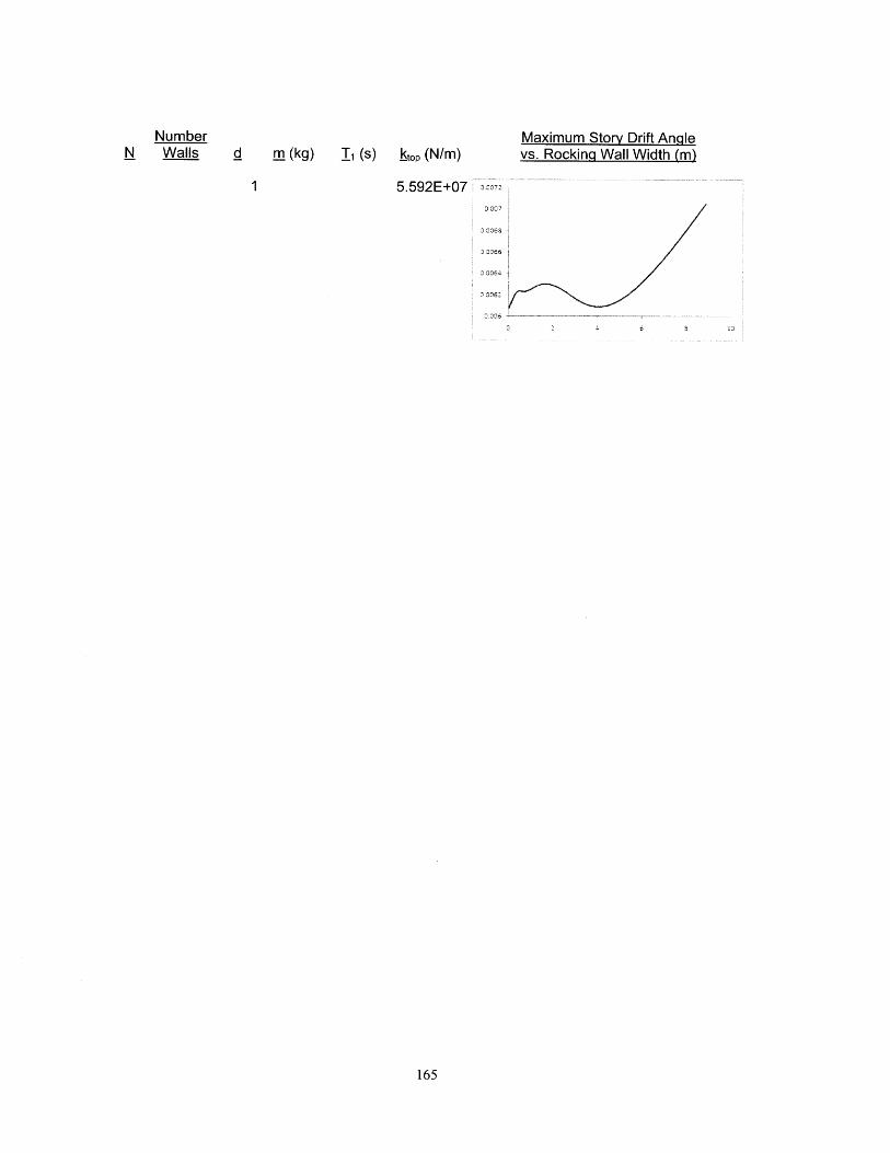
NumberN Walls d m (kg) i (s) htop (N/m)
Maximum Story Drift Anglevs. Rocking Wall Width (m)
5.592E+07 0.17
03075
3 35bS
033C64
033
13
165
1

166

Appendix C: MATLAB Code for Solving the Rocking Wallas a Flexible Continuous System, using Lagrange,as in Section 3.6.
syms x L h kl k2 rho A m EI qO ql qOdot qldot q0dotdot qldotdot;
Building nodes are numbered from the top down. The top node is 1.
This is unlike the work body, in which the top-node-N convention is used.
This example demonstrates the method for a two-story model.
The model expects the building shape to follow the wall shape (rigid links),
so expects L to be about the same as h * number storys or greater
replace syms with values
number storys = 2;
wallwidth = 14.4 * 0.3048; % m
walldepth = 2 * 0.3048; % m
m = 57000; % kg
concretemodulus = 24.82*10^9; % Pa
rho = 2400; % kg/m^3, density of wall
h = 12 * 0.3048; % m, height of 1 story
kl = 8*12*concretemodulus*((0.3048)^4/12)/h^3;
k2 = kl; % 35.0237776 MN/m
L = numberstorys * h;
wallI = walldepth*wallwidth^3/12;
EI concrete modulus*wallI;
A = wallwidth*wall depth;
I alpha factor for psil
a = 5*pi/4/L;
% trial functions
psiO = x/L;
psil = sin(a*x);
% position function u(x,t)
u = psio*qO + psil*ql;
% find u at critical locations
u_1 = subs(u,x,2*h);
u_2 = subs(u,x,h);
% building stiffness matrix
K_building = [kl -kl;-kl kl + k2];
% find loads on the wall from the building
P = K-building*[ul;u_2];
% BUT! these forces are in the -ve direction on the wall
167

% when the movements by the wall are +ve. So we want the -ve of these forces.
% Check this by looking at the force vector P. For an all-positive mode
such as rigid body rotation (qO), you want the force to be -ve WRT qO.
P -P;
p1 P(1);
p2 P(2);
% 'differentiate' u wrt t by substituting the q functions with qdot
udot = subs(u,qO,qOdot);
udot = subs(udot,ql,qldot);
find udot at critical locations
udoth = subs(udot,x,h);
udot_2h = subs(udot,x,2*h);
% differentiate u wrt x
dudx = diff(u,x);
d2udx2 = diff(dudx,x);
energy functions for Lagrange
K_forlumped_masses = 1/2*m*udot_h^2 + 1/2*1/2*m*udot_2h^2;
K 1/2*rho*A*int(udot^2, x, 0, L) + K_forlumped masses;
V = 1/2*EI*int(d2udx2^2, x, 0, L);
%(NB: there is no curvature associated with the rigid body mode
% so d2udx2 & thus V are not functions of qO)
W = 1/2*pl*u_1 + 1/2*p2*u_2; % is this definitely 1/2?
% differentiate energy functions
dKdqOdot = diff(K,qOdot);
ddtdKdqOdot = subs(dKdqOdot,qOdot,qOdotdot); % differentiation wrt t by substitution
ddtdKdqOdot = subs(ddtdKdqOdot,qldot,qldotdot); % differentiation wrt t by substitution
dKdqldot = diff(K,qldot);
ddtdKdqldot = subs(dKdqldot,qOdot,qOdotdot); % differentiation wrt t by substitution
ddtdKdqldot = subs(ddtdKdqldot,qldot,qldotdot); % differentiation wrt t by substitution
dKdqO = diff(K,qO);
dKdql = diff(K,ql);
dVdqO = diff(V,qO);
dVdql = diff(V,ql);
dWdq0 = diff(W,qO);
dWdql = diff(W,ql);
% get the matrix components
(differentiation only works for this because there
are no higher powers/functions of qO, qOdotdot, etc)
Mll = diff(ddtdKdq0dot,q0dotdot);
M12 = diff(ddtdKdq0dot,qldotdot);
M21 = diff(ddtdKdqldot,q0dotdot);
M22 = diff(ddtdKdqldot,qldotdot);
168
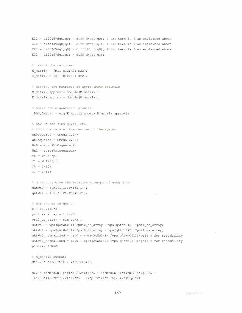
K11 = diff(dVdqO,qO) - diff(dWdqO,qO); % 1st term is 0 as explained above
K12 = diff(dVdqO,ql) - diff(dWdqO,ql); % 1st term is 0 as explained above
K21 = diff(dVdql,qO) - diff(dWdql,qO); % 1st term is 0 as explained above
K22 = diff(dVdql,ql) - diff(dWdql,ql);
create the matrices
M_matrix = [M11 M12;M21 M22];
K_matrix = [K11 K12;K21 K22];
display the matrices as approximate decimals
M_matrixapprox = double(Mmatrix);
K-matrixapprox = double(K matrix);
solve the eigenvector problem
[Phi,Omega] = eig(Kmatrixapprox,M_matrix_approx);
now we can find q0,ql, etc.
find the natural frequencies of the system
Wn0squared = Omega(1,1);
Wnlsquared = Omega(2,2);
WnO = sqrt(Wn0squared);
Wnl = sqrt(Wnlsquared);
f0 = Wn0/2/pi;
fl = Wnl/2/pi;
TO = 1/fO;
T1 = 1/fl;
c vectors give the relative strength of each mode
qAtWnO = [Phi(l,l);Phi(2,1)];
qAtWnl = [Phi(1,2);Phi(2,2)];
% sub the qs to get u
x = 0:0.1:2*h;
psiO as array = 1.*x/L;
psil as array = sin(a.*x);
uAtWnO = vpa(qAtWnO(1))*psiOasarray + vpa(qAtWnO(2))*psilas array;
uAtWnl = vpa(qAtWnl (1) )*psiOasarray + vpa(qAtWnl (2)) *psil as array;
uAtWnOnormalized = psiO + vpa(qAtWnO(2))/vpa(qAtWnO(1))*psil % for readability
uAtWnlnormalized = psiO + vpa(qAtWnl(2))/vpa(qAtWnl(l))*psil % for readability
plot(x,uAtWnO)
M matrix output:
Mll=(3*h^2*m)/L^2 + (A*L*rho)/3
M12 = (h*m*sin((5*pi*h)/(2*L)))/L + (h*m*sin((5*pi*h)/(4*L)))/L -
(A*rho*((16*2^(1/2)*L)/25 - (4*pi*2^(1/2)*L)/5))/(2*pi^2)
169

M21 = (h*m*sin((5*pi*h)/(2*L)))/L + (h*m*sifl((5*pi*h)/(4*L)))/L -
(A*rho*((16*2^~(1/2)*L)/25 - (4*pi*2 ~(1/2)*L)/5))/(2*piA2)
M22 = (m*sin((5*pi*h)/(2*L))V2)/2 + m*sin((5*pi*h)/(4*L) )A2 + (A*rho*(L -
(2*L) /(5*pi)) )/2]
170

Appendix D: MATLAB Code to Find the Stiffness Matrix of Building-Rocking Wall System
building nodes are numbers from the bottom up. the top node is N.This is like the work body, in which the top-node-N convention is also used.Get input
N = input('Number Stories: ');L = input('Total Height (m): ');EIwall = input('EI of Wall (Nm^2):bldg storey stiffness = input('Building Storey Stiffness (N/m): ');if (isempty(N))N=ll;end; if (isempty(L))L=33;end; if (isempty(EI wall))EI wall=1000000;end; if(isempty(bldgstoreystiffness) )bldg storey stiffness=1000000;end;
% wall stiffness matrixF wall prime = zeros(N-1,N-1);for i = 1:N-1; ' i is point measured
for j = 1:N-1; % j is point of application of loadx = (i-2)/N*L; the distance to the point measured from the cantilever roota = (j-2)/N*L; % distance to point of application of load from cantilever root
find the rotation termmoment-arm = a;single storey height = L/N;distance-to-point measured from cantilever root = x;rotation at lowest storey = momentarm*singlestorey height/(3*EI wall);rotation-term = rotation at loweststorey*distance to pointmeasured from cantilever root;
% find the cantilever termif (i > j)
must use the x > a cantilever formulacantileverterm = a^2/(6*EIwall)*(3*x - a);
elsemust use the x <= a cantilever formula
cantilever-term = x^2/(6*EI wall)*(-x + 3*a);end;F wall prime(i,j) = rotation-term + cantilever-term;
end;end;K wall prime = inv(F wall-prime);K wall = zeros(N,N);for i = 1:N-1;
for j = 1:N-1;K_wall(i+l,j+l) = K wallprime(i,j);
end;end;
building stiffness matrixSum bldg stiffness = bldg storeystiffness;K bldg = zeros(N,N);for j = 1:N;
diagonalsK_bldg(j,j) = 2*Sum bldgstiffness;
end;for j = 1:N-1;
off diagonalsK bldg(j,j+l)= -Sum bldg stiffness;K_bldg(j+l,j)= -Sum bldg stiffness;
end;K_bldg(N,N)=Kbldg(N,N) - Sum bldg stiffness;
moments matrix
M = zeros(N,N);for j = 2:N;
% top rowM(lj) = -j;
end;
L 1 "linear-1"L 1 = zeros(N,N);for j = 1:N;
start of each rowL l(j,l) = j;
end;
171

total stiffness matrixK total = Kbldg + (M + eye(N))*K-wall*(eye(N) - Lil);
172
Related Documents