Robustness of Nonlinear Regression Methods under Uncertainty:  Applications in Chemical Kinetics Models

Robustness of Nonlinear Regression Methods under Uncertainty:Applications in Chemical Kinetics Models

German Vidaurre, Victor R. Vasquez,* and Wallace B. Whiting

Chemical Engineering Department, University of Nevada-Reno, Reno, Nevada 89557

In this work, we study the robustness of nonlinear regression methods under uncertainty forparameter estimation for chemical kinetics models. We used Monte Carlo simulation to studythe influence of two main types of uncertainty, namely, random errors and incompleteexperimental data sets. The regression methods analyzed were least-squares minimization (LSM),maximum likelihood (ML), and a method that automatically reweights the objective functionduring the course of the optimization called IVEM (inside-variance estimation method). Althoughthis work represents a preliminary attempt toward understanding the effects of uncertainty innonlinear regression, the results from the analysis of the case studies indicate that theperformance of the regression procedures can be highly sensitive to uncertainty due to randomerrors and incomplete data sets. The results also suggest that traditional methods of assigningweights a priori to regression functions can affect the performance of the regression unless theseweights correspond to a careful characterization of the residual statistics of the regressionproblem. In the case in which there is no prior knowledge of these weights (particularly inmaximum likelihood regression), we suggest that they be characterized, in a preliminary way,by performing a least-squares minimization regression first or by using a method thatautomatically estimates these weights during the course of the regression (IVEM). We believethat the performance of regression techniques under uncertainty requires attention before aregression method is chosen or the parameters obtained are deemed valid.

1. Introduction

Many different regression strategies can be used tofit experimental data by optimizing the parameters oflinear and nonlinear models. Of particular interest areapproaches that are sufficiently accurate to representphysical or chemical phenomena as well as efficient froma computational standpoint.

For chemical engineering applications (particularlyin the areas of thermodynamics and reaction engineer-ing), parameter regression or estimation is an importantissue. Although generalized linear models play animportant role in many applications, the focus of thepresent work is on nonlinear models, which usuallypresent more challenges and yet are very common inthermodynamics and reaction kinetics. The most com-mon nonlinear regression approaches used for the past20 years are the least-squares minimization (LSM) andmaximum likelihood (ML) methods. Even though thesetwo approaches have been very successful in solvingimportant problems, they present limitations, in par-ticular, in the choice of appropriate weighting factorsand in the definition of the objective function so thatthe values of the regression parameters are properlyoptimized. Additionally, little is known about the per-formance of these methods under uncertainty.

Traditionally, the weighting factors are chosen usingdispersion characterization parameters of experimentalmeasurements such as the standard deviation. Often,the general definiton of the objective function is specific

to the nature of the problem being analyzed. Forinstance, Sørensen et al.1 and Whiting et al.2 present asummary of objective function definitions for the pa-rameter regression of models used in the prediction ofliquid-liquid equilibria that reflects the difficulties inchoosing appropriate regression objective functions forcomplex regression problems.

In this work, we study the impact that the definitionof the regression objective function has on parameterestimation under uncertainty in the experimental data.We compare a method that automatically reweights theobjective function during the course of the optimization3

against more traditional methods such as the LSM andML regression methods.

Two case studies are presented. The first consists offinding the parameters of a kinetic model used todescribe the process of converting methanol into differ-ent hydrocarbons,4-7 and the second is a kinetic modelfor the isomerization of R-pinene into dipentene andallo-ocimen.8-10

The remainder of the paper is organized as follows:Section 2 summarizes some of the basic ideas behindparameter estimation. Section 3 presents a basic de-scription of the regression method introduced byVasquez and Whiting3 and is followed by the casestudies in sections 4 and 5. Section 6 provides con-cluding remarks and describes future work.

2. Parameter Estimation

The estimation of parameters in kinetic models fromtime series data and other data types is essential forthe design, optimization, and control of many chemicalsystems. The models that describe the reaction kinetics

* To whom correspondence should be addressed. E-mail:[email protected]. Tel.: (775) 784-6060. Fax: (775) 784-4764.

1395Ind. Eng. Chem. Res. 2004, 43, 1395-1404

10.1021/ie0304762 CCC: $27.50 © 2004 American Chemical SocietyPublished on Web 02/20/2004

usually take the form of a set of differential algebraicequations. The statistics and model formulation for suchproblems have been widely studied, but the regressionapproach is still a matter of discussion in engineeringapplications.

The accurate prediction of specific kinetic rates is acrucial step in reactor design and other areas such asthe prediction of thermodynamic properties and thedesign of separation processes. For modeling purposes,the following steps are typical: (a) experimental datameasurement, (b) model development, and (c) modelparameter estimation.

The two main sources of uncertainty for the param-eter values are (a) the method used for obtaining theparameters and (b) the experimental data. The othertype that can be important is modeling error, whichquantifies the inability of the model and parametriza-tion chosen to describe perfectly the physical systemunder study. In this work, it is assumed that there isno modeling error.

The uncertainty associated with experimental datais usually described in terms of random and systematicerrors. Often, the quantification of random errors isreduced to the apparatus precision. The systematicuncertainties are conceptually well-defined, but they aretraditionally ignored in regression.3 Such uncertaintiesare mainly caused by calibration errors and changingenvironmental conditions, among others.

In addition to the typical problems encountered withregression objective functions (e.g., multiple localminima), even if the optimization method guaranteesthat the global minimum is found, the parametersobtained are still not optimal if the objective functionis not appropriate. To achieve an accurate prediction,all of the effects of the aforementioned errors have tobe minimized or taken into account.

The most common approach used to define regressionobjective functions is to minimize the sum of the squareddifferences between the experimental and predictedvalues (LSM) or to maximize the probability that theresidual statistics of the model predictions correspondto the probability distribution of the uncertainty presentin the experimental data (ML).

Starting with a data set of n observations for mdependent variables denoted as (xij, yij), where i ) 1, 2,..., n, and j ) 1, 2, ..., m, and where the array x denotesa vector of independent variables, the first approach(LSM) consists of finding the values of the modelparameters θ such that the following function is mini-mized

where εij represents the error of the model prediction

Assuming that the joint probability distribution of εij isknown, then the maximum likelihood estimate of θ isobtained by maximizing the likelihood function that bestreproduces the joint probability distribution of εij. Sup-pose that the εij are independent and identically dis-tributed for a fixed dependent variable j, with a densityfunction σj

-1gj(εij/σj), so that gj is the standardized error

probability distribution of unit variance. Then, thelikelihood function is defined as

If the εij’s are independent and identically normallydistributed for a fixed dependent variable j, then thefunction gj is given by

and the logarithm of eq 3 becomes

In this likelihood function, σj2 is the variance, or error

term, which cannot be estimated from the experimentaldata, given that it is a function of the predictedresiduals. Herein lies the difference between traditionalapproaches and the method proposed by Vasquez andWhiting.3 For nonlinear regression, traditional ap-proaches assume a priori estimation of the varianceσj

2 based on experimental precision. However, suchan approach is internally inconsistent becausethis estimate is not equal to the final values ob-tained from the residuals at the end of the regressionprocedure.

S(θ) ) ∑j

m

∑i

n

[yij - fj(xij,θ)]2 (1)

yij ) fj(xij,θ) + εij (2)

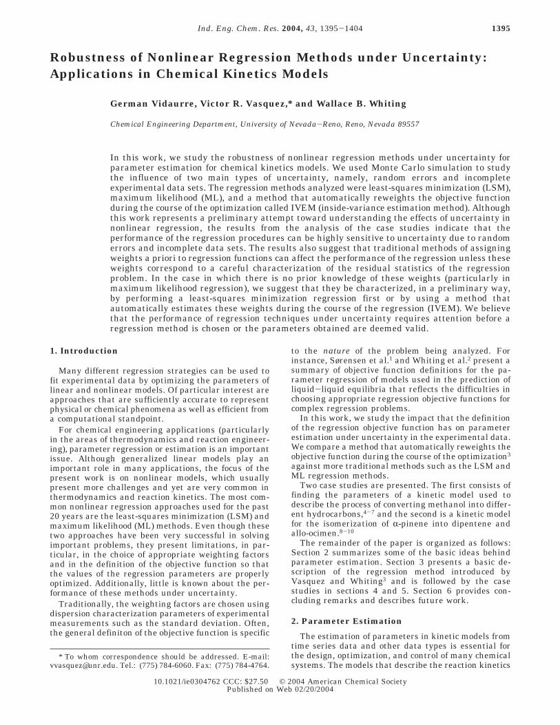
Figure 1. Typical synthetic data set generated by eq 10 and usedto regress the parameters of the model given by eq 7. The curvescorrespond to the predictions of the parameters given by Maria.4Plotted are the profiles of the species A (4), C (O), and P (/).

Table 1. Regressed Parameter Sets for the Kinetic Model(Eq 7) Describing the Methanol to HydrocarbonConversion Process

θ̂itrueθi/ IVEMa MLa LSMa IVEMb MLb LSMb

2.69 3.145 3.211 3.182 3.174 3.189 3.1790.50 0.373 0.848 0.712 0.041 0.269 0.4403.02 3.457 3.052 3.166 3.783 3.596 3.5000.50 0.232 0.054 0.006 0.698 0.594 0.4920.50 1.628 1.980 1.944 3.990 4.819 4.634

a Entire data set used in the regressions. b Only the first halfof the data set used in the regressions.

p(yij|θ,σ2j) ) ∏

j

m

∏i

n [σj-1gj(yij - fj(xij,θ)

σj)] (3)

gj(xij,yij) ) 1

σjx2πexp{- 1

2[yij - fj(xij,θ)]2

σ2j

} (4)

-log p(yij|θ,σ2j) )

mn

2log 2π +

n

2log ∏

j

m

σ2j +

1

2∑

j

m

∑i

n [yij - fj(xij,θ)

σj]2

(5)

1396 Ind. Eng. Chem. Res., Vol. 43, No. 6, 2004

The method of Vasquez and Whiting3 called IVEM(inside-variance estimation method) consists of using eq5, but instead of using a priori values of the variancesσj, obtaining these values from each iteration of theoptimization procedure using the residual distributionof the estimates. Thus, at the end of the optimizationprocess, the statistical properties of the residual distri-bution of the estimates are consistent with the varianceused in the maximum likelihood function, guaranteeingthe most likely values of the parameters, assuming thatthere is no modeling error and, therefore, that theresiduals are Gaussian.

For the case in which there is significant modelingerror, the form of the function gj in eq 3 is no longerGaussian. One should, in principle, know a valid formof gj(εij/σj) to define the likelihood function. However,eq 5 coupled with the IVEM approach still presents asignificant advantage when compared to traditionalregression approaches in the sense that the objectivefunction is always reweighted according to the estimatesof the residuals.

3. IVEM Algorithm

Here, we describe the basic algorithm of the IVEMregression methodology (for more details, see Vasquezand Whiting3). The algorithm starts with an appropriateinitial guess for the parameters. A good estimate is

essential for rapid convergence of the algorithm. Ingeneral, the IVEM algorithm exhibits slower conver-gence than more traditional regression methods. Thealgorithm is summarized as follows:

1. Initialize variables.2. Input experimental data.3. Input initial guess θ.4. Compute estimates of the dependent variables

using the current value for θ.5. Compute the sum of the square of the error, where

the error is defined as the difference between thepredicted and experimental value for each dependentvariable.

6. Compute the variance of the errors for eachdependent variable.

7. Evaluate the objective function as defined by eq 5.8. If the objective function has reached a minimum,

store the current value of θ. If not, change θ accordingto the optimization procedure being used and go to step4.

9. Repeat steps 4-8 until the minimum of theobjective function is reached.

4. Illustrative Case Study: Conversion ofMethanol to Hydrocarbons

For the conversion of methanol to hydrocarbons,many kinetic models have been proposed. Themodel analyzed here (see Maria,4 Chang,6 and Anthony5

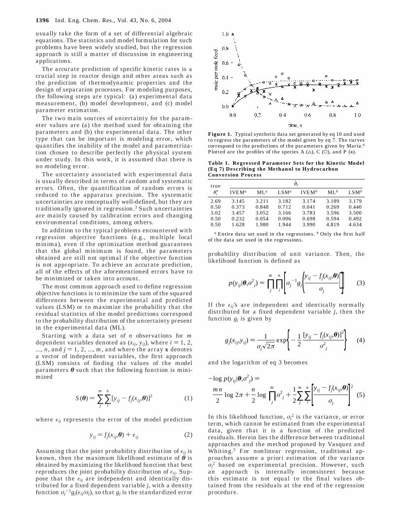
Figure 2. Performance comparison of the mean errors andstandard deviations in the predictions of the concentrations of thespecies A, C, and P of the kinetic model given by eqs 7-9,respectively. The comparison is for the regression methods LSM()), ML (0), and IVEM (4) using complete data sets (no simulationof missing data; see methanol to hydrocarbons case study fordetails).

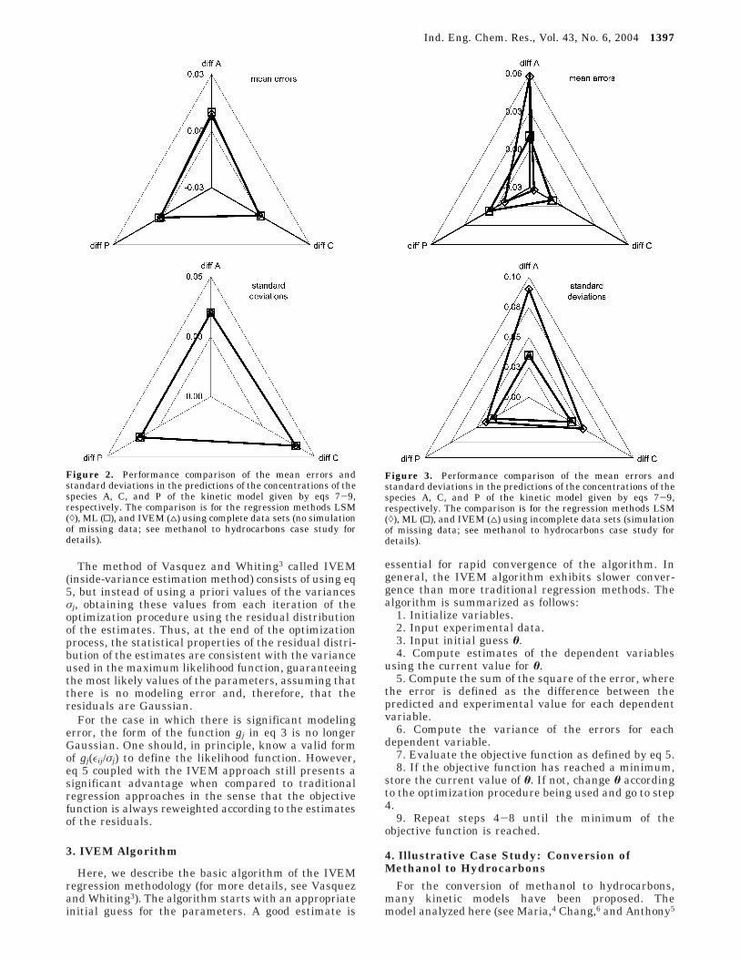
Figure 3. Performance comparison of the mean errors andstandard deviations in the predictions of the concentrations of thespecies A, C, and P of the kinetic model given by eqs 7-9,respectively. The comparison is for the regression methods LSM()), ML (0), and IVEM (4) using incomplete data sets (simulationof missing data; see methanol to hydrocarbons case study fordetails).

Ind. Eng. Chem. Res., Vol. 43, No. 6, 2004 1397

for details) is as follows

where A denotes oxygenates (without water); B de-notes carbenes (C̈H2); C denotes olefins; and P denotesparaffins, aromatics, and other products. The constantsk1-k6 are the specific rates of reaction and the param-eters to be regressed.

Maria4 assumed only first-order reactions and aconstant carbene concentration for isothermal reactionconditions. Considering the quasistationary hypothesis5

and eliminating B, it is possible to obtain the model

where A and C denote the concentrations of componentsA and C, respectively; k23 ) k2/k3; and k63 ) k6/k3. Notethat, in this arrangement, there are only five regressionparameters instead of six.

Regressions for obtaining the model parameters (k1,k4, k6, k23, k63) were performed using three different

approaches: least-squares minimization (LSM), maxi-mum likelihood (ML), and the inside-variance estima-tion method (IVEM). The main objective of this workwas to study the performance of these regressionmethods under uncertainty. Therefore, the methodologyin this case study consisted of taking the set of param-eters that gives the best fit of the experimental data asthe true parameters (notice that this is an artificialconstruct to facilitate the stochastic analysis of thisproblem). Then, using these “true” parameters, one cangenerate predictions of the measured quantities (yij) andadd Gaussian noise to simulate the effect of uncertaintyin the experimental data. Many synthetic data sets canbe generated in this way with different levels of uncer-tainty that can be used to regress the parameters of themodel (θ̂) and compare the results against the true setθ*. The true parameter set used in this example isreported by Maria,4 θ* ) (2.69, 0.5, 3.02, 0.5, 0.5), withall of the values in appropriate dimensions accordingto the rate equations. The Gaussian error is added asfollows

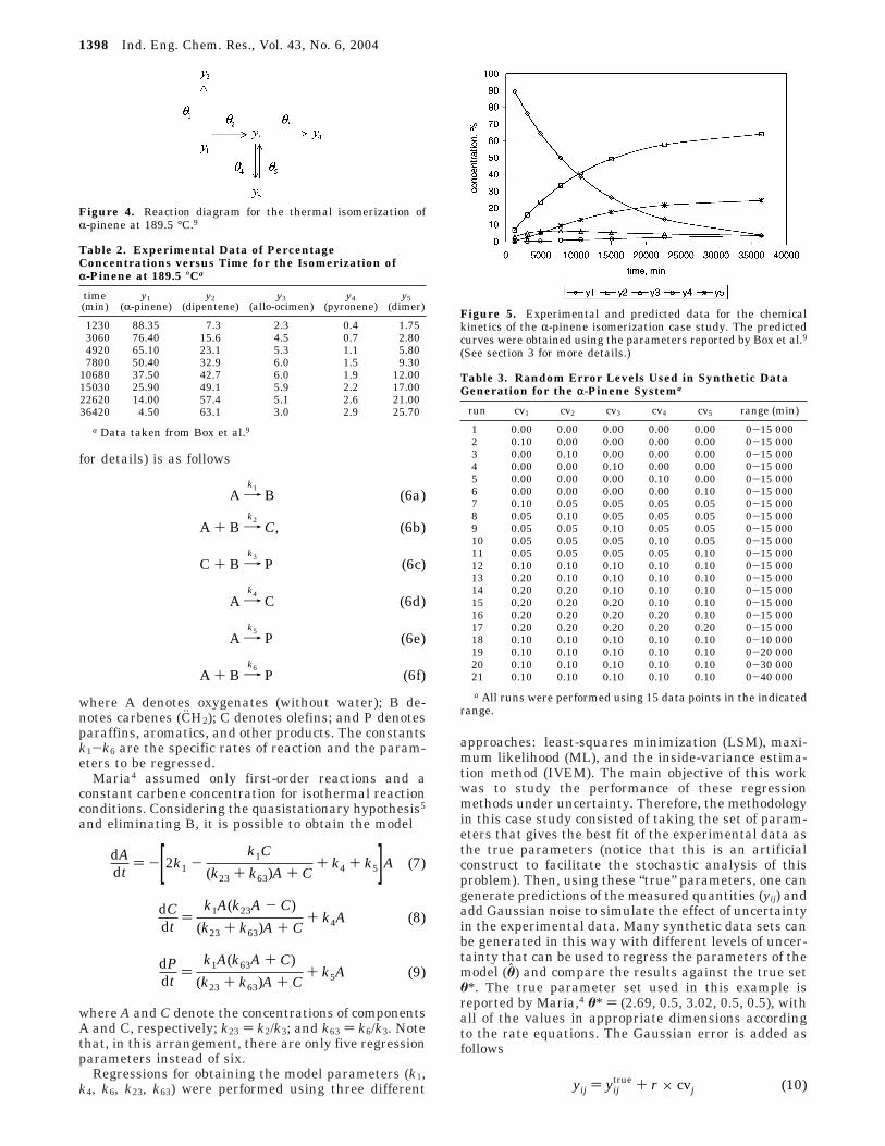
Figure 4. Reaction diagram for the thermal isomerization ofR-pinene at 189.5 °C.9

Table 2. Experimental Data of PercentageConcentrations versus Time for the Isomerization ofr-Pinene at 189.5 °Ca

time(min)

y1(R-pinene)

y2(dipentene)

y3(allo-ocimen)

y4(pyronene)

y5(dimer)

1230 88.35 7.3 2.3 0.4 1.753060 76.40 15.6 4.5 0.7 2.804920 65.10 23.1 5.3 1.1 5.807800 50.40 32.9 6.0 1.5 9.30

10680 37.50 42.7 6.0 1.9 12.0015030 25.90 49.1 5.9 2.2 17.0022620 14.00 57.4 5.1 2.6 21.0036420 4.50 63.1 3.0 2.9 25.70

a Data taken from Box et al.9

A 98k1

B (6a)

A + B 98k2

C, (6b)

C + B 98k3

P (6c)

A 98k4

C (6d)

A 98k5

P (6e)

A + B 98k6

P (6f)

dAdt

) -[2k1 -k1C

(k23 + k63)A + C+ k4 + k5]A (7)

dCdt

)k1A(k23A - C)

(k23 + k63)A + C+ k4A (8)

dPdt

)k1A(k63A + C)

(k23 + k63)A + C+ k5A (9)

Figure 5. Experimental and predicted data for the chemicalkinetics of the R-pinene isomerization case study. The predictedcurves were obtained using the parameters reported by Box et al.9(See section 3 for more details.)

Table 3. Random Error Levels Used in Synthetic DataGeneration for the r-Pinene Systema

run cv1 cv2 cv3 cv4 cv5 range (min)

1 0.00 0.00 0.00 0.00 0.00 0-15 0002 0.10 0.00 0.00 0.00 0.00 0-15 0003 0.00 0.10 0.00 0.00 0.00 0-15 0004 0.00 0.00 0.10 0.00 0.00 0-15 0005 0.00 0.00 0.00 0.10 0.00 0-15 0006 0.00 0.00 0.00 0.00 0.10 0-15 0007 0.10 0.05 0.05 0.05 0.05 0-15 0008 0.05 0.10 0.05 0.05 0.05 0-15 0009 0.05 0.05 0.10 0.05 0.05 0-15 00010 0.05 0.05 0.05 0.10 0.05 0-15 00011 0.05 0.05 0.05 0.05 0.10 0-15 00012 0.10 0.10 0.10 0.10 0.10 0-15 00013 0.20 0.10 0.10 0.10 0.10 0-15 00014 0.20 0.20 0.10 0.10 0.10 0-15 00015 0.20 0.20 0.20 0.10 0.10 0-15 00016 0.20 0.20 0.20 0.20 0.10 0-15 00017 0.20 0.20 0.20 0.20 0.20 0-15 00018 0.10 0.10 0.10 0.10 0.10 0-10 00019 0.10 0.10 0.10 0.10 0.10 0-20 00020 0.10 0.10 0.10 0.10 0.10 0-30 00021 0.10 0.10 0.10 0.10 0.10 0-40 000

a All runs were performed using 15 data points in the indicatedrange.

yij ) yijtrue + r × cvj (10)

1398 Ind. Eng. Chem. Res., Vol. 43, No. 6, 2004

where r is a Gaussian random deviate with mean 0 andvariance 1, cvj is the assumed maximum level of errorfor the dependent variable j, yij

true represents the valuespredicted by the true parameters θ*, and yij corresponds

to the simulated experimental data. A maximum cvvalue of 0.1 was used for this case study. A typicalsynthetic data set is presented in Figure 1 together withthe true data (continuous lines).

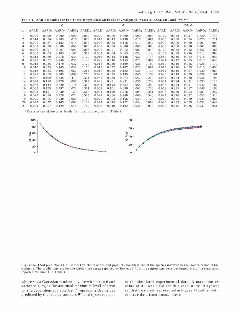
Table 4. AARD Results for the Three Regression Methods Investigated, Namely, LSM, ML, and IVEMa

LSM ML IVEM

run AARD1 AARD2 AARD3 AARD4 AARD5 AARD1 AARD2 AARD3 AARD4 AARD5 AARD1 AARD2 AARD3 AARD4 AARD5

1 0.000 0.000 0.000 0.000 0.000 0.000 0.000 0.000 0.000 0.000 0.169 0.338 0.027 0.720 0.7732 0.014 0.054 0.205 0.016 0.033 0.015 0.043 0.130 0.018 0.087 0.000 0.000 0.024 0.075 0.2113 0.021 0.037 0.182 0.014 0.027 0.020 0.028 0.116 0.011 0.037 0.000 0.000 0.000 0.001 0.0004 0.000 0.000 0.000 0.000 0.000 0.000 0.000 0.000 0.000 0.000 0.000 0.000 0.000 0.001 0.0005 0.000 0.001 0.007 0.001 0.005 0.000 0.001 0.012 0.001 0.010 0.169 0.338 0.042 0.622 0.4666 0.000 0.003 0.103 0.107 0.302 0.001 0.004 0.063 0.033 0.148 0.169 0.338 0.296 0.712 0.9687 0.018 0.550 0.218 0.034 0.129 0.019 0.044 0.138 0.027 0.118 0.016 0.010 0.014 0.018 0.0538 0.027 0.052 0.240 0.035 0.140 0.026 0.040 0.153 0.022 0.089 0.021 0.012 0.015 0.017 0.0489 0.014 0.036 0.170 0.032 0.120 0.013 0.029 0.109 0.026 0.100 0.015 0.010 0.015 0.028 0.11010 0.012 0.035 0.169 0.035 0.150 0.012 0.027 0.107 0.023 0.097 0.013 0.010 0.025 0.015 0.05011 0.012 0.035 0.195 0.067 0.284 0.012 0.028 0.122 0.034 0.138 0.014 0.019 0.017 0.030 0.06312 0.026 0.069 0.305 0.068 0.276 0.026 0.055 0.195 0.040 0.159 0.030 0.018 0.029 0.036 0.10113 0.037 0.109 0.435 0.419 0.371 0.038 0.088 0.274 0.052 0.219 0.034 0.024 0.028 0.036 0.10414 0.048 0.118 0.479 0.098 0.397 0.046 0.97 0.331 0.056 0.234 0.051 0.024 0.031 0.035 0.11515 0.052 0.144 0.620 0.118 0.319 0.051 0.113 0.364 0.068 0.259 0.056 0.024 0.031 0.047 0.18216 0.052 0.129 0.497 0.078 0.311 0.051 0.101 0.330 0.061 0.230 0.059 0.025 0.057 0.048 0.19017 0.050 0.151 0.630 0.129 0.506 0.051 0.120 0.416 0.093 0.351 0.058 0.039 0.054 0.081 0.25218 0.027 0.086 0.428 0.074 0.525 0.027 0.066 0.268 0.060 0.340 0.027 0.016 0.032 0.053 0.31419 0.026 0.066 0.248 0.061 0.195 0.025 0.053 0.166 0.043 0.129 0.027 0.026 0.029 0.035 0.06420 0.027 0.057 0.165 0.062 0.119 0.027 0.049 0.122 0.044 0.094 0.030 0.033 0.025 0.032 0.04221 0.029 0.057 0.129 0.074 0.100 0.029 0.049 0.102 0.044 0.075 0.027 0.046 0.026 0.041 0.041

a Descriptions of the error levels for the runs are given in Table 3.

Figure 6. LSM predictions (100 shown) for the reactant and product concentrations of the species involved in the isomerization of theR-pinene. The predictions are for the whole time range reported by Box et al.,9 but the regressions were performed using the conditionsreported for run 11 in Table 4.

Ind. Eng. Chem. Res., Vol. 43, No. 6, 2004 1399

Two cases were considered: (a) use of 100 data setsof 20 points each generated with eq 10 and (b) use ofthe first half of the synthetic data of case a. The reasonfor using the first half in case b was to study the effectof having incomplete experimental data. This a commonsituation that merits attention regarding the capabilityof the regression method to obtain reasonable param-eters under this type of uncertain conditions. Althoughhaving only the first half of the data set might not becommon, it is still an interesting extreme scenario totest regression methods.

The three objective function definitions described insection 2, namely, LSM, ML, and IVEM, were used toregress the parameters. For the maximum likelihoodmethod, the objective function was the sum of thesquares of the differences between the measured dataand the model prediction for all variables, weighted bythe estimated standard deviation of the differencebetween the experimental data and the data predictedby the least-squares minimization method. The corre-sponding weights in this case are σA ) 0.001 21, σC )0.001 67, and σP ) 0.0119. Notice that, by weighting theobjective function in this way, a better approximationof the residual statistics is already obtained than wouldbe the case using measurement equipment precisionstatistics.

The optimization procedure used was a successiveunidirectional minimization method using the modified

direction set of Powell,11 with the parameters reportedby Maria4 as initial guesses.

The parameter sets regressed by LSM, ML, and IVEMare presented in Table 1 for both cases of using thecomplete synthetic data set in the regressions and usingonly the first half of the data set. Figure 2 summarizesthe general statistical results of this regression for thecase of using the complete data set. The mean error inFigure 2 is defined as the mean of the difference in thepredicted concentrations for species A, C, and P usingthe regressed parameters and the predictions given bythe true parameters θ*, in other words, diff A ) A(θ̂) -A(θ*), diff C ) C(θ̂) - C(θ*), and diff P ) P(θ̂) - P(θ*),respectively (the predicted values of the compositionsare obtained using eqs 7-9). From this figure, weobserve that the three regression methods performreasonably well and give similar results for the param-eters. In this case, the three methods perform well underthe effect of random Gaussian uncertainty only. On theother hand, Figure 3 presents the equivalent of Figure2 but for the case of regressing the parameters usingthe first half of the data set only. It is clear that theLSM method does not perform as well as the other two(i.e., ML and IVEM), which suggests that ML and IVEMtend to be more robust regression methods under thistype of uncertain condition (this is also observed in thenext case study). However, the fact that both ML andIVEM produce similar results is not surprising if we

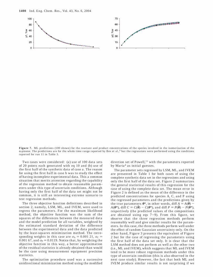
Figure 7. ML predictions (100 shown) for the reactant and product concentrations of the species involved in the isomerization of theR-pinene. The predictions are for the whole time range reported by Box et al.,9 but the regressions were performed using the conditionsreported for run 11 in Table 3.

1400 Ind. Eng. Chem. Res., Vol. 43, No. 6, 2004

recall that the weights used for the ML regressionfunction were obtained from the residual statistics ofthe LSM predictions with respect to the predictions ofthe true parameters. This also indicates the importanceof having good residual statistics if one wants to useML methods with a priori weights. Traditional practiceinvolves the use of weights obtained from the precisionof the measurements, in this case, for the concentrationsof the species A, C, and P. Now, it is not uncommon tofind that the precision statistics can be about the samefor concentration measurements (depending on theexperimental methods used), which will cause theweights (standard deviations of the measurement error)to be equal, thus transforming the ML regressionfunction into an LSM regression case. If the precisionstatistics are different for the concentrations of thedifferent species, then the ML regression function willhave different weights (σj), but there is no guaranteethat these σj’s will correspond to the final statistics ofthe residuals.

There are some important differences between Fig-ures 2 and 3 that are worth mentioning. For the MLmethod, the error present is about 15.8 times largerthan that present when using the entire synthetic dataset in the regression. For the inside-variance estimationmethod, this error is almost the same whether usingthe entire set or just the first half of the synthetic dataset. Reducing the range of the synthetic data set even

more produces a substantial increase in the errorstatistics of the three regression methods. However, asthe range used increases, the effectiveness of the IVEMmethod, indicated by low values of the variances,improves faster than the effectiveness of the other twomethods. In general, it is observed that the error in thepredicted data using the paremeter sets obtained fromthe LSM tend to be the largest.

5. Illustrative Case Study: r-PineneIsomerization

Box et al.9 present an interesting example of acomplex chemical reaction for the thermal isomerizationof R-pinene at 189.5 °C. The chemical reaction is theisomerization of R-pinene (y1) to dipentene (y2) and allo-ocimen (y3). Then, the latter reacts to yield R- andâ-pyrone (y4) and a dimer (y5). The unknown param-eters, θr (r ) 1-5) are the rate constants of thereactions. The reaction scheme is presented in Figure4.

This process was studied experimentally by Fuguitand Hawkins,12 who reported the concentrations of thereactant and the five products (see Table 2). If thechemical reaction orders are known, then mathematicalmodels can be derived to model the concentrations ofthe five chemical species as a function of time.

Hunter and McGregor9 assumed first-order kineticsand derived the following equations for the five products

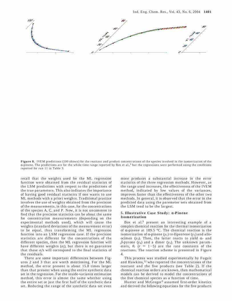
Figure 8. IVEM predictions (100 shown) for the reactant and product concentrations of the species involved in the isomerization of theR-pinene. The predictions are for the whole time range reported by Box et al.,9 but the regressions were performed using the conditionsreported for run 11 in Table 3.

Ind. Eng. Chem. Res., Vol. 43, No. 6, 2004 1401

where y10 is the value of y1 at t ) 0 and

and

The fitting results obtained by Box et al.9 are pre-sented in Figure 5, together with the experimental data.In this work, the parameter set reported by Box et al.9has been assumed to represent the true parameters, θ*) (5.93 × 10-5, 2.96 × 10-5, 2.05 × 10-5, 2.75 × 10-4,4.00 × 10-5), with all values expressed in min-1.

The methodology followed is the same as in theprevious case study, with minor variations. Syntheticdata sets were generated by adding Gaussian randomerror at different levels to what we called the truepredictions of the model according to the followingequation

where r is a Gaussian random number with mean 0 andvariance 1 and cvj is the assumed coefficient of variationfor dependent variable j. The range of cvj used was from0 to 0.2.

Notice that the error introduced by eq 16 is differentfrom that of eq 10 in the previous case study. Equation

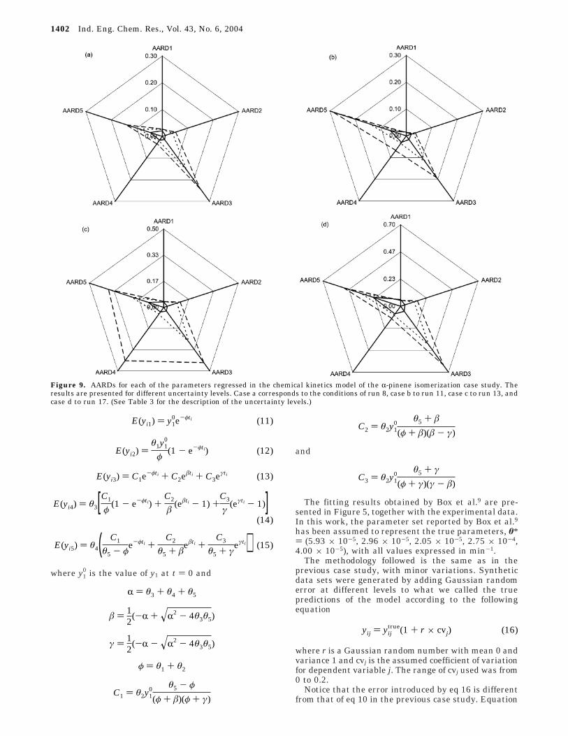
Figure 9. AARDs for each of the parameters regressed in the chemical kinetics model of the R-pinene isomerization case study. Theresults are presented for different uncertainty levels. Case a corresponds to the conditions of run 8, case b to run 11, case c to run 13, andcase d to run 17. (See Table 3 for the description of the uncertainty levels.)

C2 ) θ2y10 θ5 + â

(φ + â)(â - γ)

C3 ) θ2y10 θ5 + γ

(φ + γ)(γ - â)

yij ) yijtrue(1 + r × cvj) (16)

E(yi1) ) y10e-φti (11)

E(yi2) )θ1y1

0

φ(1 - e-φti) (12)

E(yi3) ) C1e-φti + C2e

âti + C3eγti (13)

E(yi4) ) θ3[C1

φ(1 - e-φti) +

C2

â(eâti - 1) +

C3

γ(eγti - 1)]

(14)

E(yi5) ) θ4( C1

θ5 - φe-φti +

C2

θ5 + âeâti +

C3

θ5 + γeγti) (15)

R ) θ3 + θ4 + θ5

â ) 12(-R + xR2 - 4θ3θ5)

γ ) 12(-R - xR2 - 4θ3θ5)

φ ) θ1 + θ2

C1 ) θ2y10 θ5 - φ

(φ + â)(φ + γ)

1402 Ind. Eng. Chem. Res., Vol. 43, No. 6, 2004

16 simulates an error that varies proportionally withthe magnitude of the variable being considered. Thereason for this change with respect to eq 10 is tosimulate situations in which experimental errors varyaccording to the magnitude of the measurements.

Using the so-called true parameters, points weregenerated in the time range of 0-15 000 min (theequivalent of the solid lines in Figure 5), and then 15of them (equally spaced) were chosen to represent ytrue

in eq 16. Other time ranges studied in a similar mannerwere 0-20 000, 0-30 000, and 0-40 000 min. As before,the idea was to evaluate the robustness of the regressiontechniques using incomplete data sets and under theeffect of experimental random Gaussian noise.

To compare the aforementioned methods numerically,a goodness criterion was defined as follows

where θ̂i is an estimator of the ith true parameter θi/

for the kth simulation run. Note that AARDi is not anyof the objective functions used in this work. It is,however, a traditional average absolute relative devia-ton (AARD) measuring the goodness of fit. AARD valueswere calculated to characterize the simulations runs at

the different error levels (cvj) and for the different datasets (yij

true) used.The data subsets used in this work were chosen

arbitrarily (simulation of incomplete experimental data);therefore, many other combinations would be interest-ing as well. Depending on the degree of incompletenessof the data set, there will be cases in which all methodsfail to obtain reasonable values of θ̂ (when comparedagainst θ*), as well as cases in which the best param-eters are obtained depending on the ability of theregression approach to handle the simulated errorimposed.

Different levels of error as well as different combina-tions of these levels were used to analyze the perfor-mance of the regression approaches used. Table 3describes the different error levels used in eq 16 for theuncertain variables yj. The AARD results are presentedin Table 4. The interpretation of these results is betterdescribed by analyzing a specific run. Results corre-sponding to run 11 (see conditions for this run in Table3) are shown in Figures 6-8. We can see the variationof the differents fits obtained by the regression methodsunder study. In general, the IVEM tends to be morerobust than the other two, and as in the first case study,the LSM method seems to be the least robust. This typeof analysis can be done for the other conditions, but ingeneral, the same type of results are observed.

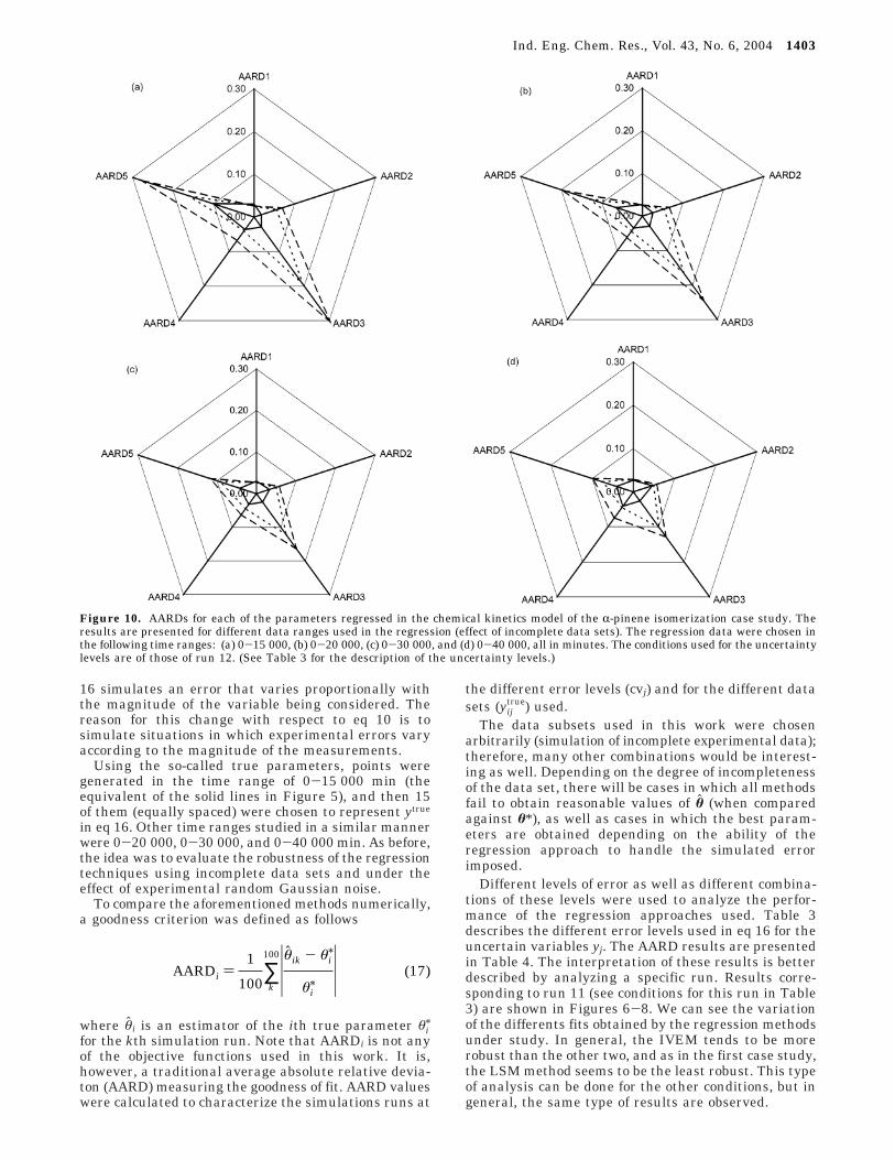
Figure 10. AARDs for each of the parameters regressed in the chemical kinetics model of the R-pinene isomerization case study. Theresults are presented for different data ranges used in the regression (effect of incomplete data sets). The regression data were chosen inthe following time ranges: (a) 0-15 000, (b) 0-20 000, (c) 0-30 000, and (d) 0-40 000, all in minutes. The conditions used for the uncertaintylevels are of those of run 12. (See Table 3 for the description of the uncertainty levels.)

AARDi )1

100∑

k

100|θ̂ik - θi/

θi/ | (17)

Ind. Eng. Chem. Res., Vol. 43, No. 6, 2004 1403

Another way to analyze these results is to plot theAARD values on spider diagrams for the different errorlevels. These diagrams summarize better the perfor-mance of the regression on the predicted variables. Forinstance, Figure 9 shows this type of results for fourdifferent cases of error levels. The error levels usedcorrespond to the conditions of runs 8, 11, 13, and 17(see Table 3) for panels a-d of Figure 9, respectively.In all cases, the IVEM approach is substantially better(from the robustness standpoint) compared to the othertwo. Also notice that the LSM tends to diverge substan-tially faster with increasing the error level. On the otherhand, Figure 10 presents similar results but for the caseof using different ranges for the data sets in theregression. In general, the IVEM approach is morerobust under these circumstances as well, but the othertwo methods improve their performance when the rangein the data set increases (from a to d). The improvementof the ML and LSM methods with increasing range ofthe data sets is not surprising, but it seems that, evenfor the case of using the whole range, IVEM is a morerobust procedure. These results underscore the impor-tance of having good statistics for the residuals inregression problems with uncertain experimental data.

6. Concluding Remarks

The robustness characteristics of traditional regres-sion techniques such as LSM and ML and of a morerecent approach (i.e., IVEM) were studied using twocase studies in the field of chemical kinetics. From theanalysis of the results, it is observed that the perfor-mance of traditional regression methods can be sensitiveto uncertainty in experimental data. This uncertaintymight include, but is not limited to, random andsystematic errors, incomplete data sets, and modelingerrors; in particular, incomplete data sets seem to havesignificant effects on the performance of traditionalregression methods. Maximum likelihood regressionfunctions are usually weighted by the standard errordeviations of the measurements based on equipment orexperimental technique statistics. Depending on thecircumstances (uncertain conditions), this is not alwaysthe best strategy, as shown in the examples studied.Although a priori knowledge of statistics of the residualscan be difficult to obtain, characterizing them by usinga simpler regression model such as LSM and then usingthe results to define the weights in a more sophisticatedapproach such as ML proves to be significantly morerobust than using arbitrary fixed weights in the regres-sion objective function.

The alternative procedure proposed by Vasquez andWhiting3 (IVEM), which automatically reweights thelikelihood function during the course of the optimization,seems to be more robust under uncertain conditions.This method has the advantage of avoiding preliminaryanalyisis (performing preliminary regression using LSMor ML) to characterize the residuals, and it handlesuncertainty better than the other two techniques stud-ied. A drawback of IVEM is the computational conver-gence, which seems to be slower than that of moretraditional methods. A way to improve this behavior isby providing good initial guesses for the parameters

being regressed. Although this work represents a pre-liminary attempt toward understanding the effect ofuncertainty in nonlinear regression, we believe that theperformance of regression techniques under uncertaintyrequires attention before a regression technique ischosen or the parameters obtained are deemed valid.

Future work includes the analysis of other objectivefunction formulations and different applications. Ad-ditionally, assurance tests should be performed toguarantee that the global optimum is found for each ofthe stochastic scenarios. Although such tests are notperformed in this work, the three regression methods(LSM, ML, IVEM) are tested using many stochasticscenarios for two case studies. The general trends orbehaviors of the results are characteristic of the regres-sion methods. Therefore, we believe that the effect ofhaving some scenarios with parameters correspondingto local minima will not drastically change the trendsobserved.

Note Added after ASAP Posting

This article was released ASAP on February 20, 2004.The order of the authors has been changed, and the newversion was posted on February 24, 2004.

Literature Cited

(1) Sørensen, J. M.; Arlt, W. Liquid-Liquid Equilibrium DataCollection; Chemistry Data Series; DECHEMA: Frankfurt/Main,Germany, 1980; Vol. 5.

(2) Whiting, W. B.; Vasquez, V. R.; Meerschaert, M. M. Tech-niques for Assessing the Effects of Uncertainties in Thermody-namic Models and Data. Fluid Phase Equilib. 1999, 158-160,627-641.

(3) Vasquez, V. R.; Whiting, W. B. Regression of BinaryInteraction Parameters for Thermodynamic Models Using anInside-Variance Estimation Method (IVEM). Fluid Phase Equilib.2000 170, 235-253.

(4) Maria, G. An Adaptive Strategy for Solving Kinetic ModelConcomitant Estimation-Reduction Problems. Can. J. Chem. Eng.1989, 67, 825-832.

(5) Anthony, R. G. A Kinetic Model for Methanol Conversionto Hydrocarbons. Chem. Eng. Sci. 1981, 36, 789.

(6) Chang, C. D. A Kinetic Model for Methanol Conversion toHydrocarbons. Chem. Eng. Sci. 1980, 35, 619-622.

(7) Esposito, W. R.; Floudas, C. A. Global Optimization for theParameter Estimation of Differential-Algebraic Systems. Ind. Eng.Chem. Res. 2000, 39, 1291-1310.

(8) Bates, D.; Watts, D. Nonlinear Regression Analysis and ItsApplications; John Wiley and Sons: New York, 1988.

(9) Box, G. E.; Hunter, W. G.; MacGregor, J. F.; Erjavec, J.Some Problems Associated with the Analysis of MultiresponseData. Technometrics 1973, 15 (1), 33-51.

(10) Tjoa, I.; Biegler, L. Simultaneous Solution and Optimiza-tion Strategies for Parameter Estimation of Differential-AlgebraicEquation Systems. Ind. Eng. Chem. Res. 1991, 30, 376-385.

(11) Press: W. H.; Teukolsky, S. A.; Vetterling, W. T.; Flannery,B. P. Numerical Recipes, 2nd ed.; Cambridge University Press:New York, 1994.

(12) Fuguitt, R. E.; Hawkins, J. E. Rate of Thermal Isomer-ization of R-Pinene in the Liquid Phase. J. Am. Chem. Soc. 1947,69, 319.

Received for review June 5, 2003Revised manuscript received September 29, 2003

Accepted January 30, 2004

IE0304762

1404 Ind. Eng. Chem. Res., Vol. 43, No. 6, 2004