Robustly Hedging Variable Annuities with Guarantees Under Jump

Robustly Hedging Variable Annuities with GuaranteesUnder Jump and Volatility Risks

T. F. Coleman, Y. Kim, Y. Li, and M. Patron1

CTC Computational Finance Group

Cornell Theory Center, www.tc.cornell.eduCornell University

NY, U.S.A

Contact: Professor Thomas F. Coleman

Phone: 607 255 9203, Email: [email protected]

(This version: March 17, 2005)

1The authors would like to thank their colleagues Peter Mansfield and Shirish Chinchalkar for manyfruitful discussions. In addition, the authors would like to thank an anonymous referee whose detailedcomments have improved the presentation of the paper.

1

Robustly Hedging Variable Annuities with Guarantees

Under Jump and Volatility Risks

Abstract

Recent variable annuities offer participation in the equity market and attractiveprotection against downside movements. Accurately quantifying this additional equitymarket risk and robustly hedging options embedded in the guarantees of variable an-nuities is a new challenge for insurance companies. Due to sensitivities of the benefitsto tails of the account value distribution, a simple Black-Scholes model is inadequatein preventing excessive liabilities. A model which realistically describes the real worldprice dynamics over a long time horizon is essential for the risk management of thevariable annuities. In this paper, both jump risk and volatility risk are considered forrisk management of lookback options embedded in guarantees with a ratchet feature.

We evaluate relative performances of delta hedging and dynamic discrete risk mini-mization hedging strategies. Using the underlying as the hedging instrument, we showthat, under a Black-Scholes model, local risk minimization hedging is significantly bet-ter than delta hedging. In addition, we compare risk minimization hedging using theunderlying with that of using standard options. We demonstrate that, under a Mer-ton’s jump diffusion model, hedging using standard options is superior to hedging usingthe underlying in terms of the risk reduction. Finally we consider a market model forvolatility risks in which the at-the-money implied volatility is a state variable. Wecompute risk minimization hedging by modeling at-the-money Black-Scholes impliedvolatility explicitly; the hedging effectiveness is evaluated, however, under a joint un-derlying and implied volatility model which also includes instantaneous volatility risk.Our computational results suggest that, when implied volatility risk is suitably mod-eled, risk minimization hedging using standard options, compared to hedging using theunderlying, can potentially be more effective in risk reduction under both jump andvolatility risks.

Key Words: variable annuities, minimum death guarantee, discrete dynamic hedging, riskminimization hedging, jump risk, volatility risk.

1 Introduction

Until the early 1990’s, most variable annuity contracts provided a modest minimum deathbenefit guarantee of return of premiums. This is the greater of the account balance at deathand the sum of the premium deposits, less partial withdrawals, since inception of the contract.The cost of this benefit was considered insignificant and insurance companies did not assessan explicit charge and did not hold an additional reserve for this benefit.

2

Since the middle of 1990’s, variable annuity contracts have offered more substantial mini-mum death benefit guarantees (GMDB). These new guarantees typically include one or moreof the following features [21, 24, 30]:

• Reset: the benefit is the periodically automatically adjusted account balance plus thesum of premium deposits less withdrawals since the last reset date.

• Roll-up: the death benefit is the larger of the account balance on the date of the deathand the accumulation of premium deposits less partial withdrawals accumulated at aspecified interest rate. There may be an upper bound on the benefits.

• Ratchet: the benefit is similar to a reset benefit except that it is now re-determined atthe end of a pre-set number of years (typically annually) to be the larger of the currentaccount balance and the account balance on the prior ratchet date. In contrast to areset benefit, the ratchet benefit is not allowed to decrease.

Typically variable annuities have combinations of different features. In addition to thesenew benefits, more aggressive equity-indexed annuities (EIA) have been the fastest growingannuity products since 1995. The EIA is an annuity in which the policyholder’s rate of returnis determined as a defined share in the appreciation of an outside index, e.g., S&P 500 inU.S., with a guaranteed minimum return.

While these new insurance contracts provide policyholders with downside risk protection,insurers are faced with the challenging task of hedging against the unfavorable movement ofthe equity values. Recent research has applied no arbitrage pricing theory from finance tocalculate the values of the embedded options in insurance contracts, see for example Brennanand Schwartz (1976,[7]), Boyle Schwartz (1977, [6]), Aase and Persson (1994, [1]), Boyle andHardy (1997, [5]), Bacinello and Persson (2002, [3]), and Pelsser (2002, [28]).

Although much of the emphasis of the literature has been on pricing, hedging the em-bedded options in these new insurance policies is of crucial importance for risk management.Hedging options embedded in the variable annuities is particularly difficult since maturitiesof insurance contracts are long (typically longer than 10 years), transaction costs limit therebalancing frequency of hedging portfolios, and liquidity restricts the choice of possible hedg-ing instruments. In addition, due to sensitivity of the benefits to the tail distributions, asimple Black-Scholes model for the underlying equity price is not adequate for the observedfat tails of the equity return distributions; a model incorporating jump risk and/or volatilityrisk is necessary. The long maturity of insurance contracts also makes interest risk modelingnecessary; we discuss hedging strategy computation under the interest risk in a separatepaper [10]. Finally there are additional risks such as basis risk, mortality risk, and surrenderrisk; these risks are not addressed here.

In this paper, we focus on computing and evaluating hedging effectiveness of strategiesusing either the underlying (futures) or standard options as hedging instruments, in order tocontrol the market risk embedded in the insurance contracts under different models, includingmodels suitable for fat tails of return distributions. We note that this is different from theemphasis of the current literature which focuses on the fair value computation of the insurancecontracts. However, hedging strategy computation does automatically provide an estimateof the hedging cost. To focus on modeling and the hedging strategy computation, we assume

3

in this paper that the underlying account is linked directly to a market index, e.g., S&P 500;the issue of basis risk is not addressed here.

For a derivative contract, the most frequently used hedging strategy in the financialindustry is delta hedging. In a delta hedging strategy, the trading position of the underlyingis computed from the sensitivity (first order derivative) of a (risk adjusted) option value tothe underlying. Hence the delta hedging strategy is determined from the underlying pricedynamics under a risk adjusted measure, which is unique under a Black-Scholes model butnot under a jump diffusion model.

Unfortunately delta hedging is only instantaneous and continuous rebalancing is clearlyimpossible in practice. Under the assumption that a hedging portfolio can only be rebalancedat discrete times, the market is incomplete and the intrinsic risk of an option cannot be com-pletely eliminated. For hedging effectiveness and risk management analysis, one is interestedin the real world performance: a hedging strategy computed under a risk adjusted measuremay not be optimal under the real world price dynamics when the market is incomplete dueto discrete hedging, insufficient hedging instruments, jump risk, and volatility risk.

Given that it is practically impossible to completely eliminate the risk in an option, canwe determine a hedging strategy to minimize a chosen measure of risk under a real worldprice dynamics? A risk minimization hedging method computes an optimal hedging strategyto minimize a specific measure of risk under a real world price model, e.g., [16, 18, 19, 25,29, 33, 34]. Given a statistical model and assuming trading is done at a discrete set of times,a local risk minimization hedging strategy is computed at each trading time to minimizethe variance of the difference between the liquidating portfolio value and the value of theportfolio for the next hedging period.

In order for a discrete hedging strategy using the underlying to be effective, hedgingportfolios need to be rebalanced frequently. This can be problematic for hedging the em-bedded option in an insurance contract due to the transaction costs and long maturity ofinsurance contracts. In addition, for variable annuities with guarantees, the long maturityand sensitivity of the benefits to the tails of the account value distribution makes the choiceof a suitable model difficult but crucial. For example, in order to accurately model the tailsof the underlying distribution, jump risk and volatility risk may need to be considered. Thepresence of such additional risks deteriorates the effectiveness of hedging using the underly-ing. Since option markets have become increasingly more liquid, standard options are oftenused as hedging instruments for a complex option. In this paper, we also compare discreterisk minimization hedging using the underlying with that of using liquid standard options.

Using standard options as hedging instruments adds additional complexity in equity returnmodeling; in this situation it is imperative that stochastic implied volatilities be adequatelymodeled. When quantifying and minimizing risk, a statistical model for changes of the un-derlying and changes of hedging instrument prices between each rebalancing time is needed.In particular, if standard options are used as hedging instruments, it is important to ade-quately model the stochastic implied volatilities. Unfortunately, estimating a model which iscapable of prescribing evolution of implied volatilities for a long time horizon is a challengingtask. There are two possible approaches for model estimation. One approach is based onhistorical prices and the other is based on market calibration. Historical model estimationis faced with a complex decision of the choice of data and statistical methods which lead tostable estimation. Market calibration starts with calibrating a model for the underlying risk

4

from the current liquid option prices. Theoretical values of the option to be hedged (as wellas standard options if used as hedging instruments) are computed based on the calibratedmodel and then either a delta hedging strategy or option hedging strategy is determinedbased on this risk adjusted valuation. A difficulty of this calibration approach is that thecurrent liquid options have short maturities and the model calibrated from current prices isunlikely to be able to prescribe the option price dynamics for the long time horizon of theinsurance contracts; thus, the hedging strategy determined based on market calibration isexposed to significant model risks, particularly when the hedging portfolio needs to be rebal-anced frequently. In addition, when the underlying price model is calibrated to the currentmarket option prices, the calibrated model describes price dynamics under a risk adjustedmeasure, not the objective probability measure. In an incomplete market, it is necessaryto quantify and evaluate hedging effectives under the real world price dynamics. A hedgingstrategy which is determined based on a risk adjusted valuation is typically not optimal whenevaluated under the real world price dynamics; the more difficult the option is to hedge, theless optimal will be the hedging strategy determined under a risk adjusted measure.

When standard options are used as hedging instruments, it is crucial that stochastic im-plied volatilities (which yield the hedging instrument prices) are suitably modeled. This isdifficult to accomplish by calibrating a model for the underlying and determining the op-tion prices based on the calibrated model. The increasing autonomy of the option marketalso leads to a question of whether it is possible to accurately model market standard op-tion evolution in this fashion. We propose to compute the risk minimization hedging usingstandard options by jointly modeling the underlying price dynamics and the Black-Scholesat-the-money implied volatility explicitly. This modeling approach has many advantages.Firstly, implied volatilities are readily observable and hedging positions can be adjusted ac-cording to these observable variables. Secondly, the standard option hedging instrumentscan be easily and accurately priced. Thirdly, calibration to the current option market is au-tomatically done by setting the implied volatilities to the market implied volatilities. Finally,the statistical information of the past implied volatility evolution can be incorporated in themodel.

The main contribution of this paper is hedging effectiveness evaluation for embedded op-tions in variable annuity guarantees, under models for jump and volatility risks. We comparedelta hedging, risk minimization hedging using the underlying, and risk minimization hedg-ing using standard options. We illustrate that the risk minimization discrete hedging usingthe underlying can be significantly more effective than popular delta hedging, particularlywhen rebalancing is infrequent. We show that, under a jump risk, risk minimization hedgingusing standard options is more effective in risk reduction than discrete hedging using theunderlying. We propose to model the implied volatilities directly when computing a hedgingstrategy using standard options as hedging instruments. We evaluate hedging effectivenessunder a joint dynamics of the underlying and at-the-money implied volatility and illustratethat risk minimization hedging using standard options can be more effective than using theunderlying under both jump and volatility risks.

Due to a potentially excessive liability, hedging the lookback option embedded in a ratchetGMDB is a more difficult problem than hedging options embedded in a GMDB with returnof premium, roll-up or reset guarantees. Hence we focus on hedging risk induced from theratchet feature. Though inclusion of additional benefit features would increase the compu-

5

tational complexity of the problem, we do not believe that it affects the methodology andmain conclusions regarding risk minimization hedging under jump and volatility risks.

Two of the main types of risk affecting the VA with ratchet GMDB are the mortality riskand the market risk. By the Law of Large Numbers, if the number of insurance policies islarge enough, the loss due to mortality is approximately equal to the expected loss. In thispaper, we focus on the market risk and thus assume that the mortality risk can be diversi-fied away. We analyze, in particular, the performance of hedging strategies under jump andvolatility risks. We first describe, in §2, computation of dynamic discrete risk minimizationhedging strategies, using either the underlying or standard options, for the options embeddedin the GMDB with a ratchet feature. We show that the risk minimization hedging using theunderlying as the hedging instrument outperforms the delta hedging strategy in §3. We thencompare the hedging effectiveness of using the underlying with that of using liquid optionsin §4 and we illustrate that, in the absence of volatility risks, risk minimization hedgingusing liquid option instruments can be significantly more effective than hedging using theunderlying. Finally, in §5, we compute a risk minimization hedging when at-the-money im-plied volatility follows an Ornstein-Uhlenbeck process and compare its hedging effectivenesswith that of using the underlying under both instantaneous and implied volatility risk. Weillustrate that, when implied volatility risk is suitably modeled, risk minimization hedgingusing options can potentially be more robust and provide better risk reduction than hedgingusing the underlying.

2 Hedging GMDB in Variable Annuities

For risk management of variable annuities, one is interested in risk quantification and riskreduction under a statistical model for the real price dynamics. In this paper we are inter-ested in computing an optimal hedging strategy, under an assumed statistical market pricemodel, for a variable annuity which has a minimum death guarantee benefit with a ratchetfeature. We first describe a delta hedging computation, based on the risk adjusted fair valuecomputation, and risk minimization hedging based on an incomplete market assumption.

Assume that the benefit depends on the value of an equity linked insurance account withanniversaries at

0 = t0 < t1 < · · · < tM−1 < tM = T.

Assume that the account value at time ti is Sti . Since we assume that the mortality risk canbe diversified, we consider here the hedging problem with a fixed maturity T . The optionembedded in a variable annuity with a ratchet GMDB is a path dependent lookback option.The payoff of GMDB with a ratchet feature is

payoff = max(maxSt0 , St1 , St2 , · · · , StM−1, ST )

= ST + max(maxSt0 , St1 , St2 , · · · , StM−1 − ST , 0)

= ST + max(HtM− ST , 0) (1)

where Hti denotes the running max account value up to the anniversary time ti−1, i.e.,

Hti = maxSt0 , St1 , St2 , · · · , Sti−1 = max(Hti−1

, Sti−1).

6

Note that tM = T . Let ΠT denote the second term in the payoff in (1), i.e., ΠT = max(HT −ST , 0) (recall that HT = HtM

). The benefit of GMDB with a ratchet feature equals theaccount value plus a lookback put option with payoff ΠT .

Most hedging strategies used in the financial industry are computed based on a riskadjusted option valuation. In particular, at any time t and underlying price St, a deltahedging strategy is determined by first computing the option value V (St, t) under a risk

adjusted measure and the hedging position in the underlying is given by ∂V (St,t)∂S

.The fair value of a European path dependent option can be computed given a model for

the underlying price dynamics under a risk adjusted measure. Consider a European pathdependent option whose single payoff at the fixed time T = TM depends on the price pathof a single underlying asset St:

St0 , St1 , · · · , StM

Assume more generally that the option payoff at the maturity T is given by

φ(HT , ST )

whereHti = gi(Hti−1

, Sti−1, Sti), i = 1, · · · , M,

and Ht0 = St0 = S0. For a lookback option, Hti = max(Hti−1, Sti−1

) and φ(HT , ST ) =max(HT − ST , 0).

The time ti value of such a path dependent option is

V (Sti , Hti, ti) = E(φ(HT , ST )|ti

), i < M

where E(·) denotes the expectation under a risk adjusted measure. Using the recursiveproperty of conditional expectations, for any random variable Z

E(Z|ti) = E(E(Z|ti+j)|ti)

where 0 < j ≤ M − i. The value V (Stj , Htj , tj) can be computed recursively as follows:

given V (StM, HtM

, tM) = φ(HT , ST ), for j = M − 1 : −1 : 0,

V (Stj , Htj , tj) = e−r(T−tj )E(V (StM

, HtM, tM)|tj

)

= e−r(T−tj )E(E(V (StM

, HtM, tM)|tj+1)|tj

)

= e−r(tj+1−tj)E(V (Stj+1

, Htj+1, tj+1)|tj

)

Assume that the transitional density function of St from tj to tj+1, under a risk adjustedmeasure, is pj,j+1(x). Then

E(V (Stj+1, Htj+1

, tj+1)|tj) =

∫ ∞

0

V (x, Htj+1, tj+1)pj,j+1(x)dx (2)

Note that the only random component of V (Stj+1, Htj+1, tj+1) comes from Stj+1

since Htj+1=

gj(Htj , Stj , Stj+1).

7

In practice a hedging portfolio cannot be rebalanced continuously; the rebalancing fre-quency may be further limited for hedging variable annuities due to the unusually longmaturities. Given that a hedging portfolio can be rebalanced only at a limited discrete set oftimes, what is the optimal hedging strategy? How can this strategy be determined? This isa question of option hedging in an incomplete market and the optimal hedging strategy canbe computed to minimize a measure of the hedge risk. In most of the present literature forpricing and hedging in an incomplete market, a hedging strategy is computed to minimizeeither the quadratic local risk or the quadratic total risk, e.g., [16, 18, 19, 25, 29, 33, 34]. Asan alternative to quadratic risk measure, a piecewise linear measure is used in [12, 27, 11] tocompute discrete local and total risk minimization hedging strategies. The total risk mini-mization hedging strategy is computed by solving a stochastic optimization problem in whichthe risk of failure to match the payoff through the dynamic hedging strategy is minimized,see e.g., [16, 18, 19, 25, 29, 33, 34]. In [16], Follmer and Schweizer first consider the local riskmeasure. A mean variance total risk minimizing strategy is first considered by Schweizer [32]and Duffie [14]. The quadratic criteria for risk minimization in the framework of discretehedging have been studied in [4, 16, 25, 29, 33].

Assume that T > 0 is a hedging time horizon and assume that there are M tradingopportunities (it is assumed that, for simplicity, the anniversaries of the variable annuityform a subset of rebalancing times) at

0 = t0 < t1 < · · · < tM−1 < tM = T.

Suppose that we want to hedge a European option whose payoff at the maturity T is denotedby ΠT . Suppose also that the financial market is modeled by a probability space (Ω,F ,P),with filtration (Fk)k=0,1,...,M , and the discounted underlying asset price follows a square-integrable process. As discussed before, we compute optimal hedging strategies under astatistical model for the real world price dynamics. This is essential because we want toquantify and reduce the risk of our hedging strategies and this should be done under the realprobability measure. Denote by Pk the value of the hedging portfolio at time tk and by Ck

the cumulative cost of the hedging strategy up to time tk; this includes the initial cost forsetting up the hedging portfolio and the additional costs for rebalancing it at the hedgingtimes t0, · · · , tk.

When trading is limited to a set of discrete times using a finite number of instruments, itis impossible to eliminate the intrinsic option risk. Based on the risk minimization principle,there are two main quadratic approaches for choosing an optimal hedging strategy. Onepossibility is to control the total risk by minimizing E((ΠT − PM)2), where E(·) denotesthe expected value with respect to the objective probability measure P and PM is portfoliovalue at tM associated with a self financed trading strategy; thus PM is the initial portfoliovalue P0 plus the cumulative gain. This is the total risk minimization criterion. A total riskminimizing strategy exists under the additional assumption that the discounted underlyingasset price has a bounded mean-variance tradeoff. In this case, the strategy is given by ananalytic formula. The existence and the uniqueness of a total risk minimizing strategy havebeen extensively studied in [33].

Computing an optimal total risk minimization requires solving a dynamic stochastic pro-gramming problem which is, in general, computationally very difficult. In addition, a totalrisk minimization strategy is weakly dynamically consistent [26]. Local risk minimization

8

hedging, on the other hand, assumes that the hedging portfolio value PM equals the liabilityΠT and computes the hedging strategy to minimize each incremental cost E((Ck+1−Ck)

2|Fk)for k = M − 1, M − 2, · · · , 0; here Ck denotes the cumulative cost of the hedging strategy.Compared to the total risk minimization hedging strategy, computation of a local risk min-imization strategy is simpler. In addition, a local risk minimization hedging strategy isstrongly dynamically consistent [26]. The same assumption that the discounted underlyingasset price has a bounded mean-variance tradeoff is sufficient for the existence of an explicitlocal risk minimizing strategy (see [29]). This strategy is no longer self-financing, but it ismean-self-financing, i.e., the cumulative cost process is a martingale. In general, the initialcosts for the local risk minimizing and total risk minimizing strategies are different. However,as Schal noticed in [29], the initial costs agree in the case when the discounted underlyingasset price has a deterministic mean-variance tradeoff.

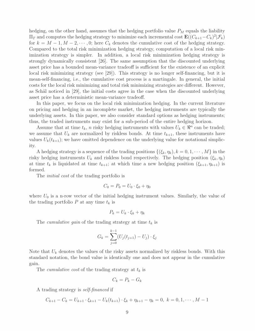
In this paper, we focus on the local risk minimization hedging. In the current literatureon pricing and hedging in an incomplete market, the hedging instruments are typically theunderlying assets. In this paper, we also consider standard options as hedging instruments;thus, the traded instruments may exist for a sub-period of the entire hedging horizon.

Assume that at time tk, n risky hedging instruments with values Uk ∈ n can be traded;we assume that Uk are normalized by riskless bonds. At time tk+1, these instruments havevalues Uk(tk+1); we have omitted dependence on the underlying value for notational simplic-ity.

A hedging strategy is a sequence of the trading positions (ξk, ηk), k = 0, 1, · · · , M in therisky hedging instruments Uk and riskless bond respectively. The hedging position (ξk, ηk)at time tk is liquidated at time tk+1; at which time a new hedging position (ξk+1, ηk+1) isformed.

The initial cost of the trading portfolio is

C0 = P0 = U0 · ξ0 + η0

where U0 is a n-row vector of the initial hedging instrument values. Similarly, the value ofthe trading portfolio P at any time tk is

Pk = Uk · ξk + ηk

The cumulative gain of the trading strategy at time tk is

Gk =

k−1∑j=0

(Uj(tj+1) − Uj) · ξj

Note that Uk denotes the values of the risky assets normalized by riskless bonds. With thisstandard notation, the bond value is identically one and does not appear in the cumulativegain.

The cumulative cost of the trading strategy at tk is

Ck = Pk − Gk

A trading strategy is self-financed if

Ck+1 − Ck = Uk+1 · ξk+1 − Uk(tk+1) · ξk + ηk+1 − ηk = 0, k = 0, 1, · · · , M − 1

9

When a market is incomplete, a risk minimization hedging strategy is fundamentallydifferent from hedging strategies based on risk adjusted option values, e.g., delta hedgingand semi-static hedging which is based on the principle of replicating a complex option withstandard options [8, 9]. Consider hedging a lookback option using the underlying as an ex-ample. Delta hedging, which is based on continuously rebalancing, is computed from thesensitivity of risk adjusted option values to the underlying. Thus delta hedging requires aprice dynamics under a risk adjusted measure which is typically obtained by calibration tothe standard option market. For hedging lookback options embedded in insurance benefits,there are potentially serious difficulties due to the requirement of market calibration to theoption market. Firstly, for risk management and hedging purposes, real world price dynam-ics models are needed. Such models are essential to accurately quantify risks, for example,in emerging cost analysis and calculating reserves. They are equally essential for hedgingstrategy computation and analysis. A model for the market price evolution (in contrast to arisk adjusted price dynamics) is needed, particularly when hedging is difficult due to marketincompleteness. Secondly, any parsimonious model inevitably leads to calibration errors.Thirdly, if standard options are used as hedging instruments, it is crucial for a model tocalibrate to the forward implied volatilities (due to the long maturity). Unfortunately, this isdifficult to accomplish. For risk minimization hedging, one typically assumes statistical mod-els for the market value of the underlying and the market values of the hedging instrumentsat trading times; risk adjusted liability values are not needed. It may be possible to estimatesuch a model from the historical observable prices of the underlying and hedging instruments.We further discuss this possibility of computing risk minimization hedging strategies usingstandard options by explicitly modeling implied volatilities in §5. Given a statistical modelfor both the underlying asset and hedging instruments, a risk minimization hedging strategyis computed to minimize hedge risk. Finally a risk minimization hedging achieves optimalityunder a chosen risk measure. For example, a local risk minimization hedging strategy isoptimal with respect to the specified trading requirement and the quadratic increment cost.Delta hedging and semi-static hedging are typically not optimal with respect to the discretetrading specification.

3 Hedging Using the Underlying Asset

In practice, hedging options embedded in the variable annuities is a risk management problemin an incomplete market. In our discussion so far, we have emphasized the theoreticaldifference between a risk minimization hedging strategy based on an incomplete marketassumption and a hedging strategy based on risk adjusted valuation. In this section, weevaluate, computationally, the effectiveness of delta hedging and risk minimization hedgingusing the underlying asset for a GMDB with a ratchet feature. As discussed in §2, the payoffof the option embedded in the variable annuity with a ratchet benefit can be expressed asΠT = max(HT − ST , 0) where the path dependent (ratchet) value HT = HtM

and

Hti = maxSt0 , St1 , St2 , · · · , Sti−1 = max(Hti−1

, Sti−1), 1 ≤ i ≤ M.

We evaluate hedging performance in terms of the total risk and total cost at the maturityT for the entire hedging horizon from t = 0 to T . Let P sf

M denote the time T self-financed

10

annually monthly biweeklyΠT RM delta ΠT RM delta ΠT RM delta

C0 0 18.1 20 0 19.8 20 0 19.9 20mean(ΠT − P sf

M) 24.4 0.387 -8.45 24 0.0638 -0.762 24.9 0.2 -0.186std(ΠT − P sf

M) 36.9 24 36.2 36.3 7.96 11.4 37.7 5.62 7.98√E((ΠT − P sf

M)2) 44.3 24 37.2 43.6 7.96 11.4 45.2 5.62 7.99mean(total cost) 24.4 30.2 24.5 24 32.7 32.2 24.9 33 32.8

VaR(95%) 95.2 40.7 45 94.8 12.5 16.6 97.6 9 12.1CVaR(95%) 136 63.9 73.9 134 19.5 26.4 140 13.8 18.9

#scenarios =20000 σ = 0.2 r = 0.05 µ = 0.1 T = 10

Table 1: Delta Hedging versus RM Hedging Using the Underlying (under a BS Model)

hedging portfolio value corresponding to a hedging strategy. For example, if (ξk, ηk), k =0, · · · , M −1 represents the optimal holdings computed from the risk minimization hedgingcomputation, then

P sfM = P0 + GM = U0 · ξ0 + η0 +

M−1∑j=0

(Uj(tj+1) − Uj) · ξj

The total risk ΠT −P sfM measures the amount of money that the hedging strategy is short

of meeting the liability at maturity T . The total cost ΠT −GM is the time T lookback optionpayoff plus the cumulative loss, −GM , of the hedging strategy. Unless stated otherwise, amaturity of ten years and a zero dividend yield are assumed in the computational results.

We compare the expected total cost and the first two moments of the total risk. Infor-mation about liability (payoff) at maturity T is listed under the column ΠT for comparison;it corresponds to no hedging. Results obtained using the underlying for biweekly hedging,monthly hedging, and annually hedging are given under the column biweekly, monthly, andannually respectively.

In addition, for a given confidence level, we report the Value-at-Risk (VaR) and theconditional Value-at-Risk (CVaR) of the total risk at the maturity T . For example, VaR(95%)is the minimum amount of money, that the self-financed hedging portfolio P sf

M is short ofmeeting the liability ΠT , with 5% probability; it is the cost at T , for the hedger, that isexceeded with 5% probability. The value CVaR(95%) is, with a 95% confidence level, theconditional expected cost that a hedging strategy requires at T , conditional on the cost isgreater than VaR(95%).

Although a Black-Scholes model is not adequate for modeling a return distribution witha fat tail, we first assume a Black-Scholes model and consider using the underlying as thehedging instrument; this is interesting since the market incompleteness in this case comesentirely from our inability to hedge continuously. Under a Black-Scholes model, the real

11

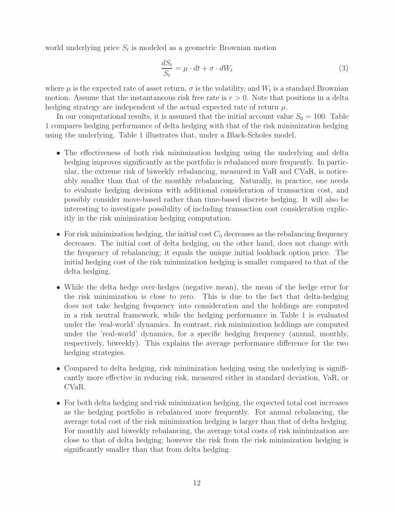
world underlying price St is modeled as a geometric Brownian motion

dSt

St= µ · dt + σ · dWt (3)

where µ is the expected rate of asset return, σ is the volatility, and Wt is a standard Brownianmotion. Assume that the instantaneous risk free rate is r > 0. Note that positions in a deltahedging strategy are independent of the actual expected rate of return µ.

In our computational results, it is assumed that the initial account value S0 = 100. Table1 compares hedging performance of delta hedging with that of the risk minimization hedgingusing the underlying. Table 1 illustrates that, under a Black-Scholes model,

• The effectiveness of both risk minimization hedging using the underlying and deltahedging improves significantly as the portfolio is rebalanced more frequently. In partic-ular, the extreme risk of biweekly rebalancing, measured in VaR and CVaR, is notice-ably smaller than that of the monthly rebalancing. Naturally, in practice, one needsto evaluate hedging decisions with additional consideration of transaction cost, andpossibly consider move-based rather than time-based discrete hedging. It will also beinteresting to investigate possibility of including transaction cost consideration explic-itly in the risk minimization hedging computation.

• For risk minimization hedging, the initial cost C0 decreases as the rebalancing frequencydecreases. The initial cost of delta hedging, on the other hand, does not change withthe frequency of rebalancing; it equals the unique initial lookback option price. Theinitial hedging cost of the risk minimization hedging is smaller compared to that of thedelta hedging.

• While the delta hedge over-hedges (negative mean), the mean of the hedge error forthe risk minimization is close to zero. This is due to the fact that delta-hedgingdoes not take hedging frequency into consideration and the holdings are computedin a risk neutral framework, while the hedging performance in Table 1 is evaluatedunder the ’real-world’ dynamics. In contrast, risk minimization holdings are computedunder the ’real-world’ dynamics, for a specific hedging frequency (annual, monthly,respectively, biweekly). This explains the average performance difference for the twohedging strategies.

• Compared to delta hedging, risk minimization hedging using the underlying is signifi-cantly more effective in reducing risk, measured either in standard deviation, VaR, orCVaR.

• For both delta hedging and risk minimization hedging, the expected total cost increasesas the hedging portfolio is rebalanced more frequently. For annual rebalancing, theaverage total cost of the risk minimization hedging is larger than that of delta hedging.For monthly and biweekly rebalancing, the average total costs of risk minimization areclose to that of delta hedging; however the risk from the risk minimization hedging issignificantly smaller than that from delta hedging.

12

Table 1 clearly indicates that, under a Black-Scholes model, risk minimization hedgingusing the underlying is better than delta hedging since the former minimizes risk under theassumption that hedging portfolio is rebalanced at the specified times.

Unfortunately, a Black-Scholes model (3) is not appropriate for the risk managementof variable annuities since the embedded options are sensitive to tails of the underlyingdistribution; we consider the Black-Scholes model here to illustrate the difference betweenrisk minimization hedging using the underlying and delta hedging when the incompletenesscomes from discrete rebalancing, not additional risks such as jump or volatility. Determininga suitable model for the underlying is usually a challenging task; it is even more difficult forvariable annuities due to the long maturities and sensitivities of the payoff to the extremeprice movements. The Canadian Insurance Association on Segregated Funds (SFTF) recom-mends that model calibration be adjusted to give a sufficiently accurate fit in the left tailof the distribution [17]. A Black-Scholes model certainly seems a poor choice in this regard.Next we consider Merton’s jump diffusion model which is more suitable to model fat tails ofreturn distributions.

Let us assume that the real world price dynamics is modeled by a jump diffusion modelwith a constant volatility, i.e.,

dSt

St= (µ − q − κλ) · dt + σ · dWt + (J − 1) · dπt (4)

where r is the risk free rate, q is the continuous dividend yield, and σ is a constant volatility.In addition, πt is a Poisson counting process, λ > 0 is the jump intensity, and J is a randomvariable of jump amplitude with κ = E(J − 1). For simplicity, log J is assumed here to be

normally distributed with a constant mean µJ and variance σ2J ; thus E(J) = eµJ+ 1

2σ2

J .While a risk minimization hedging strategy is computed directly from the original process

(4), delta hedging is computed from a risk adjusted value of the option. When jump riskexists, no arbitrage option value is no longer unique. Thus a delta hedging strategy and itsassociated hedging cost depends on how the risk is adjusted from the real world price process(4).

From the utility-based equilibrium theory, assuming γ ≤ 1 is the risk aversion parameter,a risk-adjusted price process corresponding to (4) is [23]

dSt

St= (r − q − κQλQ) · dt + σ · dW Q

t + (JQ − 1) · dπQt (5)

where W Qt is a standard Brownian motion and πQ

t is a Poisson counting process and log JQ

is normally distributed with

σQJ = σJ

µQJ = µJ − (1 − γ)σ2

J

λQ = λe−(1−γ)(µJ− 12(1−γ)σ2

J )

where κQ = E(JQ − 1). As an investor becomes more risk averse, the jump frequency andthe expected magnitude of jumpsize are adjusted to larger quantities. In other words, theoptions are priced according to a larger (combined diffusion and jump) risk.

13

Our objective is to compute a hedging strategy under the assumption that a real worldprice dynamics (4) is given. To determine a delta hedge one needs to first choose a risk aver-sion parameter and then evaluate the risk adjusted lookback option values V (S, t). Choosinga risk aversion parameter is ad-hoc in nature and much effort has been spent by economists tofind appropriate risk aversion parameters. Alternatively, one can calibrate with the currentmarket standard option prices to determine a risk adjusted process from these prices.

Under a Merton’s jump model (5), analytic formula exists for density functions [22] andstandard option pricing. Assume that currently t = 0 and q(x) is a probability densityfunction for x = log ST under (4). From [23], the characteristic function for x is

φq(z) =

∫ ∞

−∞q(x)eizxdx = eizωT−z2T σ2

2+(eizµJ− 1

2 z2σ2J−1)λT

where

ω = µ − q − σ2

2− λκ.

Hence the PDE for a Merton’s jump model is given by

q(x) =1

2π

∫ ∞

−∞φq(z)e−izxdz

It can be easily shown that [22]

q(x) =e−λT

√2π

⎛⎜⎝

∞∑n=0

(λT )n

n!· e

− (ωT+nµJ−x)2

2(Tσ2+nσ2J

)√Tσ2 + nσ2

J

⎞⎟⎠

For computational results in this paper, analytic formula for transitional density functionsunder a Merton’s jump diffusion model (or Black-Scholes model) are used to compute deltahedging strategies and risk minimization hedging strategies. For delta hedging, the analyticformula for the transitional density function is used to compute values of lookback optionsbased on (2). For risk minimization hedging strategies, analytic formula for the transitionaldensity function and standard option values are used to compute optimal hedging positions ona finite grid; the hedging strategies corresponding to independent simulations are computedusing spline interpolations from the hedging positions on the grid.

When the risk aversion parameter γ = 1, options are priced risk neutrally; the investorsprice the asset under the risk free interest rate. In our example, we assume that the jumpfrequency λ = 20%, i.e., approximately a jump once every 5 years on average, a mean of−30% and a volatility of 15% for the logarithm of the jumpsize. Table 2 compares, underthe risk neutral assumption, the effectiveness of delta hedging with the risk minimizationhedging using the underlying. From Table 2, it can be observed that

• Both hedging strategies are more effective as one rebalances more frequently. How-ever, due to jump risk, the improvement of more frequent rebalancing is less dramaticcompared to that under the Black-Scholes model. Specifically, compared to annualrebalancing, monthly or biweekly rebalancing, under a Merton’s jump diffusion model,improves the hedging performance only slightly further.

14

annually monthly biweeklyΠT RM delta ΠT RM delta ΠT RM delta

C0 0 22.7 20.8 0 24.3 20.8 0 24.4 20.8mean(ΠT − P sf

M) 27.9 0.427 -7.77 27.4 0.042 -0.746 28.2 0.0777 -0.274std(ΠT − P sf

M) 43.6 28.5 44.9 43.5 20.8 27.4 45.3 19.7 25.7√E((ΠT − P sf

M)2) 51.7 28.5 45.5 51.4 20.8 27.4 53.4 19.7 25.7mean(total cost) 27.9 37.8 26.6 27.4 40.1 33.6 28.2 40.2 34.1

VaR(95%) 116 49.9 62.4 115 35.3 44.9 120 33.7 42.6CVaR(95%) 162 77.8 97.8 162 54.9 68.9 169 51.4 64.5

MJD Model: #scenarios = 20000 σ = 0.15 r = 0.05 µ = 0.1 T = 10risk aversion γ = 1 λ = 0.2 µJ = −0.3 σJ = 0.15

Table 2: Delta Hedging versus RM Hedging Using the Underlying (under a MJD Model)

• Compared to delta hedging, risk minimization hedging using the underlying is signifi-cantly more effective in reducing risk under a jump diffusion model. Not surprisingly,risk minimization hedging incurs a larger average cost.

• For annual rebalancing, delta hedging can perform worse than not hedging at all asmeasured by the standard deviation of hedging error.

• The monthly risk minimization hedging using the underlying significantly reduces therisk, relative to an un-hedged position.

If delta hedging is determined from a risk adjusted model which is calibrated from theoption market and has a risk aversion parameter γ < 1, the option is not priced risk neutrally.Thus the delta hedging strategy depends on how the option market or the hedger adjuststhe jump risk; risk minimization hedging, on the other hand, is typically determined undera probability measure for the market price dynamics.

4 Hedging Using Standard Options

With the rapid growth of derivative markets, it is now a common practice in the financialindustry to use liquid vanilla options to hedge an exotic option. The S&P 500 index optionstraded on the exchange, for example, are natural instruments for hedging variable annuitieswith guarantees linked directly to or highly correlated to the S&P 500 index.

In this section, we assume that there is no transaction cost and compare risk minimizationhedging using the underlying with risk minimization hedging using standard options underthe Black-Scholes model as well as Merton’s jump model; we discuss volatility risks in thenext section.

To illustrate, we assume that hedging instruments are standard options with one yearmaturity; liquid options with a shorter maturity can similarly be used. We consider hedg-ing using 6 options, 3 calls with strikes [100%, 110%, 120%] · St and 3 puts with strikes

15

ΠT monthly annually annually annuallyunderlying underlying option(6) option(2)

C0 0 17.3 13.9 17.7 17.4mean(ΠT − P sf

M) 11.4 0.0766 0.326 0.00956 -0.0927std(ΠT − P sf

M) 20.9 5.46 15.9 1.6 4.61√E((ΠT − P sf

M)2) 23.8 5.47 15.9 1.6 4.61mean(total cost) 11.4 23.5 19.1 23.9 23.4

VaR (95%) 55.4 8.91 28.5 2.42 7.02CVaR (95%) 77.3 13 43.2 3.81 11.9

BS Model: #scenarios = 20000 σ = 0.15 r = 0.03 q = 0 µ = 0.1 T = 10

Table 3: RM Hedging Using the Underlying versus RM hedging Using Options (a BS Model)

[80%, 90%, 100%] · St, and hedging using 2 at-the-money options (one call and one put withstrike equal the current underlying value).

Table 3 compares, under a Black-Scholes model, monthly and annually rebalancing usingthe underlying with annual rebalancing using 6 options and 2 options respectively. Table 4presents a similar comparison but under a Merton’s jump diffusion model (4).

Table 3 and Table 4 illustrate that, compared to hedging using the underlying, optionhedging leads to better risk reduction. More specifically,

• Under a Black-Scholes model, monthly rebalancing using the underlying and annualrebalancing using two options have similar initial costs and average total costs. How-ever, better risk reduction (measured either in standard deviation, VaR, or CVaR ofthe total risk) is achieved using two options compared to monthly hedging using theunderlying. In addition, compared to hedging using 2 options, hedging using 6 optionsincurs slightly larger initial and average total costs but achieves significantly better riskreduction.

• Under a Merton’s jump model, hedging using 6 options incurs slightly more initial andaverage total costs than hedging using 2 options. However, hedging using 6 optionsachieves better risk reduction than hedging using 2 options: contrast a CVaR(95%)value of 4.61 using 6 options with a CVaR(95%) value of 15.2 using 2 options. Inaddition, hedging using 2 options is much better than monthly rebalancing using theunderlying in risk reduction; the initial cost and average total cost of option hedgingis larger than that of hedging using the underlying. This result suggests that, in thepresence of jump risk, option hedging leads to better risk reduction even though it mayincur slightly larger costs.

5 Hedging Under Volatility Risks

Computational results in §4 clearly suggest that standard options have potential use inhedging risks embedded in variable annuities. Specifically, Table 3 and 4 suggest that,

16

ΠT monthly annually options(6) options(2)C0 0 22.8 19.5 25.2 24.6

mean(ΠT − P sfM) 16.4 0.123 0.445 0.0159 -0.0884

std(ΠT − P sfM) 28.8 13 21.4 1.85 6√

E((ΠT − P sfM)2) 33.1 13 21.4 1.85 6

mean(totalCost) 16.4 30.9 26.8 34 33.1VaR (95%) 75 23.5 38.4 2.75 8.4

CVaR (95%) 108 38.4 60.5 4.61 15.2

MJD Model: #scenarios = 20000 σ = 0.15 r = 0.03 µ = 0.1 T = 10q = 0 γ = −1.5 λ = 0.1 µJ = −0.2 σJ = 0.15

Table 4: RM Hedging Using the underlying versus Using Options (a MJD Model)

hedging using standard options produces significantly greater risk reduction than using theunderlying, particularly under a jump diffusion model.

Does this imply that one should hedge using options? To make this decision, we needto evaluate hedging strategies under more realistic market price evolution assumptions. Inparticular, when standard options are used as hedging instruments, quantifying risk andhedging performance depends on accurately modeling the market option price dynamics, inaddition to the underlying dynamics. Moreover, one needs to consider other factors suchas transaction costs, liquidity risk, and default risk. In this section, we focus on evaluatinghedging effectiveness under more realistic market price models which account for impliedvolatility risks.

Given the current market convention of quoting implied volatilities instead of optionprices, accurately modeling evolution of market implied volatilities is necessary. Followingmarket practice, implied volatility here is defined by inverting the Black-Scholes formulafrom an option price.

Implied volatilities have been observed to display a curvature across moneyness and aterm structure across time to maturity. In addition to modeling this static implied volatilitystructure, the evolution of the implied volatilities over time needs to be accurately modeledwhen standard options are used as hedging instruments. There has been active research inrecent years on the evolution of the market implied volatilities over time based on historicimplied volatility data, e.g., [13, 15, 35]. Zu and Avellaneda [35] construct a statisticalmodel for the term structure of the implied volatilities for currency options. Cont et al[13] observe that, for major indices including S&P 500, the implied volatility surface changesdynamically over time in a way that is not taken into account by current modeling approaches,giving rise to ”Vega” risk in option portfolios. They believe that option markets may havebecome increasingly autonomous and option prices are driven, in addition to movements inthe underlying, also by internal supply and demand in the options market. They study theimplied volatility time series for major indices, including S&P500 from March 2, 2002 andFebruary 2, 2003, and observe that:

• Implied volatilities are not static; they fluctuate around their means. The daily stan-dard deviation of the implied volatility can be as large as a third of its typical value

17

for out-of-the money options.

• The variance of daily log-variations in the implied volatility surface can be satisfactorilyexplained in terms of two or three principal components.

• The first principal component reflects an overall shift in the level of all implied volatil-ities which accounts for around 80% of the daily variance [13]. The second principalcomponent explains the opposite movement of the out-of-the-money call and put im-plied volatilities while the third principal component reflects change in the convexityof the volatility surface. In addition, there is a strong negative correlation between theindex return and the change of the implied volatility level; the correlations betweenthe underlying return and the other components of implied volatility changes are eithersignificantly smaller or negligible.

Hence, in order to accurately quantify the hedging effectiveness when the hedging in-struments consist of standard options, implied volatility risk needs to be suitably modeled.Unfortunately, under both the Black-Scholes model and Merton’s jump diffusion model, im-plied volatilities are constant over time. This clearly is a substantial departure from theobserved dynamics of the market implied volatilities.

How should the dynamics of the implied volatilities be modeled? To hedge a derivativecontract, the typical approach is to assume a model for the underlying price evolution andderive implied volatilities from the assumed underlying price model; an underlying model canbe estimated through calibration to the option market. Since both the Black-Scholes modeland Merton’s jump model lead to a static volatility surface, they are inadequate in modelingthe observed stochastic implied volatilities. Amongst the typical models for underlying prices,only a stochastic instantaneous volatility underlying model can generate stochastic impliedvolatilities.

Unfortunately, the fact that instantaneous volatility is not directly observable presentsmany challenges for hedging and model estimation under an instantaneous volatility model.

• Firstly, it is difficult to adjust hedging positions according to an unobservable value.

• Secondly, it is not clear how to estimate an instantaneous volatility price model, fromhistorical data, given that the instantaneous volatility is not observable; a stochasticinstantaneous volatility underlying model can only be calibrated from liquid optionprices. Moreover, the model obtained by calibrating to the market option prices givesthe price model under a risk adjusted measure. As previously discussed, for hedgingand risk management assessment we need a model for the real world market pricedynamics.

• Thirdly it is difficult to calibrate the current market option prices sufficiently accu-rately using a parsimonious stochastic volatility model with a small number of modelparameters, e.g., Hestons model [20]. In addition, there is no evidence that such astochastic volatility model for the underlying is capable of modeling the evolution ofthe implied volatilities over time.

• Fourthly, even if a model calibrates the market prices by allowing a sufficient numberof model parameters, e.g., a jump diffusion model with a local volatility function [2], it

18

is difficult to accurately model the implied volatility evolution for a long time horizonbased on market calibration. A model that sufficiently calibrates the market impliedvolatilities today may give a poor fit for the implied volatilities tomorrow. This can beproblematic for hedging and risk management purposes.

In addition to the cautionary remarks provided above, there are also arguments aboutwhether an option pricing model derived from any underlying price model can adequatelymodel option price evolution because of the autonomy of option market, e.g., [13]. Thissuggests that it is reasonable and possibly better to consider a joint model for the underlyingprice and implied volatility evolutions.

In [31], Schonbucher jointly models, under a risk adjusted measure, the underlying andimplied volatility evolution in which the instantaneous volatility and implied volatility bothbecome state variables. No arbitrage restriction is established for the joint processes undera risk adjusted measure.

Since our focus is risk management and hedging for options embedded in variable annu-ities, we are interested in modeling the real world price evolution for both the underlying andhedging options. To evaluate hedging effectiveness of discrete dynamic hedging strategies forvariable annuities, a joint discrete time model for real-world underlying and hedging instru-ment price changes between each rebalancing time is needed. In particular, this model needsto accurately describe the tails of the underlying price distribution and (mean reverting)stochastic implied volatility dynamics.

More specifically, we are interested in modeling the most liquid implied volatilities. Weassume that the time to maturity of the option hedging instruments is fixed at one year (ashorter maturity can similarly be used) and far out-of-the money options are not used ashedging instruments due to liquidity considerations. Since change in the implied volatilitylevel explains 80% of the daily variation in implied volatilities, as a first improvement, wemodel the at-the-money implied volatility evolution and assume that the ratios of impliedvolatilities to the at-the-money implied volatility are constant over time.

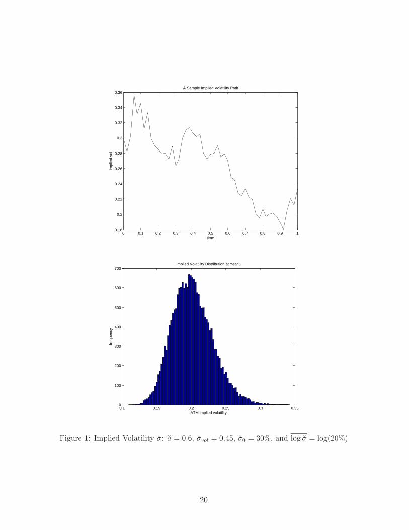
Let σt denote the at-the-money implied volatility with a time to maturity of one year.Using an Ornstein-Uhlenbeck process, this at-the-money implied volatility σt is modeled asfollows

d log(σt) = a · (log σ − log(σt)) · dt + σvol · dZt (6)

where Zt is a standard Brownian, log σ denotes the long term average value (of the logarithmof the at-the-money implied volatility level). Figure 1 displays a sample path and distributionof the implied volatility σt at time t = 1 year under the assumed model parameters; this modelis used for at-the-money implied volatility in our subsequent computational investigation.

It is important to note that, by modeling implied volatilities directly, the standard optionprices are directly given by the implied volatilities via the Black-Scholes formula; theseliquid option values are no longer determined by the underlying price model. There are manyadvantages gained by computing a risk minimization hedging using standard options based ona model with implied volatilities directly as state variables. Firstly, the implied volatilities aredirectly observable from the market. This makes it possible to estimate a model from historicdata and adjust hedging positions based on the implied volatilities. Secondly, by modelingthe market implied volatility directly, calibration to market is automatically accomplished

19

0 0.1 0.2 0.3 0.4 0.5 0.6 0.7 0.8 0.9 10.18

0.2

0.22

0.24

0.26

0.28

0.3

0.32

0.34

0.36

time

impl

ied

vol

A Sample Implied Volatility Path

0.1 0.15 0.2 0.25 0.3 0.350

100

200

300

400

500

600

700

ATM implied volatility

freq

uenc

y

Implied Volatility Distribution at Year 1

Figure 1: Implied Volatility σ: a = 0.6, σvol = 0.45, σ0 = 30%, and log σ = log(20%)

20

by setting the initial implied volatilities to the market implied volatilities. Thirdly, thehedging instruments are valued exactly using the Black-Scholes formula according to themarket practice. For simplicity, we have modeled here only change in the level of the impliedvolatilities; but the approach can be extended (with additional computational complexity)to model the opposite movement of the implied volatilities for out-of-the money calls andputs and change in the convexity of the implied volatility curve.

Since the instantaneous volatility is not directly observable in practice, it is difficult toestimate a model with an instantaneous volatility as a state variable and adjust hedgingpositions based on this unobservable variable. Thus, when computing hedging strategies, weonly assume a crude (constant) approximation σ0 of the instantaneous volatility (for exampleσ0 can be an estimation of the average of the instantaneous volatility over time). In otherwords, we compute risk minimization option hedging strategies under the joint model (7)below for the underlying price and the implied volatility σt:

dSt

St= (µ − q − κλ) · dt + σ0 · dWt + (J − 1) · dπt

d log(σt) = a · (log σ − log(σt)) · dt + σvol · dZt,(7)

where Wt and Zt can be correlated in general. Note that the approach of determining optionprices by modeling the underlying price evolution as described in §3 and §4 can be consideredas a special case of a model (7) with a = σvol = 0. In addition, jumps can be introduced inthe mean reverting implied volatility dynamics as well.

Presently, for computational simplicity, we compute hedging strategies based on a jointmodel (7) assuming that Wt and Zt are independent. However, we evaluate hedging effec-tiveness under a joint model with both instantaneous volatility risk and implied volatility risk,and possibly correlation between these risks. Specifically, we evaluate hedging performanceunder the joint price model (8) below:⎧⎨

⎩dSt

St= (µ − q − κλ) · dt + σt · dWt + (J − 1) · dπt

d log(σt) = a · (log σ − log(σt)) · dt + σvol · dXt

d log(σt) = a · (log σ − log(σt)) · dt + σvol · dZt,

(8)

where log σ denotes the long term average value (of the logarithm of the instantaneousvolatility), and Wt, Xt, and Zt can be correlated. Evaluating hedging effectiveness under thisjoint dynamics provides an assessment of the impact of ignoring correlation and instantaneousvolatility risk in the hedging strategy computation.

We now compare effectiveness of the risk minimization hedging using the underlying withrisk minimization hedging using six standard options. In addition to monthly hedging usingthe underlying, we compare the option hedging strategy computed by explicitly modeling theimplied volatility risk in the risk minimization hedging computation (under column option(6)-σ) with the risk minimization option hedging strategy for which the hedging positions at timetk are computed assuming that the implied volatility remains at the time tk level from tk to thematurity T (under column option(6)-reset); this is similar to computing a hedging strategyby recalibrating implied volatilities. We note that the risk minimization hedging option(6)-σcomputes holdings on a 3-dimensional grid, along the directions of the underlying, runningmax, and at-the-money implied volatility.

Tables 5 & 6 compare the hedging performance of these three strategies. In these com-putations, the initial implied volatilities are set to the Black-Scholes implied volatilities cor-

21

responding to the option prices computed under the underlying dynamics in the model (7);parameters for the model (7) are a = a = 0.6, log σ = log σ = log(20%), with other parame-ters given explicitly in the table. The only difference in computational setup between Table5 and Table 6 is that the constant volatility σ0 in the model (7) is set to different values;thus the initial implied volatilities σ0 are different as well. From Table 5 & 6, we observe thefollowing:

• Hedging using the underlying is sensitive to instantaneous volatility risk which is dif-ficult to model; this is indicated by the different costs and risks under the columnunderlying-σ in Table 5 & 6. In Table 5, hedging using the underlying leads to anunder hedge of the payoff since a constant volatility of 15%, which is lower than theaverage of 20%, is used in the hedging computation. In Table 6, hedging using theunderlying leads to an over hedge since a constant volatility of 22%, higher than theaverage of 20%, is used in the hedging computation.

• For hedging strategy option(6)-reset computed by resetting the implied volatility levelat time tk to σtk from tk to the maturity T , the hedging strategy and its performance issimilarly sensitive to the initial implied volatility level. For example, hedging strategyoption(6)-reset under-estimates the initial hedging cost in Table 5, while the initialhedging cost is over-estimated in Table 6.

• When the implied volatility σt is explicitly modeled in the risk minimization hedgingframework, column option(6)-σ, the hedging strategy computation takes the future im-plied volatility dynamics into consideration and the initial hedging cost is significantlyless sensitive to the initial implied volatility level; note the striking similarities of theperformance assessment under the column option(6)-σ for Table 5 & 6. Moreover, wenote that, compared to hedging using the underlying, hedging using options remainssignificantly more effective in risk reduction under both jump and volatility risks.

Table 7 displays the hedging performance when there is no instantaneous volatility risk(instantaneous volatility is a constant). We emphasize that the implied volatility evolutionis modeled in the option hedging strategy option(6)-σ. Comparing Table 7 with Table 5, thehedging results indicate sensitivities to the instantaneous volatility risk. It can be observedthat hedging effectiveness of the risk minimization hedging using options under the impliedvolatility model (corresponding to the hedging strategy option(6)-σ) is relatively insensitiveto instantaneous volatility risk. This suggests that hedging using standard options may po-tentially be an effective way of reducing instantaneous volatility risk, when implied volatilityrisk is properly modeled. Hedging using the underlying, on the other hand, is sensitive tothe instantaneous volatility risk.

Table 5 and Table 6 indicate that hedging using options by simply resetting the impliedvolatility level at the rebalancing time, i.e., option(6)-reset, either over- or under- estimatesthe initial hedging costs. Figure 2 display the relative frequency (frequency divided by thenumber of simulations) of the increment cost (Uk+1ξk+1 + ηk+1)− (Uk(tk+1)ξk + ηk). The topplot displays the relative frequency of the incremental cost for the hedging strategy option(6)-σ computed by explicitly modeling the implied volatility evolution; the bottom plot is forthe hedging strategy option(6)-reset which simply assumes that the future implied volatilitystays at the current level at each rebalancing time. The hedging strategy, option(6)-reset,

22

ΠσT monthly annually annually

underlying-σ option(6)-reset option(6)-σC0 0 23.7 21.5 28.8

mean(ΠT − P sfM) 31.4 20.5 10.8 0.612

std(ΠT − P sfM) 46.4 18.8 8.1 6.78√

E(ΠT − P sfM)2 56.1 27.8 13.5 6.81

mean(total cost) 31.4 52.5 39.9 39.4VaR (95%) 118 54.4 24.3 11.4

CVaR (95%) 174 76.8 31.5 18.6

MJD Model: #scenarios = 20000 σ0 = 0.15 r = 0.03 T = 10 α = 0.1λ = 0.12 µJ = −0.2 σJ = 0.15 γ = 1

Table 5: Hedging Comparison Under a Volatility Model (8) : σvol= 0.45 , σvol= 0.45


underlying-σ option(6)-reset option(6)-σC0 0 35.6 35 28.9

mean(ΠT − P sfM) 31.5 -6.26 -8.65 0.374

std(ΠT − P sfM) 46.7 15.6 7.72 6.48√

E(ΠT − P sfM)2 56.3 16.8 11.6 6.49


CVaR (95%) 175 33.9 8.64 16.8

MJD Model: #scenarios = 20000 σ0 = 0.22 r = 0.03 q = 0 T = 10α = 0.1 λ = 0.12 µJ = −0.2 σJ = 0.15 γ = 1

Table 6: Hedging Comparison Under a Volatility Model (8): σvol= 0.45 , σvol= 0.45



mean(ΠT − P sfM) 17.7 0.583 10.8 0.627

std(ΠT − P sfM) 30.8 13.9 6.25 5.71√

E(ΠT − P sfM)2 35.5 13.9 12.5 5.74

mean(total cost) 17.7 32.5 39.9 39.4VaR (95%) 80.4 25.1 21.5 10.2

CVaR (95%) 116 40.7 26 14.8


Table 7: Hedging Comparison Under a Volatility Model (8): σvol= 0 , σvol= 0.45

23



mean(ΠT − P sfM) 31.4 20.5 10.1 -0.401

std(ΠT − P sfM) 46.4 18.8 7.89 6.5√

E(ΠT − P sfM)2 56.1 27.8 12.8 6.51


CVaR (95%) 174 76.8 29.8 14.6


Table 8: Hedging Comparison Under a Volatility Model (8): corr(Zt, Wt) = −.6, σvol= 0.45,σvol= 0.45

leads to a significantly larger average and variance of the incremental cost at each rebalancingtime compared to the risk minimization hedging option(6)-σ for which the implied volatilityrisk is properly modeled.

Finally, Table 8 illustrates the hedging effectiveness of the three strategies evaluatedunder a correlation assumption between the change in log σt and the Brownian innovationof the asset return, specifically corr(Wt, Zt) = −0.6 in the model (8). Comparing Table8 with Table 5, it can be observed that hedging effectiveness using standard options is notsignificantly affected by the correlation risk in terms of the standard deviation of the hedgingerror. However, VaR and CVaR become slightly smaller for this example.

6 Concluding Remarks

Accurate quantification and robust hedging of the market risk embedded in a guaranteedminimum death benefit of a variable annuity contract is a new and challenging task forthe insurance industry. This is mainly due to the exposure to the equity market risk, longmaturity of the insurance contract, and the sensitivity of the benefit to the tails of theaccount value distribution. For this type of contracts, risk quantification and risk reductionrequire accurately modeling of the evolution of both the underlying account value and hedginginstrument prices. In addition to a good model, effectiveness of a hedging strategy dependson the method from which hedging positions are determined. A delta hedging strategy iscomputed based on option values under a risk adjusted measure. A risk minimization hedgingstrategy is computed to minimize risk based on a model for the real world price evolution andrebalancing specification. We analyze and compare these different hedging methods usingeither the underlying or standard options to hedge a lookback option embedded in variableannuity contracts for which the minimum death guarantee has a ratchet feature.

Due to sensitivity of such a variable annuity benefit to the tails of the account value dis-tribution, jump risk and volatility risks need to be appropriately modeled. These additionalrisks, and the fact that dynamic hedging can only be implemented at discrete times with a

24

1 2 3 4 5 6 7 8 9 10 11−50

0

50

100

150

200

relative frequency at each rebalancing time

incr

emen

tal c

osts

Model ATM Implied Volatility

1 2 3 4 5 6 7 8 9 10 11−150

−100

−50

0

50

100

150

200

relative frequency at each rebalancing time

incr

emen

tal c

osts

Reset ATM Implied Volatility


Figure 2: Incremental Costs Under a Volatility Model (8): σvol= 0.45, σvol= 0.45, σ0= 0.15

25

limited choice of hedging instruments, suggest that hedging options embedded in variableannuities are hedging problems in an incomplete market. Thus it may be more appropriateto compute a hedging strategy to directly minimize a measure of the hedge risk given a setof trading times and a set of hedging instruments; this is the risk minimization hedging.

We evaluate and compare effectiveness of delta hedging with risk minimization hedgingusing the underlying under a Black-Scholes model as well as a Merton’s jump diffusionmodel. We first assume that there is no volatility risk and illustrate that risk minimizationhedging using the underlying is superior to delta hedging. In addition, monthly rebalancingrisk minimization hedging using the underlying is relatively effective under a Black-Scholesmodel; the hedging effectiveness further improves as hedging portfolio is rebalanced morefrequently. Moreover, under a Merton’s jump model, risk reduction in both delta hedgingand risk minimization hedging using the underlying is less effective. In particular, for bothmethods, improvement of biweekly hedging over monthly hedging is less significant.

Due to the increasing liquidity of standard options, we compare risk minimization hedgingusing standard options to that of using the underlying. We observe that the risk minimizationhedging using standard options (even with only two at-the-money options) is significantlymore effective than that of using the underlying, particularly when jump risk is considered.

Maturities of variable annuities are usually long; this makes modeling of relevant risksespecially challenging. For hedging a long term derivative, volatility risk clearly cannotbe ignored. Hedging using the underlying asset is susceptible to instantaneous volatilityrisk. When standard options are used as hedging instruments, hedging effectiveness needsto be evaluated under the implied volatility risk. Since the instantaneous volatility is notdirectly observable, it is difficult to model instantaneous volatility risk and implement hedgingstrategies which adjust hedging positions according to this unobservable variable. The typicalapproach of calibrating a model for the underlying evolution from the option prices is facedwith the need for a complex model to match the current option prices and the need for aparsimonious model to stably model future option prices evolution. Moreover, the underlyingprice dynamics calibrated to the option market is under a risk adjusted measure rather thanthe real price dynamics necessary for risk quantification and hedging.

We compute a risk minimization hedging using standard options by explicitly modelingevolutions in the underlying as well as the at-the-money implied volatility. In our current in-vestigation, the ratios of the implied volatilities of hedging instruments to the at-the-moneyimplied volatility is assumed to be constant over time for simplicity. Since instantaneousvolatility is not observable, we compute hedging strategy assuming a constant approxima-tion to the instantaneous volatility in a model (7). By evaluating hedging performanceunder a joint model (8) of the underlying account value evolution, which includes instan-taneous volatility risk, and implied volatilities, we illustrate that, when implied volatilityrisk is suitably modeled, risk minimization hedging using standard options is effective inreducing lookback option risk embedded in variable annuity with a ratchet guaranteed min-imum death benefit. In particular, unlike hedging using the underlying, which yields largerhedging error due to failure to model instantaneous volatility risk, effectiveness of the riskminimization hedging using standard options is relatively insensitive to the presence of in-stantaneous volatility risk. We also illustrate hedging performance when the change of theimplied volatility is correlated to the change of the underlying.

Hedging variable annuities is a complex and challenging task. Investigation and analysis in

26

this paper are based on models which have been used to describe evolution of asset price withfat tails in the return distribution. For future investigation, it is important to evaluate howwell a joint model (8) for the underlying and implied volatility can describe, in practice, theunderlying market price and implied volatility evolution for a long time horizon. In additionto jump risk, volatility risks, other risks such as mortality risk, basis risk, and surrender riskalso need to be properly analyzed. In a separate paper [10], we analyze sensitivity of riskminimization hedging to interest risk and compute the optimal risk minimization hedgingstrategy under both equity and interest risks.

References

[1] K. Aase and S. Persson. Pricing of unit-linked life insurance policies. ScandianavianActuarial Journal, 1:26–52, 1994.

[2] L. Andersen and J. Andreasen. Jump-diffusion processes: Volatility smile fitting andnumerical methods for option pricing. Review of Derivative Research, 4:231–262, 2000.

[3] A. Bacinello and S. Perssen. Design and pricing of equity-linked life insurance understochastic interest rates. Journal of Risk Finance, 3:6–21, 2002.

[4] D. Bertsimas, L. Kogan, and A. Lo. Hedging derivative securities and incomplete mar-kets: An ε-arbitrage approach. Operations Research, 49:372–397, 2001.

[5] P. Boyle and M. Hardy. Reserving for maturity guarantees: Two approaches. Insurance:Mathematics and Economics, 21:113–127, 1997.

[6] P. Boyle and E. Schwartz. Equilibrium prices of guarantees under equity-linked con-tracts. Journal of Risks and Insurance, 44:639–680, 1977.

[7] M. Brennan and E. Schwartz. The pricing of equity-linked life insurance polcies withan asset value guarantee. Journal of Financial Economics, 3:195–213, 1976.

[8] Peter Carr. Semi-static hedging. Technical Report February, Courant Institute, NYU,2002.

[9] Peter Carr and Liuren Wu. Static hedging of standard options. Technical report, CourantInstitute, New York University, November 26, 2002.

[10] T. F. Coleman, Y. Li, and M. Patron. Hedging guarantees in variable annuities using riskminimization (under both equity and interest risks). Technical Report in preparation,Cornell University, 2004.

[11] T. F. Coleman, Y. Li, and M. Patron. Total risk minimization using Monte-carlo simu-lations. Technical Report in preparation, Cornell University, 2004.

[12] Thomas F. Coleman, Yuying Li, and M. Patron. Discrete hedging under piecewise linearrisk minimization. The Journal of Risk, 5:39–65, 2003.

27

[13] R. Cont and J. D. Fonseca. Dynamics of implied volatility surfaces. Quantative Finance,2:45–60, 2002.

[14] D. Duffie and H. R. Richardson. Mean-variance hedging in continuous time. Ann.Applied Probab., pages 1–15, 1991.

[15] M. Fengler, W. Hardle, and C. Villa. The dynamics of implied volatilities: a commonprincipal component approach. review of Derivative Research, 6, 2003.

[16] H. Follmer and M. Schweizer. Hedging by sequential regression: An introduction to themathematics of option trading. The ASTIN Bulletin, 1:147–160, 1989.

[17] M. Hardy. Investment Guarantees: Modeling and risk management for equity-linked lifeinsurance. John Wiley & Sons, Inc., 2003.

[18] D. Heath, E. Platen, and M. Schweizer. A comparison of two quadratic approaches tohedging in incomplete markets. Mathematical Finance, 11:385–413, 2001a.

[19] D. Heath, E. Platen, and M. Schweizer. Numerical comparison of local risk-minimisationand mean-variance hedging. In Option pricing, interest rates and risk management,pages 509–537. (ed. E. Jouini, J. Cvitanic and, M. Musiela), Cambridge Univ. Press,2001b.

[20] S.L. Heston. A closed-form solution for options with stochastic volatility with applica-tions to bond and currency options. Review of Financial Studies, 6:327–343, 1993.

[21] T.E. Hill. Variable annuity with guaranteed benefits, risk-based capital c-3 phase ii.Technical Report Novmeber, Milliman USA Research Report, 2003.

[22] G. Labahn. Closed form PDF for Merton’s jump diffusion model. Technical report,School of Computer Science, Unviersity of Waterloo, Waterloo, Ont., Canada N2L 3G1,2003.

[23] A. Lewis. Fear of jumps. Wilmott Magazine, December:60–67, 2002.

[24] A.G. Longley-Cook and J. Kehrberg. Efficient stochastic modeling utilizing represen-tative scenarios: Application to equity risks. Technical Report May, Milliman USAResearch Report, 2003.

[25] F. Mercurio and T. C. F. Vorst. Option pricing with hedging at fixed trading dates.Applied Mathematical Science, 3:135–158, 1996.

[26] F. Mercurio and T. C. F. Vorst. Option pricing with hedging at fixed trading dates.Applied Mathematical Science, 3, 1996.

[27] M. Patron. Risk Measures and Optimal Strategies for Discrete Hedging. Cornell Uni-versity Ph.D thesis, 2003.

[28] Antoon Pelsser. Pricing and hedging guaranteed annuity options via static option repli-cation. Technical report, Head of ALM Dept, Nationale-Nederlanden Actuarial Dept,PO Box 796, 300 AT Rotterdam, The Netherlands, 15-May-2002.

28

[29] M. Schal. On quadratic cost criteria for option hedging. Mathematics of OperationResearch, 19(1):121–131, 1994.

[30] D. Scheinerman, J. Kleiman, and D. Andrews. Variable annuities with minimum deathbenefit guarantees. Technical report, PricewaterhouseCoopers Principal Consultants -The Exchange, Actuarial News and Developments, 3(5),2001.

[31] P. J. Schonbucher. A market model for stochastic implied volatility. Phil. Trans. R.Soc., 357, 1999.

[32] M. Schweizer. Mean variance hedging for general claims. Ann. Appl. Probab., 2:171–179,1992.

[33] M. Schweizer. Variance-optimal hedging in discrete time. Mathematics of OperationResearch, 20:1–32, 1995.

[34] M. Schweizer. A guided tour through quadratic hedging approaches. In Option pricing,interest rates and risk management, pages 538–574. (ed. E. Jouini, J. Cvitanic and, M.Musiela), Cambridge Univ. Press, 2001.

[35] Y. Zhu and M. Avellaneda. An E-ARCH model for the term structure of impliedvolatility of FX options. Appl. Math. Finance, 4, 1997.

29

Robustly Hedging Variable Annuities with Guarantees Under Jump

Documents