Robust simplifications of multiscale biochemical networks

BMC Systems Biology

Research articleRobust simplifications of multiscale biochemical networksOvidiu Radulescu*1, Alexander N Gorban2,6, Andrei Zinovyev3,4,5,6

and Alain Lilienbaum7,8

Address: 1IRMAR (CNRS UMR 6025) and IRISA/INRIA, Université de Rennes 1, Campus de Beaulieu, 35042 Rennes, France, 2Department ofMathematics, University of Leicester, LE1 7RH, UK, 3Institut Curie, Service Bioinformatique, Paris, 26 rue d'Ulm, Paris F-75248, France,4INSERM, U900, Paris, F-75248, France, 5Ecole des Mines de Paris, ParisTech, Fontainebleau, F-77300, France, 6Institute of ComputationalModeling SB RAS, Krasnoyarsk, Akademgorodok, 660036, Russia, 7Cytosquelette et Développement (CNRS UMR 7000), Faculté de MédecinePitié-Salpêtrière, 105, boulevard de l'Hôpital, 75634 Paris cedex 13, France and 8Stress et Pathologies du Cytosquelette (EA300), Université Paris7 Denis Diderot, 4, rue Marie-Andrée Lagroua Weill-Hallé 75013 Paris, France

E-mail: Ovidiu Radulescu* - [email protected]; Alexander N Gorban - [email protected];Andrei Zinovyev - [email protected]; Alain Lilienbaum - [email protected];*Corresponding author

Published: 14 October 2008 Received: 12 April 2008

BMC Systems Biology 2008, 2:86 doi: 10.1186/1752-0509-2-86 Accepted: 14 October 2008

This article is available from: http://www.biomedcentral.com/1752-0509/2/86

© 2008 Radulescu et al; licensee BioMed Central Ltd.This is an Open Access article distributed under the terms of the Creative Commons Attribution License (http://creativecommons.org/licenses/by/2.0),which permits unrestricted use, distribution, and reproduction in any medium, provided the original work is properly cited.

Abstract

Background: Cellular processes such as metabolism, decision making in development anddifferentiation, signalling, etc., can be modeled as large networks of biochemical reactions. In orderto understand the functioning of these systems, there is a strong need for general model reductiontechniques allowing to simplify models without loosing their main properties. In systems biology wealso need to compare models or to couple them as parts of larger models. In these situationsreduction to a common level of complexity is needed.

Results: We propose a systematic treatment of model reduction of multiscale biochemicalnetworks. First, we consider linear kinetic models, which appear as "pseudo-monomolecular"subsystems of multiscale nonlinear reaction networks. For such linear models, we propose areduction algorithm which is based on a generalized theory of the limiting step that we havedeveloped in [1]. Second, for non-linear systems we develop an algorithm based on dominantsolutions of quasi-stationarity equations. For oscillating systems, quasi-stationarity and averagingare combined to eliminate time scales much faster and much slower than the period of theoscillations. In all cases, we obtain robust simplifications and also identify the critical parameters ofthe model. The methods are demonstrated for simple examples and for a more complex model ofNF-�B pathway.

Conclusion: Our approach allows critical parameter identification and produces hierarchies ofmodels. Hierarchical modeling is important in "middle-out" approaches when there is need tozoom in and out several levels of complexity. Critical parameter identification is an important issuein systems biology with potential applications to biological control and therapeutics. Our approachalso deals naturally with the presence of multiple time scales, which is a general property of systemsbiology models.

Page 1 of 25(page number not for citation purposes)

BioMed Central

Open Access

BackgroundModel reduction techniques are used to reduce thedimensionality of complex dynamics. Applications ofmodel reduction techniques in chemical engineering(coarse graining in phase transitions, reactors, combus-tion [2-8]), in ecology [9] or climatology, are welldeveloped. A collection of reviews in model reductionfor kinetic problems can be found in [10]. In systemsbiology, ad hoc reduction methods have been applied tosignal transduction [11] and to clocks [12, 13]. Combi-natorial complexity of receptors and scaffolds can bereduced by exact lumping [14, 15].

We may distinguish among three classes of modelreduction techniques. Trajectory based techniques use theintegration of the dynamical equations and look for asmall number of reduced variables [16]. The empiricalorthogonal eigenfunctions (EOF), also called ProperOrthogonal Decomposition (POD), or Karhunen-Loèveexpansion (KL) method, consists in finding a lowdimension linear (flat) manifold, containing (or suffi-ciently close to) the trajectories [17, 18]. Singularperturbations techniques eliminate fast variables whosedynamics is slaved by the slower variables. The Computa-tional Singular Perturbation (CSP) method providesapproximations of a low dimensional invariantmanifold,containing the dynamics [2, 3]. Invariant manifolds canbe calculated by various other methods [4-8]. Slow-fast ormore general master-slave splittings (splittings with nofeed-back) were discussed by [19, 20]. Chemical enzy-matic kinetics beyond quasi-stationarity and quasi-equilibrium has been studied in [21]. Averaging hasbeen used to eliminate rapid oscillations of microscopicdegrees of freedom and to obtain smaller models [22-24].Aggregation or lumping techniques have been proposed bymany authors [9, 14, 15, 25]. Reaction graph contractionmethods such as Clarke's [26] replace the reactionsmechanism by simpler mechanisms in which someintermediate species are absent.

Normally, identification of two well separated time scales isenough to reduce the system by using slow/fast decomposi-tions [20]. However, the biochemical networks used tomodel cell physiology are multiscale, i.e. they have many,well separated time scales. For example, changing geneexpression programs can take hours and even days whileprotein complex formation goes on the second scale andpost-translational protein modifications take minutes tohappen. Protein life half-times can vary from minutes todays. This important observation applies not only to timescales but also to concentration values of various species inthese networks. mRNA copy numbers can change fromsome units to tens of thousands, and the dynamicconcentration range of biological proteins can reach up tofive orders of magnitude.

The aim of our paper is to propose model reductionmethods well adapted to this situation. The mathema-tical techniques that we use (limitation, averaging, quasi-stationarity) have a long history. However, their combi-nation into practical recipes that we propose is originaland well adapted for the study of multiscale biochemicalnetworks. Our most important development is theconcept of dominant subsystem (that we also call limitsimplification).

The idea of dominant subsystems in asymptotic analysisof dynamical systems is due to Newton and developedby Kruskal [27]. There are several ways to obtaindominant subsystems. These can be leading terms inpower expansions of small parameters. Thus, multiscaleexpansions are standard techniques in perturbationtheory [28]. Asymptotic theories using powers of smallparameters were applied to study spectral properties ofmultiscale matrices [27, 29-31]. In [1] we have proposeda different approach to dominant subsystems. Thisapproach exploits the reaction network structure toselect dominant pathways and to obtain simplifiedreaction mechanisms. The simplifications are robustbecause are valid for a large range of parameters.

Understanding the functioning of large networks ofbiochemical reactions could rely on having a hierarchyof such simplifications, ie a set of models that can beobtained one from another by model reduction.Molecular networks are designed to fulfill many simpletasks. For each one of this tasks, the system scans onlya small part of its high dimensional phase space.Geometrically speaking, it evolves on a stable lowdimensional invariant manifold with branching in thefast directions [5]. Changing tasks, the system canjump from one stable branch of the manifold toanother one. These represent jumps from one simpli-fication (dominant subsystem) to another one. Findingthe set of simplifications of a molecular networkmeans providing the set of functioning modes for thenetwork.

Thus, dominant subsystems provide an answer to a verypractical question: how to describe the dynamics of amultiscale network? During almost all time this could besimplified and the system behaves as a small one. Ourmethods show how to obtain the small dominantsubsystem from the topology of the network and fromthe orders of magnitude of kinetic constants and speciesconcentrations. In multiscale systems, concentrationorders can change dynamically and the small systemmay change at discrete times. The whole system walksalong small subsystems. The discrete dynamics of thiswalk supplements the dynamics of individual smallsubsystems.

BMC Systems Biology 2008, 2:86 http://www.biomedcentral.com/1752-0509/2/86

Page 2 of 25(page number not for citation purposes)

Dominant subsystem can be used to answer anotherimportant question: given a network model, which areits critical parameters? Many of the parameters of theinitial model are no longer present in the dominantsubsystem: these parameters are non-critical. Parametersof dominant subsystems indicate putative targets tochange the behavior of the large network.

Finally, dominant subsystems can be used to comparemodels. Systems biology model repositories containmodels of various degree of complexity. To be com-pared, or to be integrated into larger ones, models mustbe simplified to a common level of complexity.

Our methods perform well when we have total orpartial separation of time and/or concentration scales.Total separation of time scales means the following:picking two timescales at random ti, tj one has eitherti <<tj or ti >> tj with probability close to one. It iseasy to construct a totally separated linear system.Choose constants of biochemical reactions indepen-dently and distributed uniformly over a large intervalin logarithmic scale: picking two timescales at randomti, tj one has either ti <<tj or ti >> tj with probabilityclose to one. This situation has been studied in detailin [1]. Though, it is difficult to have total separation innon-linear systems. For these, even if reactions con-stants are independent, timescales are not. Ourmethods for robust simplifications of nonlinearsystems functions also when scales are partiallyseparated: in this case we gather terms of the sameorder in the quasi-stationarity and averaged steadystate equations.

The models that we study here are deterministic.Reduction methods for stochastic multiscale biochem-ical kinetics can be found in [32, 33].

The structure of this paper is the following. In the firstsection we present how to compute dominant subsys-tems for totally separated linear networks of (pseudo)monomolecular reactions. These appear as subsystemsin analysis of multiscale networks of nonlinear bio-chemical reactions. This method uses the theory oflimitation developed in [1]. In the second section, weshow how to obtain dominant subsystems of non-linearsystems. The technique is based on a method foridentification of quasi-stationary and non-oscillatingspecies and on dominant approximations of the quasi-stationarity and averaged steady-state equations forthese species. In the third section, we introduce andanalyze a new high dimensional model for the NF-�Bsignalling.

MethodsReduction of linear hierarchical modelsIntroductory notesIn this section we present a general algorithm for findingdominant subsystems and critical parameters for linearsystems with completely separated time scales. Linearsystems represent a special situation when all theinteractions in the reaction network are monomolecular,i.e., have the form A Æ B.

Although systems biology models are nonlinear andcontain also multimolecular reactions, it is neverthelessuseful to have an efficient algorithm for solving linearproblems. First, as we shall see in the next section, non-linear systems can include linear subsystems, containingreactions that are pseudo(monomolecular) with respectto species internal to the subsystem (at most one internalspecies is reactant and at most one is product). Second,for reactions A + B Æ ..., if concentrations cA and cB arewell separated, say cA >> cB, then we can consider thisreaction as B Æ ... with rate constant proportional to cAwhich is practically constant, or changes only slowly. Wecan assume that this condition is satisfied for all but asmall fraction of genuinely non-linear reactions (the setof non-linear reactions changes in time but remainssmall). Thus, linear models can serve as very effectiveapproximations of behavior of non-linear models incertain windows of time: in this way, non-linearbehavior can be approximated as a sequence of lineardynamics, followed one each other in a sequence of"phase transitions". Third, linear networks represent thecase when very large reaction networks models can beapproached analytically, and some intuition and designprinciples can be learned and partially generalized to thenon-linear case. As an example, see the robustness studymade in [34]. The linear case offers nice simpleillustrations of the concepts of dominant subsystem,critical monomials and critical parameters.

The algorithm presented here in its "recipe" form readyfor computational implementations, is developed indetail elsewhere [34], with many examples and rigorousjustifications.

The structure of linear (monomolecular) reaction net-works can be completely defined by a simple digraph, inwhich vertices correspond to chemical species Ai, edgescorrespond to reactions Ai Æ Aj with kinetic constantskji > 0. For each vertex, Ai, a positive real variable ci(concentration) is defined.

"Pseudo-species" (labeled Δ) can be defined to collectall degraded products, and degradation reactions can be

BMC Systems Biology 2008, 2:86 http://www.biomedcentral.com/1752-0509/2/86

Page 3 of 25(page number not for citation purposes)

written as Ai Æ Δ with constants k0i. Productionreactions can be represented as Δ Æ Ai with rates ki0.

The kinetic equation is

dcidt

k k c k ci ij j

j

ji

j

i= + −≥ ≥∑ ∑0

1 0

( ) , (1)

or in vector form: ċ = K0 + Kc.

The advantage of linear dynamics is that it is completelyspecified by the eigenvectors and the eigenvalues of thekinetic matrix K.

The system has an unique bounded steady state cs = K-1

K0 if and only if the matrix K is non-singular.

In this case, it is easy to write down the general solutionof Eq.(1):

c t c r l c c ts k k sk

k

n

( ) ( , ( ) )exp( )= + − −=∑ 0

1

l (2)

where lk, lk, rk, k = 1,..., n are the eigenvalues, the lefteigenvectors (vector-rows) and the right eigenvectors(vector-columns) of the matrix K, respectively, i.e.

K rk = lk rk, lk K = lk lk. (3)

with the normalization (li, rj) = dij, where dij isKronecker's delta.

Closed systems are characterized by K0 = 0 (noproduction reactions, although degradation is per-mitted). Close systems are conservative if the matrix Kis singular (a particular case is when there is nodegradation at all). Then, the left kernel of K providesa set of conservation laws (if l K = 0, then quantities (l, c)are conserved). Solution of the homogeneous linearequations are simply:

c t r l c tk kk

k

n

( ) ( , ( ))exp( )= −=∑ 0

1

l (4)

If all reaction constants kij would be known withprecision then the eigenvalues and the eigenvectors ofthe kinetic matrix can be easily calculated by standardnumerical techniques. Furthermore, singular valuedecomposition can be used for model reduction. Butin systems biology models often one has only approx-imate or relative values of the constants (information onwhich constant is bigger or smaller than another one). Inthe further we will consider the simplest case: when allkinetic constants are very different (separated), i.e. forany two different pairs of indices I = (i, j), J = (i', j') we

have either kI >> kJ or kJ >> kI. In this case we say that thesystem is hierarchical with timescales (inverses ofconstants kij, j ≠ 0) totally separated.

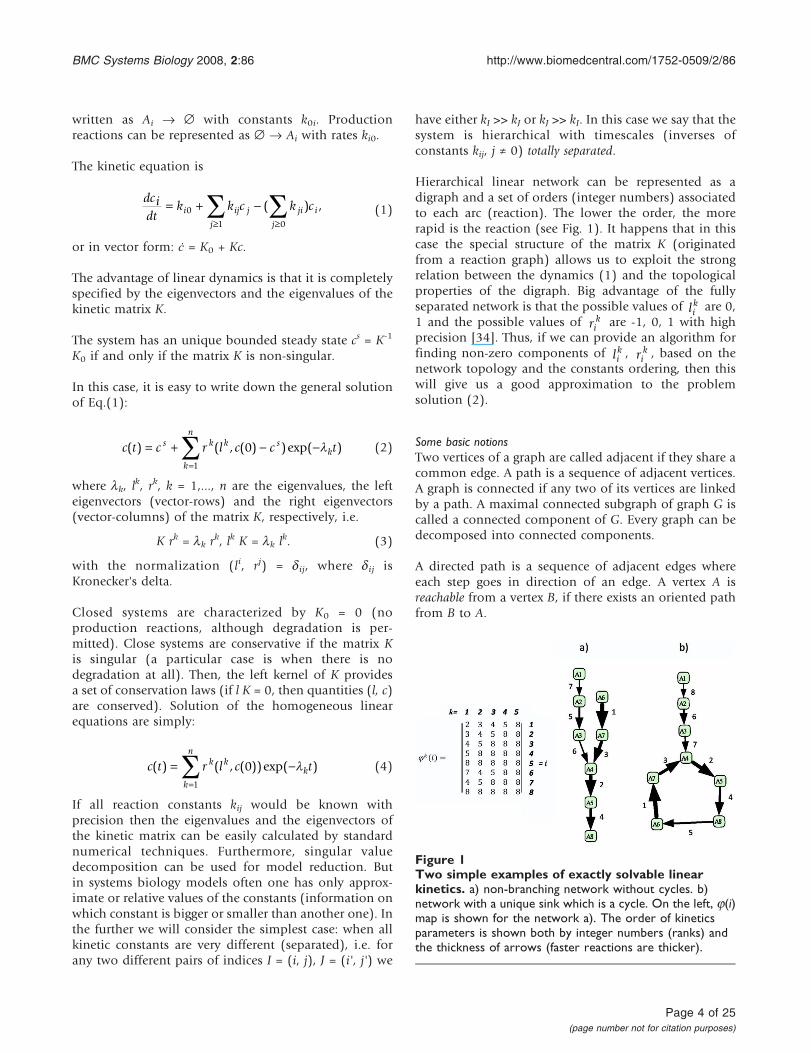
Hierarchical linear network can be represented as adigraph and a set of orders (integer numbers) associatedto each arc (reaction). The lower the order, the morerapid is the reaction (see Fig. 1). It happens that in thiscase the special structure of the matrix K (originatedfrom a reaction graph) allows us to exploit the strongrelation between the dynamics (1) and the topologicalproperties of the digraph. Big advantage of the fullyseparated network is that the possible values of li

k are 0,1 and the possible values of ri

k are -1, 0, 1 with highprecision [34]. Thus, if we can provide an algorithm forfinding non-zero components of li

k , rik , based on the

network topology and the constants ordering, then thiswill give us a good approximation to the problemsolution (2).

Some basic notionsTwo vertices of a graph are called adjacent if they share acommon edge. A path is a sequence of adjacent vertices.A graph is connected if any two of its vertices are linkedby a path. A maximal connected subgraph of graph G iscalled a connected component of G. Every graph can bedecomposed into connected components.

A directed path is a sequence of adjacent edges whereeach step goes in direction of an edge. A vertex A isreachable from a vertex B, if there exists an oriented pathfrom B to A.

Figure 1Two simple examples of exactly solvable linearkinetics. a) non-branching network without cycles. b)network with a unique sink which is a cycle. On the left, j(i)map is shown for the network a). The order of kineticsparameters is shown both by integer numbers (ranks) andthe thickness of arrows (faster reactions are thicker).

BMC Systems Biology 2008, 2:86 http://www.biomedcentral.com/1752-0509/2/86

Page 4 of 25(page number not for citation purposes)

A nonempty set V of graph vertexes forms a sink, if thereare no oriented edges from Ai Œ V to any Aj œ V. Forexample, in the reaction graph A1 ¨ A2 Æ A3 the one-vertex sets {A1} and {A3} are sinks. A sink is minimal ifit does not contain a strictly smaller sink. In the previousexample, {A1}, {A3} are minimal sinks. Minimal sinksare also called ergodic components.

A digraph is strongly connected, if every vertex A isreachable from any other vertex B. Ergodic componentsare maximal strongly connected subgraphs of the graph,but the reverse is not true: there may exist maximalstrongly connected subgraphs that have outgoing edgesand, therefore, are not sinks. If the digraph has nobranching (each vertex has only one successor), then wecan define a deterministic flow (discrete dynamicalsystem) on the set of its vertices. Every vertex is theorigin of an unique directed path.

Basic procedure for approximating eigenvectorsThe algorithm we provide is based on the solution oftwo simplest cases: 1) network without cycles andwithout branching (i.e, there are no vertices with morethan one outgoing edges) (for example, Fig. 1a) and 2)network without branching with a unique sink which is acycle (for example, Fig. 1b).

For the networks without branching, we can simplify thenotation for the kinetic constants, by introducing �i = kij.Also it is useful to introduce a map j (see Fig. 1):

f( ),

,i

j A A

ii j=→⎧

⎨⎩

if there exists

else(5)

Acyclic non-branching networkIn this case, for any vertex Ai there exists an eigenvector.If Ai is a sink vertex (i.e. j(i) = i) then this eigenvalue iszero. If Ai is not a sink (i.e. j(i) ≠ i and reaction Ai Æ Aj

(i) has nonzero rate constant �i) then this eigenvectorcorresponds to eigenvalue -�i. For left and righteigenvectors of K that correspond to Ai we use notationsli (vector-row) and ri (vector-column), correspondingly.

Let us suppose that Af is a sink vertex of the network. Itsassociated right and left eigenvectors corresponding tothe zero eigenvalue are given by:

r

lf j q

jf

jf

jf

q

=

= = >⎧⎨⎪

⎩⎪

d

f1 0

0

, ( )

,

if for some

else

(6)

Generally, right eigenvectors can be constructed byrecurrence starting from the vertex Ai and moving in

the direction of the flow. The construction is in oppositedirection for left eigenvectors.

For right eigenvector ri only coordinates r k ii

f ( ) (k = 0, 1, ..)can have nonzero values, and

rk i

k i ir

j ij i i

k kii

ii

j

k

f f

kfkf k

kfkf k

+ = + −= + −

=

=∏1 1 1

0( ) ( )

( )

( )

( )

( )

kkkf k

kfkf k

ik i i

j ij i ij

k

+ − −=∏1

1( )

( )

( ).

(7)

For left eigenvector li coordinate l ji can have nonzero

value only if there exists such q ≥ 0 that jq (j) = i (this q isunique because the system of reactions has no cycles),and

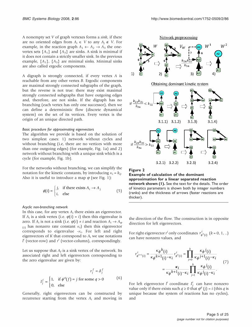
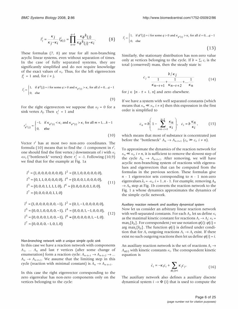
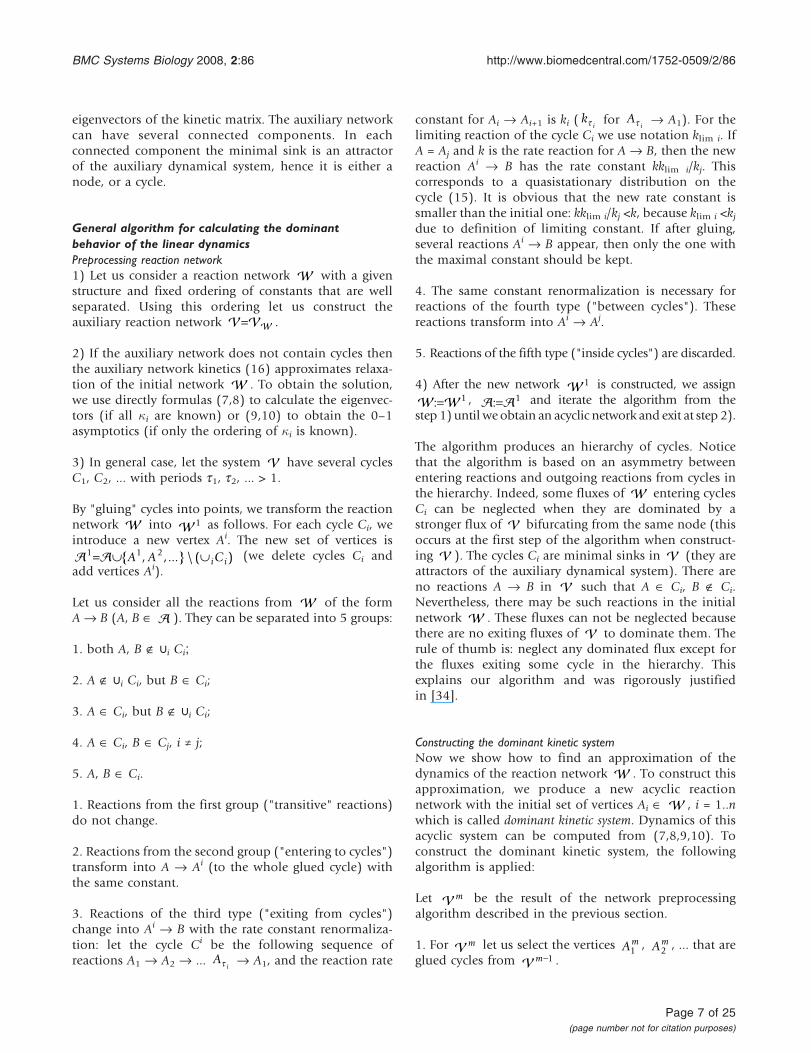
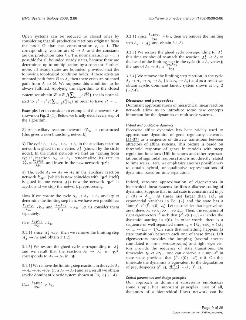
Figure 2Example of calculation of the dominantapproximation for a linear separated reactionnetwork shown (1). See the text for the details. The orderof kinetics parameters is shown both by integer numbers(ranks) and the thickness of arrows (faster reactions arethicker).

BMC Systems Biology 2008, 2:86 http://www.biomedcentral.com/1752-0509/2/86

Page 5 of 25(page number not for citation purposes)

lj

j il

k jk j i

ji

ji

k

q

=−

=−

=

−

∏k

k k

kfkf kf( )

( )

( ).

0

1

(8)

These formulas (7, 8) are true for all non-branchingacyclic linear systems, even without separation of times.In the case of fully separated systems, they aresignificantly simplified and do not require knowledgeof the exact values of �i. Thus, for the left eigenvectorslii = 1 and, for i ≠ j,

lj i q d

ji

qi id

== > > =1 0 0, ( ) ,..

( )if for some and for all f k kf ..

,

q −⎧⎨⎪

⎩⎪

1

0 else

(9)

For the right eigenvectors we suppose that �f = 0 for asink vertex Af. Then ri

i = 1 and

rm k

k

k m

ji i i i i

ff fk k k k

( )( ) ( )

, , ...

,=

− < > = −1 1 1

0

if and for all

eelse

⎧⎨⎪

⎩⎪

(10)

Vector ri has at most two non-zero coordinates. Theformula (10) means that to find the -1 component in ri,one should find the first vertex j downstream of i with �j<�i ("bottleneck" vertex): there r j

i = -1. Following (10,9)we find that for the example at Fig. 1a

l l

l

1 2

3

1 0 0 0 0 0 0 0 0 1 0 0 0 0 0 0

0 1 1 0 0 0

≈ ≈

≈

( , , , , , , , ), ( , , , , , , , ),

( , , , , ,

,, , ), ( , , , , , , , ),

( , , , , , , , ), ( ,

0 0 0 0 0 1 0 0 0 0

0 0 0 1 1 1 1 0 0 0

4

5 6

l

l l

≈

≈ ≈ ,, , , , , , ).

( , , , , , , , )

0 0 0 1 0 0

0 0 0 0 0 1 1 07l ≈

(11)

l l

l

1 2

3

1 0 0 0 0 0 0 1 0 1 1 0 0 0 0 0

0 0 1 0 0

≈ − ≈ −

≈

( , , , , , , , ), ( , , , , , , , ),

( , , , ,

,, , , ), ( , , , , , , , ),

( , , , , , , , ),

0 0 1 0 0 0 1 1 0 0 0

0 0 0 0 1 0 0 1

4

5 6

− ≈ −

≈ −

l

l l ≈≈ −

≈ −

( , , , , , , , ).

( , , , , , , , )

0 0 0 0 0 1 1 0

0 0 0 0 1 0 1 07l

(12)

Non-branching network with a unique simple cyclic sinkIn this case we have a reaction network with componentsA1, ... An and last t vertices (after some change ofenumeration) form a reaction cycle: An-t+1 Æ An-t+2 Æ ...An Æ An-t+1. We assume that the limiting step in thiscycle (reaction with minimal constant) is An Æ An-t+1.

In this case the right eigenvector corresponding to thezero eigenvalue has non-zero components only on thevertices belonging to the cycle:

lj i q d

ji

qi id

== > > =1 0 0, ( ) ,..

( )if for some and for all f k kf ..

,

q −⎧⎨⎪

⎩⎪

1

0 else

(13)

Similarly, the stationary distribution has non-zero valueonly at vertices belonging to the cycle. If b = ∑i ci is thetotal (conserved) mass, then the steady state is:

cb j

n n n

j =

− ++

− ++

/k

k t k t k1

1

1

2

1… (14)

for j Π[n - t + 1, n] and zero elsewhere.

If we have a system with well separated constants (whichmeans that �n ≪ �i, i ≠ n) then this expression in the firstorder is simplified to

c b ni

c b ni

n

i n

n

i= −⎛

⎝⎜⎜

⎞

⎠⎟⎟

== − +

−

∑11

1kk

kk

t

, , (15)

which means that most of substance is concentrated justbefore the "bottleneck" An Æ An-t+1 (cn ≫ ci, i ≠ n).

To approximate the dynamics of the reaction network for�n ≪ �i, i ≠ n, it is sufficient to remove the slowest step ofthe cycle An Æ An-t+1. After removing, we will haveacyclic non-branching system of reactions with eigenva-lues and eigenvectors that can be computed from theformulas in the previous section. These formulas given - 1 eigenvector sets corresponding to n - 1 non-zeroeigenvalues li = -�i, i = 1..n - 1. For example, removing A8

Æ A6 step at Fig. 1b converts the reaction network to theFig. 1 a whose dynamics approximates the dynamics ofthe simple cyclic network.

Auxiliary reaction network and auxiliary dynamical systemNow let us consider an arbitrary linear reaction networkwith well-separated constants. For each Ai, let us define �ias the maximal kinetic constant for reactions Ai Æ Aj: �i =maxj{kji}. For correspondent jwe use notation j(i): j(i) =arg maxj{kji}. The function j(i) is defined under condi-tion that for Ai outgoing reactions Ai Æ Aj exist. If thereexist no such outgoing reactions then let us define j(i) = i.

An auxiliary reaction network is the set of reactions Ai ÆAj(i) with kinetic constants �i. The correspondent kineticequation is

c c ci i i j j

j i

= − +=∑k k

f( )

, (16)

The auxiliary network also defines a auxiliary discretedynamical system i Æ F (i) that is used to compute the

BMC Systems Biology 2008, 2:86 http://www.biomedcentral.com/1752-0509/2/86

Page 6 of 25(page number not for citation purposes)

eigenvectors of the kinetic matrix. The auxiliary networkcan have several connected components. In eachconnected component the minimal sink is an attractorof the auxiliary dynamical system, hence it is either anode, or a cycle.

General algorithm for calculating the dominantbehavior of the linear dynamicsPreprocessing reaction network1) Let us consider a reaction network with a givenstructure and fixed ordering of constants that are wellseparated. Using this ordering let us construct theauxiliary reaction network = .

2) If the auxiliary network does not contain cycles thenthe auxiliary network kinetics (16) approximates relaxa-tion of the initial network . To obtain the solution,we use directly formulas (7,8) to calculate the eigenvec-tors (if all �i are known) or (9,10) to obtain the 0–1asymptotics (if only the ordering of �i is known).

3) In general case, let the system have several cyclesC1, C2, ... with periods t1, t2, ... > 1.

By "gluing" cycles into points, we transform the reactionnetwork into 1 as follows. For each cycle Ci, weintroduce a new vertex Ai. The new set of vertices is 1 1 2= ∪ ∪{ , ,...} \ ( )A A Ci i (we delete cycles Ci andadd vertices Ai).

Let us consider all the reactions from of the formA Æ B (A, B Œ ). They can be separated into 5 groups:

1. both A, B œ ∪i Ci;

2. A œ ∪i Ci, but B Œ Ci;

3. A Œ Ci, but B œ ∪i Ci;

4. A Œ Ci, B Œ Cj, i ≠ j;

5. A, B ΠCi.

1. Reactions from the first group ("transitive" reactions)do not change.

2. Reactions from the second group ("entering to cycles")transform into A Æ Ai (to the whole glued cycle) withthe same constant.

3. Reactions of the third type ("exiting from cycles")change into Ai Æ B with the rate constant renormaliza-tion: let the cycle Ci be the following sequence ofreactions A1 Æ A2 Æ ... A

it Æ A1, and the reaction rate

constant for Ai Æ Ai+1 is ki ( kit for A

it Æ A1). For thelimiting reaction of the cycle Ci we use notation klim i. IfA = Aj and k is the rate reaction for A Æ B, then the newreaction Ai Æ B has the rate constant kklim i/kj. Thiscorresponds to a quasistationary distribution on thecycle (15). It is obvious that the new rate constant issmaller than the initial one: kklim i/kj <k, because klim i <kjdue to definition of limiting constant. If after gluing,several reactions Ai Æ B appear, then only the one withthe maximal constant should be kept.

4. The same constant renormalization is necessary forreactions of the fourth type ("between cycles"). Thesereactions transform into Ai Æ Aj.

5. Reactions of the fifth type ("inside cycles") are discarded.

4) After the new network 1 is constructed, we assign := 1 , := 1 and iterate the algorithm from thestep 1) until we obtain an acyclic network and exit at step 2).

The algorithm produces an hierarchy of cycles. Noticethat the algorithm is based on an asymmetry betweenentering reactions and outgoing reactions from cycles inthe hierarchy. Indeed, some fluxes of entering cyclesCi can be neglected when they are dominated by astronger flux of bifurcating from the same node (thisoccurs at the first step of the algorithm when construct-ing ). The cycles Ci are minimal sinks in (they areattractors of the auxiliary dynamical system). There areno reactions A Æ B in such that A Œ Ci, B œ Ci.Nevertheless, there may be such reactions in the initialnetwork . These fluxes can not be neglected becausethere are no exiting fluxes of to dominate them. Therule of thumb is: neglect any dominated flux except forthe fluxes exiting some cycle in the hierarchy. Thisexplains our algorithm and was rigorously justifiedin [34].

Constructing the dominant kinetic systemNow we show how to find an approximation of thedynamics of the reaction network . To construct thisapproximation, we produce a new acyclic reactionnetwork with the initial set of vertices Ai Π, i = 1..nwhich is called dominant kinetic system. Dynamics of thisacyclic system can be computed from (7,8,9,10). Toconstruct the dominant kinetic system, the followingalgorithm is applied:

Let m be the result of the network preprocessingalgorithm described in the previous section.

1. For m let us select the vertices Am1 , Am

2 , ... that areglued cycles from m−1 .

BMC Systems Biology 2008, 2:86 http://www.biomedcentral.com/1752-0509/2/86

Page 7 of 25(page number not for citation purposes)

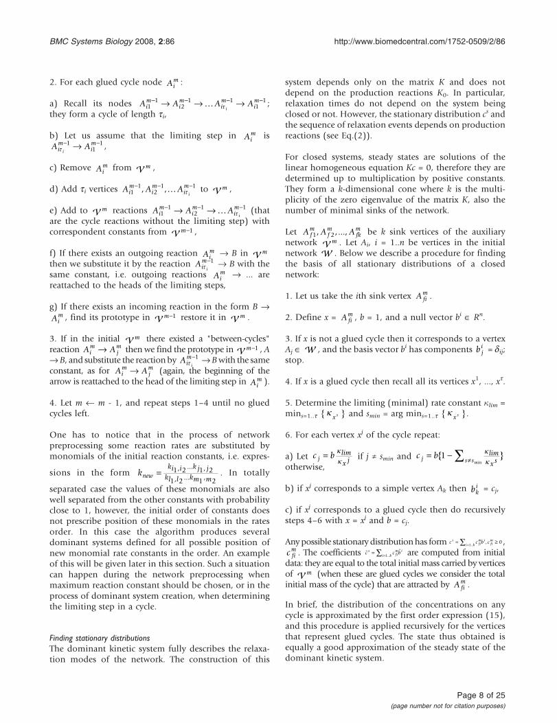
2. For each glued cycle node Aim :

a) Recall its nodes A A A Aim

im

im

im

i11

21 1

11− − − −→ → →… t ;

they form a cycle of length ti,

b) Let us assume that the limiting step in Aim is

A Aim

im

it− −→1

11 ,

c) Remove Aim from m ,

d) Add ti vertices A A Aim

im

im

i11

21 1− − −, ,… t to m ,

e) Add to m reactions A A Aim

im

im

i11

21 1− − −→ →… t (that

are the cycle reactions without the limiting step) withcorrespondent constants from m−1 ,

f) If there exists an outgoing reaction Aim Æ B in m

then we substitute it by the reaction Aim

it−1 Æ B with the

same constant, i.e. outgoing reactions Aim Æ ... are

reattached to the heads of the limiting steps,

g) If there exists an incoming reaction in the form B ÆAi

m , find its prototype in m−1 restore it in m .

3. If in the initial m there existed a "between-cycles"reaction A Ai

mjm→ then we find the prototype in m−1 , A

Æ B, and substitute the reaction by Aim

it−1 ÆBwith the same

constant, as for A Aim

jm→ (again, the beginning of the

arrow is reattached to the head of the limiting step in Aim ).

4. Let m ¨ m - 1, and repeat steps 1–4 until no gluedcycles left.

One has to notice that in the process of networkpreprocessing some reaction rates are substituted bymonomials of the initial reaction constants, i.e. expres-

sions in the form knewki i k j j

kl l km m= 1 2 1 2

1 2 1 2

, ... ,

, ... , . In totally

separated case the values of these monomials are alsowell separated from the other constants with probabilityclose to 1, however, the initial order of constants doesnot prescribe position of these monomials in the ratesorder. In this case the algorithm produces severaldominant systems defined for all possible position ofnew monomial rate constants in the order. An exampleof this will be given later in this section. Such a situationcan happen during the network preprocessing whenmaximum reaction constant should be chosen, or in theprocess of dominant system creation, when determiningthe limiting step in a cycle.

Finding stationary distributionsThe dominant kinetic system fully describes the relaxa-tion modes of the network. The construction of this

system depends only on the matrix K and does notdepend on the production reactions K0. In particular,relaxation times do not depend on the system beingclosed or not. However, the stationary distribution cs andthe sequence of relaxation events depends on productionreactions (see Eq.(2)).

For closed systems, steady states are solutions of thelinear homogeneous equation Kc = 0, therefore they aredetermined up to multiplication by positive constants.They form a k-dimensional cone where k is the multi-plicity of the zero eigenvalue of the matrix K, also thenumber of minimal sinks of the network.

Let A A Afm

fm

fkm

1 2, ,..., be k sink vertices of the auxiliarynetwork m . Let Ai, i = 1..n be vertices in the initialnetwork . Below we describe a procedure for findingthe basis of all stationary distributions of a closednetwork:

1. Let us take the ith sink vertex A fim .

2. Define x = A fim , b = 1, and a null vector bi ΠRn.

3. If x is not a glued cycle then it corresponds to a vertexAj Π, and the basis vector bi has components b j

i = dij;stop.

4. If x is a glued cycle then recall all its vertices x1, ..., xt.

5. Determine the limiting (minimal) rate constant �lim =mins=1..t {k

x s } and smin = arg mins=1..t {kx s }.

6. For each vertex xj of the cycle repeat:

a) Let c bjlim

x j= kk

if j ≠ smin and c bj s slim

x smin= − ≠∑{ }1 k

kotherwise,

b) if xj corresponds to a simple vertex Ak then bki = cj,

c) if xj corresponds to a glued cycle then do recursivelysteps 4–6 with x = xj and b = cj.

Any possible stationary distributionhas form c c b csfim i

i k fim= ≥=∑ 1

0..

, ,c fi

m . The coefficients c c bsfim i

i k= =∑ 1.. are computed from initial

data: they are equal to the total initial mass carried by verticesof m (when these are glued cycles we consider the totalinitial mass of the cycle) that are attracted by A fi

m .

In brief, the distribution of the concentrations on anycycle is approximated by the first order expression (15),and this procedure is applied recursively for the verticesthat represent glued cycles. The state thus obtained isequally a good approximation of the steady state of thedominant kinetic system.

BMC Systems Biology 2008, 2:86 http://www.biomedcentral.com/1752-0509/2/86

Page 8 of 25(page number not for citation purposes)

Open systems can be reduced to closed ones byconsidering that all production reactions originate fromthe node Δ that has concentration c0 = 1. Thecorresponding reaction are Δ Æ Ai and the constantsare the production rates ki0. The normalization c0 = 1 ispossible for all bounded steady states, because these aredetermined up to multiplication by a constant. Further-more, all steady states are bounded, provided that thefollowing topological condition holds: if there exists anoriented path from Δ to Ai, then there exists an orientedpath from Ai to Δ. We suppose this condition to bealways fulfilled. Applying the algorithm to the closed

system we obtain c c c bs sfim i

i k= =∑/( )

.. 01that is normal-

ized to c c c bs sfim i

i k= =∑/( )

.. 01in order to have c s

0 = 1.

Example. Let us consider an example of the network shown on Fig. 2 (1). Below we briefly detail every step ofthe algorithm.

2) An auxiliary reaction network is constructed(this gives a non-branching network);

3) The cycle A3 Æ A4 Æ A5 Æ A3 in the auxiliary reactionnetwork is glued in one vertex A3

1 (shown by the circlenode); In the initial network we find an "exiting fromcycle" reaction A4 Æ A2, renormalize its rate tok k k

k321 24 35

54= and insert in the new network 1 ;

4) The cycle A3 Æ A2 Æ A3 in the auxiliary reactionnetwork V1 (which is now coincides with 1 itself)is glued in one vertex A2

2 ; now the network 2 isacyclic and we stop the network preprocessing.

Now if we restore the cycle A3 Æ A2 Æ A3 and try todetermine the limiting step in it, we have two possibilies:k k

k24 35

54<k32 and k k

k24 35

54> k32. Let us consider them

separately:

Case k kk

24 3554

<k32

3.1.1) Since A31 <k32, then we remove the limiting step

A31 Æ A2 and obtain 3.1.2).

3.1.3) We restore the glued cycle corresponding to A31

and we recall that the reaction A2 Æ A31 in 1

corresponds to A2 Æ A3 in .

3.1.4)We remove the limiting step reaction in the cycle A3

Æ A4 Æ A5 Æ A3 (it is A5 Æ A3) and as a result we obtainacyclic dominant kinetic system shown at Fig. 2 (3.1.4).

Case k kk

24 3554

> k32

3.2.1) Since k kk

24 3554

> k32, then we remove the limiting

step A2 Æ A31 and obtain 3.1.2).

3.2.3) We restore the glued cycle corresponding to A31

this time we should re-attach the reaction A31 Æ A2 to

the head of the limiting step in the cycle (it is A5 vertex);the rate of A5 Æ A2 is k k

k24 35

54.

3.2.4) We remove the limiting step reaction in the cycleA3 Æ A4 Æ A5 Æ A3 (it is A5 Æ A3) and as a result weobtain acyclic dominant kinetic system shown at Fig. 2(3.2.4).

Discussion and perspectivesDominant approximations of hierarchical linear reactionnetwork allow us to introduce some new conceptsimportant for the dynamics of multiscale systems.

Hybrid and qualitative dynamicsPiecewise affine dynamics has been widely used toapproximate dynamics of gene regulatory networks[35-37] as a sequence of discrete transitions betweenattractors of affine systems. This picture is based onthreshold response of genes in models with steepregulation functions (Hill functions and other represen-tations of sigmoidal response) and is not directly relatedto time scales. Here, we emphasize another possible wayto obtain hybrid, or qualitative representations ofdynamics, based on time separation.

Indeed, zero-one approximation of eigenvectors inhierarchical linear systems justifies a discrete coding ofdynamics. Suppose that initial state is concentrated in j0,ci (0) ~ d i j, 0

. At times just larger than 1/lk anexponential vanishes in Eq. (2) and the state has a"jump" -rk (lk, c(0) -cs). Let us consider that eigenvaluesare ordered l1 >> l2 >> ... >> ln-1. Then, the sequence ofright eigenvectors rk such that (lk, c(0) -cs) ≠ 0 codes thedynamics starting in c(0). In other words, there is asequence of well separated times t1 = 1/l1 <<l2 = 1/l2<< ... <<tn-1 = 1/ln-1 such that something happens (astate transition) between each one of these times. Lefteigenvectors provides the lumping (several speciescumulated to form pseudospecies) and right eigenvec-tors provide the sequence of state transitions. Ontimescales tk <t <tk+1 one can observe a jump -rk instate space provided that (lk, c(0) - cs) ≠ 0. On thistimescale the dynamics is equivalent to the degradationof pseudospecies (lk, c), d lk c

dt( , ) = -lk (lk, c).

Critical parameters and design principlesOur approach to dominant subsystems emphasizessome simple but important principles. First of all,dynamics of a hierarchical linear network can be

BMC Systems Biology 2008, 2:86 http://www.biomedcentral.com/1752-0509/2/86

Page 9 of 25(page number not for citation purposes)

specified if a) the topology of the network is given and ifb) to each reaction we associate a positive integerrepresenting order (1 for the most rapid reaction, 2 forthe second most rapid reaction, and so on ...); c) forcyclic topologies, some monomials grouping constantsof several reactions have also to be ordered in the samemanner (which reactions depend both on topology andon initial ordering).

In the process of simplification some reaction pathwaysare dominated and do not appear in the dominantsubsystem. Therefore, the corresponding constants arenot critical for the system: although their orderingmatters for establishing the simplification, their precisevalue have little importance. Because parameters of thedominant subsystem are generally monomials of para-meters of the whole system, critical parameters are thoseparameters that occur in critical monomials. Ourfindings show rather counter-intuitive properties ofcritical and non-critical parameters, that can be usefulas design principles. Thus, in cycles, the limiting step(slowest reaction) has little influence on dynamics(though is important for the steady state). Dynamically,a cycle with separated constants behaves like the chainobtained from the cycle by eliminating the limiting step.In particular, the slowest relaxation time of a cycle is theinverse of its second slowest constant [1, 34].

We should add some words about the relation betweenlinear and non-linear models. Mathematical models ofbiochemical reaction networks in molecular biologycontain with necessity non-linear, non-monomolecularreactions (complex binding, catalysis, etc.). However, thedeveloped algorithms of model reduction for linearnetworks can be useful in systems biology, in severalsituations:

1) When some submechanisms of a complex and non-linearnetwork are linear, given fixed (or slowly changing) valuesof external inputs (boundaries);

2) For approximating non-linear dynamics. For multiscalenonlinear reaction networks the expected dynamicalbehaviour is to be approximated by the system ofdominant networks. These networks may change intime but remain small enough. To give an example, weprovided the Fig. 3S1–3S2 in Additional File 1 demon-strating that in a model of complex reaction network ofNF-�B pathway, containing 17 multimolecular reactions,only two reactions show genuinely non-linear behavior insome windows of time, with two more showing border-line behavior, and all others have well-separated reactantconcentrations in any moment of time. The rigorousjustification of these hybrid approximations for massaction reaction networks will be discussed elsewhere.

Reduction of non-linear multiscale systemsComplex formation is a source of nonlinearity inbiochemical networks. For instance, in signalling, ligandmolecules form complexes with receptors. Transcriptionfactors are often dimers or multimers or are sequesteredby forming complexes with their inhibitors. In theseexamples, the reaction rates are non-linear functions ofthe concentrations of two or more molecules.

To construct a nonlinear reaction network we need thelist of components, = {A1, ..., An} and the list ofreactions (the reaction mechanism):

a bji i jk k

ki

A A→∑∑ , (17)

where j Π[1, r] is the reaction number. Unless reactantsand products belong to compartments of differentvolumes aji, bjk are nonnegative integers (stoichiometriccoefficients). Reactions involving components fromdifferent compartments have non-integer stoichiometry.For instance, a reaction translocating a molecule fromnucleus to the cytosol has stoichiometry (..., 1, kv, ...)where kv is the volume ratio of cytosol to nucleus.

Dynamics of nonlinear networks is described by a systemof differential equations:

dcdt

F c R c SR c R c R cj j

j

r

j j j

j

r

= = = = −=

+ −

=∑ ∑( ) ( ) ( ) ( ( ) ( ))n n

1 1

(18)

vj = bj - aj is the global stoichiometric vector. S is thestoichiometric matrix whose columns are the vectors vj.The reaction rates R j

+ −/ (c) are non-linear functions ofthe concentrations. For instance the mass action lawreads R c k c R c k cj j ii j j ii

ji ji+ + − −= =∏ ∏( ) , ( )a b .

There are no simple rules to relate timescales to reactionconstants of nonlinear models. The units of the inverseconstants of bimolecular reactions are concentrationmultiplied by time and one needs at least one concentra-tion value in order to construct a timescale. Generally,timescales are functions of many reaction constants andconcentration variables. These functions are not necessa-rily smooth. Near bifurcations (for instance, near Hopf orsaddle-node bifurcations), at least one timescale of thesystem diverges for finite changes of the reactionconstants. However, nonlinear biochemical networkshave wide distributions of time-scales, as can be shownby simple (Jacobian based) analysis of models.

Various reduction methods of nonlinear models arebased on projection of the dynamics on a lower

BMC Systems Biology 2008, 2:86 http://www.biomedcentral.com/1752-0509/2/86

Page 10 of 25(page number not for citation purposes)

dimensional invariant manifold [4-8]. The reducedmodels are systems of differential equations, but nolonger networks of chemical reactions. Quasi-equili-brium and quasi-stationarity methods keep the networkstructure of the model and propose lumped reactionmechanisms as dominant subsystems. This approach hassome advantages. Indeed, it leads to more transparentanalysis of the results and of design principles, produceshierarchies of models and facilitates model comparison.Graphical reduction methods using elementary modes,were proposed by Clarke [26] for chemical systems andmore recently in systems biology by Klamt [38]. Similarmethods can be found in [39], from which we haveborrowed the terminology. The choice of the species tobe eliminated and of the reactions to be aggregated, aswell as the calculation of rates of elementary modes haveno theoretical justification in these methods and theirinappropriate use can alter dynamics (for instance, asClarke noticed, the stability of limit cycles is notguaranteed). Thus, in order to have a complete practicalrecipe that applies to multiscale biochemical networkswe need to solve three more problems: detection of rapidspecies, resolution of quasi-stationarity equations andcalculation of reaction rates of the dominantmechanisms.

A major improvement in calculating dominant subsys-tems can be obtained by combining quasi-stationarityand averaging. Averaging techniques are widely used inphysics and chemistry to simplify models by eliminatingfast, oscillating (microscopic) variables [22-24]. Our useof averaging is different, because we employ it to obtainaveraged stationarity equations for slow, non-oscillatingvariables and to eliminate these species. After choosing a"middle" time scale (corresponding to the time resolu-tion of the experiment), we want to reduce all scales thatare faster but also all scales that are slower than thismiddle scale. In order to do that we provide a unifiedframework for species elimination and reaction aggrega-tion, either by quasi-stationarity (fast species) or byaveraged stationarity (slow species).

Let I be the set of indices of intermediate components, thatwill be eliminated. ( )I is the set of reactions that eitherproduce or consume species from I. Rates of ( )I dependon the concentrations of intermediate species and also onthe concentrations of other species, which in the terminol-ogy of Temkin [39] are called terminal. Let T be the set ofindices of terminal species. Terminal species represent thefrontier between the rest of the system and the subsystemsmade of intermediate species. Although instead of terminalthe name boundary species could bemore appropriate, thelatter term has already been employed in systems biologywith a different meaning, which is species whose concen-trations are fixed in a simulation.

Extracting from the matrix S the columns correspondingto the reactions I and the lines corresponding to thespecies and we obtain the intermediate stoichio-metric matrix SI and the terminal stoichiometric matrixST, respectively.

Eliminating fast species: quasi-stationarityIn multiscale biochemical systems, some componentsreact much more rapidly to changes in the environmentthan others. The reasons for the existence of such fastspecies can be multiple. Thus, rapidly transformed orrapidly consumed molecules (for instance those takingpart in metabolic chains or rapid chemical transforma-tions such as phosphorylation), or promoter sitessubmitted to rapid binding/unbinding processes areexamples of fast species. Fast species are good candidatesfor intermediate species. Indeed, it is easy to prove thatthey can be eliminated by quasistationarity. Whenproduction rates are not weak, fast species are thosewhose concentrations are small and well separated fromthe concentrations of other species. Though straightfor-ward, the precise condition connecting quasi-stationarityand smallness of concentrations can not be easily foundin literature, hence we briefly discuss it below.

Let e be a small parameter, representing concentrations.Suppose for simplicity that reactions ( )I are pseudo-monomolecular. This means that SI RI (cI, cT) = KI (cT) cI+ K I

0 (cT), where RI is the restriction of the vector R to theintermediate species. An important assumption isK I

0 (cT) = (1) meaning that the production ofintermediate species is not weak.

Suppose that among the reactions ( )I consumingintermediates, at least some have rates of order (1).This is current, because these reactions produce terminalspecies which have larger concentrations.

Because cI = (e), it means that KI (cT) = (1/e). Thisleads to the following asymptotic:

ε dcIdt

K c c K cI T I I T% % %= +( ) ( )0 (19)

dcIdt

g c cc

I I c= ( , )ε % (20)

where c I = cI/e, K I = eKI = (1), Ic is the complementof I designating species other that I. Intermediate speciesare fast and the system (19) can be reduced usingTikhonov's [40, 41] and Fenichel's [42] results. Accord-ing to these results, after a short laps of time, the systemevolves on an invariant manifold (an invariant manifoldis defined by the property that any trajectory starting inthe manifold stays inside the manifold) which is at

BMC Systems Biology 2008, 2:86 http://www.biomedcentral.com/1752-0509/2/86

Page 11 of 25(page number not for citation purposes)

distance (e) from the quasi-steady state (QSS) mani-fold defined by the quasi-stationarity equations:

K c c K cI T I I T( ) ( )+ =0 0 (21)

Quasi-stationarity equations can be used to expressconcentrations of the intermediate species as functionsof the concentrations of terminal species. If matrix KI hasnot full rank, conservation laws should be added to thequasi-stationarity equations in order to obtain a full ranksystem. Let μ1, ..., μk be a basis of the left kernel of SI (acomplete set of conservation laws). We say that speciesof indices I are quasi-stationary if they approximatelyfulfill the equations:

SI RI (cI, cT) = 0 (22)

and exactly fulfill the conservation laws:

μi iI = Ci, i = 1,..., k, (23)

where Ci are real constants.

Fast, quasi-stationary species are generally difficult todetect. For instance, the strong production conditionK I

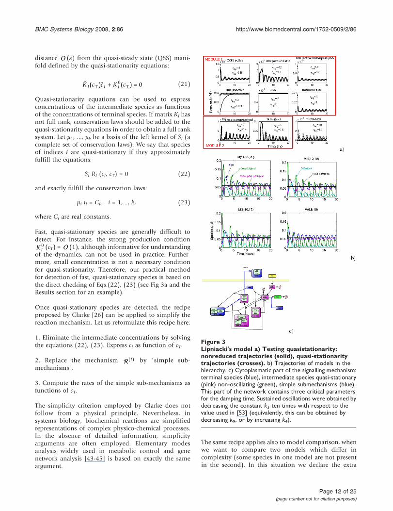
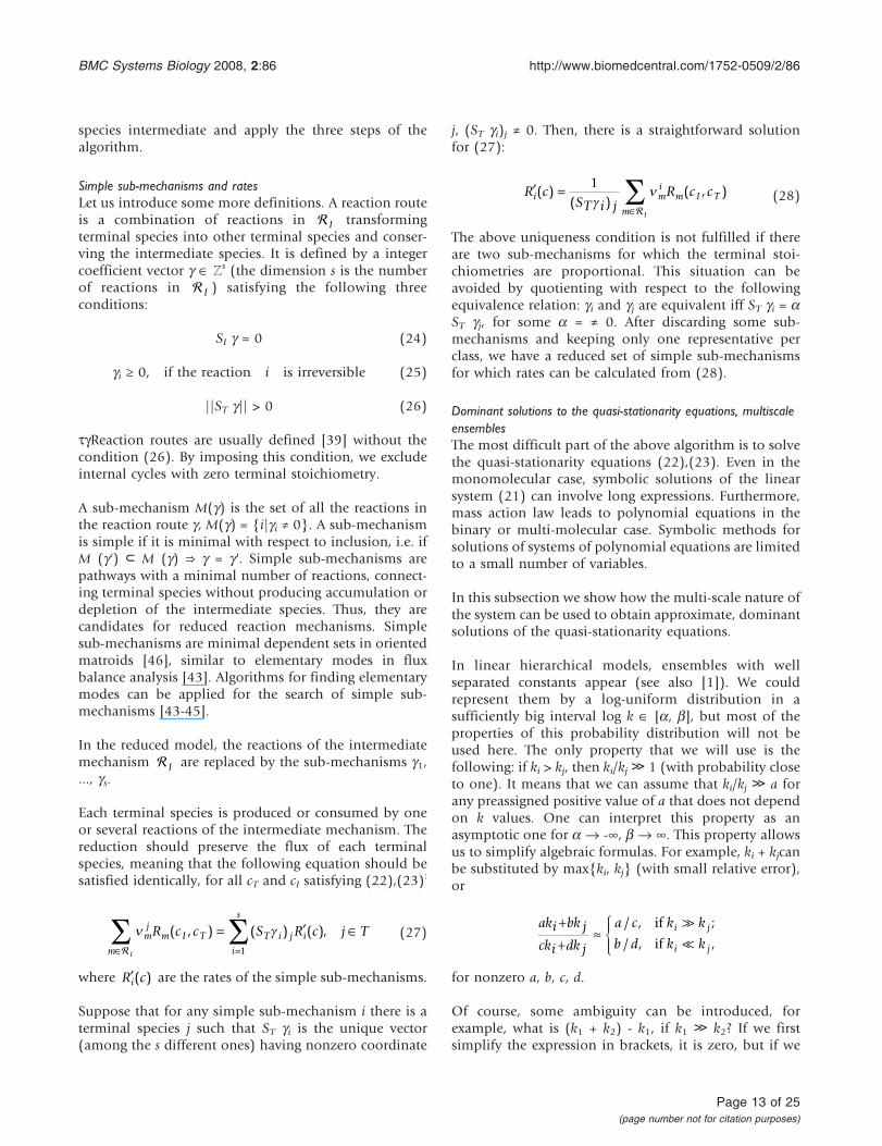
0 (cT) = (1), although informative for understandingof the dynamics, can not be used in practice. Further-more, small concentration is not a necessary conditionfor quasi-stationarity. Therefore, our practical methodfor detection of fast, quasi-stationary species is based onthe direct checking of Eqs.(22), (23) (see Fig 3a and theResults section for an example).

Once quasi-stationary species are detected, the recipeproposed by Clarke [26] can be applied to simplify thereaction mechanism. Let us reformulate this recipe here:

1. Eliminate the intermediate concentrations by solvingthe equations (22), (23). Express cI as function of cT.

2. Replace the mechanism ( )I by "simple sub-mechanisms".

3. Compute the rates of the simple sub-mechanisms asfunctions of cT.

The simplicity criterion employed by Clarke does notfollow from a physical principle. Nevertheless, insystems biology, biochemical reactions are simplifiedrepresentations of complex physico-chemical processes.In the absence of detailed information, simplicityarguments are often employed. Elementary modesanalysis widely used in metabolic control and genenetwork analysis [43-45] is based on exactly the sameargument.

The same recipe applies also to model comparison, whenwe want to compare two models which differ incomplexity (some species in one model are not presentin the second). In this situation we declare the extra

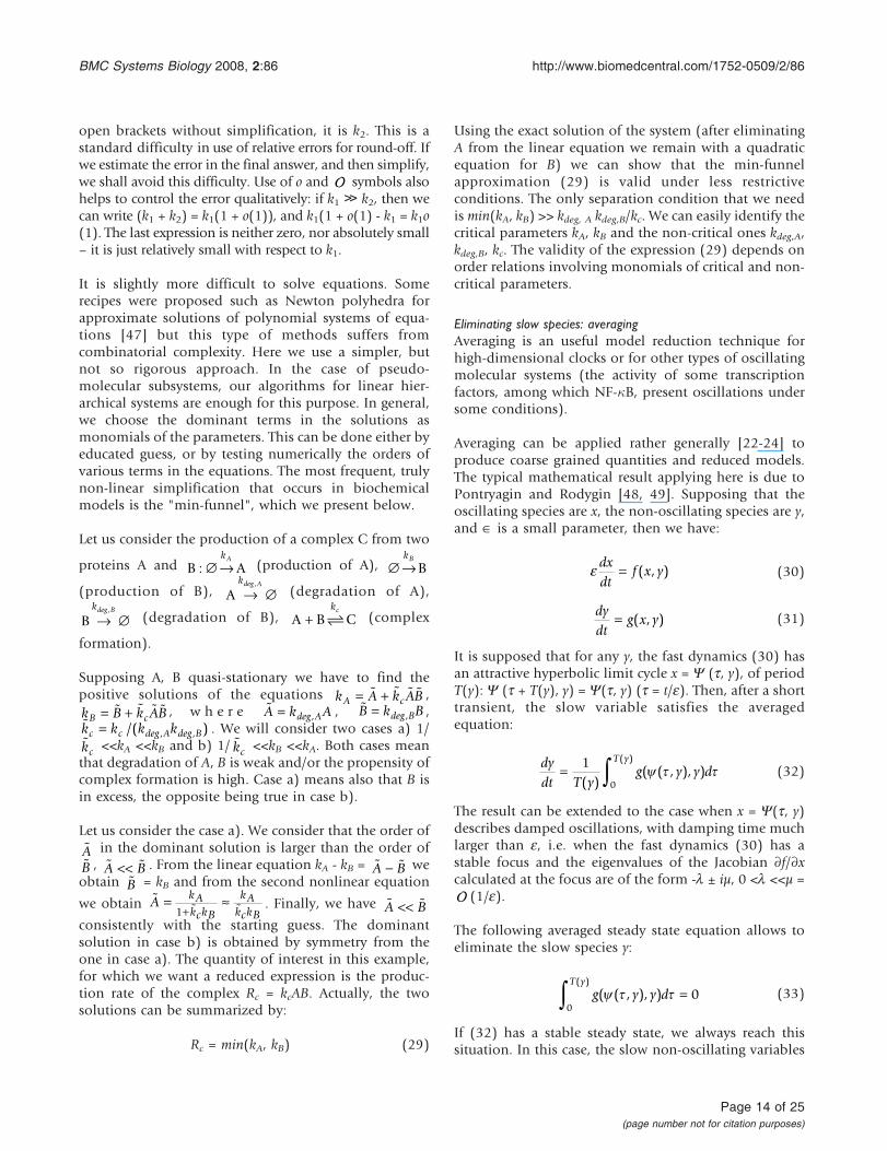
Figure 3Lipniacki's model a) Testing quasistationarity:nonreduced trajectories (solid), quasi-stationaritytrajectories (crosses). b) Trajectories of models in thehierarchy. c) Cytoplasmatic part of the signalling mechanism:terminal species (blue), intermediate species quasi-stationary(pink) non-oscillating (green), simple submechanisms (blue).This part of the network contains three critical parametersfor the damping time. Sustained oscillations were obtained bydecreasing the constant k3 ten times with respect to thevalue used in [53] (equivalently, this can be obtained bydecreasing k9, or by increasing k4).

BMC Systems Biology 2008, 2:86 http://www.biomedcentral.com/1752-0509/2/86

Page 12 of 25(page number not for citation purposes)

species intermediate and apply the three steps of thealgorithm.

Simple sub-mechanisms and ratesLet us introduce some more definitions. A reaction routeis a combination of reactions in I transformingterminal species into other terminal species and conser-ving the intermediate species. It is defined by a integercoefficient vector g Œ ℤs (the dimension s is the numberof reactions in I ) satisfying the following threeconditions:

SI g = 0 (24)

gi ≥ 0, if the reaction i is irreversible (25)

||ST g|| > 0 (26)

tgReaction routes are usually defined [39] without thecondition (26). By imposing this condition, we excludeinternal cycles with zero terminal stoichiometry.

A sub-mechanism M(g) is the set of all the reactions inthe reaction route g, M(g) = {i|gi ≠ 0}. A sub-mechanismis simple if it is minimal with respect to inclusion, i.e. ifM (g') ⊂ M (g) ⇒ g = g'. Simple sub-mechanisms arepathways with a minimal number of reactions, connect-ing terminal species without producing accumulation ordepletion of the intermediate species. Thus, they arecandidates for reduced reaction mechanisms. Simplesub-mechanisms are minimal dependent sets in orientedmatroids [46], similar to elementary modes in fluxbalance analysis [43]. Algorithms for finding elementarymodes can be applied for the search of simple sub-mechanisms [43-45].

In the reduced model, the reactions of the intermediatemechanism I are replaced by the sub-mechanisms g1,..., gs.

Each terminal species is produced or consumed by oneor several reactions of the intermediate mechanism. Thereduction should preserve the flux of each terminalspecies, meaning that the following equation should besatisfied identically, for all cT and cI satisfying (22),(23):

n gmj

m I T

m

T i j i

i

s

R c c S R c j T

I

( , ) ( ) ( ),∈ =∑ ∑= ′ ∈

1

(27)

where ′R ci( ) are the rates of the simple sub-mechanisms.

Suppose that for any simple sub-mechanism i there is aterminal species j such that ST gi is the unique vector(among the s different ones) having nonzero coordinate

j, (ST gi)j ≠ 0. Then, there is a straightforward solutionfor (27):

′ =∈∑R c

ST i jR c ci m

im I T

m I

( )( )

( , )1g

n

(28)

The above uniqueness condition is not fulfilled if thereare two sub-mechanisms for which the terminal stoi-chiometries are proportional. This situation can beavoided by quotienting with respect to the followingequivalence relation: gi and gj are equivalent iff ST gi = aST gj, for some a = ≠ 0. After discarding some sub-mechanisms and keeping only one representative perclass, we have a reduced set of simple sub-mechanismsfor which rates can be calculated from (28).

Dominant solutions to the quasi-stationarity equations, multiscaleensemblesThe most difficult part of the above algorithm is to solvethe quasi-stationarity equations (22),(23). Even in themonomolecular case, symbolic solutions of the linearsystem (21) can involve long expressions. Furthermore,mass action law leads to polynomial equations in thebinary or multi-molecular case. Symbolic methods forsolutions of systems of polynomial equations are limitedto a small number of variables.

In this subsection we show how the multi-scale nature ofthe system can be used to obtain approximate, dominantsolutions of the quasi-stationarity equations.

In linear hierarchical models, ensembles with wellseparated constants appear (see also [1]). We couldrepresent them by a log-uniform distribution in asufficiently big interval log k Œ [a, b], but most of theproperties of this probability distribution will not beused here. The only property that we will use is thefollowing: if ki > kj, then ki/kj ≫ 1 (with probability closeto one). It means that we can assume that ki/kj ≫ a forany preassigned positive value of a that does not dependon k values. One can interpret this property as anasymptotic one for a Æ -∞, b Æ ∞. This property allowsus to simplify algebraic formulas. For example, ki + kjcanbe substituted by max{ki, kj} (with small relative error),or

aki bk jcki dk j

a c k k

b d k ki j

i j

++

≈⎧⎨⎪

⎩⎪

/ , ;

/ , ,

if

if

for nonzero a, b, c, d.

Of course, some ambiguity can be introduced, forexample, what is (k1 + k2) - k1, if k1 ≫ k2? If we firstsimplify the expression in brackets, it is zero, but if we

BMC Systems Biology 2008, 2:86 http://www.biomedcentral.com/1752-0509/2/86

Page 13 of 25(page number not for citation purposes)

open brackets without simplification, it is k2. This is astandard difficulty in use of relative errors for round-off. Ifwe estimate the error in the final answer, and then simplify,we shall avoid this difficulty. Use of o and symbols alsohelps to control the error qualitatively: if k1 ≫ k2, then wecan write (k1 + k2) = k1(1 + o(1)), and k1(1 + o(1) - k1 = k1o(1). The last expression is neither zero, nor absolutely small– it is just relatively small with respect to k1.

It is slightly more difficult to solve equations. Somerecipes were proposed such as Newton polyhedra forapproximate solutions of polynomial systems of equa-tions [47] but this type of methods suffers fromcombinatorial complexity. Here we use a simpler, butnot so rigorous approach. In the case of pseudo-molecular subsystems, our algorithms for linear hier-archical systems are enough for this purpose. In general,we choose the dominant terms in the solutions asmonomials of the parameters. This can be done either byeducated guess, or by testing numerically the orders ofvarious terms in the equations. The most frequent, trulynon-linear simplification that occurs in biochemicalmodels is the "min-funnel", which we present below.

Let us consider the production of a complex C from two

proteins A and B A: ∅→kA

(production of A), ∅→kB

B

(production of B), A → ∅kdeg A,

(degradation of A),

B → ∅kdeg B,

(degradation of B), A B C+kc

(complex

formation).

Supposing A, B quasi-stationary we have to find thepositive solutions of the equations k A k ABA c= + ,k B k ABB c= + , w h e r e A k Adeg A= , , B k Bdeg B= , ,k k k kc c deg A deg B= /( ), , . We will consider two cases a) 1/kc <<kA <<kB and b) 1/ kc <<kB <<kA. Both cases meanthat degradation of A, B is weak and/or the propensity ofcomplex formation is high. Case a) means also that B isin excess, the opposite being true in case b).

Let us consider the case a). We consider that the order of

A in the dominant solution is larger than the order ofB , A B<< . From the linear equation kA - kB = A B− weobtain B = kB and from the second nonlinear equation

we obtain A kAkckB

kAkckB

= ≈+1

. Finally, we have A B<<consistently with the starting guess. The dominantsolution in case b) is obtained by symmetry from theone in case a). The quantity of interest in this example,for which we want a reduced expression is the produc-tion rate of the complex Rc = kcAB. Actually, the twosolutions can be summarized by:

Rc = min(kA, kB) (29)

Using the exact solution of the system (after eliminatingA from the linear equation we remain with a quadraticequation for B) we can show that the min-funnelapproximation (29) is valid under less restrictiveconditions. The only separation condition that we needis min(kA, kB) >> kdeg, A kdeg,B/kc. We can easily identify thecritical parameters kA, kB and the non-critical ones kdeg,A,kdeg,B, kc. The validity of the expression (29) depends onorder relations involving monomials of critical and non-critical parameters.

Eliminating slow species: averagingAveraging is an useful model reduction technique forhigh-dimensional clocks or for other types of oscillatingmolecular systems (the activity of some transcriptionfactors, among which NF-�B, present oscillations undersome conditions).

Averaging can be applied rather generally [22-24] toproduce coarse grained quantities and reduced models.The typical mathematical result applying here is due toPontryagin and Rodygin [48, 49]. Supposing that theoscillating species are x, the non-oscillating species are y,and Πis a small parameter, then we have:

ε dxdt

f x y= ( , ) (30)

dydt

g x y= ( , ) (31)

It is supposed that for any y, the fast dynamics (30) hasan attractive hyperbolic limit cycle x = Y (t, y), of periodT(y): Y (t + T(y), y) = Y(t, y) (t = t/e). Then, after a shorttransient, the slow variable satisfies the averagedequation:

dydt T y

g y y dT y

= ∫1

0( )( ( , ), )

( )y t t (32)

The result can be extended to the case when x = Y(t, y)describes damped oscillations, with damping time muchlarger than e, i.e. when the fast dynamics (30) has astable focus and the eigenvalues of the Jacobian ∂f/∂xcalculated at the focus are of the form -l ± iμ, 0 <l <<μ = (1/e).

The following averaged steady state equation allows toeliminate the slow species y:

g y y dT y

( ( , ), )( )

y t t =∫ 00

(33)

If (32) has a stable steady state, we always reach thissituation. In this case, the slow non-oscillating variables

BMC Systems Biology 2008, 2:86 http://www.biomedcentral.com/1752-0509/2/86

Page 14 of 25(page number not for citation purposes)

y are constant in time and can be considered to beconserved, which has two significant consequences.

First, Eq.(33) restores conservation. Slow variables areoften the result of broken conservation laws. In fact, inbiological open systems, nothing is conserved. Conser-vation laws result from balancing production anddegradation either passively (slow processes) or actively(feed-back). Thus, we can ignore production anddegradation of molecules whose level is rigorouslycontrolled. Eq.(33) describes such a case.

Second, (33) are averaged steady state equations for theslow variables. If slow variables y reach stationarity, theonly variables that change in time are the oscillatingvariables x. Eq.(30) describes the dynamics of x,considering that y satisfies (33). For oscillators, averagingprovides a way to eliminate slow non-oscillating vari-ables, which is formally equivalent to quasi-stationarityand represents a new case of applicability of Clarke'smethod. The difference between the two cases is that weeliminate fast variables by solving quasi-stationarityequations and we eliminate slow variables by solvingaveraged stationarity equations. Thus, intermediate non-oscillating variables are expressed in terms of onlynon-oscillating terminal variables. If there are nonon-oscillating terminal variables, then non-oscillatingintermediates become conserved quantities.

Results and discussionMethodologyIn this section, we demonstrate hierarchical modelreduction, model comparison and critical parameteridentification. Critical parameters are identified duringthe reduction procedure.

Model reduction starts with a complex model, fromwhich we obtain a hierarchy of reduced models byeliminating various intermediate species. The intermedi-ate species are either quasi-stationary species (ingeneral), or non-oscillating species (for oscillators). Thecomplexity of a model is quantified by three integers. Amodel with n species, r reactions and p parameters isdesignated by M(n, r, p). Our conception about systemsbiology models is summarized by the following idea.Instead of providing a single model, it is better toprovide a hierarchy of models, and the relations betweenthem. Depending on the application, we can choose themost appropriate model in the hierarchy or coupleseveral simple models into a larger model.

The number of parameters in a model are obtained asfollows. If the elementary reactions follow mass actionlaw kinetics, there are nk = 2nr + ni kinetic constants,

where nr, ni are the numbers of reversible and irreversiblereactions. Reactions with kinetic constants zero are notconsidered in the counting. Each one of the nc conserva-tion laws adds an extra parameter, the value of theconserved quantity. These values follow from initial dataand are important parameters for the dynamics. Formulti-compartment models, the ratios of the compart-ments volumes (in the example below there is only oneratio kv, the cytoplasm to nucleus volume ratio) are extraparameters. Thus p = n

k+ nc + 1.

Model comparison has a similar flowchart. By modelcomparison we understand a) mapping one model toanother one by model reduction or mapping each modelto a third one, closest in some sense to both; b) comparepredictions of the models (for instance, about how thesystem responds to perturbations) for sets of parametersrelated one to the other by the mapping at a). In thiscase, the choice of intermediate species is dictated by thedifferences between the models to be compared.

Hierarchy of models for NF-�B signallingThe transcription factor NF-�B is involved in a widediversity of domains such as the immune and inflam-matory responses, cell survival and apoptosis, cellularstress and neuro-degenerative diseases, cancer anddevelopment. NF-�B is sequestered in the cytoplasm byinactivating proteins named I�B. Upon signalling, I�Bmolecules are phosphorylated by a kinase complex, thenubiquitinylated, and finally degraded by the proteaso-mal complex. NF-�B bound to I�B molecules is thentransported to the nucleus to activate its target genes.There are known five members of the NF-�B family inmammals, Rel (c-rel), RelA (p65), RelB, NF-�B1 (p50and its precursor p105) and NF-�B2 (p52 and itsprecursor p100). This generates a large combinatorialcomplexity of dimers, affinities and transcriptionalcapabilities. I�B family comprises seven members inmammals (I�Ba, I�Bb, I�Be, I�Bg, Bcl-3) [50]. All theseinhibitors display different affinities for NF-�B dimers,multiplying the combinatorial complexity. Moreover,the gene coding for I�Ba, is transcriptionally activated byNF-�B. This negative feed-back loop can give rise tooscillations of the activity of NF-�B [51, 52]. Phosphor-ylation of I�Ba upon signalling is provided by a kinasescomplex that includes IKKa and IKKb (I�B Kinase, alsonamed IKK1 and IKK2), associated to a regulatingprotein NEMO (NF-�B Essential Modulator, also calledIKKg). Therefore, it is clear that understanding such acomplex biological system requires modeling. Severalmathematical models of NF-�B have been published.The first model described a single NF-�B molecule,which binds to I�Ba, I�Bb and I�Be. This workdemonstrated oscillations in NF-�B activity, confirmed

BMC Systems Biology 2008, 2:86 http://www.biomedcentral.com/1752-0509/2/86

Page 15 of 25(page number not for citation purposes)

by experimental data [51]. The model set by [53]included in addition an A20 molecule whose productionis enhanced upon NF-�B stimulation, and whichnegatively regulates IKK activity. A third model analyzedthe critical parameters necessary for maintaining oscilla-tions, with given amplitude and frequency [54]. Inaddition, a minimal simplified model was also set tostudy the oscillations of the NF-�B module [55]. Wepropose here a fourth, new model, with more complexdescriptions that takes into account transcription,translation and degradation of different NF-�B units.

In our model, NF-�B is considered to be made of twosubunits, p50 and p65. All combinations of these subunitsare allowed, including two homodimers p50:p50, p65:p65and one heterodimer p50:p65. The three dimers of NF-�Bare characterized by different affinities for DNA sites, andassociate differentially to I�Ba, b and e, generating thus 9species with different abundances and characteristics uponsignalling and degradation. The production of the dimerp65 is considered under control of a transcription factorFTAy, which represents a simplification of many transcrip-tion factors supposed to activate this promoter. p50 isproduced from a precursor molecule p105. The transcrip-tion factor FTAx binds to the promoter of p105 to activate itstranscription at a basal level. Similarly to FTAy, this factorrepresents the sum of individual activities due to severaltranscription factors contributing to the basal activity of thispromoter. As the p105 gene is activated byNF-�B, this factorcan also bind to the p105 promoter and activate thetranscription above the basal level. Promoter of I�B iscontrolled by NF-�B and FTAz in a similar way as it is p105.In addition, it was supposed that nuclear I�B can come andbind to NF-�B when this is on the promoter of I�B or ofp105. Once the complex formed this can unbind from theDNA, takingNF-�B away. The kinase activation/inactivationmodule including interactionswithA20was borrowed from[53]. Let us notice that transcription regulation modules arevery simplified and do not take into account specificities ofeukaryotic regulation (existence of several binding sites,enhancers, etc).

Initiation [56, 57] and elongation [58-60] for transcrip-tion and translation rates come from previous studieswhich were more recently re-examined [61]. Binding andunbinding constants for NF-�B subunits come eitherfrom literature [62-64] or from previous models [51, 53].

We should signal large uncertainty concerning values ofconstants. For example, the rate of degradation of I�Bwas assumed to be independent of the state of themolecule, either free or bound to NF-�B. This led to apoor fit of computational simulations of the NF-�Bsignalling module. The rate was newly measured in vivoand led to better fits of I�B levels and basal NF-�B

activity [65]. This motivated us to determine whichparameters of the model are critical and should beknown with precision and which ones are not critical.

A simplified version of the model (considering only theI�Ba inhibitor) is given in Table 1.

Model reductionAs an illustration of the model reduction flowchart, weobtain from the model proposed by Lipniacki [53] aseries of simpler models. This model is (14, 25, 28)in our hierarchy: it contains only one reversible reactionand the total NF-�B quantity is conserved nc = nr = 1. Thedescription of the reactions can be found in Table 1(Lipniacki's model is a submodel of our model).

The model was forced to function in a stronglyoscillating regime. This situation is the most unfavorablefor the simple version of Clarke's method which isdoomed to shorten delays and to destabilize oscillationswhen intermediates are not appropriately chosen. Thus,it represents a good test for our method. First, we identifyquasi-stationary and non-oscillating species. We definelog-average concentration clog = log <c > and the log-amplitude alog = min(log max(c) - clog, clog - log min(c))(the minimum is to avoid divergence when min(c) = 0).Species whose log-amplitudes are low and well separatedfrom other values are declared non-oscillating. In orderto detect quasi-stationary species, for each species Ai wecompare two trajectories (concentrations as functions oftime): a) the trajectory in the unreduced model b) thetrajectory of Ai calculated from the trajectories of thespecies influencing Ai by using the quasi-stationarityequation (22) for I = {i}. The two trajectories must beclose one to another for quasi-stationary species (exceptfor a short transition region), see Fig. 3a). Hausdorffdistance between the two trajectories can be used to detectquasi-stationary species for automatic computation.Non-oscillating species could also satisfy this criterion,but after a larger transition region, because they are slow(see the behavior of IKK|inactive in Fig. 3a)).

These procedures allow to identify 7 quasi-stationaryspecies (IKK|active, IKK, IKK|active:IkBa, IKK|active:IkBa:p50:p65, IkBa@ncl, IkBa:p50:p65@ncl, p50:p65@csl)and one non-oscillating species (IKK|inactive). Twospecies with small concentration (mRNAA20,mRNAIkBa) are not quasi-stationary, as their relaxationtime can be compared to the period of the oscillations.The smallness of their concentration is not a conse-quence of rapid consumption, but of small production(transcription) rate. Two species with large concentrationare quasi-stationary (IkBa@ncl, p50:p65@csl).

BMC Systems Biology 2008, 2:86 http://www.biomedcentral.com/1752-0509/2/86

Page 16 of 25(page number not for citation purposes)

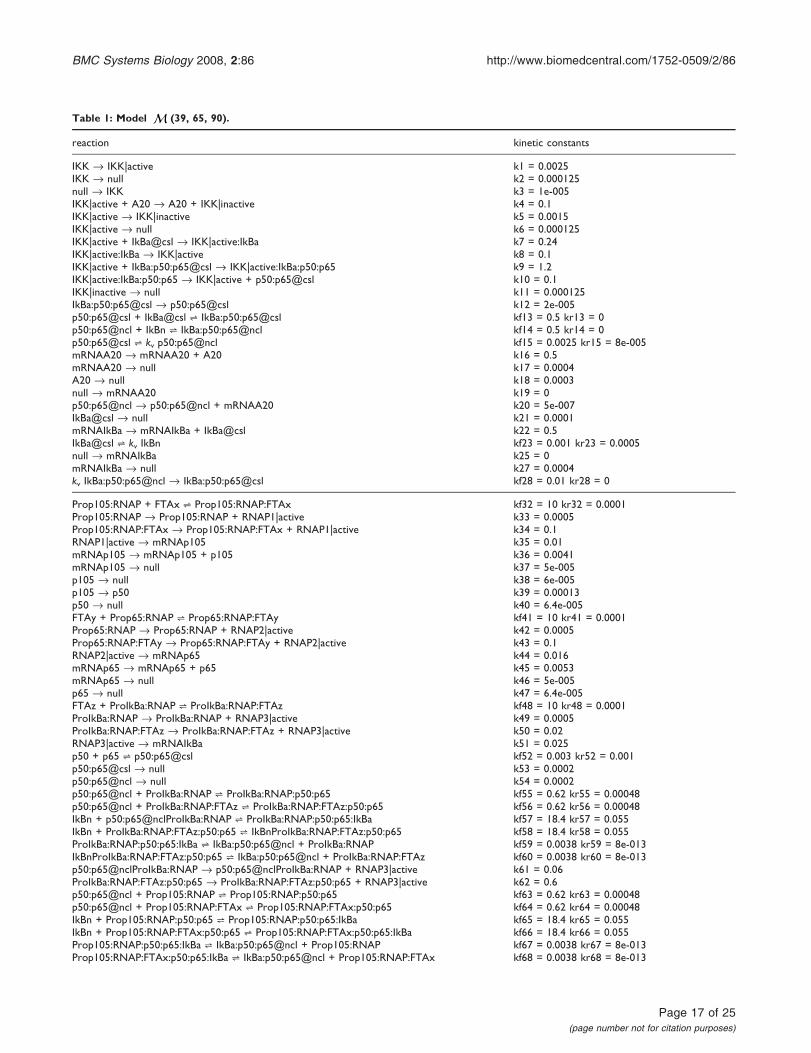
Table 1: Model (39, 65, 90).

reaction kinetic constants

IKK Æ IKK|active k1 = 0.0025IKK Æ null k2 = 0.000125null Æ IKK k3 = 1e-005IKK|active + A20 Æ A20 + IKK|inactive k4 = 0.1IKK|active Æ IKK|inactive k5 = 0.0015IKK|active Æ null k6 = 0.000125IKK|active + IkBa@csl Æ IKK|active:IkBa k7 = 0.24IKK|active:IkBa Æ IKK|active k8 = 0.1IKK|active + IkBa:p50:p65@csl Æ IKK|active:IkBa:p50:p65 k9 = 1.2IKK|active:IkBa:p50:p65 Æ IKK|active + p50:p65@csl k10 = 0.1IKK|inactive Æ null k11 = 0.000125IkBa:p50:p65@csl Æ p50:p65@csl k12 = 2e-005p50:p65@csl + IkBa@csl ⇌ IkBa:p50:p65@csl kf13 = 0.5 kr13 = 0p50:p65@ncl + IkBn ⇌ IkBa:p50:p65@ncl kf14 = 0.5 kr14 = 0p50:p65@csl ⇌ kv p50:p65@ncl kf15 = 0.0025 kr15 = 8e-005mRNAA20 Æ mRNAA20 + A20 k16 = 0.5mRNAA20 Æ null k17 = 0.0004A20 Æ null k18 = 0.0003null Æ mRNAA20 k19 = 0p50:p65@ncl Æ p50:p65@ncl + mRNAA20 k20 = 5e-007IkBa@csl Æ null k21 = 0.0001mRNAIkBa Æ mRNAIkBa + IkBa@csl k22 = 0.5IkBa@csl ⇌ kv IkBn kf23 = 0.001 kr23 = 0.0005null Æ mRNAIkBa k25 = 0mRNAIkBa Æ null k27 = 0.0004kv IkBa:p50:p65@ncl Æ IkBa:p50:p65@csl kf28 = 0.01 kr28 = 0

Prop105:RNAP + FTAx ⇌ Prop105:RNAP:FTAx kf32 = 10 kr32 = 0.0001Prop105:RNAP Æ Prop105:RNAP + RNAP1|active k33 = 0.0005Prop105:RNAP:FTAx Æ Prop105:RNAP:FTAx + RNAP1|active k34 = 0.1RNAP1|active Æ mRNAp105 k35 = 0.01mRNAp105 Æ mRNAp105 + p105 k36 = 0.0041mRNAp105 Æ null k37 = 5e-005p105 Æ null k38 = 6e-005p105 Æ p50 k39 = 0.00013p50 Æ null k40 = 6.4e-005FTAy + Prop65:RNAP ⇌ Prop65:RNAP:FTAy kf41 = 10 kr41 = 0.0001Prop65:RNAP Æ Prop65:RNAP + RNAP2|active k42 = 0.0005Prop65:RNAP:FTAy Æ Prop65:RNAP:FTAy + RNAP2|active k43 = 0.1RNAP2|active Æ mRNAp65 k44 = 0.016mRNAp65 Æ mRNAp65 + p65 k45 = 0.0053mRNAp65 Æ null k46 = 5e-005p65 Æ null k47 = 6.4e-005FTAz + ProIkBa:RNAP ⇌ ProIkBa:RNAP:FTAz kf48 = 10 kr48 = 0.0001ProIkBa:RNAP Æ ProIkBa:RNAP + RNAP3|active k49 = 0.0005ProIkBa:RNAP:FTAz Æ ProIkBa:RNAP:FTAz + RNAP3|active k50 = 0.02RNAP3|active Æ mRNAIkBa k51 = 0.025p50 + p65 ⇌ p50:p65@csl kf52 = 0.003 kr52 = 0.001p50:p65@csl Æ null k53 = 0.0002p50:p65@ncl Æ null k54 = 0.0002p50:p65@ncl + ProIkBa:RNAP ⇌ ProIkBa:RNAP:p50:p65 kf55 = 0.62 kr55 = 0.00048p50:p65@ncl + ProIkBa:RNAP:FTAz ⇌ ProIkBa:RNAP:FTAz:p50:p65 kf56 = 0.62 kr56 = 0.00048IkBn + p50:p65@nclProIkBa:RNAP ⇌ ProIkBa:RNAP:p50:p65:IkBa kf57 = 18.4 kr57 = 0.055IkBn + ProIkBa:RNAP:FTAz:p50:p65 ⇌ IkBnProIkBa:RNAP:FTAz:p50:p65 kf58 = 18.4 kr58 = 0.055ProIkBa:RNAP:p50:p65:IkBa ⇌ IkBa:p50:p65@ncl + ProIkBa:RNAP kf59 = 0.0038 kr59 = 8e-013IkBnProIkBa:RNAP:FTAz:p50:p65 ⇌ IkBa:p50:p65@ncl + ProIkBa:RNAP:FTAz kf60 = 0.0038 kr60 = 8e-013p50:p65@nclProIkBa:RNAP Æ p50:p65@nclProIkBa:RNAP + RNAP3|active k61 = 0.06ProIkBa:RNAP:FTAz:p50:p65 Æ ProIkBa:RNAP:FTAz:p50:p65 + RNAP3|active k62 = 0.6p50:p65@ncl + Prop105:RNAP ⇌ Prop105:RNAP:p50:p65 kf63 = 0.62 kr63 = 0.00048p50:p65@ncl + Prop105:RNAP:FTAx ⇌ Prop105:RNAP:FTAx:p50:p65 kf64 = 0.62 kr64 = 0.00048IkBn + Prop105:RNAP:p50:p65 ⇌ Prop105:RNAP:p50:p65:IkBa kf65 = 18.4 kr65 = 0.055IkBn + Prop105:RNAP:FTAx:p50:p65 ⇌ Prop105:RNAP:FTAx:p50:p65:IkBa kf66 = 18.4 kr66 = 0.055Prop105:RNAP:p50:p65:IkBa ⇌ IkBa:p50:p65@ncl + Prop105:RNAP kf67 = 0.0038 kr67 = 8e-013Prop105:RNAP:FTAx:p50:p65:IkBa ⇌ IkBa:p50:p65@ncl + Prop105:RNAP:FTAx kf68 = 0.0038 kr68 = 8e-013

BMC Systems Biology 2008, 2:86 http://www.biomedcentral.com/1752-0509/2/86

Page 17 of 25(page number not for citation purposes)

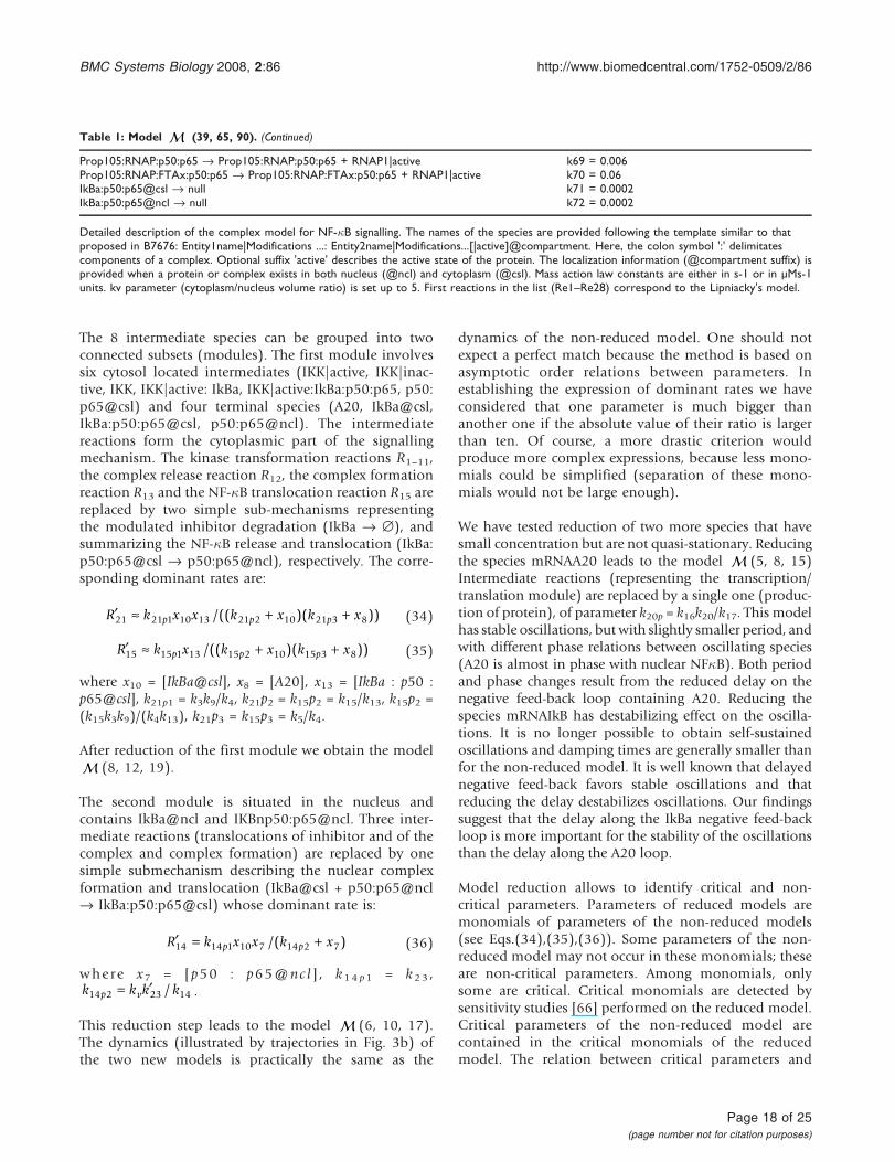
The 8 intermediate species can be grouped into twoconnected subsets (modules). The first module involvessix cytosol located intermediates (IKK|active, IKK|inac-tive, IKK, IKK|active: IkBa, IKK|active:IkBa:p50:p65, p50:p65@csl) and four terminal species (A20, IkBa@csl,IkBa:p50:p65@csl, p50:p65@ncl). The intermediatereactions form the cytoplasmic part of the signallingmechanism. The kinase transformation reactions R1–11,the complex release reaction R12, the complex formationreaction R13 and the NF-�B translocation reaction R15 arereplaced by two simple sub-mechanisms representingthe modulated inhibitor degradation (IkBa Æ Δ), andsummarizing the NF-�B release and translocation (IkBa:p50:p65@csl Æ p50:p65@ncl), respectively. The corre-sponding dominant rates are:

′ ≈ + +R k x x k x k xp p p21 21 1 10 13 21 2 10 21 3 8/(( )( )) (34)

′ ≈ + +R k x k x k xp p p15 15 1 13 15 2 10 15 3 8/(( )( )) (35)

where x10 = [IkBa@csl], x8 = [A20], x13 = [IkBa : p50 :p65@csl], k21p1 = k3k9/k4, k21p2 = k15p2 = k15/k13, k15p2 =(k15k3k9)/(k4k13), k21p3 = k15p3 = k5/k4.

After reduction of the first module we obtain the model (8, 12, 19).

The second module is situated in the nucleus andcontains IkBa@ncl and IKBnp50:p65@ncl. Three inter-mediate reactions (translocations of inhibitor and of thecomplex and complex formation) are replaced by onesimple submechanism describing the nuclear complexformation and translocation (IkBa@csl + p50:p65@nclÆ IkBa:p50:p65@csl) whose dominant rate is:

′ = +R k x x k xp p14 14 1 10 7 14 2 7/( ) (36)

where x7 = [p50 : p65@nc l ] , k 14 p 1 = k 23 ,k k k kp v14 2 23 14= ′ / .

This reduction step leads to the model (6, 10, 17).The dynamics (illustrated by trajectories in Fig. 3b) ofthe two new models is practically the same as the

dynamics of the non-reduced model. One should notexpect a perfect match because the method is based onasymptotic order relations between parameters. Inestablishing the expression of dominant rates we haveconsidered that one parameter is much bigger thananother one if the absolute value of their ratio is largerthan ten. Of course, a more drastic criterion wouldproduce more complex expressions, because less mono-mials could be simplified (separation of these mono-mials would not be large enough).

We have tested reduction of two more species that havesmall concentration but are not quasi-stationary. Reducingthe species mRNAA20 leads to the model (5, 8, 15)Intermediate reactions (representing the transcription/translation module) are replaced by a single one (produc-tion of protein), of parameter k20p = k16k20/k17. This modelhas stable oscillations, but with slightly smaller period, andwith different phase relations between oscillating species(A20 is almost in phase with nuclear NF�B). Both periodand phase changes result from the reduced delay on thenegative feed-back loop containing A20. Reducing thespecies mRNAIkB has destabilizing effect on the oscilla-tions. It is no longer possible to obtain self-sustainedoscillations and damping times are generally smaller thanfor the non-reduced model. It is well known that delayednegative feed-back favors stable oscillations and thatreducing the delay destabilizes oscillations. Our findingssuggest that the delay along the IkBa negative feed-backloop is more important for the stability of the oscillationsthan the delay along the A20 loop.

Model reduction allows to identify critical and non-critical parameters. Parameters of reduced models aremonomials of parameters of the non-reduced models(see Eqs.(34),(35),(36)). Some parameters of the non-reduced model may not occur in these monomials; theseare non-critical parameters. Among monomials, onlysome are critical. Critical monomials are detected bysensitivity studies [66] performed on the reduced model.Critical parameters of the non-reduced model arecontained in the critical monomials of the reducedmodel. The relation between critical parameters and

Table 1: Model (39, 65, 90). (Continued)

Prop105:RNAP:p50:p65 Æ Prop105:RNAP:p50:p65 + RNAP1|active k69 = 0.006Prop105:RNAP:FTAx:p50:p65 Æ Prop105:RNAP:FTAx:p50:p65 + RNAP1|active k70 = 0.06IkBa:p50:p65@csl Æ null k71 = 0.0002IkBa:p50:p65@ncl Æ null k72 = 0.0002

Detailed description of the complex model for NF-�B signalling. The names of the species are provided following the template similar to thatproposed in B7676: Entity1name|Modifications ...: Entity2name|Modifications...[|active]@compartment. Here, the colon symbol ':' delimitatescomponents of a complex. Optional suffix 'active' describes the active state of the protein. The localization information (@compartment suffix) isprovided when a protein or complex exists in both nucleus (@ncl) and cytoplasm (@csl). Mass action law constants are either in s-1 or in μMs-1units. kv parameter (cytoplasm/nucleus volume ratio) is set up to 5. First reactions in the list (Re1–Re28) correspond to the Lipniacky's model.

BMC Systems Biology 2008, 2:86 http://www.biomedcentral.com/1752-0509/2/86

Page 18 of 25(page number not for citation purposes)

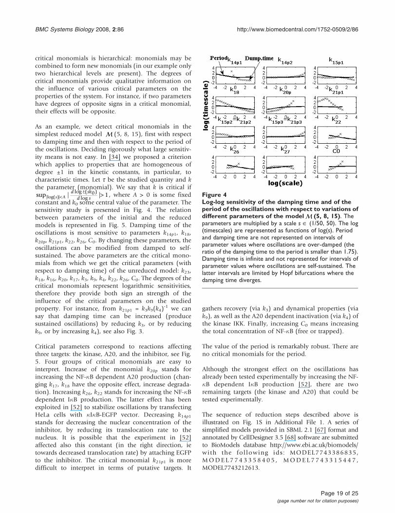
critical monomials is hierarchical: monomials may becombined to form new monomials (in our example onlytwo hierarchical levels are present). The degrees ofcritical monomials provide qualitative information onthe influence of various critical parameters on theproperties of the system. For instance, if two parametershave degrees of opposite signs in a critical monomial,their effects will be opposite.

As an example, we detect critical monomials in thesimplest reduced model (5, 8, 15), first with respectto damping time and then with respect to the period ofthe oscillations. Deciding rigorously what large sensitiv-ity means is not easy. In [34] we proposed a criterionwhich applies to properties that are homogeneous ofdegree ±1 in the kinetic constants, in particular, tocharacteristic times. Let t be the studied quantity and kthe parameter (monomial). We say that k is critical ifsup | ||log( )|

log ( )logs A

d skd s< >t 0 1 , where A > 0 is some fixed

constant and k0 some central value of the parameter. Thesensitivity study is presented in Fig. 4. The relationbetween parameters of the initial and the reducedmodels is represented in Fig. 5. Damping time of theoscillations is most sensitive to parameters k14p1, k18,k20p, k21p1, k22, k26, C0. By changing these parameters, theoscillations can be modified from damped to self-sustained. The above parameters are the critical mono-mials from which we get the critical parameters (withrespect to damping time) of the unreduced model: k23,k18, k16, k20, k17, k3, k9, k4, k22, k26, C0. The degrees of thecritical monomials represent logarithmic sensitivities,therefore they provide both sign an strength of theinfluence of the critical parameters on the studiedproperty. For instance, from k21p1 = k3k9(k4)

-1 we cansay that damping time can be increased (producesustained oscillations) by reducing k3, or by reducingk9, or by increasing k4), see also Fig. 3.

Critical parameters correspond to reactions affectingthree targets: the kinase, A20, and the inhibitor, see Fig.5. Four groups of critical monomials are easy tointerpret. Increase of the monomial k20p stands forincreasing the NF-�B dependent A20 production (chan-ging k17, k18 have the opposite effect, increase degrada-tion). Increasing k26, k22 stands for increasing the NF-�Bdependent I�B production. The latter effect has beenexploited in [52] to stabilize oscillations by transfectingHeLa cells with �I�B-EGFP vector. Decreasing k14p1stands for decreasing the nuclear concentration of theinhibitor, by reducing its translocation rate to thenucleus. It is possible that the experiment in [52]affected also this constant (in the right direction, ietowards decreased translocation rate) by attaching EGFPto the inhibitor. The critical monomial k21p1 is moredifficult to interpret in terms of putative targets. It

gathers recovery (via k3) and dynamical properties (viak9), as well as the A20 dependent inactivation (via k4) ofthe kinase IKK. Finally, increasing C0 means increasingthe total concentration of NF-�B (free or trapped).

The value of the period is remarkably robust. There areno critical monomials for the period.

Although the strongest effect on the oscillations hasalready been tested experimentally by increasing the NF-�B dependent I�B production [52], there are tworemaining targets (the kinase and A20) that could betested experimentally.

The sequence of reduction steps described above isillustrated on Fig. 1S in Additional File 1. A series ofsimplified models provided in SBML 2.1 [67] format andannotated by CellDesigner 3.5 [68] software are submittedto BioModels database http://www.ebi.ac.uk/biomodels/with the fol lowing ids : MODEL7743386835,MODEL 7 7 4 3 3 5 8 4 0 5 , MODEL 7 7 4 3 3 1 5 4 4 7 ,MODEL7743212613.

Figure 4Log-log sensitivity of the damping time and of theperiod of the oscillations with respect to variations ofdifferent parameters of the model (5, 8, 15). Theparameters are multiplied by a scale s Π(1/50, 50). The log(timescales) are represented as functions of log(s). Periodand damping time are not represented on intervals ofparameter values where oscillations are over-damped (theratio of the damping time to the period is smaller than 1.75).Damping time is infinite and not represented for intervals ofparameter values where oscillations are self-sustained. Thelatter intervals are limited by Hopf bifurcations where thedamping time diverges.

BMC Systems Biology 2008, 2:86 http://www.biomedcentral.com/1752-0509/2/86

Page 19 of 25(page number not for citation purposes)

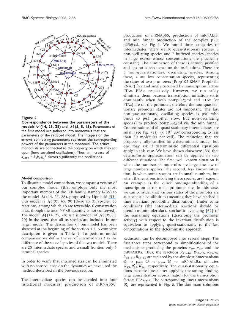
Model comparisonTo illustrate model comparison, we compare a version ofour complex model (that employs only the mostimportant member of the I�B family, namely I�Ba) tothe model (14, 25, 28), proposed by Lipniacki [53].Our model is (39, 65, 90 (there are 39 species, 65reactions, among which 18 are reversible, 6 conservationlaws, though the total NF-�B quantity is not conserved).The model (14, 25, 28) is a submodel of (39,65,90) in the sense that all its species are included in ourlarger model. The description of our model has beensketched at the beginning of the section 3.2. A completedescription is given in Table 1. To perform modelcomparison we define the set of intermediates I as thedifference of the sets of species of the two models. Thereare 25 intermediate species and a small frontier: only 5terminal species.

In order to verify that intermediates can be eliminatedwith no consequence on the dynamics we have used themethod described in the previous section.

The intermediate species can be divided into fourfunctional modules: production of mRNAp50,

production of mRNAp65, production of mRNAI�B,and min funnel production of the complex p50:p65@csl, see Fig 6. We found three categories ofintermediates. There are 10 quasi-stationary species, 3non-oscillating species and 7 buffered species (speciesin large excess whose concentrations are practicallyconstant). The elimination of these is entirely justifiedand has no consequence on the oscillations. There are5 non-quasistationary, oscillating species. Amongthese, 4 are low concentration species, representingthe states of two promoters (Prop105:RNAP, PropIkBa:RNAP) free and singly occupied by transcription factorsFTAx, FTAz, respectively. However, we can safelyeliminate them because transcription initiation startsdominantly when both p50:p65@csl and FTAx (orFTAz) are on the promoter, therefore the non-quasista-tionary promoter states are not important. The lastnon-quasistationary, oscillating species is p50 whobinds to p65 (another slow, but non-oscillatingspecies) to produce p50:p65@csl via the min funnel.Concentrations of all quasi-stationary intermediates aresmall (see Fig. 7a)), (< 10-4 μM corresponding to lessthan 30 molecules per cell). The reduction that wepropose is fully justified for a deterministic model, butone may ask if deterministic differential equationsapply in this case. We have shown elsewhere [33] thatdeterministic approximation can be applied in twodifferent situations. The first, well known situation iswhen the numbers of molecules are large; the law oflarge numbers applies. The second, less known situa-tion, is when some species are in small numbers, butwhen the reactions involving these species are frequent.An example is the quick binding-unbinding of atranscription factor on a promoter site. In this case,we can consider that various states of the promoter areat stochastic equilibrium (meaning they have reached atime invariant probability distribution). Under someconditions (the intermediate reactions should bepseudo-monomolecular), stochastic averaging [69] ofthe remaining equations (describing the promoteractivity) with respect to the invariant distribution isequivalent to applying quasi-stationarity to the fastconcentrations in the deterministic approach.

Reduction can be decomposed into several steps. Thefirst three steps correspond to simplifications of themechanisms producing the proteins p50, p65, and themRNAIkBa. Thus, the reactions R41–46, R32–39, R63–70,R48–51, R55–62 are replaced by the simple submechanismsΔ Æ p65, Δ Æ p50, Δ Æ mRNAIkBa, of rates′ ′ ′R R R45 39 26, , , respectively. The quasi-stationarity equa-

tions become linear after applying the strong binding,large concentration approximation for the transcriptionfactors FTAx-y-z. The corresponding linear mechanisms I are represented in Fig. 6. The dominant solutions

k1

k2

k3k4k5

k6

k7k8

k9

k10

k11

k12

k13

k14

k15

k16

k17

k18

k19

k20

k21k22

k23

k’23

k27

kv

k28

k’28

C0

k22

k14p1

k26

k26

k27

k18

M(14,25,28)

M(5,8,15)

IKK

dep. IkB

degradation

k25

C0

IKK inactivatio

n

IkB degradationA

20pro

duct

ion

A20

deg

rad

ati

on

Co

mp

lex

form

atio

n

Tra

nsp

ort

IkBproduction

k21p1

k14p2

k15p2=k21p2

k20p

kv

Sustained+1

+1

-1+1

-1

+1

+1

-1

+1-1 +1

+1-1

+1

+1 +1 +1

+1

+1

IKK production

Oscillations

k15p3=k21p3

Figure 5Correspondence between the parameters of themodels (14, 25, 28) and (5, 8, 15). Parameters ofthe first model are gathered into monomials that areparameters of the reduced model. The integers on thearrows connecting parameters represent the correspondingpowers of the parameters in the monomial. The criticalmonomials are connected to the property on which they actupon (here sustained oscillations). Thus, an increase ofk21p1 = k2k9 k4

1− favors significantly the oscillations.

BMC Systems Biology 2008, 2:86 http://www.biomedcentral.com/1752-0509/2/86

Page 20 of 25(page number not for citation purposes)

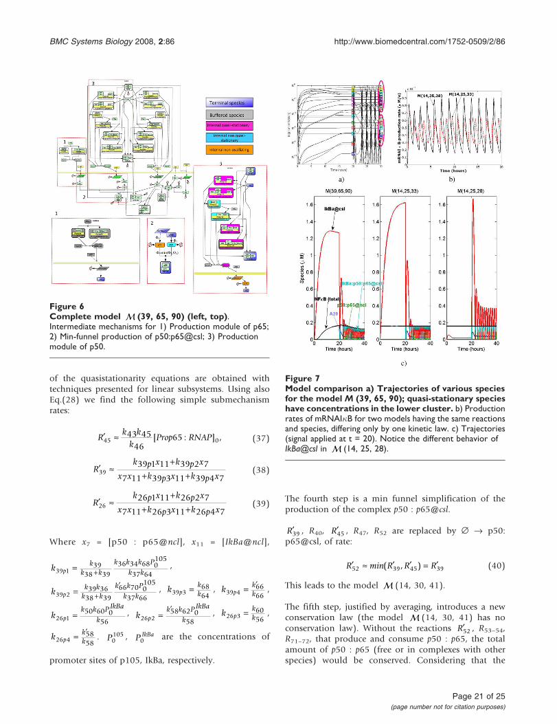
of the quasistationarity equations are obtained withtechniques presented for linear subsystems. Using alsoEq.(28) we find the following simple submechanismrates:

′ ≈Rk k

kProp RNAP45 0

43 4546

65[ : ] , (37)

′ ≈+

+ +R

k p x k p x

x x k p x k p x3939 1 11 39 2 7

7 11 39 3 11 39 4 7(38)

′ ≈+

+ +R

k p x k p x

x x k p x k p x2626 1 11 26 2 7

7 11 26 3 11 26 4 7(39)

Where x7 = [p50 : p65@ncl], x11 = [IkBa@ncl],

k pk

k k

k k k P

k k39 139

38 39

36 34 68 0105

37 64= +

,

k pk k

k k

k k P

k k39 239 36

38 39

66 70 0105

37 66= +

′ , k pkk39 36864

= , k pkk39 46666

= ′,

k pk k P IkBa

k26 150 60 0

56= , k p

k k P IkBa

k26 258 62 0

58=

′ , k pkk26 36056

= ,

k pkk26 45858

= ′. P0

105 , P IkBa0 are the concentrations of

promoter sites of p105, IkBa, respectively.

The fourth step is a min funnel simplification of theproduction of the complex p50 : p65@csl.

′R39 , R40, ′R45 , R47, R52 are replaced by Δ Æ p50:p65@csl, of rate:

′ ≈ ′ ′ = ′R min R R R52 39 45 39( , ) (40)

This leads to the model (14, 30, 41).

The fifth step, justified by averaging, introduces a newconservation law (the model (14, 30, 41) has noconservation law). Without the reactions ′R52 , R53–54,R71–72, that produce and consume p50 : p65, the totalamount of p50 : p65 (free or in complexes with otherspecies) would be conserved. Considering that the

Figure 6Complete model (39, 65, 90) (left, top).Intermediate mechanisms for 1) Production module of p65;2) Min-funnel production of p50:p65@csl; 3) Productionmodule of p50.

Figure 7Model comparison a) Trajectories of various speciesfor the model M (39, 65, 90); quasi-stationary specieshave concentrations in the lower cluster. b) Productionrates of mRNAI�B for two models having the same reactionsand species, differing only by one kinetic law. c) Trajectories(signal applied at t = 20). Notice the different behavior ofIkBa@csl in (14, 25, 28).

BMC Systems Biology 2008, 2:86 http://www.biomedcentral.com/1752-0509/2/86

Page 21 of 25(page number not for citation purposes)

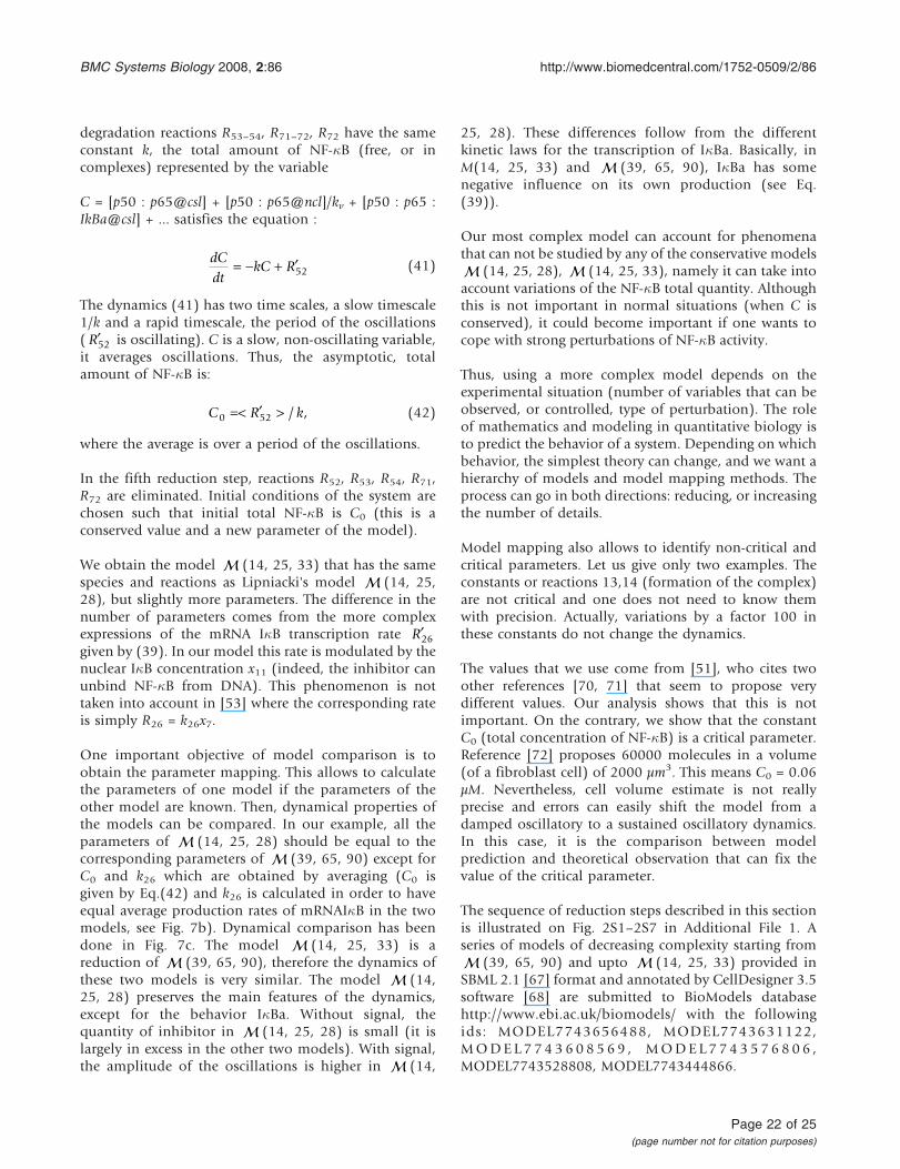
degradation reactions R53–54, R71–72, R72 have the sameconstant k, the total amount of NF-�B (free, or incomplexes) represented by the variable

C = [p50 : p65@csl] + [p50 : p65@ncl]/kv + [p50 : p65 :IkBa@csl] + ... satisfies the equation :

dCdt

kC R= − + ′52 (41)

The dynamics (41) has two time scales, a slow timescale1/k and a rapid timescale, the period of the oscillations( ′R52 is oscillating). C is a slow, non-oscillating variable,it averages oscillations. Thus, the asymptotic, totalamount of NF-�B is:

C R k0 52=< ′ > / , (42)

where the average is over a period of the oscillations.

In the fifth reduction step, reactions R52, R53, R54, R71,R72 are eliminated. Initial conditions of the system arechosen such that initial total NF-�B is C0 (this is aconserved value and a new parameter of the model).

We obtain the model (14, 25, 33) that has the samespecies and reactions as Lipniacki's model (14, 25,28), but slightly more parameters. The difference in thenumber of parameters comes from the more complexexpressions of the mRNA I�B transcription rate ′R26given by (39). In our model this rate is modulated by thenuclear I�B concentration x11 (indeed, the inhibitor canunbind NF-�B from DNA). This phenomenon is nottaken into account in [53] where the corresponding rateis simply R26 = k26x7.

One important objective of model comparison is toobtain the parameter mapping. This allows to calculatethe parameters of one model if the parameters of theother model are known. Then, dynamical properties ofthe models can be compared. In our example, all theparameters of (14, 25, 28) should be equal to thecorresponding parameters of (39, 65, 90) except forC0 and k26 which are obtained by averaging (C0 isgiven by Eq.(42) and k26 is calculated in order to haveequal average production rates of mRNAI�B in the twomodels, see Fig. 7b). Dynamical comparison has beendone in Fig. 7c. The model (14, 25, 33) is areduction of (39, 65, 90), therefore the dynamics ofthese two models is very similar. The model (14,25, 28) preserves the main features of the dynamics,except for the behavior I�Ba. Without signal, thequantity of inhibitor in (14, 25, 28) is small (it islargely in excess in the other two models). With signal,the amplitude of the oscillations is higher in (14,

25, 28). These differences follow from the differentkinetic laws for the transcription of I�Ba. Basically, inM(14, 25, 33) and (39, 65, 90), I�Ba has somenegative influence on its own production (see Eq.(39)).

Our most complex model can account for phenomenathat can not be studied by any of the conservative models (14, 25, 28), (14, 25, 33), namely it can take intoaccount variations of the NF-�B total quantity. Althoughthis is not important in normal situations (when C isconserved), it could become important if one wants tocope with strong perturbations of NF-�B activity.

Thus, using a more complex model depends on theexperimental situation (number of variables that can beobserved, or controlled, type of perturbation). The roleof mathematics and modeling in quantitative biology isto predict the behavior of a system. Depending on whichbehavior, the simplest theory can change, and we want ahierarchy of models and model mapping methods. Theprocess can go in both directions: reducing, or increasingthe number of details.

Model mapping also allows to identify non-critical andcritical parameters. Let us give only two examples. Theconstants or reactions 13,14 (formation of the complex)are not critical and one does not need to know themwith precision. Actually, variations by a factor 100 inthese constants do not change the dynamics.

The values that we use come from [51], who cites twoother references [70, 71] that seem to propose verydifferent values. Our analysis shows that this is notimportant. On the contrary, we show that the constantC0 (total concentration of NF-�B) is a critical parameter.Reference [72] proposes 60000 molecules in a volume(of a fibroblast cell) of 2000 μm3. This means C0 = 0.06μM. Nevertheless, cell volume estimate is not reallyprecise and errors can easily shift the model from adamped oscillatory to a sustained oscillatory dynamics.In this case, it is the comparison between modelprediction and theoretical observation that can fix thevalue of the critical parameter.

The sequence of reduction steps described in this sectionis illustrated on Fig. 2S1–2S7 in Additional File 1. Aseries of models of decreasing complexity starting from (39, 65, 90) and upto (14, 25, 33) provided inSBML 2.1 [67] format and annotated by CellDesigner 3.5software [68] are submitted to BioModels databasehttp://www.ebi.ac.uk/biomodels/ with the followingids: MODEL7743656488, MODEL7743631122,MODEL 7 7 4 3 6 0 8 5 6 9 , MODEL 7 7 4 3 5 7 6 8 0 6 ,MODEL7743528808, MODEL7743444866.

BMC Systems Biology 2008, 2:86 http://www.biomedcentral.com/1752-0509/2/86

Page 22 of 25(page number not for citation purposes)

ConclusionWe have presented a methodology for reducing andcomparing systems biology models. We show how toproduce a hierarchy of coarse grained models that can beused for understanding functioning of the biologicalsystems. We show how models in the hierarchy can bemapped one onto another, thus allowing to decrease orto increase the number of details that are needed for thedescription of the system. Our method identifies the setof critical parameters of the system. This can beparticularly useful for robustness studies (when robust-ness is understood as stability against parametervariability [34]) or for practical multi-target approachesin pharmacology.

We did not approach aspects of multi-scale modelingthat occur in multi-organ physiology, or spatial aspects.Relation with stochastic modelling has been only brieflydiscussed and will be presented in detail elsewhere(Crudu et al., in preparation). The reduction methodspresented here can be applied to systems of biochemicalreactions modeling cell physiology [73] and can beusefully applied to various problems in signalling,metabolism, genetic regulation.

A central idea in our treatment is the hypothesis thatbiological systems are hierarchial, involving manyseparated time scales. The reduction methods wereadapted to exploit this situation (we look for dominantsubsystems, which lead to tremendous simplification).The hierarchical nature of the systems is not sufficientlyexploited by more traditional approaches. For instance,singular perturbation copes with two time scales andeliminates the fastest. In biology, we are often interestedin a "middle" time-scale, corresponding to a particularprocess that we study. We have shown how to eliminateboth faster and slower variables. Another specificity ofsystems biology is the quest for critical parameters. Ourapproach offers naturally a solution: critical parametersare detected in the reduction process. It also extends thetheory of limiting step to complex networks [1]. Showinghow to find critical parameters and dominant simplifica-tions is a first step towards a dynamical systemsapproach to physiology. Indeed, complex networksfulfill various tasks in simple ways by activating a fewdegrees of freedom. Dominant subsystems gather dyna-mical variables that are activated and can change whenthe system needs to perform a given task. Changing taskcould be represented as zooming in and out (change thenumber of degrees of freedom), or jumping laterally(change the set of degrees of freedom) in the hierarchy ofmodels. As pointed out by Denis Noble [74], physiologyshould not be understood from the bottom upwards.Our approach suggests that not only the subjectiveunderstanding, but also the objective functioning of

biological systems can be based on middle-out (meaningvariable level of detail) pictures.

As future work we will improve our algorithms in orderto propose fully automated reduction tools. At present,the automated sections of our methods are the calcula-tion of dominant subsystems of pseudo-monomolecularsubsystems and the calculation of simple sub-mechan-isms stoichiometries and rates. The detection of quasi-stationary and non-oscillating species is semi-auto-mated. The solutions of quasi-stationarity and averagedstationarity equations are not yet fully automated(except for the pseudo-monomolecular case).

We also plan to consider other applications such as highdimensional switches [75].

Concerning our model comparison methods, we wouldlike to study hierarchies of kinetic models coming fromvarious organisms, for which the conserved and thespecific parts are the result of evolution.

Authors' contributionsOR proposed the methodology to reduce nonlinearmodels. AG developed the general theory of multiscalelinear system, together with OR and AZ. AZ and ORdesigned and implemented the algorithms. AL designedthe NF-�B model. All authors drafted, read and approvedthe final manuscript.

Additional material

Additional file 1Hierarchy of NF�B models. This file shows the hierarchy of models usingSystems Biology Graphical Notation (SBGN) and the results of a studyof the truly non-linear reactions.Click here for file[http://www.biomedcentral.com/content/supplementary/1752-0509-2-86-S1.ppt]

AcknowledgementsWe acknowledge support from the French Ministry of Research programACI IMPBio, from the British Council/French Foreign Affairs Ministrycooperation program Alliance (Partenariat Hubert Curien), from theFrench Complex Systems Institute ISC and EC-FP-7 (APO-SYS). AZ ismember of the team "Systems Biology of Cancer "équipe labellisée par laLigue Nationale Contre le Cancer. We thank Upinder Bhalla, Dennis Brayand John Reinitz for inspiring discussions. We also thank the students thatcontributed to some of the programs used in this work: Karine Yviquel,IFSIC intern and Debasis Panda, INRIA intern from IBAB.

References1. Gorban AN and Radulescu O: Dynamic and static limitation in

reaction networks, revisited. Advances in Chemical Engineering2008, 34:103–173 http://arxiv.org/abs/physics/0703278.

2. Lam SH and Goussis DA: The CSP Method for SimplifyingKinetics. International Journal of Chemical Kinetics 1994, 26:461–486.

BMC Systems Biology 2008, 2:86 http://www.biomedcentral.com/1752-0509/2/86

Page 23 of 25(page number not for citation purposes)

3. Chiavazzo E, Gorban AN and Karlin IV: Comparisons of InvariantManifolds for Model Reduction in Chemical Kinetics. CommComp Phys 2007, 2:964–992.

4. Gorban AN and Karlin IV: Method of invariant manifold forchemical kinetics. Chem Eng Sci 2003, 58:4751–4768.

5. Gorban AN and Karlin IV: Invariant manifolds for physical and chemicalkinetics, Lect. Notes. Phys. 660 Berlin, Heidelberg: Springer; 2005.

6. Gorban AN, Karlin IV and Zinovyev AY: Invariant grids forreaction kinetics. Physica A 2004, 333:106–154.

7. Roussel MR and Fraser SJ: On the geometry of transientrelaxation. J Chem Phys 1991, 94:7106–7113.

8. Krauskopf B, Osinga HM, Doedel EJ , Henderson ME,Guckenheimer J, Vladimirsky A, Dellnitz M and Junge O: A surveyof method's for computing (un)stable manifold of vectorfields. International Journal of Bifurcation and Chaos 2005, 15:763–791.

9. Auger P, de la Para RB, Poggiale JC, Sanchez E and Huu TN:Aggregation of variables and applications to populationdynamics. Structured Population Models in Biology and Epidemiology,LNM 1936, Mathematical Biosciences Subseries Berlin: Springer: MagalP, Ruan S 2008, 209–263.

10. Gorban AN, Kazantzis N, Kevrekidis IG, Ottinger HC and Eds: CT:Model Reduction and Coarse-Graining Approaches for MultiscalePhenomena Berlin-Heidelberg-New York: Springer; 2006.

11. Conzelmann H, Saez-Rodriguez J, Sauter T, Bullinger E, Allgower Fand Gilles ED: Reduction of mathematical models of signaltransduction networks: simulation-based approach appliedto EGF receptor signalling. Syst Biol (Stevenage) 2004, 1(1):159–169.

12. Wang R, Zhou T, Jing Z and Chen L: Modelling periodicoscillations of biological systems with multiple timescalesnetwork. Syst Biol 2004, 1:71–84.

13. Indic P, Gurdziel K, Kronauer RE and Klerman EB: Development ofa two-dimension manifold to represent high dimensionmathematical models of the intracellular mammalianclock. J Biol Rhythms 2006, 21:222–232.

14. Borisov NM, Markevich NI, Hoek JB and Kholodenko BN: Signalingthrough Receptors and Scaffolds: Independent InteractionsReduce Combinatorial Complexity. Biophys J 2005, 89:951–966.

15. Conzelmann H, Saez-Rodriguez J, Sauter T, Kholodenko BN andGilles ED: A domain-oriented approach to the reduction ofcombinatorial complexity in signal transduction networks.BMC Bioinformatics 2006, 7:34.

16. Reinhardt V, Winckler M and Lebiedz D: Approximation of slowattracting manifolds in chemical kinetics by trajectory-based optimization approaches. J Phys Chem A 2008,112:1712–1718.

17. Jolliffe IT: Principal Component Analysis, Series: Springer Series inStatistics New York: Springer; 22002, XXIX:.

18. Berkooz G, Holmes P and Lumley JL: The proper orthogonaldecomposition in the analysis of turbulent flows. Annu RevFluid Mech 1993, 25:539–575.

19. Tresser C, Worfolk A and Baas H: Master-slave synchronizationfrom the point of view of global dynamics. Chaos 1995, 5:693–699.

20. Pécou E: Splitting the dynamics of large interaction net-works. J Theor Biol 2005, 232:375–384.

21. Schnell S and Maini PK: Enzyme Kinetics Far From theStandard Quasi-Steady-State and Equilibrium Approxima-tions. Mathematical and Computer Modelling 2002, 35:137–144.

22. Bogoliubov NN and Mitropolski YA: Asymptotic Methods in the Theoryof Nonlinear Oscillations New York: Gordon and Breach; 1961.

23. Givon D, Kupferman R and Stuart A: Extracting macroscopicdynamics: model problems and algorithms. Nonlinearity 2004,17:R55–R127.

24. Acharya A and Sawant A: On a computational approach for theapproximate dynamics of averaged variables in nonlinearODE systems: Toward the derivation of constitutive laws ofthe rate type. J Mech Phys Sol 2006, 54:2183–2213.

25. Toth J, Li G, Rabitz H and Tomlin AS: The Effect of Lumping andExpanding on Kinetic Differential Equations. SIAM J Appl Math1997, 57:1531–1556.

26. Clarke BL: General Method for Simplifying Chemical Net-works while Preserving Overall Stoichiometry in ReducedMechanisms. J Phys Chem 1992, 97:4066–4071.

27. Kruskal MD: Asymptotology. Mathematical Models in PhysicalSciences New Jersey: Prentice-Hall: Dobrot S 1963, 17–48.

28. Holmes MH: Introduction to Perturbation Methods New York: Springer;1995.

29. Vishik MI and Ljusternik LA: Solution of some perturbationproblems in the case of matrices and self-adjoint or non-selfadjoint differential equations. Russian Math Surveys 1960,15:1–73.

30. Akian M, Bapat R and Gaubert S:Min-plus methods in eigenvalueperturbation theory and generalised Lidskii-Vishik-Ljuster-nik theorem. arXiv e-print math.SP/0402090 2004.

31. White RB: Asymptotic Analysis of Differential Equations London:Imperial College Press and World Scientific; 2006.

32. Ball K, Kurtz TG, Popovic L and Rempala G: Asymptotic analysisof multiscale approximations to reaction networks. Ann ApplProbab 2006, 16:1925–1961.

33. Radulescu O, Muller A and Crudu A: Théorémes limites pourdes processus de Markov à sauts. Synthèse des resultats etapplications en biologie moleculaire. Technique et ScienceInformatique 2007, 26:443–469 http://cat.inist.fr/?aModele=affi-cheN&cpsidt=18842024.

34. Gorban AN and Radulescu O: Dynamical robustness ofbiological networks with hierarchical distribution of timescales. IET Systems Biology 2007, 1:238–246.

35. Glass L: Classification of biological networks by theirqualitative dynamics. J Theor Biol 1975, 54:85–107.

36. Snoussi EH: Qualitative dynamics of piecewise-linear differ-ential equations: a discrete mapping approach. Dyn Stab Syst1989, 4:189–207.

37. de Jong H, Gouzé JL, Hernandez C, Page M, Sari T and Geiselmann J:Qualitative simulation of genetic regulatory networks usingpiecewise-linear models. Bull Math Biol 2004, 66:301–340.

38. Klamt S, Saez-Rodriguez J, Lindquist JA, Simeoni L and Gilles ED: Amethodology for the structural and functional analysis ofsignaling and regulatory networks. BMC Bioinformatics 2006,7:56.

39. Temkin ON, Zeigarnik AV and Bonchev D: Chemical ReactionsNetworks Boca Raton: CRC Press; 1996.

40. Tikhonov AN, Vasileva AB and Sveshnikov AG: Differential equationsBerlin: Springer; 1985.

41. Wasow W: Asymptotic Expansions for Ordinary Differential EquationsNew York: Wiley; 1965.

42. Fenichel N: Geometric Singular Perturbation Theory forOrdinary Differential Equations. J Diff Eq 1979, 31:53–98.

43. Gagneur J and Klamt S: Computation of elementary modes: aunifying framework and the new binary approach. BMCBioinformatics 2004, 5:175.

44. Urbanczik R and Wagner C: An improved algorithm forstoichiometric network analysis: theory and applications.Bioinformatics 2005, 21:1203–1210.

45. Klamt S, Gagneur J and von Kamp A: Algorithmic approaches forcomputing elementary modes in large biochemical reactionnetworks. IEE Proc Syst Biol 2005, 152:249–55.

46. Bjorner A, Las Vergnas M, Sturmfels B, White N and Ziegler G:Oriented Matroids Cambridge: Cambridge University Press; 21999.

47. Bruno AD: Power Geometry in Algebraic and Differential EquationsAmsterdam: North-Holland; 2000.

48. Pontryagin LS and Rodygin LV: Approximate solution of asystem of ordinary differential equations involving a smallparameter in the derivatives. Soviet Math Dokl 1960, 1:237–240.

49. Sari T and Yadi K: On Pontryagin-Rodygin's theorem forconvergence of solutions of slow and fast systems. Electr J DiffEq 2004, 2004:1–17.

50. Ghosh S and Karin M: Missing pieces in the NF-�B puzzle. Cell2002, 109:S81–96.

51. Hoffmann A, et al: The I�B-NF-�B signaling module: temporalcontrol and selective gene activation. Science 2002, 298:1241–1245.

52. Nelson DE, et al: Oscillations in NF-�B Signaling Control theDynamics of Gene Expression. Science 2004, 306:704–708.

53. Lipniacki T, Paszek P, Brasier AR, Luxon B and Kimmel M:Mathematical model of NF-�B regulatory module. J TheorBiol 2004, 228:195–215.

54. Ihekwaba AEC, et al: Sensitivity analysis of parameters con-trolling oscillatory signalling in the NF-�B pathway: theroles of IKK and I�Ba. Syst Biol 2004, 1:93–102.

55. Krishna S, Jensen M and Sneppen K: Minimal model of spikyoscillations in NF-�B signaling. Proc Natl Acad Sci USA 2006,103:10840–45.

56. Yean D and Gralla J: Transcription reinitiation rate: a specialrole for the TATA box. Mol Cell Biol 1997, 17:3809–16.

57. Yie J, Senger K and Thanos D: Mechanism by which the IFN-benhanceosome activates transcription. Proc Natl Acad Sci USA1999, 96:13108–13.

BMC Systems Biology 2008, 2:86 http://www.biomedcentral.com/1752-0509/2/86

Page 24 of 25(page number not for citation purposes)

58. Dintzis HM: Assembly of the peptide chains of hemoglobin.Proc Natl Acad Sci USA 1961, 47:247–61.

59. Jansen GMC and Moller W: Kinetic studies on the role ofelongation factors 1b and 1g in protein synthesis. J Biol Chem1988, 263:1773–8.

60. Narayan S, Widen SG, Beard WA and Wilson SH: RNApolymerase II transcription. J Biol Chem 1994, 269:12755–63.

61. Wen JD, Lancaster L, Hodges C, Zeri AC, Yoshimura SG, Noller HF,Bustamante C and Tinoco I: Following translation by singleribosomes one codon at a time. Nature 2008, 452:598–603.

62. Hart DJ, Speight RE, Cooper MA, Sutherland JD and Blackburn JM:The salt dependence of DNA recognition by NF-�B p50: adetailed kinetic analysis of the effects on affinity andspecificity. Nucl Acids Res 1999, 27:1063–9.

63. de Lumley M, Hart DJ, Cooper MA, Symeonides S and Blackburn JM:A biophysical characterisation of factors controlling dimer-isation and selectivity in the NF-�B and NFAT families. J MolBiol 2004, 339:1059–75.

64. Phelps CB, Sengchanthalangsy LL, Huxford T and Ghosh G:Mechanism of I�Ba binding to NF-�B dimers. J Biol Chem2000, 275:29840–6.

65. O'Dea E, Barken D, Peralta R, Tran T, Werner S, Kearns J,Levchenko A and Hoffmann A: A homeostatic model of I�Bmetabolism to control constitutive NF-�B activity. Mol SystBiol 2007, 3:1–7.

66. Rabitz H, Kramer M and Dacol D: Sensitivity analysis inchemical kinetics. Annual Review of Physical Chemistry 1983,34:419–461.

67. Hucka M, Finney A, Sauro HM, Bolouri H, Doyle J, Kitano H,Arkin AP, Bornstein BJ and Bray D, et al: The systems biologymarkup language (SBML): a medium for representation andexchange of biochemical network models. Bioinformatics 2003,19:524–531.

68. Funahashi A, Tanimura N, Morohashi M and Kitano H: CellDe-signer: a process diagram editor for gene-regulatory andbiochemical networks. BIOSILICO 2003, 1:159–162.

69. Freidlin M and Wentzell A: Random perturbations of dynamical systemsNew York: Spinger; 1984.

70. Malek S, Huxford T and Ghosh G: I�B Functions through DiectContacts with the Nuclear Localization Signal and the DNABinding Sequences of NF-�B. J Biol Chem 1998, 273:25427–25435.

71. Carlotti F, Dower SK and Qwarnstrom EE: Dynamic Shuttling ofNuclear Factor �B between the Nucleus and Cytoplasm as aConsequence of Inhibitor Dissociation. J Biol Chem 2000,273:41028–41034.

72. Carlotti F, Chapman R, Dower SK and Qwarnstrom EE: Activationof nuclear factor �B in single living cells. J Biol Chem 1999,274:37941–37949.

73. Bray D: Protein molecules as computational elements inliving cells. Nature 1995, 376:307–312.

74. Noble D: The Rise of Computational Biology. Nature ReviewsMolecular Cell Bioloy 2002, 3:460–463.

75. Bhalla US, Ram PT and Iyengar R: MAP Kinase Phosphatase as aLocus of Flexibility in a Mitogen-Activated Protein KinaseSignaling Network. Science 2002, 297:1018–1023.

76. Calzone L, Gelay A, Zinovyev A, Radvanyi F and Barillot E: Acomprehensive modular map of molecular interactions inRB/E2F pathway. Molecular Systems Biology 2008, 4:174.

Publish with BioMed Central and every scientist can read your work free of charge

"BioMed Central will be the most significant development for disseminating the results of biomedical research in our lifetime."

Sir Paul Nurse, Cancer Research UK

Your research papers will be:

available free of charge to the entire biomedical community

peer reviewed and published immediately upon acceptance

cited in PubMed and archived on PubMed Central

yours — you keep the copyright

Submit your manuscript here:http://www.biomedcentral.com/info/publishing_adv.asp

BioMedcentral

BMC Systems Biology 2008, 2:86 http://www.biomedcentral.com/1752-0509/2/86

Page 25 of 25(page number not for citation purposes)