Robust reconstruction of the discrete state for a class of nonlinear uncertain switched systems

1

Robust reconstruction of the discrete state for a classof nonlinear uncertain switched systemsN. Orani, A. Pisano, M. Franceschelli, A. Giua and E. Usai

Abstract

This paper presents an approach to the robust state reconstruction for a class of nonlinear switchedsystems affected by model uncertainties. Under the assumption that the continuous state is available formeasurement, an approach is presented based on concepts and methodologies derived from the slidingmode control theory. The time needed for reconstructing the discrete state after a transition can be madearbitrarily small by sufficiently increasing a certain observer tuning parameter.

Published as:N. Orani, A. Pisano, M. Franceschelli, A. Giua and E. Usai, ”Robust reconstruction of the discretestate for a class of nonlinear uncertain switched systems” 3rd IFAC Conference on Analysis andDesign of Hybrid Systems, (Zaragoza, Spain), Sep. 2009.

The authors are with the Department of Electrical and Electronic Engineering (DIEE), University of Cagliari,P.zza d’Armi,I-09123, Cagliari, Italy. emails: {n.orani,pisano}@diee.unica.it

DRAFT

2

I. INTRODUCTION

In the last decade the control community has devoted a great deal of attention to the studyof switched systems. A switched system has a discrete dynamics represented by a finite statemachine that evolves according to the occurrence of discrete events. To each discrete state (or“mode”) a continuous dynamics is associated [16], [6], [5], [7], [17], [1].

A problem of great interest is the reconstruction of the discrete-state through the observationof measurable system outputs. The techniques developed in this framework can be applied toseveral problems where the discrete events are not observable. In the framework of discrete eventsystems, several approaches have been proposed to estimate the discrete state [10], [11]. In amore general hybrid context, the discrete state estimation has been discussed in [13], [14].

In a recent work [2], the problem of invertibility of nonlinear systems [12] was addressed forthe class of switched nonlinear systems affine in the control variables. In general the problem ofinvertibility for switched systems, especially linear switched systems, has received considerableattention [4], [3], [15], [9]. In this paper we investigate the problem of the discrete statereconstruction for switched systems building on the idea that a general class of switched systemscan be modeled by nonlinear systems with an affine boolean input representing the systemdiscrete state.

Objective of the present work is to reconstruct such a boolean input despite bounded uncer-tainties affecting the system dynamics.

We propose a sliding mode based technique by relying on the remarkable properties ofrobustness against uncertainties and disturbances featured by such an approach [26]. We referto the theoretical framework of the observers for systems with unknown inputs. Sliding modeobservers offer the opportunity of reconstructing the unmeasurable quantities affecting the systemdynamics, which can be exploited to solve the problem addressed in this work.

The organization of the paper is as follows. Section II describes the considered class ofuncertain switched systems. It is pointed out, in particular, that the considered class, that embedsboth analog and boolean terms, can capture switched dynamics of a certain degree of generality.Section III presents the proposed discrete state reconstruction scheme which is based on thesecond-order sliding mode (2-SM) approach. Section IV introduces a case study of a physicalexample (an hydraulic three-tank system) that falls into the considered class of switched systems.Section V deals with the simulation results and the final Section VI summarizes the attainedresults and draws possible lines for future improvements of the presented results.

II. PROBLEM FORMULATION

In this paper we examine the class of switched systems that can be represented in the form:

x(t) = G(x,u, t)+D(x,u, t)δ (σ(t))+ ε(x, t) (1)

where x(t) ∈Rn is the continuous state, u(t) ∈Rp is the input to the system, G(x,u, t) ∈Rn andD(x,u, t) ∈ Rn×L are known vector fields, and ε(x, t) ∈ Rn is an uncertain term that representspossible sources of uncertainties such as modelling errors and/or external disturbances.

DRAFT

3

The piecewise-constant integer function σ(t) ∈ {0, . . . ,k−1} represents the discrete state ofsystem (1). Vector δ (σ(t)) ∈ {0,1}L contains boolean elements. It maps the discrete state σ(t)into an L-dimensional boolean vector which “encodes” the actual discrete state.

Model (1) can represent switched systems with, at most, k ≤ 2L different dynamics. Theproblem tackled in this paper is the reconstruction of the discrete state σ(t).

A. Assumptions

We now specify the assumptions which are met about the considered class of systems (1).The continuous state x(t) is supposed to be fully measurable, and G(x,u, t), D(x,u, t) are

supposed to be known.The dimension L of vector δ (t) must not exceed the dimension of the continuous state:

L≤ n (2)

The boolean vector δ (t) is not available due to the uncertainty in the discrete state. Thediscrete state σ(t) can be uniquely recovered from the boolean vector δ (t), and viceversa.

Let the time evolutions of the continuous state x and exogenous input u variables be a-prioriconfined in the compact domains X and U.

As for the matrix field D(x,u, t), let it be norm-bounded and smooth in the domain X×Uuniformly in time so that two constants D0 and D1 exist such that

‖D(x,u, t)‖ ≤ D0 ‖D(x,u, t)‖ ≤ D1 (3)

D(x,u, t) is also assumed to be full rank which implies that a constant D2 exists such that

‖[DT (x,u, t)D(x,u, t)]−1DT (x,u, t)‖ ≥ D2 (4)

As for the unmeasurable state-dependent uncertainty/disturbance term ε(x, t), let it be uni-formly norm-bounded and smooth in the domain X so that two constants ε0 and ε1 exist suchthat

‖ε(x, t)‖ ≤ ε0 ‖ε(x, t)‖ ≤ ε1 (5)

Note that no boundedness or smoothing requirements are met on the vector field G(x,u, t).

B. Comments on the considered class of systems

We now show that the considered class of switched systems (1) is general enough to representthe following continuous-time switched nonlinear dynamics

x(t) = Gσ(t)(x,u, t)+ ε(x, t) (6)

where σ(t) ∈ {0, . . . ,k− 1} is the discrete state. A simple systematic procedure to put system(6) into the form (1) is now given.

Define the matrices D(x,u, t) and G(x,u, t) as follows (omitting the dependence of its entriesfrom x,u and t)

D(x,u, t) =[

G1−G0 G2−G0 · · · Gk−1−G0]

G(x,u, t) = G0(x,u, t)(7)

DRAFT

4

and letδ (σ(t)) = [δ1(σ(t)),δ2(σ(t)), ...,δL(σ(t))]T (8)

where

δ j(σ(t)) ={

1 if j = σ(t) j = 1,2, ...,L0 otherwise

(9)

One can readily verify that system (6) is equivalent to (1),(7)-(9), whose main characteristicsis that of being affine in the boolean vector δ (σ(t)) defining the current mode of operation. Thusthe considered class (1) is capable of representing nonlinear switched systems with significantdegree of generality.

III. DISCRETE STATE OBSERVER DESIGN

The proposed discrete state estimator (which assumes the knowledge of the continuous systemstate) takes the following form:

z = G(x,u, t)+w(t) (10)

where z represents the observer state and w is an observer input to be designed. Let e = x− zbe the observer error variable. Then, from (1) and (10), the observer error dynamics is

e = D(x,u, t)δ (t)+ ε(x, t)−w(t) (11)

A. Observer input design

Our objective is to design an observer control vector w guaranteeing the finite-time conver-gence to zero of e and e.

In [24], within a distinct framework related to a fault detection and insulation problem, anapproach to unknown input reconstruction was suggested based on standard first-order slidingmode control technique [26]. Such an approach could be used to reconstruct the discrete state ofthe switched systems using the equivalent control principle through low pass filtering. However,it is well known that the methods based on low pass filtering are intrinsically approximatemethods [26] which can guarantee, at best, the asymptotic reconstruction of the discrete systemstate [23]-[24].

Here we propose a different approach based on second-order sliding modes that enables us toreconstruct the discrete state without any filtering, therefore leading to a solution convergingin finite time and theoretically exact.Consider the second time derivative of the error variable e

e = D(x,u, t)δ (t)+Dddt

δ (t)− ε(x, t)− w(t) (12)

which can be rewritten in compact form as follows:

e = ϕ(x,u, t)− w(t) (13)

The uncertain “drift term” ϕ(·) = [ϕ1(·),ϕ2(·), ...,ϕn(·)]T takes the following form

DRAFT

5

ϕ(x,u, t) = D(x,u, t)δ (t)+Dddt

δ (t)− ε(x, t) (14)

which is affected by the unmeasurable vector of boolean elements δ (t) that must be reconstructed.Note that the time derivative of the observer input vector w(t) appears in (13). Denote v(t) =[v1,v2, ...,vn]T ≡−w(t) and

yi,1 = ei

yi,2 = ei(15)

where ei and ei represent the i-th entry of vectors e and e. Then it is possible to rewrite system(13) in terms of n de-coupled single input subsystems having the following form

{yi,1 = yi,2, i = 1,2, ..,nyi,2 = ϕ i(x,u, t)+ vi

(16)

The problem is to find a set of control inputs vi stabilizing the uncertain SISO systems (16) infinite time. To solve this problem, the second-order sliding mode control approach [25] appearsto be particularly appropriate because of systems (16) have relative degree two with respect tothe inputs vi’s which are treated as auxiliary control variables. The control task is complicatedby the two issues: (a) variables yi,2 (i = 1,2, ...,n) are not measurable, and (b) the drift termsϕ i(x,u, t) are uncertain.

The boundedness properties of the drift terms ϕ i(x,u, t) play a crucial role and critically affectthe solution to the control problem. In [19] the problem was solved under the condition that aconstant upperbound Φi to the drift term magnitude can be computed

|ϕ i(x,u, t)| ≤Φi ∀t (17)

Denote as ti (i = 1,2, ...) switching instants at which the active dynamics is commuting. Thediscrete state σ(t), and then also the vector δ (t), are piecewise constant during the time intervalsTi = (ti, ti+1) between two adjacent mode switchings. This means that the time derivative d

dt δ (t)is identically zero during the time intervals Ti between two adjacent mode switching, and featurean impulsive behaviour at the switching instants ti.

The effect of the impulsive ddt δ (t) term is a jump in the e− e state trajectories of system (13).

More precisely, as it is clear from (11), the e trajectories will be discontinuous at the switchinginstants, while the e trajectories will be continuous.

Let the mode switching sequence of the hybrid dynamics have a dwell time td . This meansthat ti+1− ti ≥ td , for i≥ 0.

The main idea is to use the discontinuous controller in [19]. Under the condition (17), suchcontroller is able to stabilize the uncertain SISO systems (16) in a finite time t∗ << td startingfrom any initial conditions e(0) = e0, e(0) = e0, with ‖e0‖ and ‖e0‖ upper bounded by arbitrarilylarge constants. Thus, at any time t ∈ [t∗, t1) the conditions e(t) = e(t) = 0 will be satisfied.

The state jumps occurring at the switching instants ti (i = 1,2, ...) where the vector δ (t) isundergoing a discontinuity, will have the main effect of setting new nonzero initial conditionsfor e(t+i ).

DRAFT

6

So, at the first switching instants t1 the system (16) will leave the origin according to e(t+1 ) = et1with ‖et1‖ ≤ ‖D(x,u, t)‖‖δ (t)‖ ≤ D0

√n (the norm of the boolean vector δ will never exceed

the value√

n).After a new transient whose duration can be made less than t∗ the system will be steered back

to the origin. Thus, at any time t ∈ [t1 +t∗, t2) the conditions e(t) = e(t) = 0 will be satisfied. Thereasoning is repeated over all the successive switching intervals. The key point is the capabilityof the robust controller presented in [19], that will be specified in the sequel, of steering to zerothe SISO systems (16) arbitrarily fast during the time interval between two adjacent modeswitchings.

Along any interval Ti ≡ (ti−1, ti), (i = 1,2, ...), t0 ≡ 0, the drift term ϕ(x,u, t) is

ϕ(x,u, t) = D(x,u, t)δ (t)− ε(x, t) t ∈ (ti−1, ti) (18)

which can be upper bounded in the form

‖ϕ(x,u, t)‖ ≤ Φ≡ D1√

n+ ε1, t ∈ (ti−1, ti) (19)

The existence of such a constant upper bound allows for the possibility to design a robustcontroller featuring the desired finite time convergence properties. Next theorem outlines themain result by introducing the so-called “Suboptimal” second-order sliding mode control algo-rithm [19], [25], [22], together with the tuning rules that allow to obtain an arbitrarily fastconvergence, which is a basic requirement of the present problem.

Theorem 1: Consider system (16) and the control law

vi(t) =−VM sign(yi,1(t)− 1

2yi,1(ξi, j))

ξi, j ≤ t < ξi, j+1j = 1,2, ...

(20)

where ξi,0 = t0 ≡ 0, ξi, j is the sequence of time instants at which yi,2(t) = 0, and

VM = ΓΦ (21)

Denote the sequence of the switching instants as th, h = 1,2, .... Then there is Γ∗ such that, forany Γ≥ Γ∗, the following conditions are provided.

yi,1(t) = yi,2(t) = 0, t ∈ (th + t∗, th+1). (22)

where i = 1,2, ...,n and with t∗ being arbitrarily small.

Proof of Theorem 1 The proof exploits the basic convergence properties of the suboptimalsecond-order sliding mode control algorithm [25], [22]. During the first switching interval [0, t1)the suggested algorithm provides for the attainment of condition (22) with a transient time t∗

fulfilling the next inequality [19], [25]

t∗ ≤ |yi,1(0)|+ |yi,2(0)|g(Γ;Φ)

(23)

where g(Γ;Φ) is a function such that

limΓ→∞g(Γ;Φ) = ∞ ∀Φ (24)

DRAFT

7

On the basis of the boundedness assumptions outlined in the Section II.A, there exist constantbound to ‖e(0)‖ and ‖e(0)‖. Then, by choosing Γ sufficiently large one can guarantee thatt∗ << td .

At t = t1, at which the yi,1 and yi,2 variables are all zero, vector e undergoes a jump such that

‖e(t+1 )‖ ≤ ‖D(x,u, t)‖‖δ (t)‖ ≤ D0√

n (25)

It then starts a new transient with the new initial conditions yi,1(t+1 ) = 0, and yi,2(t+1 ) such that|yi,2(t+1 )| ≤ D0 (the square root of n does not appear when a specific value of i is considered).The time needed for steering the system back to the origin is then bounded by a relationshipsimilar to (23) but with different error initial conditions as follows

t∗ ≤ D0

g(Γ;Φ)(26)

Considering (26) it is possible to select Γ sufficiently large to make t∗ << td , which meansthat the following condition will be achieved during the second switching interval t ∈ (t1, t2)

yi,1(t) = yi,2(t) = 0, t ∈ (t1 + t∗, t2). (27)

By iterating the same reasoning it is proven that the proposed controller is able to guaranteethe attainment of conditions (22) with the transient time t∗ << td that can be made arbitrarilysmall by taking the observer gain parameter Γ sufficiently large, which concludes the proof. ¤

B. Discrete state reconstruction

It was shown in the previous Section that there is t∗ such that, in every “inter-switching”interval Ti ≡ (ti−1, ti) the next conditions hold

e = e = 0, t ∈ [ti−1 + t∗, ti) (28)

From the definition (11) of e, its zeroing implies that

D(x,u, t)δ (t)+ ε(x, t)−w(t) = 0 (29)

Notice that the observer input w(t) is obtained integrating the discontinuous signal v(t), whosesign switches at very high (theoretically infinite) frequency (Zeno behaviour), then w(t) is acontinuous signal.

By neglecting the uncertainty ε(x, t) in (29) it yields naturally the following reconstructionformula that defines a “non-thresholded” estimate of the boolean vector δ .

δ (t) = [DT (x,u, t)D(x,u, t)]−1DT (x,u, t)w(t) (30)

The non-thresholded estimate is not robust against the uncertainty ε(x, t). By (29), the esti-mation error δ (t)−δ (t) will be such that

‖δ (t)−δ (t)‖ ≤ ‖[DT (x,u, t)D(x,u, t)]−1DT (x,u, t)‖‖ε‖(31)

DRAFT

8

It can be fruitfully exploited the boolean nature of the vector δ (t) by introducing a thresh-olding that rounds the value of δ (t) to the closest integer value between 0 and 1. It yields the“thresholded” estimate δ (t) defined according to

δi(t) ={

1 δi(t) > 0.50 δi(t)≤ 0.5

(32)

where δi(t) and δi(t) are the i-th entries of vectors δ (t) and δ (t) respectively.The thresholded estimate results to be robust against any error (δi(t)−δi) less, in magnitude,

than 0.5. Thus it can be explicitly given a bound to the maximal tolerated magnitude for theuncertainty term.

From the requirement that ‖δ (t)−δ (t)‖≤ 0.5 it yields by (31), (4), (5) the following maximalacceptable bound for the norm of the uncertainty term

‖ε(x, t)‖ ≤ ε0 ≤ 0.5D2

(33)

The fulfillment of (33) guarantees the insensitivity of the estimate δ against the uncertainty,namely the condition

δ (t) = δ (t), t ∈ [ti−1 + t∗, ti), i = 1,2, ... (34)

Lemma 1 Under the condition that the norm of the uncertain term ε(x, t) fulfills the restriction(33), the proposed estimation procedure given by (30), (32) provides the exact reconstructionof the boolean vector δ in the time intervals t ∈ [ti−1 + t∗, ti), according to (34)

Remark 1 The requirement of providing the observer convergence within the arbitrarily smalltransient time t∗ << td would correspond, in the linear context, to locate the eigenvalues of theerror dynamics far away from the origin. Generally, this strongly deteriorate the robustnessagainst the measurement noise of the resulting linear “high gain” observer. It can be argued,due to the analysis made in [20], [21], that the magnification of the noise in the considered2-SMC observer could be less severe than in the linear observer counterpart. This topic will beaddressed in more detail in next research activities.

IV. THE THREE-TANK SYSTEM CASE STUDY

The three-tank water process is regarded as a valuable setup for investigating nonlinearmultivariable control as well as fault diagnosis schemes [27]. Let us show that it can be modelledas a switched affine system according to the general formulation (1).

The vertical multi-tank system that we shall consider is composed of three tanks of differentshape interconnected as shown in Fig. 1, a water inflow q(t) that supplies the upper tank n.1 and three on-off valves V 1sw,V 2sw,V 3sw that determine whether an outflow from each Tankexists or not. The on-off state of the three valves define the 8 possible operating mode of theconsidered system.

Refer to the schematic representation in Fig. 1. Signal q(t), the inflow to the upper tank,represent a measurable input to the system, the binary signals U1,U2 and U3 are the unknown

DRAFT

9

states of the on-off valves, and H1,H2 and H3 are the water levels which represent the continuousstate of the three-tank system. It is the objective of the present work to present a scheme forreconstructing the states of the three on-off valves by assuming the knowledge of the waterlevels and of the input inflow q(t) to the upper tank.

Fig. 1. System inputs and outputs

Let us model the three tank system. The flow balance equations lead to

V1 = q(t)−C1(t)√

H1 (35)

V2 = C1(t)√

H1−C2(t)√

H2 (36)

V3 = C2(t)√

H2−C3(t)√

H3 (37)

where V1,V2,V3 correspond to the actual volume of water in the three tanks and C1(t),C2(t),C3(t)are nonnegative coefficients. Due to the on-off nature of the valves, the Ci(t) coefficients (i =1,2,3) can assume two values only according to

Ci(t) ={

0 when valve Visw is OFFC∗i when valve Visw is ON

(38)

DRAFT

10

Let us define three boolean variables U1(t),U2(t),U3(t) representing the status of the three valves,so that the Ci(t) terms can be rewritten as

Ci(t) = C∗i Ui(t) (39)

Further, the following simple relationships holds

Vi = βi(Hi)Hi, i = 1,2,3 (40)

where βi(Hi) (i = 1,2,3) represents the cross sectional area of the i− th tank i at the levelheight Hi.

It yields the simple model

H1 = 1β1(H1)

[q(t)−C∗1

√H1U1(t)

](41)

H2 = 1β2(H2)

[C∗1√

H1U1(t)−C∗2√

H2U2(t)]

(42)

H3 = 1β3(H3)

[C∗2√

H2U2(t)−C∗3√

H3U3(t)]

(43)

Collecting into a boolean vector the discrete states of the on-off valves as follows

δ (t) = [U1(t),U2(t),U3(t)]T ∈ {0,1}3 (44)

it is straightforward to rewrite the model (41)-(43) in the form (1) with x = [H1,H2,H3]T , u = q(t)and

G(x,u, t) =

q(t)β1(H1)

00

(45)

D(x,u, t) =

−C1

∗√H1β1(H1)

0 0C1∗√H1

β2(H2)−C2

∗√H2β2(H2)

0

0 C2∗√H2

β3(H3)−C3

∗√H3β3(H3)

(46)

According to the notation introduced in section II, it must be highlighted that in our case aparticular instance for (44) represent one of the possible k = 8 discrete states σ(t) in witch thethree-tank system could be found.

In the derived three tank system the dimension L of vector δ (t) is L = 3 which does notexceed the dimension n = 3 of the continuous state, as required in assumption (2).

The assumptions (3) on the matrix D(x,u, t) are trivially satisfied if the water levels H1(t),H2(t),H3(t)remains strictly positive during the observation process. Further the assumption (4) requires thatthe square matrix D(x,u, t) is nonsingular. Since

detD(x,u, t) =− C1∗C2

∗C3∗

β1(H1)β2(H2)β3(H3)

√H1H2H3 (47)

again the assumption (4) is fulfilled if none of the water levels become zero during theobservation process. Assuming that an appropriate closed-loop supervisory system has been

DRAFT

11

designed, capable of guaranteeing that Hi(t) ≥ H∗i > 0, i = 1,2,3, the proposed observer can

provide for the reconstruction of the binary signal vector δ (t).An additive error term ε(x, t) may take into account possible discrepancies between the actual

and nominal system model as well as possible external disturbances. It is stated in the Lemma1 that the discrete state can be still reconstructed exactly provided that the norm of ε(x, t) issufficiently small.

It is worth noting that the discrete state σ(t) ∈ {0,1, · · · ,7} can be reconstructed from thethresholded estimates δ1(t), δ2(t), δ3(t) by means of the following expression

σ(t) = δ1(t) ·22 + δ2(t) ·21 + δ3(t) ·20 (48)

V. SIMULATION RESULTS

The effectiveness of the suggested discrete state observer is now studied by means of somesimulative analysis conducted on the three tank model (41)−(43). The inflow input q(t) and thebinary state δ (t) have been selected in such a way that the tanks never become empties, thatwould cause the loss of observability for the system.

The cross-sectional area functions β1(H1),β2(H2),β3(H3) have the following analytical ex-pressions which depends on the particular, different, shapes for the considered three tank systemrepresented in Figure 1:

β1(H1) = aw

β2(H2) = cw+bwH2

β3(H3) = w√

R2− (R−H3)2

where a,b,c,w,R are appropriate constant geometric parameters. The parameter values used inthe simulations are reported in the Table 1. Euler integration method with the fixed samplingtime Ts = 0.001s has been used.

TABLE ITABLE 1. PARAMETERS OF THE TREE TANK SYSTEM

Parameter Value Unit

C1∗ 4.702∗10−5 m3

hC2∗ 4.49∗10−5 m3

hC3∗ 4.51∗10−5 m3

hα1 0.28a 0.035 mw 0.035 mb 0.348 mc 0.1 mR 0.365 m

A disturbance vector with elements of the form

εi(x, t) = 0.1(|H1(t)|+ |H2(t)|+ |H3(t)|)sin(ωt), i = 1,2,3 (49)

DRAFT

12

is considered, and a band-limited additive white noise is added to the level measurementsH1,H2,H3. The binary signal inputs U1(t),U2(t),U3(t) defining the discrete state of the systemhave been selected as shown in the plot of the next figure 2 (the same profile for all the simulationtests has been used). It can be noted that a dwell time of 0.5s has been used.

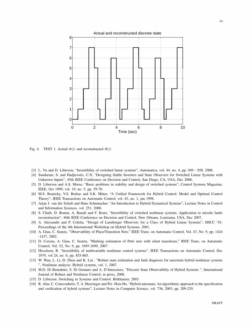
In the first TEST 1, the disturbance vector ε(x, t) and the measurement noise are not in-cluded. The plots in the figure 2 show the actual δi(t) values together with the non-thresholdedreconstructed ones δi(t). Figure 3 makes the same comparison by considering the thresholdedreconstructed values δi(t). Figure 4 shows the actual and reconstructed discrete states σ(t) andσ(t). It can be seen that the suggested method provides a prompt identification of the activemode.

0 2 4 6 8 10-0.5

0

0.5

1

1.5

0 2 4 6 8 10-0.5

0

0.5

1

1.5

0 2 4 6 8 10-0.5

0

0.5

1

1.5

Time (sec)

Actual and reconstructed (non-thresholded) binary states

Fig. 2. TEST 1. δi(t) vs. the corresponding non-thresholded estimations δi(t). From topo to bottom: i = 1,2,3.

In TEST 2 it is shown that by increasing the VM observer parameter it can be achieved anarbitrarily fast identification of the current mode after the mode switchings. To this end threethree different values of VM have been considered, and a zoom across some switching instant ismade in the Fig. 5. The differences in the transient duration confirm the expected performance.

In the last TEST 3, disturbances and measurement noise are considered. Figure 6 shows thatsignals δ1i(t) are corrupted by the noise as compared with the TEST 1. But, since the resultingerrors are less than 0.5, the successive thresholding removes the errors and recovers the correctdiscrete state estimates according to Lemma 1 (see figure 7)

DRAFT

13

0 2 4 6 8 10-0.5

0

0.5

1

1.5

0 2 4 6 8 10-0.5

0

0.5

1

1.5

0 2 4 6 8 10-0.5

0

0.5

1

1.5

Time (sec)

Actual and reconstructed (thresholded) bynary states

Fig. 3. TEST 1. δi(t) vs. the corresponding thresholded estimations δi(t). From topo to bottom: i = 1,2,3.

VI. CONCLUSIONS

A scheme for the reconstruction of the discrete state in a class of nonlinear uncertain switchedsystems has been proposed. Key ingredients of the proposed approach are the use of a secondorder sliding mode observer approach followed by a thresholding procedure. Robustness againstsignificant classes of disturbances is guaranteed by the proposed procedure. Next activitiescould be devoted to relax the requirement of knowing the continuous state by providing thesimultaneous reconstruction of continuous and discrete state by output measurements, and toenlarge the observed system class by including, for instance, switching dynamics which arenot-affine on the boolean vector δ (t).

VII. ACKNOWLEDGMENTS

The authors gratefully acknowledge the financial support from the FP7 European ResearchProjects ”PRODI - Power plants Robustification by fault Diagnosis and Isolation techniques”,grant no.224233, and ”DISC - Distributed Supervisory Control of Large Plants”, grant 224498.

REFERENCES

[1] H. Lin, P.J. Antsaklis, “ Stability and Stabilizability of Switched Linear Systems: A Survey of Recent Results”, IEEETrans. Aut. Contr., 54, 2, pp. 308-322, 2009.

[2] A. Tanwani and D. Liberzon, “Invertibility of nonlinear switched systems” , 47th IEEE Conference on Decision andControl, Cancun, Mexico, Dec 2008.

DRAFT

14

0 2 4 6 8 10

0

1

2

3

4

5

6

7

8Actual and reconstructed discrete state

Time (sec)

Fig. 4. TEST 1. Actual σ(t) and reconstructed σ(t)

[3] L. Vu and D. Liberzon, “Invertibility of switched linear systems”, Automatica, vol. 44, no. 4, pp. 949 - 958, 2008.[4] Sundaram, S. and Hadjicostis, C.N, “Designing Stable Inverters and State Observers for Switched Linear Systems with

Unknown Inputs”, 45th IEEE Conference on Decision and Control, San Diego, CA, USA, Dec 2006.[5] D. Liberzon and A.S. Morse, “Basic problems in stability and design of switched systems”, Control Systems Magazine,

IEEE, Oct 1999, vol. 19, no. 5, pp. 59-70.[6] M.S. Branicky, V.S. Borkar and S.K. Mitter, “A Unified Framework for Hybrid Control: Model and Optimal Control

Theory”, IEEE Transactions on Automatic Control, vol. 43, no. 1, jan 1998.[7] Arjan J. van der Schaft and Hans Schumacher, “An Introduction to Hybrid Dynamical Systems”, Lecture Notes in Control

and Information Sciences, vol. 251, 2000.[8] S. Chaib, D. Boutat, A. Banali and F. Kratz, “Invertibility of switched nonlinear systems. Application to missile faults

reconstruction”, 46th IEEE Conference on Decision and Control, New Orleans, Louisiana, USA, Dec 2007.[9] A. Alessandri and P. Coletta, “Design of Luenberger Observers for a Class of Hybrid Linear Systems”, HSCC ’01:

Proceedings of the 4th International Workshop on Hybrid Systems, 2001.[10] A. Giua, C. Seatzu, ”Observability of Place/Transition Nets,” IEEE Trans. on Automatic Control, Vol. 47, No. 9, pp. 1424

-1437, 2002.[11] D. Corona, A. Giua, C. Seatzu, ”Marking estimation of Petri nets with silent transitions,” IEEE Trans. on Automatic

Control, Vol. 52, No. 9, pp. 1695-1699, 2007.[12] Hirschorn, R. “Invertibility of multivariable nonlinear control systems”, IEEE Transactions on Automatic Control, Dec

1979, vol 24, no. 6, pp. 855-865.[13] W. Wan, L. Li, D. Zhou and K. Liu , ”Robust state estimation and fault diagnosis for uncertain hybrid nonlinear systems

”, Nonlinear analysis: Hybrid systems, vol. 1, 2007.[14] M.D. Di Benedetto, S. Di Gennaro and A. D’Innocenzo, ”Discrete State Observability of Hybrid Systems ”, International

Journal of Robust and Nonlinear Control, in press, 2008.[15] D. Liberzon. Switching in Systems and Control. Birkhauser, 2003.[16] R. Alur, C. Courcoubetis, T. A. Henzinger and Pei -Hsin Ho, “Hybrid automata: An algorithmic approach to the specification

and verification of hybrid systems”, Lecture Notes in Computer Science, vol. 736, 2003, pp. 209-229.

DRAFT

15

0 0.5 1 1.5

0

1

2

3

4

Time (sec)

VM

=1.0

VM

=0.1

VM

=10

Actual and reconstructed discrete state

Fig. 5. TEST 2. σ(t) (solid line) and σ(t) (dashed lines) using different values for the VM observer gain

[17] R. Goebel, R.G. Sanfelice, A.R. Teel, “Hybrid dynamical systems” IEEE Control Systems Magazine, 29, 2, pp. 28-93,2009

[18] M. Basseville, I. V. Nikiforov, “Detection of Abrupt Changes: Theory and Application“. Prentice-Hall Inc, 1993.[19] G. Bartolini, A. Ferrara, and E. Usai, “Output tracking control of uncertain nonlinear second-order systems” ,Automatica,

vol. 33, n. 12, pp.2203-2012, 1997.[20] G. Bartolini, A. Pisano, E. Usai ”An improved second-order sliding mode control scheme robust against the measurement

noise, IEEE Trans. on Automatic Control, vol. 49, n. 10, pp. 1731-1737, 2004.[21] G. Bartolini, A. Levant, A. Pisano, E. Usai ”Higher-Order Sliding Modes for Output-Feedback Control of Nonlinear

Uncertain Systems”, in ”Variable Structure Systems: Towards the 21-st century” X. Yu and J, Xu eds., Lecture Notes inControl and Information Sciences, vol. 274, pp. 83-108, Springer Verlag, 2002.

[22] G. Bartolini, A. Ferrara, A. Pisano and E. Usai, “On the convergence properties of a 2-sliding control algorithm fornonlinear uncertain systems,” Int. J. Control, vol. 74, pp.718-731, 2001.

[23] C. Edwards, S.K. Spurgeon, R.J. Patton,“Sliding mode observer for fault detection and isolation, Automatica, vol. 36(4),pp.541-553, 2000.

[24] X.G.Yan, C.Edwards,“Nonlinear robust fault reconstruction and estimation using a sliding mode observer, Automatica, vol.43,pp. 1605-1614, 2007.

[25] G. Bartolini, A. Ferrara, A. Levant and E. Usai, “On Second Order Sliding Mode Controllers”, in Variable Structure Systems,Sliding Mode and Nonlinear Control, K.D. Young and U. Ozguner (Eds.), Lecture Notes in Control and InformationSciences, Springer-Verlag, vol. 247, pp. 329-350 , 1999.

[26] V.I. Utkin, Sliding Modes In Control And Optimization, Springer Verlag, Berlin, (1992).[27] C. Join, J.-C. Ponsart, D. Sauter and D. Theilliol “Nonlinear filter design for fault diagnosis: application to the three-tank

system”. IEE Proc.,. IEEE Trans. on Control System Technology, VOL. 13, NO. 3, MAY 2005

DRAFT

16

0 2 4 6 8 10-0.5

0

0.5

1

1.5Actual and Reconstructed (non thresholded) binary states

0 2 4 6 8 10-0.5

0

0.5

1

1.5

0 2 4 6 8 10-0.5

0

0.5

1

1.5

Time (sec)

Fig. 6. TEST 3. Actual δi(t) and non-thresholded reconstructed δi(t) discrete inputs

0 2 4 6 8 10

0

1

2

3

4

5

6

7

8Actual and reconstructed discrete states

Time (sec)

Fig. 7. TEST 3. Actual σ(t) and reconstructed σ(t) discrete states

DRAFT