Robust parameter identification using forced responses

ARTICLE IN PRESS

Mechanical Systemsand

Signal Processing

0888-3270/$ - se

doi:10.1016/j.ym

�CorrespondE-mail addr

Mechanical Systems and Signal Processing 21 (2007) 1008–1025

www.elsevier.com/locate/jnlabr/ymssp

Robust parameter identification using forced responses

R. Pascuala,�, R. Schalchlib, M. Razetob

aDepartment of Mechanical Engineering, Universidad de Chile, Casilla 2777, Santiago, ChilebDepartment of Mechanical Engineering, Universidad de Concepcion, Casilla 53-C, Concepcion, Chile

Received 8 April 2005; received in revised form 8 November 2005; accepted 10 November 2005

Available online 4 January 2006

Abstract

In this paper, a new model updating scheme is introduced to adjust the system matrices of a finite-element model by

using experimental operating deflection shapes (ODS). An ODS is defined here as the response vector when the system is

driven at a given degree of freedom with a unit force of fixed frequency. The proposed algorithm adjusts the numerical

model in an iterative way. The matrix equilibrium equation is solved by first taking into account the frequency shift that

appears between the non-updated finite element model and the experimental structure. In this way, numerical instabilities

observed in state-of-the-art methods are avoided. We present results on two well-known numerical and experimental

benchmark cases. They show the good convergence properties of the proposed approach.

r 2005 Elsevier Ltd. All rights reserved.

Keywords: Model updating; Forced response; Structural dynamics

1. Introduction

Structural analysis requires a mathematical model to represent the physical behaviour of the system underanalysis. The model may predict response to service loads, seismic loads, and also to study the effect ofstructural modifications or system damage assessment. The most frequently used tool to obtain the numericalmodel is the finite element technique due to its ability to handle complex geometries and the availability ofcommercial packages.

In recent years a number of strategies have been developed to improve the quality of the finite-elementmodels using experimental vibration data. Some recent examples are: Kim and Park [1] use multi-objectiveapproach for model updating. They avoid ill-conditioned numerical updating problems by keeping theupdating parameter set as small as possible and considering a subset selection problem based on modalsensitivities. Camillacci and Gabriele [2] avoid parameter selection by using an eigensensitivity-based model-updating method to identify building stiffness parameters and FE models with a low number of parameters. Adetailed presentation of each method falls beyond the scope of this paper, and the interested reader isreferred to Heylen et al. [3].

e front matter r 2005 Elsevier Ltd. All rights reserved.

ssp.2005.11.006

ing author. Fax: +56 2 689 6057.

ess: [email protected] (R. Pascual).

www.elsevier.com/locate/jnlabr/ymssp

ARTICLE IN PRESSR. Pascual et al. / Mechanical Systems and Signal Processing 21 (2007) 1008–1025 1009

Most model updating methods consider the use of eigendata to correct the model parameters. Some reasonsfor this are: the estimation of experimental natural frequencies and mode shapes have a good level ofconfidence; modal data is a rich set of information; experimental modal analysis methods have reached aplateau both in development as well as in applications several years ago. Chen and Ewins [4] go beyond theparameter selection and updating and handle the existence of discretisation errors and/or configuration errorsin the FE model. They propose a pre-updating verification of the numerical model by projecting experimentaleigenvectors onto a subspace spanned by the analytical eigenvectors, and then checking the modal assurancecriterion (MAC) between the experimental eigenbasis and its projection. Mode shapes with low correlationindicate a poor capability of the model to represent the observed experimental behaviour. Wu and Law [5]consider a sensitivity-based model-updating method that uses the flexibility matrix evaluated at frequencyoi ¼ 0 and generic elements. A drawback of such approach is that low-frequency mode shapes dominate theflexibility matrix and the influence of the more sensitive high-frequency local mode shapes is poorly weighted.

On the other hand, the use of the forced dynamic responses in the updating procedure seems attractive sincethey are measured directly and the redundancy of information may be exploited to reduce noise effects and ill-conditioning. Additionally, damping effects are well observed in the operating deflection shapes (ODS). Thishappens in the neighbourhood of every resonance, where the amplitudes of the curves are very sensitive todissipative effects.

Nevertheless, it is well known that due to their nature, the forced response may change its order ofmagnitude very rapidly for small parameter or frequency changes. This situation may cause seriousdiscontinuities in the topology of the objective function, causing the updating strategy to diverge or to find alocal non-physical minimum, as it has been reported in Refs. [3,6,7].

Refs. [8,9] explore the validation of numerical models based on time-domain data for non-linear, transient,structural dynamics. Their analysis is based on the theory of information-gap uncertainty and avoids the useof the theory of probability. They conclude that ‘‘...conventional, modal-based updating techniques are shownto produce erroneous models although the discrepancy between test and analysis modal responses can bebridged ...modal parameters are not well suited to the resolution of inverse, non-linear problems...’’. They alsomention that ‘‘...structural dynamics in the 21st century will become increasingly: (1) non-linear, (2) non-structural, (3) non-modal, (4) high bandwidth...’’. Concerning linearity checks, frequency response functionscould be of great help because they are an inherent property of linear systems (and vary when non-linearcomponents become important). This is not the case of time-domain data which are highly sensitive toexogenous factors like initial conditions and excitation source (even in linear systems). In relation to mediumand high frequency range analysis, the frequency response functions are directly measured from experimentaltests like swept-sine. Any non-linearity is easily verifiable given that when a linear system is excited with asingle frequency component, the stationary response is also at that frequency. Complementarily to time-domain modelling, our work deals on linear, stationary structural dynamics using the frequency domain. Itintroduces a general FRF-based model-updating technique, which is focused in using stable residues duringthe optimisation procedure.

Selection of parameters is not explicitly addressed in this article. Linderholt and Abrahamsson [10] focus onparameter identifiability. They advocate the use of an orthogonality/co-linearity index to assist parameterselection in situations with possible low identifiability. The methods use modal data and the sensitivity matrixfrom where corrections are made. An alternative method is presented in Ref. [11] where data informativenessis related to the Fisher information matrix with respect to physical parameters to be selected for modelupdating. Parameter identifiability is also dealt in [12], where it is discussed some difficulties when theminimisation of errors in constitute equation (MECE) technique is used. Complementarily, Beck andKatafygiotis [13] use a Bayesian statistical framework to handle model updating uncertainty and ill-conditioning. Their method finds all of the output-equivalent parameter settings within a user selectedparametric space.

The article is organised as follows: first, we discuss the state-of-the art on the correlation issues and then weexplore current updating techniques. Further work lead us to a method which shows very good convergenceproperties. Finally, we illustrate the procedure with two cases: the first is numerical and the second,experimental. The latter came from the European Cost F3 action on structural dynamics [14]. Comments onthe benefits and limitations of the method are also presented.

ARTICLE IN PRESSR. Pascual et al. / Mechanical Systems and Signal Processing 21 (2007) 1008–10251010

2. Previous work

2.1. Correlation

Correlation in the field of model updating is understood as the set of techniques that allows us to measurethe differences that exist between the responses of the model and those of the experimental structure. Aprimary tool for correlation of the ODS is the frequency domain assurance criterion (FDAC) [15], which ispresented next.

Let us consider a reference undamped system with stiffness matrix K and mass matrix M; and a perturbedsystem with matrices Kn, Mn which follow:

Kn ¼ aK,

Mn ¼M, ð1Þ

where a40 is a perturbing parameter.It can be easily proven that:

Hn

i ðffiffiffiap

oiÞ ¼1

aHiðoiÞ, (2)

where Hi and Hn

i are the reference and perturbed dynamic flexibility matrices (evaluated at the ith frequencyoi), respectively:

Hi ¼ ð�o2i Mþ joiCþ KÞ�1

¼ Z�1i

¼ ½h1 � � � hn�. ð3Þ

Eq. (2) shows that a shift in frequency:

ðffiffiffiap� 1Þoi

and a new scale factor appears on all the ODS (each column in Hi) and, what is more important, a directcorrelation exists for both ODS if this frequency shift is taken into account.

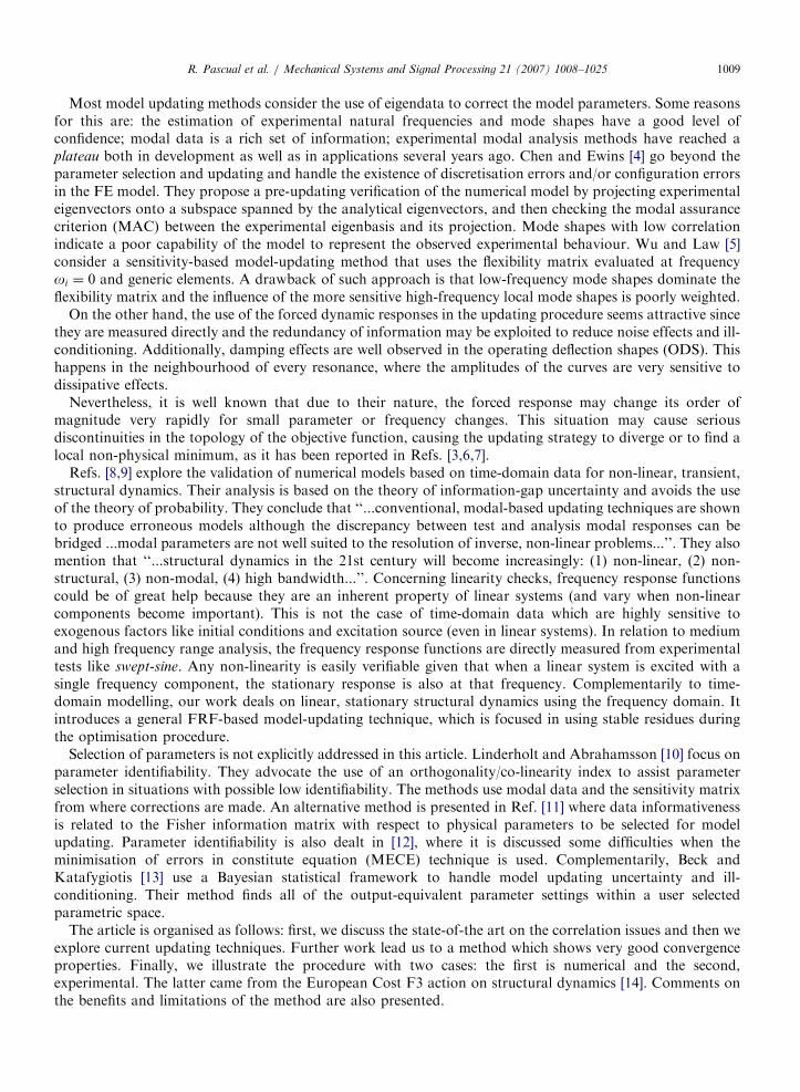
In a general situation, and referring to Fig. 1, it makes sense to compare the ODS that show the best mutualagreement, considering frequency shift. It should be pointed out that usually, as several parameters atelementary levels are perturbed, each one of these parameters will shift the eigenfrequencies in differentdirections so that an average frequency shift exists for each ODS. Correlation methods based on modal

Frequency

Am

plitu

de

FEExperimental

Fig. 1. Frequency response function of the reference and perturbed systems.


information (like the MAC [16] for instance) implicitly take the frequency shift into account, since they pairmode shapes at different frequencies: referring again to Fig. 1, the correlated mode pairs associated are not atthe same eigenfrequencies.

Nefske and Sung [17] propose to measure the correlation between two ODS at the same frequencies. In thiscase, a vector of correlation is obtained.

Based on the frequency shift mentioned above, we may measure the closeness between measured andsynthesised ODS by using the following correlation criterion:

FDACðoi;ojÞ ¼ �

ffiffiffiffiffiffiffiffiffiffiffiffiffiffiffiffiffiffiffiffiffiffiffiffiffiffiffiffiffiðhH

j hiÞHðhH

j hiÞ

ðhHj hjÞðh

Hi hiÞ

vuut , (4)

where oj corresponds to the frequency at which the numerical ODS hj is calculated, oi corresponds to onefrequency at which the experimental ODS hi was measured experimentally (the bar indicates that it ismeasured), and � indicates the relative phase of the ODS.

The so-called FDAC can be regarded as equivalent to the MAC in the frequency domain. It follows fromEq. (4) that FDAC values are limited to the interval ½�1; 1�. A value of 1 means perfect correlation, 0 nocorrelation at all, and �1 perfect correlation but a relative phase of 180�.

From FDAC, it is possible to define the frequency shift residue:

DoðojÞ ¼ o ji � oj, (5)

to measure the distance between the model and the test structure. oj represents the selected experimentalfrequency, and oj

i is the frequency at which FDACðoi;ojÞ reaches its maximum for oj 2 ½0;1Þ. Sampaio et al.[21] show the direct use of FDAC as a tool for damage detection.

A complementary measure of correlation is given by the frequency response scale factor (FRSF) defined asthe ratio of amplitudes:

FRSFðoi;ojÞ ¼

ffiffiffiffiffiffiffiffiffiffihH

j hj

hH

i hi

vuut . (6)

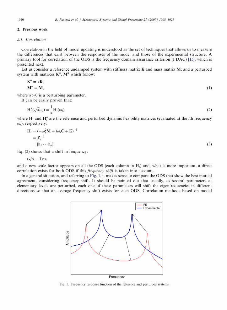
The evaluation of Eq. (4) for a given set of analytical frequencies and measured frequencies results in theFDAC matrix. A perfectly updated model will have only positive unitary values on the axis oi ¼ oj. Thespecial case considered in Eq. (1) appears clearly in the FDAC matrix as shown in Fig. 2. The stiffness factor

may be estimated easily from the slope of the line (oji ;oj).

Several other works deal with correlation issues using forced responses: Fotsch and Ewins [18] introduce atechnique where the criterion mixes operating deflection shapes and mode shapes to obtain directly the so-called correlated mode pairs between the model responses and the experimental data. Goge and Link [19] use aversion of FDAC at resonances that uses only the imaginary part of the ODS; in this way an increasedsensitivity to damping is obtained.

2.2. Model updating

It is well known that dynamic flexibility is a function of frequency which readily changes in amplitude.Therefore, a residue based on the difference between experimental and numerical ODS may be unstable,leading to numerical difficulties [7,20]. Refs. [22–24] avoid the problem by considering a residue using a log-least squares residue between test and model frequency response functions. Cha and Tuck-Lee [25] consider aformulation that enforces the connectivity patterns of the initial numerical model in a two step procedure: firstit adjusts the mass matrix, then the stiffness matrix. Other methods use the forced responses directly,exploiting the sensitivity with respect to the model parameters [20,26].

Let us assume the existence of the system matrices Kn; Cn and Mn with the same properties as thecorresponding analytical matrices. The dynamic equilibrium equation in the frequency domain is written as

ð�o2i M

n þ joiCnþ KnÞ hni ¼ f (7)

ARTICLE IN PRESS

600

500

400

300

200

100

00 100 200 300 400 500

FE frequency (Hz)

1

Exp

erim

enta

l fre

quen

cy (

Hz)

√√21

0.8

0.6

0.4

0.2

− 0.2

− 0.4

− 0.6

− 0.8

− 1

0

Fig. 2. FDAC for a ¼ 2 in Eqs. (1) and (4).

R. Pascual et al. / Mechanical Systems and Signal Processing 21 (2007) 1008–10251012

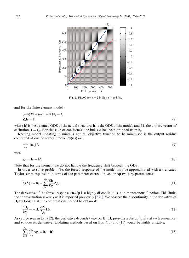
and for the finite element model:

ð�o2i Mþ joiCþ KÞ hi ¼ f,

Zihi ¼ f, ð8Þ

where hni is the assumed ODS of the actual structure; hi is the ODS of the model, and f is the unitary vector ofexcitation, f ¼ ek. For the sake of conciseness the index k has been dropped from hi.

Keeping model updating in mind, a natural objective function to be minimised is the output residuecomputed at one or several frequency(ies) oi:

minDpkedik2, (9)

with

edi¼ hi � hni . (10)

Note that for the moment we do not handle the frequency shift between the ODS.In order to solve problem (9), the forced response of the model may be approximated with a truncated

Taylor series expansion in terms of the parameter correction vector Dp (with np parameters):

hiðDpÞ ¼ hi þXnp

j¼1

qhi

qpj

Dpj . (11)

The derivative of the forced response qhi=qp is a highly discontinuous, non-monotonous function. This limitsthe approximation severely as it is reported previously [7,20]. We observe the discontinuity in the derivative ofHi by looking at the computations needed to obtain it:

qHi

qpj

¼ �Hi

qZi

qpj

Hi. (12)

As can be seen in Eq. (12), the derivative depends twice on Hi. Hi presents a discontinuity at each resonance,and so does its derivative. Updating methods based on Eqs. (10) and (11) would be highly unstable:

Xnp

j¼1

qhi

qpj

Dpj ¼ hi � hni . (13)


An alternative objective function that avoids the computation of Eq. (12), may be based on the minimisationof the input errors (or force errors) in the equation of motion, that is

minpkef ik2, (14)

with

ef i¼ Ziedi

¼ ek � Zihn

i . (15)

Similarly, the Taylor series expansion of Zi is used to solve problem (14):

ZiðpÞ ¼ Zi þXnp

j¼1

qZi

qpj

Dpj. (16)

This leads to the following updating equation:

Xnp

j¼1

qZi

qpj

Dpj

!hni � ek � Zih

n

i . (17)

An approximative equality has been written because the design parameters vector Dp may be an incompletelist (and also biased) of the true parameters corrections Dpn. Note that the measured hi always include somenoise n:

hi ¼ hni þ n (18)

that will inevitably perturb the updating equation, so that it is more correct to write:

Xnp

j¼1

qZi

qpj

Dpj

!hi � ek � Zihi. (19)

The noise term n appears on both sides of the equation multiplied by qZi=qp and Zi, respectively. This couplesthe noise in the updating equation and may induce biased and unstable results. To overcome the situation, aconvenient weighting matrix may be employed. If Eq. (19) is pre-multiplied by Hi, it becomes:

Hi

Xnp

j¼1

qZi

qpj

Dpj

!hi � hi � hi, (20)

which can be expressed as

ADp ¼ b, (21)

with

A ¼ Hi

qZi

qp1

hi; . . . ;qZi

qpnp

hi

" #,

b ¼ hi � hi.

Note that the right-hand side in Eq. (20) is the output residue that also appears in Eq. (13). The improvementis that the use of qhi=qp is avoided. Zi is a linear or quasi-linear explicit function of the parameters [20] so itsderivative qZi=qp shows a smooth behaviour; and its computation is straightforward. The introduction of Hi

reduces the effects of the noise term and improves the conditioning of the formulation [27]. Eq. (20) may beevaluated for a set of frequencies, in order to obtain the corrections Dp. These will define a new model, whichwill also be updated until the residue hi � hi stabilises at a minimum. Also note that each column in the matrixof coefficients A corresponds to the shape adopted by the structure according to the model for the externalforce configuration:

qZi

qpk

hi. (22)


The force (22) only operates in the degrees of freedom associated to the substructure k. If the substructuresbeing updated are close in space, their effects on the global dynamic behaviour will be similar. This maygenerate a set of columns almost linearly dependent in the left-hand side of Eq. (20), and the problem offinding the right Dp becomes ill-conditioned. To alleviate the problem, parameters should actuate on largersubstructures or macro-elements instead of single finite elements.

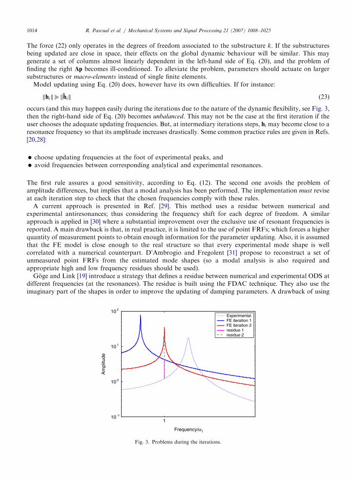
Model updating using Eq. (20) does, however have its own difficulties. If for instance:

khikbkhik (23)

occurs (and this may happen easily during the iterations due to the nature of the dynamic flexibility, see Fig. 3,then the right-hand side of Eq. (20) becomes unbalanced. This may not be the case at the first iteration if theuser chooses the adequate updating frequencies. But, at intermediary iterations steps, hi may become close to aresonance frequency so that its amplitude increases drastically. Some common practice rules are given in Refs.[20,28]:

�
choose updating frequencies at the foot of experimental peaks, and � avoid frequencies between corresponding analytical and experimental resonances.
The first rule assures a good sensitivity, according to Eq. (12). The second one avoids the problem ofamplitude differences, but implies that a modal analysis has been performed. The implementation must reviseat each iteration step to check that the chosen frequencies comply with these rules.

A current approach is presented in Ref. [29]. This method uses a residue between numerical andexperimental antiresonances; thus considering the frequency shift for each degree of freedom. A similarapproach is applied in [30] where a substantial improvement over the exclusive use of resonant frequencies isreported. A main drawback is that, in real practice, it is limited to the use of point FRFs; which forces a higherquantity of measurement points to obtain enough information for the parameter updating. Also, it is assumedthat the FE model is close enough to the real structure so that every experimental mode shape is wellcorrelated with a numerical counterpart. D’Ambrogio and Fregolent [31] propose to reconstruct a set ofunmeasured point FRFs from the estimated mode shapes (so a modal analysis is also required andappropriate high and low frequency residues should be used).

Goge and Link [19] introduce a strategy that defines a residue between numerical and experimental ODS atdifferent frequencies (at the resonances). The residue is built using the FDAC technique. They also use theimaginary part of the shapes in order to improve the updating of damping parameters. A drawback of using

110 -1

10 0

10 1

10 2

Frequency/ω i

Am

plitu

de

ExperimentalFE iteration 1FE iteration 2residue 1residue 2

Fig. 3. Problems during the iterations.


this approach is that it also needs a good starting FE model in order to correctly pair the ODS at theresonances.

3. Improved model updating

Taking into account the considerations described in Section 2.1, instead of comparing measured andanalytical operating shapes at the same frequency oi, the idea developed here is to define a more balancedresidue. For this purpose, let us use the following residue:

minpke0dik2, (24)

with

e0di¼ hj � hni , (25)

where two different frequencies are considered: oi for the experimental ODS and oj for the numerical ODS.It is easy to show that

Zn

i � Zj ¼ DZn

i þ jðoi � ojÞC� ðo2i � o2

j ÞM. (26)

This allows us to express a new force residue as

e0f i¼ Zie

0di

¼ � DZn

i hn

i þ jðoi � ojÞChn

i � ðo2i � o2

j ÞMhni

taking into account noise effects:

e0f i� �DZn

i hi þ jðoi � ojÞ Chi � ðo2i � o2

j Þ Mhi

and to alleviate the noise coupling, Hj is used:

Hje0f i� �HjDZ

n

i hi þ jðoi � ojÞHjChi � ðo2i � o2

j ÞHjMhi,

or

hj � hi � HjDZn

i hi þ jðoi � ojÞHjChi � ðo2i � o2

j ÞHjMhi.

Reordering

HjDZn

i hi � ðhj � hiÞ � jðoi � ojÞHjChi þ ðo2i � o2

j ÞHjMhi

and substituting the approximation to the exact DZn

i :

Hj

Xnp

j¼1

qZi

qpj

Dpj

!hi � ðhj � hiÞ � jðoi � ojÞHjChi þ ðo2

i � o2j ÞHjMhi. (27)

The right-hand side of Eq. (27) is composed of a residue representing the difference in the operating shapesplus the terms penalising their difference in frequency. Note that if oi ¼ oj, Eq. (27) is identical to Eq. (20).

3.1. Model reduction

The problem of model matching is addressed here by using dynamic reduction of the model matrices at eachfrequency. The reduced matrices are obtained through:

~Mi ¼ TTi MTi, (28)

~Zi ¼ TTi ZiTi, (29)

where Ti corresponds to the operator of the dynamic expansion technique [32] (superscript � is used for allvariables related to the reduced model).


An advantage of this reduction approach is that it avoids approximations in the dynamic response of thereduced system:

~Hi ¼ HmmðiÞ, (30)

where mm represents the measured partition of degrees of freedom.In order to use Eq. (27) we need to find also q ~Zi=qpk. The dynamic flexibility matrix of the reduced model is

by definition:

~Hi ¼ ~Z�1

i (31)

and the sensitivities of the reduced dynamic stiffness with respect to the design parameters are obtainedthrough the identity relationships:

qHi

qpk

¼ �Hi

qZi

qpk

Hi ¼dHk

mmðiÞ dHkmoðiÞ

dHkomðiÞ dHk

ooðiÞ

24

35, (32)

qZi

qpk

¼ �Zi

qHi

qpk

Zi, (33)

where o represents the unmeasured partition of degrees of freedom.Recalling that

dHkmmðiÞ ¼

q ~Hi

qpk

(34)

leads to

q ~Zi

qpk

¼ ~Zi dHkmmðiÞ

~Zi, (35)

thus, problem (20) is implemented using the following equation:

~Hi

Xnp

j¼1

q ~Zi

qpj

Dpj

!hi � ~hi � hi. (36)

The improved method (27) is implemented using:

~Hj

Xnp

j¼1

q ~Zi

qpj

Dpj

!hi � ð~hj � hiÞ � jðoi � ojÞ ~Hj

~Chi þ ðo2i � o2

j Þ~Hj~Mhi. (37)

A drawback of any method based on reduction (28) is that it is valid only at one frequency oj; and severalfrequencies may be used to handle noise.

4. Numerical example

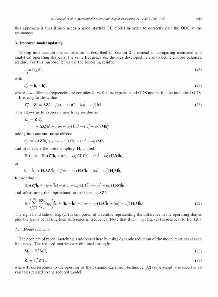
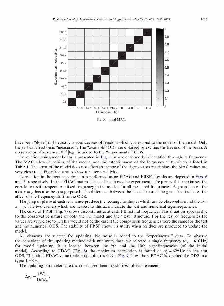
This example considers a cantilever beam extensively used in the bibliography. The model is composed of 15Euler–Bernoulli beam elements (Fig. 4). The ‘‘experimental’’ structure differs from the initial FE model by thebending stiffness of the element 8 which has been doubled in the ‘‘experimental’’ structure. Measurements

l = 1.80 m, A = 10-4 m2, E = 2.1011 Pa,I = 8.33 10-10 m4, ρ = 7800 kg/m3.

Fig. 4. The clamped beam.

ARTICLE IN PRESS

2.5 15.8 44.2 86.8 143.5 214.5 300 400 515 645.4

2.5

16.3

44.3

89.9

143.8

222.2

301.4

414.0

518.9

666.8

FE modes (Hz)

Exp

erim

enta

l mod

es (

Hz)

0

0.1

0.2

0.3

0.4

0.5

0.6

0.7

0.8

0.9

1

Fig. 5. Initial MAC.

R. Pascual et al. / Mechanical Systems and Signal Processing 21 (2007) 1008–1025 1017

have been ‘‘done’’ in 15 equally spaced degrees of freedom which correspond to the nodes of the model. Onlythe vertical direction is ‘‘measured’’. The ‘‘available’’ ODS are obtained by exciting the free end of the beam. Anoise vector of variance 10�2 hðiÞ

�� is added to the ‘‘experimental’’ ODS.Correlation using modal data is presented in Fig. 5, where each mode is identified through its frequency.

The MAC allows a pairing of the modes, and the establishment of the frequency shift, which is listed inTable 1. The error of the model does not affect the shape of the eigenvectors much since the MAC values arevery close to 1. Eigenfrequencies show a better sensitivity.

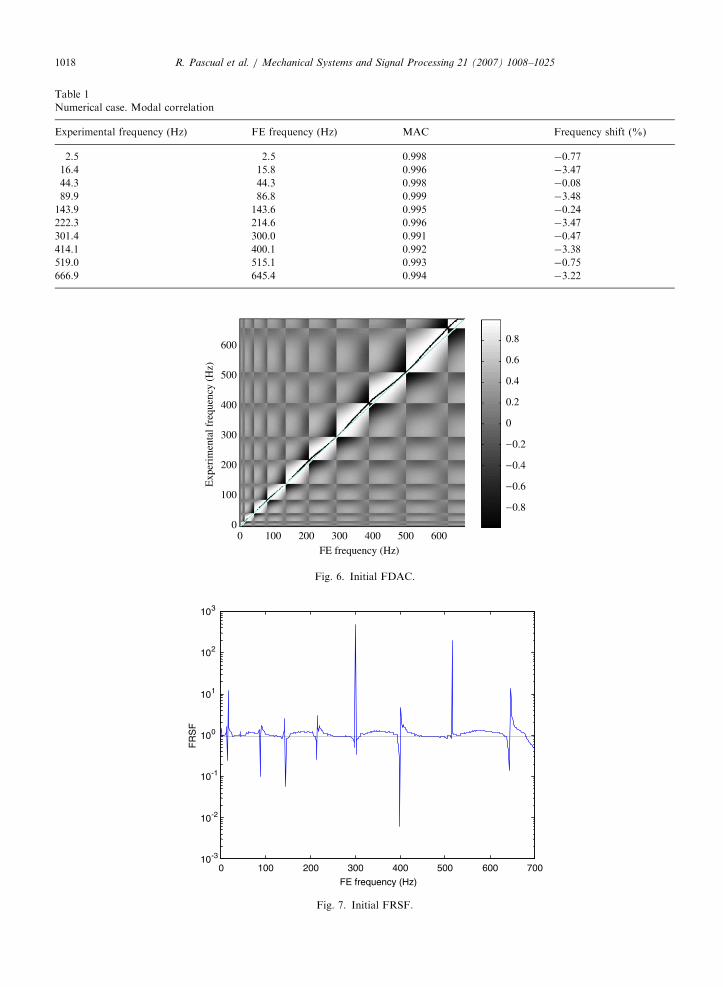
Correlation in the frequency domain is performed using FDAC and FRSF. Results are depicted in Figs. 6and 7, respectively. In the FDAC matrix a black line shows the experimental frequency that maximises thecorrelation with respect to a fixed frequency in the model, for all measured frequencies. A green line on theaxis x ¼ y has also been superposed. The difference between the black line and the green line indicates theeffect of the frequency shift in the ODS.

The jump of phase at each resonance produce the rectangular shapes which can be observed around the axisx ¼ y. The two corners which are nearest to this axis indicate the test and numerical eigenfrequencies.

The curve of FRSF (Fig. 7) shows discontinuities at each FE natural frequency. This situation appears dueto the conservative nature of both the FE model and the ‘‘test’’ structure. For the rest of frequencies thevalues are very close to 1. This would not be the case if the comparison frequencies were the same for the testand the numerical ODS. The stability of FRSF shows its utility when residues are produced to update themodel.

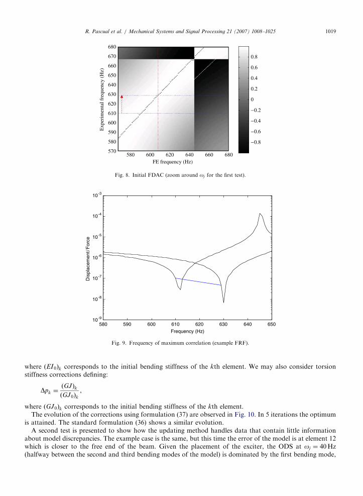
All elements are selected for updating. No noise is added to the ‘‘experimental’’ data. To observethe behaviour of the updating method with minimum data, we selected a single frequency ðoj ¼ 610HzÞfor model updating. It is located between the 9th and the 10th eigenfrequencies (of the initialmodel). According to FDAC (Fig. 8) the maximum correlation is found at oi

j ¼ 629Hz in the testODS. The initial FDAC value (before updating) is 0.994. Fig. 9 shows how FDAC has paired the ODS in atypical FRF.

The updating parameters are the normalised bending stiffness of each element:

Dpk ¼ðEIÞkðEI0Þk

,

ARTICLE IN PRESS

Table 1

Numerical case. Modal correlation

Experimental frequency (Hz) FE frequency (Hz) MAC Frequency shift (%)

2.5 2.5 0.998 �0.77

16.4 15.8 0.996 �3.47

44.3 44.3 0.998 �0.08

89.9 86.8 0.999 �3.48

143.9 143.6 0.995 �0.24

222.3 214.6 0.996 �3.47

301.4 300.0 0.991 �0.47

414.1 400.1 0.992 �3.38

519.0 515.1 0.993 �0.75

666.9 645.4 0.994 �3.22

600

500

400

300

200

100

00 100 200 300 400 500 600

FE frequency (Hz)

Exp

erim

enta

l fre

quen

cy (

Hz)

0.8

0.6

0.4

0.2

− 0.2

− 0.4

− 0.6

− 0.8

0

Fig. 6. Initial FDAC.

0 100 200 300 400 500 600 70010-3

10-2

10-1

100

101

102

103

FE frequency (Hz)

FR

SF

Fig. 7. Initial FRSF.


ARTICLE IN PRESS

680

670

660

650

640

630

620

610

600

590

580

580 600 620 640 660 680570

FE frequency (Hz)

Exp

erim

enta

l fre

quen

cy (

Hz)

0.8

0.6

0.4

0.2

− 0.2

− 0.4

− 0.6

− 0.8

0

Fig. 8. Initial FDAC (zoom around oj for the first test).

580 590 600 610 620 630 640 65010-9

10-8

10-7

10-6

10-5

10-4

10-3

Frequency (Hz)

Dis

plac

emen

t/F

orce

Fig. 9. Frequency of maximum correlation (example FRF).


where ðEI0Þk corresponds to the initial bending stiffness of the kth element. We may also consider torsionstiffness corrections defining:

Dpk ¼ðGJÞkðGJ0Þk

,

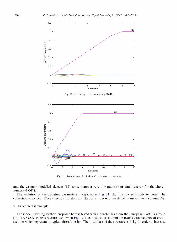
where ðGJ0Þk corresponds to the initial bending stiffness of the kth element.The evolution of the corrections using formulation (37) are observed in Fig. 10. In 5 iterations the optimum

is attained. The standard formulation (36) shows a similar evolution.A second test is presented to show how the updating method handles data that contain little information

about model discrepancies. The example case is the same, but this time the error of the model is at element 12which is closer to the free end of the beam. Given the placement of the exciter, the ODS at oj ¼ 40Hz(halfway between the second and third bending modes of the model) is dominated by the first bending mode,

ARTICLE IN PRESS

0 1 2 3 4 5 6 7-0.2

0

0.2

0.4

0.6

0.8

1

1.2

Iterations

Upd

atin

g pa

ram

eter

s

K8

Fig. 10. Updating corrections using 610Hz.

Iterations0 2 4 6 8 10 12 14 16

-0.2

0

0.2

0.4

0.6

0.8

1

1.2

Upd

atin

g pa

ram

eter

s

K1K2

K3K4 K5 K6 K7

K8K9 K10 K11

K12

K13 K14 K15

Fig. 11. Second case. Evolution of parameter corrections.


and the wrongly modelled element (12) concentrates a very low quantity of strain energy for the chosennumerical ODS.

The evolution of the updating parameters is depicted in Fig. 11, showing low sensitivity to noise. Thecorrection to element 12 is perfectly estimated, and the corrections of other elements amount to maximum 6%.

5. Experimental example

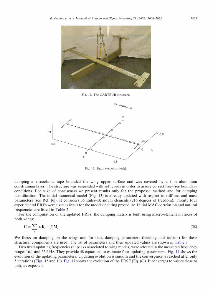
The model updating method proposed here is tested with a benchmark from the European Cost F3 Group[14]. The GARTEUR structure is shown in Fig. 12. It consists of six aluminium beams with rectangular cross-sections which represents a typical aircraft design. The total mass of the structure is 44 kg. In order to increase

ARTICLE IN PRESS

Fig. 12. The GARTEUR structure.

-0.8

0

-0.8

0

0.8

X

22

2120

23

19

36

1817

3532

31

30

16

34

29

33

14 15

28

131227

11

Y

1098

26

7654443

24

2111

25

Z

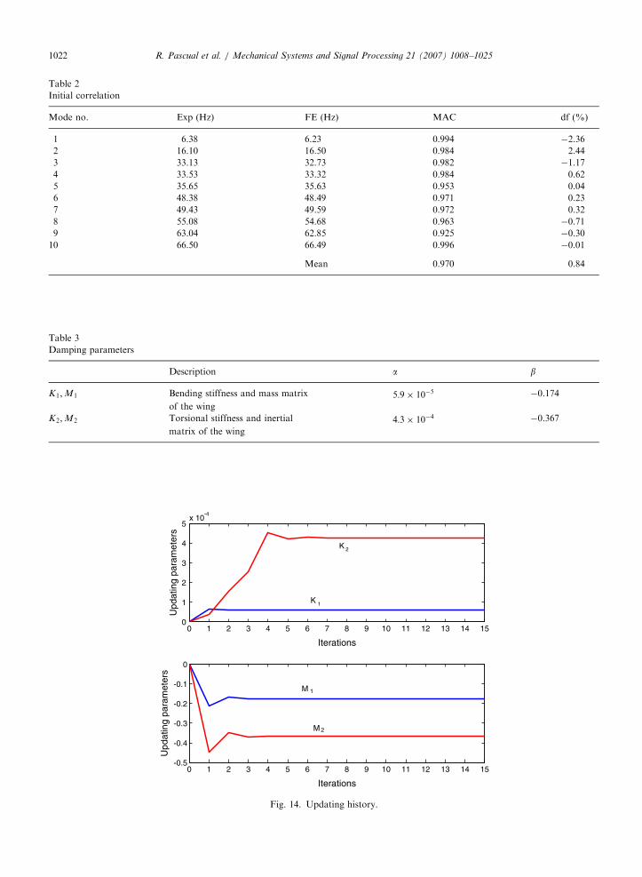
Fig. 13. Beam elements model.


damping a viscoelastic tape bounded the wing upper surface and was covered by a thin aluminiumconstraining layer. The structure was suspended with soft cords in order to assure correct free–free boundaryconditions. For sake of conciseness we present results only for the proposed method and for dampingidentification. The initial numerical model (Fig. 13) is already updated with respect to stiffness and massparameters (see Ref. [6]). It considers 35 Euler–Bernoulli elements (216 degrees of freedom). Twenty fourexperimental FRFs were used as input for the model updating procedure. Initial MAC correlation and naturalfrequencies are listed in Table 2.

For the computation of the updated FRFs, the damping matrix is built using macro-element matrices ofboth wings:

C ¼X

j

ajKj þ bjMj. (38)

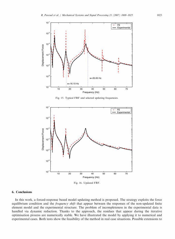
We focus on damping on the wings and for that, damping parameters (bending and torsion) for thesestructural components are used. The list of parameters and their updated values are shown in Table 3.

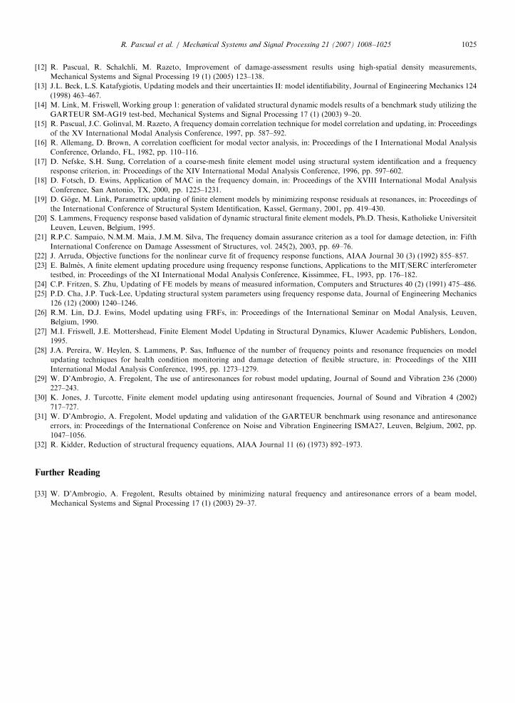
Two fixed updating frequencies (at peaks associated to wing modes) were selected in the measured frequencyrange: 16.1 and 35:6Hz. They provide 48 equations to estimate four updating parameters. Fig. 14 shows theevolution of the updating parameters. Updating evolution is smooth and the convergence is reached after only5 iterations (Figs. 15 and 16). Fig. 17 shows the evolution of the FRSF (Eq. (6)). It converges to values close tounit, as expected.

ARTICLE IN PRESS

Table 3

Damping parameters

Description a b

K1;M1 Bending stiffness and mass matrix 5:9 10�5 �0.174

of the wing

K2;M2 Torsional stiffness and inertial 4:3 10�4 �0.367

matrix of the wing

Table 2

Initial correlation

Mode no. Exp (Hz) FE (Hz) MAC df (%)

1 6.38 6.23 0.994 �2.36

2 16.10 16.50 0.984 2.44

3 33.13 32.73 0.982 �1.17

4 33.53 33.32 0.984 0.62

5 35.65 35.63 0.953 0.04

6 48.38 48.49 0.971 0.23

7 49.43 49.59 0.972 0.32

8 55.08 54.68 0.963 �0.71

9 63.04 62.85 0.925 �0.30

10 66.50 66.49 0.996 �0.01

Mean 0.970 0.84

0 1 2 3 4 5 6 7 8 9 10 11 12 13 14 150

1

2

3

4

5x 10

-4

Upd

atin

g pa

ram

eter

s

Iterations

0 1 2 3 4 5 6 7 8 9 10 11 12 13 14 15-0.5

-0.4

-0.3

-0.2

-0.1

0

Upd

atin

g pa

ram

eter

s

Iterations

M

M

K

K 2

1

2

1

Fig. 14. Updating history.


ARTICLE IN PRESS

10 20 30 40 50 60 7010-7

10-6

10-5

10-4

10-3

10-2

10-1

Frequency (Hz)

Dis

plac

emen

t/F

orce

FE Experimental

w=35.65 Hz

w=16.10 Hz

Fig. 15. Typical FRF and selected updating frequencies.

10 20 30 40 50 60 7010-7

10-6

10-5

10-4

10-3

10-2

10-1

Frequency (Hz)

Dis

plac

emen

t/F

orce

FE Experimental

Fig. 16. Updated FRF.


6. Conclusions

In this work, a forced-response based model updating method is proposed. The strategy exploits the forceequilibrium condition and the frequency shift that appear between the responses of the non-updated finiteelement model and the experimental structure. The problem of incompleteness in the experimental data ishandled via dynamic reduction. Thanks to the approach, the residues that appear during the iterativeoptimisation process are numerically stable. We have illustrated the model by applying it to numerical andexperimental cases. Both tests show the feasibility of the method in real case situations. Possible extensions to

ARTICLE IN PRESS

0 5 10 150

1

2

3

4

5

6

7

8

9

10

Iterations

FR

SF

ω=16.10 Hz ω=35.65 Hz

Fig. 17. FRSF non-shifted during iterations.


the methods include the use of alternative criteria to select the frequencies used to generate residues. Forexample, instead of using best correlation (FDAC) we may also use some minimum distance betweenexperimental and numerical ODS.

Acknowledgements

The authors wish to acknowledge the partial financial support of this study by the FOndo Nacional deDEsarrollo Cientıfico Y Tecnologico (FONDECYT) of the Chilean government (projects 1020810 and1030943).

References

[1] G.H. Kim, Y.S. Park, An improved updating parameter selection method and finite element model update using multiobjective

optimisation technique, Mechanical Systems and Signal Processing 18 (1) (2004) 59–78.

[2] R. Camillacci, S. Gabriele, Mechanical identification and model validation for shear-type frames, Mechanical Systems and Signal

Processing 19 (3) (2005) 597–614.

[3] W. Heylen, S. Lammens, P. Sas, Modal Analysis Theory and Testing, Katholieke Universiteit Leuven, Belgium, 1998.

[4] G. Chen, D.J. Ewins, FE model verification for structural dynamics with vector projection, Mechanical Systems and Signal

Processing 18 (4) (2004) 739–757.

[5] D. Wu, S.S. Law, Model error correction from truncated modal flexibility sensitivity and generic parameters: part I—simulation,

Mechanical Systems and Signal Processing 18 (6) (2004) 1381–1399.

[6] R. Pascual, M. Razeto, J. Golinval, R. Schalchli, A robust FRF-based technique for model updating, in: Proceedings of the

International Conference on Noise and Vibration Engineering ISMA27, Leuven, Belgium, 2002, pp. 1037–1045.

[7] S. Cogan, D. Lenoir, G. Lallement, J.N. Bricout, An improved frequency response residual for model correction, in: Proceedings of

the XIV International Modal Analysis Conference. Dearborn, MI, 1996, pp. 568–575.

[8] F.M. Hemez, S.W. Doebling, Review and assessment of model updating for non-linear, transient dynamics, Mechanical Systems and

Signal Processing 15 (1) (2001) 45–74.

[9] F.M. Hemez, Y. Ben-Haim, Info-gap robustness for the correlation of tests and simulations of a non-linear transient, Mechanical

Systems and Signal Processing 18 (6) (2004) 1443–1467.

[10] A. Linderholt, T. Abrahamsson, Parameter identifiability in finite element model error localisation, Mechanical Systems and Signal

Processing 17 (3) (2003) 579–588.

[11] A. Linderholt, T. Abrahamsson, Optimising the informativeness of test data used for computational model updating, Mechanical

Systems and Signal Processing 19 (4) (2005) 736–750.


[12] R. Pascual, R. Schalchli, M. Razeto, Improvement of damage-assessment results using high-spatial density measurements,


[13] J.L. Beck, L.S. Katafygiotis, Updating models and their uncertainties II: model identifiability, Journal of Engineering Mechanics 124

(1998) 463–467.

[14] M. Link, M. Friswell, Working group 1: generation of validated structural dynamic models results of a benchmark study utilizing the

GARTEUR SM-AG19 test-bed, Mechanical Systems and Signal Processing 17 (1) (2003) 9–20.

[15] R. Pascual, J.C. Golinval, M. Razeto, A frequency domain correlation technique for model correlation and updating, in: Proceedings

of the XV International Modal Analysis Conference, 1997, pp. 587–592.

[16] R. Allemang, D. Brown, A correlation coefficient for modal vector analysis, in: Proceedings of the I International Modal Analysis

Conference, Orlando, FL, 1982, pp. 110–116.

[17] D. Nefske, S.H. Sung, Correlation of a coarse-mesh finite element model using structural system identification and a frequency

response criterion, in: Proceedings of the XIV International Modal Analysis Conference, 1996, pp. 597–602.

[18] D. Fotsch, D. Ewins, Application of MAC in the frequency domain, in: Proceedings of the XVIII International Modal Analysis

Conference, San Antonio, TX, 2000, pp. 1225–1231.

[19] D. Goge, M. Link, Parametric updating of finite element models by minimizing response residuals at resonances, in: Proceedings of

the International Conference of Structural System Identification, Kassel, Germany, 2001, pp. 419–430.

[20] S. Lammens, Frequency response based validation of dynamic structural finite element models, Ph.D. Thesis, Katholieke Universiteit

Leuven, Leuven, Belgium, 1995.

[21] R.P.C. Sampaio, N.M.M. Maia, J.M.M. Silva, The frequency domain assurance criterion as a tool for damage detection, in: Fifth

International Conference on Damage Assessment of Structures, vol. 245(2), 2003, pp. 69–76.

[22] J. Arruda, Objective functions for the nonlinear curve fit of frequency response functions, AIAA Journal 30 (3) (1992) 855–857.

[23] E. Balmes, A finite element updating procedure using frequency response functions, Applications to the MIT/SERC interferometer

testbed, in: Proceedings of the XI International Modal Analysis Conference, Kissimmee, FL, 1993, pp. 176–182.

[24] C.P. Fritzen, S. Zhu, Updating of FE models by means of measured information, Computers and Structures 40 (2) (1991) 475–486.

[25] P.D. Cha, J.P. Tuck-Lee, Updating structural system parameters using frequency response data, Journal of Engineering Mechanics

126 (12) (2000) 1240–1246.

[26] R.M. Lin, D.J. Ewins, Model updating using FRFs, in: Proceedings of the International Seminar on Modal Analysis, Leuven,

Belgium, 1990.

[27] M.I. Friswell, J.E. Mottershead, Finite Element Model Updating in Structural Dynamics, Kluwer Academic Publishers, London,

1995.

[28] J.A. Pereira, W. Heylen, S. Lammens, P. Sas, Influence of the number of frequency points and resonance frequencies on model

updating techniques for health condition monitoring and damage detection of flexible structure, in: Proceedings of the XIII

International Modal Analysis Conference, 1995, pp. 1273–1279.

[29] W. D’Ambrogio, A. Fregolent, The use of antiresonances for robust model updating, Journal of Sound and Vibration 236 (2000)

227–243.

[30] K. Jones, J. Turcotte, Finite element model updating using antiresonant frequencies, Journal of Sound and Vibration 4 (2002)

717–727.

[31] W. D’Ambrogio, A. Fregolent, Model updating and validation of the GARTEUR benchmark using resonance and antiresonance

errors, in: Proceedings of the International Conference on Noise and Vibration Engineering ISMA27, Leuven, Belgium, 2002, pp.

1047–1056.

[32] R. Kidder, Reduction of structural frequency equations, AIAA Journal 11 (6) (1973) 892–1973.

Further Reading

[33] W. D’Ambrogio, A. Fregolent, Results obtained by minimizing natural frequency and antiresonance errors of a beam model,


Robust parameter identification using forced responses

Documents