Robust ML Training with Conditional Gradients Sebastian Pokutta Technische Universität Berlin and Zuse Institute Berlin [email protected] @spokutta CO@Work 2020 Summer School September, 2020 Berlin Mathematics Research Center MATH

Welcome message from author
This document is posted to help you gain knowledge. Please leave a comment to let me know what you think about it! Share it to your friends and learn new things together.
Transcript
Robust ML Training with Conditional Gradients
Sebastian Pokutta
Technische Universität Berlinand
Zuse Institute Berlin
[email protected]@spokutta
CO@Work 2020 Summer SchoolSeptember, 2020
Berlin Mathematics Research Center
MATHSTYLEGUIDE

Opportunities in BerlinShameless plug
Postdoc and PhD positions in optimization/ML.
At Zuse Institute Berlin and TU Berlin.
Sebastian Pokutta · Training with Conditional Gradients 1 / 14

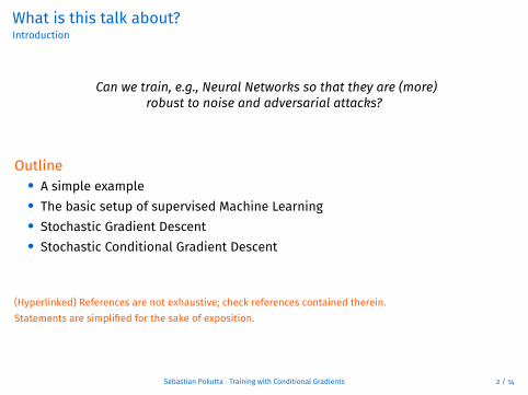
What is this talk about?Introduction
Can we train, e.g., Neural Networks so that they are (more)robust to noise and adversarial attacks?
Outline• A simple example• The basic setup of supervised Machine Learning• Stochastic Gradient Descent• Stochastic Conditional Gradient Descent
(Hyperlinked) References are not exhaustive; check references contained therein.Statements are simplified for the sake of exposition.
Sebastian Pokutta · Training with Conditional Gradients 2 / 14

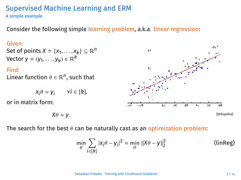
Supervised Machine Learning and ERMA simple example
Consider the following simple learning problem, a.k.a. linear regression:
Given:Set of points X � {x1, . . . ,xk} ⊆ Rn
Vector y � (y1, . . . ,yk) ∈ Rk
Find:Linear function θ ∈ Rn, such that
xiθ ≈ yi ∀i ∈ [k],
or in matrix form:
Xθ ≈ y. [Wikipedia]
The search for the best θ can be naturally cast as an optimization problem:
minθ
∑i∈[k]|xiθ − yi |
2 = minθ‖Xθ − y‖22 (linReg)
Sebastian Pokutta · Training with Conditional Gradients 3 / 14

Supervised Machine Learning and ERMEmpirical Risk Minimization
More generally, interested in the Empirical Risk Minimization problem:
minθL(θ) � min
θ
1|D|
∑(x,y)∈D
`(f (x, θ),y). (ERM)
The ERM approximates the General Risk Minimization problem:
minθL̂(θ) � min
θE(x,y)∈D̂ `(f (x, θ),y). (GRM)
Note: If D is chosen large enough, under relatively mild assumptions, a solution to(ERM) is a good approximation to a solution to (GRM):
L̂(θ) ≤ L(θ) +
√log|Θ| + log 1
δ
|D|,
with probability 1 − δ. This bound is typically very loose.[ e.g., Suriya Gunasekar’ lecture notes] [The Elements of Statistical Learning, Hastie et al]
Sebastian Pokutta · Training with Conditional Gradients 4 / 14

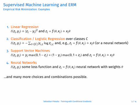
Supervised Machine Learning and ERMEmpirical Risk Minimization: Examples
1. Linear Regression`(zi,yi) � |zi − yi |2 and zi = f (θ,xi) � xiθ
2. Classification / Logistic Regression over classes C`(zi,yi) � −
∑c∈[C] yi,c log zi,c and, e.g., zi = f (θ,xi) � xiθ (or a neural network)
3. Support Vector Machines`(zi,yi) � yimax(0,1 − zi) + (1 − yi)max(0,1 + zi) and zi = f (θ,xi) � xiθ
4. Neural Networks`(zi,yi) some loss function and zi = f (θ,xi) neural network with weights θ
...and many more choices and combinations possible.
Sebastian Pokutta · Training with Conditional Gradients 5 / 14
Optimizing the ERM ProblemStochastic Gradient Descent
How to solve Problem (ERM)?
Simple idea: Gradient Descent [see blog for background on conv opt]
θt+1 ← θt − η∇L(θt) (GD)
Unfortunately, this might be too expensive if (ERM) has a lot of summands.
However, reexamine:
∇L(θ) = ∇ 1|D|
∑(x,y)∈D
`(f (x, θ),y) = 1|D|
∑(x,y)∈D
∇`(f (x, θ),y), (ERMgrad)
Thus if we sample (x,y) ∈ D uniformly at random, then
∇L(θ) = E(x,y)∈D∇`(f (x, θ),y) (gradEst)
Sebastian Pokutta · Training with Conditional Gradients 6 / 14

Optimizing the ERM ProblemStochastic Gradient Descent
This leads to Stochastic Gradient Descent
θt+1 ← θt − η∇`(f (x, θt),y) with (x,y) ∼ D, (SGD)
one of the most-used algorithm for ML training (together with its many variants).
Typical variants include• Batch versions. Rather than just taking one stochastic gradient, sample andaverage a mini batch. This also reduces variance of the gradient estimator.• Learning rate schedules. To ensure convergence the learning rate η is dynamicallymanaged.• Adaptive Variants and Momentum. RMSProp, Adagrad, Adadelta, Adam, ...• Variance Reduction. Compute exact gradient once in a while as reference point,e.g., SVRG.
[for an overview of variants: blog of Sebastian Ruder]
Sebastian Pokutta · Training with Conditional Gradients 7 / 14

Optimizing the ERM ProblemStochastic Gradient Descent
This leads to Stochastic Gradient Descent
θt+1 ← θt − η∇`(f (x, θt),y) with (x,y) ∼ D, (SGD)
one of the most-used algorithm for ML training (together with its many variants).
Typical variants include• Batch versions. Rather than just taking one stochastic gradient, sample andaverage a mini batch. This also reduces variance of the gradient estimator.
• Learning rate schedules. To ensure convergence the learning rate η is dynamicallymanaged.• Adaptive Variants and Momentum. RMSProp, Adagrad, Adadelta, Adam, ...• Variance Reduction. Compute exact gradient once in a while as reference point,e.g., SVRG.
[for an overview of variants: blog of Sebastian Ruder]
Sebastian Pokutta · Training with Conditional Gradients 7 / 14

Optimizing the ERM ProblemStochastic Gradient Descent
This leads to Stochastic Gradient Descent
θt+1 ← θt − η∇`(f (x, θt),y) with (x,y) ∼ D, (SGD)
one of the most-used algorithm for ML training (together with its many variants).
Typical variants include• Batch versions. Rather than just taking one stochastic gradient, sample andaverage a mini batch. This also reduces variance of the gradient estimator.• Learning rate schedules. To ensure convergence the learning rate η is dynamicallymanaged.
• Adaptive Variants and Momentum. RMSProp, Adagrad, Adadelta, Adam, ...• Variance Reduction. Compute exact gradient once in a while as reference point,e.g., SVRG.
[for an overview of variants: blog of Sebastian Ruder]
Sebastian Pokutta · Training with Conditional Gradients 7 / 14

Optimizing the ERM ProblemStochastic Gradient Descent
This leads to Stochastic Gradient Descent
θt+1 ← θt − η∇`(f (x, θt),y) with (x,y) ∼ D, (SGD)
one of the most-used algorithm for ML training (together with its many variants).
Typical variants include• Batch versions. Rather than just taking one stochastic gradient, sample andaverage a mini batch. This also reduces variance of the gradient estimator.• Learning rate schedules. To ensure convergence the learning rate η is dynamicallymanaged.• Adaptive Variants and Momentum. RMSProp, Adagrad, Adadelta, Adam, ...
• Variance Reduction. Compute exact gradient once in a while as reference point,e.g., SVRG.
[for an overview of variants: blog of Sebastian Ruder]
Sebastian Pokutta · Training with Conditional Gradients 7 / 14

Optimizing the ERM ProblemStochastic Gradient Descent
This leads to Stochastic Gradient Descent
θt+1 ← θt − η∇`(f (x, θt),y) with (x,y) ∼ D, (SGD)
one of the most-used algorithm for ML training (together with its many variants).
Typical variants include• Batch versions. Rather than just taking one stochastic gradient, sample andaverage a mini batch. This also reduces variance of the gradient estimator.• Learning rate schedules. To ensure convergence the learning rate η is dynamicallymanaged.• Adaptive Variants and Momentum. RMSProp, Adagrad, Adadelta, Adam, ...• Variance Reduction. Compute exact gradient once in a while as reference point,e.g., SVRG.
[for an overview of variants: blog of Sebastian Ruder]
Sebastian Pokutta · Training with Conditional Gradients 7 / 14

A comparison between different variantsStochastic Gradient Descent
[Graphics from blog of Sebastian Ruder; see also for animations]
Sebastian Pokutta · Training with Conditional Gradients 8 / 14

(More) robust ERM trainingStochastic Conditional Gradients
Recall Problem (ERM):
minθ
1|D|
∑(x,y)∈D
`(f (x, θ),y).
In the standard formulation θ is unbounded and can get quite large.
Problem. Large θ for, e.g., Neural Networks lead to large Lipschitz constants. Trainednetwork becomes sensitive to input noise and perturbations. [Tsuzuku, Sato, Sugiyama, 2018]
test set accuracy
0 20 40 60 80 100
epoch0.2
0.3
0.4
0.5
0.6
0.7
0.8
test set accuracy with noise (σ = 0.3)
0 20 40 60 80 100
epoch0.2
0.3
0.4
0.5
0.6
0.7
0.8
test set accuracy with noise (σ = 0.6)
0 20 40 60 80 100
epoch0.2
0.3
0.4
0.5
0.6
0.7
0.8
Performance for Neural Network trained on MNIST.
Sebastian Pokutta · Training with Conditional Gradients 9 / 14

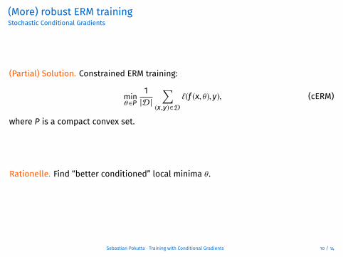
(More) robust ERM trainingStochastic Conditional Gradients
(Partial) Solution. Constrained ERM training:
minθ∈P
1|D|
∑(x,y)∈D
`(f (x, θ),y), (cERM)
where P is a compact convex set.
Rationelle. Find “better conditioned” local minima θ.
Sebastian Pokutta · Training with Conditional Gradients 10 / 14
(More) robust ERM trainingStochastic Conditional Gradients
(Partial) Solution. Constrained ERM training:
minθ∈P
1|D|
∑(x,y)∈D
`(f (x, θ),y), (cERM)
where P is a compact convex set.
Rationelle. Find “better conditioned” local minima θ.
Sebastian Pokutta · Training with Conditional Gradients 10 / 14
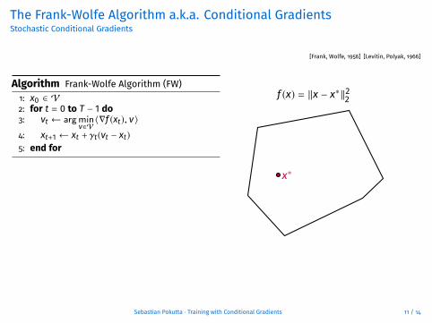
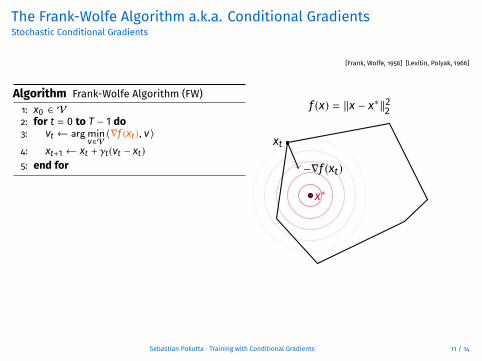
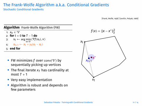
The Frank-Wolfe Algorithm a.k.a. Conditional GradientsStochastic Conditional Gradients
[Frank, Wolfe, 1956] [Levitin, Polyak, 1966]
Algorithm Frank-Wolfe Algorithm (FW)1: x0 ∈ V2: for t = 0 to T − 1 do3: vt ← argmin
v∈V〈∇f (xt), v〉
4: xt+1 ← xt + γt(vt − xt)5: end for
• FW minimizes f over conv(V) bysequentially picking up vertices• The final iterate xT has cardinality atmost T + 1• Very easy implementation• Algorithm is robust and depends onfew parameters
f (x) = ‖x − x∗‖22
xt
vt
−∇f (xt)
x∗
xt+1
Sebastian Pokutta · Training with Conditional Gradients 11 / 14

The Frank-Wolfe Algorithm a.k.a. Conditional GradientsStochastic Conditional Gradients
[Frank, Wolfe, 1956] [Levitin, Polyak, 1966]
Algorithm Frank-Wolfe Algorithm (FW)1: x0 ∈ V2: for t = 0 to T − 1 do3: vt ← argmin
v∈V〈∇f (xt), v〉
4: xt+1 ← xt + γt(vt − xt)5: end for
• FW minimizes f over conv(V) bysequentially picking up vertices• The final iterate xT has cardinality atmost T + 1• Very easy implementation• Algorithm is robust and depends onfew parameters
f (x) = ‖x − x∗‖22
xt
vt
−∇f (xt)
x∗xt+1
Sebastian Pokutta · Training with Conditional Gradients 11 / 14

The Frank-Wolfe Algorithm a.k.a. Conditional GradientsStochastic Conditional Gradients
[Frank, Wolfe, 1956] [Levitin, Polyak, 1966]
Algorithm Frank-Wolfe Algorithm (FW)1: x0 ∈ V2: for t = 0 to T − 1 do3: vt ← argmin
v∈V〈∇f (xt), v〉
4: xt+1 ← xt + γt(vt − xt)5: end for
• FW minimizes f over conv(V) bysequentially picking up vertices
• The final iterate xT has cardinality atmost T + 1• Very easy implementation• Algorithm is robust and depends onfew parameters
f (x) = ‖x − x∗‖22
xt
vt
−∇f (xt)
x∗xt+1
Sebastian Pokutta · Training with Conditional Gradients 11 / 14

The Frank-Wolfe Algorithm a.k.a. Conditional GradientsStochastic Conditional Gradients
[Frank, Wolfe, 1956] [Levitin, Polyak, 1966]
Algorithm Frank-Wolfe Algorithm (FW)1: x0 ∈ V2: for t = 0 to T − 1 do3: vt ← argmin
v∈V〈∇f (xt), v〉
4: xt+1 ← xt + γt(vt − xt)5: end for
• FW minimizes f over conv(V) bysequentially picking up vertices• The final iterate xT has cardinality atmost T + 1
• Very easy implementation• Algorithm is robust and depends onfew parameters
f (x) = ‖x − x∗‖22
xt
vt
−∇f (xt)
x∗xt+1
Sebastian Pokutta · Training with Conditional Gradients 11 / 14

The Frank-Wolfe Algorithm a.k.a. Conditional GradientsStochastic Conditional Gradients
[Frank, Wolfe, 1956] [Levitin, Polyak, 1966]
Algorithm Frank-Wolfe Algorithm (FW)1: x0 ∈ V2: for t = 0 to T − 1 do3: vt ← argmin
v∈V〈∇f (xt), v〉
4: xt+1 ← xt + γt(vt − xt)5: end for
• FW minimizes f over conv(V) bysequentially picking up vertices• The final iterate xT has cardinality atmost T + 1• Very easy implementation
• Algorithm is robust and depends onfew parameters
f (x) = ‖x − x∗‖22
xt
vt
−∇f (xt)
x∗xt+1
Sebastian Pokutta · Training with Conditional Gradients 11 / 14
The Frank-Wolfe Algorithm a.k.a. Conditional GradientsStochastic Conditional Gradients
[Frank, Wolfe, 1956] [Levitin, Polyak, 1966]
Algorithm Frank-Wolfe Algorithm (FW)1: x0 ∈ V2: for t = 0 to T − 1 do3: vt ← argmin
v∈V〈∇f (xt), v〉
4: xt+1 ← xt + γt(vt − xt)5: end for
• FW minimizes f over conv(V) bysequentially picking up vertices• The final iterate xT has cardinality atmost T + 1• Very easy implementation• Algorithm is robust and depends onfew parameters
f (x) = ‖x − x∗‖22
xt
vt
−∇f (xt)
x∗xt+1
Sebastian Pokutta · Training with Conditional Gradients 11 / 14

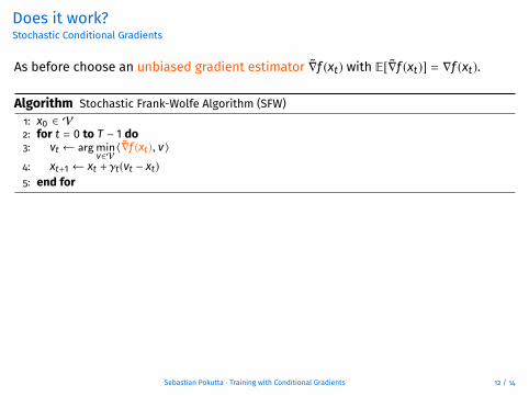
Does it work?Stochastic Conditional Gradients
As before choose an unbiased gradient estimator ∇̃f (xt) with E[∇̃f (xt)] = ∇f (xt).
Algorithm Stochastic Frank-Wolfe Algorithm (SFW)1: x0 ∈ V2: for t = 0 to T − 1 do3: vt ← argmin
v∈V〈∇f (xt), v〉
4: xt+1 ← xt + γt(vt − xt)5: end for
Similarly, many variants available• Batch versions. Rather than just taking one stochastic gradient, sample andaverage a mini batch. This also reduces variance of the gradient estimator.• Learning rate schedules. To ensure convergence the learning rate η is dynamicallymanaged.• Variance Reduction. Compute exact gradient once in a while as reference point,e.g., SVRF, SVRCGS, ...
Sebastian Pokutta · Training with Conditional Gradients 12 / 14
Does it work?Stochastic Conditional Gradients
As before choose an unbiased gradient estimator ∇̃f (xt) with E[∇̃f (xt)] = ∇f (xt).
Algorithm Stochastic Frank-Wolfe Algorithm (SFW)1: x0 ∈ V2: for t = 0 to T − 1 do3: vt ← argmin
v∈V〈∇̃f (xt), v〉
4: xt+1 ← xt + γt(vt − xt)5: end for
Similarly, many variants available• Batch versions. Rather than just taking one stochastic gradient, sample andaverage a mini batch. This also reduces variance of the gradient estimator.• Learning rate schedules. To ensure convergence the learning rate η is dynamicallymanaged.• Variance Reduction. Compute exact gradient once in a while as reference point,e.g., SVRF, SVRCGS, ...
Sebastian Pokutta · Training with Conditional Gradients 12 / 14

Does it work?Stochastic Conditional Gradients
As before choose an unbiased gradient estimator ∇̃f (xt) with E[∇̃f (xt)] = ∇f (xt).
Algorithm Stochastic Frank-Wolfe Algorithm (SFW)1: x0 ∈ V2: for t = 0 to T − 1 do3: vt ← argmin
v∈V〈∇̃f (xt), v〉
4: xt+1 ← xt + γt(vt − xt)5: end for
Similarly, many variants available• Batch versions. Rather than just taking one stochastic gradient, sample andaverage a mini batch. This also reduces variance of the gradient estimator.
• Learning rate schedules. To ensure convergence the learning rate η is dynamicallymanaged.• Variance Reduction. Compute exact gradient once in a while as reference point,e.g., SVRF, SVRCGS, ...
Sebastian Pokutta · Training with Conditional Gradients 12 / 14

Does it work?Stochastic Conditional Gradients
As before choose an unbiased gradient estimator ∇̃f (xt) with E[∇̃f (xt)] = ∇f (xt).
Algorithm Stochastic Frank-Wolfe Algorithm (SFW)1: x0 ∈ V2: for t = 0 to T − 1 do3: vt ← argmin
v∈V〈∇̃f (xt), v〉
4: xt+1 ← xt + γt(vt − xt)5: end for
Similarly, many variants available• Batch versions. Rather than just taking one stochastic gradient, sample andaverage a mini batch. This also reduces variance of the gradient estimator.• Learning rate schedules. To ensure convergence the learning rate η is dynamicallymanaged.
• Variance Reduction. Compute exact gradient once in a while as reference point,e.g., SVRF, SVRCGS, ...
Sebastian Pokutta · Training with Conditional Gradients 12 / 14

Does it work?Stochastic Conditional Gradients
As before choose an unbiased gradient estimator ∇̃f (xt) with E[∇̃f (xt)] = ∇f (xt).
Algorithm Stochastic Frank-Wolfe Algorithm (SFW)1: x0 ∈ V2: for t = 0 to T − 1 do3: vt ← argmin
v∈V〈∇̃f (xt), v〉
4: xt+1 ← xt + γt(vt − xt)5: end for
Similarly, many variants available• Batch versions. Rather than just taking one stochastic gradient, sample andaverage a mini batch. This also reduces variance of the gradient estimator.• Learning rate schedules. To ensure convergence the learning rate η is dynamicallymanaged.• Variance Reduction. Compute exact gradient once in a while as reference point,e.g., SVRF, SVRCGS, ...
Sebastian Pokutta · Training with Conditional Gradients 12 / 14

Does it work?Stochastic Conditional Gradients
Same setup as before. SGD and SFW as solvers.
test set accuracyFrank Wolfe Gradient Descent
0 20 40 60 80 100
epoch0.2
0.3
0.4
0.5
0.6
0.7
0.8
test set accuracy with noise (σ = 0.3)Frank Wolfe Gradient Descent
0 20 40 60 80 100
epoch0.2
0.3
0.4
0.5
0.6
0.7
0.8
test set accuracy with noise (σ = 0.6)Frank Wolfe Gradient Descent
0 20 40 60 80 100
epoch0.2
0.3
0.4
0.5
0.6
0.7
0.8
Performance for Neural Network trained on MNIST.
More details and experiments in the exercise...
Sebastian Pokutta · Training with Conditional Gradients 13 / 14

Thank you!
Sebastian Pokutta · Training with Conditional Gradients 14 / 14
Related Documents
![A Dynamic Conditional Random Field Model for Joint ... · [4]Navneet Dalal and Bill Triggs. Histograms of oriented gradients for human detection. In CVPR, 2005. [5]Xuming He, Richard](https://static.cupdf.com/doc/110x72/60049d4c8966990be21d6342/a-dynamic-conditional-random-field-model-for-joint-4navneet-dalal-and-bill.jpg)