Robust goal-oriented error estimation based on the constitutive relation error for stochastic problems

Robust goal-oriented error estimation based on the

constitutive relation error for stochastic problems

Ludovic Chamoin a, Eric Florentin a,∗, Sylvain Pavot a, Vincent Visseq b

a LMT-Cachan (ENS Cachan/CNRS/Paris 6 Univ./PRES UniverSud Paris)

61 Avenue du President Wilson, 94235 CACHAN Cedex, France

b Laboratoire de Mecanique et Genie Civil (LMGC) , UMR5508 CNRS / Universite Montpellier 2

CC048, Place E. Bataillon, 34095 Montpellier Cedex 5 - France

Abstract

In this paper, we aim at extending to stochastic models a general and robust goal-oriented error estimation method

presented in previous works. This method, which is based on the constitutive relation error and classical extraction

techniques, enables to obtain strict bounds on quantities of interest. In the stochastic framework, several aspects

are revisited in the current paper:(i) the construction of admissible fields, which is a pillar of the constitutive

relation error; (ii) the error bounding itself; (iii) the splitting of error sources that may enable to drive adaptive

procedures effectively. Performances of the proposed approach are illustrated on two-dimensional applications.

Key words: model verification, stochastic models, goal-oriented error estimation, strict bounds

Preprint submitted to Computers and Structures 8 mai 2012

1. Introduction

In the design of engineering components and structures, critical decisions are being more and more

based on the results coming from finite element analyses. Therefore, in order to develop confidence in

such decisions, controlling the quality of numerical simulations has become a vital issue in both research

and industry. This research topic, referred to as model verification, has been extensively studied for more

than thirty years and has led to the emergence of powerful methods, particularly as regards the assessment

of the global discretization error (see [1,18] for an overview). More recently, research has focused on goal-

oriented error estimation, i.e. the estimation of the error on specific outputs of interest which may be

relevant for design purposes. Several techniques have been proposed for goal-oriented error estimation,

and particularly for linear problems [28,7,30,34,38,10]. However, only few of these actually lead to strict

error bounds.

A general framework was recently introduced for robust goal-oriented error estimation ; it has the ad-

vantage to be valid for a large class of mechanical problems [17,22]. This framework, based on the concept

of constitutive relation error, in association with extraction techniques (that require the solution of an

adjoint problem), enables the calculation of strict and accurate bounds on the local error. The method has

been recently and successfully applied to various problems such as fracture mechanics tackled with XFEM

[27], (visco-)elasticity [5], transient viscodynamics [21], or (visco-)plasticity. In [6,22], a non-intrusive ap-

proach was also added to this framework in order to solve the adjoint problem in an optimal manner,

which enables in particular to consider pointwise quantities of interest in time and space. This powerful

approach consists in a local enrichment of the adjoint solution, using pre-computed generalized Green’s

functions, in order to catch effectively and at reasonable cost the locally irregular aspects of this solution.

∗. Corresponding author

Email addresses: [email protected] (Ludovic Chamoin), [email protected] (Eric Florentin),

[email protected] (Sylvain Pavot), [email protected] (Vincent Visseq).

2

During the last decade, with the fast increase of computing resources, complex models involving stochas-

tic parameters have been introduced in the computational mechanics community. Such models, which are

more and more employed and simulated nowadays [13,36,24,9,37,2], enable to represent lacks of know-

ledge in the modeling process as well as intrinsic physical randomness. As regards the verification of

stochastic models, most of the works are devoted to global error estimation (see [14,16] for instance). For

goal-oriented error estimation, the proposed methods [26,19,12] apply to a specific set of quantities of

interest and do not yield strict error bounds (only error indicators obtained through heuristic arguments).

In this work, we aim at extending the previously introduced general goal-oriented error estimation me-

thod to stochastic mechanical models. In order to do so, a first key point to consider is the construction,

in a stochastic sense, of an admissible solution which is required to apply the constitutive relation error ;

this point was first addressed in [16]. Furthermore, we need to extend the bounding result obtained for

the local error. A third point should deal with the splitting of error sources (i.e. error contributions due

to discretizations in space and stochastic dimensions in our case), and assessment of these contributions

in order to drive adaptive algorithms effectively, if necessary [11].

Consequently, the paper is structured as follows : after this introduction, Section 2 describes the sto-

chastic reference problem we consider throughout the paper, and gives details about the computation of

an associated approximate solution ; Section 3 recalls, for the stochastic framework, the main features of

the constitutive relation error and the construction of an admissible solution ; Section 4 introduces the

stochastic version of the goal-oriented error estimation method we use, as well as the procedure employed

to estimate contributions of various error sources ; numerical results are presented in Section 5 ; eventually,

conclusions and prospects are drawn in Section 6.

3

2. Reference problem and notations

2.1. The stochastic reference problem

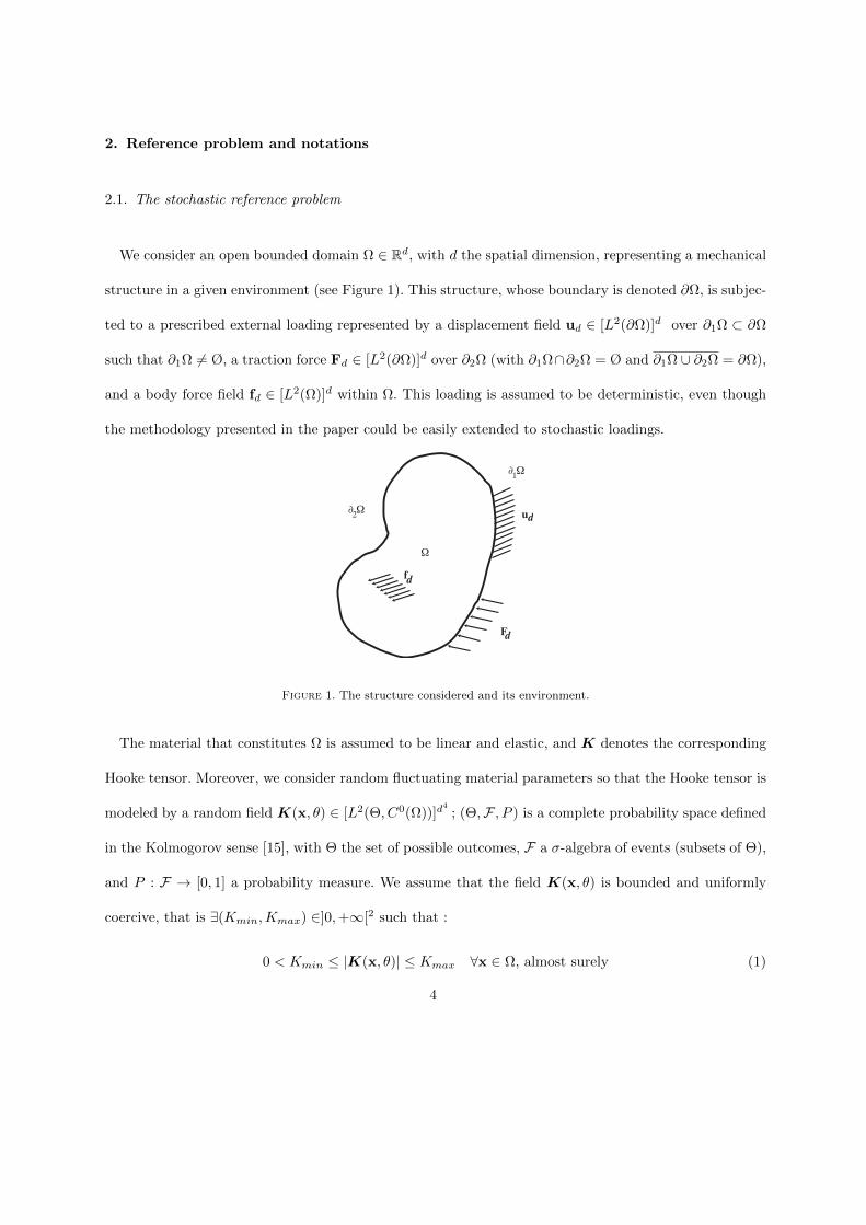
We consider an open bounded domain Ω ∈ Rd, with d the spatial dimension, representing a mechanical

structure in a given environment (see Figure 1). This structure, whose boundary is denoted ∂Ω, is subjec-

ted to a prescribed external loading represented by a displacement field ud ∈ [L2(∂Ω)]d over ∂1Ω ⊂ ∂Ω

such that ∂1Ω 6= Ø, a traction force Fd ∈ [L2(∂Ω)]d over ∂2Ω (with ∂1Ω∩∂2Ω = Ø and ∂1Ω ∪ ∂2Ω = ∂Ω),

and a body force field fd ∈ [L2(Ω)]d within Ω. This loading is assumed to be deterministic, even though

the methodology presented in the paper could be easily extended to stochastic loadings.

F

ud

d

Ω

∂ Ω2

∂ Ω1

df

Figure 1. The structure considered and its environment.

The material that constitutes Ω is assumed to be linear and elastic, and K denotes the corresponding

Hooke tensor. Moreover, we consider random fluctuating material parameters so that the Hooke tensor is

modeled by a random field K(x, θ) ∈ [L2(Θ, C0(Ω))]d4

; (Θ,F , P ) is a complete probability space defined

in the Kolmogorov sense [15], with Θ the set of possible outcomes, F a σ-algebra of events (subsets of Θ),

and P : F → [0, 1] a probability measure. We assume that the field K(x, θ) is bounded and uniformly

coercive, that is ∃(Kmin,Kmax) ∈]0,+∞[2 such that :

0 < Kmin ≤ |K(x, θ)| ≤ Kmax ∀x ∈ Ω, almost surely (1)

4

Remark 1 Following the Karhunen-Loeve expansion [23], the stochastic description of K will be limited

to a finite number of M uncorrelated stochastic variables ξk(θ) : Θ→ R such that :

K(x, θ) ≈ K(x) +

M∑k=1

√λkξk(θ)Zk(x) (2)

where K =∫

ΘKdP is the mean value of K, whereas Zk, λk are eigenvector/eigenvalue pairs of the

covariance operator. This truncation at order M provides for an approximation of K.

We equip the space (Θ,F , P ) with an L2-inner product on probability measures, defined as :

〈α, β〉 ≡∫

Θ

α(θ)β(θ)dP (θ) (3)

where (α, β) is a couple of random variables and dP is the probability measure of θ. We also define the

following norms on Ω×Θ :

||| • |||K =

(E[∫

Tr["(•)K"(•)]dΩ

])1/2

=(E[|| • ||2K

])1/2||| • |||K−1 =

(E[∫

Tr[•K−1•]dΩ

])1/2

=(E[|| • ||2K−1

])1/2 (4)

where E(•) =∫

Θ• dP is the mathematical expectation of •.

Assuming an isothermal state with small perturbations, the quasi-static problem consists of finding the

displacement-stress pair (u(x, θ),(x, θ)) which verifies :

• the kinematic compatibility equations :

u ∈ U ; u|∂1Ω = ud almost surely (5)

• the equilibrium equations :

∈ S ; E[∫

Ω

Tr["(u∗)]dΩ−∫

Ω

fd · u∗dΩ−∫∂2Ω

Fd · u∗dS]

= 0 ∀u∗ ∈ U0 (6)

• the constitutive relation :

= K"(u) (7)

where U = [L2(Θ, H1(Ω))]d, S =τ ; τ = τT , τ ∈ [L2(Θ, L2(Ω))]d

2

, and U0 is the vectorial space asso-

ciated with U . "(•) = 12 [Grad•+ GradT •] is the linearized strain tensor.

5

2.2. Discretization errors

The exact solution of problem (5–7) is denoted (uex,ex). In practice, it is approximated using a

stochastic finite element method (SFEM) [39]. In the space dimension, we use a discretization of Ω, based

on mesh Mh. In the stochastic dimension, the discretization used for Θ is based on a grid Mm. Two

families of techniques exist :

– non-intrusive techniques, such as Monte Carlo methods or regression methods, in which a set of

events is drawn to compute realizations in a deterministic way ;

– intrusive techniques, such as the (generalized) Polynomial Chaos associated with the stochastic finite

element method, which search an approximate solution in a finite dimension space.

In both cases, polynomial chaos is often used for Mm. This space is defined from a polynomial ba-

sis ΨiLi=1 of variables ξk(θ)Mk=1. Namely, elements of the basis are defined as Ψi ( ξk(θ)Mk=1

)=∏M

k=1Hk,i(ξk), where Hk,i(ξk) are orthonormal polynomials with respect to the inner-product defined

in (3). A review on these various possible techniques that yield approximate stochastic solutions can be

found in [4]. In the following, and without loss of generality, we consider a non-intrusive technique based

on interpolation, over the stochastic domain, of a given number of computed realizations. More precisely,

L deterministic simulations are performed and lead to displacement fields uih(x) (i = 1, . . . , L). The sto-

chastic field uh,m(x, θ) is then obtained after interpolation using shape functions Ψi (i = 1, . . . , L) ; uh,m

then reads :

uh,m(x, θ) =

L∑i=1

uih(x).Ψi ( ξk(θ)Mk=1

)=

L∑i=1

uih(x).Ψi (θ) (8)

The approximated solution is denoted (uh,m,h,m), where h,m = K"(uh,m). Subscript h (resp. m)

denotes the discretization in the space (resp. stochastic) dimension related to meshMh (resp. gridMm).

Using then the energetic norm associated to operator K, we define a measure of the global discretization

6

error :

Eglob = |||uex − uh,m|||K (9)

We can also define the discretization error on a quantity of interest I(u) representing a specific feature

of the global solution u :

Eloc = I(uex)− I(uh,m) = Iex − Ih,m (10)

Such a quantity of interest could be the mean of a component of the displacement or stress on a given

zone.

3. Constitutive relation error

3.1. Definition and properties

We first introduce the notion of admissibility for a displacement-stress pair. A solution (u, ) ∈ U × S

is said admissible if u verifies (5) and verifies (6). We will show in Section 3.2 that such a solution can

be obtained as a post-processing of (uh,m,h,m).

We then define, for an admissible couple (u, ), the constitutive relation error in a stochastic sense :

ecre(u, ) = ||| −K"(u)|||K−1 ≥ 0 (11)

This is a straightforward generalization of the classical constitutive relation error given for deterministic

models [18] :

ecre,spa(u, ) = || −K"(u)||K−1 (12)

It is also easy to show that properties of this latter constitutive relation error (see [18]) extend to the

stochastic formulation :

ecre(u, ) = 0⇐⇒ (u, ) = (uex,ex) almost surely (13)

e2cre(u, ) = |||uex − u|||2K + |||ex − |||2K−1 (14)

7

e2cre(u, ) = 4 |||ex −

∗|||2K−1 (15)

with ∗ = 1

2 [ + K"(u)].

3.2. Computation of admissible fields

An admissible solution, denoted (uh,m, h,m) in the following, is computed from the approximate solu-

tion (uh,m,h,m) at hand. On the one hand, as regards the kinematically admissible displacement field

uh,m, we merely choose uh,m = uh,m even though other choices would be possible. On the other hand,

the computation of a statically admissible stress field h,m is a technical point of the method. It can be

performed using various techniques [18,8,20,25,29,33] ; here, we use the technique recently introduced in

[20] which constitutes a good compromise between quality and computational cost [31,32]. The practical

construction of h,m from h,m is detailed below.

• Direct construction : not admissible

The finite element stress field is generally post-treated as :

h,m(x, θ) =

L∑i=1

ih(x).Ψi (θ) (16)

Starting from components ih,m(x), it is possible to construct the associated admissible stress fields

ih,m(x) using directly techniques developed in the deterministic framework (see [31,32] for more details).

h,m(x, θ) =

L∑i=1

ih,m(x).Ψi (θ) (17)

The problem is that h,m(x, θ) is not admissible in the general case, as it does not respect (6), i.e. the

equilibrium equations over the whole space Θ.

• Definition of M′

m :

8

To avoid the previous problem, and enable a systematic construction of admissible field h,m(x, θ), we

introduce a dedicated basis. Generally, fd and Fd are chosen linear with random variables : we introduce

here a piecewise linear grid . If other choices are made for fd or Fd, a compatible basis can then be chosen.

We introduce the grid M′

m based on the same nodes as Mm but using multi-linear shape functions

χiLi=1. The L multilinear shape functions of the M random variables are defined by : χi ( ξk(θ)Mk=1

)=∏M

k=1Nk,i(ξk), where Nk,i(ξk) are the classical finite element unidimensional shape function relative to

ξk.

We denote Ph,m the representation of h,m defined on M′

h :

Ph,m(x, θ) =

L∑i=1

χi

h (x).χi ( ξk(θ)Mk=1

)=

L∑i=1

χi

h (x).χi (θ) (18)

where χi

h,m are components of the stress Ph,m on χi.

Then components Nih (x) of the stress h,m(x, θ) in the basis χi can be computed directly using the

different techniques developed in deterministic framework from components χi

h (x) [31,32].

h,m(x, θ) =

L∑i=1

χi

h (x).χi (θ) (19)

The introduction of the basis χi is done to ensure the admissibility of h,m. Indeed, as far as

χi ( ξk(θ)Mk=1

)is a multi-linear function of the M variables ξk(θ)Mk=1 , any linear combination of

admissible stress fields χi

h (x) (by deterministic construction) will remain admissible. The only assump-

tion to make is that the loading remains linear with random variables ξk(θ)Mk=1 (which is not a strong

assumption . . .).

9

4. Goal-oriented error estimation

4.1. Adjoint problem

Assuming it is linear with respect to u, the quantity of interest I is first written under the global form :

I =

∫Θ

∫Ω

Tr[Σ"(u)] + fΣ · u

dΩdP (20)

where stress field Σ(x, θ) and body force field fΣ(x, θ), which may be explicitly or implicitly given, are

extractors defined on Ω×Θ.

Using the optimal control approach proposed in [3], we define the adjoint problem related to I ; it

consists of finding the displacement-stress pair (u(x, θ), (x, θ)) which verifies :

• the kinematic compatibility equations :

u ∈ U ; u|∂1Ω = 0 almost surely (21)

• the equilibrium equations :

∈ S ; E[∫

Ω

Tr[( − Σ)"(u∗)]dΩ−∫

Ω

fΣ · u∗dΩ

]= 0 ∀u∗ ∈ U0 (22)

• the constitutive relation :

= K"(u) (23)

As for the primal problem, we compute an approximate displacement-stress pair (uh,m(x, θ), h,m(x, θ))

using the same mesh Mh and grid Mm.

We also derive an admissible displacement-stress pair(

ˆuh,m(x, θ), ˆh,m(x, θ))

using the same tech-

niques as for the primal problem.

10

4.2. Error bounding

From quantities previously computed for primal and adjoint problems, we obtain the fundamental

relation :

Eloc = Iex − Ih,m = E[∫

Ω

Tr[(ˆh,m −K"(ˆuh,m))K−1(ex − h,m)]dΩ

](24)

This result, for which proof can be found in [17,22], shows that local error Eloc can be represented from

global solutions of both reference and adjoint problems.

From (24), and using the Cauchy-Schwarz inequality, we eventually obtain the guaranteed upper bound

Eloc on the local error Eloc :

|Eloc| ≤ Eloc (25)

with :

Eloc = ecre(u, ) · ecre(ˆu, ˆ) (26)

The bound Eloc is easy to implement (analytical computations may be possible) and the error on primal

and adjoint solutions can be computed separately.

4.3. Splitting of error sources

In the problem we consider, the discretization error Iex − Ih,m on a given quantity of interest I comes

from two sources : (i) discretization of the space domain using a finite element mesh ; (ii) discretization

of the stochastic domain. In this section, we aim at assessing contributions of these two sources, in order

to get relevant information that would help for driving adaptive procedures. The local error can be recast

under the form :

Eloc = [Iex − Ih] + [Ih − Ih,m] = Eloc,spa + Eloc,sto (27)

11

where Ih is the quantity of interest, corresponding to an exact resolution regarding randomness, but with

a discretized solution using Mh regarding space. That way, Eloc,spa (resp. Eloc,sto) is the contribution of

the discretization error on I due to the discretization of the space dimension (resp. stochastic dimension).

On the one hand, contribution Eloc,sto = Ih − Ih,m can be estimated using the goal-oriented error

estimation method described previously, provided that the reference model which is considered is already

discretized in space, i.e. taking the reference problem defined in Section 2.1 and applying a finite element

discretization to it. With respect to this new reference problem, Ih is the exact solution, and Ih,m is an

approximate solution obtained after discretization in the stochastic dimension.

In that framework, an admissible displacement/stress pair denoted (um, m) shall be defined relative

to this new reference model. In practice, such a pair can be automatically obtained as a simple post-

processing of the approximate solution (uh,m,h,m) at hand : we take um = uh,m, and construct m

as :

m(x, θ) =

L∑i=1

χi

h (x).χi (θ) (28)

The construction of admissible fields (ˆum, ˆm) for the new adjoint problem is similar. We eventually ob-

tain the estimate Eloc,sto = ecre(um, m) · ecre(ˆum, ˆm), which is a guaranteed upper bound on the error

|Ih − Ih,m|.

In the same way, contribution Eloc,spa = Iex − Ih ≈ Im − Ih,m can be estimated taking as the reference

model the one defined in Section 2.1 on which we apply the discretization in the stochastic dimension.

With respect to this new reference problem, Im is the exact solution, and Ih,m is an approximate solution

obtained after discretization in the space dimension. An admissible displacement/stress pair denoted

(uh, h), and relative to this new reference model, is again obtained as a simple post-processing of the

approximate solution (uh,m,h,m) at hand : we take uh = uh,m, and construct h as :

12

h(x, θ) =

L∑i=1

ih,m(x).Ψi (θ) (29)

The construction of admissible fields (ˆuh, ˆh) for the new adjoint problem is similar. We eventually ob-

tain the estimate Eloc,spa = ecre(uh, h) · ecre(ˆuh, ˆh), which is a guaranteed upper bound on the error

|Im − Ih,m|.

5. Numerical results

5.1. Test problems

Two test-problems are considered here ; the first (denoted [A]) is illustrated in Figure 2, the second

(denoted [B]) is illustrated in Figure 3. In both problems, Young’s modulus E1 is partially known in zone

Ω1 ; we assume that this random variable (defined on Ω1) has a given probability density with mean E1

and variation δ1 :

E1(θ) = E1. [1 + δ1g (ξ(θ))] with g(x) =2 arcsin(Erf( x√

2))

√π2 − 8

(30)

where ξ(θ) is a Gaussian centered random variable. The nonlinear function g is introduced, such that the

probability density function E1(θ) as a bounded support (this definition avoids negative Young’s modulus

values which would not be physically correct). The Young modulus E2 is deterministic in zone Ω2.

On problem [A] the gamma shape structure is submitted to a given traction force F xd along x axis and

to a prescribed displacement uyd along y axis and is clamped on the bottom boundary. On problem [B],

the square structure is clamped on bottom and top boundaries, and submitted to prescribed displacement

uyd along y axis.

Data, loading, material, and geometry parameters are given in Table 1 for problems [A] and [B].

13

u

FP

O

x

y

b

d

a

c

Figure 2. Definition of problem [A] : Gamma shape structure with clamped bottom boundary, prescribed displacement uyd

on top boundary, and prescribed traction Fxd on top-right boundary.

FP

O

x

y

b

c

a

Figure 3. Definition of problem [B] : Square structure with clamped bottom and top boundaries, and prescribed traction

Fxd on top-right boundary.

In both problems, the studied quantity of interest is the mean horizontal displacement on the application

zone of Fd. More precisely :

I =

∫Θ

∫Ω

fΣ · u dΩdP (31)

with :

14

E1 δ1 E2 Fxd uy

da b c d

[A] 1 0.1 2 −1.5 −2 25 20 10 10

[B] 1 0.2 2 2 - 10 10 5 -

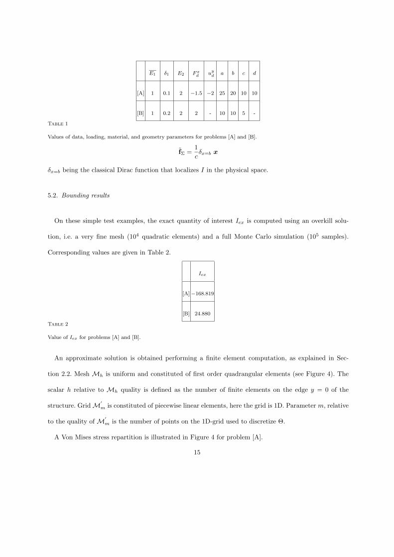
Table 1

Values of data, loading, material, and geometry parameters for problems [A] and [B].

fΣ =1

cδx=b x

δx=b being the classical Dirac function that localizes I in the physical space.

5.2. Bounding results

On these simple test examples, the exact quantity of interest Iex is computed using an overkill solu-

tion, i.e. a very fine mesh (104 quadratic elements) and a full Monte Carlo simulation (105 samples).

Corresponding values are given in Table 2.

Iex

[A] −168.819

[B] 24.880

Table 2

Value of Iex for problems [A] and [B].

An approximate solution is obtained performing a finite element computation, as explained in Sec-

tion 2.2. Mesh Mh is uniform and constituted of first order quadrangular elements (see Figure 4). The

scalar h relative to Mh quality is defined as the number of finite elements on the edge y = 0 of the

structure. GridM′

m is constituted of piecewise linear elements, here the grid is 1D. Parameter m, relative

to the quality of M′

m is the number of points on the 1D-grid used to discretize Θ.

A Von Mises stress repartition is illustrated in Figure 4 for problem [A].

15

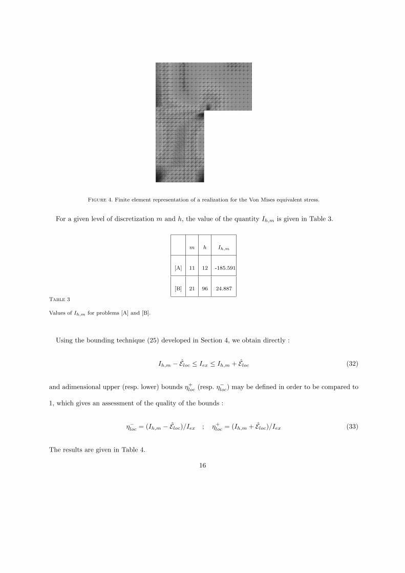
Figure 4. Finite element representation of a realization for the Von Mises equivalent stress.

For a given level of discretization m and h, the value of the quantity Ih,m is given in Table 3.

m h Ih,m

[A] 11 12 -185.591

[B] 21 96 24.887

Table 3

Values of Ih,m for problems [A] and [B].

Using the bounding technique (25) developed in Section 4, we obtain directly :

Ih,m − Eloc ≤ Iex ≤ Ih,m + Eloc (32)

and adimensional upper (resp. lower) bounds η+loc (resp. η−loc) may be defined in order to be compared to

1, which gives an assessment of the quality of the bounds :

η−loc = (Ih,m − Eloc)/Iex ; η+loc = (Ih,m + Eloc)/Iex (33)

The results are given in Table 4.

16

Ih,m − Eloc Iex Ih,m − Eloc η−loc

η+loc

[A] -207.863 -168.819 -163.319 0.9674 1.2313

[B] 24.812 24.807 24.966 0.997 1.003

Table 4

Bounds on Iex for problems [A] and [B].

5.3. Refinement of the discretization

In this section we present the evolution of the adimensional bounds with respect to the refinement of

the space mesh (i.e. variation of parameter h), and the refinement of the grid (i.e. variation of parameter

m). In Table 5, we give the different values of the adimensional bounds for different space mesh qualities

h, m being fixed, for problem [A]. In Table 6, we give the different values of the adimensional bounds for

different mesh grid qualities m, h being fixed, for problem [A].

m h Ih,m Eloc η−loc

η+loc

11 6 −154.087 62.420 0.542 1.282

11 12 −163.188 22.275 0.834 1.098

11 24 −165.898 7.456 0.938 1.026

11 48 −166.997 2.554 0.974 1.004

11 72 −168.272 1.395 0.988 1.005

Table 5

Evolution of the bounds with respect to the refinement of the space mesh size for problem [A].

In Table 7, we give the different values of the adimensional bounds for different space mesh qualities

h, m being fixed, for problem [B]. In Table 8, we give the different values of the adimensional bounds for

different mesh grid qualities m, h being fixed, for problem [B].

17

m h Ih,m Eloc η−loc

η+loc

3 12 -161.869 23.791 0.817 1.099

5 12 -162.911 22.527 0.831 1.098

11 12 -163.188 22.271 0.834 1.098

21 12 -162.714 22.218 0.832 1.095

41 12 -162.717 22.193 0.832 1.095

81 12 -162.718 22.180 0.832 1.095

Table 6

Evolution of the bounds with respect to the refinement of the grid size for problem [A].

m h Ih,m Eloc η−loc

η+loc

3 12 24.166 2.818 0.858 1.084

3 24 24.668 0.963 0.952 1.030

3 48 24.852 0.328 0.985 1.012

3 96 24.921 0.130 0.996 1.006

3 144 24.940 0.086 0.998 1.005

Table 7

Evolution of the bounds with respect to the refinement of the space mesh size for problem [B].

5.4. Estimation of contributions of various error sources

We are now interested in the estimating parts of the error due to the stochastic (resp. space) discreti-

zation Eloc,sto (resp. Eloc,spa) as explained in Section 4.3. For different values of h and m, the results are

given in Tables 9 and 10 (resp. Tables 11 and 12) for problem [A] (resp. problem [B]).

18

m h Ih,m Eloc η−loc

η+loc

3 96 24.921 0.130 0.996 1.007

5 96 24.895 0.084 0.997 1.004

11 96 24.893 0.080 0.997 1.004

21 96 24.887 0.079 0.997 1.003

41 96 24.881 0.078 0.997 1.003

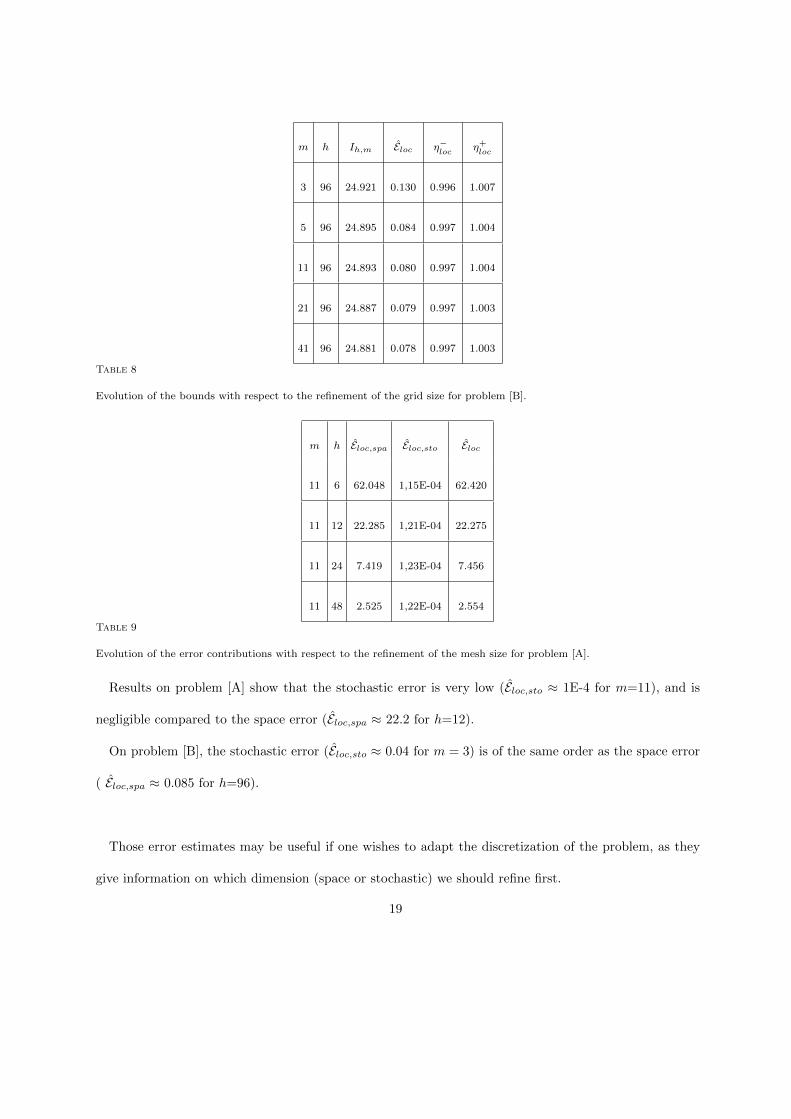
Table 8

Evolution of the bounds with respect to the refinement of the grid size for problem [B].

m h Eloc,spa Eloc,sto Eloc

11 6 62.048 1,15E-04 62.420

11 12 22.285 1,21E-04 22.275

11 24 7.419 1,23E-04 7.456

11 48 2.525 1,22E-04 2.554

Table 9

Evolution of the error contributions with respect to the refinement of the mesh size for problem [A].

Results on problem [A] show that the stochastic error is very low (Eloc,sto ≈ 1E-4 for m=11), and is

negligible compared to the space error (Eloc,spa ≈ 22.2 for h=12).

On problem [B], the stochastic error (Eloc,sto ≈ 0.04 for m = 3) is of the same order as the space error

( Eloc,spa ≈ 0.085 for h=96).

Those error estimates may be useful if one wishes to adapt the discretization of the problem, as they

give information on which dimension (space or stochastic) we should refine first.

19

m h Eloc,spa Eloc,sto Eloc

3 12 22.181 0.174 23.791

5 12 22.311 0.004 22.527

11 12 22.285 1E-04 22.271

21 12 22.287 8E-06 22.218

41 12 22.287 4E-07 22.193

81 12 22.285 3E-08 22.180

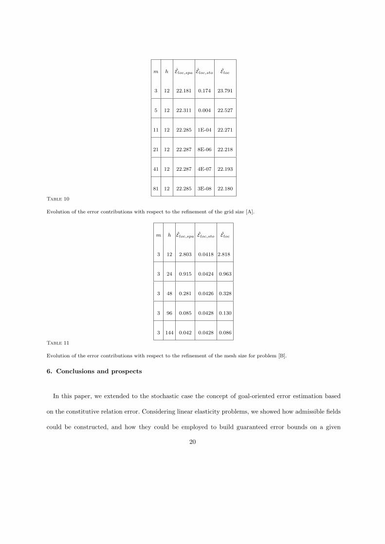
Table 10

Evolution of the error contributions with respect to the refinement of the grid size [A].

m h Eloc,spa Eloc,sto Eloc

3 12 2.803 0.0418 2.818

3 24 0.915 0.0424 0.963

3 48 0.281 0.0426 0.328

3 96 0.085 0.0428 0.130

3 144 0.042 0.0428 0.086

Table 11

Evolution of the error contributions with respect to the refinement of the mesh size for problem [B].

6. Conclusions and prospects

In this paper, we extended to the stochastic case the concept of goal-oriented error estimation based

on the constitutive relation error. Considering linear elasticity problems, we showed how admissible fields

could be constructed, and how they could be employed to build guaranteed error bounds on a given

20

m h Eloc,spa Eloc,sto Eloc

3 96 0.085 0.043 0.130

5 96 0.086 0.003 0.084

11 96 0.085 3.4E-04 0.080

21 96 0.085 2E-05 0.079

41 96 0.085 1E-06 0.078

Table 12

Evolution of the error contributions with respect to the refinement of the grid size [B].

quantity of interest. We also proposed a simple procedure to assess separately contributions coming from

various error sources (discretizations in space and stochastic dimensions in our case). The capabilities of

these new tools were illustrated on 2D numerical experiments.

In future works, we wish to tackle problems with a large number of stochastic variables. We also wish

to adapt to the stochastic case the non-intrusive procedure proposed in [6].

References

[1] Babuska I, Strouboulis T. The finite element method and its reliability. Oxford university press, 2001.

[2] Babuska I, Nobile F, Tempone R. A stochastic collocation method for elliptic partial differential equations with random

input data. SIAM Journal on Numerical Analysis 2007; 45(3):1005–1034.

[3] Becker R, Rannacher R. An optimal control approach to shape a posteriori error estimation in finite element methods.

A. Isereles (Ed.), Acta Numerica,Cambridge University Press, 2001; 10:1–120.

[4] Berveiller M. Stochastic finite elements: intrusive and non-intrusive methods for reliability analysis. PhD thesis,

Universite Blaise Pascal 2005.

[5] Chamoin L, Ladeveze P. Bounds on history-dependent or independent local quantities in viscoelasticity problems solved

by approximate methods. International Journal for Numerical Methods in Engineering 2007; 71(12):1387–1411.

21

[6] Chamoin L, Ladeveze P. A non-intrusive method for the calculation of strict and efficient bounds of calculated outputs

of interest in linear viscoelasticity problems. Computer Methods in Applied Mechanics and Engineering 2008; 197(9-

12):994–1014.

[7] Cirak F, Ramm E. A posteriori error estimation and adaptivity for linear elasticity using the reciprocal theorem.

Computer Methods in Applied Mechanics and Engineering 1998; 156:351–362.

[8] Cottereau R, Diez P, Huerta A. Strict error bounds for linear solid mechanics problems using a subdomain-based

flux-free method. Computational Mechanics 2009; 44(4):533–547.

[9] Deb M.K, Babuska I, Oden J.T. Solution of stochastic partial differential equations using Galerkin finite element

techniques. Computer Methods in Applied Mechanics and Engineering 2001; 190:6359–6372.

[10] Florentin E, Gallimard L, Pelle J.P. Evaluation of the local quality of stresses in 3D finite element analysis. Computer

Methods in Applied Mechanics and Engineering 2002; 191:4441–4457.

[11] Florentin E, Gallimard L, Pelle J.P, Rougeot Ph. Adaptive meshing for local quality of FE stresses. Engineering

Computations 2005; 22:149–164.

[12] Florentin E, Ladeveze P, Bellec J. Error bounds on outputs of interest for linear stochastic problems. in Proceedings

of the 3rd European Conference on Computational Mechanics 2006.

[13] Ghanem R, Spanos P.D. Stochastic Finite Elements: A Spectral Approach. Springer Verlag, 1991.

[14] Ghanem R, Pelissetti M. Error estimation for the validation of model-based predictions. in Proceedings of the 5th

World Congress on Computational Mechanics 2002.

[15] Kolmogorov A.N. Foundations of the Theory of Probability. Chelsea Publishing Company, New York, 1956.

[16] Ladeveze P. Validation and verification of stochastic models in uncertain environment using constitutive relation error

method. Technical Report 258, LMT-Cachan 2003.

[17] Ladeveze P. Strict upper error bounds for calculated outputs of interest in computational structural mechanics.

Computational Mechanics 2008; 42(2):271–286.

[18] Ladeveze P, Pelle J-P. Mastering Calculations in Linear and Nonlinear Mechanics. Springer NY, 2004.

[19] Ladeveze P, Florentin E. Verification of stochastic models in uncertain environments using the constitutive relation

error method. Computer Methods in Applied Mechanics and Engineering 2006; 196:225–234.

22

[20] Ladeveze P, Chamoin L, Florentin E. A new non-intrusive technique for the construction of admissible stress fields in

model verification. Computer Methods in Applied Mechanics and Engineering; 2010; 199(9-12):766–777.

[21] Ladeveze P, Waeytens J. Model verification in dynamics through strict upper error bounds. Computer Methods in

Applied Mechanics and Engineering 2009; 198(21-26):1775–1784.

[22] Ladeveze P, Chamoin L. Calculation of strict error bounds for finite element approximations of non-linear pointwise

quantities of interest. International Journal for Numerical Methods in Engineering; 2010; 84:1638–1664.

[23] Loeve M. Probability Theory (4th edition). Springer-Verlag, Berlin, 1977.

[24] Matthies H.G, Bucher C.G. Finite element for stochastic media problems. Computer Methods in Applied Mechanics

and Engineering 1999; 168:3–17.

[25] Moitinho de Almeida J.P, Maunder E.A.W. Recovery of equilibrium on star patches using a partition of unity technique.

International Journal for Numerical Methods in Engineering 2009; 79:1493–1516.

[26] Oden J.T, Babuska I, Nobile F, Feng Y, Tempone R. Theory and methodology for estimation and control of error

due to modeling, approximation, and uncertainty. Computer Methods in Applied Mechanics and Engineering 2005;

194:195–204.

[27] Panetier J, Ladeveze P, Chamoin L. Strict and effective bounds in goal-oriented error estimation applied to fracture

mechanics problems solved with XFEM. International Journal for Numerical Methods in Engineering 2010; 81:671–700.

[28] Paraschivoiu M, Peraire J, Patera A.T. A posteriori finite element bounds for linear functional outputs of elliptic partial

differential equations. Computer Methods in Applied Mechanics and Engineering 1997; 150:289–312.

[29] Pares N, Diez P, Huerta A. Subdomain-based flux-free a posteriori error estimators. Computer Methods in Applied

Mechanics and Engineering 2006; 195(4-6):297–323.

[30] Peraire J, Patera A.T. Bounds for linear-functional outputs of coercive partial differential equations; local indicators

and adaptive refinements. Advances in Adaptive Computational Methods in Mechanics (Ladeveze and Oden Editors,

Elsevier) 1998; 199–216.

[31] Pled F, Chamoin L, Ladeveze P. On the techniques for constructing admissible stress fields in model verification:

performances on engineering examples. International Journal for Numerical Methods in Engineering 2011; 88(5):409–

441.

23

[32] Florentin, E., Guinard S., Pasquet, P. A simple estimator for stress errors dedicated to large elastic finite element

simulations : Locally reinforced stress construction. Engineering Computations. 2011. 28:76-92

[33] Florentin E, Lubineau G. Identification of the parameters of an elastic material model using the Constitutive Equation

Gap Method. Computational Mechanics 2010; 46:521–531.

[34] Prudhomme S, Oden J.T. On goal-oriented error estimation for elliptic problems: application to the control of pointwise

errors. Computer Methods in Applied Mechanics and Engineering 1999; 176:313–331.

[35] Romkes A, Oden J.T, Vemaganti K. Multiscale goal-oriented adaptive modeling of random heterogeneous materials.

Mechanics of Materials 2006; 38:859–872.

[36] Schueller G. A state-of-the-art report on computational stochastic mechanics. Probabilistic Engineering Mechanics

1997; 12:197–321.

[37] Sudret B, Berveiller M, Lemaire M. Elements finis stochastiques en elasticite lineaire. Comptes Rendus de l’Academie

des Sciences, Mecanique 2004; 332:531–537.

[38] Stein E, Ohmnimus S, Walhorn E. Local error estimates of fem for displacements and stresses in linear elasticity by

solving local Neumann problems. International Journal for Numerical Methods in Engineering 2001; 52:727–746.

[39] Stefanou G. The stochastic finite element method: Past, present and future. Computer Methods in Applied Mechanics

and Engineering 2009; 198:1031–1051.

24