Robust Full Bayesian Learning for Radial Basis Networksnando/papers/neuralNetMCMC.pdf · Robust Full Bayesian Learning for Radial Basis Networks ... optimize neural networks. This

LETTER Communicated by Michael Jordan

Robust Full Bayesian Learning for Radial Basis Networks

Christophe Andrieu∗Cambridge University Engineering Department, Cambridge CB2 1PZ, England

Nando de FreitasComputer Science Division, University of California, Berkeley, CA 94720-1776, U.S.A.

Arnaud DoucetCambridge University Engineering Department, Cambridge CB2 1PZ, England

We propose a hierarchical full Bayesian model for radial basis networks.This model treats the model dimension (number of neurons), model pa-rameters, regularization parameters, and noise parameters as unknownrandom variables. We develop a reversible-jump Markov chain MonteCarlo (MCMC) method to perform the Bayesian computation. We findthat the results obtained using this method are not only better than theones reported previously, but also appear to be robust with respect tothe prior specification. In addition, we propose a novel and computation-ally efficient reversible-jump MCMC simulated annealing algorithm tooptimize neural networks. This algorithm enables us to maximize thejoint posterior distribution of the network parameters and the numberof basis function. It performs a global search in the joint space of the pa-rameters and number of parameters, thereby surmounting the problemof local minima to a large extent. We show that by calibrating the fullhierarchical Bayesian prior, we can obtain the classical Akaike informa-tion criterion, Bayesian information criterion, and minimum descriptionlength model selection criteria within a penalized likelihood framework.Finally, we present a geometric convergence theorem for the algorithmwith homogeneous transition kernel and a convergence theorem for thereversible-jump MCMC simulated annealing method.

1 Introduction

Buntine and Weigend (1991) and Mackay (1992) showed that a principledBayesian learning approach to neural networks can lead to many improve-ments. In particular, Mackay showed that by approximating the distribu-tions of the weights with gaussians and adopting smoothing priors, it is

∗ Authorship based on alphabetical order.

Neural Computation 13, 2359–2407 (2001) c© 2001 Massachusetts Institute of Technology

2360 C. Andrieu, N. de Freitas, and A. Doucet

possible to obtain estimates of the weights and output variances and to setthe regularization coefficients automatically.

Neal (1996) cast the net much further by introducing advanced Bayesiansimulation methods, specifically the hybrid Monte Carlo method (Brass,Pendleton, Chen, & Robson, 1993), into the analysis of neural networks. The-oretically, he also proved that certain classes of priors for neural networks,whose number of hidden neurons tends to infinity, converge to gaussianprocesses. Bayesian sequential Monte Carlo methods have also been shownto provide good training results, especially in time-varying scenarios (deFreitas, Niranjan, Gee, & Doucet, 2000).

An essential requirement of neural network training is the correct se-lection of the number of neurons. There have been three main approachesto this problem: penalized likelihood, predictive assessment, and grow-ing and pruning techniques. In the penalized likelihood context, a penaltyterm is added to the likelihood function so as to limit the number of neu-rons, thereby avoiding overfitting. Classical examples of penalty terms in-clude the well-known Akaike information criterion (AIC), Bayesian infor-mation criterion (BIC) and minimum description length (MDL) (Akaike,1974; Schwarz, 1985; Rissanen, 1987). Penalized likelihood has also beenused extensively to impose smoothing constraints by weight decay priors(Hinton, 1987; Mackay, 1992) or functional regularizers that penalize forhigh-frequency signal components (Girosi, Jones, & Poggio, 1995).

In the predictive assessment approach, the data are split into a trainingset, a validation set, and possibly a test set. The key idea is to balance thebias and variance of the predictor by choosing the number of neurons sothat the errors in each data set are of the same magnitude.

The problem with the previous approaches, known as the model ade-quacy problem, is that they assume one knows which models to test. Toovercome this difficulty, various authors have proposed model selectionmethods whereby the number of neurons is set by growing and pruning al-gorithms. Examples of this class of algorithms include the upstart algorithm(Frean, 1990), cascade correlation (Fahlman & Lebiere, 1988), optimal braindamage (Le Cun, Denker, & Solla, 1990) and the resource allocating network(RAN) (Platt, 1991). A major shortcoming of these methods is that they lackrobustness in that the results depend on several heuristically set thresholds.For argument’s sake, let us consider the case of the RAN algorithm. A newradial basis function is added to the hidden layer each time an input in anovel region of the input space is found. Unfortunately, novelty is assessedin terms of two heuristically set thresholds. The center of the gaussian basisfunction is then placed at the location of the novel input, while its widthdepends on the distance between the novel input and the stored patterns.For improved efficiency, the amplitudes of the gaussians may be estimatedwith an extended Kalman filter (Kadirkamanathan & Niranjan, 1993). Ying-wei, Sundararajan, and Saratchandran (1997) have extended the approachby proposing a simple pruning technique. Their strategy is to monitor the

Robust Full Bayesian Learning for Radial Basis 2361

outputs of the gaussian basis functions continuously and compare them to athreshold. If a particular output remains below the threshold over a numberof consecutive inputs, then the corresponding basis function is removed.

Recently, Rios Insua and Muller (1998), Marrs (1998), and Holmes andMallick (1998) have addressed the issue of selecting the number of hiddenneurons with growing and pruning algorithms from a Bayesian perspective.In particular, they apply the reversible-jump Markov chain Monte Carlo(MCMC) algorithm of Green (1995; Richardson & Green, 1997) to feedfor-ward sigmoidal networks and radial basis function (RBF) networks to obtainjoint estimates of the number of neurons and weights. Once again, their re-sults indicate that it is advantageous to adopt the Bayesian framework andMCMC methods to perform model order selection. In this article, we alsoapply the reversible-jump MCMC simulation algorithm to RBF networks soas to compute the joint posterior distribution of the radial basis parametersand the number of basis functions. We advance this area of research in threeimportant directions:

• We propose a hierarchical prior for RBF networks. That is, we adopta full Bayesian model, which accounts for model order uncertaintyand regularization, and show that the results appear to be robust withrespect to the prior specification.

• We propose an automated growing and pruning reversible-jumpMCMC optimization algorithm to choose the model order using theclassical AIC, BIC, and MDL criteria. This algorithm estimates the max-imum of the joint likelihood function of the radial basis parameters andthe number of bases using a reversible-jump MCMC simulated an-nealing approach. It has the advantage of being more computationallyefficient than the reversible-jump MCMC algorithm used to performthe integrations with the hierarchical full Bayesian model.

• We derive a geometric convergence theorem for the homogeneousreversible-jump MCMC algorithm and a convergence theorem for theannealed reversible-jump MCMC algorithm.

In Section 1, we present the approximation model. In section 2, we for-malize the Bayesian model and specify the prior distributions. Section 3 isdevoted to Bayesian computation. We first propose an MCMC sampler toperform Bayesian inference when the number of basis functions is given.Subsequently, a reversible-jump MCMC algorithm is derived to deal withthe case where the number of basis functions is unknown. A reversible-jumpMCMC simulated annealing algorithm to perform stochastic optimizationusing the AIC, BIC, and MDL criteria is proposed in section 5. The con-vergence of the algorithms is established in section 6. The performance ofthe proposed algorithms is illustrated by computer simulations in section 7.Finally, some conclusions are drawn in section 8. Appendix A defines thenotation used, and the proofs of convergence are given in appendix B.


2 Problem Statement

Many physical processes may be described by the following nonlinear, mul-tivariate input-output mapping:

yt = f(xt)+ nt,

where xt ∈ Rd corresponds to a group of input variables, yt ∈ Rc to the tar-get variables, nt ∈ Rc to an unknown noise process, and t = 1, 2, . . . is anindex variable over the data. In this context, the learning problem involvescomputing an approximation to the function f and estimating the charac-teristics of the noise process given a set of N input-output observationsO = x1, x2, . . . , xN,y1,y2, . . . ,yN. Typical examples include regression,where y1:N,1:c

1 is continuous; classification, where y corresponds to a groupof classes; and nonlinear dynamical system identification, where the inputsand targets correspond to several delayed versions of the signals underconsideration.

When the exact nonlinear structure of the multivariate function f cannotbe established a priori, it may be synthesized as a combination of parame-terized basis functions, that is,

f(x,θ) = Gk

θk;· · ·∑

j

Gj

(θj;∑

iGi(θi; x)

)· · · , (2.1)

where Gi(x,θi)denotes a multivariate basis function. These multivariate ba-sis functions may be generated from univariate basis functions using radialbasis, tensor product, or ridge construction methods. This type of modelingis often referred to as non-parametric regression because the number of basisfunctions is typically very large. Equation 2.1 encompasses a large numberof nonlinear estimation methods, including projection pursuit regression,Volterra series, fuzzy inference systems, multivariate adaptive regressionsplines (MARS), and many artificial neural network paradigms such asfunctional link networks, multilayer perceptrons (MLPs), RBF networks,wavelet networks, and hinging hyperplanes (see, e.g., Cheng & Titterington,1994; de Freitas, 1999; Denison, Mallick, & Smith, 1998; Holmes & Mallick,2000).

For the purposes of this article, we adopt the approximation scheme ofHolmes and Mallick (1998), consisting of a mixture of k RBFs and a linear

1 y1:N,1:c is an N × c matrix, where N is the number of data and c the number ofoutputs. We adopt the notation y1:N,j , (y1,j,y2,j, . . . ,yN,j)

′ to denote all the observationscorresponding to the jth output (jth column of y). To simplify the notation, yt is equivalentto yt,1:c. That is, if one index does not appear, it is implied that we are referring to all ofits possible values. Similarly, y is equivalent to y1:N,1:c. We favor the shorter notation butinvoke the longer notation to avoid ambiguities and emphasize certain dependencies.


φ

φ

Σ

φ

Σ

Σ

Σ

++

++

3,2

y

y

1

2

3

t,1

t,2

a

1,1a

x t,2

x t,1β2,2

1,1β2b1b

1

Figure 1: Approximation model with three RBFs, two inputs, and two outputs.The solid lines indicate weighted connections.

regression term. However, the work can be straightforwardly extended toother regression models. More precisely, our modelM is:

M0: yt = b+ β′xt + nt k = 0

Mk: yt =∑k

j=1 ajφ(‖xt −µj‖)+ b+ β′xt + nt k ≥ 1,

where ‖ · ‖ denotes a distance metric (usually Euclidean or Mahalanobis),µj ∈ Rd denotes the jth RBF center for a model with k RBFs, aj ∈ Rc thejth RBF amplitude, and b ∈ Rc and β ∈ Rd × Rc the linear regressionparameters. The noise sequence nt ∈ Rc is assumed to be zero-mean whitegaussian. Although we have not explicitly indicated the dependency of b,β,and nt on k, these parameters are indeed affected by the value of k. Figure 1depicts the approximation model for k = 3, c = 2, and d = 2 (c is thenumber of outputs, d is the number of inputs, and k is the number of basisfunctions). Depending on our a priori knowledge about the smoothness ofthe mapping, we can choose different types of basis functions (Girosi et al.,1995). The most common choices are:

Linear: φ(%) = %Cubic: φ(%) = %3

Thin plate spline: φ(%) = %2 ln(%)

Multiquadric: φ(%) = (%2 + λ2)1/2Gaussian: φ(%) = exp

(−λ%2)


For the last two choices of basis functions, we treat λ as a user set parameter.For convenience, we express our approximation model in vector-matrixform:

y = D(µ1:k,1:d, x1:N,1:d

)α1:1+d+k,1:c + nt, (2.2)

that is:

y1,1 · · ·y1,cy2,1 · · ·y2,c

...

yN,1 · · ·yN,c

=

1 x1,1 · · · x1,d φ(x1,µ1) · · ·φ(x1,µk)

1 x2,1 · · · x2,d φ(x2,µ1) · · ·φ(x2,µk)

......

...

1 xN,1 · · · xN,d φ(xN,µ1) · · ·φ(xN,µk)

×

b1 · · · bcβ1,1 · · ·β1,c

...

βd,1 · · ·βd,ca1,1 · · · a1,c

...

ak,1 · · · ak,c

+ n1:N,

where the noise process is assumed to be normally distributed as follows:

nt ∼ N(

0c×1,diag(σ2

1, . . . ,σ2c

)).

Once again, we stress that σ2 depends implicitly on the model order k.We assume here that the number k of basis functions and their parametersθ , α1:m,1:c,µ1:k,1:d,σ

21:c, with m = 1+d+k, are unknown. Given the data

set x,y, our objective is to estimate k and θ ∈Θk.

3 Bayesian Model and Aims

We follow a Bayesian approach where the unknowns k andθ are regarded asbeing drawn from appropriate prior distributions. These priors reflect ourdegree of belief on the relevant values of these quantities (Bernardo & Smith,1994). Furthermore, we adopt a hierarchical prior structure that enables us totreat the priors’ parameters (hyperparameters) as random variables drawnfrom suitable distributions (hyperpriors). That is, instead of fixing the hy-perparameters arbitrarily, we acknowledge that there is an inherent uncer-tainty in what we think their values should be. By devising probabilisticmodels that deal with this uncertainty, we are able to implement estimationtechniques that are robust to the specification of the hyperpriors.


The remainder of the section is organized as follows. First, we proposea hierarchical model prior that defines a probability distribution over thespace of possible structures of the data. Subsequently, we specify the esti-mation and inference aims. Finally, we exploit the analytical properties ofthe model to obtain an expression, up to a normalizing constant, of the jointposterior distribution of the basis centers and their number.

3.1 Prior Distributions. The overall parameter space Θ×Ψ can be writ-ten as a finite union of subspaces Θ × Ψ = (∪kmax

k=0 k × Θk) × Ψ whereΘ0 , (Rd+1)c×(R+)c and Θk , (Rd+1+k)c×(R+)c×Ωk for k ∈ 1, . . . , kmax.That is, α ∈ (Rd+1+k)c, σ ∈ (R+)c, and µ ∈ Ωk. The hyperparameter spaceΨ , (R+)c+1, with elements ψ , 3, δ2, will be discussed at the end ofthis section.

The space of the radial basis centers Ωk is defined as a compact set that en-compasses the input data: Ωk , µ;µ1:k,i ∈ [min(x1:N,i)− ι4i,max(x1:N,i)+ι4i]k for i = 1, . . . , d with µj,i 6= µl,i for j 6= l. 4i = ‖max(x1:N,i) −min(x1:N,i)‖ denotes the Euclidean distance for the ith dimension of theinput, and ι is a user-specified parameter that we need to consider only ifwe wish to place basis functions outside the region where the input data lie.That is, we allow Ωk to include the space of the input data and extend it bya factor proportional to the spread of the input data. Typically, researcherseither set ι to zero and choose the basis centers from the input data (Holmes& Mallick, 1998; Kadirkamanathan & Niranjan, 1993) or compute the basiscenters using clustering algorithms (Moody & Darken, 1988). This strat-egy is also exploited within the support vector paradigm (Vapnik, 1995).The premise here is that it is better to place the basis functions where thedata are dense, not in regions of extrapolation. Moreover, if the input spaceis very large, then placing basis functions where the data lie reduces thespace over which one has to sample the basis locations. However, when oneadopts global basis functions, it is no longer clear that this is the case. Infact, if there are outliers, it might be a bad strategy to place basis functionswhere the data lie. After some experimentation and taking these trade-offsinto consideration, we chose to sample the basis centers from the space Ωk,whose hypervolume is =k , (

∏di=1(1 + 2ι)4i)

k. Figure 2 shows this spacefor a two-dimensional input.

The maximum number of basis functions is defined as kmax , (N −(d + 1)).2 We also define Ω , ∪kmax

k=0 k × Ωk with Ω0 , ∅. There is anatural hierarchical structure to this setup (Richardson & Green, 1997),which we formalize by modeling the joint distribution of all variables as

2 The constraint k ≤ N− (d+ 1) is added because otherwise the columns of D(µ1:k, x)are linearly dependent and the parameters θ may not be uniquely estimated from the data(see equation 2.2).


x

ιΞ

ιΞ

Ξ

x

ιΞ ιΞΞ2

1

1

1

1

2 22

Figure 2: RBF centers space Ω for a two-dimensional input. The circles representthe input data.

p(k,θ,ψ,y | x) = p(y | k,θ,ψ, x)p(θ | k,ψ, x)p(k,ψ | x), where p(k,ψ | x)is the joint model order and hyperparameters’ probability, p(θ | k,ψ, x)is the parameters’ prior, and p(y | k,θ,ψ, x) is the likelihood. Under theassumption of independent outputs given (k,θ), the likelihood for the ap-proximation model described in the previous section is:

p(y | k,θ,ψ, x) =c∏

i=1

p(y1:N,i | k,α1:m,i,µ1:k,σ2i , x)

=c∏

i=1

(2πσ2i )−N/2 exp

(− 1

2σ2i

(y1:N,i −D(µ1:k, x)α1:m,i

)′× (y1:N,i −D(µ1:k, x)α1:m,i

)).

We assume the following structure for the prior distribution:

p(k,θ,ψ)

= p(α1:m | k,µ1:k,σ2,3, δ2)p(µ1:k | k,σ2,3, δ2)

× p(k | σ2,3, δ2)p(σ2 | 3, δ2

)p(3, δ2)

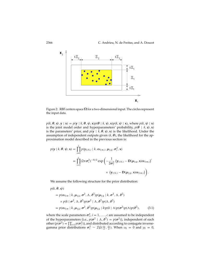
= p(α1:m | k,µ1:k,σ2, δ2)p(µ1:k | k)p(k | 3)p(σ2)p(3)p(δ2), (3.1)

where the scale parameters σ2i , i = 1, . . . , c are assumed to be independent

of the hyperparameters (i.e., p(σ2 | 3, δ2) = p(σ2)), independent of eachother (p(σ2) =∏c

i=1 p(σ2i )), and distributed according to conjugate inverse-

gamma prior distributions σ2i ∼ IG( υ0

2 ,γ02 ). When υ0 = 0 and γ0 = 0,


we obtain Jeffreys’s uninformative prior p(σ2i ) ∝ 1/σ2

i (Bernardo & Smith,1994). Given σ2, we introduce the following prior distribution:

p(k,α1:m,µ1:k | σ2,3, δ2) = p(α1:m | k,µ1:k,σ

2, δ2)p(µ1:k | k)p(k | 3)

=[

c∏i=1

|2πσ2i Σi|−1/2exp

(− 1

2σ2iα′1:m,iΣ

−1i α1:m,i

)]

×[ IΩ(k,µ1:k)

=k

] 3k/k!∑kmaxj=0 3

j/j!

,where Σ−1

i = δ−2i D′(µ1:k, x)D(µ1:k, x) and IΩ(k,µ1:k) is the indicator func-

tion of the set Ω (1 if (k,µ1:k) ∈ Ω, 0 otherwise).The prior model order distribution p(k | 3) is a truncated Poisson distri-

bution. Conditional on k, the RBF centers are uniformly distributed. Finally,conditional on (k,µ1:k), the coefficients α1:m,i are assumed to be zero-meangaussian with variance σ2

i Σi. The terms δ2 ∈ (R+)c and 3 ∈ R+ can berespectively interpreted as the expected signal-to-noise ratios and the ex-pected number of radial basis. The prior for the coefficients has been previ-ously advocated by various authors (George & Foster, 1997; Smith & Kohn,1996). It corresponds to the popular g-prior distribution (Zellner, 1986) andcan be derived using a maximum entropy approach (Andrieu, 1998). Animportant property of this prior is that it penalizes for basis functions beingtoo close as, in this situation, the determinant of Σ−1

i tends to zero.We now turn our attention to the hyperparameters, which allow us to

accomplish our goal of designing robust model selection schemes. We as-sume that they are independent of each other, that is, p(3, δ2) = p(3)p(δ2).Moreover, p(δ2) =∏c

i=1 p(δ2i ). As δ2 is a scale parameter, we ascribe a vague

conjugate prior density to it: δ2i ∼ IG(αδ2 , βδ2) for i = 1, . . . , c, with αδ2 = 2

and βδ2 > 0. The variance of this hyperprior with αδ2 = 2 is infinite. Weapply the same method to 3 by setting an uninformative conjugate prior(Bernardo & Smith, 1994): 3 ∼ Ga(1/2 + ε1, ε2) (εi ¿ 1 i = 1, 2). We canvisualize our hierarchical prior (see equation 3.1) with a directed acyclicgraphical model (DAG), as shown in Figure 3.

3.2 Estimation and Inference Aims. The Bayesian inference of k, θ, andψ is based on the joint posterior distribution p(k,θ,ψ | x,y) obtained fromBayes’s theorem. Our aim is to estimate this joint distribution from which, bystandard probability marginalization and transformation techniques, onecan “theoretically” obtain all posterior features of interest. For instance, wemight wish to perform inference with the predictive density:

p(yN+1 | x1:N+1,y1:N)

=∫Θ×Ψ

p(yN+1 | k,θ,ψ, xN+1)p(k,θ,ψ | x1:N,y1:N)dk dθ dψ


ε2

ε1

βδ2αδ2 υ0γ

0 Λ

δ2

α µ

yx

kσ 2

Figure 3: Directed acyclic graphical model for our prior.

and consequently make predictions, such as:

E(yN+1 | x1:N+1,y1:N)

=∫Θ×Ψ

D(µ1:k, xN+1)α1:mp(k,θ,ψ | x1:N,y1:N)dk dθ dψ.

We might also be interested in evaluating the posterior model probabilitiesp(k | x,y), which can be used to perform model selection by selecting themodel order as arg maxk∈0,...,kmax p(k | x,y). In addition, it allows us toperform parameter estimation by computing, for example, the conditionalexpectation E(θ | k, x,y).

However, it is not possible to obtain these quantities analytically, as it re-quires the evaluation of high-dimensional integrals of nonlinear functionsin the parameters, as we shall see in the following section. We propose hereto use an MCMC method to perform Bayesian computation. MCMC tech-niques were introduced in the mid-1950s in statistical physics and startedappearing in the fields of applied statistics, signal processing, and neuralnetworks in the 1980s and 1990s (Holmes & Mallick, 1998; Neal, 1996; RiosInsua & Muller, 1998; Robert & Casella, 1999; Tierney, 1994). The key ideais to build an ergodic Markov chain (k(i),θ(i),ψ(i))i∈N whose equilibriumdistribution is the desired posterior distribution. Under weak additionalassumptions, the PÀ 1 samples generated by the Markov chain are asymp-totically distributed according to the posterior distribution and thus allow


easy evaluation of all posterior features of interest—for example:

p(k = j | x,y) = 1P

P∑i=1

Ij(k(i))

and

E(θ | k = j, x,y) =∑P

i=1 θ(i)Ij(k(i))∑P

i=1 Ij(k(i)). (3.2)

In addition, we can obtain predictions, such as:

E(yN+1 | x1:N+1,y1:N) = 1P

P∑i=1

D(µ(i)1:k, xN+1)α(i)1:m.

3.3 Integration of the Nuisance Parameters. The proposed Bayesianmodel allows for the integration of the so-called nuisance parameters,α1:m

and σ2, and subsequently to obtain an expression for p(k,µ1:k,3, δ2 | x,y)

up to a normalizing constant. By applying Bayes’s theorem, multiplying theexponential terms of the likelihood and coefficients prior, and completingsquares, we obtain the following expression for the full posterior distribu-tion:

p(k,α1:m,µ1:k,σ2,3, δ2 | x,y)

∝[

c∏i=1

(2πσ2i )−N/2 exp

(− 1

2σ2i

y′1:N,iPi,ky1:N,i

)]

×[

c∏i=1

|2πσ2i Σi|−1/2

× exp(− 1

2σ2i

(α1:m,i − hi,k

)′M−1i,k

(α1:m,i − hi,k

))]

×[ IΩ(k,µ1:k)

=k

] 3k/k!∑kmaxj=0 3

j/j!

[ c∏i=1

(σ2i )−(υ0/2+1) exp

(− γ0

2σ2i

)]

×[

c∏i=1

(δ2i )−(α

δ2+1) exp

(−βδ2

δ2i

)][(3)(ε1−1/2) exp (−ε23)

],

where

M−1i,k = D′(µ1:k, x)D(µ1:k, x)+Σ−1

i , hi,k =Mi,kD′(µ1:k, x)y1:N,i

Pi,k = IN −D(µ1:k, x)Mi,kD′(µ1:k, x).


We can now integrate with respect to α1:m (gaussian distribution) and σ2i

(inverse gamma distribution) to obtain the following expression for theposterior:

p(k,µ1:k,3, δ2 | x,y)∝

c∏i=1

(1+ δ2

i

)−m/2(γ0 + y′1:N,iPi,ky1:N,i

2

)(− N+υ02

)×[ IΩ(k,µk)

=k

] 3k/k!∑kmaxj=0 3

j/j!

[ c∏i=1

(δ2i )−(α

δ2+1) exp

(−βδ

2

δ2i

)]

×[(3)(ε1−1/2) exp (−ε23)

]. (3.3)

It is worth noticing that the posterior distribution is highly nonlinear in theRBF centers µk and that an expression of p(k | x,y) cannot be obtained inclosed form.

4 Bayesian Computation

For clarity, we assume that k is given. After dealing with this fixed-dimensionscenario, we present an algorithm where k is treated as an unknown randomvariable.

4.1 MCMC Sampler for Fixed Dimension. We propose the followinghybrid MCMC sampler, which combines Gibbs steps and Metropolis-Hast-ings (MH) steps (Gilks, Richardson, & Spiegelhalter, 1996; Tierney, 1994):

Fixed-Dimension MCMC Algorithm

1. Initialization. Fix the value of k and set (θ(0), ψ(0)) and i = 1.

2. Iteration i

• For j = 1, . . . , k

— Sample u ∼ U[0,1].

— If u < $ , perform an MH step admitting p(µj,1:d | x,y, µ(i)−j,1:d)

as invariant distribution and q1(µ?j,1:d | µ(i)j,1:d) as proposal

distribution.

— Else perform an MH step using p(µj,1:d | x,y, µ(i)−j,1:d) as

invariant distribution and q2(µ?j,1:d | µ(i)j,1:d) as proposal dis-

tribution.

End For.

• Sample the nuisance parameters (α(i)1:m, σ2(i)) using equations 4.1

and 4.2.


• Sample the hyperparameters (3(i), δ2(i)) using equations 4.3 and4.4.

3. i← i+ 1 and go to 2.

The simulation parameter $ is a real number satisfying 0 < $ < 1. Itsvalue indicates our belief on which proposal distribution leads to fasterconvergence. If we have no preference for a particular proposal, we can setit to 0.5. The various steps of the algorithm are detailed in the followingsections. In order to simplify the notation, we drop the superscript ·(i) fromall variables at iteration i.

4.1.1 Updating the RBF Centers. Sampling the RBF centers is difficultbecause the distribution is nonlinear in these parameters. We have chosenhere to sample them one at a time using a mixture of MH steps. An MH stepof invariant distribution, say π(z), and proposal distribution, say q(z? | z),involves sampling a candidate value z? given the current value z accord-ing to q(z? | z). The Markov chain then moves toward z? with probabilityA(z, z?) , min1, (π(z)q(z? | z))−1π(z?) q(z | z?); otherwise, it remainsequal to z. This algorithm is very general, but to perform well in practice,it is necessary to use “clever” proposal distributions to avoid rejecting toomany candidates.

According to equation 3.3, the target distribution is the full conditionaldistribution of a basis center:

p(µj,1:d | x,y,µ−j,1:d)

∝

c∏i=1

(γ0 + y′1:N,iPi,ky1:N,i

2

)(− N+υ02

) IΩ(k,µ1:k),

where µ−j,1:d denotes µ1,1:d,µ2,1:d, . . . ,µj−1,1:d,µj+1,1:d, . . . ,µk,1:d.With probability 0 < $ < 1, the proposal q1(µ?j,1:d | µj,1:d) corresponds

to randomly sampling a basis center from the interval [min(x1:N,i) − ι4i,max(x1:N,i)+ ι4i]k for i = 1, . . . , d. The motivation for using such a proposaldistribution is that the regions where the data are dense are reached quickly.Subsequently, with probability 1−$ , we perform an MH step with proposaldistribution q2(µ?j,1:d | µj,1:d):

µ?j,1:d | µj,1:d ∼ N (µj,1:d, σ2RWId).

This proposal distribution yields a candidate µ?j,1:d, which is a perturbationof the current center. The perturbation is a zero-mean gaussian randomvariable with variance σ 2

RWId. This random walk is introduced to perform a


local exploration of the posterior distribution. In both cases, the acceptanceprobability is given by:

A(µj,1:d,µ?j,1:d)

= min

1,

c∏i=1


γ0 + y′1:N,iP?i,ky1:N,i

)( N+υ02

) IΩ(k,µ?1:k)

,where P?i,k and M?

i,k are similar to Pi,k and Mi,k with µ1:k,1:d replaced byµ1,1:d,µ2,1:d, . . ., µj−1,1:d,µ

?j,1:d,µj+1,1:d, . . . ,µk,1:d. We have found that the

combination of these proposal distributions works well in practice.

4.1.2 Sampling the Nuisance Parameters. In section 3.3, we derived anexpression for p(k,µ1:k,3, δ

2 | x,y) from the full posterior distributionp(k,α1:m, µ1:k, σ2, 3, δ2 | x,y) by performing some algebraic manipula-tions and integrating with respect to α1:m (gaussian distribution) and σ2

(inverse gamma distribution). As a result, if we take into consideration that

p(k,α1:m,µ1:k,σ2,3, δ2 | x,y)

= p(α1:m | k,µ1:k,σ2,3, δ2

, x,y)p(k,µ1:k,σ2,3, δ2 | x,y)

= p(α1:m | k,µ1:k,σ2,3, δ2, x,y)p(σ2 | k,µ1:k,3, δ

2, x,y)

× p(k,µ1:k,3, δ2 | x,y),

it follows that for i = 1, . . . , c, α1:m,i, and σ2i are distributed according to:

σ2i | (k,µ1:k, δ

2, x,y) ∼ IG

(υ0 +N

2,γ0 + y′1:N,iPi,ky1:N,i

2

)(4.1)

α1:m,i | (k,µ1:k,σ2, δ2, x,y) ∼ N (hi,k,σ

2i Mi,k). (4.2)

4.1.3 Sampling the Hyperparameters. By considering p(k,α1:m, µ1:k, σ2,3, δ2 | x,y), we can clearly see that the hyperparameters δi (for i = 1, . . . , c)can be simulated from the full conditional distribution:

δ2i | (k,α1:m,µ1:k,σ

2i , x,y)

∼ IG(αδ2 + m

2, βδ2 + 1

2σ2iα′1:m,iD

′(µ1:k, x)D(µ1:k, x)α1:m,i

). (4.3)

On the other hand, an expression for the posterior distribution of3 is not sostraightforward because the prior for k is a truncated Poisson distribution.3can be simulated using the MH algorithm with a proposal corresponding tothe full conditional that would be obtained if the prior for k was an infinite


Poisson distribution. That is, we can use the following gamma proposalfor 3,

q(3?) ∝ 3?(1/2+ε1+k) exp(−(1+ ε2)3

?), (4.4)

and subsequently perform an MH step with the full conditional distributionp(3 | k,µ1:k, δ

2, x,y) as invariant distribution.

4.2 MCMC Sampler for Unknown Dimension. Now let us consider thecase where k is unknown. Here, the Bayesian computation for the estimationof the joint posterior distribution p(k,θ,ψ | x,y) is even more complex.One obvious solution would consist of upper bounding k by, say, kmax andrunning kmax + 1 independent MCMC samplers, each being associated to afixed number k = 0, . . . , kmax. However, this approach suffers from severedrawbacks. First, it is computationally very expensive since kmax can belarge. Second, the same computational effort is attributed to each valueof k. In fact, some of these values are of no interest in practice becausethey have a very weak posterior model probability p(k | x,y). Anothersolution would be to construct an MCMC sampler that would be able tosample directly from the joint distribution on Θ ×Ψ = (∪kmax

k=0 k ×Θk) ×Ψ. Standard MCMC methods are not able to “jump” between subspacesΘk of different dimensions. However, Green (1995) has introduced a new,flexible class of MCMC samplers, the so-called reversible-jump MCMC,that are capable of jumping between subspaces of different dimensions.This is a general state-space MH algorithm (see Andrieu, Djuric, & Doucet,in press, for an introduction). One proposes candidates according to a set ofproposal distributions. These candidates are randomly accepted accordingto an acceptance ratio, which ensures reversibility and thus invariance of theMarkov chain with respect to the posterior distribution. Here, the chain mustmove across subspaces of different dimensions, and therefore the proposaldistributions are more complex (see Green, 1995 and Richardson & Green,1997, for details). For our problem, the following moves have been selected:

1. Birth of a new basis, that is, proposing a new basis function in theinterval [min(x1:N,i)− ι4i,max(x1:N,i)+ ι4i]k for i = 1, . . . , d.

2. Death of an existing basis, that is, removing a basis function chosenrandomly.

3. Merge a randomly chosen basis function and its closest neighbor intoa single basis function.

4. Split a randomly chosen basis function into two neighbor basis func-tions, such that the distance between them is shorter than the distancebetween the proposed basis function and any other existing basis func-tion. This distance constraint ensures reversibility.

5. Update the RBF centers.


These moves are defined by heuristic considerations, the only conditionto be fulfilled being to maintain the correct invariant distribution. A particu-lar choice will have influence only on the convergence rate of the algorithm.The birth and death moves allow the network to grow from k to k + 1 anddecrease from k to k − 1, respectively. The split and merge moves also per-form dimension changes from k to k + 1 and k to k − 1. The merge moveserves to avoid the problem of placing too many basis functions in the sameneighborhood. That is, when amplitudes of many basis functions, in a closeneighborhood, add to the amplitude that would be obtained by using fewerbasis functions, the merge move combines some of these basis functions. Onthe other hand, the split move is useful in regions of the data where there areclose components. Other moves may be proposed, but we have found thatthe ones suggested here lead to satisfactory results. In particular, we startedwith the update, birth, and death moves and noticed that by incorporatingsplit and merge moves, the estimation results improved.

The resulting transition kernel of the simulated Markov chain is thena mixture of the different transition kernels associated with the movesdescribed above. This means that at each iteration, one of the candidatemoves—birth, death, merge, split, or update—is randomly chosen. Theprobabilities for choosing these moves are bk, dk, mk, sk, and uk, respec-tively, such that bk + dk + mk + sk + uk = 1 for all 0 ≤ k ≤ kmax. A move isperformed if the algorithm accepts it. For k = 0 the death, split, and mergemoves are impossible, so that d0 , 0, s0 , 0, and m0 , 0. The merge moveis also not permitted for k = 1, that is, m1 , 0. For k = kmax, the birth andsplit moves are not allowed, and therefore bkmax , 0 and skmax , 0. Except inthe cases described above, we adopt the following probabilities:

bk , c? min

1,

p(k+ 1 | 3)p(k | 3)

,

dk+1 , c? min

1,

p(k | 3)

p(k+ 1 | 3)

, (4.5)

where p(k | 3) is the prior probability of modelMk and c? is a parameterthat tunes the proportion of dimension and update moves. As Green (1995)pointed out, this choice ensures that bkp(k | 3)[dk+1p(k+1 | 3)]−1 = 1, whichmeans that an MH algorithm in a single dimension, with no observations,would have 1 as acceptance probability. We take c? = 0.25 and then bk+dk+mk+ sk ∈ [0.25, 1] for all k (Green, 1995). In addition, we choose mk = dk andsk = bk. We can now describe the main steps of the algorithm as follows:

Reversible-Jump MCMC Algorithm

1. Initialization: set (k(0), θ (0), ψ(0)) ∈Θ×Ψ.


2. Iteration i.

• Sample u ∼ U[0,1].

• If (u ≤ bk(i) )

— then birth move (see section 4.2.1).

— else if (u ≤ bk(i)+dk(i) ) then death move (see section 4.2.1).

— else if (u ≤ bk(i) + dk(i) + sk(i) ) then split move (see section4.2.2).

— else if (u ≤ bk(i) + dk(i) + sk(i) + mk(i) ) then merge move(see section 4.2.2).

— else update the RBF centers (see section 4.2.3).

End If.

• Sample the nuisance parameters (σ 2(i)k , α

(i)k ) using equations 4.1

and 4.2.

• Simulate the hyperparameters (3(i), δ2(i)) using equations 4.3 and4.4.

3. i← i+ 1 and go to 2.

We expand on these different moves in the following sections. Once again,in order to simplify the notation, we drop the superscript ·(i) from all vari-ables at iteration i.

4.2.1 Birth and Death Moves. Suppose that the current state of the Markovchain is in k ×Θk ×Ψ. Then the algorithm for the birth and death movesis as follows:

Birth Move

1. Propose a new basis location at random from the interval [min(x1:N,i)−ι4i,

max(x1:N,i)+ ι4i] for i = 1, . . . , d.

2. Evaluate Abirth (see equation 4.7), and sample u ∼ U[0,1].

3. If u ≤ Abirth, then the state of the Markov chain becomes (k + 1, µ1:k+1),else it remains equal to (k, µ1:k).

Death move

1. Choose the basis center to be deleted, at random among the k existingbasis.

2. Evaluate Adeath (see equation 4.7), and sample u ∼ U[0,1].

3. If u ≤ Adeath then the state of the Markov chain becomes (k − 1, µ1:k−1),else it remains equal to (k, µ1:k).


The acceptance ratio for the proposed birth move is deduced from thefollowing expression (Green, 1995):

rbirth , (posterior distributions ratio)× (proposal ratio)× (Jacobian)

= p(k+ 1,µ1:k+1,3, δ2 | x,y)

p(k,µ1:k,3, δ2|x,y)

× dk+1/(k+ 1)bk/=

×∣∣∣∣ ∂(µ1:k+1)

∂(µ1:k,µ?)

∣∣∣∣ .Clearly, the Jacobian is equal to 1, and after simplifications we obtain:

rbirth =

c∏i=1

1

(1+ δ2i )

1/2


γ0 + y′1:N,iPi,k+1y1:N,i

)( N+υ02

) 1(k+ 1)

.

Similarly, for the death move:

rdeath =p(k− 1,µ1:k−1,3, δ

2|x,y)

p(k,µ1:k,3, δ2|x,y)

× bk−1/=dk/k

×∣∣∣∣∂(µ1:k−1,µ

?)

∂(µ1:k)

∣∣∣∣=

c∏i=1

(1+ δ2i )

1/2


γ0 + y′1:N,iPi,k−1y1:N,i

)( N+υ02

) k. (4.6)

The acceptance probabilities corresponding to the described moves are:

Abirth = min 1, rbirth , Adeath = min 1, rdeath (4.7)

4.2.2 Split and Merge Moves. The merge move involves randomly se-lecting a basis function (µ1) and then combining it with its closest neighbor(µ2) into a single basis function µ, whose new location is

µ = µ1 +µ2

2. (4.8)

The corresponding split move that guarantees reversibility is

µ1 = µ− umsς?

µ2 = µ+ umsς?, (4.9)

where ς? is a simulation parameter and ums ∼ U[0,1]. To ensure reversibility,we perform the merge move only if ‖µ1−µ2‖ < 2ς?. Suppose now that thecurrent state of the Markov chain is in k×Θk×Ψ. Then the algorithm forthe split and merge moves is as follows:

Split Move1. Randomly choose an existing RBF center.


2. Substitute it for two neighbor basis functions, whose centers are obtainedusing equation 4.9. The new centers must be bound to lie in the space Ωk,and the distance (typically Euclidean) between them has to be shorter thanthe distance between the proposed basis function and any other existingbasis function.

3. Evaluate Asplit (see equation 4.10), and sample u ∼ U[0,1].

4. If u ≤ Asplit then the state of the Markov chain becomes (k + 1, µ1:k+1),else it remains equal to (k, µ1:k).

Merge Move

1. Choose a basis center at random among the k existing basis. Then findthe closest basis function to it applying some distance metric, for example,Euclidean.

2. If ‖µ1 − µ2‖ < 2ς?, substitute the two basis functions for a single basisfunction in accordance with equation 4.8.

3. Evaluate Amerge (see equation 4.10), and sample u ∼ U[0,1].

4. If u ≤ Amerge, then the state of the Markov chain becomes (k − 1, µ1:k−1),else it remains equal to (k, µ1:k).

The acceptance ratio for the proposed split move is given by:

rsplit =p(k+ 1,µ1:k+1,3, δ

2|x,y)

p(k,µ1:k, k,3, δ2|x,y)× mk+1/(k+ 1)

p(ums)sk/k×∣∣∣∣∂(µ1,µ2)

∂(µ,ums)

∣∣∣∣ .In this case, the Jacobian is equal to:

Jsplit =∣∣∣∣∂(µ1,µ2)

∂(µ,ums)

∣∣∣∣ = ∣∣∣∣ 1 1−ς? ς?

∣∣∣∣ = 2ς?,

and, after simplifications, we obtain:

rsplit =

c∏i=1

1

(1+ δ2i )

1/2


γ0 + y′1:N,iPi,k+1y1:N,i

)( N+υ02

) kς?

=(k+ 1).

Similarly, for the merge move:

rmerge = p(k− 1,µ1:k−1,3, δ2|x,y)

p(k,µ1:k,3, δ2|x,y)

× sk−1/(k− 1)mk/k

×∣∣∣∣ ∂(µ,ums)

∂(µ1,µ2)

∣∣∣∣ ,


and, since Jmerge = 1/2ς?, it follows that

rmerge =

c∏i=1

(1+ δ2i )

1/2


γ0 + y′1:N,iPi,k−1y1:N,i

)( N+υ02

) k=ς?(k− 1)

.

The acceptance probabilities for the split and merge moves are:

Asplit = min1, rsplit

, Amerge = min

1, rmerge

. (4.10)

4.2.3 Update Move. The update move does not involve changing the di-mension of the model. It requires an iteration of the fixed dimension MCMCsampler presented in section 4.1.1.

The method presented so far can be very accurate, yet it can be compu-tationally demanding. In the following section, we present a method thatrequires optimization instead of integration to obtain estimates of the pa-rameters and model dimension. This method, although less accurate, asshown in section 7, is less computationally demanding. The choice of onemethod over the other should ultimately depend on the modeling con-straints and specifications.

5 Reversible-Jump Simulated Annealing

In this section, we show that traditional model selection criteria within apenalized likelihood framework, such as AIC, BIC, and MDL (Akaike, 1974;Schwarz, 1985; Rissanen, 1987), can be shown to correspond to particular hy-perparameter choices in our hierarchical Bayesian formulation. (As pointedout by one of the reviewers, AIC is not restricted to the situation where thetrue model belongs to the set of model candidates.) That is, we can calibratethe prior choices so that the problem of model selection within the penalizedlikelihood context can be mapped exactly to a problem of model selectionvia posterior probabilities. This technique has been previously applied tothe problem of variable selection (George & Foster, 1997).

After resolving the calibration problem, we perform maximum like-lihood estimation, with the model selection criteria, by maximizing thecalibrated posterior distribution. To accomplish this goal, we adopt anMCMC simulated annealing algorithm, which makes use of the homo-geneous reversible-jump MCMC kernel as proposal distribution. This ap-proach has the advantage that we can start with an arbitrary model order,and the algorithm will perform dimension jumps until it finds the “true”model order. That is, we do not have to resort to the more expensive taskof running a fixed-dimension algorithm for each possible model order andsubsequently select the best model.


5.1 Penalized Likelihood Model Selection. Traditionally, penalized like-lihood model order selection strategies, based on standard information cri-teria, require the evaluation of the maximum likelihood (ML) estimates foreach model order. The number of required evaluations can be prohibitivelyexpensive unless appropriate heuristics are available. Subsequently, a par-ticular modelMs is selected if it is the one that minimizes the sum of thethe log-likelihood and a penalty term that depends on the model dimension(Djuric, 1998; Gelfand & Dey, 1997). In mathematical terms, this estimate isgiven by:

Ms = arg minMk: k∈0,...,kmax

− log(p(y | k, θ, x))+ P

, (5.1)

where θ = (α1:m, µ1:k, σ2k) is the ML estimate of θ for model Mk. P is a

penalty term that depends on the model order. Examples of ML penaltiesinclude the well-known AIC, BIC, or MDL information criteria (Akaike,1974; Schwarz, 1985; Rissanen, 1987). The expressions for these in the caseof gaussian observation noise are

PAIC = ξ and PBIC = PMDL = ξ

2log(N),

where ξ denotes the number of model parameters (k(c+1)+ c(1+d)) in thecase of an RBF network). These criteria are motivated by different factors:AIC is based on expected information, BIC is an asymptotic Bayes factor, andMDL involves evaluating the minimum information required to transmitsome data and a model, which describes the data, over a communicationschannel.

Using the conventional estimate of the variance for gaussian distribu-tions,

σ2i =

1N


)′ (y1:N,i −D(µ1:k, x)α1:m,i)

= 1N

y′1:N,iP∗i,ky1:N,i,

where P∗i,k is the least-squares orthogonal projection matrix,

P∗i,k = IN −D(µ1:k, x)[D′(µ1:k, x)D(µ1:k, x)

]−1 D′(µ1:k, x),

we can expand equation 5.1 as follows:

Ms = arg minMk:k∈0,...,kmax

− log

[c∏

i=1

(2πσ2i )−N/2


× exp

(− 1

2σ2i


)′× (

y1:N,i −D(µ1:k, x)α1:m,i) )]+ P

= arg maxMk :k∈0,...,kmax

[c∏

i=1

(y′1:N,iP∗i,ky1:N,i)

−N/2

]exp(−P)

. (5.2)

In the following section, we show that calibrating the priors in our hierar-chical Bayes model will lead to the expression given by equation 5.2.

5.2 Calibration. It is useful and elucidating to impose some restrictionson the Bayesian hierarchical prior (see equation 3.3) to obtain the AIC andMDL criteria. We begin by assuming that the hyperparameter δ is fixed toa particular value, say δ, and that we no longer have a definite expressionfor the model prior p(k), so that

p(k,µ1:k | x,y)

∝

c∏i=1

(1+ δ2i )−m/2


2

)(− N+υ02

)[ IΩ(k,µk)

=k

]p(k).

Furthermore, we set υ0 = 0 and γ0 = 0 to obtain Jeffreys’s uninformativeprior p(σ2

i ) ∝ 1/σ2i . Consequently, we obtain the following expression:

p(k,µ1:k | x,y)

∝[

c∏i=1

(1+ δ2

i

)−k/2 (y′1:N,iPi,ky1:N,i

)− N2

][ IΩ(k,µk)

=k

]p(k),

where M−1i,k = (1+δ

−2i )D′(µ1:k, x)D(µ1:k, x), hi,k =Mi,kD′(µ1:k, x)y1:N,i, and

Pi,k = IN −D(µ1:k, x)Mi,kD′(µ1:k, x). Finally, we can select δ2i and p(k) such

that [c∏

i=1

(1+ δ2

i

)−k/2][ IΩ(k,µk)

=k

]p(k) = exp(−P) ∝ exp(−Ck),

thereby ensuring that the expression for the calibrated posterior distribu-tion p(k,µ1:k | x,y) corresponds to the term that needs to be maximizedin the penalized likelihood framework (see equation 5.2). Note that for thepurposes of optimization, we only need the proportionality condition withC = c + 1 for the AIC criterion and C = (c + 1) log(N)/2 for the MDL and


BIC criteria. We could, for example, satisfy the proportionality by remain-ing in the compact set Ω and choosing the prior p(k) = 3k∑kmax

j=03j

, with the

following fixed value for 3:

3 =[

c∏i=1

(1+ δ2

i

) 12

]= exp (−C) . (5.3)

In addition, we have to let δ→∞ so that Pi,k → P∗i,k.We have thus shown that by calibrating the priors in the hierarchical

Bayesian formulation, in particular by treating3 and δ2 as fixed quantitiesinstead of as random variables, letting δ → ∞, choosing an uninforma-tive Jeffreys’s prior for σ2 and setting 3 as in equation 5.3, we can obtainthe expression that needs to be maximized in the classical penalized likeli-hood formulation with AIC, MDL, and BIC model selection criteria. Conse-quently, we can interpret the penalized likelihood framework as a problemof maximizing the joint posterior distribution p(k,µ1:k | x,y). Effectively,we can obtain this MAP estimate as follows:

(k,µ1:k)MAP = arg maxk,µ1:k∈Ω

p(k,µ1:k | x,y)

= arg maxk,µ1:k∈Ω

[c∏

i=1


−N/2

]exp(−P)

.

The sufficient conditions that need to be satisfied so that the distributionp(k,µ1:k | x,y) is proper are not overly restrictive. First, Ω has to be acompact set, which is not a problem in our setting. Second, y′1:N,iP

∗i,ky1:N,i

has to be larger than zero for i = 1, . . . , c. In appendix B, lemma 1, we showthat this is the case unless y1:N,i spans the space of the columns of D(µ1:k, x),in which case y′1:N,iP

∗i,ky1:N,i = 0. This event has probability zero.

5.3 Reversible-Jump Simulated Annealing. From an MCMC perspec-tive, we can solve the stochastic optimization problem posed in the previoussection by adopting a simulated annealing strategy (Geman & Geman, 1984;Van Laarhoven & Arts, 1987). The simulated annealing method involvessimulating a nonhomogeneous Markov chain whose invariant distributionat iteration i is no longer equal to π(z), but to πi(z) ∝ π1/Ti(z), where Ti is adecreasing cooling schedule with limi→+∞ Ti = 0. The reason for doing thisis that under weak regularity assumptions on π(z), π∞(z) is a probabilitydensity that concentrates itself on the set of global maxima of π(z).

As with the MH method, the simulated annealing method with distribu-tion π(z) and proposal distribution q(z? | z) involves sampling a candidatevalue z? given the current value z according to q(z? | z). The Markov chain


moves toward the candidate z? with probabilityASA (z, z?)= min1, (π1/Ti

(z)q(z? | z))−1π1/Ti(z?)q(z | z?); otherwise, it remains equal to z. If wechoose the homogeneous transition kernel K(z, z?) of the reversible-jumpalgorithm as the proposal distribution and use the reversibility property,

π(z?)K(z?, z) = π(z)K(z, z?),

it follows that

ARJSA = min

1,π(1/Ti−1)(z?)π(1/Ti−1)(z)

. (5.4)

Consequently, the following algorithm, with bk = dk = mk = sk = uk = 0.2,can find the joint MAP estimate of µ1:k and k:

Reversible-Jump Simulated Annealing

1. Initialization: set (k(0), θ (0)) ∈Θ.

2. Iteration i.

• Sample u ∼ U[0,1], and set the temperature according to the coolingschedule.

• If (u ≤ bk(i) )

— then birth move (see equation 5.6).

— else if (u ≤ bk(i)+dk(i) ) then death move (see equation 5.6).

— else if (u ≤ bk(i) + dk(i) + sk(i) ) then split move (see equa-tion 5.7).

— else if (u ≤ bk(i) + dk(i) + sk(i) +mk(i) ) then merge move (seeequation 5.7).

— else update the RBF centers (see equation 5.5).

End If.

• Perform an MH step with the annealed acceptance ratio (see equa-tion 5.4).

3. i← i+ 1 and go to 2.

4. Compute the coefficients α1:m by least squares (optimal in this case):

α1:m,i = [D′(µ1:k, x)D(µ1:k, x)]−1D′(µ1:k, x)y1:N,i.

We explain the simulated annealing moves in the following sections.To simplify the notation, we drop the superscript ·(i) from all variables atiteration i.


5.4 Moves. We sample the radial basis centers in the same way as ex-plained in section 4.1.1. However, the target distribution is given by

p(µj,1:d | x,y,µ−j,1:d) ∝[

c∏i=1


(− N

2

)]exp(−P),

and, consequently, the acceptance probability is

Aupdate(µj,1:d,µ?j,1:d) = min

1,

c∏i=1

(y′1:N,iP

∗i,ky1:N,i

y′1:N,iP?i,ky1:N,i

)( N2

) , (5.5)

where P?i,k is similar to P∗i,k withµ1:k,1:d replaced by µ1,1:d,µ2,1:d, . . . ,µj−1,1:d,

µ?j,1:d,µj+1,1:d, . . . ,µk,1:d. The birth and death moves are similar to the onesproposed in section 4.2.1, except that the expressions for rbirth and rdeath (withbk = dk = 0.2) become

rbirth =

c∏i=1

(y′1:N,iP

∗i,ky1:N,i

y′1:N,iP∗i,k+1y1:N,i

)( N2

) = exp(−C)k+ 1

.

Similarly,

rdeath =

c∏i=1

(y′1:N,iP

∗i,ky1:N,i

y′1:N,iP∗i,k−1y1:N,i

)( N2

) k exp(C)= .

Hence, the acceptance probabilities corresponding to the described movesare

Abirth = min 1, rbirth , Adeath = min 1, rdeath . (5.6)

Similarly, the split and merge moves are analogous to the ones proposedin section 4.2.2, except that the expressions for rsplit and rmerge (with mk =sk = 0.2) become

rsplit =

c∏i=1

(y′1:N,iP

∗i,ky1:N,i

y′1:N,iP∗i,k+1y1:N,i

)( N2

) kς? exp(−C)k+ 1


and

rmerge =

c∏i=1

(y′1:N,iP

∗i,ky1:N,i

y′1:N,iP∗i,k−1y1:N,i

)( N2

) k exp(C)ς?(k− 1)

.

The acceptance probabilities for these moves are

Asplit = min1, rsplit

, Amerge = min

1, rmerge

. (5.7)

6 Convergence Results

It is easy to prove that the reversible-jump MCMC algorithm applied tothe full Bayesian model converges, in other words, that the Markov chain(k(i),µ(i)1:k,3

(i), δ2(i))i∈N is ergodic. We prove here a stronger result by show-ing that (k(i),µ(i)1:k,3

(i), δ2(i))i∈N converges to the required posterior distribu-

tion at a geometric rate. For the homogeneous kernel, we have the followingresult:

Theorem 1. Let (k(i),µ(i)1:k,3(i), δ2(i))i∈N be the Markov chain whose transition

kernel has been described in section 3. This Markov chain converges to the prob-ability distribution p(k,µ1:k,3, δ

2 | x,y). Furthermore, this convergence occursat a geometric rate, that is, for p(k,µ1:k,3, δ

2 | x,y)-almost every initial point(k(0),µ(0)1:k,3

(0), δ2(0)) ∈ Ω×Ψ there exists a function C(k(0),µ(0)1:k,3

(0), δ2(0)) >

0 and a constant ρ ∈ [0, 1) such that:∥∥∥p(i)(

k,µ1:k,3, δ2)− p

(k,µ1:k,3, δ

2∣∣∣ x,y

)∥∥∥TV

≤ C(

k(0),µ(0)1:k,3(0), δ2(0)

)ρbi/kmaxc (6.1)

where p(i)(k,µ1:k,3, δ2) is the distribution of (k(i),µ(i)1:k,3

(i), δ2(i)) and ‖ · ‖TV isthe total variation norm (Tierney, 1994).

Proof. See appendix B.

Corollary 1. Since at each iteration i, one simulates the nuisance parameters(α1:m,σ2

k), the distribution of the series (k(i),α(i)1:m,µ(i)1:k,σ

2(i)k ,3(i), δ2(i)

)i∈N con-verges geometrically toward p(k,α1:m,µ1:k,σ

2k,3, δ

2 | x,y) at the same rate ρ.

In other words, the distribution of the Markov chain converges at least ata geometric rate, dependent on the initial state, to the required equilibriumdistribution p(k,θ, ψ | x,y).


Remark 1. In practice one cannot evaluate ρ, but theorem 1 proves itsexistence. This type of convergence ensures that a central limit theorem forergodic averages is valid (Meyn & Tweedie, 1993; Tierney, 1994). Moreover,in practice, there is empirical evidence that the Markov chain convergesquickly.

We have the following convergence theorem for the reversible-jumpMCMC simulated annealing algorithm:

Theorem 2. Under certain assumptions found in Andrieu, Breyer, and Doucet(1999), the series of (θ(i), k(i)) converges in probability to the set of global maxima(θmax

, kmax), that is, for any ε > 0, it follows that

limi→∞Pr

(p(θ(i), k(i))

p(θmax, kmax)≥ 1− ε

)= 1.

Proof. If we follow the same steps as in proposition 1 of appendix B,with δ2 and 3 fixed, it is easy to show that the transition kernels for eachtemperature are uniformly geometrically ergodic. Hence, as a corollary ofAndrieu et al. (1999, theorem 1), the convergence result for the simulatedannealing MCMC algorithm follows.

7 Experiments

When implementing the reversible-jump MCMC algorithm discussed insection 4, one might encounter problems of ill conditioning, in particularfor high-dimensional parameter spaces. There are two satisfactory waysof overcoming this problem.3 First, we can introduce a ridge regressioncomponent so that the expression for M−1

i,k in section 3.3 becomes

M−1i,k = D′(µ1:k, x)D(µ1:k, x)+Σ−1

i + ~Im,

where ~ is a small number. Alternatively, we can introduce a slight modifi-cation of the prior for α1:m:

p(α1:m | k,µ1:k,σ2,3, δ2

)

=[

c∏i=1

|2πσ2i δ

2i Im|−1/2 exp

(− 1

2σ2i δ

2i

α′1:m,iα1:m,i

)].

3 The software is available online at http://www.cs.berkeley.edu/∼jfgf.


We have found that although both strategies can deal with the problem oflimited numerical precision, the second approach seems to be more stable.In addition, the second approach does not oblige us to select a value for thesimulation parameter ~.

7.1 Experiment 1: Signal Detection. The problem of detecting signalcomponents in noisy signals has occupied the minds of many researchers fora long time (Djuric, 1996). Here, we consider the rather simple toy problem ofdetecting gaussian components in a noisy signal. Our aim is to compare theperformance of the hierarchical Bayesian model selection scheme and thepenalized likelihood model selection criteria (AIC, MDL) when the amountof noise in the signal varies.

The data were generated from the following univariate function using50 covariate points uniformly on [−2, 2]:

y = x+ 2 exp(−16x2)+ 2 exp(−16(x− 0.7)2)+ n,

where n ∼ N (0, σ 2). The data were then rescaled to make the input data liein the interval [0, 1]. We used the reversible-jump MCMC algorithm, for thefull Bayesian model, and the simulated annealing algorithms to estimate thenumber of components in the signal for different levels of noise. We repeatedthe experiment 100 times for each noise level. We chose gaussian radial basisfunctions with the same variance as the gaussian signal components. Forthe simulated annealing method, we adopted a linear cooling schedule:Ti = a − bi, where a, b ∈ R+ and Ti > 0 for i = 1, 2, 3, . . . In particular, weset the initial and final temperatures to 1 and 1 × 10−5. For the Bayesianmodel, we selected diffuse priors (αδ2 = 2, βδ2 = 10 [see experiment 2],υ0 = 0, γ0 = 0, ε1 = 0.001 and ε2 = 0.0001). Finally, we set the simulationparameters kmax, ι, σ 2

RW , and ς? to 20, 0.1, 0.001, and 0.1.Figure 4 shows the typical fits that were obtained for training and valida-

tion data sets. By varying the variance of the noise σ 2, we estimated the mainmode and fractions of unexplained variance. For the AIC and BIC/MDLcriteria, the main mode corresponds to the one for which the posterior ismaximized, while for the Bayesian approach, the main mode corresponds tothe MAP of the model order probabilities p(k | x,y), computed as suggestedin section 3.2.

The fractions of unexplained variance (fv) were computed as follows:

fv = 1100

100∑i=1

∑50t=1(yt,i − yt,i)

2∑50t=1(yt,i − yi)

2,

where yt,i denotes the tth prediction for the ith trial and yi is the estimatedmean of yi. The normalization in the fv error measure makes it independentof the size of the data set. If the estimated mean was to be used as the


0 0.1 0.2 0.3 0.4 0.5 0.6 0.7 0.8 0.9 1−4

−2

0

2

4

Tra

in o

utpu

t

Train input

0 0.1 0.2 0.3 0.4 0.5 0.6 0.7 0.8 0.9 1−6

−4

−2

0

2

4

Tes

t out

put

Test input

True functionTest data Prediction

Figure 4: Performance of the reversible-jump MCMC algorithm on the signaldetection problem. Despite the large noise variance, the estimates of the truefunction and noise process are very accurate, thereby leading to good generali-sation (no overfitting).

Table 1: Fraction of Unexplained Variance for Different Values of the NoiseVariance, Averaged over 100 Test Sets.

σ 2 AIC BIC/MDL Bayes

0.01 0.0070 0.0076 0.00690.1 0.0690 0.0732 0.06571 0.6083 0.4846 0.5105

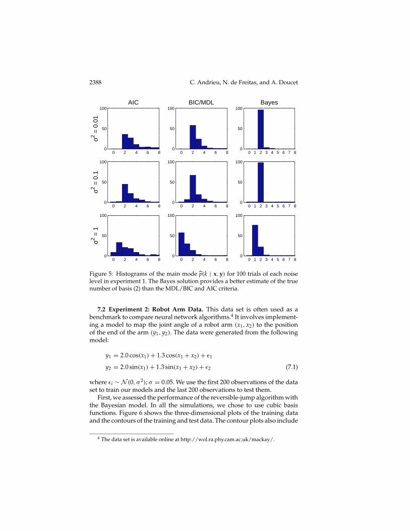
predictor of the data, the fv would be equal to 1. The results obtained areshown in Figure 5 and Table 1. The fv for each model selection approach arevery similar. This result is expected since the problem under considerationis rather simple and the error variations could possibly be attributed to thefact that we use only 100 realizations of the noise process for each σ 2. Whatis important is that even in this scenario, it is clear that the full Bayesianmodel provides more accurate estimates of the model order.


0 2 4 6 80

50

100

σ2 = 0

.01

AIC

0 2 4 6 80

50

100BIC/MDL

0 1 2 3 4 5 6 7 80

50

100Bayes

0 2 4 6 80

50

100

σ2 = 0

.1

0 2 4 6 80

50

100

0 1 2 3 4 5 6 7 80

50

100

0 2 4 6 80

50

100

σ2 = 1

0 2 4 6 80

50

100

0 1 2 3 4 5 6 7 80

50

100

Figure 5: Histograms of the main mode p(k | x,y) for 100 trials of each noiselevel in experiment 1. The Bayes solution provides a better estimate of the truenumber of basis (2) than the MDL/BIC and AIC criteria.

7.2 Experiment 2: Robot Arm Data. This data set is often used as abenchmark to compare neural network algorithms.4 It involves implement-ing a model to map the joint angle of a robot arm (x1, x2) to the positionof the end of the arm (y1, y2). The data were generated from the followingmodel:

y1 = 2.0 cos(x1)+ 1.3 cos(x1 + x2)+ ε1

y2 = 2.0 sin(x1)+ 1.3 sin(x1 + x2)+ ε2 (7.1)

where εi ∼ N (0, σ 2); σ = 0.05. We use the first 200 observations of the dataset to train our models and the last 200 observations to test them.

First, we assessed the performance of the reversible-jump algorithm withthe Bayesian model. In all the simulations, we chose to use cubic basisfunctions. Figure 6 shows the three-dimensional plots of the training dataand the contours of the training and test data. The contour plots also include

4 The data set is available online at http://wol.ra.phy.cam.ac.uk/mackay/.


−20

2

02

4−5

0

5

x1x2

y1

−2 −1 0 1 20

1

2

3

4

Tra

in s

et

−2 −1 0 1 20

1

2

3

4

Tes

t set

−20

2

02

4−5

0

5

x1x2

y2−2 −1 0 1 20

1

2

3

4

−2 −1 0 1 20

1

2

3

4

Figure 6: (Top) Training data surfaces corresponding to each coordinate of therobot arm’s position. (Middle, bottom) Training and validation data (solid lines)and respective RBF network mappings (dotted lines).

the typical approximations that were obtained using the algorithm. To assessconvergence, we plotted the probabilities of each model order p(k | x,y) inthe chain (using equation 3.2) for 50,000 iterations, as shown in Figure 7. Asthe model orders begin to stabilize after 30,000 iterations, we decided to runthe Markov chains for 50,000 iterations with a burn-in of 30,000 iterations. Itis possible to design more complex convergence diagnostic tools; however,this topic is beyond the scope of this article.

We chose uninformative priors for all the parameters and hyperparam-eters. In particular, we used the values shown in Table 2. To demonstratethe robustness of our model, we chose different values for βδ2 (the only crit-ical hyperparameter as it quantifies the mean of the spread δ of αk). Theobtained mean square errors (see Table 2) and probabilities for δ1, δ2, σ2

1,k,σ2

2,k, and k, shown in Figure 8, clearly indicate that our model is robust withrespect to prior specification.

As shown in Table 3, our mean square errors are slightly better than theones reported by other researchers (Holmes & Mallick, 1998; Mackay, 1992;Neal, 1996; Rios Insua & Muller, 1998). Yet the main point we are trying tomake is that our model exhibits the important quality of being robust to the


0 0.5 1 1.5 2 2.5 3 3.5 4 4.5 5

x 104

0

0.1

0.2

0.3

0.4

0.5

0.6

0.7

0.8

0.9

1

Iteration number

p(k|

x,y)

13141516

Figure 7: Convergence of the reversible-jump MCMC algorithm for RBF net-works. The plot shows the probability of each model order given the data. Themodel orders begin to stabilize after 30,000 iterations.

Table 2: Simulation Parameters and Mean Square Errors for the Robot ArmData (Test Set) Using the Reversible-Jump MCMC Algorithm and the BayesianModel.

αδ2 βδ2 υ0 γ0 ε1 ε2 Mean Square Error

2 0.1 0 0 0.0001 0.0001 0.005052 10 0 0 0.0001 0.0001 0.005032 100 0 0 0.0001 0.0001 0.00502

prior specification and statistically significant. Moreover, it leads to moreparsimonious models than the ones previously reported.

We also tested the reversible-jump simulated annealing algorithms withthe AIC and MDL criteria on this problem. The results for the MDL criterionare depicted in Figure 9. We note that the posterior increases stochasticallywith the number of iterations and eventually converges to a maximum. Thefigure also illustrates the convergence of the train and test set errors for each


0 100 2000

0.1

0.2

β δ2 =

0.1

δ12 and δ

22

0 2 4 6

x 10−3

0

0.02

0.04

0.06

σ12 and σ

22

12 14 160

0.2

0.4

0.6

0.8k

0 100 2000

0.1

0.2

β δ2 =

100

0 2 4 6

x 10−3

0

0.02

0.04

0.06

12 14 160

0.2

0.4

0.6

0.8

0 100 2000

0.1

0.2

β δ2 =

10

0 2 4 6

x 10−3

0

0.02

0.04

0.06

12 14 160

0.2

0.4

0.6

0.8

Figure 8: Histograms of smoothness constraints for each output (δ1 and δ2),noise variances (σ 2

1,k and σ 22,k), and model order (k) for the robot arm data sim-

ulation using three different values for βδ2 . The plots confirm that the model isrobust to the setting of βδ2 .

network in the Markov chain. For the final network, we chose the one thatmaximized the posterior (the MAP estimate). This network consisted of 12basis functions and incurred an error of 0.00512 in the test set. Followingthe same procedure, the AIC network consisted of 27 basis functions andincurred an error of 0.00520 in the test set. These results indicate that thefull Bayesian model, with model averaging, provides more accurate results.Moreover, it seems that the information criteria, in particular the AIC, canlead to overfitting of the data.

These results confirm the well-known fact that suboptimal techniques,such as the simulated annealing method with information criteria penaltyterms and a rapid cooling schedule, can allow for faster computation at theexpense of accuracy.


Table 3: Mean Square Errors and Number of Basis Functions for the Robot ArmData.

Method Mean Square Error

Mackay’s (1992) gaussian approximation with highest evidence 0.00573Mackay’s (1992) gaussian approximation with lowest test error 0.00557Neal’s (1996) hybrid Monte Carlo 0.00554Neal’s (1996) hybrid Monte Carlo with ARD 0.00549Rios Insua and Muller’s (1998) MLP with reversible-jump MCMC 0.00620Holmes and Mallick’s (1998) RBF with reversible-jump MCMC 0.00535Reversible-jump MCMC with Bayesian model 0.00502Reversible-jump MCMC with MDL 0.00512Reversible-jump MCMC with AIC 0.00520

0 20 40 60 80 100 120 140 160 180 2004

4.5

5

5.5x 10

−3

Tra

in e

rror

0 20 40 60 80 100 120 140 160 180 2004

5

6

7x 10

−3

Tes

t err

or

0 20 40 60 80 100 120 140 160 180 20010

20

30

k

0 20 40 60 80 100 120 140 160 180 200−100

0

100

log(

p(k,

µ 1:k|y

))

Iterations

Figure 9: Performance of the reversible-jump simulated annealing algorithmfor 200 iterations on the robot arm data, with the MDL criterion.

7.3 Experiment 3: Classification with Discriminants. Here we consideran interesting nonlinear classification data set5 collected as part of a study toidentify patients with muscle tremor (Roberts, Penny, & Pillot, 1996; Spyers-

5 The data are available online at http://www.ee.ic.ac.uk/hp/staff/sroberts.html.


−0.5 0 0.5 1−0.5

0

0.5

1

x 2

x1

Figure 10: Classification boundaries (solid line) and confidence intervals(dashed line) for the RBF classifier. The circles indicate patients, and the crossesrepresent the control group.

Ashby, Bain, & Roberts, 1998). The data were gathered from a group of pa-tients (nine with, primarily, Parkinson’s disease or multiple sclerosis) andfrom a control group (not exhibiting the disease). Arm muscle tremor wasmeasured with a 3D mouse and a movement tracker in three linear andthree angular directions. The time series of the measurements were param-eterized using a set of autoregressive models. The number of features wasthen reduced to two (Roberts et al., 1996). Figure 10 shows a plot of thesefeatures for patient and control groups. The figure also shows the classifi-cation boundaries and confidence intervals obtained with our model, usingthin-plate spline hidden neurons and an output linear neuron. We shouldpoint out, however, that having an output linear neuron leads to a classifi-cation framework based on discriminants. An alternative approach, whichwe do not pursue here, is to use a logistic output neuron so that the classifi-cation scheme is based on probabilities of class membership. It is, however,possible to extend our approach to this probabilistic classification settingby adopting the generalized linear models framework with logistic, probit


0 0.1 0.2 0.3 0.4 0.5 0.6 0.7 0.8 0.9 10

0.1

0.2

0.3

0.4

0.5

0.6

0.7

0.8

0.9

1

Tru

e po

sitiv

es

False positives

Figure 11: Receiver operating characteristic (ROC) of the classifier for the tremordata. The solid line is the ROC curve for the posterior mean classifier, and thedotted lines correspond to the curves obtained for various classifiers in theMarkov chain.

or softmax link functions (Gelman, Carlin, Stern, & Rubin, 1995; Holmes &Mallick, 1999; Nabney, 1999).

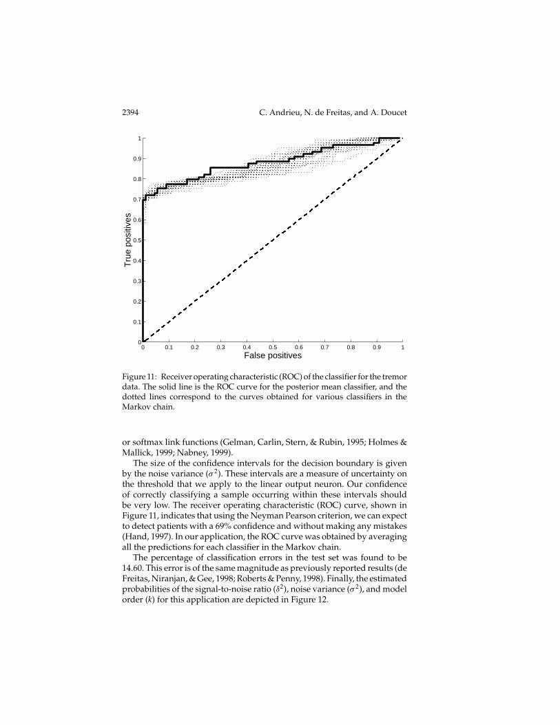
The size of the confidence intervals for the decision boundary is givenby the noise variance (σ 2). These intervals are a measure of uncertainty onthe threshold that we apply to the linear output neuron. Our confidenceof correctly classifying a sample occurring within these intervals shouldbe very low. The receiver operating characteristic (ROC) curve, shown inFigure 11, indicates that using the Neyman Pearson criterion, we can expectto detect patients with a 69% confidence and without making any mistakes(Hand, 1997). In our application, the ROC curve was obtained by averagingall the predictions for each classifier in the Markov chain.

The percentage of classification errors in the test set was found to be14.60. This error is of the same magnitude as previously reported results (deFreitas, Niranjan, & Gee, 1998; Roberts & Penny, 1998). Finally, the estimatedprobabilities of the signal-to-noise ratio (δ2), noise variance (σ 2), and modelorder (k) for this application are depicted in Figure 12.


0 100 200 300 400 500 6000

0.1

0.2

0.3

0.4δ2

0.06 0.08 0.1 0.12 0.14 0.16 0.18 0.20

0.02

0.04

0.06

σ2

0 1 2 3 4 5 6 7 8 9 100

0.2

0.4

0.6

0.8

k

Figure 12: Estimated probabilities of the signal-to-noise ratio (δ2), noise variance(σ 2), and model order (k) for the classification example.

8 Conclusions

We have proposed a robust full Bayesian model for estimating, jointly, thenoise variance, parameters, and number of parameters of an RBF model.We also considered the problem of stochastic optimization for model or-der selection and proposed a solution that makes use of a reversible-jumpsimulated annealing algorithm and classical information criteria. Moreover,we gave proofs of geometric convergence for the reversible-jump algorithmfor the full Bayesian model and convergence for the simulated annealingalgorithm.

Contrary to previously reported results, our experiments suggest thatour Bayesian model is robust with respect to the specification of the prior.In addition, we obtained more parsimonious RBF networks and slightlybetter approximation errors than the ones previously reported in the liter-ature. We also presented a comparison between Bayesian model averagingand penalized likelihood model selection with the AIC and MDL criteria.We found that the Bayesian strategy led to more accurate results. Yet the op-timization strategy using the AIC and MDL criteria and a reversible-jumpsimulated annealing algorithm was shown to converge faster for a specificcooling schedule.


There are many avenues for further research. These include estimatingthe type of basis functions required for a particular task, performing in-put variable selection, considering other noise models, adopting Bernoulliand multinomial output distributions for probabilistic classification by in-corporating ideas from the generalized linear models field, and extend-ing the framework to sequential scenarios. A solution to the first problemcan be easily formulated using the reversible-jump MCMC framework pre-sented here. Variable selection schemes can also be implemented via thereversible-jump MCMC algorithm. Finally, we are working on a sequentialversion of the algorithm that allows us to perform model selection in non-stationary environments (Andrieu, de Freitas, & Doucet, 1999a, 1999b). Wealso believe that the algorithms need to be tested on additional real-worldproblems. For this purpose, we have made the software available online athttp://www.cs.berkeley.edu/∼jfgf.

Appendix A: Notation

Ai,j: entry of the matrix A in the ith row and jth column.

A′: transpose of matrix A.

|A|: determinant of matrix A.

If z , (z1, . . . , zj−1, zj, zj+1, . . . , zk)′

then z−j , (z1, . . . , zj−1, zj+1, . . . , zk)′.

In: identity matrix of dimension n× n.

IE(z): indicator function of the set E (1 if z ∈E, 0 otherwise).

bzc: highest integer strictly less than z.

z ∼p(z): z is distributed according to p(z).

z | y ∼p(z): the conditional distribution of z given y is p(z).

Probability F fF (·)Distribution

Inverse gamma IG (α, β) βα

0(α)z−α−1 exp (−β/z) I[0,+∞) (z)

Gamma Ga (α, β) βα

0(α)zα−1 exp (−βz) I[0,+∞) (z)

Gaussian N (m, 6) |2π6|−1/2 exp(− 1

2 (z−m)′6−1 (z−m))

Poisson Pn (λ) λz

z! exp(−λ)IN (z)Uniform UA

[∫A dz

]−1 IA (z)

Appendix B: Proof of Theorem 1

The proof of theorem 1 relies on the following theorem, which is a result oftheorems 14.0.1 and 15.0.1 in Meyn and Tweedie (1993):


Theorem 3. Suppose that a Markovian transition kernel P on a space Z

1. Is a φ−irreducible (for some measure φ) aperiodic Markov transition kernelwith invariant distribution π .

2. Has geometric drift toward a small set C with drift function V: Z →[1,+∞), that is, there exists 0 < λ < 1, b > 0, k0 and an integrablemeasure ν such that:

PV(z) ≤ λV(z)+ bIC(z) (B.1)

Pk0(z, dz′) ≥ IC(z)ν(dz′). (B.2)

Then for π -almost all z0, some constants ρ < 1 and R < +∞, we have:

‖Pn(z0, ·)− π(·)‖TV ≤ RV(z0)ρn. (B.3)

That is, P is geometrically ergodic.

We need to prove five lemmas that will allow us to prove the different con-ditions required to apply theorem 2. These lemmas will enable us to proveproposition 1, which will establish the minorization condition, equation B.2,for some k0 and measure φ (to be described). The φ-irreducibility and ape-riodicity of the Markov chain are then proved in corollary 3, thereby en-suring the simple convergence of the Markov chain. To complete the proof,proposition 2 will establish the drift condition, equation B.1. To simplify thepresentation, we consider only one network output. The proof for multipleoutputs follows trivially.

Before presenting the various lemmas and their respective proofs, weneed to introduce some notation. Let K(3k1 , δ2

k1, k1, µ1:k1

; d3k2 , dδ2k2

, k2, dµ1:k2

) denote the transition kernel of the Markov chain.6 Thus, for fixed(3k1 , δ2

k1, k1, µ1:k1

) ∈ R+2 ×Ω, we have:

Pr((3k2 , δ

2k2, k2,µ1:k2

) ∈ Ak2 | (3k1 , δ2k1, k1,µ1:k1

))

=∫

Ak2

K(3k1 , δ2k1, k1,µ1:k1

; d3k2 , dδ2k2, k2, dµ1:k2

),

where Ak2 ∈ B(R+2 × k2 ×Ωk2). This transition kernel is by construction(see section 4.2) a mixture of transition kernels. Hence:

K(3k1 , δ2k1, k1,µ1:k1

; d3k2 , dδ2k2, k2, dµ1:k2

)

6 We will use the notation 3k, δ2k , when necessary, for ease of presentation. This does

not mean that these variables depend on the dimension k.


=(

bk1Kbirth(3k1 , δ2k1, k1,µ1:k1

; d3k1 , dδ2k1, k1 + 1, dµ1:k1+1)

+ dk1Kdeath(3k1 , δ2k1, k1,µ1:k1

; d3k1 , dδ2k1, k1 − 1, dµ1:k1−1)

+ sk1Ksplit(3k1 , δ2k1, k1,µ1:k1

; d3k1 , dδ2k1, k1 + 1, dµ1:k1+1)

+mk1Kmerge(3k1 , δ2k1, k1,µ1:k1

; d3k1 , dδ2k1, k1 − 1, dµ1:k1−1)

+ (1− bk1 − dk1 − sk1 −mk1)

×Kupdate(3k1 , δ2k1, k1,µ1:k1

; d3k1 , dδ2k1, k1, dµ∗1:k1

))

× p(δ2k2| δ2

k1, k2,µ1:k2

, x,y)p(3k2 | k2)d3k2 dδ2k2,

whereKbirth andKdeath correspond to the reversible jumps described in sec-tion 4.2.1,Ksplit andKmerge to the reversible jumps described in section 4.2.2,andKupdate is described in section 4.2.3. The different steps for sampling theparameters δ2

k2and 3k2 are described in section 4.1.3.

Lemma 1. We denote P∗k the matrix Pk for which δ2 → +∞. Let v ∈ RN,then v′P∗k v = 0 if and only if v belongs to the space spanned by the columns ofD(µ1:k, x

), with µ1:k ∈ Ωk.

Then, noting that y′Pky = 11+δ2 y′y + δ2

1+δ2 y′P∗k y, we obtain the followingcorollary:

Corollary 2. If the observed data y are really noisy, that is, cannot be describedas the sum of k basis functions and a linear mapping, then there exists a numberε > 0 such that for all k ≤ kmax, δ2 ∈ R+, and µ1:k ∈ Ωk, we have y′Pky ≥ε> 0.

Lemma 2. For all k ≤ kmax, δ2 ∈ R+, and µ1:k ∈ Ωk, we have y′Pky ≤ y′y.

Lemma 3. Let K1 be the transition kernel corresponding to K such that 3 andδ2 are kept fixed. Then there exists M1 > 0 such that for any M2 sufficiently large,any δ2 ∈ R+ and k1 = 1, . . . , kmax:

K1(3, δ2, k1,µ1:k1

;3, δ2, k1 − 1, dµ1:k1−1)

≥ c?I3;3<M2(3)M1M2k1

δSµ1:k1(dµ1:k1−1)

with c? > 0 as defined in equation 4.5.


Proof. According to the definition of the transition kernel, for all variables((k1,µ1:k1

), (k2,µ1:k2)) ∈ Ω2, one has the following inequality:

K1(3, δ2, k1,µ1:k1

;3, δ2, k2, dµ1:k2) ≥ min1, rdeathdk1

δSµ1:k1(dµ1:k2

)

k1,

where 1/k1 is the probability of choosing one of the basis functions for thepurpose of removing it and Sµ1:k1

, µ′ ∈ Ωk1−1/∃l ∈ 1, . . . , k1 such thatµ′ = µ−l. Then from equation 4.6 and for all k1 = 1, . . . , kmax, we have

r−1death =

(γ0 + y′1:NPk1−1y1:N

γ0 + y′1:NPk1 y1:N

)( N+υ02 ) 1

k1(1+ δ2)1/2.

As a result, we can use lemmas 1 and 2 to obtain ε and M1 such that

r−1death ≤

(γ0 + y′1:Ny1:N

ε

)( N+υ02 ) 1

k1(1+ δ2)1/2< M1 < +∞.

Thus, there exists M1 sufficiently large such that for any M2 sufficientlylarge (from equation 4.5), δ2 ∈ R+, 1 ≤ k1 ≤ kmax, and µ1:k1

∈ Ωk1

K1(3, δ2, k1,µ1:k1

;3, δ2, k1 − 1, dµ1:k1−1)

≥ I3;3<M2(3)c?

M2

1M1k1

δSµ1:k1(dµ1:k1−1). (B.4)

Lemma 4. The transition kernel K satisfies the following inequality for k = 0:

K(30, δ20, 0,µ0; d3∗0, dδ∗20 , 0, dµ0) ≥ ζϕ(δ∗20 | 0)p(30 | 0)dδ∗20 d30, (B.5)

with ζ > 0 and ϕ a probability density.

Proof. From the definition of the transition kernel K, we have:7

K(30, δ20, 0,µ0; d3∗0, dδ∗20 , 0, dµ0)

≥ u0p(δ∗20 | δ20, 0, dµ0, x,y)p(30 | 0)dδ∗20 d30

≥ (1− c?)p(δ∗20 | δ20, 0, dµ0, x,y)p(30 | 0)dδ∗20 d30

as 0 < 1− c? ≤ u0 ≤ 1, and we adopt the notation ϕ( δ∗2 | 0) , p(δ∗2 | δ2, 0,µ0, x, y).

7 When k = 0, we keep for notational convenience the same notation for the transitionkernel even if µ0 does not exist.


Lemma 5. There exists a constant ξ > 0 and a probability density ϕ such thatfor all δ2 ∈ R+, 0 ≤ k ≤ kmax, and µ1:k ∈ Ωk, one obtains:

p(δ∗2 | δ2, k,µ1:k, x,y) ≥ ξϕ(δ∗2 | k). (B.6)

Proof. From section 4.1.2, to update δ2 at each iteration, one draws fromthe distribution p(α1:m, σ

2 | δ2, k,µ1:k, x,y), that is, one draws σ 2 from

p(σ 2 | δ2, k,µ1:k, x,y)

=(γ0+y′1:NPky1:N

2

) N+υ02

0(

N+υ02

)(σ 2)

N+υ02 +1

exp( −1

2σ 2 (γ0 + y′1:NPky1:N)

);

then α1:m from

p(α1:m | δ2, k,µ1:k, σ2, x,y)

= 1|2πσ 2Mk|1/2

exp( −1

2σ 2 (α1:m − hk)′M−1

k (α1:m − hk)

);

and finally one draws δ∗2 according to

p(δ∗2 | δ2, k,θ, x,y)

=(α′1:mD′(µ1:k,x)D(µ1:k,x)α1:m

2σ 2 + βδ2

)m/2+αδ2

0(m/2+ αδ2)(δ∗2)m/2+αδ2+1

× exp(−1δ∗2

(α′1:mD′(µ1:k, x)D(µ1:k, x)α1:m

2σ 2 + βδ2

)).

Consequently:

p(δ∗2 | δ2, k,θ, x,y)p(α1:m, σ2 | δ2, k,µ1:k, x,y)

=(γ0+y′1:NPky1:N

2

) N+υ02(α′1:mD′(µ1:k,x)D(µ1:k,x)α1:m

2σ 2 + βδ2

)m/2+αδ2

0(N+υ02 )0(m/2+ αδ2)(2π)m/2(σ 2)(N+υ0+m)/2+1(δ∗2)m/2+αδ2+1|Mk|1/2

× exp( −1

2σ 2

[(α1:m − hk)

′M−1k (α1:m − hk)+ γ0 + y′1:NPky1:N

+ α′1:mD′(µ1:k, x)D(µ1:k, x)α1:m

δ∗2

]− βδ2

δ∗2

).

We can obtain the minorization condition, given by equation B.6, by inte-grating with respect to the nuisance parametersα1:m and σ 2. To accomplish


this, we need to perform some algebraic manipulations to obtain the fol-lowing relation,

(α1:m − hk)′M−1

k (α1:m − hk)+ (γ0 + y1:NPky1:N)

+ α′1:mD′(µ1:k, x)D(µ1:k, x)α1:m

δ∗2

= (α1:m − h•k)′M•−1

k (α1:m − h•k)+ γ0 + y1:NP•ky1:N,

with:

M•−1k =

(1+ 1

δ2 +1δ∗2

)D′(µ1:k, x)D(µ1:k, x)

h•k = M•kD′(µ1:k, x)y1:N

P•k = IN −D(µ1:k, x)M•kD′(µ1:k, x).

We can now integrate with respect to α1:m (gaussian distribution) and σ2

(inverse gamma distribution) to obtain the minorization condition for δ∗2:

p(δ∗2 | δ2, k,µ1:k, x,y)

≥∫Rm×R+

(γ0+y′1:NPky1:N

2

) N+υ02(βδ2)m/2+αδ2

0(N+υ02 )0(m/2+ αδ2)(2π)m/2

×(σ 2)(N+υ0+m)/2+1(δ∗2)m/2+αδ2+1|Mk|1/2

× exp( −1

2σ 2

[(α1:m − h•k)

′M•−1k (α1:m − h•k)+ γ0 + y′1:NP•ky1:N

]− βδ2

δ∗2

)dα1:mdσ 2

= |M•k |1/2

|Mk|1/2

(γ0+y′1:NPky1:N

2

) N+υ02(βδ2)m/2+αδ2

0(m/2+ αδ2)(γ0+y′1:NP•k y1:N

2

) N+υ02(δ∗2)m/2+αδ2+1

exp(−βδ2

δ∗2

)

≥(

1+ 1δ2

1+ 1δ2 + 1

δ∗2

)m/2ε

N+υ02 β

m/2+αδ2

δ2

(γ0 + y′1:Ny1:N)N+υ0

2 0(m/2+ αδ2)

1(δ∗2)m/2+αδ2+1

× exp(−βδ2

δ∗2

)

≥(

11+ δ∗2

)(kmax+d+1)/2 εN+υ0

2 mink∈0,...,kmax βm/2+α

δ2

δ2

(γ0+y′1:Ny1:N)N+υ0

2 0((kmax + d+ 1)/2+ αδ2

)


× 1

(δ∗2)kmax+d+1

2 +αδ2+1

exp(−βδ2

δ∗2

),

where we have made use of lemma 1, its corollary and lemma 2.

Proposition 1. For any M2 sufficiently large, there exists an ηM2 > 0 such thatfor all ((3k1 , δ

2k1, k1,µ1:k1

), (3k2 , δ2k2, k2,µ1:k2

)) ∈ (R+2 ×Ω)2

K(kmax)3k1 , δ21, k1,µ1:k1

; d3k2 , dδ2k2, k2, dµ1:k2

)

≥ I3k1 ;3k1<M2(3k1)ηM2φ(d3k2 , dδ2k2, k2, dµ1:k2

)

where φ(d3, dδ2, k, dµ1:k) , p(3 | k)d3ϕ(δ2 | k)dδ2I0(k)δµ0(dµ1:k).

Proof. From lemmas 3 and 5, one obtains for k1 = 1, . . . , kmax:

K(3k1 , δ2k1, k1,µ1:k1

; d3k1−1, dδ2k1−1, k1 − 1, dµk1−1)

≥ I3k1 ;3k1<M2(3k1)c?

M2

1M1k1

ξp(3k1−1 | k1 − 1)d3k1−1ϕ(δ2k1−1 | k1 − 1)

× dδ2k1−1δSµ1:k1

(dµk1−1).

Consequently for k1 = 1, . . . , kmax, when one iterates the kernel K kmaxtimes, the resulting transition kernel denoted K(kmax) satisfies:

K(kmax)(3k1 , δ2k1, k1,µ1:k1

; d3∗0, dδ∗20 , 0, dµ∗0)

=∫R+×R+×Ω

K(k1)(3k1 , δ2k1, k1,µ1:k1

; d3l, dδ2l , l, dµ1:l)K(kmax−k1)

× (3l, δ2l , l,µ1:l; d3∗0, dδ∗20 , 0, dµ∗0)

≥∫R+×R+

∫0×Ω0

K(k1)(3k1 , δ2k1, k1,µ1:k1

; d3l, dδ2l , l, dµ1:l)K(kmax−k1)

× (3l, δ2l , l,µ1:l; d3∗0, dδ∗20 , 0, dµ∗0)

= K(k1)(3k1 , δ2k1, k1,µ1:k1

; d30, dδ20, 0, dµ0)K(kmax−k1)

× (30, δ20, 0,µ0; d3∗0, dδ∗20 , 0, dµ∗0)

≥ I3k1 ;3k1<M2(3k1)Mk1−13 (

ξc?

M1M2)k1ς kmax−k1φ(d3∗0, dδ∗20 , 0, dµ∗0),

where we have used lemma 4 and M3 = mink=1,...,kmax

∫3;3<M2 p(3 | k)d3 >

0. The conclusion follows with ηM2 , minς kmax , mink∈1,...,kmaxMk−13 (

ξc?M1M2

)k

ς kmax−k > 0.


Corollary 3. The transition kernelK is φ-irreducible. In addition, we know thatp(d3, dδ2, k, dµ1:k | x,y) is an invariant distribution of K and the Markov chainis φ-irreducible; then according to Tierney (1994, theorem 1*) the Markov chainis p(d3, dδ2, k, dµ1:k | x,y)-irreducible. Aperiodicity is straightforward. Indeedthere is a nonzero probability of choosing the update move in the empty configura-tion from equation B.5 and to move anywhere in R2 × 0 × µ0. Therefore, theMarkov chain admits p(d3, dδ2, k, dµ1:k | x,y) as unique equilibrium distribution(Tierney, 1994, theorem 1*).

We will now prove the drift condition:

Proposition 2. Let V(3, δ2, k,µ1:k) , max1,3υ for υ > 0; then

lim3→+∞

KV(3, δ2, k,µ1:k)/V(3, δ2, k,µ1:k) = 0,

where by definition,

KV(3, δ2, k,µ1:k)

,∫R+×R+×Ω

K(3, δ2, k,µ1:k; d3∗, dδ∗2, k∗, dµ∗1:k)V(3∗, δ∗2, k∗,µ∗1:k)

Proof. The transition kernel of the Markov chain is of the form (we removesome arguments for convenience):

K = (bk1Kbirth + dk1Kdeath +mk1Kmerge + sk1Ksplit

+ (1− bk1 − dk1 − sk1 −mk1

)Kupdate)p(δ2

k2| δ2

k1, k2,µ1:k2

, x,y)

× p(3k2 | k2).

Now, study the following expression:

KV(3k1 , δ21, k1,µ1:k1

)

= bk1

∑k2∈k1,k1+1

∫8k2

Kbirth

∫R+

p(δ2k2| δ2

k1, k2,µ1:k2

, x,y)dδ2k2

×∫R+

p(3k2 | k2)3υk2

d3k2

+ dk1

∑k2∈k1,k1−1

∫8k2

Kdeath

∫R+

p(δ2k2| δ2

k1, k2,µ1:k2

, x,y)dδ2k2

×∫R+

p(3k2 | k2)3υk2

d3k2

+ sk1

∑k2∈k1,k1+1

∫8k2

Ksplit

∫R+

p(δ2k2| δ2

k1, k2,µ1:k2

, x,y)dδ2k2


×∫R+

p(3k2 | k2)3υk2

d3k2

+mk1

∑k2∈k1,k1−1

∫8k2

Kmerge

∫R+

p(δ2k2| δ2

k1, k2,µ1:k2

, x,y)dδ2k2

×∫R+

p(3k2 | k2)3υk2

d3k2

+ (1− bk1 − dk1 − sk1 −mk1)

∫Ωk1

Kupdate

×∫R+

p(δ∗2k1| δ2

k1, k1,µ

∗1:k1, x,y)dδ2

k1

∫R+

p(3∗k1| k1)3

∗υk1

d3∗k1

= bk1

∑k2∈k1,k1+1

∫R+

p(3k2 | k2)3υk2

d3k2

+ dk1

∑k2∈k1,k1−1

∫R+

p(3k2 | k2)3υk2

d3k2

+ sk1

∑k2∈k1,k1+1

∫R+

p(3k2 | k2)3υk2

d3k2

+mk1

∑k2∈k1,k1−1

∫R+

p(3k2 | k2)3υk2

d3k2

+ (1− bk1 − dk1 − sk1 −mk1)

∫R+

p(3∗k1| k1)3

∗υk1

d3∗k1.

As p(3 | k) is a gamma distribution, for any 0 ≤ k ≤ kmax, one obtains theinequality

∫R+ p(3 | k)3υd3 < +∞, and then the result follows immedi-

ately.

Proof of Theorem 3. By construction, the transition kernel K(3k1 , δ2k1

, k1,µ1:k1

; d3k2 , dδ2k2

, k2, dµ1:k2) admits the probability distribution p(d3, dδ2, k,

dµ1:k | x, y) as invariant distribution. Proposition 1 proved the φ-irreduc-ibility and the minorization condition with k0 = kmax, and proposition 2proved the drift condition. Thus, theorem 3 applies.

Acknowledgments

We thank Mark Coates, Bill Fitzgerald, and Jaco Vermaak (Cambridge Uni-versity), Chris Holmes (Imperial College of London), David Lowe (AstonUniversity), David Melvin (Cambridge Clinical School), Stephen Roberts,and Will Penny (University of Oxford) for very useful discussions and com-ments.


References

Akaike, H. (1974). A new look at statistical model identification. IEEE Transac-tions on Automatic Control, AC-19, 716–723.

Andrieu, C. (1998). MCMC methods for the Bayesian analysis of nonlinear paramet-ric regression models. Unpublished doctoral dissertation, University Cergy-Pontoise, Paris.

Andrieu, C., Breyer, L. A., & Doucet, A. (1999). Convergence of simulated annealingusing Foster-Lyapunov criteria (Tech. Rep. No. CUED/F-INFENG/TR 346).Cambridge: Cambridge University Engineering Department.

Andrieu, C., de Freitas, J. F. G., & Doucet, A. (1999a). Sequential Bayesian esti-mation and model selection applied to neural networks (Tech. Rep. No. CUED/F-INFENG/TR 341). Cambridge: Cambridge University Engineering Depart-ment.

Andrieu, C., de Freitas, J. F. G., & Doucet, A. (1999b). Sequential MCMC forBayesian model selection. In IEEE Higher Order Statistics Workshop (pp. 130–134), Caesarea, Israel.

Andrieu, C., Djuric, P. M., & Doucet, A. (in press). Model selection by MCMCcomputation. Signal Processing.

Bernardo, J. M., & Smith, A. F. M. (1994). Bayesian theory. New York: Wiley.Brass, A., Pendleton, B. J., Chen, Y., & Robson, B. (1993). Hybrid Monte Carlo

simulations theory and initial comparison with molecular dynamics. Biopoly-mers, 33(8), 1307–1315.

Buntine, W. L., & Weigend, A. S. (1991). Bayesian back-propagation. ComplexSystems, 5, 603–643.

Cheng, B., & Titterington, D. M. (1994). Neural networks: A review from a sta-tistical perspective. Statistical Science, 9(1), 2–54.

de Freitas, J. F. G. (1999). Bayesian methods for neural networks. Unpublished doc-toral dissertation, Cambridge University, Cambridge, UK.

de Freitas, J. F. G., Niranjan, M., & Gee, A. H. (1998). The EM algorithm andneural networks for nonlinear state space estimation (Tech. Rep. No. CUED/F-INFENG/TR 313). Cambridge: Cambridge University Engineering Depart-ment.

de Freitas, J. F. G., Niranjan, M., Gee, A. H., & Doucet, A. (2000). SequentialMonte Carlo methods to train neural network models. Neural Computation,12(4), 955–993.

Denison, D., Mallick, B. K., & Smith, A. F. M. (1998). Bayesian MARS, Statisticsand Computing, 8, 337–346.

Djuric, P. M. (1996). A model selection rule for sinusoids in white gaussian noise.IEEE Transactions on Signal Processing, 44(7), 1744–1751.

Djuric, P. M. (1998). Asymptotic MAP criteria for model selection. IEEE Trans-actions on Signal Processing, 46(10), 2726–2735.

Fahlman, S. E., & Lebiere, C. (1988). The cascade-correlation learning architec-ture. In D. S. Touretzky (Ed.), Proceedings of the Connectionist Models SummerSchool (Vol. 2, pp. 524–532) San Mateo, CA.

Frean, M. (1990). The upstart algorithm: A method for constructing and trainingfeedforward neural networks. Neural Computation, 2(2), 198–209.


Gelfand, A. E., & Dey, D. K. (1997). Bayesian model choice: Asymptotics andexact calculations. Journal of the Royal Statistical Society B, 56(3), 501–514.

Gelman, A., Carlin, J. B., Stern, H. S., & Rubin, D. B. (1995). Bayesian data analysis.London: Chapman and Hall.

Geman, S., & Geman, D. (1984). Stochastic relaxation, Gibbs distributions andthe Bayesian restoration of images. IEEE Transactions on Pattern Analysis andMachine Intelligence, 6(6), 721–741.

George, E. I., & Foster, D. P. (1997). Calibration and empirical Bayes variable se-lection. Unpublished manuscript, Department of Management Science andInformation Systems, University of Texas.

Gilks, W. R., Richardson, S., & Spiegelhalter, D. J. (Eds.). (1996). Markov chainMonte Carlo in practice. London: Chapman and Hall.

Girosi, F., Jones, M., & Poggio, T. (1995). Regularization theory and neural net-works architectures. Neural Computation, 7(2), 219–269.

Green, P. J. (1995). Reversible jump Markov chain Monte Carlo computation andBayesian model determination. Biometrika, 82, 711–732.

Hand, D. J. (1997). Construction and assessment of classification rules. New York:Wiley.

Hinton, G. (1987). Learning translation invariant recognition in massively par-allel networks. In J. W. de Bakker, A. J. Nijman, & P. C. Treleaven (Eds.),Proceedings of the Conference on Parallel Architectures and Languages (pp. 1–13)Berlin.

Holmes, C. C., & Mallick, B. K. (1998). Bayesian radial basis functions of variabledimension. Neural Computation, 10(5), 1217–1233.

Holmes, C. C., & Mallick, B. K. (1999). Generalised nonlinear modelling with multi-variate smoothing splines. Unpublished manuscript, Statistics Section, Depart-ment of Mathematics, Imperial College of London.

Holmes, C. C., & Mallick, B. K. (2000). Bayesian wavelet networks for nonpara-metric regression. IEEE Transactions on Neural Networks, 11(1), 27–35.

Kadirkamanathan, V., & Niranjan, M. (1993). A function estimation approach tosequential learning with neural networks. Neural Computation, 5(6), 954–975.

Le Cun, Y., Denker, J. S., & Solla, S. A. (1990). Optimal brain damage. In D. S.Touretzky (Ed.), Advances in neural information processing systems, 2 (pp. 598–605). San Mateo, CA: Morgan Kaufmann.

Mackay, D. J. C. (1992). A practical Bayesian framework for backpropagationnetworks. Neural Computation, 4(3), 448–472.

Marrs, A. D. (1998). An application of reversible-jump MCMC to multivariatespherical Gaussian mixtures. In M. I. Jordan, M. J. Kearns, & S. A. Solla (Eds.),Advances in neural information processing systems, 10 (pp. 577–583). Cambridge,MA: MIT Press.

Meyn, S. P., & Tweedie, R. L. (1993). Markov chains and stochastic stability. NewYork: Springer-Verlag.

Moody, J., & Darken, C. (1988). Learning with localized receptive fields. InG. Hinton, T. Sejnowski, & D. Touretzsky (Eds.), Proceedings of the 1988 Con-nectionist Models Summer School (pp. 133–143). Palo Alto, CA.

Muller, P., & Rios Insua, D. (1998). Issues in Bayesian analysis of neural networkmodels. Neural Computation, 10, 571–592.


Nabney, I. T. (1999). Efficient training of RBF networks for classification (Tech. Rep.No. NCRG/99/002). Birmingham, UK: Neural Computing Research Group,Aston University.

Neal, R. M. (1996). Bayesian learning for neural networks. New York: Springer-Verlag.

Platt, J. (1991). A resource allocating network for function interpolation. NeuralComputation, 3, 213–225.

Richardson, S., & Green, P. J. (1997). On Bayesian analysis of mixtures with anunknown number of components. Journal of the Royal Statistical Society B,59(4), 731–792.

Rios Insua, D., & Muller, P. (1998). Feedforward neural networks for nonpara-metric regression. In D. K. Dey, P. Muller, & D. Sinha (Eds.), Practical nonpara-metric and semiparametric Bayesian statistics (pp. 181–191). New York: SpringerVerlag.

Rissanen, J. (1987). Stochastic complexity. Journal of the Royal Statistical Society,49, 223–239.

Robert, C. P., & Casella, G. (1999). Monte Carlo statistical methods. New York:Springer-Verlag.

Roberts, S. J., & Penny, W. D. (1998). Bayesian neural networks for classification:How useful is the evidence framework? Neural Networks, 12, 877–892.

Roberts, S. J., Penny, W. D., & Pillot, D. (1996). Novelty, confidence and errorsin connectionist systems. IEE Colloquium on Intelligent Sensors and Fault De-tection, no. 261, 10/1–10/6.

Schwarz, G. (1985). Estimating the dimension of a model. Annals of Statistics,6(2), 461–464.

Smith, M., & Kohn, R. (1996). Nonparametric regression using Bayesian variableselection. Journal of Econometrics, 75(2), 317–343.

Spyers-Ashby, J. M., Bain, P., & Roberts, S. J. (1998). A comparison of fast Fouriertransform (FFT) and autoregressive (AR) spectral estimation techniques forthe analysis of tremor data. Journal of Neuroscience Methods, 83(1), 35–43.

Tierney, L. (1994). Markov chains for exploring posterior distributions. The An-nals of Statistics, 22(4), 1701–1762.

Van Laarhoven, P. J., & Arts, E. H. L. (1987). Simulated annealing: Theory andapplications, Amsterdam: Reidel P.

Vapnik, V. (1995). The Nature of statistical learning theory. New York: Springer-Verlag.

Yingwei, L., Sundararajan, N., & Saratchandran, P. (1997). A sequential learn-ing scheme for function approximation using minimal radial basis functionneural networks. Neural Computation, 9, 461–478.

Zellner, A. (1986). On assessing prior distributions and Bayesian regression anal-ysis with g-prior distributions. In P. Goel & A. Zellner (Eds.), Bayesian inferenceand decision techniques (pp. 233–243) Amsterdam: Elsevier.

Received August 25, 1999; accepted November 17, 2000.

Robust Full Bayesian Learning for Radial Basis Networksnando/papers/neuralNetMCMC.pdf · Robust Full Bayesian Learning for Radial Basis Networks ... optimize neural networks. This

Documents