Robust estimation of error scale in nonparametric regression models

Robust Estimation of Error Scale in

Nonparametric Regression Models

Isabella Rodica GhementUniversity of British Columbia

[email protected]

Marcelo RuizUniversidad Nacional de Rıo Cuarto

[email protected]

Ruben ZamarUniversity of British Columbia

[email protected]

December 22, 2007

Abstract

When the data used to fit a nonparametric regression model are contaminated with outliers, we need to use a

robust estimator of scale in order to make robust estimation of the regression function possible. We develop a

family of M-estimators of scale constructed from consecutive differences of regression responses. Estimators

in our family robustify the estimator proposed by Rice (1984). Under appropriate conditions, we establish the

weak consistency and asymptotic normality of all estimators in our family. Estimators in our family vary in

terms of their robustness properties. We quantify the robustness of each estimator via the maxbias. We use

this measure as a basis for deriving the asymptotic breakdown point of the estimator. Our theoretical results

allow us to specify conditions for estimators in our family to achieve a maximum asymptotic breakdown

point of 1/2. We conduct a simulation study to compare the finite sample performance of our preferred

M-estimator with that of three other estimators.

Keywords and Phrases: Asymptotic breakdown point, consecutive differences, error scale, fixed design,

maxbias, M-scale estimator, M-scale functional, nonparametric regression, outliers, robust.

1

1. Introduction

Robust estimators of error scale are widely used in nonparametric regression with outliers. In partic-

ular, such estimators are needed to compute robust M-estimators of the regression curve (see Hardle

and Gasser, 1984, Hardle and Tsybakov, 1988, Boente and Fraiman, 1989, and references therein).

Other applications include outliers detection (see Hannig and Lee, 2006), robust bandwidth selection

for accurate estimation of the regression curve (see, for example, Boente, Fraiman and Meloche, 1997;

Leung, Marriott and Wu, 1993; Cantoni and Ronchetti, 2001 and Leung, 2005) and robust inference

about the regression curve.

Several authors considered the problem of error scale estimation in the context of outlier-free

nonparametric regression. Dette, Munk and Wagner (1998) give an exhaustive discussion of the

various estimators of error scale available in the literature and note that the most popular estimators

are based on differences of regression responses. Since they do not rely on preliminary estimation of

the regression curve itself, these difference-based estimators have fast√n-convergence rate and are

computationally convenient. However, such estimators do not perform well in the presence of outliers.

In this paper, we introduce a family of robust M-estimators of error scale constructed from consec-

utive differences of regression responses. Our family includes the estimator proposed by Rice (1984)

and its robustified version proposed by Boente, Fraiman and Meloche (1997) as particular cases. Un-

der appropriate regularity conditions, we establish the weak consistency and asymptotic normality

of all estimators in our family. These estimators differ in terms of their robustness properties. We

quantify the robustness of each estimator via its so-called maxbias. We rely on maxbias to derive the

asymptotic breakdown point of each estimator. As far as we are aware, all the proposed estimators of

error scale based on differences fail to achieve maximum asymptotic breakdown point of 1/2. Using

our theoretical results we are able to specify conditions for estimators in our family to achieve an

asymptotic breakdown point of 1/2.

The rest of the paper is organized as follows. In Section 2, we introduce the nonparametric

regression model of interest in this paper and identify the relevant scale parameter for this model.

In Section 3, we define a family of M-estimators for this scale parameter and we we introduce the

family of M-scale functionals associated with the family of M-estimators. In Section 4, we show

that each M-estimator in our family is weakly consistent to its corresponding M-functional and has

an asymptotically normal distribution. In Section 5, we investigate the robustness properties of the

estimators in our family. In Section 6, we conduct a simulation study to compare the finite sample

2

performance of our preferred estimator against three competing estimators, including the estimators

of Rice (1984) and Boente, Fraiman and Meloche (1997). Section 7 provides some concluding remarks.

All the proofs, figures and tables are collected in the Appendix.

2. Nonparametric Regression Model

The nonparametric regression model of interest in this paper can be expressed as

Yi = g(xi) + Ui, i = 1, . . . , n, (1)

where the Yi’s are observed responses, the xi’s are fixed design points, g(·) is an unknown, smooth

regression function and the Ui’s are independent, identically distributed unobservable random errors.

We assume that the majority of the observations Yi in model (1) is of good quality and has constant

variability about the regression function g(·), but a fraction ε is possibly of bad quality. We formalize

this assumption below.

Let G denote the distribution function of the Ui’s. Then G belongs to the ε-contaminated neigh-

bourghood:

Fε = {G ∈ D : G(y) = (1− ε)F (y) + εH(y)}. (2)

Here, D denotes the set of all distribution functions, F belongs to the scale family associated with

some fixed distribution function F0, that is, F (y) = F0(y/σ) for an unspecified scale parameter σ > 0,

H is an arbitrary contaminating distribution function in D and ε ∈ [0, 1/2] denotes the amount of

contamination. Throughout, we assume that F0 admits a symmetric, strictly positive and unimodal

density f0 and H is absolutely continuous.

Remark 1. The restriction to absolutely continuous contaminating distributions simplifies the proofs

of the robustness properties of the M estimators of σ introduced in Section 3; these proofs can be

found in the Appendix. Since many distributions, including point masses, can be arbitrarily well

approximated by absolutely continuous distributions, the considered family seems broad enough for

practical purposes.

Our interest is in robustly estimating the scale parameter σ from the sequence of consecutive

3

differences Yi+1 − Yi, i = 1, . . . , n− 1. Note that σ is not only unambiguously defined, but also fixed

across the neighbourhood Fε.

3. M-Estimator of Error Scale

To estimate the scale parameter σ of the central distribution F in (2), we propose using a regression-

free estimator, constructed from the sequence of consecutive differences Yi+1 − Yi, i = 1, . . . , n − 1.

This estimator, referred to as an M-scale estimator, is defined as

σn = inf

{s > 0 :

1

n− 1

n−1∑

i=1

χ

(Yi+1 − Yi

as

)≤ b

}. (3)

The score function χ : R → [0,∞) must be chosen by the user and the constants b ∈ (0, 1) and

a ∈ (0,∞) are tuning constants that satisfy

E[χ(Z1)] = b (4)

and

E

[χ

(Z2 − Z1

a

)]= b, (5)

where Z1, Z2 are independent random variables with common distribution F0.

The infimum in (3) is needed to handle situations where the score function χ is discontinuous. If

χ is continuous, then σn satisfies:

1

n− 1

n−1∑

i=1

χ

(Yi+1 − Yiaσn

)= b. (6)

If, in addition, χ is strictly increasing on {x : χ(x) < supx

χ(x)}, then σn is uniquely defined by (6).

Also, the M-estimator σn = σn(Y1, . . . , Yn) is scale equivariant, in the sense that, for any c ∈ R, it

satisfies σn(cY1, . . . , cYn) = |c| σn(Y1, . . . , Yn).

Note that σn is a generic member of a family of M -estimators, whose particular members corre-

spond to different choices of the score function χ and the tuning constants a and b. In this paper,

we show that the choice of χ is not very crucial to ensuring that σn achieves the desired robustness

4

properties (as long as χ is smooth and bounded), but the choice of b is (see Section 5). Given b, a is

chosen so that σn is Fisher-consistent when there is no contamination in the data (see Section 4).

The examples below illustrate various choices of χ, b and a for the case when F0 = Φ, where Φ is

the standard normal distribution function.

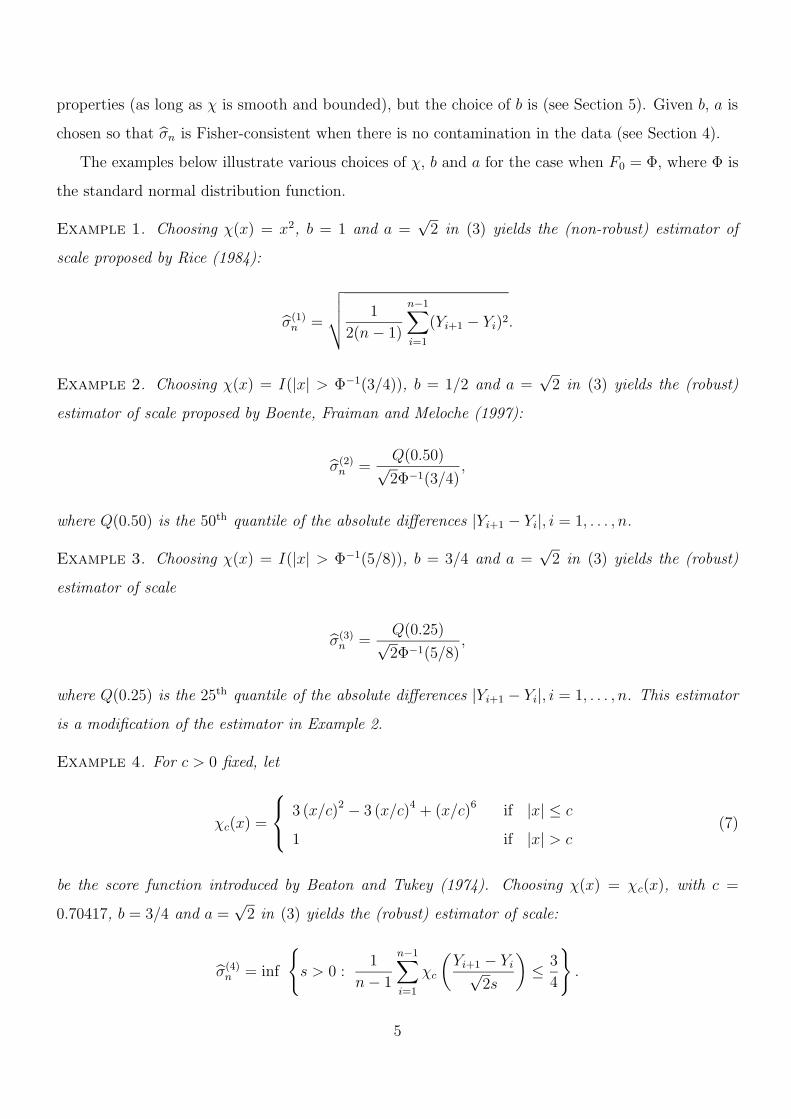
Example 1. Choosing χ(x) = x2, b = 1 and a =√2 in (3) yields the (non-robust) estimator of

scale proposed by Rice (1984):

σ(1)n =

√√√√ 1

2(n− 1)

n−1∑

i=1

(Yi+1 − Yi)2.

Example 2. Choosing χ(x) = I(|x| > Φ−1(3/4)), b = 1/2 and a =√2 in (3) yields the (robust)

estimator of scale proposed by Boente, Fraiman and Meloche (1997):

σ(2)n =

Q(0.50)√2Φ−1(3/4)

,

where Q(0.50) is the 50th quantile of the absolute differences |Yi+1 − Yi|, i = 1, . . . , n.

Example 3. Choosing χ(x) = I(|x| > Φ−1(5/8)), b = 3/4 and a =√2 in (3) yields the (robust)

estimator of scale

σ(3)n =

Q(0.25)√2Φ−1(5/8)

,

where Q(0.25) is the 25th quantile of the absolute differences |Yi+1 − Yi|, i = 1, . . . , n. This estimator

is a modification of the estimator in Example 2.

Example 4. For c > 0 fixed, let

χc(x) =

3 (x/c)2 − 3 (x/c)4 + (x/c)6 if |x| ≤ c

1 if |x| > c(7)

be the score function introduced by Beaton and Tukey (1974). Choosing χ(x) = χc(x), with c =

0.70417, b = 3/4 and a =√2 in (3) yields the (robust) estimator of scale:

σ(4)n = inf

{s > 0 :

1

n− 1

n−1∑

i=1

χc

(Yi+1 − Yi√

2s

)≤ 3

4

}.

5

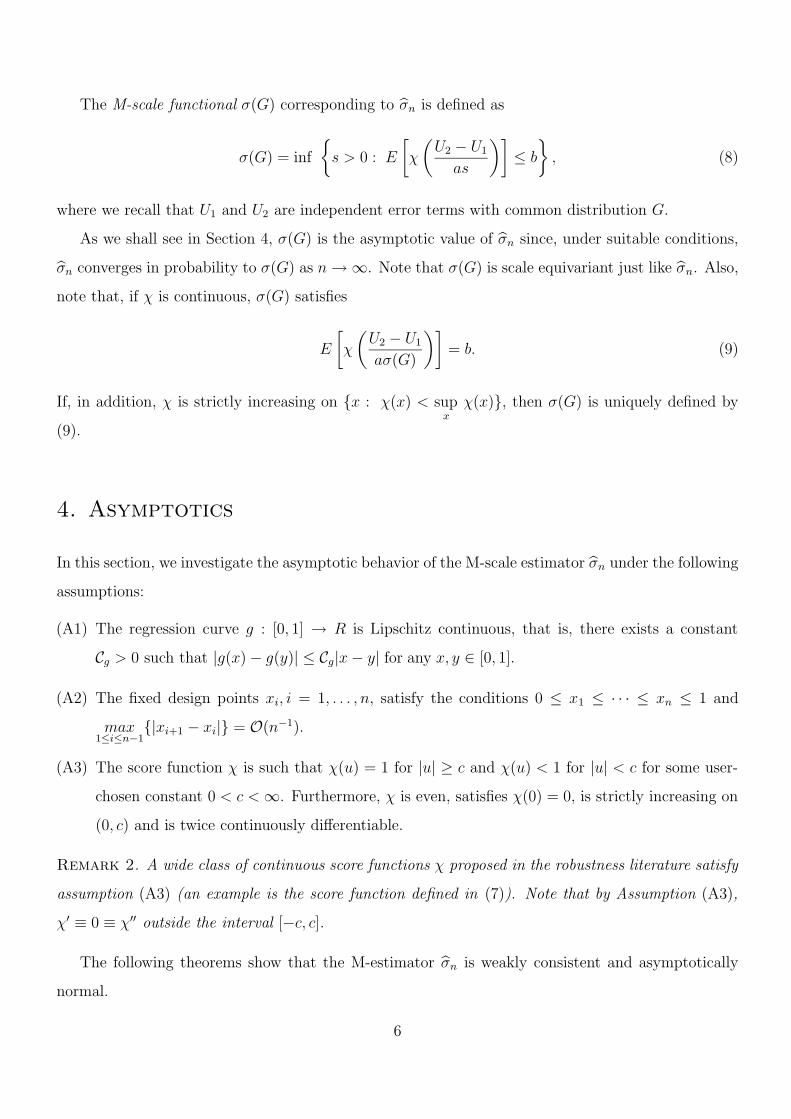
The M-scale functional σ(G) corresponding to σn is defined as

σ(G) = inf

{s > 0 : E

[χ

(U2 − U1

as

)]≤ b

}, (8)

where we recall that U1 and U2 are independent error terms with common distribution G.

As we shall see in Section 4, σ(G) is the asymptotic value of σn since, under suitable conditions,

σn converges in probability to σ(G) as n→∞. Note that σ(G) is scale equivariant just like σn. Also,

note that, if χ is continuous, σ(G) satisfies

E

[χ

(U2 − U1

aσ(G)

)]= b. (9)

If, in addition, χ is strictly increasing on {x : χ(x) < supx

χ(x)}, then σ(G) is uniquely defined by

(9).

4. Asymptotics

In this section, we investigate the asymptotic behavior of the M-scale estimator σn under the following

assumptions:

(A1) The regression curve g : [0, 1] → R is Lipschitz continuous, that is, there exists a constant

Cg > 0 such that |g(x)− g(y)| ≤ Cg|x− y| for any x, y ∈ [0, 1].

(A2) The fixed design points xi, i = 1, . . . , n, satisfy the conditions 0 ≤ x1 ≤ · · · ≤ xn ≤ 1 and

max1≤i≤n−1

{|xi+1 − xi|} = O(n−1).

(A3) The score function χ is such that χ(u) = 1 for |u| ≥ c and χ(u) < 1 for |u| < c for some user-

chosen constant 0 < c <∞. Furthermore, χ is even, satisfies χ(0) = 0, is strictly increasing on

(0, c) and is twice continuously differentiable.

Remark 2. A wide class of continuous score functions χ proposed in the robustness literature satisfy

assumption (A3) (an example is the score function defined in (7)). Note that by Assumption (A3),

χ′ ≡ 0 ≡ χ′′ outside the interval [−c, c].

The following theorems show that the M-estimator σn is weakly consistent and asymptotically

normal.

6

Theorem 1. Let {Yi}ni=1 be independent random variables satisfying (1). Then, under the Assump-

tions (A1) - (A3), σnP−→ σ(G), as n→∞ (where

P−→ denotes convergence in probability).

Theorem 2. Let {Yi}ni=1 be independent random variables satisfying (1). Set

V1(G) = V ar

[χ

(U2 − U1

aσ(G)

)], V2(G) = 2Cov

[χ

(U2 − U1

aσ(G)

), χ

(U3 − U2

aσ(G)

)]

V3(G) = E

[χ ′(U2 − U1

aσ(G)

)(U2 − U1

aσ(G)2

)]

where Ui, i = 1, 2, 3 are independent error terms with common distribution G. Then, under the As-

sumptions (A1) - (A3), we have√n (σn − σ(G))

d−→ N(0, V (G)), as n→∞, where the Asymptotic

Variance is given by V (G) = (V1(G) + V2(G))/V 23 (G) (

d−→ denotes convergence in distribution).

5. Robustness Properties

In this section, we consider the maximum generalized asymptotic bias (or maxbias) of σn as the most

complete and accurate measure for assessing the robustness of σn. We then use this measure as a

basis for our asymptotic breakdown point considerations regarding σn.

5.1. Generalized Asymptotic Bias

When there is no contamination in the data, that is, when ε = 0, the distribution function of the

errors in model (1) is F . In this case, we would like to be able to estimate σ, the scale parameter of

F , without bias. This leads to the notion of Fisher-consistency: we say that σ(G) is Fisher-consistent

for G = F if σ(F ) = σ. It is easy to see that the choices of b and a given in (4) and (5), respectively,

ensure the Fisher-consistency of σ(G) for G = F .

However, Theorem 1 suggests that σn is asymptotically biased when the data are contaminated,

as it converges in probability to σ(G) instead of σ as n → ∞. That is, in general, if G 6= F , then

σ(G) 6= σ.

The raw asymptotic bias of σn quantifies the distance between σ(G), the asymptotic value of σn,

and σ, the scale parameter of interest, and is defined as Br(σ(G)) = σ(G)σ− 1. If G is an outliers

7

generating distribution, the raw asymptotic bias is likely positive. If G is an inliers generating

distribution, the raw asymptotic bias is likely negative.

A more useful measure for assessing the asymptotic bias of σn is the generalized asymptotic bias

of this estimator, defined as

Bg(σ(G)) =

L1

(σ(G)σ

), if 0 < σ(G) ≤ σ,

L2

(σ(G)σ

), if σ < σ(G) <∞.

The functions L1 and L2 allow the user to penalize under-estimation and over-estimation of σ in

different ways. Both functions are assumed to be non-negative, continuous, monotone and to satisfy

the conditions L1(1) = L2(1) = 0 and lims↘0

L1(s) = lims→∞

L2(s) =∞.

A robust estimator σn can be expected to have a relatively small and stable generalized asymptotic

bias Bg(σ(G)) as G ranges over Fε. The overall bias performance of σn on the neighbourhood Fε can

thus be measured by the maximum generalized asymptotic bias (maxbias):

Bg(ε) = supG∈Fε

Bg(σ(G)). (10)

Note that Bg(ε) is scale invariant since the M-scale functional σ(G) is scale equivariant. Also, note

that the maxbias is a function that depends on ε, the fraction of contamination in the data. The

maxbias curve, obtained by plotting Bg(ε) versus ε, can be used to visually assess the robustness

properties of σn. We consider σn to be robust if Bg(ε) <∞ for some ε ∈ (0, 1/2].

To derive an explicit expression for Bg(ε), let

S+(ε) = supG∈Fε

σ(G) and S−(ε) = infG∈Fε

σ(G) (11)

be the maximum and minimum values of the M-scale functional σ(G) over Fε, respectively. Then,

using the monotonicity of L1 and L2, Bg(ε) can be expressed as:

Bg(ε) = max

{L1

(S−(ε)

σ

), L2

(S+(ε)

σ

)}. (12)

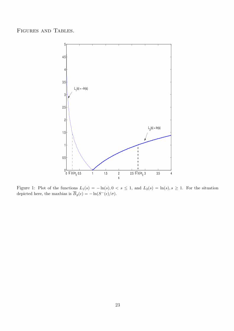
To visually illustrate the concept of maxbias, we refer to Figure 1 in the Appendix, which displays

a plot of the functions L1(s) = − ln(s), s ∈ (0, 1] and L2(s) = ln(s), s ∈ [1,∞). For the situation

depicted in this figure, Bg(ε) = − ln(S−(ε)/σ).

8

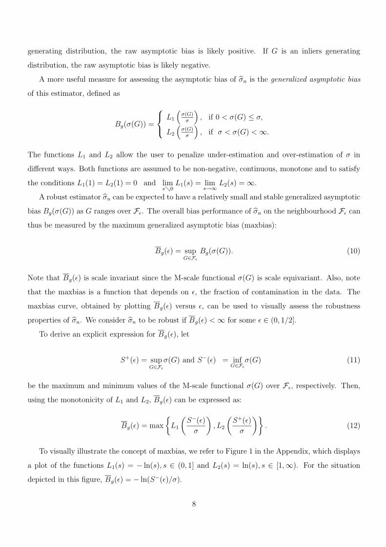
5.2. Asymptotic Breakdown Point Considerations

If the amount of contamination in the data is too large, σn can suffer two types of breakdown: it can

either explode, in the sense of taking on arbitrarily large aberrant values, or implode, in the sense of

taking on arbitrarily small aberrant values.

The asymptotic explosion breakdown point of σn is defined as ε∞ = inf{ε ∈ (0, 1/2] : S+(ε) =∞}whereas its asymptotic implosion breakdown point is defined as ε0 = inf{ε ∈ (0, 1/2] : S−(ε) = 0}.

The overall asymptotic breakdown point of σn is defined as the minimum of the asymptotic implo-

sion and explosion breakdown points ε∗ = min{ε0, ε∞}.Clearly, if the amount of contamination in the data exceeds the overall asymptotic breakdown

point of σn, then σn ceases to provide a useful summary for the scale of the uncontaminated errors.

Note that

ε∗ = inf{ε ∈ (0, 1/2] : Bg(ε) =∞

}(13)

since Bg(ε) =∞ if and only if S−(ε) = 0 or S+(ε) =∞.

The overall asymptotic breakdown point of σn depends on the value of the tuning constant b in

(3). What is the maximum overall asymptotic breakdown point that can be achieved by σn as the

value of b varies? Based on (13), to answer this question we must first derive an explicit expression

for Bg(ε).

In view of (12), to obtain an explicit expression for Bg(ε) it suffices to obtain explicit expressions

for S+(ε) and S−(ε). Such expressions are provided in Propositions 1 and 2 below, whose proofs can

be found in the Appendix. For Propositions 1 and 2 and the subsequent results in this section, we

assume without loss of generality that σ = 1.

Proposition 1. Let S+(ε) be as in (11), with ε ∈ (0, 1/2] fixed. Then, provided assumption (A3)

holds, we have:

S+(ε) =

s+(ε) if ε(2− ε) < b

∞ if ε(2− ε) ≥ b

where s+(ε) is implicitly defined by

λ+(s+(ε)) = 0. (14)

9

Here,

λ+(s) = (1− ε)2E

[χ

(Z2 − Z1

as

)]+ ε(2− ε)− b, (15)

and Z1, Z2 are independent random variables with common distribution F0.

Remark 3. By (iii) of Lemma 5 in the Appendix, the equation λ+(s) = 0 admits a unique, strictly

positive solution for those ε ∈ (0, 1/2] with ε(2− ε) < b. Therefore, the quantity s+(ε) satisfying (14)

exists and is uniquely defined.

Proposition 2. Let S−(ε) be as in (11), with ε ∈ (0, 1/2] fixed. If assumption (A3) holds, then

S−(ε) =

s−(ε) if 1− ε2 > b

0 if 1− ε2 ≤ b

where s−(ε) is implicitly defined by

λ−(s−(ε)) = 0. (16)

Here,

λ−(s) = (1− ε)2E

[χ

(Z2 − Z1

as

)]+ 2ε(1− ε)E

[χ

(Z1

as

)]− b, (17)

and Z1, Z2 are as in Proposition 1.

Remark 4. By (iii) of Lemma 6 in the Appendix, the equation λ−(s) = 0 admits a unique, strictly

positive solution for those ε ∈ (0, 1/2] for which 1− ε2 > b, so the quantity s−(ε) satisfying (16) exists

and is uniquely defined.

The next theorem provides an explicit expression for Bg(ε), the maxbias of σn over Fε. This

theorem is proven in the Appendix.

Theorem 3. Assume that the notation and assumptions in Propositions 1 and 2 hold. For ε ∈(0, 1/2], let Bg(ε) be as in (10). Also, let b ∈ (0, 1) be a tuning constant satisfying (3). The following

facts hold.

10

(i) If b = 3/4, then

Bg(ε) =

max{L2(s+(ε)), L1(s

−(ε))} if ε < 1/2,

∞ if ε = 1/2.

(ii) If b ∈ (0, 3/4), then

Bg(ε) =

max{L2(s+(ε)), L1(s

−(ε))} if ε < 1−√1− b,

∞ if 1−√1− b ≤ ε.

(iii) If b ∈ (3/4, 1), then

Bg(ε) =

max{L2(s+(ε)), L1(s

−(ε))} if ε <√1− b,

∞ if√1− b ≤ ε.

As an immediate consequence of the above theorem, we derive an explicit expression for the overall

asymptotic breakdown point of σn as a function of b:

Theorem 4. Let ε∗ be the overall asymptotic breakdown point of σn defined by (13). Also, let

b ∈ (0, 1) be the tuning constant in (3).

(i) If b = 3/4, then ε∗ = 1/2.

(ii) If b ∈ (0, 3/4), then ε∗ = 1−√1− b.

(iii) If b ∈ (3/4, 1), then ε∗ =√1− b.

Corollary 1. The maximum overall asymptotic breakdown point that can be achieved by σn as the

value of the tuning constant b in (3) varies in the interval (0, 1) is ε∗opt = 1/2; this optimal asymptotic

breakdown point is attained for b = 3/4.

So far, we have investigated the robustness properties of the M-estimator σn for a general score

function χ satisfying assumption (A3). In practice, χ must be specified by the user. One particular

choice of χ that we recommend and that satisfies assumption (A3) is the score function χc in (7). The

tuning constant c > 0 should be chosen to ensure that: (i) σn achieves the optimal overall asymptotic

breakdown point and (ii) σn’s limiting value, σ(G), is Fisher-consistent when G = F , that is, when

11

there is no contamination in the data. In what follows, we explain how to choose c for the case when

F0 is the standard normal distribution function Φ.

Recall from Corollary 1 that we should choose b = 3/4 to ensure that σn achieves the optimal

asymptotic breakdown point of 1/2. According to the Fisher-consistency considerations in Section 3,

to ensure that σ(G) is Fisher-consistent when G = F , we must choose c so that

E [χc(Z1)] = b,

where Z1 ∼ N(0, 1). One can easily see that c = 0.70417 satisfies the above equality.

Remark 5 We emphasize that we only consider the asymptotic breakdown point under the model

of independent contamination. In this setup our estimators can attain the maximal breakdown point

0.5. This is no longer the case when we consider the finite sample setup where one can construct

particularly damaging outlier configurations (e.g. ε · 100% intercalated outliers would spoil 2ε · 100%of the differences). However, these outlier configurations have zero limiting probability under the

independent contamination model.

6. Simulations

In this section, we report the results of a Monte Carlo simulation study on the finite sample properties

of the estimators σ(1)n , σ

(2)n , σ

(3)n and σ

(4)n introduced in Examples 1 to 4.

The main goals of the study are to: (i) investigate the efficiency properties of σ(2)n , σ

(3)n and σ

(4)n

relative to σ(1)n in the absence of outlier contamination and (ii) compare the mean squared error

performance of the four estimators in the presence of outlier contamination.

First we consider the model of independent contaminations and, in a second stage, we study a

model of intercalated contaminated responses using point mass contaminations as outliers. Figures

and tables are in the Appendix.

For our simulation study we generate data from model (1) as follows. We take n = 20, 50 and

100. We consider g(x) = sin(4πx). We take xi = (i − 1)/(n − 1), i = 1, . . . , n. We consider the

error terms Ui’s to arise from two contamination scenarios: (I) the independent contamination model

described in Section 2, and (II) an intercalated contamination model. For (I) the Ui’s have common

12

distribution G = (1 − ε)F + εH, where F (·) = Φ(·/σ) and σ = 1. Further, we use H(y) = Φ(y/10)

to model symmetric outliers and H(y) = Φ(y− 10) to model asymmetric outlier. For (II) we assume

that the Ui’s are as follows: U2i−1 ∼ ∆10(y) for i ∈ C = Cn,ε = {1, 2, . . . , [n · ε]} and Ui ∼ Φ otherwise

(∆10 is the point mass distribution at 10 and [a] denotes the integer part of a). For each model

configuration, we generate 10, 000 data sets.

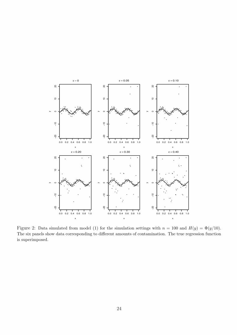
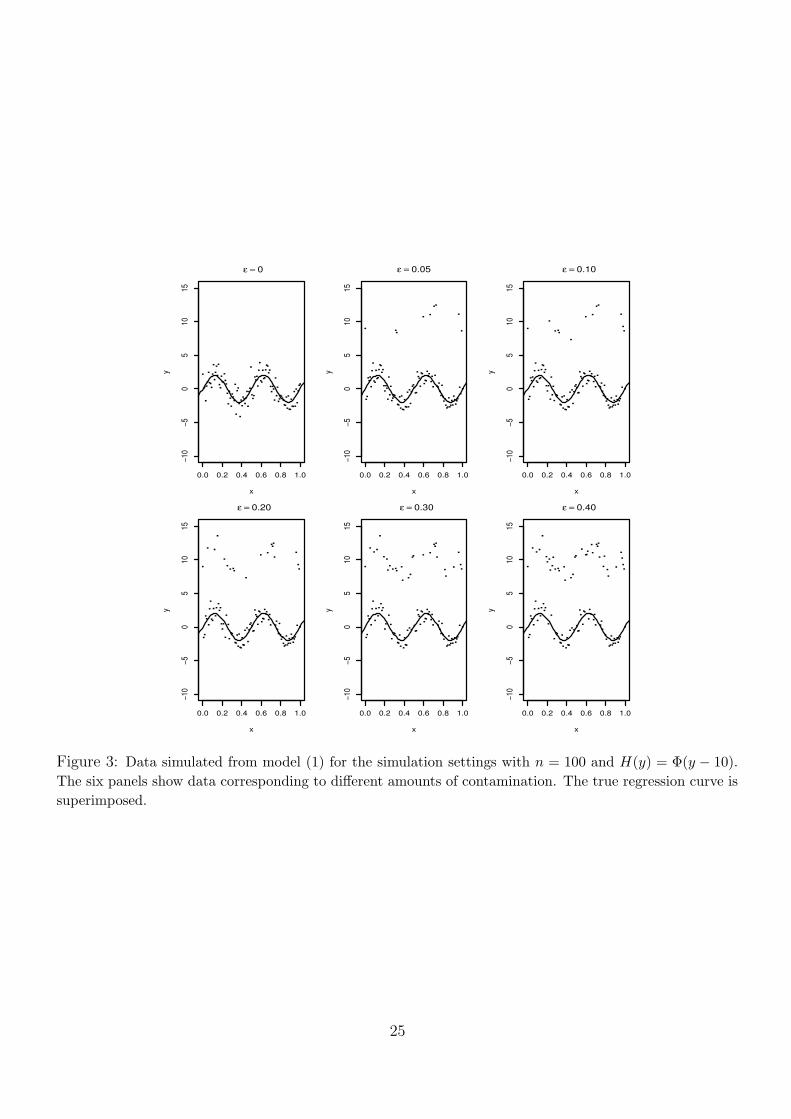
Figure 2 displays data generated for simulation settings with n = 100 andH(y) = Φ(y/10). Figure

3 provides the same display for simulation settings with n = 100 and H(y) = Φ(y−10). As expected,

the two figures reveal that the larger the amount of contamination ε, the more outliers are present

in the data. When the contamination is symmetric, the outliers tend to be located both below and

above the true regression curve. However, when the contamination is asymmetric, the outliers are

concentrated exclusively above the regression curve.

Before studying the finite sample properties of the estimators σ(1)n , σ

(2)n , σ

(3)n and σ

(4)n , we make

some considerations regarding their overall asymptotic breakdown points. The overall asymptotic

breakdown point of σ(1)n is 0, as this estimator uses an unbounded score function. The overall asymp-

totic breakdown point of σ(4)n was determined in Section 5 to be 1/2. We do not have theoretical

results concerning the exact value of the overall asymptotic breakdown point for σ(2)n and σ

(3)n . The

reason for this is that, unlike σ(4)n , both of these estimators are computed with discontinuous score

functions. Nevertheless, given that these score functions can be easily adjusted to become twice

continuously differentiable, we expect the asymptotic breakdown point considerations in Section 5 to

hold, at least approximately, for σ(2)n and σ

(3)n . Therefore, we conjecture that σ

(2)n ’s overall asymptotic

breakdown point is roughly 0.29 (use Theorem 4 with b = 1/2), while σ(3)n ’s is roughly 1/2 (use

Theorem 4 with b = 3/4). Our conjecture is supported by the simulation results reported in this

section.

We now assess the efficiency of the robust estimators σ(2)n , σ

(3)n and σ

(4)n relative to the non-robust

estimator σ(1)n for those simulation settings with ε = 0. For j = 2, 3, 4 fixed, we evaluate the efficiency

of σ(j)n relative to σ

(1)n by computing the ratio RE(σ

(j)n , σ

(1)n ) = V ar(σ

(j)n )/V ar(σ

(1)n ), where

V ar(σ(j)n ) =

1

10, 000

10,000∑

i=1

(σ

(j)n,i − σn

(j))2

.

Here, σ(j)n,i is the value of σ

(j)n corresponding to the ith sample generated from the model configuration

of interest and σn(j)

=∑10,000

i=1 σ(j)n,i/10, 000 . Notice that both σ

(3)n and σ

(4)n have roughly the same

13

overall asymptotic breakdown point, so comparing their relative efficiencies is appropriate. Comparing

the relative efficiency of σ(2)n against that of σ

(3)n and σ

(4)n may however not be appropriate as σ

(2)n has

a much smaller overall asymptotic breakdown point than both σ(3)n and σ

(4)n .

Table 1 displays the values of RE(σ(j)n , σ

(1)n ), j = 2, 3, 4, for the simulation settings with ε = 0.

From this table, we see that σ(2)n attains slightly better relative efficiency than σ

(3)n and σ

(4)n at

the expense of robustness by achieving only 29% overall asymptotic breakdown point instead of 50%.

However, σ(3)n and σ

(4)n have much better robustness properties and not much worse relative efficiencies

than σ(2)n , so we prefer them to σ

(2)n .

Next, we compare the mean squared error performance of the estimators σ(1)n ,σ

(2)n , σ

(3)n and σ

(4)n

under outlier contamination. For each simulation setting, we estimate the mean squared error of

these estimators as:

MSE(σ(j)n ) =

1

10, 000

10,000∑

i=1

(σ

(j)n,i − σ

)2

, j = 1, 2, 3, 4.

Table 2 shows the estimated mean squared errors of σ(1)n , σ

(2)n , σ

(3)n and σ

(4)n for the simulation setting

(I) with independent symmetric contamination. Table 3 and 4 displays similar quantities for the

independent and the intercalated asymmetric contamination, respectively. Based on these tables, we

conclude the following. Regardless of the sample size and amount of contamination, σ(1)n has a very

poor mean squared error performance in the presence of contamination. Noticeably, when σ(2)n breaks

down it gives even worse results than σ(1)n .

For all sample sizes and contamination types considered, the mean squared error performance of

σ(3)n and σ

(4)n is slightly worse than that of σ

(2)n when the amount of contamination is small, that is,

when ε = 0.05 or 0.10. However, as the amount of contamination becomes larger, the mean squared

error performance of σ(3)n and σ

(4)n becomes better than that of σ

(2)n for symmetric contamination

(Table 2) and substantially better than that of σ(2)n for asymmetric contamination (Tables 3 and 4).

In the case of Table 4 all the estimators give clear signs of breaking down for ε = 0.35.

In summary, for practical use, we recommend σ(3)n , our modification of the estimator of Boente,

Fraiman and Meloche (1997), and σ(4)n , our preferred M-estimator.

14

7. Concluding Remarks

In this paper, we introduced a family of robust M -estimators for estimating the error scale in non-

parametric regression models with outliers. The estimators in our family are regression-free, being

constructed from consecutive differences of regression responses. Under appropriate conditions, we

established the weak consistency and asymptotic normality of all estimators in our family. To quan-

tify the robustness of each M-estimator in the family in a complete and accurate way, we introduced

a quantity called maxbias. We obtained explicit expressions for this maxbias as a function of the

amount of contamination in the errors, and used these expressions to derive the asymptotic break-

down point of the estimators in our family. Our theoretical results allowed us to specify conditions for

estimators in our family to achieve a maximum asymptotic breakdown point of 1/2. We conducted

a simulation study to investigate the finite sample performance of our preferred M-estimator. For

the settings considered in this study, we found that this estimator outperformed the (non-robust)

estimator introduced by Rice (1984) as well as the (robust) estimator proposed by Boente, Fraiman

and Meloche (1997). We also found that, when modified to achieve an overall asymptotic breakdown

point close to 1/2, the latter estimator performed almost as well as our preferred M-estimator.

Acknowledgements

The authors would like to thank the Referees for their valuable comments and suggestions that led to

an improved version of the paper. This research was partially supported by the National Science and

Engineering Research Council of Canada and the Secretarıa de Ciencia y Tecnologıa de la Universidad

Nacional de Rıo Cuarto, Argentina.

Appendix

This appendix collects the proofs of the theoretical results introduced in Sections 4 and 5. It also

contains all the Figures and Tables.

15

Proofs of Main Results.

We first state (without proof) some auxiliary results (Lemmas 1-6), which are needed to prove our

main results. Proofs of these lemmas and more detailed proofs of the main results can be found in

Ghement, Ruiz and Zamar (2006).

Throughout the appendix, we set, for every s > 0, Sn(s) =1

n−1

∑n−1i=1 χ

(Yi+1−Yi

as

)− b and express

σn = inf{s > 0 : Sn(s) ≤ 0}.

Lemma 1. Chung (1974, pp. 214–215). Suppose {Zi}i≥1 is a sequence of m-dependent, uniformly

bounded random variables and let Tn =∑n

i=1 Zi. If limn→∞√V ar(Tn)/n

1/3 =∞ then

Tn − E(Tn)√V ar(Tn)

d−→ N(0, 1) as n→∞.

Lemma 2. Let K = [s1, s2] ⊂ (0,∞) be a compact interval. For y an arbitrary real number and

s > 0, set h(y, s) = χ′(y/s)(y/s2). Then, under assumption (A3), for each s0 ∈ K, h is continuous

in s0 uniformly in y.

Lemma 3. Let G be an arbitrary absolutely continuous distribution function with strictly positive

density g. For s > 0, define λG(s) = E[χ(U2−U1

as

)]− b, where χ is a score function satisfying

assumption (A3), a and b are tuning constants satisfying equations (4)-(5), and U1, U2 are independent

random variables with common distribution G. Then the function λG is continuous, strictly decreasing

and admits the limits:

lims→∞

λG(s) = −b and lims↘0

λG(s) = 1− b.

Lemma 4. Let U1, U2 be error terms in model (1) and let G = (1− ε)F + εH ∈ Fε be their common

distribution. For s > 0, define λG(s) = E[χ(U2−U1

as

)]− b, where χ is a score function satisfying

assumption (A3), and a and b are tuning constants satisfying equations (4) - (5). Then:

(i) The function λG is continuous, strictly decreasing and admits the limits lims→∞

λG(s) = −b and

lims↘0

λG(s) = 1− b.

(ii) The equation λG(s) = 0 admits a unique solution, namely the M-scale functional σ(G) defined in

(8).

(iii) For any s > 0, λG(s) can be decomposed as

λG(s) = (1− ε)2E

[χ

(V2 − V1

as

)]+ 2ε(1− ε)E

[χ

(V2 −W1

as

)]+ ε2E

[χ

(W2 −W1

as

)]− b,

16

where V1, V2 are independent random variables with common distribution F , W1,W2 are independent

random variables with common distribution H and (Vi,Wi), i = 1, 2, are independent.

Lemma 5. For n ≥ 1 and ε ∈ (0, 1/2], let Gn = (1 − ε)F0 + εHn be a contaminated distribution,

where F0 is the nominal distribution of the ε-contaminated neighborhood in (2) and Hn(y) = Φ(y/n).

Moreover, for s > 0, set λGn(s) = E

[χ(U2,n−U1,n

as

)]− b, where U1,n, U2,n are independent random

variables with common distribution Gn, χ is a score function satisfying assumption (A3) and a and

b are tuning constants satisfying equations (4)-(5). Then (i) For any s > 0, we have limn→∞

λGn(s) =

λ+(s), with λ+(s) as in (15). (ii) The function λ+ is continuous, strictly decreasing and admits the

limits:

lims↘0

λ+(s) = 1− b and lims→∞

λ+(s) = ε(2− ε)− b.

(iii) If ε(2− ε) < b, the equation λ+(s) = 0 has a unique finite, strictly positive solution.

Lemma 6. For n ≥ 1 and ε ∈ (0, 1/2], let Gn = (1 − ε)F0 + εHn be a contaminated distribution,

where F0 is the nominal distribution of the ε-contaminated neighborhood in (2) and Hn(y) = Φ(ny).

Moreover, for s > 0, set λGn(s) = E

[χ(U2,n−U1,n

as

)]− b, where U1,n, U2,n are independent random

variables with common distribution Gn, χ is a score function satisfying assumption (A3) and a and

b are tuning constants satisfying equations (4)-(5). Then the following facts hold.

(i) For any s > 0, we have limn→∞

λGn(s) = λ−(s) ,with λ−(s) as in (17).

(ii) The function λ− is continuous, strictly decreasing and admits the limits:

lims↘0

λ−(s) = 1− ε2 − b and lims→∞

λ−(s) = −b.

(iii) If 1− ε2 > b, the equation λ−(s) = 0 has a unique finite, strictly positive solution.

Proof of Theorem 1. To prove the theorem it suffices to show that, for any δ > 0, limn→∞

P{σn ≤σ(G)+ δ} = 1 and lim

n→∞P{σn < σ(G)− δ} = 0. We only prove the first result as the second result can

be established by a similar argument. Note that for every δ > 0, {σn ≤ σ(G)+ δ} ⊇ {Sn(σ(G)+ δ) ≤0} holds since {σn ≤ s} ⊇ {Sn(s) ≤ 0} for any s > 0. Therefore, it is enough to prove that

limn→∞

P{Sn(σ(G) + δ) ≤ 0} = 1. Using a first order Taylor expansion, Sn(σ(G) + δ) can be written as

17

a sum of two terms, one of order O(1/n) and the other converging in probability to λG(σ(G)+ δ) < 0

(by Lemma 4). Thus limn→∞

P{Sn(σ(G) + δ) ≤ 0} = 1.

Proof of Theorem 2. Using a first order Taylor expansion, together with the fact that Sn(σn) = 0

by equation (6), we obtain√n(σn−σ(G)) =

√n√

n−1·√n−1Sn(σ(G))−S′

n(σn), with σn being an intermediate point

between σn and σ(G). The asymptotic normality will follow from Slutsky’s Theorem, provided

√n− 1Sn(σ(G))

d−→ N(0, V1(G) + V2(G)) (18)

and

−S ′n(σn) =1

n− 1

n−1∑

i=1

χ′(Yi+1 − Yiaσn

)(Yi+1 − Yiaσ2

n

)P−→ V3(G) (19)

as n→∞.

To prove (18), set Tn(G) =∑n−1

i=1

[χ(Yi+1−Yiaσ(G)

)− b]≡∑n−1

i=1 Zi and write:

√n− 1Sn(σ(G)) =

√V ar(Tn(G))√

n− 1· Tn(G)− E(Tn(G))√

V ar(Tn(G))+E(Tn(G))√

n− 1.

Hence, it is enough to show:

limn→∞

√V ar(Tn(G))√

n− 1=√V1(G) + V2(G), (20)

Tn(G)− E(Tn(G))√V ar(Tn(G))

d−→ N(0, 1) (21)

and

limn→∞

E(Tn(G))√n− 1

= 0. (22)

Considering the one-dependence of Yi+1−Yi, i = 1, . . . , n−1 and a using a one order Taylor expansion

to decompose V ar(Tn(G)), it is easy to check that, as a consequence of the hypothesis on g and χ,

V ar(Tn(G)) = (n− 1)V1(G) + (n− 2)V2(G) +O(1) and (20) follows. Clearly, the Zi’s are uniformly

18

bounded and, by (20),

limn→∞

√V ar(Tn(G))

n1/3= lim

n→∞

√V ar(Tn(G))√

n− 1· limn→∞

√n− 1

n1/3=∞;

so Lemma 1 entails (21). Result (22) is straightforward. To complete the proof of the theorem, we

must show that (19) holds. The left hand side of (19) can be written as

−S ′n(σn) =1

n− 1

n−1∑

i=1

[h

(Yi+1 − Yi

a, σn

)− h

(Yi+1 − Yi

a, σ(G)

)]

+1

n− 1

n−1∑

i=1

h

(Yi+1 − Yi

a, σ(G)

),

where h(y, s) = χ′(y/s)(y/s2). The first term converges to zero in probability by Theorem 1 and

Lemma 2. Using a Taylor expansion, the second term can be expressed as:

1

n− 1

n−1∑

i=1

h

(Yi+1 − Yi

a, σ(G)

)=

1

n− 1

n−1∑

i=1

h

(Ui+1 − Ui

a, σ(G)

)

+1

n− 1

n−1∑

i=1

[χ′′(ξi) · ξi + χ′(ξi)]

[g(xi+1)− g(xi)

aσ(G)2

],

where ξi is an intermediate point between (Yi+1−Yi)/(aσ(G)) and (Ui+1−Ui)/(aσ(G)). It is straigh-

forward to check that the first term converges in probability to V3(G). The second term converges in

probability to zero as it is bounded by O(1/n). Combining these results yields (19).

Proof of Proposition 1. Fix ε ∈ (0, 1/2] such that ε(2 − ε) < b. By (11), to prove that

S+(ε) = s+(ε), it suffices to show that the following facts hold: (i) σ(G) ≤ s+(ε) for any G ∈ Fε and

(ii) there exists a sequence of distributions {Gn}n≥1 ⊆ Fε such that limn→∞

σ(Gn) = s+(ε).

For (i), fix G ∈ Fε. If the inclusion

{s > 0 : s > s+(ε)} ⊆ {s > 0 : λG(s) ≤ 0} (23)

holds, then the proof of (i) follows by taking infimum in both sides of (23) and using the definition

of σ(G) in (8). To prove (23), take s > s+(ε) and note that λG(s) < λG(s+(ε)) since λG is strictly

decreasing by (i) of Lemma 4. Thus, it is enough to show λG(s+(ε)) ≤ 0. Using (iii) of Lemma 4

19

with s = s+(ε), we write:

λG(s+(ε)) = (1− ε)2E

[χ

(Z2 − Z1

as+(ε)

)]+ ε(1− ε)E

[χ

(Z2 −W1

as+(ε)

)]

+ ε(1− ε)E

[χ

(W2 − Z1

as+(ε)

)]+ ε2E

[χ

(W2 −W1

as+(ε)

)]− b,

where Z1, Z2 are independent random variables with common distribution F0,W1,W2 are independent

random variables with common distribution H and (Zi,Wi), i = 1, 2, are independent. Using that

||χ||∞ = 1 (assumption (A3)) together with equation (15), we get

λG(s+(ε)) ≤ (1− ε)2E

[χ

(Z2 − Z1

as+(ε)

)]+ ε(2− ε)− b = λ+(s

+(ε)) = 0.

For (ii), define the sequence of distributions {Gn}n≥1 ⊆ Fε such that Gn = (1− ε)F0 + εHn, with

Hn(y) = Φ(y/n). Then proceed as follows.

Fix 0 < δ < s+(ε). Set d = s+(ε) − δ and δ1 = λ+(d) − λ+(s+(ε)) and note that δ1 > 0

since, by (ii) of Lemma 5, λ+ is strictly decreasing. Given that limn→∞ λGn(d) = λ+(d) by (i) of

Lemma 5 with s = d, there exists N0 ≥ 1 such that, for any n ≥ N0, |λGn(d) − λ+(d)| < δ1, hence

λGn(d) > λ+(d)− δ1 = λ+(s

+(ε)) = 0. By Lemma 3 with G = Gn, the equation λGn(s) = 0 admits a

unique finite, strictly positive solution. If we denote this solution by σ(Gn), then λGn(σ(Gn)) = 0 and

the above yields that λGn(d) > λGn

(σ(Gn)) for any n ≥ N0. But λGnis strictly decreasing by Lemma

3 with G = Gn, so σ(Gn) > d or, equivalently, σ(Gn) > s+(ε)− δ for any n ≥ N0. Also, considering

that for each n ≥ 1, σ(Gn) ≤ s+(ε), we conclude that |σ(Gn)− s+(ε)| < δ, for each n ≥ N0, and, as

δ was chosen arbitrarily, then limn→∞

σ(Gn) = s+(ε). Thus, (ii) holds.

To complete the proof of Proposition 1, it remains to show that, for ε ∈ (0, 1/2] fixed such that

ε(2− ε) ≥ b, S+(ε) =∞. This result follows if we show that there exists a sequence of distributions

{Gn}n≥1 ⊆ Fε satisfying limn→∞

σ(Gn) =∞.

Consider the sequence of distributions {Gn}n≥1 ⊆ Fε, where Gn = (1− ε)F0 + εHn and Hn(y) =

Φ(y/n). Let σ(Gn) be the solution to the equation λGn(s) = 0; by Lemma 3 with G = Gn, λGn

is

strictly decreasing hence σ(Gn) is uniquely defined, finite and strictly positive. Suppose, by contra-

diction, that there exists K > 0 such that σ(Gn) ≤ K for any n ≥ 1. Then, using the monotonicity

of λGn, we have λGn

(σ(Gn)) > λGn(K) for any n ≥ 1. Further, using that λGn

(σ(Gn)) = 0 for any

n ≥ 1, we get λGn(K) < 0 for any n ≥ 1. We now show that lim

n→∞λGn

(K) ≥ 0, which contradicts the

20

above.

By (i) of Lemma 5 with s = K, limn→∞

λGn(K) = λ+(K), so it suffices to show that λ+(K) ≥ 0.

Using (ii) of Lemma 5, we obtain that λ+(K) ≥ ε(2 − ε) − b. Since ε(2 − ε) ≥ b, we conclude that

λ+(K) ≥ 0.

Proof of Proposition 2. Fix ε ∈ (0, 1/2] such that 1 − ε2 > b. In view of (11), to prove that

S−(ε) = s−(ε), it is enough to show the following: (i) s−(ε) ≤ σ(G) for any G ∈ Fε and (ii) there

exists a sequence of distributions {Gn}n≥1 ⊆ Fε such that limn→∞

σ(Gn) = s−(ε).

For (i), fix G ∈ Fε and note that, if the inclusion

{s > 0 : s < s−(ε)} ⊆ {s > 0 : λG(s) > 0} (24)

holds, then the proof follows by taking infimum in both sides of (24) and using the definition of σ(G)

in (8). To prove (24), take 0 < s < s−(ε) and note that λG(s) > λG(s−(ε)) since, by (i) of Lemma 4,

λG is strictly decreasing. To show λG(s) > 0 it therefore suffices to show λG(s−(ε)) ≥ 0. This fact is

proven below. Using (iii) of Lemma 4 with s = s−(ε), we express λG(s−(ε)) as:

λG(s−(ε)) = (1− ε)2E

[χ

(Z2 − Z1

as−(ε)

)]+ 2ε(1− ε)E

[χ

(Z2 −W1

as−(ε)

)]

+ ε2E

[χ

(W2 −W1

as−(ε)

)]− b. (25)

Here, Z1 and Z2 are independent random variables with common distribution F0. Also, W1 and W2

are independent random variables with common distribution H. Finally, Z2 and W1 are independent.

To analyze the second term in (25), use that Z2 −W1 has density g∗(x) =∫∞−∞ h(x)f0(x − t)dt,

with h = H ′ and f0 = F ′0. Then, using the symmetry and unimodality of f0 together with the fact

that χ is even and increasing, we have:

E

[χ

(Z2 −W1

as−(ε)

)]=

∫ ∞

−∞χ

(x

as−(ε)

)g∗(x)dx

=

∫ ∞

−∞h(t)

[∫ ∞

−∞χ

(x

as−(ε)

)f0(x− t)dx

]dt

≥[∫ ∞

−∞h(t)dt

] [∫ ∞

−∞χ

(x

as−(ε)

)f0(x)dx

]

= E

[χ

(Z2

as−(ε)

)].

21

The third term in (25) is clearly positive as χ itself is positive. Therefore:

λG(s−(ε)) ≥ (1− ε)2E

[χ

(Z2 − Z1

as−(ε)

)]+ 2ε(1− ε)E

[χ

(Z2

as−(ε)

)]− b

= λ−(s−(ε)) = 0.

The first equality in the above holds by (17) with s = s−(ε), while the second equality holds by (16).

For (ii), define the sequence of distributions {Gn}n≥1 ⊆ Fε such that Gn = (1− ε)F0 + εHn, where

Hn(y) = Φ(ny). Then show that limn→∞ σ(Gn) = s−(ε) using the same technique as in the proof of

Proposition 1.

The proof will be completed once we show that S−(ε) = 0 for any ε ∈ (0, 1/2] for which 1− ε2 ≤ b.

This fact follows by showing that, for any such ε, there exists a sequence of distributions {Gn}n≥1 ⊆ Fε

satisfying limn→∞

σ(Gn) = 0. This is established using an argument by contradiction as in the proof of

Proposition 1.

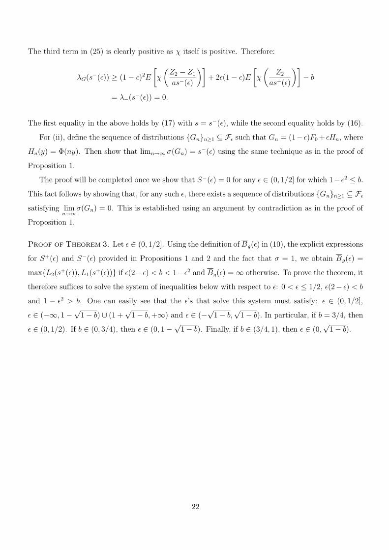
Proof of Theorem 3. Let ε ∈ (0, 1/2]. Using the definition ofBg(ε) in (10), the explicit expressions

for S+(ε) and S−(ε) provided in Propositions 1 and 2 and the fact that σ = 1, we obtain Bg(ε) =

max{L2(s+(ε)), L1(s

+(ε))} if ε(2−ε) < b < 1−ε2 and Bg(ε) =∞ otherwise. To prove the theorem, it

therefore suffices to solve the system of inequalities below with respect to ε: 0 < ε ≤ 1/2, ε(2− ε) < b

and 1 − ε2 > b. One can easily see that the ε’s that solve this system must satisfy: ε ∈ (0, 1/2],

ε ∈ (−∞, 1−√1− b) ∪ (1 +

√1− b,+∞) and ε ∈ (−

√1− b,

√1− b). In particular, if b = 3/4, then

ε ∈ (0, 1/2). If b ∈ (0, 3/4), then ε ∈ (0, 1−√1− b). Finally, if b ∈ (3/4, 1), then ε ∈ (0,

√1− b).

22

Figures and Tables.

0 0.5 1 1.5 2 2.5 3 3.5 40

0.5

1

1.5

2

2.5

3

3.5

4

4.5

5

s

L1(s) = −ln(s)

L2(s) = ln(s)

S−(ε)/σ0 S+(ε)/σ

0

Figure 1: Plot of the functions L1(s) = − ln(s), 0 < s ≤ 1, and L2(s) = ln(s), s ≥ 1. For the situationdepicted here, the maxbias is Bg(ε) = − ln(S−(ε)/σ).

23

0.0 0.2 0.4 0.6 0.8 1.0

−20

−10

010

20

ε = 0

x

y

0.0 0.2 0.4 0.6 0.8 1.0

−20

−10

010

20

ε = 0.05

x

y

0.0 0.2 0.4 0.6 0.8 1.0

−20

−10

010

20

ε = 0.10

xy

0.0 0.2 0.4 0.6 0.8 1.0

−20

−10

010

20

ε = 0.20

x

y

0.0 0.2 0.4 0.6 0.8 1.0

−20

−10

010

20

ε = 0.30

x

y

0.0 0.2 0.4 0.6 0.8 1.0

−20

−10

010

20ε = 0.40

x

y

Figure 2: Data simulated from model (1) for the simulation settings with n = 100 and H(y) = Φ(y/10).

The six panels show data corresponding to different amounts of contamination. The true regression function

is superimposed.

24

0.0 0.2 0.4 0.6 0.8 1.0

−10

−50

510

15

ε = 0

x

y

0.0 0.2 0.4 0.6 0.8 1.0

−10

−50

510

15

ε = 0.05

x

y

0.0 0.2 0.4 0.6 0.8 1.0

−10

−50

510

15

ε = 0.10

xy

0.0 0.2 0.4 0.6 0.8 1.0

−10

−50

510

15

ε = 0.20

x

y

0.0 0.2 0.4 0.6 0.8 1.0

−10

−50

510

15

ε = 0.30

x

y

0.0 0.2 0.4 0.6 0.8 1.0

−10

−50

510

15ε = 0.40

x

y

Figure 3: Data simulated from model (1) for the simulation settings with n = 100 and H(y) = Φ(y − 10).The six panels show data corresponding to different amounts of contamination. The true regression curve is

superimposed.

25

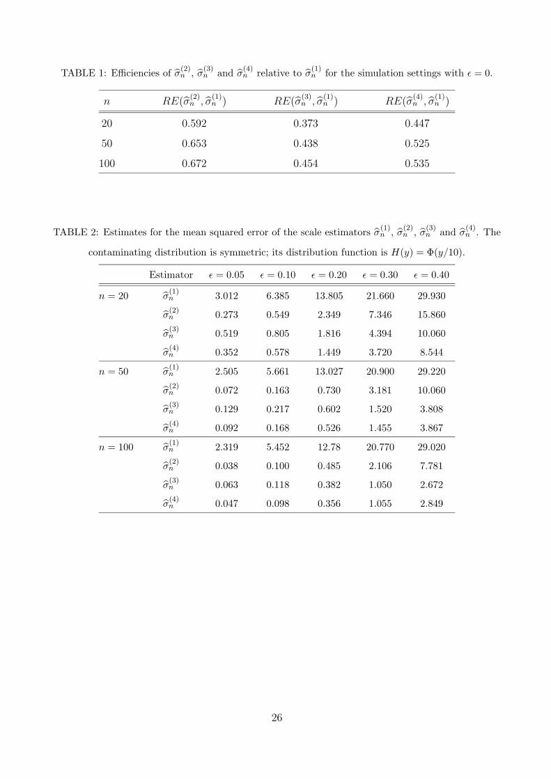
TABLE 1: Efficiencies of σ(2)n , σ

(3)n and σ

(4)n relative to σ

(1)n for the simulation settings with ε = 0.

n RE(σ(2)n , σ

(1)n ) RE(σ

(3)n , σ

(1)n ) RE(σ

(4)n , σ

(1)n )

20 0.592 0.373 0.447

50 0.653 0.438 0.525

100 0.672 0.454 0.535

TABLE 2: Estimates for the mean squared error of the scale estimators σ(1)n , σ

(2)n , σ

(3)n and σ

(4)n . The

contaminating distribution is symmetric; its distribution function is H(y) = Φ(y/10).

Estimator ε = 0.05 ε = 0.10 ε = 0.20 ε = 0.30 ε = 0.40

n = 20 σ(1)n 3.012 6.385 13.805 21.660 29.930

σ(2)n 0.273 0.549 2.349 7.346 15.860

σ(3)n 0.519 0.805 1.816 4.394 10.060

σ(4)n 0.352 0.578 1.449 3.720 8.544

n = 50 σ(1)n 2.505 5.661 13.027 20.900 29.220

σ(2)n 0.072 0.163 0.730 3.181 10.060

σ(3)n 0.129 0.217 0.602 1.520 3.808

σ(4)n 0.092 0.168 0.526 1.455 3.867

n = 100 σ(1)n 2.319 5.452 12.78 20.770 29.020

σ(2)n 0.038 0.100 0.485 2.106 7.781

σ(3)n 0.063 0.118 0.382 1.050 2.672

σ(4)n 0.047 0.098 0.356 1.055 2.849

26

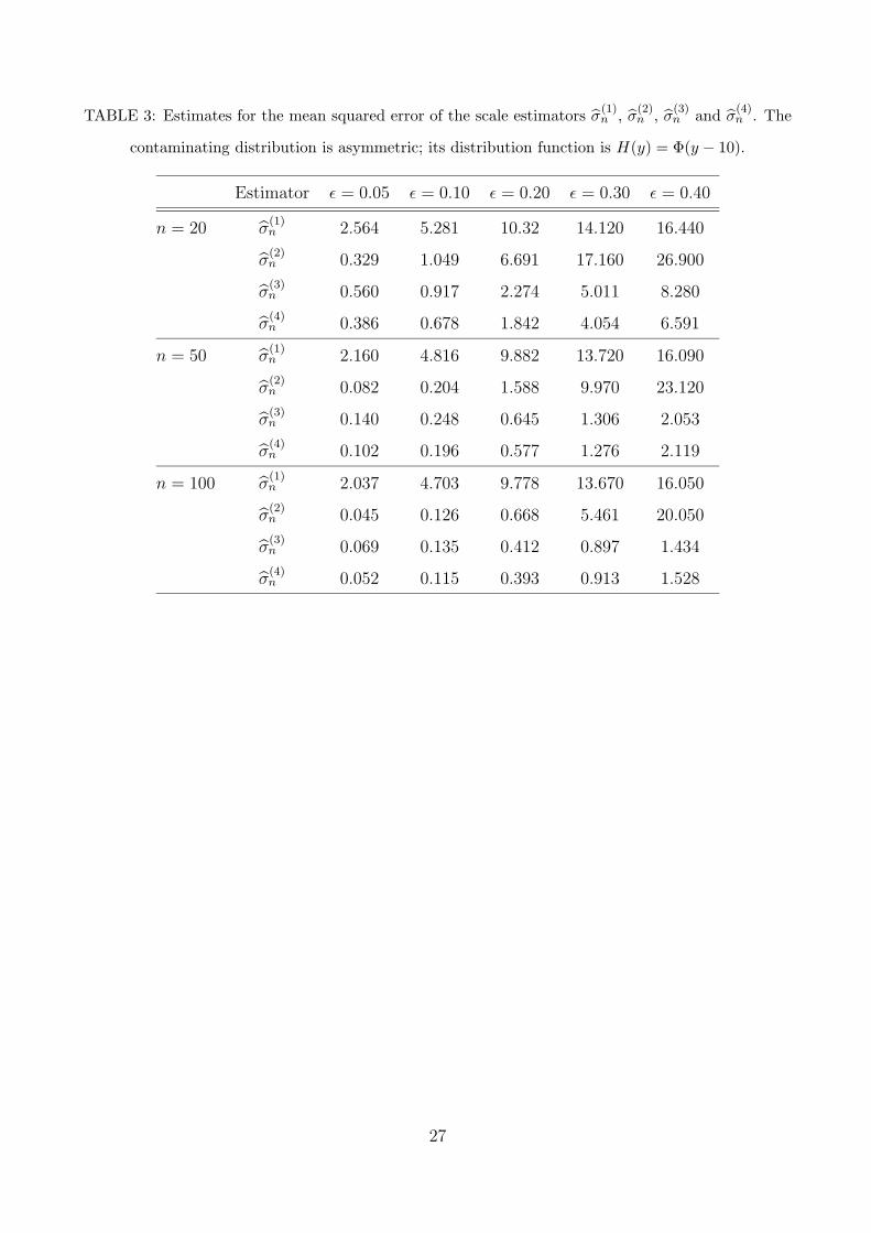
TABLE 3: Estimates for the mean squared error of the scale estimators σ(1)n , σ

(2)n , σ

(3)n and σ

(4)n . The

contaminating distribution is asymmetric; its distribution function is H(y) = Φ(y − 10).

Estimator ε = 0.05 ε = 0.10 ε = 0.20 ε = 0.30 ε = 0.40

n = 20 σ(1)n 2.564 5.281 10.32 14.120 16.440

σ(2)n 0.329 1.049 6.691 17.160 26.900

σ(3)n 0.560 0.917 2.274 5.011 8.280

σ(4)n 0.386 0.678 1.842 4.054 6.591

n = 50 σ(1)n 2.160 4.816 9.882 13.720 16.090

σ(2)n 0.082 0.204 1.588 9.970 23.120

σ(3)n 0.140 0.248 0.645 1.306 2.053

σ(4)n 0.102 0.196 0.577 1.276 2.119

n = 100 σ(1)n 2.037 4.703 9.778 13.670 16.050

σ(2)n 0.045 0.126 0.668 5.461 20.050

σ(3)n 0.069 0.135 0.412 0.897 1.434

σ(4)n 0.052 0.115 0.393 0.913 1.528

27

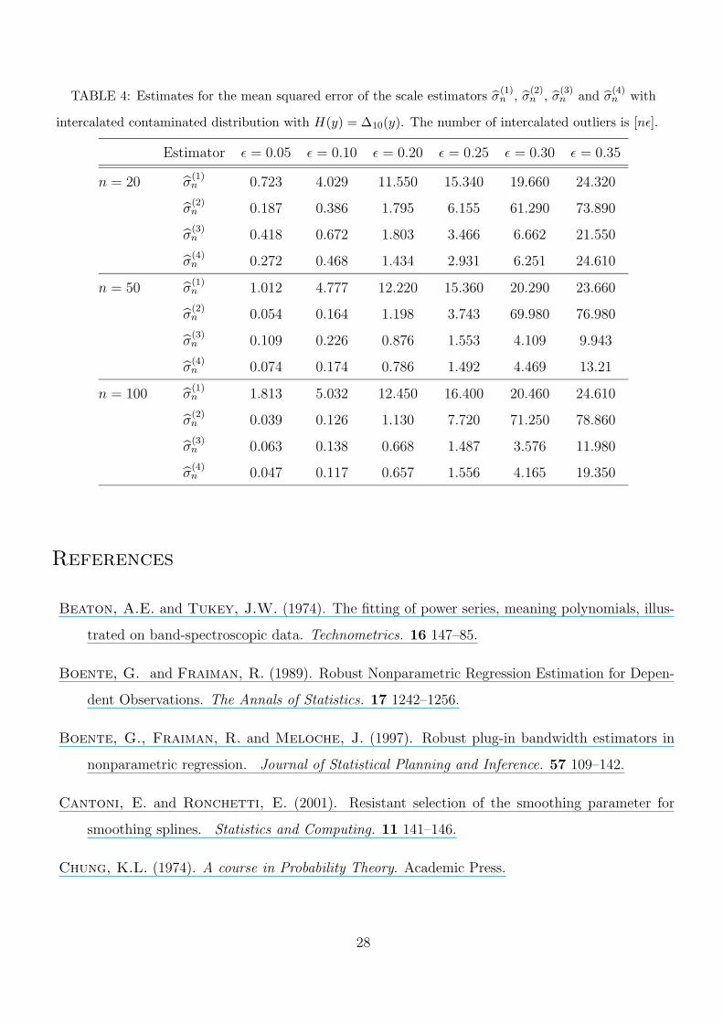
TABLE 4: Estimates for the mean squared error of the scale estimators σ(1)n , σ

(2)n , σ

(3)n and σ

(4)n with

intercalated contaminated distribution with H(y) = ∆10(y). The number of intercalated outliers is [nε].

Estimator ε = 0.05 ε = 0.10 ε = 0.20 ε = 0.25 ε = 0.30 ε = 0.35

n = 20 σ(1)n 0.723 4.029 11.550 15.340 19.660 24.320

σ(2)n 0.187 0.386 1.795 6.155 61.290 73.890

σ(3)n 0.418 0.672 1.803 3.466 6.662 21.550

σ(4)n 0.272 0.468 1.434 2.931 6.251 24.610

n = 50 σ(1)n 1.012 4.777 12.220 15.360 20.290 23.660

σ(2)n 0.054 0.164 1.198 3.743 69.980 76.980

σ(3)n 0.109 0.226 0.876 1.553 4.109 9.943

σ(4)n 0.074 0.174 0.786 1.492 4.469 13.21

n = 100 σ(1)n 1.813 5.032 12.450 16.400 20.460 24.610

σ(2)n 0.039 0.126 1.130 7.720 71.250 78.860

σ(3)n 0.063 0.138 0.668 1.487 3.576 11.980

σ(4)n 0.047 0.117 0.657 1.556 4.165 19.350

References

Beaton, A.E. and Tukey, J.W. (1974). The fitting of power series, meaning polynomials, illus-

trated on band-spectroscopic data. Technometrics. 16 147–85.

Boente, G. and Fraiman, R. (1989). Robust Nonparametric Regression Estimation for Depen-

dent Observations. The Annals of Statistics. 17 1242–1256.

Boente, G., Fraiman, R. and Meloche, J. (1997). Robust plug-in bandwidth estimators in

nonparametric regression. Journal of Statistical Planning and Inference. 57 109–142.

Cantoni, E. and Ronchetti, E. (2001). Resistant selection of the smoothing parameter for

smoothing splines. Statistics and Computing. 11 141–146.

Chung, K.L. (1974). A course in Probability Theory. Academic Press.

28

Dette, H., Munk, A. and Wagner, T. (1998). Estimating the variance in nonparametric

regression - What is a reasonable choice? Journal of the Royal Statistics Society. 60 751–764.

Ghement, I., Ruiz, M. and Zamar, R. (2006). Robust Estimation of Error Scale in Nonpara-

metric Regression Models. Technical Report # 218. Department of Statistics, University of

British Columbia.

Hannig, J. and Lee, T.C.M. (2006). Robust SiZer for Exploration of Regression Structures and

Outlier Detection. Journal of Computational and Graphical Statistics. 15 101–117.

Hardle, W. and Gasser, T. (1984). Robust nonparametric function fitting. Journal of the

Royal Statistical Society, Series B. 46 42–51.

Hardle, W. and Tsybakov, A. B. (1988). Robust Nonparametric Regression with Simultaneous

Scale Curve Estimation. The Annals of Statistics. 16 120–135.

Leung, D.H.-Y. (2005). Cross-validation in nonparametric regression with outliers. Journal of

Nonparametric Statistics. 2 333–339.

Leung, D.H.-Y., Marriott, F.H.C. and Wu, E.K.H. (1993). Bandwidth selection in robust

smoothing. Journal of Nonparametric Statistics. 2 333–339.

Rice, J. (1984). Bandwidth Choice for Nonparametric Regression. The Annals of Statistics. 12

1215–1230.

29