Robust estimation in the errors variables model via weighted likelihood estimating equations

Test (1997) Vol. ~, No. 1, pp. 187-203

187

Robust Estimation in the Errors Variables Model via Weighted

Likelihood Estimating Equations A. B A S U and S. S A R K A R

Applied Statistics Unit, h~dian Statistical Instintte, 203 B.T. Road, Calcutta 700 035, hulia

Deparonent of Statistics, Oklahoma State University, Stillwatet; OK 74078, USA

SUMMARY

Parameters estimates for the errors-in-variables model are obtained by solv- ing weighted likelihood estimating equations. They are consistent, asymp- totically normal and asymptotically fully efficient, and exhibit robustness properties similar to the minimum disparity estimators (Basu and Sarkar 1994a) but are immensely simpler to compute and have some theoretical advantages over the latter. We illustrate the robustness properties through some numerical studies similar to those of Zamar (1989).

Keywords: MEASUREMENT ERROR MODEl.; DISPARITY: HELLINGER

DISTANCE; ROBUSTNESS: WEIGIITED LIKELIHOOD ESTIMATOR.

1. INTRODUCTION

Consider the classical errors-in-variables model:

/ x y~ = ~ i, Yi = yi + ei, X i = x i + u~, (1)

fo r i = 1 , . . . , n , w h e r e / 3 = ( / 3 1 , . . . , f3p)', Yi and x~ deno te the true

va lues o f the var iab les obse rved as ]'~ and X i = ( X j i , X 2 i , . , -Xpi) I

Received March 1995; Revised January 1997.

188 A. Basu and S. Sarkar

containing measurement errors ei and ui = (~qi, u2i , . . . , "U, pi) t respec- tively, and {xi } and {6i = (ei, ul) ' } are independent sequences of i.i.d. random vectors such that x~ ,-~ Np[lZx, Exz] and ei ~ N[0, ~c~]. The common distribution of the vectors (~, XI) is a multivariate normal dis- tribution. To make model (1) identifiable, we assume Ec~ is known up to a multiple (see Fuller 1987, Sec 2.3.2). The literature on robust estima- tion in errors-in-variables models is fairly small. It includes the works of Brown (1982), Zamar (1989), Cheng and Van Ness (1990, 1992) and Croos and Fuller (1991) on the classical model. Brown studied the iteratively reweighted orthogonal regression and Zamar investigated robust orthogonal regression M-estimators. Cheng and Van Ness ex- amined the classical and generalized M-estimators. Carroll and Gallo (1982) discussed the classical independent error model with replication of the predictors. Carroll, Eltinge and Ruppert (1993) studied the case where there are replicates of the observed predictors and the errors in the response and predictor variables are correlated.

Basu and Sarkar (1994a), hereafter referred to as B&S, considered minimum disparity estimators (MDEs), defined in Section 2, of the pa- rameters of model (1). Unlike the robust estimators previously studied for this model, the MDEs have been observed to exhibit strong robust- ness properties while at the same time havingfidl asymptotic efficiency at the model if the kernel can be chosen appropriately relative to the model. Such kernels are known as transparent kernels (Basu and Lindsay 1994). In a modest Monte Carlo study reported in B&S the minimum Hellinger distance estimator performed better than the orthogonal regression M- estimator of Zamar (1989) with contaminated data for model (1).

While the MDEs have several attractive properties, their asymptotic efficiency depends on the choice of transparent kernels which may not be available if the model distribution is not normal. In addition, the evaluation of the MDEs requires an enormous amount of computation. In this paper, following the approach of Basu, Markatou and Lindsay (1993) we consider weighted likelihood estimators (WLEs), defined in Section 2, which remove the above mentioned limitations of the MDEs. The disparity based WLEs are related to the MDEs and have similar efficiency and robustness properties but are far more practical in terms of the computational ease. In some numerical studies similar to those of Zamar (1989), the Hellinger distance based WLE appears to be competi-

Robust estimation in measurement error models 189

tive to the minimum Hellinger distance estimator in te~xns of robustness; in a Monte Carlo study of B&S, the latter was seen to outperform the orthogonal regression M-estimator of Zamar (1989). We emphasize, however, that the purpose of this paper is not to find just another ro- bust estimator; the proposed WLEs, like the MDEs, also achieve full asymptotic efficiency at the model.

The remainder of the paper is organized as follows. We discuss the MDEs and the WLEs in Section 2. Application of the weighted likelihood estimation to model (1) is discussed in Section 3. Section 4 presents results of a simulation study showing robustness of the Hellinger distance based WLE under an errors-in-variables model with nonnormal error distributions. In Section 5 we demonstrate the performance of the Hellinger distance based WLE through a real dataset; and in addition, we illustrate the computation of the Hellinger distance based WLE for a trivariate real dataset with two (non-intercept) explanatory variables.

2. MINIMUM DISPARITY AND WEIGHTED LIKELIHOOD ESTIMATION

2.1. Minimum. Disparity Estimation

B&S have reviewed minimum disparity estimation (Lindsay 1994; Basu and Lindsay 1994; Basu and Sarkar 1994b) for a family of continu- ous models rr~/~(-), indexed by/3 E IR p. Let g l , Z 2 , . . . , Z++ be k- dimensional i.i.d, observation vectors from ~rz,~(z). Minimum disparity estimators are obtained by minimizing disparities PG (f*, ~7~,}) which are density based distances with the special structure

= i i where ,f* (z) is a nonparametric kernel density estimator, 'm,~(z) is the model density smoothed with the same smooth kernel function and G is a real valued thrice differentiable convex function with G(0) = 0. Also ~*(z) = [(Tn, i~(z))- l f * ( z ) - 1] which is called the Pearson residual at z by Lindsay (1994). The squared Hellinger distance corresponds to G(m) --- [(m + 1) 1/2 - 1] 2. The minimizer of the likelihood disparity which corresponds to G(x) = (a: + 1) loge (,z' + 1) is called the "MLE*".

190 A. Basu and S. Sarkar

The estimating equation of the MLE* is

.[./ f :*(z) o , .. O m (x)dz

0 , 1 -~m~(x)( tz = O.

(2)

If the kernel chosen is transparent (see Basu and Lindsay 1994 and B&S), then MLE* is equal to the usual maximum likelihood estimator

Computation of the MDE requires iterative techniques including nu- merical evaluation of integrals. For multivariate observations this entails numerical evaluation of multiple integrals. Computation becomes more and more time consuming as k, the dimension of the observation vectors, grows. We next describe a modification of the above estimation method which avoids this problem without sacrificing efficiency or robustness properties. More details of this modification are given in Basu, Markatou and Lindsay (1993).

2.2. Weighted Likelihood Estimator

The minimum disparity estimating equations can be expressed as

o~Pc, = . . . . A(&(z)) mS(z ) dz = O, (3)

where A(x) = (1 + x ) [ ~ G ( x ) ] - G(x). The function A(x) is the residual adjustment function con'esponding to a disparity G. Usually, A(x) is redefined such that A(0) = 0 and dA(:r)]:r,=O = 1. This means for the Hellinger distance A(x) = 2[(x + 1) 1/2 - 1]. Most of the theoretical properties of the MDE is governed by the form of the residual adjustment function. For disparities like the Hellinger distance the residual adjustment function can strongly downweight observations

d2 At with large Pearson residuals. The quantity A2 = d.-~. ~x/[ .~=0 can be used as a descriptor of the robustness of the MDE; large negative values of A2 lead to greater robustness. For the Hellinger distance A2 = - 1/2, and but for the likelihood disparity A2 = 0 See Basu and Lindsay (1994) for more details.

Robttst estimation in measurement error models "191

Tim estimating equation (3) can be rewritten as

[ A(6 ~) + 1.] + . / . . . / [ - ~ - + ~ (6* 1) [ ff-~,n)!~(z)] dz

o �9

. . . . L ",---YJ

(4)

where F* is the distribution function corresponding to f* and w(x) =

(x+ 1)-~[A(x)+ 1] withw(0) = 1, ~w(x)l:r,=0 = 0and ~w(x) la :=0 = A2. But equation (4) is a weighted version of the estimating equations of the MLE* in equation (2) with weights w(.). In analogy to equation (4) one can define the following estimating equation for 13

i.e.,

where

,,-~ ~ w(~*(z~)),,(z,, 13) = 0 (5) i =1

c 9 u(z,~) = ~ log~ m~(z)

is the usual maximum likelihood score function and F,~ is the empirical distribution function. Note that the kernel smoothing is now o1@ in the weight part and not in the score part of the above equation. Just as one does in iteratively reweighted least squares estimation method (Beaton and Tukey 1974; Holland and Welsch 1977; Birch 1980), equation (5) can be solved iteratively by updating the weights w (.) at every stage. The solution/~ of the above estimating equation is called the WLE, which depends on the choice of disparity G.

By the results of Basu, Markatou and Lindsay (1993), the WLEs are asymptotically tully efficient at the model. Under the model, asymptot- ically the weights w(& (Zi)) tend to one and equation (5) behaves like the maximum likelihood score equation for all the disparities. In addi- tion, WLEs generated by disparities like the Hellinger distance may have

"199 A. Basu and S. Sarkar

good robustness properties since the weight function w(.) downweights observations with large Pearson residuals. Unlike the MDEs, the WLEs do not require a transparent kernel to achieve full asymptotic efficiency,

2.3. A Root Selection Criterion under Multiple Roots

Like the quasi likelihood estimates (Wedderburn 1974) the weighted likelihood estimates are obtained as roots of a set of estimating equations and the computation is not based on any specilic optimization criterion. Any nonlinear equation can potentially have more than one root. While computing the MLE by solving the ordinary likelihood equations, the multiple roots problem can be resolved by considering the root at which the likelihood function is maximized. This approach is not possible with the weighted likelihood estimation method when equation (5) has multiple roots.

However, since the estimating equation (5) is obtained by simply replacing the smoothed model and smoothed empiricals in equation (4) with the corresponding unsmoothed versions, one approach to root selec- tion may be to compare the roots against the parallel disparity measure whose minimizer is obtained as a solution of equation (4). While it can not be guaranteed that this method will always solve the multiple roots problem, we expect that this will help us identify the good roots and reject the bad roots most of the time. To illustrate this, consider m~ to be N(/L 1) model, kernel function to be N(0: h 2) with h = 0.5, observed empirical distribution F,,(z) to be the mixture distribution [0.SN(0, 1) + 0.5N(10, 1)] and the disparity to be the Hellinger dis- tance. Then, 7t~/~ is N(/L 1 + h "2) and the kernel density estimator f* is

the [0.SN(0, 1 + h 2) + 0.SN(10, 1 + h2)] density. In this case, using the Hellinger distance based weights three roots for the estimating equation (5), i.e., for f w(b*)[Om,~/Ofl]dF,~ (z) = 0, are observed --one close to 0, one close to 10 and one exactly at 5. An investigation of the Hellinger distance (parallel disparity measure) between f* and m~ as a function of fl reveals that the distance has one local maximum at 5, and two local minima - one close to 0 and one close to 10. Thus, the parallel disparity measure allows us to isolate the bad root of the estimating equation in this case.

Robust estimation in measurement error models 193

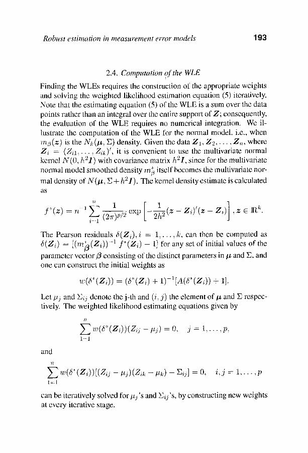
2.4. Comt~umtion of the WLE

Finding the WLEs requires the construction of the appropriate weights and solving the weighted likelihood estimation equation (5) iteratively. Note that the estimating equation (5) of the WLE is a sum over the data points rather than an integral over the entire support of Z; consequently, the evaluation of the WLE requires no numerical integration. We il- lustrate the computation of the WLE for the normal model, i.e., when m;3(z) is the N~(/z, E) density. Given the data Z1, Z2 . . . . , Z,,, where Z i = (Z,:I , . . . , Z,i~) ~, it is convenient to use the multivariate normal kernel N(0, h'2I) with covariance matrix h2I, since for the multivariate normal model smoothed density m)~ itself becomes the multivariate nor-

mal density of N(/z, E + h2I). The kernel density estimate is calculated a s

' [ ] f,(~) = n_l ~ 1 1 = (27r)p/2 exp - 9 - ~ ( z Z i ) ' ( z - Zi) , z E ]Rk.

The Pearson residuals 6(Zi), i = 1 , . . . , k, can then be computed as 6(Zi) = [(m~(Zi)) -1 f*(Zi) - 1 t to," any set of initial values of the

parameter vector/3 consisting of the distinct parameters in/~ and E, and one can construct the initial weights as

w(6*(Zi)) -= (6*(Zi) + 1)-I[A(~5*(Zi)) + 1].

Let pj and Eij denote the j-th and (i, j ) the element of # and E respec- tively. The weighted likelihood estimating equations given by

y ~ , w ( 6 * ( z ~ ) ) ( z ~ - # 9 = o, j = 1 , . . . ,~ , 1=1

and

1l

Z w ( ~ * ( Z i ) ) [ ( Z i j - l z j ) ( Z i ~ : - # t ~ ) - Eij]=O, i , j = 1 , . . . , p 1=1

can be iteratively solved for #j ' s and ~ij 'S, by constructing new weights at every iterative stage.

"194 A. Basu and S. Sarkar

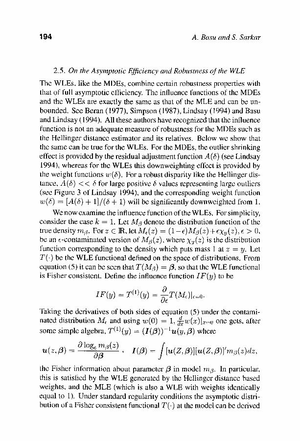
2.5. On the Asymptotic Efficiency and Robusmess of the WLE

The WLEs, like the MDEs, combine certain robustness properties with that of full asymptotic efficiency. The influence functions of the MDEs and the WLEs are exactly the same as that of the MLE and can be un- bounded. See Beran (1977), Simpson (1987), Lindsay (1994) and Basu and Lindsay (1994). All these authors have recognized that the influence function is not an adequate measure of robustness for the MDEs such as the Hellinger distance estimator and its relatives. Below we show that the same can be true for the WLEs. For the MDEs, the outlier shrinking effect is provided by the residual adjustment function A(~) (see Lindsay 1994), whereas for the WLEs this downweighting effect is provided by the weight functions w(6). For a robust disparity like tile Heilinger dis- tance, A(5) < < 5 for large positive 5 values representing large outliers (see Figure 3 of Lindsay 1994), and the corresponding weight function w(~5) = [A(3) + 1]/(6 + 1) will be significantly downweighted from 1.

We now examine the influence function of the WLEs. For simplicity, consider the case k = 1. Let ~I/3 denote the distribution function of the true density m,q. For z C IR, let M~(z) = (1 -e)~,I;3(z) +eXy(Z), e > O, be an e-contaminated version of 3/i/~(z), where Xu(z) is the distribution function corresponding to the density which puts mass 1 at z = y. Let T(-) be the WLE functional defined on the space of distributions. From equation (5) it can be seen that T(Mt~ ) =/3 , so that the WLE functional is Fisher consistent. Define the influence ftmction IF(y) to be

I f ( y ) = T(l)(y) : O r ( M , ) l , = 0 .

Taking the derivatives of both sides of equation (5) under the contami- d l l z \ hated distribution -Me and using w(0) = 1, ~ '~ (x)lz=0 one gets, after

some simple algebra, T(1)(y) = (I(/3))-lu(y,/3) where

u(z,/3) = O l~ rn~(z) f ) 0/3 , i t ( /3)=, [u(z,/3

the Fisher information about parameter/3 in model m:~. In particular, this is satisfied by the WLE generated by the Hellinger distance based weights, and the MLE (which is also a WLE with weights identically equal to 1). Under standard regularity conditions the asymptotic distri- bution of a Fisher consistent functional T(-) at the model can be derived

Robust estimation in measurement ertvr models "195

using the expression

'~,~/2(T(F,J - / 3 ) = 'n.--~EL,/F(Z0 + Op(1),

with F,~ denoting the empirical distribution function. See, for example, Femholz (1983). This implies that the asymptotic distribution of the WLEs and the MLE am the same, indicating the full asymptotic effi- ciency of the WLEs and the potential of their influence function to be unbounded.

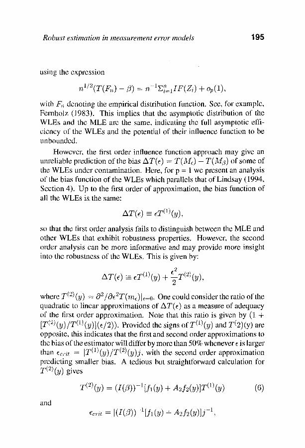
Howevm; the first order influence function approach may give an unreliable prediction of the bias AT(e) = T(M~) - T(M;3) of some of the WLEs under contamination. Hem, for p = 1 we present an analysis of the bias function of the WLEs which parallels that of Lindsay (1994, Section 4). Up to the first order of approximation, tile bias function of all the WLEs is, the same:

AT(e) = eTO)(y),

so that the first order analysis fails to distinguish between the MLE and other WLEs that exhibit robustness properties. However, the second order analysis can be more informative and may provide more insight into the robustness of the WLEs. This is given by:

~2 .

- TO)(V) +

where T (2) (y) = O2/Oe'2T(me)]e=0. One could consider the ratio of the quadratic to linear approximations of AT(e) as a measure of adequacy of the first order approximation. Note that this ratio is given by (1 + [T(2)(y)/TO)(y)](e/2)). Provided the signs of T(1)(y) and T(2)(y) are opposite, this indicates that the first and second order approximations to the bias of the estimator will differ by more than 50% whenever e is larger than ec,.it = IT (I)(y)/T (2)(y)j, with the second order approximation predicting smaller bias. A tedious but straightlbrward calculation for T (~) (y) gives

T(2)(y) = ( I ( /3) ) - l [ f l (y) + A2,f.2(y)]T(~)(y) (6)

and ee.rit = 1(I(/3))-l[f l(y) + A2f2(y)]j -1,

196 A. Basu andS. Sarl,'ar

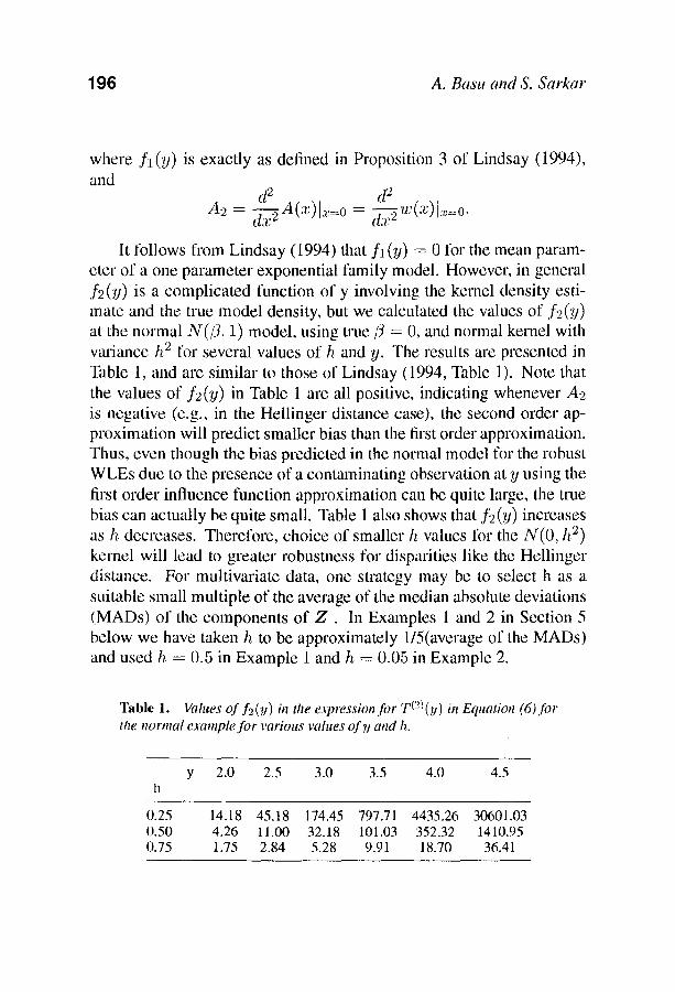
where f l ( Y ) is exactly as defined in Proposition 3 o:f Lindsay (1994), and

d 2 d 2 , A2 = ~ A ( z ) l x = o = ~ ,~(z) lx=;o .

It follows fi'om Lindsay (1994) that f l (Y) = 0 for the mean param- eter of a one parameter exponential family model. However, in general .f2 (9) is a complicated function of y involving the kernel density esti- mate and the true model density, but we calculated the values of f2(Y) at the normal N ( / L 1) model, using true/3 = O, and normal kernel with variance h 2 for several values of h and y. The results are presented in Table 1, and are similar to those of Lindsay (1994, Table 1). Note that the values of f2(y) in Table 1 are all positive, indicating whenever A2 is negative (e.g., in the Hellinger distance case), the second order ap- proximation will predict smaller bias than the first order approximation. Thus, even though the bias predicted in the normal model for the robust WLEs due to the presence of a contaminating observation at y using the first order influence function approximation can be quite large, the true bias can actually be quite small. Table 1 also shows that f2(Y) increases as h decreases. Therefore, choice of smaller h values for the N(0, h 2) kernel will lead to greater robustness for disparities like the Hellinger distance. For multivariate data, one strategy may be to select h as a suitable small multiple of the average of the median absolute deviations (MADs) of the components of Z . In Examples 1 and 2 in Section 5 below we have taken h to be approximately l/5(average of the MADs) and used h = 0.5 in Example 1 and h, = 0.05 in Example 2.

Table 1. Values of f.~(y) in the e,~pression for T(~)(~v) in Equation (6) Jor the norntal exantple for valTous vahtes of y and h,.

y 2.0 2.5 3.0 3.5 4.0 4.5 h

0.25 14.18 45.18 174.45 797.71 4435.26 30601.03 0.50 4,26 11.00 32.18 101.03 352.32 1410.95 0.75 1.75 2.84 5.28 9.91 18.70 36.41

Robust estimation in measurement error models 197

3. WEIGHTED LIKELIHOOD ESTIMATION IN THE ERRORS-IN-VARIABLES MODEL

Since in model (1) the joint distribution of Zi = (~, X~i) ~ is multivariate normal, the model parameters can be determined by a straightforward application of the weighted likelihood estimation method considered in Section 2.4. Here ~r~i~(z) is the Np+t(/.r ~) density. In the weighted likelihood estimation procedure any smooth kernel can be used to obtain a nonparalnetric density estimator and to smooth the model density. In particular, if the Np+l(O, h2I) density is used as the kernel, where I is the (p + 1) x (p + 1) identity matrix, then the smoothed model density m i} (z) would be the Np+l (lz, ~ + h2I) density. Then, given a particular disparity Pc;, the corresponding WLE of the parameter vector can be calculated by iteratively solving equation (5). From the viewpoint of robustness some disparity measures are more desirable than others. In our study we have investigated the WLE with weights based on the Hellinger distance (with A(x) = 2[(.~: + 1) ~/2 - 1]) and the results are presented in Sections 4 and 5. In computing the WLEs, unlike the MDEs, we no longer have to choose a transparent kernel and any other smooth kernel would work as well.

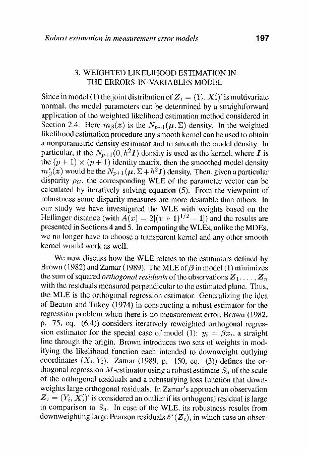
We now discuss how the WLE relates to the estimators defined by Brown (1.982) and Zamar (1989). The MLE of et in model (1) minimizes the sum of squared orthogonal residuals o17 the observations Z1 . . . . , Z~, with the residuals measured perpendicular to the estimated plane. Thus, the MLE is the orthogonal regression estimator: Generalizing the idea of Beaton and Tukey (1974) in constructing a robust estimator for the regression problem when there is no measurement error, Brown (1982, p. 75, eq. (6.4)) considers iteratively reweighted orthogonal regres- sion estimator for the special case of model (1): Yi = /3xi, a straight line through the origin. Brown introduces two sets of weights in mod- ifying the likelihood function each intended to downweight outlying coordinates (X,i, Y/). Zamar (1989, p. 150, eq. (3)) defines the or- thogonal regression M-estimator using a robust estimate S,,. of the scale of the orthogonal residuals and a robustifying loss function that down- weights large orthogonal residuals. In Zamar's approach an observation Zi = (~, X~i) ~ is considered an outlier if its orthogonal residual is large in comparison to 5',~. In case of the WLE, its robustness results from downweighting large Pearson residuals ~5" (Zi), in which case an obser-

198 A. Basu and S. Sarkar

vation Z,: is considered an outlier if the kernel density f * ( Z i ) at Z i is large relative to the smoothed model density m~3(Zi ) at Zi . Thus, the WLE downweighks observations which represent large residuals in a probabilistic, rather than geometric, sense.

4. SIMULATION RESULTS

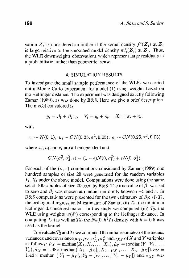
To investigate the small sample performance of the WLEs we carried out a Monte Carlo experiment for model (1) using weights based on the Hellinger distance. The experiment was designed exactly lbllowing Zamar (1989), as was done by B&S. Here we give a brief description. The model considered is

Yi = ~1 Jr- t~2Xi, Yi = yi + ei, X i = :ri + ui,

with

xi "-' N(O, 1), ui "." CN(0.25, a2; 0.05), ei "~ CN(0.25, v 2, 0.05)

where xi , ui and ei am all independent and

CN(a~2, ~7.~, e ) = (1- e.)X(0, a ~ ) + eN(O,a~) .

For each of the (or, ~-) combinations considered by Zamar (1989) one hundred samples of size 20 were generated for the random variables Y~, Xi under the above model. Computations were done using the same set of 100 samples of size 20 used by B&S. The true value of/31 was set to zero and 32 was chosen at random unilbrmly between - 5 and 5. In B&S computations were presented lbr the two estimators of [32: (i) Tl, the orthogonal regression M-estimator of Zamar; (ii) T2, the minimum Hellinger distance estimator. In this study we computed (iii) T3, the WLE using weights w(6*) colxesponding to the Hellinger distance. In computing Ta (as well as T.2) the N2(0, h2I) density with h = 0.5 was used as the kernel.

To evaluate T2 and T3 we computed the initial estimates of the means, variances and covariance P x , PY, cri{~, cry- and a x y of X and Y variables as lbllows: fix = median(X1, X 2 , . . . , X~z),/~y = median(~q, Y2,. �9 �9 )~), &x = 1.48x m e d i a n ( l X l - [ ~ x ] , IX .2-[ tx[ , . . . , ] X ~ - [ t x ] ) , &y = 1.48• median (IY1 - [ty[, IY2 - fi, YI , . . . , [Y~ - [ty[) and 5 x y was

Robust estimation in meastuement error models 199

computed using the covariance estimate formula as given in equation (2.7) of Huber (1981, p. 203).

The criterion m defined in equation (6) of Zamar (1989) and used by B&S is applied here to measure the performance of the WLE. For the i-th estimator T/, it is detined by

100 [ 11 + Tij/32jl ]

j = l

where E i and/39~j are respectively the i-th estimator and the true value of [32 for the j-th replication. An estimator is better than another if its value for measure m is smallel:

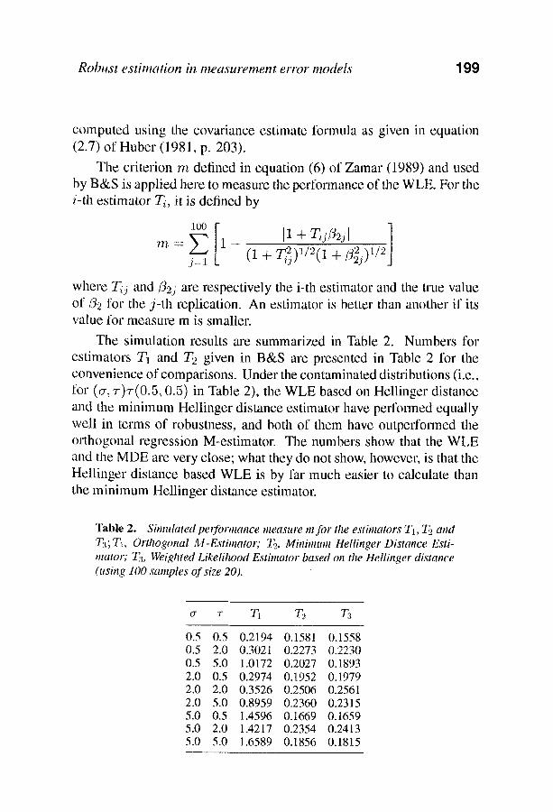
The simulation results am summarized in Table 2. Numbers for estimators TL and T2 given in B&S are presented in Table 2 for the convenience of comparisons. Under the contaminated distributions (i.e., for (c~, r)r(0.5, 0.5) in Table 2), the WLE based on Hellinger distance and the minimum Hellinger distance estimator have performed equally well in terms of robustness, and both of them have outperformed the orthogonal regression M-estimator. The numbers show that the WLE and the MDE are very close; what they do not show, however; is that the Hellinger distance based WLE is by far much easier to calculate than the minimum Hellinger distance estimator.

Table 2. Simulated pelformance nteasure m for the estimatol:~ T~, ~ and 7~; Tb Orthogonal M-Estimator; 73, Minintunt Hellinger Distance E~ti- mator; T..3, Weighted Likelihood Estimator based on the Hellinger distance (using 100 samples of size 20).

0.5 0.5 0.2194 0.1581 0.1558 0.5 2.0 0.302I 0.2273 0.2230 0.5 5.0 1.0172 0.2027 0.1893 2.0 0.5 0.2974 0.1952 0.1979 2.0 2.0 0.3526 0.2506 0.2561 2.0 5.0 0.8959 0.2360 0.2315 5.0 0.5 1.4596 0.1669 0.1659 5.0 2.0 1.4217 0.2354 0.2413 5.0 5.0 1.6589 0.1856 0.1815

200 A, Basu and S. Sarkar

5. APPLICATIONS

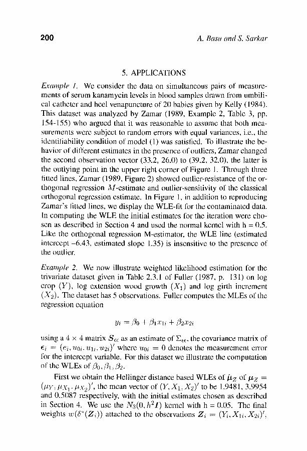
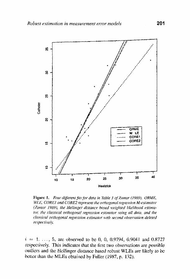
Example 1. We consider the data on simultaneous pairs of measure- ments of serum kanamycin levels in blood samples drawn fi'om umbili- cal catheter and heel venapuncture of 20 babies given by Kelly (1984). This dataset was analyzed by Zamar (1989, Example 2, Table 3, pp. 154-1155) who argued that it was reasonable to assume that both mea- surelnents were subject to random errors with equal variances, i.e., the identifiability condition of model (1) was satistied. To illustrate the be- havior of different estimates in the presence of outliers, Zamar changed the second observation vector (33.2, 26.0) to (39.2, 32.0), the latter is the outlying point in the upper right corner of Figure 1. Through throe fitted lines, Zamar (1989, Figure 2) showed outlier-resistance of the or- thogonal regression M-estimate and outlier-sensitivity of the classical orthogonal regression estimate. In Figure 1, in addition to reproducing Zamar's fitted lines, we display the WLE-fit for the contaminated data. In computing the WLE the initial estimates for the iteration were cho- sen as described in Section 4 and used the normal kernel with h = 0.5. Like the orthogonal regression M-estimator, the WLE line (estimated intercept -6.43, estimated slope 1.35) is insensitive to the presence of the outlier.

Eranq)le 2. We now illustrate weighted likelihood estimation for the tfivafiate dataset given in Table 2.3.1 of Fuller (1987, p. 131) on log crop (Y), log extension wood growth (X~) and log girth increment (X2). The dataset has 5 observations. Fuller computes the MLEs of the regression equation

yi =/30 +/31:rii +/3e:r.2i

using a 4 • 4 matrix S~ as an estimate of E~c, the covariance matrix of ~i = (ei, ~toi, 'ltli, "lt2i) ! where "uoi = 0 denotes the measurement error for the intercept variable. For this dataset we illustrate the computation of the WLEs of/3o,/31,/32.

First we obtain the Hellinger distance based WLEs of/2 z of ~z = (#Y: lz.\h, l ,x2) , the mean vector of ()L X~ X2) to be 1.9481, 3.9954 and 0.5(i)87 respectively, with the initial estimates chosen as described in Section 4. We use the N:3(0, h2I) kernel with h = 0.05. The final weights w( , (Zi)) attached to the observations Z~ (Yi, Xli , X2i) ~,

Robust estimation in measurement error models 201

I n r

l // ,p

r 1 f f

o a t

,

t%l . �9 �9

/i/ '" r - �9 �9

7

( ~ I ~

. / /'" . t

o ,

J t o

, ,

e p �9 , ~

o *

W COREI I

10 15 20 25

Heels~ck

30 35 40

Figure 1. Four different fits for data in Table 3 of Zamar (1989). ORML. WLE, CORE1 attd CORE2 represent the orthogonal regression M-estimator (Zamar 1989), ttte Hellinger distance based weigttted likelilzood estima- tor; the cta~,wical orthogonal regression estimator using all data. and the classical ortttogonal regression estimator with second observation deleted respective(~,.

'i = 1, . . . , 5, are observed to be 0, 0, 0.9794, 0.9041 and 0.8727 respectively. This indicates that the first two observations are possible outliers and the Hellinger distance based robttst WLEs are likely to be better than the MLEs obtained by Fuller (1987, p. 132).

902 A. B a s u a n d S. Sarl<ar

Next to compute robust estimates of/}1 and/~2 using the WLE of /z z we modify Fuller's method of MLE computation as described in Theorem 2.3.1 of Fuller (1987, p. 124). We calculate the 3 • 3 matrix

-1 t~

- i,z)(Z - i , z ) '

i=1

and find the smallest root of the detenninantal equation I M ~ z - ASCii = 0 where S'~ is the 3 • 3 submatrix of S~c obtained by removing the 2nd row and 2nd column of the latter. Let M~. x be the 2 • 2 lower submatrix of 1 V I ~ z , let S , , denote the 2 • _9 lower submatrix of S*~ and let S,,c denote the 2 x 1 vector obtained by deleting the first component of the first column of S~c. The smallest root ~ is found to be 2.982 x 10 -9. Then the Hellinger distance based WLEs of/31 and/32 obtained by using (/31~, f32)' ( M x x ~ S * w u , ) - l ( 1 V l : ~ , y " * = - �9 - ~S~,~,) are observed to be 0.0567 and 2.1801 respectively, and the Hellinger distance based WLE

,73o = f zy - f31f ix 1 - f3f ix9 of/30 is found to be 0.6125.

ACKNOWLEDGEMENTS

The research of the first author was partially supported by a Mathematics Department Research Award, University of Texas at Austin, while the author was a faculty member at the University of Texas. The research of the second author was supported in part by a Grant fi'om the College of Arts and Sciences at Oklahoma State University. The authors wish to thank Professor Bruce G. Lindsay for some helpful comments, a referee and the Associate Editor for many helpful suggestions that led to the present improved version of this paper.

REFERENCES

Basu, A. and Lindsay, B. G. (1994). Minimum disparily estimation for continuous models: Efficiency, distributions and robusmess. Ann. Inst. Statist. Math. 46, 683- 705.

Basu, A., Markatou, M. and Lindsay, B. G. (1993). likelihood estimating equations. Tech. Rep. 93-01, Department of Statistics, Columbia University, New York, NY.

Basu, A. and Sarkar, S. (1994a). Minimum disparity estimation in the errors-in- variables model. Statist. Probab. Lett. 20, 69-73:

R o b u s t e s t ima t ion in m e a s u r e m e n t error mode l s 9 0 3

Basu, A. and Sarkar, S. (1994b). The trade-off between robustness and efficiency and the effect of model smoothing in minimum disparity inference. J. Statist. Comput. Simul. 50, 173-185.

B eaton, A. E. and Tukey, J. W. (1974). The fitting o f power series, meaning polynomials, illustrated on band spectroscopic data. Technometrics 16, 1470-1485.

Birch, J. B. (1980). Some convergence properties of iterated least squares in the location model. Commun. Statist. B 9, 359-369.

Brown, M. (1982). Robust line estimation with errors m both variables. J. Amer. Statist. Assoc. 77, 71-79.

Carroll, R. and Gallo, R (1982). Some aspects of robustness in the functional errors in variables model. Commun. Statist. A 11, 2573-2585.

C~roll, R. J. and Eltinge, J. L. and Ruppert, D. (1993). Robust linear regression in replicated measurement error models. Statist. Probab. Lett. 16, 169-175.

Cheng, C. and J. W. Van Ness (1990). Bounded influence errors in variables regression, (R Brown and W. A. Fuller, eds.), Contemporary Mathematics: Statistical Analysis of Measurement Error Models and Applications (Amer. Math. Soc. Providence, RI).

Cheng, C. and J. W. Van Ness (1992). Generalized M-estimators for errors-in-variables regression. Ann. Statist. 20, 385-397.

Croos, J. and Fuller, W. A. (1991). Robust estimation in measurement error models. American Statistical Association 1991 Proceedings of the Business and Statistics Section, 283-288.

Fernholz, L.T. (1983). Von Mises Calculus for statistical Functionals. New York: Springer Verlag.

Fuller, W. A. (1987). Measurement error models. New York: Wiley Holland; R W. and Welsch, R. E. (1977). Robust regression using iteratively reweighted

least squares. Commun. Statist. A 6, 813-827. Huber, R J. (1981). Robust Statistics. New York: Wiley Kelly, G. (1984). The influence function in the errors in variables problem. Attn.

Statist. 12, 87-100. Lindsay, B. G. (1994). Efficiency versus robustness: The case for minimum Hellinger

distance and related methods. Ann. Statist. 22, t081-1114. Wedderburn, R. W. M. (1974). Quasi-likelihood functions, generalized linear models,

and the Gauss-Newton method. Biometrika 61, 439-447. Zamar, R. H. (1989). Robust estimation in the errors-in-variables model. Biometrika 76,

149-160.