ans = 0 -0.6000 0.5000 0.1000 0.6000 0 -0.4000 0.2000 -0.5000 0.4000 0 0.3000 0 0 0 1.0000 m = 0 -0.6000 0.5000 0.1000 0.6000 0 -0.4000 0.2000 -0.5000 0.4000 0 0.3000 0 0 0 1.0000 m = 0 -0.7000 0.6000 0.1000 0.7000 0 -0.5000 0.2000 -0.6000 0.5000 0 0.3000 0 0 0 0 ans = 0.1000 0.2000 0.3000 0.5000 0.6000 0.7000 ans = 0.1 <0, 0, 0> ans = 0.99875 <0.013357, 0.026715, 0.040072> Robotics Toolbox for Matlab (Release 8) Peter I. Corke [email protected] December 2008 http://www.petercorke.com

Welcome message from author
This document is posted to help you gain knowledge. Please leave a comment to let me know what you think about it! Share it to your friends and learn new things together.
Transcript
ans =
0 -0.6000 0.5000 0.1000
0.6000 0 -0.4000 0.2000
-0.5000 0.4000 0 0.3000
0 0 0 1.0000
m =
0 -0.6000 0.5000 0.1000
0.6000 0 -0.4000 0.2000
-0.5000 0.4000 0 0.3000
0 0 0 1.0000
m =
0 -0.7000 0.6000 0.1000
0.7000 0 -0.5000 0.2000
-0.6000 0.5000 0 0.3000
0 0 0 0
ans =
0.1000
0.2000
0.3000
0.5000
0.6000
0.7000
ans =
0.1 <0, 0, 0>
ans =
0.99875 <0.013357, 0.026715, 0.040072>
Robotics Toolbox
for Matlab
(Release 8)
Peter I. [email protected]
December 2008http://www.petercorke.com

c©2008 by Peter I. Corke.
3
1Preface
1 Introduction
This, the eighth release of the Toolbox, represents nearly adecade of tinkering and a sub-stantial level of maturity. This release is largely a maintenance one, tracking changes inMatlab/Simulink and the way Matlab now handles help and demos. There is also a changein licence, the toolbox is now released under LGPL.
The Toolbox provides many functions that are useful in robotics including such things askinematics, dynamics, and trajectory generation. The Toolbox is useful for simulation aswell as analyzing results from experiments with real robots.
The Toolbox is based on a very general method of representingthe kinematics and dynam-ics of serial-link manipulators. These parameters are encapsulated in Matlab objects. Robotobjects can be created by the user for any serial-link manipulator and a number of examplesare provided for well know robots such as the Puma 560 and the Stanford arm. The Toolboxalso provides functions for manipulating and converting between datatypes such as vec-tors, homogeneous transformations and unit-quaternions which are necessary to represent3-dimensional position and orientation.
The routines are written in a straightforward manner which allows for easy understanding,perhaps at the expense of computational efficiency. My guidein all of this work has beenthe book of Paul[1], now out of print, but which I grew up with.If you feel strongly aboutcomputational efficiency then you can always rewrite the function to be more efficient,compile the M-file using the Matlab compiler, or create a MEX version.
1.1 What’s new
This release is primarily fixing issues caused by changes in Matlab and Simulink R2008a.
• Simulink blockset and demos 1–6 all work with R2008a
• Some additional robot models were contributed by Wynand Swart of Mega RobotsCC: Fanuc AM120iB/10L, Motoman HP and S4 ABB 2.8.
• The toolbox is now released under the LGPL licence.
• Some functions have disappeared:dyn , dh
• Some functions have been redefined, beware:
– The toolbox used to use roll/pitch/yaw angles as per the bookby Paul[1] inwhich the rotations were: roll about Z, pitch about Y and yaw about X. Thisis different to the more common robot conventions today, andas used in thevehicular and aerospace industry in which roll is about X, pitch about Y and yawabout Z. The functionstr2rpy andrpy2t r have been changed accordingly.
1 INTRODUCTION 4
– The functionsrotx , roty androtz all used to return a 4×4 transform matrix.They now return a 3×3 rotation matrix. Use the functionstrotx , troty andtrotz instead if you want a 4×4 transform matrix.
• Some functions have been added:
– r2t , t2r , isvec , isrot .
• HTML format documentation is provided in the directoryhtmldoc which was gen-erated using the packagem2html . This help is accessible through MATLAB’s inbuilt
help browser, but you can also point your browser at htmldoc/index.html .
All code is now under SVN control which should eliminate manyof the versioning problemsI had previously due to developing the code across multiple computers. A first cut at a testsuite has been developed to aid in pre-release testing.
1.2 Other toolboxes
Also of interest might be:
• A python implementation of the toolbox. All core functionality is present includingkinematics, dynamics, Jacobians, quaternions etc. It is based on the python numpyclass. The main current limitation is the lack of good 3D graphics support but peopleare working on this. Nevertheless this version of the toolbox is very usable and ofcourse you don’t need a MATLAB licence to use it.
• Machine Vision toolbox (MVTB) for MATLAB. This was described in an article
@articleCorke05d,
Author = P.I. Corke,
Journal = IEEE Robotics and Automation Magazine,
Month = nov,
Number = 4,
Pages = 16-25,
Title = Machine Vision Toolbox,
Volume = 12,
Year = 2005
It provides a very wide range of useful computer vision functions beyond the Mathwork’s
Image Processing Toolbox. However the maturity of MVTB is less than that of the robotics
toolbox.
1.3 Contact
The Toolbox home page is at
http://www.petercorke.com/robot
1 INTRODUCTION 5
This page will always list the current released version number as well as bug fixes and newcode in between major releases.
A Google Group called “Robotics Toolbox” has been created tohandle discussion. Thisreplaces all former discussion tools which have proved to bevery problematic in the past.The URL ishttp://groups.google.com.au/group/robotics-tool-box .
1.4 How to obtain the Toolbox
The Robotics Toolbox is freely available from the Toolbox home page at
http://www.petercorke.com
or the CSIRO mirror
http://www.ict.csiro.au/downloads.php
The files are available in either gzipped tar format (.gz) or zip format (.zip). The web pagerequests some information from you regarding such as your country, type of organizationand application. This is just a means for me to gauge interestand to help convince mybosses (and myself) that this is a worthwhile activity.
The file robot.pdf is a comprehensive manual with a tutorial introduction and detailsof each Toolbox function. A menu-driven demonstration can be invoked by the functionrtdemo .
1.5 MATLAB version issues
The Toolbox should in principle work with MATLAB version 6 and greater. However fea-tures of Matlab keep changing so it best to use the latest versions R2007 or R2008.
The Toolbox will not function under MATLAB v3.x or v4.x since those versions do notsupport objects. An older version of the Toolbox, availablefrom the Matlab4 ftp site isworkable but lacks some features of this current Toolbox release.
1.6 Acknowledgements
I am grateful for the support of my employer, CSIRO, for supporting me in this activity andproviding me with access to the Matlab tools.
I have corresponded with a great many people via email since the first release of this Tool-box. Some have identified bugs and shortcomings in the documentation, and even better,some have provided bug fixes and even new modules, thankyou. See the fileCONTRIBfordetails.
1.7 Support, use in teaching, bug fixes, etc.
I’m always happy to correspond with people who have found genuine bugs or deficienciesin the Toolbox, or who have suggestions about ways to improveits functionality. HoweverI draw the line at providing help for people with their assignments and homework!
1 INTRODUCTION 6
Many people use the Toolbox for teaching and this is something that I would encourage.If you plan to duplicate the documentation for class use thenevery copy must include thefront page.
If you want to cite the Toolbox please use
@ARTICLECorke96b,
AUTHOR = P.I. Corke,
JOURNAL = IEEE Robotics and Automation Magazine,
MONTH = mar,
NUMBER = 1,
PAGES = 24-32,
TITLE = A Robotics Toolbox for MATLAB,
VOLUME = 3,
YEAR = 1996
which is also given in electronic form in the README file.
1.8 A note on kinematic conventions
Many people are not aware that there are two quite different forms of Denavit-Hartenbergrepresentation for serial-link manipulator kinematics:
1. Classical as per the original 1955 paper of Denavit and Hartenberg, and used in text-books such as by Paul[1], Fu etal[2], or Spong and Vidyasagar[3].
2. Modified form as introduced by Craig[4] in his text book.
Both notations represent a joint as 2 translations (A andD) and 2 rotation angles (α andθ).However the expressions for the link transform matrices arequite different. In short, youmust know which kinematic convention your Denavit-Hartenberg parameters conform to.
Unfortunately many sources in the literature do not specifythis crucial piece of information.Most textbooks cover only one and do not even allude to the existence of the other. Theseissues are discussed further in Section 3.
The Toolbox has full support for both the classical and modified conventions.
1.9 Creating a new robot definition
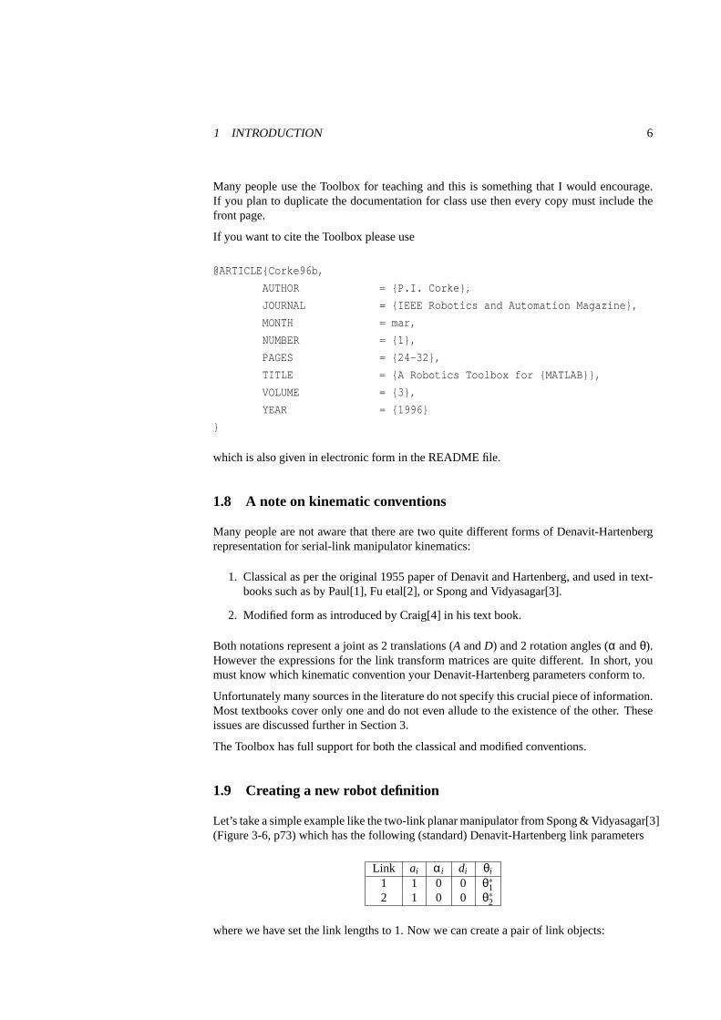
Let’s take a simple example like the two-link planar manipulator from Spong & Vidyasagar[3](Figure 3-6, p73) which has the following (standard) Denavit-Hartenberg link parameters
Link ai αi di θi
1 1 0 0 θ∗12 1 0 0 θ∗2
where we have set the link lengths to 1. Now we can create a pairof link objects:
1 INTRODUCTION 7
>> L1=link([0 1 0 0 0], ’standard’)
L1 =
0.000000 1.000000 0.000000 0.000000 R (std)
>> L2=link([0 1 0 0 0], ’standard’)
L2 =
0.000000 1.000000 0.000000 0.000000 R (std)
>> r=robot(L1 L2)
r =
noname (2 axis, RR)
grav = [0.00 0.00 9.81] standard D&H parameters
alpha A theta D R/P
0.000000 1.000000 0.000000 0.000000 R (std)
0.000000 1.000000 0.000000 0.000000 R (std)
>>
The first few lines create link objects, one per robot link. Note the second argument tolink which specifies that the standard D&H conventions are to be used (this is actually thedefault). The arguments to the link object can be found from
>> help link
.
.
LINK([alpha A theta D sigma], CONVENTION)
.
.
which shows the order in which the link parameters must be passed (which is different tothe column order of the table above). The fifth element of the first argument,sigma , is aflag that indicates whether the joint is revolute (sigma is zero) or primsmatic (sigma is nonzero).
The link objects are passed as a cell array to therobot() function which creates a robotobject which is in turn passed to many of the other Toolbox functions.
Note that displays of link data include the kinematic convention in brackets on the far right.(std) for standard form, and(mod) for modified form.
The robot just created can be displayed graphically by
1 INTRODUCTION 8
−2
−1
0
1
2
−2
−1
0
1
2−2
−1.5
−1
−0.5
0
0.5
1
1.5
2
XY
Z
noname
xy z
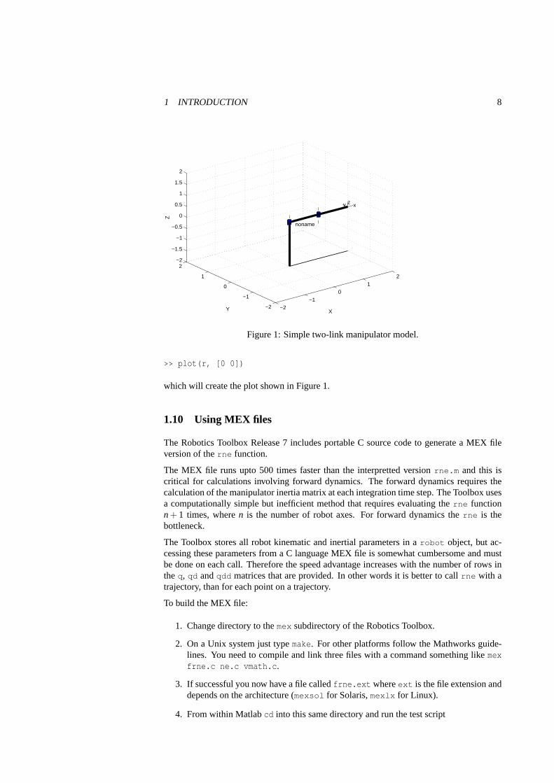
Figure 1: Simple two-link manipulator model.
>> plot(r, [0 0])
which will create the plot shown in Figure 1.
1.10 Using MEX files
The Robotics Toolbox Release 7 includes portable C source code to generate a MEX fileversion of therne function.
The MEX file runs upto 500 times faster than the interpretted versionrne.m and this iscritical for calculations involving forward dynamics. Theforward dynamics requires thecalculation of the manipulator inertia matrix at each integration time step. The Toolbox usesa computationally simple but inefficient method that requires evaluating therne functionn + 1 times, wheren is the number of robot axes. For forward dynamics therne is thebottleneck.
The Toolbox stores all robot kinematic and inertial parameters in arobot object, but ac-cessing these parameters from a C language MEX file is somewhat cumbersome and mustbe done on each call. Therefore the speed advantage increases with the number of rows intheq, qd andqdd matrices that are provided. In other words it is better to call rne with atrajectory, than for each point on a trajectory.
To build the MEX file:
1. Change directory to themex subdirectory of the Robotics Toolbox.
2. On a Unix system just typemake. For other platforms follow the Mathworks guide-lines. You need to compile and link three files with a command something likemexfrne.c ne.c vmath.c .
3. If successful you now have a file calledfrne.ext whereext is the file extension anddepends on the architecture (mexsol for Solaris,mexlx for Linux).
4. From within Matlabcd into this same directory and run the test script
1 INTRODUCTION 9
>> cd ROBOTDIR/mex
>> check
*************************************************** ************
************************ Puma 560 ******************** *********
*************************************************** ************
************************ normal case ***************** ************
DH: Fast RNE: (c) Peter Corke 2002
Speedup is 17, worst case error is 0.000000
MDH: Speedup is 1565, worst case error is 0.000000
************************ no gravity ****************** ***********
DH: Speedup is 1501, worst case error is 0.000000
MDH: Speedup is 1509, worst case error is 0.000000
************************ ext force ******************* **********
DH: Speedup is 1497, worst case error is 0.000000
MDH: Speedup is 637, worst case error is 0.000000
*************************************************** ************
********************** Stanford arm ****************** *********
*************************************************** ************
************************ normal case ***************** ************
DH: Speedup is 1490, worst case error is 0.000000
MDH: Speedup is 1519, worst case error is 0.000000
************************ no gravity ****************** ***********
DH: Speedup is 1471, worst case error is 0.000000
MDH: Speedup is 1450, worst case error is 0.000000
************************ ext force ******************* **********
DH: Speedup is 417, worst case error is 0.000000
MDH: Speedup is 1458, worst case error is 0.000000
>>
This will run the M-file and MEX-file versions of therne function for various robotmodels and options with various options. For each case it should report a speedupgreater than one, and an error of zero. The results shown above are for a Sparc Ultra10.
5. Copy the MEX-filefrne.ext into the Robotics Toolbox main directory with thenamerne.ext . Thus all future references torne will now invoke the MEX-fileinstead of the M-file. The first time you run the MEX-file in any Matlab session itwill print a one-line identification message.
10
2Using the Toolbox with Simulink
2 Introduction
Simulink is the block diagram editing and simulation environment for Matlab. Until itsmost recent release Simulink has not been able to handle matrix valued signals, and that hasmade its application to robotics somewhat clumsy. This shortcoming has been rectified withSimulink Release 4. Robot Toolbox Release 7 and higher includes a library of blocks foruse in constructing robot kinematic and dynamic models.
To use this new feature it is neccessary to include the Toolbox Simulink block directory inyour Matlab path:
>> addpath ROBOTDIR/simulink
To bring up the block library
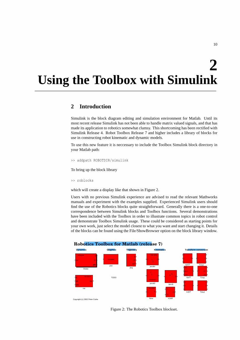
>> roblocks
which will create a display like that shown in Figure 2.
Users with no previous Simulink experience are advised to read the relevant Mathworksmanuals and experiment with the examples supplied. Experienced Simulink users shouldfind the use of the Robotics blocks quite straightforward. Generally there is a one-to-onecorrespondence between Simulink blocks and Toolbox functions. Several demonstrationshave been included with the Toolbox in order to illustrate common topics in robot controland demonstrate Toolbox Simulink usage. These could be considered as starting points foryour own work, just select the model closest to what you want and start changing it. Detailsof the blocks can be found using the File/ShowBrowser optionon the block library window.
Robotics Toolbox for Matlab (release 7)
TODO
Copyright (c) 2002 Peter Corke
Dynamics Graphics Kinematics Transform conversionTrajectory
x
y
z
T
xyz2T
T1
T2
dx
tr2diff
roll
pitch
yaw
T
rpy2T
tau
q
qd
qdd
noname
rne
noname
plot
q
qd
qdd
jtraj
Jn
noname
q J
jacobn
J0
noname
q J
jacob0
J−1
J Ji
ijacob
q T
noname
fkine
a
b
c
T
eul2T
T
x
y
z
T2xyz
T
roll
pitch
yaw
T2rpy
T
a
b
c
T2eul
tau
q
qd
qdd
noname
Robot
Figure 2: The Robotics Toolbox blockset.

3 EXAMPLES 11
Puma560 collapsing under gravity
Puma 560
plot[0 0 0 0 0 0]’
Zerotorque
simout
To Workspace
tau
q
qd
qdd
Puma 560
Robot
Simple dynamics demopic11−Feb−2002 14:19:49
0
Clock
Figure 3: Robotics Toolbox exampledemo1, Puma robot collapsing under gravity.
3 Examples
3.1 Dynamic simulation of Puma 560 robot collapsing under gravity
The Simulink model,demo1, is shown in Figure 3, and the two blocks in this model wouldbe familiar to Toolbox users. TheRobot block is similar to thefdyn() function and repre-sents the forward dynamics of the robot, and theplot block represents theplot function.Note the parameters of theRobot block contain the robot object to be simulated and theinitial joint angles. Theplot block has one parameter which is the robot object to be dis-played graphically and should be consistent with the robot being simulated. Display optionsare taken from theplotbotopt.m file, see help forrobot/plot for details.
To run this demo first create a robot object in the workspace,typically by using thepuma560
command, then start the simulation using Simulation/Startoption from the model toolbar.
>> puma560
>> demo1
3.2 Dynamic simulation of a simple robot with flexible transmission
The Simulink model,demo2, is shown in Figure 4, and represents a simple 2-link robot withflexible or compliant transmission. The first joint receivesa step position demand change attime 1s. The resulting oscillation and dynamic coupling between the two joints can be seenclearly. Note that the drive model comprises spring plus damper, and that the joint positioncontrol loops are simply unity negative feedback.
To run this demo first create a 2-link robot object in the workspace,typically by using thetwolink command, then start the simulation using Simulation/Startoption from the modeltoolbar.
>> twolink
>> demo2
3 EXAMPLES 12
2−link robot with flexible transmission
load position
transmission comprisesspring + damper
assume the motoris infinitely "stiff"
Puma 560
plot
simout
To Workspace
Step
Scope
tau
q
qd
qdd
Puma 560
Robot
Rate Limiter
2−link demopicMon Apr 8 11:37:04 2002
100
K
du/dt
Derivative
0
Constant
0
Clock
20
B
motorposition
Figure 4: Robotics Toolbox exampledemo2, simple flexible 2-link manipulator.
3.3 Computed torque control
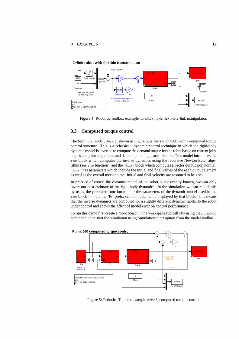
The Simulink model,demo3, shown in Figure 5, is for a Puma560 with a computed torquecontrol structure. This is a “classical” dynamic control technique in which the rigid-bodydynamic model is inverted to compute the demand torque for the robot based on current jointangles and joint angle rates and demand joint angle acceleration. This model introduces therne block which computes the inverse dynamics using the recursive Newton-Euler algo-rithm (seerne function), and thejtraj block which computes a vector quintic polynomial.jtraj has parameters which include the initial and final values of the each output elementas well as the overall motion time. Initial and final velocityare assumed to be zero.
In practice of course the dynamic model of the robot is not exactly known, we can onlyinvert our best estimate of the rigid-body dynamics. In the simulation we can model thisby using theperturb function to alter the parameters of the dynamic model used intherne block — note the ’P/’ prefix on the model name displayed by thatblock. This meansthat the inverse dynamics are computed for a slightly different dynamic model to the robotunder control and shows the effect of model error on control performance.
To run this demo first create a robot object in the workspace,typically by using thepuma560
command, then start the simulation using Simulation/Startoption from the model toolbar.
Puma 560 computed torque control
trajectory(demand)
robot state(actual)
error
tau
q
qd
qdd
P/Puma 560
rne
Puma 560
plot
q
qd
qdd
jtraj
simout
To Workspace
tau
q
qd
qdd
Puma 560
Robot
Puma560 computed torque controlpic11−Feb−2002 14:18:39
100
Kp
1
Kd
0
Clock
Figure 5: Robotics Toolbox exampledemo3, computed torque control.
3 EXAMPLES 13
>> puma560
>> demo3
3.4 Torque feedforward control
The Simulink modeldemo4 demonstrates torque feedforward control, another “classical”dynamic control technique in which the demanded torque is computed using therne blockand added to the error torque computed from position and velocity error. It is instructive tocompare the structure of this model withdemo3. The inverse dynamics are not in the for-ward path and since the robot configuration changes relatively slowly, they can be computedat a low rate (this is illustrated by the zero-order hold block sampling at 20Hz).
To run this demo first create a robot object in the workspace,typically by using thepuma560
command, then start the simulation using Simulation/Startoption from the model toolbar.
>> puma560
>> demo4
3.5 Cartesian space control
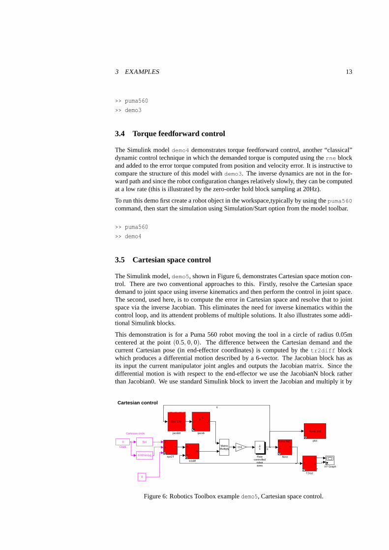
The Simulink model,demo5, shown in Figure 6, demonstrates Cartesian space motion con-trol. There are two conventional approaches to this. Firstly, resolve the Cartesian spacedemand to joint space using inverse kinematics and then perform the control in joint space.The second, used here, is to compute the error in Cartesian space and resolve that to jointspace via the inverse Jacobian. This eliminates the need forinverse kinematics within thecontrol loop, and its attendent problems of multiple solutions. It also illustrates some addi-tional Simulink blocks.
This demonstration is for a Puma 560 robot moving the tool in acircle of radius 0.05mcentered at the point(0.5, 0, 0). The difference between the Cartesian demand and thecurrent Cartesian pose (in end-effector coordinates) is computed by thetr2diff blockwhich produces a differential motion described by a 6-vector. The Jacobian block has asits input the current manipulator joint angles and outputs the Jacobian matrix. Since thedifferential motion is with respect to the end-effector we use the JacobianN block ratherthan Jacobian0. We use standard Simulink block to invert theJacobian and multiply it by
Cartesian circle
Cartesian control
x
y
z
T
xyz2T
T1
T2
dx
tr2diff
Puma 560
plot
Bad Link
jacob0
J−1
J Ji
ijacob
q T
Puma 560
fkine
XY GraphT
x
y
z
T2xyz
1s
Ratecontrolled
robotaxes
MatrixMultiply
−0.6
0.05*sin(u)
f(u)
0
0
Clock
q
q
Figure 6: Robotics Toolbox exampledemo5, Cartesian space control.
3 EXAMPLES 14
the differential motion. The result, after application of asimple proportional gain, is thejoint space motion required to correct the Cartesian error.The robot is modelled by anintegrator as a simple rate control device, or velocity servo.
This example also demonstrates the use of thefkine block for forward kinematics and theT2xyz block which extracts the translational part of the robot’s Cartesian state for plottingon the XY plane.
This demonstration is very similar to the numerical method used to solve the inverse kine-matics problem inikine .
To run this demo first create a robot object in the workspace,typically by using thepuma560
command, then start the simulation using Simulation/Startoption from the model toolbar.
>> puma560
>> demo5
3.6 Image-based visual servoing
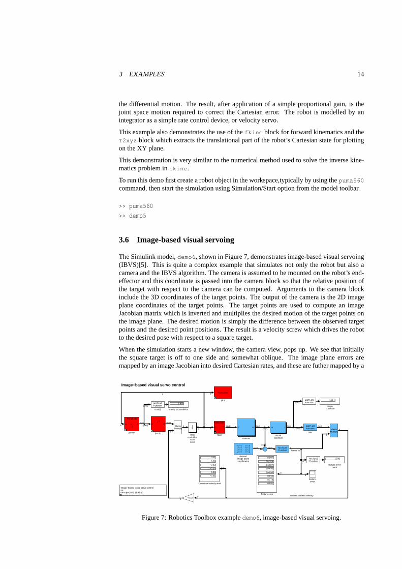
The Simulink model,demo6, shown in Figure 7, demonstrates image-based visual servoing(IBVS)[5]. This is quite a complex example that simulates not only the robot but also acamera and the IBVS algorithm. The camera is assumed to be mounted on the robot’s end-effector and this coordinate is passed into the camera blockso that the relative position ofthe target with respect to the camera can be computed. Arguments to the camera blockinclude the 3D coordinates of the target points. The output of the camera is the 2D imageplane coordinates of the target points. The target points are used to compute an imageJacobian matrix which is inverted and multiplies the desired motion of the target points onthe image plane. The desired motion is simply the differencebetween the observed targetpoints and the desired point positions. The result is a velocity screw which drives the robotto the desired pose with respect to a square target.
When the simulation starts a new window, the camera view, popsup. We see that initiallythe square target is off to one side and somewhat oblique. Theimage plane errors aremapped by an image Jacobian into desired Cartesian rates, and these are futher mapped by a
Image−based visual servo control
desired camera velocity
uv J
visualJacobian
146.1
visjaccondition
Puma 560
plot
MATLABFunction
pinv
6.998
manip jac condition
Jn
Puma 560
q J
jacobn
J−1
J Ji
ijacob
q T
Puma 560
fkine
274
feature errornorm
85.07
107.89
112.87
109.40
108.90
80.92
81.10
80.81
feature error
feature error
256 456456 456456 256256 256
desiredimage planecoordinates
MATLABFunction
cond()
T uv
camera
1s
Ratecontrolled
robotaxes
MatrixMultiply
MatrixMultiply
Image−based visual servo controlpic08−Apr−2002 11:31:20
MATLABFunction
MATLABFunction
MATLABFunction
−0.10
0.21
0.28
−0.32
−0.00
0.04
−0.01
Cartesian velocity dmd
6
q 6
66q
[6x6]
[6x6]
[6x6]
6
[4x2]
[4x2][4x2][4x4]
[8x6]
[8x6][8x6]
[4x2]
[6x8]
[4x2]
88
8
8
8feature vel
[6x6]
6
6
6
6
6
Figure 7: Robotics Toolbox exampledemo6, image-based visual servoing.

3 EXAMPLES 15
manipulator Jacobian into joint rates which are applied to the robot which is again modelledas a rate control device. This closed-loop system is performing a Cartesian positioning taskusing information from a camera rather than encoders and a kinematic model (the Jacobianis a weak kinematic model). Image-based visual servoing schemes have been found to beextremely robust with respect to errors in the camera model and manipulator Jacobian.
16
3Tutorial
3 Manipulator kinematics
Kinematics is the study of motion without regard to the forces which cause it. Within kine-matics one studies the position, velocity and acceleration, and all higher order derivatives ofthe position variables. The kinematics of manipulators involves the study of the geometricand time based properties of the motion, and in particular how the various links move withrespect to one another and with time.
Typical robots areserial-link manipulators comprising a set of bodies, calledlinks, in achain, connected byjoints1. Each joint has one degree of freedom, either translationalorrotational. For a manipulator withn joints numbered from 1 ton, there aren + 1 links,numbered from 0 ton. Link 0 is the base of the manipulator, generally fixed, and link ncarries the end-effector. Jointi connects linksi andi−1.
A link may be considered as a rigid body defining the relationship between two neighbour-ing joint axes. A link can be specified by two numbers, thelink length andlink twist, whichdefine the relative location of the two axes in space. The linkparameters for the first andlast links are meaningless, but are arbitrarily chosen to be0. Joints may be described bytwo parameters. Thelink offset is the distance from one link to the next along the axis of thejoint. Thejoint angle is the rotation of one link with respect to the next about the joint axis.
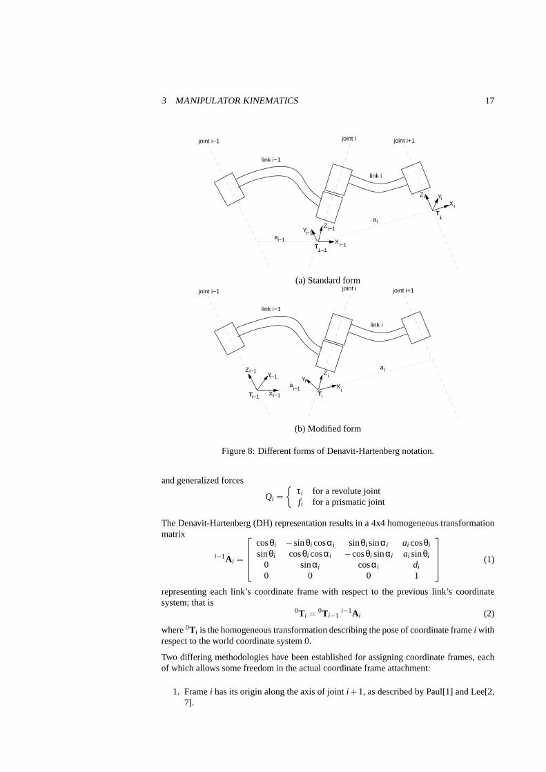
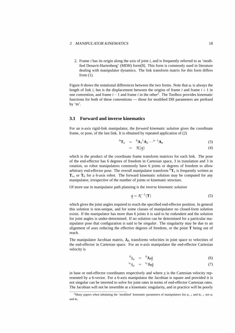
To facilitate describing the location of each link we affix a coordinate frame to it — frameiis attached to linki. Denavit and Hartenberg[6] proposed a matrix method of systematicallyassigning coordinate systems to each link of an articulatedchain. The axis of revolute jointi is aligned withzi−1. The xi−1 axis is directed along the normal fromzi−1 to zi and forintersecting axes is parallel tozi−1× zi. The link and joint parameters may be summarizedas:
link length ai the offset distance between thezi−1 andzi axes along thexi axis;
link twist αi the angle from thezi−1 axis to thezi axis about thexi axis;link offset di the distance from the origin of framei−1 to thexi axis
along thezi−1 axis;joint angle θi the angle between thexi−1 andxi axes about thezi−1 axis.
For a revolute axisθi is the joint variable anddi is constant, while for a prismatic jointdi
is variable, andθi is constant. In many of the formulations that follow we use generalizedcoordinates,qi, where
qi =
θi for a revolute jointdi for a prismatic joint
1Parallel link and serial/parallel hybrid structures are possible, though much less common in industrial manip-
ulators.
3 MANIPULATOR KINEMATICS 17
joint i−1 joint i joint i+1
link i−1
link i
Ti−1
Tiai
X i
YiZ i
ai−1
Z i−1
X i−1
Yi−1
(a) Standard formjoint i−1 joint i joint i+1
link i−1
link i
Ti−1 TiX i−1
Yi−1Zi−1
YiX
i
Z i
ai−1
a i
(b) Modified form
Figure 8: Different forms of Denavit-Hartenberg notation.
and generalized forces
Qi =
τi for a revolute jointfi for a prismatic joint
The Denavit-Hartenberg (DH) representation results in a 4x4 homogeneous transformationmatrix
i−1Ai =
cosθi −sinθi cosαi sinθi sinαi ai cosθi
sinθi cosθi cosαi −cosθi sinαi ai sinθi
0 sinαi cosαi di
0 0 0 1
(1)
representing each link’s coordinate frame with respect to the previous link’s coordinatesystem; that is
0Ti = 0Ti−1i−1Ai (2)
where0Ti is the homogeneous transformation describing the pose of coordinate framei withrespect to the world coordinate system 0.
Two differing methodologies have been established for assigning coordinate frames, eachof which allows some freedom in the actual coordinate frame attachment:
1. Framei has its origin along the axis of jointi+1, as described by Paul[1] and Lee[2,7].
3 MANIPULATOR KINEMATICS 18
2. Framei has its origin along the axis of jointi, and is frequently referred to as ‘modi-fied Denavit-Hartenberg’ (MDH) form[8]. This form is commonly used in literaturedealing with manipulator dynamics. The link transform matrix for this form differsfrom (1).
Figure 8 shows the notational differences between the two forms. Note thatai is always thelength of link i, but is the displacement between the origins of framei and framei + 1 inone convention, and framei−1 and framei in the other2. The Toolbox provides kinematicfunctions for both of these conventions — those for modified DH parameters are prefixedby ‘m’.
3.1 Forward and inverse kinematics
For an n-axis rigid-link manipulator, theforward kinematic solution gives the coordinateframe, or pose, of the last link. It is obtained by repeated application of (2)
0Tn = 0A11A2 · · ·
n−1An (3)
= K (q) (4)
which is the product of the coordinate frame transform matrices for each link. The poseof the end-effector has 6 degrees of freedom in Cartesian space, 3 in translation and 3 inrotation, so robot manipulators commonly have 6 joints or degrees of freedom to allowarbitrary end-effector pose. The overall manipulator transform0Tn is frequently written asTn, or T6 for a 6-axis robot. The forward kinematic solution may be computed for anymanipulator, irrespective of the number of joints or kinematic structure.
Of more use in manipulator path planning is theinverse kinematic solution
q =K −1(T) (5)
which gives the joint angles required to reach the specified end-effector position. In generalthis solution is non-unique, and for some classes of manipulator no closed-form solutionexists. If the manipulator has more than 6 joints it is said toberedundant and the solutionfor joint angles is under-determined. If no solution can be determined for a particular ma-nipulator pose that configuration is said to besingular. The singularity may be due to analignment of axes reducing the effective degrees of freedom, or the pointT being out ofreach.
The manipulator Jacobian matrix,Jθ, transforms velocities in joint space to velocities ofthe end-effector in Cartesian space. For ann-axis manipulator the end-effector Cartesianvelocity is
0xn = 0Jθq (6)tn xn = tnJθq (7)
in base or end-effector coordinates respectively and wherex is the Cartesian velocity rep-resented by a 6-vector. For a 6-axis manipulator the Jacobian is square and provided it isnot singular can be inverted to solve for joint rates in termsof end-effector Cartesian rates.The Jacobian will not be invertible at a kinematic singularity, and in practice will be poorly
2Many papers when tabulating the ‘modified’ kinematic parameters of manipulators listai−1 andαi−1 not ai
andαi.
4 MANIPULATOR RIGID-BODY DYNAMICS 19
conditioned in the vicinity of the singularity, resulting in high joint rates. A control schemebased on Cartesian rate control
q = 0J−1θ
0xn (8)
was proposed by Whitney[9] and is known asresolved rate motion control. For two framesA andB related byATB = [n o a p] the Cartesian velocity in frameA may be transformed toframeB by
Bx = BJAAx (9)
where the Jacobian is given by Paul[10] as
BJA = f (ATB) =
[
[n o a]T [p×n p×o p×a]T
0 [n o a]T
]
(10)
4 Manipulator rigid-body dynamics
Manipulator dynamics is concerned with the equations of motion, the way in which themanipulator moves in response to torques applied by the actuators, or external forces. Thehistory and mathematics of the dynamics of serial-link manipulators is well covered byPaul[1] and Hollerbach[11]. There are two problems relatedto manipulator dynamics thatare important to solve:
• inverse dynamics in which the manipulator’s equations of motion are solved for givenmotion to determine the generalized forces, discussed further in Section 4.1, and
• direct dynamics in which the equations of motion are integrated to determinethegeneralized coordinate response to applied generalized forces discussed further inSection 4.2.
The equations of motion for ann-axis manipulator are given by
Q = M(q)q+C(q, q)q+F(q)+G(q) (11)
where
q is the vector of generalized joint coordinates describing the pose of the manipulatorq is the vector of joint velocities;q is the vector of joint accelerations
M is the symmetric joint-space inertia matrix, or manipulator inertia tensorC describes Coriolis and centripetal effects — Centripetal torques are proportional to ˙q2
i ,while the Coriolis torques are proportional to ˙qiq j
F describes viscous and Coulomb friction and is not generallyconsidered part of the rigid-body dynamics
G is the gravity loadingQ is the vector of generalized forces associated with the generalized coordinatesq.
The equations may be derived via a number of techniques, including Lagrangian (energybased), Newton-Euler, d’Alembert[2, 12] or Kane’s[13] method. The earliest reported workwas by Uicker[14] and Kahn[15] using the Lagrangian approach. Due to the enormous com-putational cost,O(n4), of this approach it was not possible to compute manipulatortorquefor real-time control. To achieve real-time performance many approaches were suggested,including table lookup[16] and approximation[17, 18]. Themost common approximationwas to ignore the velocity-dependent termC, since accurate positioning and high speedmotion are exclusive in typical robot applications.
4 MANIPULATOR RIGID-BODY DYNAMICS 20
Method Multiplications Additions For N=6
Multiply Add
Lagrangian[22] 3212n4 +86 5
12n3 25n4 +6613n3 66,271 51,548
+17114n2 +531
3n +12912n2 +421
3n
−128 −96
Recursive NE[22] 150n−48 131n−48 852 738
Kane[13] 646 394
Simplified RNE[25] 224 174
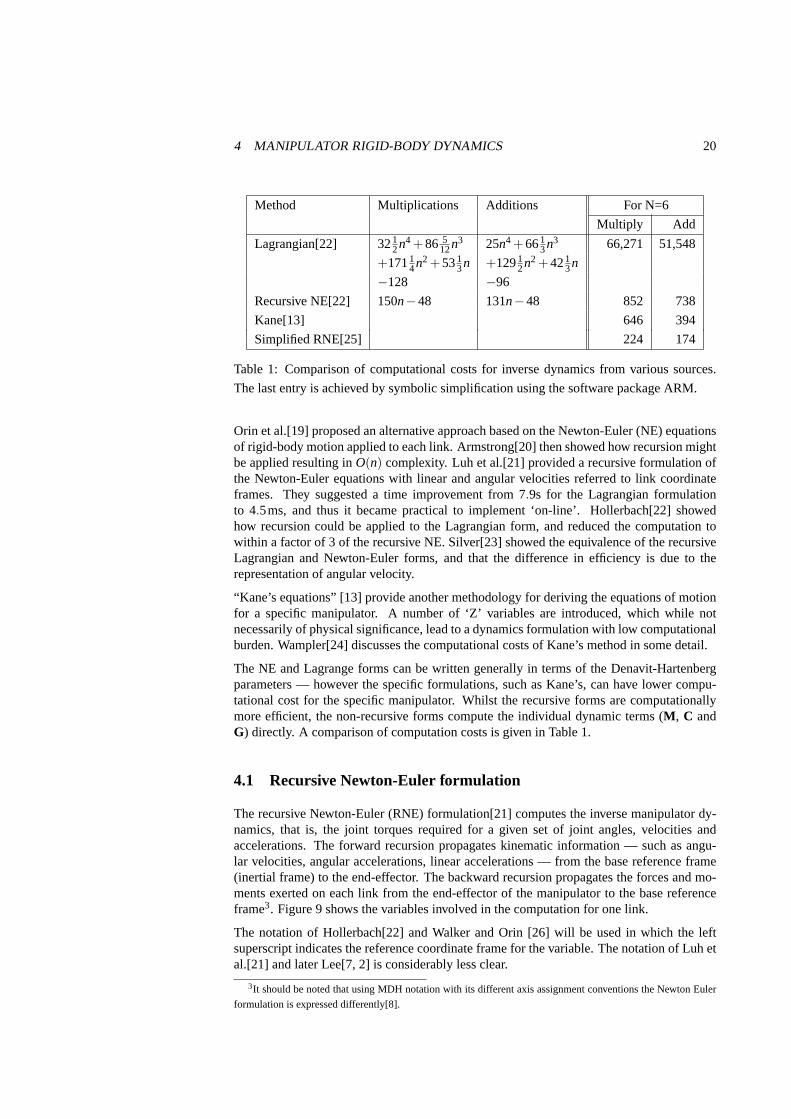
Table 1: Comparison of computational costs for inverse dynamics from various sources.
The last entry is achieved by symbolic simplification using the software package ARM.
Orin et al.[19] proposed an alternative approach based on the Newton-Euler (NE) equationsof rigid-body motion applied to each link. Armstrong[20] then showed how recursion mightbe applied resulting inO(n) complexity. Luh et al.[21] provided a recursive formulation ofthe Newton-Euler equations with linear and angular velocities referred to link coordinateframes. They suggested a time improvement from 7.9s for the Lagrangian formulationto 4.5ms, and thus it became practical to implement ‘on-line’. Hollerbach[22] showedhow recursion could be applied to the Lagrangian form, and reduced the computation towithin a factor of 3 of the recursive NE. Silver[23] showed the equivalence of the recursiveLagrangian and Newton-Euler forms, and that the differencein efficiency is due to therepresentation of angular velocity.
“Kane’s equations” [13] provide another methodology for deriving the equations of motionfor a specific manipulator. A number of ‘Z’ variables are introduced, which while notnecessarily of physical significance, lead to a dynamics formulation with low computationalburden. Wampler[24] discusses the computational costs of Kane’s method in some detail.
The NE and Lagrange forms can be written generally in terms ofthe Denavit-Hartenbergparameters — however the specific formulations, such as Kane’s, can have lower compu-tational cost for the specific manipulator. Whilst the recursive forms are computationallymore efficient, the non-recursive forms compute the individual dynamic terms (M , C andG) directly. A comparison of computation costs is given in Table 1.
4.1 Recursive Newton-Euler formulation
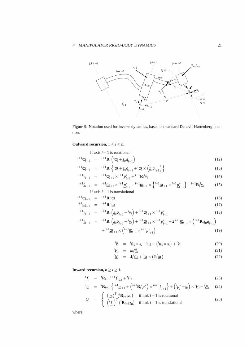
The recursive Newton-Euler (RNE) formulation[21] computes the inverse manipulator dy-namics, that is, the joint torques required for a given set ofjoint angles, velocities andaccelerations. The forward recursion propagates kinematic information — such as angu-lar velocities, angular accelerations, linear accelerations — from the base reference frame(inertial frame) to the end-effector. The backward recursion propagates the forces and mo-ments exerted on each link from the end-effector of the manipulator to the base referenceframe3. Figure 9 shows the variables involved in the computation for one link.
The notation of Hollerbach[22] and Walker and Orin [26] willbe used in which the leftsuperscript indicates the reference coordinate frame for the variable. The notation of Luh etal.[21] and later Lee[7, 2] is considerably less clear.
3It should be noted that using MDH notation with its differentaxis assignment conventions the Newton Euler
formulation is expressed differently[8].
4 MANIPULATOR RIGID-BODY DYNAMICS 21
joint i−1 joint i joint i+1
link i−1
link i
Ti−1
Tiai
X i
YiZ i
ai−1
Z i−1
X i−1
Yi−1p* vi
.vi
.ωiωi
n fi i
N Fi i
vi
.vi
_ _i+1 i+1
n f
si
Figure 9: Notation used for inverse dynamics, based on standard Denavit-Hartenberg nota-
tion.
Outward recursion, 1≤ i ≤ n.
If axis i+1 is rotationali+1ωi+1 = i+1Ri
(
iωi + z0qi+1
)
(12)
i+1ωi+1 = i+1Ri
iωi + z0qi+1
+ iωi ×(
z0qi+1
)
(13)
i+1vi+1 = i+1ωi+1×i+1p∗
i+1+ i+1Ri
ivi (14)
i+1vi+1 = i+1ωi+1×i+1p∗
i+1+ i+1ωi+1×
i+1ωi+1×i+1p∗
i+1
+ i+1Riivi (15)
If axis i+1 is translationali+1ωi+1 = i+1Ri
iωi (16)i+1ωi+1 = i+1Ri
iωi (17)
i+1vi+1 = i+1Ri
(
z0qi+1
+ ivi
)
+ i+1ωi+1×i+1p∗
i+1(18)
i+1vi+1 = i+1Ri
(
z0qi+1
+ ivi
)
+ i+1ωi+1×i+1p∗
i+1+2 i+1ωi+1×
(
i+1Riz0qi+1
)
+i+1ωi+1×(
i+1ωi+1×i+1p∗
i+1
)
(19)
ivi = iωi × si +iωi ×
iωi × si
+ ivi (20)iF i = mi
ivi (21)iNi = Ji
iωi +iωi ×
(
Jiiωi
)
(22)
Inward recursion, n ≥ i ≥ 1.
i fi
= iRi+1i+1 f
i+1+ iF i (23)
ini = iRi+1
i+1ni+1 +(
i+1Rii p∗
i
)
× ii+1 fi+1
+(
i p∗i+ si
)
× iF i +iNi (24)
Qi
=
(
ini
)T (
iRi+1z0
)
if link i+1 is rotational(
i fi
)T(
iRi+1z0
)
if link i+1 is translational(25)
where

4 MANIPULATOR RIGID-BODY DYNAMICS 22
i is the link index, in the range 1 tonJi is the moment of inertia of linki about its COMsi is the position vector of the COM of linki with respect to framei
ωi is the angular velocity of linkiωi is the angular acceleration of linkivi is the linear velocity of frameivi is the linear acceleration of frameivi is the linear velocity of the COM of linkivi is the linear acceleration of the COM of linkini is the moment exerted on linki by link i−1f
iis the force exerted on linki by link i−1
Ni is the total moment at the COM of linkiF i is the total force at the COM of linkiQ
iis the force or torque exerted by the actuator at jointi
i−1Ri is the orthonormal rotation matrix defining framei orientation with respect to framei−1. It is the upper 3×3 portion of the link transform matrix given in (1).
i−1Ri =
cosθi −cosαi sinθi sinαi sinθi
sinθi cosαi cosθi −sinαi cosθi
0 sinαi cosαi
(26)
iRi−1 = (i−1Ri)−1 = (i−1Ri)
T (27)
i p∗i
is the displacement from the origin of framei−1 to framei with respect to framei.
i p∗i=
ai
di sinαi
di cosαi
(28)
It is the negative translational part of(i−1Ai)−1.
z0 is a unit vector in Z direction,z0 = [0 0 1]
Note that the COM linear velocity given by equation (14) or (18) does not need to be com-puted since no other expression depends upon it. Boundary conditions are used to introducethe effect of gravity by setting the acceleration of the baselink
v0 = −g (29)
whereg is the gravity vector in the reference coordinate frame, generally acting in thenegative Z direction, downward. Base velocity is generallyzero
v0 = 0 (30)
ω0 = 0 (31)
ω0 = 0 (32)
At this stage the Toolbox only provides an implementation ofthis algorithm using the stan-dard Denavit-Hartenberg conventions.
4.2 Direct dynamics
Equation (11) may be used to compute the so-called inverse dynamics, that is, actuatortorque as a function of manipulator state and is useful for on-line control. For simulation
REFERENCES 23
the direct, integral orforward dynamic formulation is required giving joint motion in termsof input torques.
Walker and Orin[26] describe several methods for computingthe forward dynamics, andall make use of an existing inverse dynamics solution. Usingthe RNE algorithm for in-verse dynamics, the computational complexity of the forward dynamics using ‘Method 1’is O(n3) for an n-axis manipulator. Their other methods are increasingly more sophisticatedbut reduce the computational cost, though stillO(n3). Featherstone[27] has described the“articulated-body method” forO(n) computation of forward dynamics, however forn < 9it is more expensive than the approach of Walker and Orin. Another O(n) approach forforward dynamics has been described by Lathrop[28].
4.3 Rigid-body inertial parameters
Accurate model-based dynamic control of a manipulator requires knowledge of the rigid-body inertial parameters. Each link has ten independent inertial parameters:
• link mass,mi;
• three first moments, which may be expressed as the COM location, si, with respect tosome datum on the link or as a momentSi = misi;
• six second moments, which represent the inertia of the link about a given axis, typi-cally through the COM. The second moments may be expressed inmatrix or tensorform as
J =
Jxx Jxy Jxz
Jxy Jyy Jyz
Jxz Jyz Jzz
(33)
where the diagonal elements are themoments of inertia, and the off-diagonals areproducts of inertia. Only six of these nine elements are unique: three moments andthree products of inertia.
For any point in a rigid-body there is one set of axes known as theprincipal axes ofinertia for which the off-diagonal terms, or products, are zero. These axes are givenby the eigenvectors of the inertia matrix (33) and the eigenvalues are the principalmoments of inertia. Frequently the products of inertia of the robot links are zero dueto symmetry.
A 6-axis manipulator rigid-body dynamic model thus entails60 inertial parameters. Theremay be additional parameters per joint due to friction and motor armature inertia. Clearly,establishing numeric values for this number of parameters is a difficult task. Many parame-ters cannot be measured without dismantling the robot and performing careful experiments,though this approach was used by Armstrong et al.[29]. Most parameters could be derivedfrom CAD models of the robots, but this information is often considered proprietary andnot made available to researchers.
References
[1] R. P. Paul,Robot Manipulators: Mathematics, Programming, and Control. Cam-bridge, Massachusetts: MIT Press, 1981.
REFERENCES 24
[2] K. S. Fu, R. C. Gonzalez, and C. S. G. Lee,Robotics. Control, Sensing, Vision andIntelligence. McGraw-Hill, 1987.
[3] M. Spong and M. Vidyasagar,Robot Dynamics and Control. John Wiley and Sons,1989.
[4] J. J. Craig,Introduction to Robotics. Addison Wesley, 1986.
[5] S. Hutchinson, G. Hager, and P. Corke, “A tutorial on visual servo control,”IEEETransactions on Robotics and Automation, vol. 12, pp. 651–670, Oct. 1996.
[6] R. S. Hartenberg and J. Denavit, “A kinematic notation for lower pair mechanismsbased on matrices,”Journal of Applied Mechanics, vol. 77, pp. 215–221, June 1955.
[7] C. S. G. Lee, “Robot arm kinematics, dynamics and control,” IEEE Computer, vol. 15,pp. 62–80, Dec. 1982.
[8] J. J. Craig,Introduction to Robotics. Addison Wesley, second ed., 1989.
[9] D. Whitney, “The mathematics of coordinated control of prosthetic arms and manipu-lators,”ASME Journal of Dynamic Systems, Measurement and Control, vol. 20, no. 4,pp. 303–309, 1972.
[10] R. P. Paul, B. Shimano, and G. E. Mayer, “Kinematic control equations for simplemanipulators,”IEEE Trans. Syst. Man Cybern., vol. 11, pp. 449–455, June 1981.
[11] J. M. Hollerbach, “Dynamics,” inRobot Motion - Planning and Control (M. Brady,J. M. Hollerbach, T. L. Johnson, T. Lozano-Perez, and M. T. Mason, eds.), pp. 51–71,MIT, 1982.
[12] C. S. G. Lee, B. Lee, and R. Nigham, “Development of the generalized D’Alembertequations of motion for mechanical manipulators,” inProc. 22nd CDC, (San Antonio,Texas), pp. 1205–1210, 1983.
[13] T. Kane and D. Levinson, “The use of Kane’s dynamical equations in robotics,”Int. J.Robot. Res., vol. 2, pp. 3–21, Fall 1983.
[14] J. Uicker,On the Dynamic Analysis of Spatial Linkages Using 4 by 4 Matrices. PhDthesis, Dept. Mechanical Engineering and Astronautical Sciences, NorthWestern Uni-versity, 1965.
[15] M. Kahn, “The near-minimum time control of open-loop articulated kinematic link-ages,” Tech. Rep. AIM-106, Stanford University, 1969.
[16] M. H. Raibert and B. K. P. Horn, “Manipulator control using the configuration spacemethod,”The Industrial Robot, pp. 69–73, June 1978.
[17] A. Bejczy, “Robot arm dynamics and control,” Tech. Rep.NASA-CR-136935, NASAJPL, Feb. 1974.
[18] R. Paul, “Modelling, trajectory calculation and servoing of a computer controlledarm,” Tech. Rep. AIM-177, Stanford University, Artificial Intelligence Laboratory,1972.
[19] D. Orin, R. McGhee, M. Vukobratovic, and G. Hartoch, “Kinematics and kineticanalysis of open-chain linkages utilizing Newton-Euler methods,”Mathematical Bio-sciences. An International Journal, vol. 43, pp. 107–130, Feb. 1979.
REFERENCES 25
[20] W. Armstrong, “Recursive solution to the equations of motion of an n-link manipula-tor,” in Proc. 5th World Congress on Theory of Machines and Mechanisms, (Montreal),pp. 1343–1346, July 1979.
[21] J. Y. S. Luh, M. W. Walker, and R. P. C. Paul, “On-line computational scheme for me-chanical manipulators,”ASME Journal of Dynamic Systems, Measurement and Con-trol, vol. 102, pp. 69–76, 1980.
[22] J. Hollerbach, “A recursive Lagrangian formulation ofmanipulator dynamics and acomparative study of dynamics formulation complexity,”IEEE Trans. Syst. Man Cy-bern., vol. SMC-10, pp. 730–736, Nov. 1980.
[23] W. M. Silver, “On the equivalance of Lagrangian and Newton-Euler dynamics formanipulators,”Int. J. Robot. Res., vol. 1, pp. 60–70, Summer 1982.
[24] C. Wampler,Computer Methods in Manipulator Kinematics, Dynamics, and Control:a Comparative Study. PhD thesis, Stanford University, 1985.
[25] J. J. Murray,Computational Robot Dynamics. PhD thesis, Carnegie-Mellon Univer-sity, 1984.
[26] M. W. Walker and D. E. Orin, “Efficient dynamic computer simulation of roboticmechanisms,”ASME Journal of Dynamic Systems, Measurement and Control,vol. 104, pp. 205–211, 1982.
[27] R. Featherstone,Robot Dynamics Algorithms. Kluwer Academic Publishers, 1987.
[28] R. Lathrop, “Constrained (closed-loop) robot simulation by local constraint propoga-tion.,” in Proc. IEEE Int. Conf. Robotics and Automation, pp. 689–694, 1986.
[29] B. Armstrong, O. Khatib, and J. Burdick, “The explicit dynamic model and inertialparameters of the Puma 560 arm,” inProc. IEEE Int. Conf. Robotics and Automation,vol. 1, (Washington, USA), pp. 510–18, 1986.

1
0.4pt0pt
Robotics Toolbox Release 8 Peter Corke, December 2008
2
2Reference
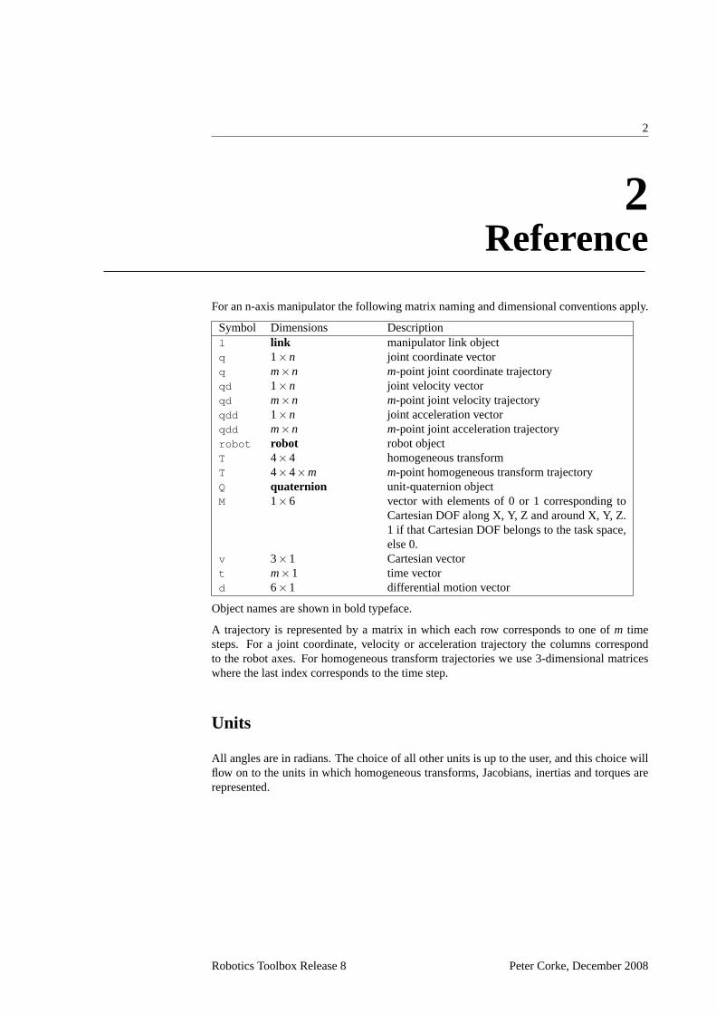
For an n-axis manipulator the following matrix naming and dimensional conventions apply.
Symbol Dimensions Descriptionl link manipulator link objectq 1×n joint coordinate vectorq m×n m-point joint coordinate trajectoryqd 1×n joint velocity vectorqd m×n m-point joint velocity trajectoryqdd 1×n joint acceleration vectorqdd m×n m-point joint acceleration trajectoryrobot robot robot objectT 4×4 homogeneous transformT 4×4×m m-point homogeneous transform trajectoryQ quaternion unit-quaternion objectM 1×6 vector with elements of 0 or 1 corresponding to
Cartesian DOF along X, Y, Z and around X, Y, Z.1 if that Cartesian DOF belongs to the task space,else 0.
v 3×1 Cartesian vectort m×1 time vectord 6×1 differential motion vector
Object names are shown in bold typeface.
A trajectory is represented by a matrix in which each row corresponds to one ofm timesteps. For a joint coordinate, velocity or acceleration trajectory the columns correspondto the robot axes. For homogeneous transform trajectories we use 3-dimensional matriceswhere the last index corresponds to the time step.
Units
All angles are in radians. The choice of all other units is up to the user, and this choice willflow on to the units in which homogeneous transforms, Jacobians, inertias and torques arerepresented.
Robotics Toolbox Release 8 Peter Corke, December 2008

Introduction 3
Homogeneous Transformsangvec2tr angle/vector form to homogeneous transformeul2tr Euler angle to homogeneous transformoa2tr orientation and approach vector to homogeneous transformrpy2tr Roll/pitch/yaw angles to homogeneous transformtr2angvec homogeneous transform or rotation matrix to angle/vector
formtr2eul homogeneous transform or rotation matrix to Euler anglest2r homogeneous transform to rotation submatrixtr2rpy homogeneous transform or rotation matrix to
roll/pitch/yaw anglestrotx homogeneous transform for rotation about X-axistroty homogeneous transform for rotation about Y-axistrotz homogeneous transform for rotation about Z-axistransl set or extract the translational component of a homoge-
neous transformtrnorm normalize a homogeneous transformtrplot plot a homogeneous transformas a coordinate frame
Note that functions of the formtr2X will also accept a rotation matrixas the argument.
Rotation matricesangvecr angle/vector form to rotation matrixeul2r Euler angle to rotation matrixoa2r orientation and approach vector to homogeneous transformrotx rotation matrix for rotation about X-axisroty rotation matrix for rotation about Y-axisrotz rotation matrix for rotation about Z-axisrpy2r Roll/pitch/yaw angles to rotation matrixr2t rotation matrix to homogeneous transform
Trajectory Generationctraj Cartesian trajectoryjtraj joint space trajectorytrinterp interpolate homogeneous transforms
Quaternions+ elementwise addition- elementwise addition/ divide quaternion by quaternion or scalar* multiply quaternion by a quaternion or vectorinv invert a quaternionnorm norm of a quaternionplot display a quaternion as a 3D rotationq2tr quaternion to homogeneous transformquaternion construct a quaternionqinterp interpolate quaternionsunit unitize a quaternion
Robotics Toolbox Release 8 Peter Corke, December 2008
Introduction 4
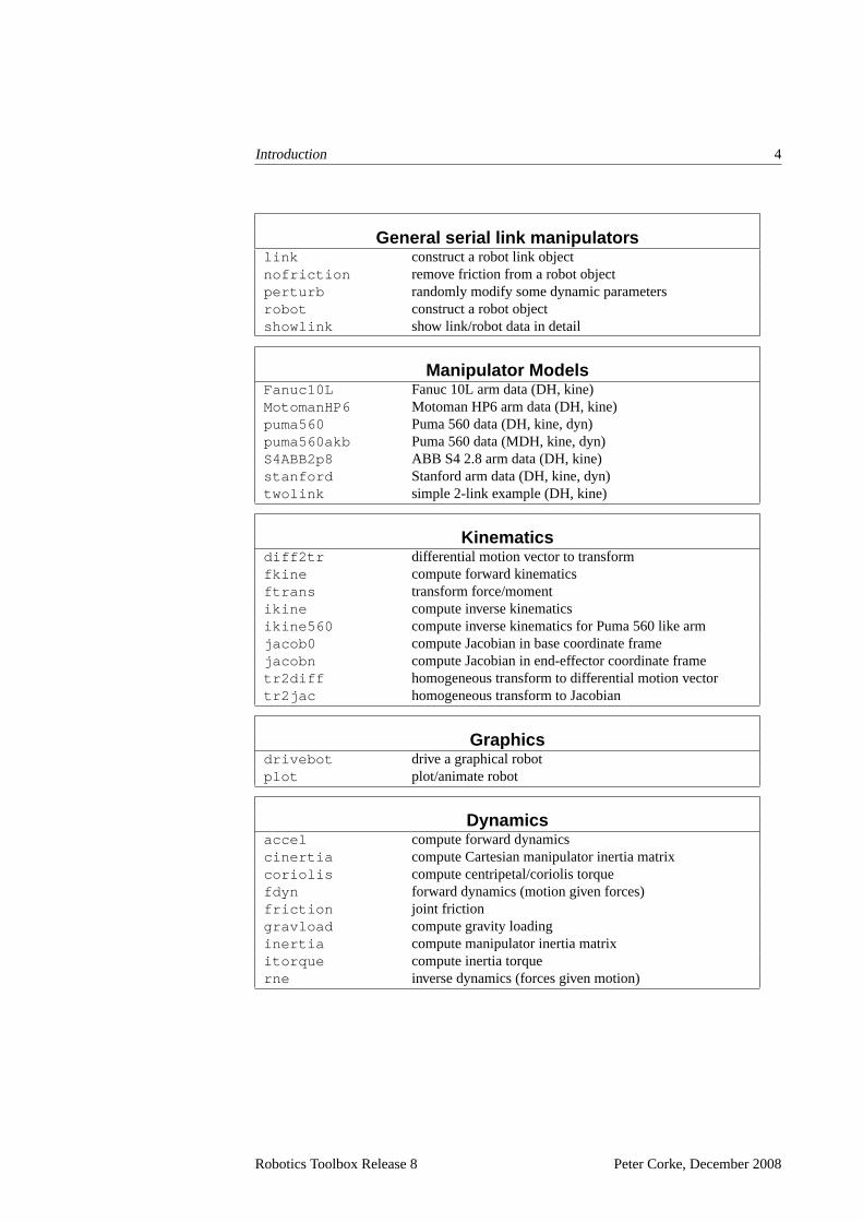
General serial link manipulatorslink construct a robot link objectnofriction remove friction from a robot objectperturb randomly modify some dynamic parametersrobot construct a robot objectshowlink show link/robot data in detail
Manipulator ModelsFanuc10L Fanuc 10L arm data (DH, kine)MotomanHP6 Motoman HP6 arm data (DH, kine)puma560 Puma 560 data (DH, kine, dyn)puma560akb Puma 560 data (MDH, kine, dyn)S4ABB2p8 ABB S4 2.8 arm data (DH, kine)stanford Stanford arm data (DH, kine, dyn)twolink simple 2-link example (DH, kine)
Kinematicsdiff2tr differential motion vector to transformfkine compute forward kinematicsftrans transform force/momentikine compute inverse kinematicsikine560 compute inverse kinematics for Puma 560 like armjacob0 compute Jacobian in base coordinate framejacobn compute Jacobian in end-effector coordinate frametr2diff homogeneous transform to differential motion vectortr2jac homogeneous transform to Jacobian
Graphicsdrivebot drive a graphical robotplot plot/animate robot
Dynamicsaccel compute forward dynamicscinertia compute Cartesian manipulator inertia matrixcoriolis compute centripetal/coriolis torquefdyn forward dynamics (motion given forces)friction joint frictiongravload compute gravity loadinginertia compute manipulator inertia matrixitorque compute inertia torquerne inverse dynamics (forces given motion)
Robotics Toolbox Release 8 Peter Corke, December 2008

Introduction 5
Otherishomog test if argument is 4×4isrot test if argument is 3×3isvec test if argument is a 3-vectormaniplty compute manipulabilityrtdemo toolbox demonstrationunit unitize a vector
Robotics Toolbox Release 8 Peter Corke, December 2008
accel 6
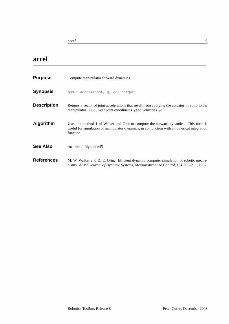
accel
Purpose Compute manipulator forward dynamics
Synopsis qdd = accel(robot, q, qd, torque)
Description Returns a vector of joint accelerations that result from applying the actuatortorque to themanipulatorrobot with joint coordinatesq and velocitiesqd.
Algorithm Uses the method 1 of Walker and Orin to compute the forward dynamics. This form isuseful for simulation of manipulator dynamics, in conjunction with a numerical integrationfunction.
See Also rne, robot, fdyn, ode45
References M. W. Walker and D. E. Orin. Efficient dynamic computer simulation of robotic mecha-nisms.ASME Journal of Dynamic Systems, Measurement and Control, 104:205–211, 1982.
Robotics Toolbox Release 8 Peter Corke, December 2008
angvec2tr, angvec2r 7
angvec2tr, angvec2r
Purpose Convert angle/vector form to a homogeneous transform or rotation matrix
Synopsis T = angvec2tr(theta, v)
R = angvec2r(theta, v)
Description Returns a homogeneous transform or rotation matrix representing a rotation oftheta radi-ans about the vectorv . For the homogeneous transform the translational component is setto zero.
See Also rotx, roty, rotz, quaternion
Robotics Toolbox Release 8 Peter Corke, December 2008
cinertia 8
cinertia
Purpose Compute the Cartesian (operational space) manipulator inertia matrix
Synopsis M = cinertia(robot, q)
Description cinertia computes the Cartesian, or operational space, inertia matrix. robot is a robotobject that describes the manipulator dynamics and kinematics, andq is an n-element vectorof joint coordinates.
Algorithm The Cartesian inertia matrix is calculated from the joint-space inertia matrix by
M(x) = J(q)−T M(q)J(q)−1
and relates Cartesian force/torque to Cartesian acceleration
F = M(x)x
See Also inertia, robot, rne
References O. Khatib, “A unified approach for motion and force control ofrobot manipulators: theoperational space formulation,”IEEE Trans. Robot. Autom., vol. 3, pp. 43–53, Feb. 1987.
Robotics Toolbox Release 8 Peter Corke, December 2008
coriolis 9
coriolis
Purpose Compute the manipulator Coriolis/centripetal torque components
Synopsis tau c = coriolis(robot, q, qd)
Description coriolis returns the joint torques due to rigid-body Coriolis and centripetal effects for thespecified joint stateq and velocityqd. robot is a robot object that describes the manipulatordynamics and kinematics.
If q andqd are row vectors,tau c is a row vector of joint torques. Ifq andqd are matrices,each row is interpreted as a joint state vector, andtau c is a matrix each row being thecorresponding joint torques.
Algorithm Evaluated from the equations of motion, usingrne , with joint acceleration and gravitationalacceleration set to zero,
τ = C(q, q)q
Joint friction is ignored in this calculation.
See Also robot, rne, itorque, gravload
References M. W. Walker and D. E. Orin. Efficient dynamic computer simulation of robotic mecha-nisms.ASME Journal of Dynamic Systems, Measurement and Control, 104:205–211, 1982.
Robotics Toolbox Release 8 Peter Corke, December 2008
ctraj 10
ctraj
Purpose Compute a Cartesian trajectory between two points
Synopsis TC = ctraj(T0, T1, m)
TC = ctraj(T0, T1, r)
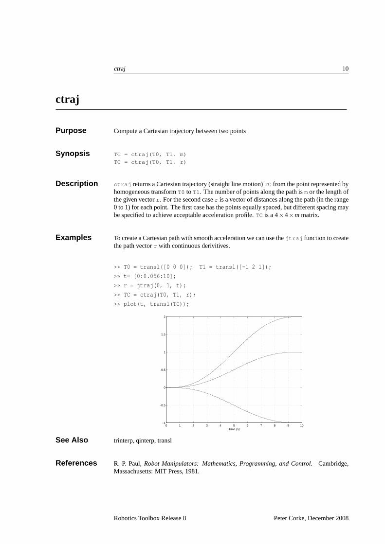
Description ctraj returns a Cartesian trajectory (straight line motion)TC from the point represented byhomogeneous transformT0 to T1. The number of points along the path ismor the length ofthe given vectorr . For the second caser is a vector of distances along the path (in the range0 to 1) for each point. The first case has the points equally spaced, but different spacing maybe specified to achieve acceptable acceleration profile.TC is a 4×4×m matrix.
Examples To create a Cartesian path with smooth acceleration we can use thejtraj function to createthe path vectorr with continuous derivitives.
>> T0 = transl([0 0 0]); T1 = transl([-1 2 1]);
>> t= [0:0.056:10];
>> r = jtraj(0, 1, t);
>> TC = ctraj(T0, T1, r);
>> plot(t, transl(TC));
0 1 2 3 4 5 6 7 8 9 10−1
−0.5
0
0.5
1
1.5
2
Time (s)
See Also trinterp, qinterp, transl
References R. P. Paul,Robot Manipulators: Mathematics, Programming, and Control. Cambridge,Massachusetts: MIT Press, 1981.
Robotics Toolbox Release 8 Peter Corke, December 2008
diff2tr 11
diff2tr
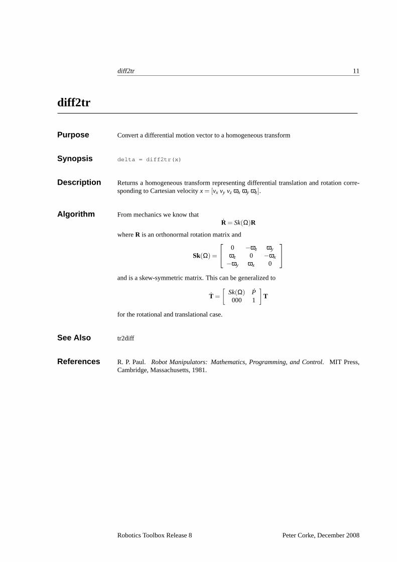
Purpose Convert a differential motion vector to a homogeneous transform
Synopsis delta = diff2tr(x)
Description Returns a homogeneous transform representing differential translation and rotation corre-sponding to Cartesian velocityx = [vx vy vz ωx ωy ωz].
Algorithm From mechanics we know thatR = Sk(Ω)R
whereR is an orthonormal rotation matrix and
Sk(Ω) =
0 −ωz ωy
ωz 0 −ωx
−ωy ωx 0
and is a skew-symmetric matrix. This can be generalized to
T =
[
Sk(Ω) P000 1
]
T
for the rotational and translational case.
See Also tr2diff
References R. P. Paul. Robot Manipulators: Mathematics, Programming, and Control. MIT Press,Cambridge, Massachusetts, 1981.
Robotics Toolbox Release 8 Peter Corke, December 2008

drivebot 12
drivebot
Purpose Drive a graphical robot
Synopsis drivebot(robot)
drivebot(robot, q)
Description Pops up a window with one slider for each joint. Operation of the sliders will drive thegraphical robot on the screen. Very useful for gaining an understanding of joint limits androbot workspace.
The joint coordinate state is kept with the graphical robot and can be obtained using theplot function. If q is specified it is used as the initial joint angle, otherwise the initial valueof joint coordinates is taken from the graphical robot.
Examples To drive a graphical Puma 560 robot
>> puma560 % define the robot
>> plot(p560,qz) % draw it
>> drivebot(p560) % now drive it
See Also robot/plot,robot
Robotics Toolbox Release 8 Peter Corke, December 2008
eul2tr, eul2r 13
eul2tr, eul2r
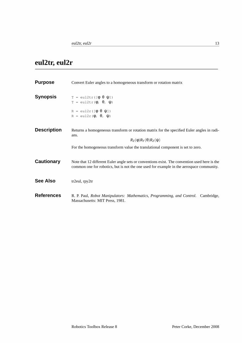
Purpose Convert Euler angles to a homogeneous transform or rotationmatrix
Synopsis T = eul2tr([ φ θ ψ])
T = eul2tr( φ, θ, ψ)
R = eul2r([ φ θ ψ])
R = eul2r( φ, θ, ψ)
Description Returns a homogeneous transform or rotation matrix for the specified Euler angles in radi-ans.
RZ(φ)RY (θ)RZ(ψ)
For the homogeneous transform value the translational component is set to zero.
Cautionary Note that 12 different Euler angle sets or conventions exist. The convention used here is thecommon one for robotics, but is not the one used for example inthe aerospace community.
See Also tr2eul, rpy2tr
References R. P. Paul,Robot Manipulators: Mathematics, Programming, and Control. Cambridge,Massachusetts: MIT Press, 1981.
Robotics Toolbox Release 8 Peter Corke, December 2008
Fanuc10L 14
Fanuc10L
Purpose Create a Fanuc 10L robot object
Synopsis Fanuc10L
Description Creates therobot objectRwhich describes the kinematic characteristics of a AM120iB/10Lmanipulator. The kinematic conventions used are as per Pauland Zhang, and all quantitiesare in standard SI units.
Also defined is the joint coordinate vectorq0 corresponding to the mastering position.
See Also robot, puma560akb, stanford, MotomanHP6, S4ABB2p8
Author Wynand Swart, Mega Robots CC, P/O Box 8412, Pretoria, 0001, South Africa,[email protected]
Robotics Toolbox Release 8 Peter Corke, December 2008
fdyn 15
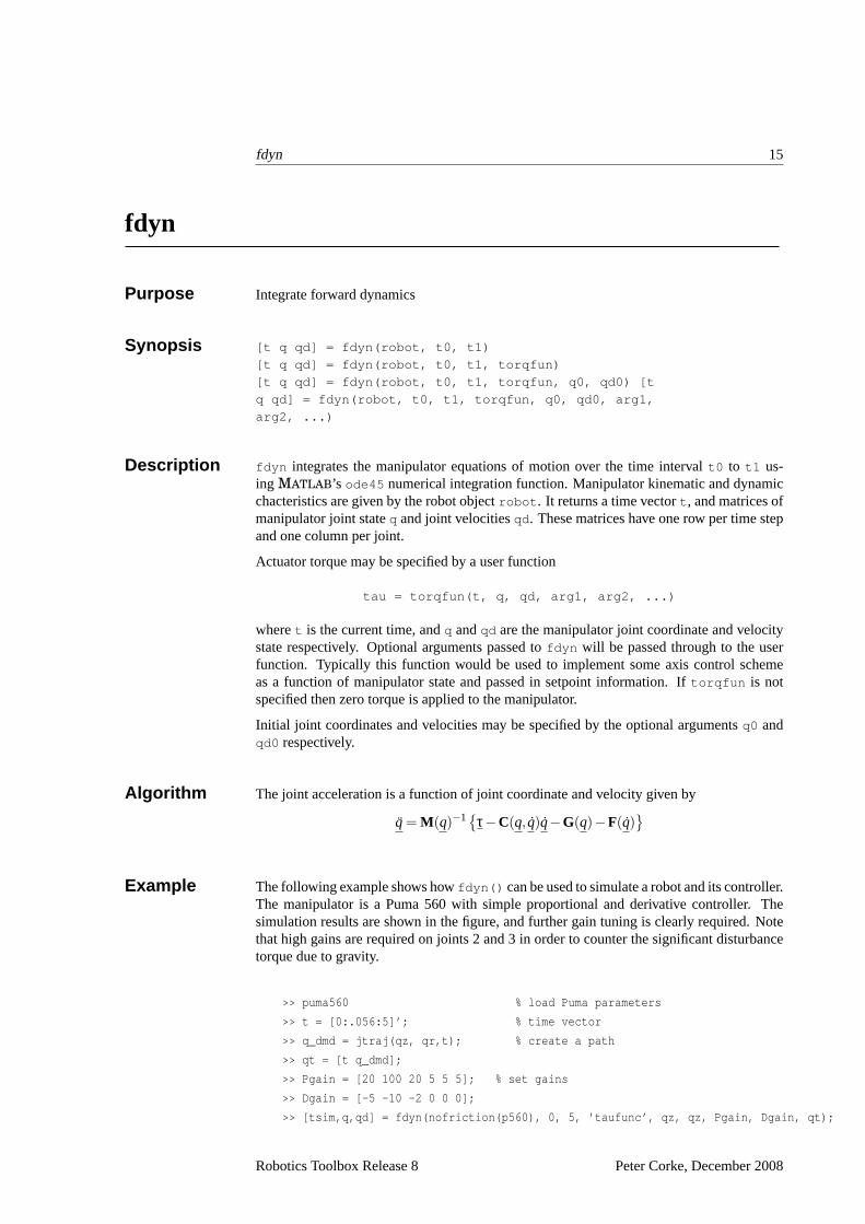
fdyn
Purpose Integrate forward dynamics
Synopsis [t q qd] = fdyn(robot, t0, t1)
[t q qd] = fdyn(robot, t0, t1, torqfun)
[t q qd] = fdyn(robot, t0, t1, torqfun, q0, qd0) [t
q qd] = fdyn(robot, t0, t1, torqfun, q0, qd0, arg1,
arg2, ...)
Description fdyn integrates the manipulator equations of motion over the time intervalt0 to t1 us-ing MATLAB’s ode45 numerical integration function. Manipulator kinematic and dynamicchacteristics are given by the robot objectrobot . It returns a time vectort , and matrices ofmanipulator joint stateq and joint velocitiesqd. These matrices have one row per time stepand one column per joint.
Actuator torque may be specified by a user function
tau = torqfun(t, q, qd, arg1, arg2, ...)
wheret is the current time, andq andqd are the manipulator joint coordinate and velocitystate respectively. Optional arguments passed tofdyn will be passed through to the userfunction. Typically this function would be used to implement some axis control schemeas a function of manipulator state and passed in setpoint information. If torqfun is notspecified then zero torque is applied to the manipulator.
Initial joint coordinates and velocities may be specified bythe optional argumentsq0 andqd0 respectively.
Algorithm The joint acceleration is a function of joint coordinate andvelocity given by
q = M(q)−1
τ−C(q, q)q−G(q)−F(q)
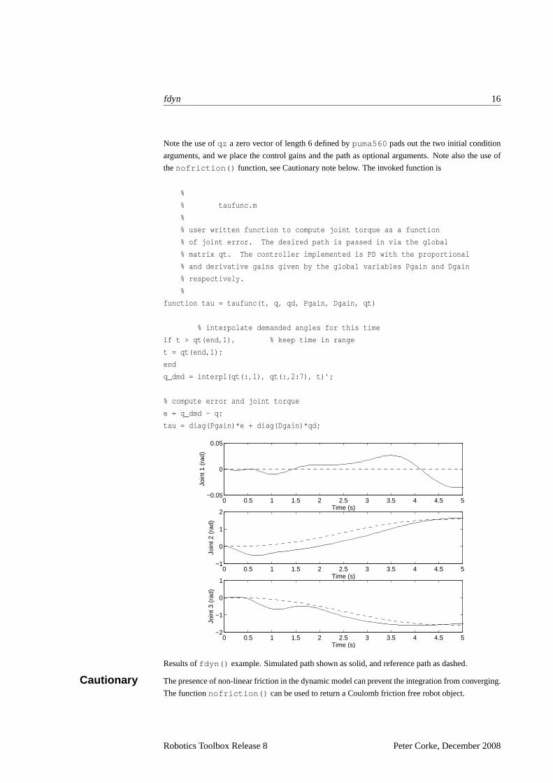
Example The following example shows howfdyn() can be used to simulate a robot and its controller.The manipulator is a Puma 560 with simple proportional and derivative controller. Thesimulation results are shown in the figure, and further gain tuning is clearly required. Notethat high gains are required on joints 2 and 3 in order to counter the significant disturbancetorque due to gravity.
>> puma560 % load Puma parameters
>> t = [0:.056:5]’; % time vector
>> q_dmd = jtraj(qz, qr,t); % create a path
>> qt = [t q_dmd];
>> Pgain = [20 100 20 5 5 5]; % set gains
>> Dgain = [-5 -10 -2 0 0 0];
>> [tsim,q,qd] = fdyn(nofriction(p560), 0, 5, ’taufunc’, q z, qz, Pgain, Dgain, qt);
Robotics Toolbox Release 8 Peter Corke, December 2008
fdyn 16
Note the use ofqz a zero vector of length 6 defined bypuma560 pads out the two initial condition
arguments, and we place the control gains and the path as optional arguments. Note also the use of
thenofriction() function, see Cautionary note below. The invoked function is
%
% taufunc.m
%
% user written function to compute joint torque as a function
% of joint error. The desired path is passed in via the global
% matrix qt. The controller implemented is PD with the propor tional
% and derivative gains given by the global variables Pgain an d Dgain
% respectively.
%
function tau = taufunc(t, q, qd, Pgain, Dgain, qt)
% interpolate demanded angles for this time
if t > qt(end,1), % keep time in range
t = qt(end,1);
end
q_dmd = interp1(qt(:,1), qt(:,2:7), t)’;
% compute error and joint torque
e = q_dmd - q;
tau = diag(Pgain)*e + diag(Dgain)*qd;
0 0.5 1 1.5 2 2.5 3 3.5 4 4.5 5−2
−1
0
1
Time (s)
Join
t 3 (
rad)
0 0.5 1 1.5 2 2.5 3 3.5 4 4.5 5−1
0
1
2
Time (s)
Join
t 2 (
rad)
0 0.5 1 1.5 2 2.5 3 3.5 4 4.5 5−0.05
0
0.05
Time (s)
Join
t 1 (
rad)
Results offdyn() example. Simulated path shown as solid, and reference path as dashed.
Cautionary The presence of non-linear friction in the dynamic model can prevent the integration from converging.
The functionnofriction() can be used to return a Coulomb friction free robot object.
Robotics Toolbox Release 8 Peter Corke, December 2008

fdyn 17
See Also accel, nofriction, rne, robot, ode45
References M. W. Walker and D. E. Orin. Efficient dynamic computer simulation of robotic mechanisms.ASME
Journal of Dynamic Systems, Measurement and Control, 104:205–211, 1982.
Robotics Toolbox Release 8 Peter Corke, December 2008
fkine 18
fkine
Purpose Forward robot kinematics for serial link manipulator
Synopsis T = fkine(robot, q)
Description fkine computes forward kinematics for the joint coordinateq giving a homogeneous transform for
the location of the end-effector.robot is a robot object which contains a kinematic model in either
standard or modified Denavit-Hartenberg notation. Note that the robot object can specify an arbitrary
homogeneous transform for the base of the robot and a tool offset.
If q is a vector it is interpreted as the generalized joint coordinates, andfkine returns a homogeneous
transformation for the final link of the manipulator. Ifq is a matrix each row is interpreted as a joint
state vector, andT is a 4×4×m matrix wheremis the number of rows inq.
Cautionary Note that the dimensional units for the last column of theT matrix will be the same as the dimensional
units used in therobot object. The units can be whatever you choose (metres, inches, cubits or
furlongs) but the choice will affect the numerical value of the elements inthe last column ofT. The
Toolbox definitionspuma560 andstanford all use SI units with dimensions in metres.
See Also link, robot
References R. P. Paul.Robot Manipulators: Mathematics, Programming, and Control. MIT Press, Cambridge,
Massachusetts, 1981.
J. J. Craig,Introduction to Robotics. Addison Wesley, second ed., 1989.
Robotics Toolbox Release 8 Peter Corke, December 2008
link/friction 19
link/friction
Purpose Compute joint friction torque
Synopsis tau f = friction(link, qd)
Description friction computes the joint friction torque based on friction parameter data, if any,in the link
objectlink . Friction is a function only of joint velocityqd
If qd is a vector thentau f is a vector in which each element is the friction torque for the the
corresponding element inqd .
Algorithm The friction model is a fairly standard one comprising viscous friction anddirection dependent
Coulomb friction
Fi(t) =
Bi q+ τ−i , θ < 0
Bi q+ τ+i , θ > 0
See Also link,robot/friction,nofriction
Robotics Toolbox Release 8 Peter Corke, December 2008

robot/friction 20
robot/friction
Purpose Compute robot friction torque vector
Synopsis tau f = friction(robot, qd)
Description friction computes the joint friction torque vector for the robot objectrobot with a joint velocity
vectorqd .
See Also link, link/friction, nofriction
Robotics Toolbox Release 8 Peter Corke, December 2008
ftrans 21
ftrans
Purpose Force transformation
Synopsis F2 = ftrans(F, T)
Description Transform the force vectorF in the current coordinate frame to force vectorF2 in the second coordi-
nate frame. The second frame is related to the first by the homogeneoustransformT. F2 andF are
each 6-element vectors comprising force and moment components[Fx Fy Fz Mx My Mz].
See Also diff2tr
Robotics Toolbox Release 8 Peter Corke, December 2008
gravload 22
gravload
Purpose Compute the manipulator gravity torque components
Synopsis tau g = gravload(robot, q)
tau g = gravload(robot, q, grav)
Description gravload computes the joint torque due to gravity for the manipulator in poseq.
If q is a row vector,tau g returns a row vector of joint torques. Ifq is a matrix each row is interpreted
as as a joint state vector, andtau g is a matrix in which each row is the gravity torque for the the
corresponding row inq.
The default gravity direction comes from the robot object but may be overridden by the optionalgrav
argument.
See Also robot, link, rne, itorque, coriolis
References M. W. Walker and D. E. Orin. Efficient dynamic computer simulation of robotic mechanisms.ASME
Journal of Dynamic Systems, Measurement and Control, 104:205–211, 1982.
Robotics Toolbox Release 8 Peter Corke, December 2008

ikine 23
ikine
Purpose Inverse manipulator kinematics
Synopsis q = ikine(robot, T)
q = ikine(robot, T, q0)
q = ikine(robot, T, q0, M)
Description ikine returns the joint coordinates for the manipulator described by the objectrobot whose end-
effector homogeneous transform is given byT. Note that the robot’s base can be arbitrarily specified
within the robot object.
If T is a homogeneous transform then a row vector of joint coordinates is returned. The estimate for
the first step isq0 if this is given else 0.
If T is a homogeneous transform trajectory of size 4×4×m thenq will be an n×m matrix where
each row is a vector of joint coordinates corresponding to the last subscript of T. The estimate for the
first step in the sequence isq0 if this is given else 0. The initial estimate ofq for each time step is
taken as the solution from the previous time step.
Note that the inverse kinematic solution is generally not unique, and depends on the initial valueq0
(which defaults to 0).
For the case of a manipulator with fewer than 6 DOF it is not possible for the end-effector to satisfy
the end-effector pose specified by an arbitrary homogeneous transform. This typically leads to non-
convergence inikine . A solution is to specify a 6-element weighting vector,M, whose elements
are 0 for those Cartesian DOF that are unconstrained and 1 otherwise. The elements correspond
to translation along the X-, Y- and Z-axes and rotation about the X-, Y- andZ-axes respectively.
For example, a 5-axis manipulator may be incapable of independantly controlling rotation about the
end-effector’s Z-axis. In this caseM = [1 1 1 1 1 0] would enable a solution in which the end-
effector adopted the poseT except for the end-effector rotation. The number of non-zero elements
should equal the number of robot DOF.
Algorithm The solution is computed iteratively using the pseudo-inverse of the manipulator Jacobian.
q = J+(q)∆(
F (q)−T)
where∆ returns the ‘difference’ between two transforms as a 6-element vector of displacements and
rotations (seetr2diff ).
Cautionary Such a solution is completely general, though much less efficient than specific inverse kinematic
solutions derived symbolically.
The returned joint angles may be in non-minimum form, ie.q+2nπ.
This approach allows a solution to obtained at a singularity, but the joint coordinates within the null
space are arbitrarily assigned.
Robotics Toolbox Release 8 Peter Corke, December 2008
ikine 24
Note that the dimensional units used for the last column of theT matrix must agree with the dimen-
sional units used in the robot definition. These units can be whatever you choose (metres, inches,
cubits or furlongs) but they must be consistent. The Toolbox definitionspuma560 andstanford
all use SI units with dimensions in metres.
See Also fkine, tr2diff, jacob0, ikine560, robot
References S. Chieaverini, L. Sciavicco, and B. Siciliano, “Control of robotic systems through singularities,” in
Proc. Int. Workshop on Nonlinear and Adaptive Control: Issues in Robotics (C. C. de Wit, ed.),
Springer-Verlag, 1991.
Robotics Toolbox Release 8 Peter Corke, December 2008
ikine560 25
ikine560
Purpose Inverse manipulator kinematics for Puma 560 like arm
Synopsis q = ikine560(robot, config)
Description ikine560 returns the joint coordinates corresponding to the end-effector homogeneous transform
T. It is computed using a symbolic solution appropriate for Puma 560 like robots, that is, all revolute
6DOF arms, with a spherical wrist. The use of a symbolic solution means that it executes over 50
times faster thanikine for a Puma 560 solution.
A further advantage is thatikine560() allows control over the specific solution returned.config
is a string which contains one or more of the configuration control letter codes
’l’ left-handed (lefty) solution (default)
’r’ †right-handed (righty) solution
’u’ †elbow up solution (default)
’d’ elbow down solution
’f’ †wrist flipped solution
’n’ wrist not flipped solution (default)
Cautionary Note that the dimensional units used for the last column of theT matrix must agree with the dimen-
sional units used in therobot object. These units can be whatever you choose (metres, inches, cubits
or furlongs) but they must be consistent. The Toolbox definitionspuma560 andstanford all use
SI units with dimensions in metres.
See Also fkine, ikine, robot
References R. P. Paul and H. Zhang, “Computationally efficient kinematics for manipulators with spherical
wrists,” Int. J. Robot. Res., vol. 5, no. 2, pp. 32–44, 1986.
Author Robert Biro and Gary McMurray, Georgia Institute of Technology, [email protected]
Robotics Toolbox Release 8 Peter Corke, December 2008
inertia 26
inertia
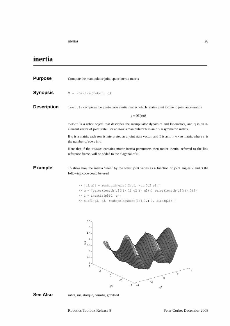
Purpose Compute the manipulator joint-space inertia matrix
Synopsis M = inertia(robot, q)
Description inertia computes the joint-space inertia matrix which relates joint torque to joint acceleration
τ = M(q)q
robot is a robot object that describes the manipulator dynamics and kinematics,and q is an n-
element vector of joint state. For an n-axis manipulatorMis ann×n symmetric matrix.
If q is a matrix each row is interpreted as a joint state vector, andI is ann×n×m matrix wheremis
the number of rows inq.
Note that if therobot contains motor inertia parameters then motor inertia, referred to the link
reference frame, will be added to the diagonal ofM.
Example To show how the inertia ‘seen’ by the waist joint varies as a function of jointangles 2 and 3 the
following code could be used.
>> [q2,q3] = meshgrid(-pi:0.2:pi, -pi:0.2:pi);
>> q = [zeros(length(q2(:)),1) q2(:) q3(:) zeros(length(q 2(:)),3)];
>> I = inertia(p560, q);
>> surfl(q2, q3, reshape(squeeze(I(1,1,:)), size(q2)));
−4−2
02
4
−4
−2
0
2
42
2.5
3
3.5
4
4.5
5
5.5
q2q3
I11
See Also robot, rne, itorque, coriolis, gravload
Robotics Toolbox Release 8 Peter Corke, December 2008

inertia 27
References M. W. Walker and D. E. Orin. Efficient dynamic computer simulation of robotic mechanisms.ASME
Journal of Dynamic Systems, Measurement and Control, 104:205–211, 1982.
Robotics Toolbox Release 8 Peter Corke, December 2008

ishomog 28
ishomog
Purpose Test if argument is a homogeneous transform
Synopsis ishomog(x)
Description Returns true ifx is a 4× 4 matrix.
See Also isrot, isvec
Robotics Toolbox Release 8 Peter Corke, December 2008
isrot 29
isrot
Purpose Test if argument is a rotation matrix
Synopsis isrot(x)
Description Returns true ifx is a 3× 3 matrix.
See Also ishomog, isvec
Robotics Toolbox Release 8 Peter Corke, December 2008

isvec 30
isvec
Purpose Test if argument is a 3-vector
Synopsis isvec(x)
Description Returns true ifx is , either a 3×1 or 1×3 matrix.
See Also ishomog, isrot
Robotics Toolbox Release 8 Peter Corke, December 2008
itorque 31
itorque
Purpose Compute the manipulator inertia torque component
Synopsis tau i = itorque(robot, q, qdd)
Description itorque returns the joint torque due to inertia at the specified poseq and accelerationqdd which is
given by
τi = M(q)q
If q andqdd are row vectors,itorque is a row vector of joint torques. Ifq andqdd are matrices,
each row is interpreted as a joint state vector, anditorque is a matrix in which each row is the
inertia torque for the corresponding rows ofq andqdd .
robot is a robot object that describes the kinematics and dynamics of the manipulator and drive. If
robot contains motor inertia parameters then motor inertia, referred to the link reference frame, will
be included in the diagonal ofMand influence the inertia torque result.
See Also robot, rne, coriolis, inertia, gravload
Robotics Toolbox Release 8 Peter Corke, December 2008
jacob0 32
jacob0
Purpose Compute manipulator Jacobian in base coordinates
Synopsis jacob0(robot, q)
Description jacob0 returns a Jacobian matrix for the robot objectrobot in the poseq and as expressed in the
base coordinate frame.
The manipulator Jacobian matrix,0Jq, maps differential velocities in joint space, ˙q, to Cartesian
velocity of the end-effector expressed in the base coordinate frame.
0x = 0Jq(q)q
For an n-axis manipulator the Jacobian is a 6×n matrix.
See Also jacobn, diff2tr, tr2diff, robot
References R. P. Paul, B. Shimano and G. E. Mayer.Kinematic Control Equations for Simple Manipulators.
IEEE Systems, Man and Cybernetics 11(6), pp 449-455, June 1981.
Robotics Toolbox Release 8 Peter Corke, December 2008
jacobn 33
jacobn
Purpose Compute manipulator Jacobian in end-effector coordinates
Synopsis jacobn(robot, q)
Description jacobn returns a Jacobian matrix for the robot objectrobot in the poseq and as expressed in the
end-effector coordinate frame.
The manipulator Jacobian matrix,0Jq, maps differential velocities in joint space, ˙q, to Cartesian
velocity of the end-effector expressed in the end-effector coordinateframe.
nx = nJq(q)q
The relationship between tool-tip forces and joint torques is given by
τ = nJq(q)′nF
For an n-axis manipulator the Jacobian is a 6×n matrix.
See Also jacob0, diff2tr, tr2diff, robot
References R. P. Paul, B. Shimano and G. E. Mayer.Kinematic Control Equations for Simple Manipulators.
IEEE Systems, Man and Cybernetics 11(6), pp 449-455, June 1981.
Robotics Toolbox Release 8 Peter Corke, December 2008
jtraj 34
jtraj
Purpose Compute a joint space trajectory between two joint coordinate poses
Synopsis [q qd qdd] = jtraj(q0, q1, n)
[q qd qdd] = jtraj(q0, q1, n, qd0, qd1)
[q qd qdd] = jtraj(q0, q1, t)
[q qd qdd] = jtraj(q0, q1, t, qd0, qd1)
Description jtraj returns a joint space trajectoryq from joint coordinatesq0 to q1 . The number of points isn
or the length of the given time vectort . A 7th order polynomial is used with default zero boundary
conditions for velocity and acceleration.
Non-zero boundary velocities can be optionally specified asqd0 andqd1 .
The trajectory is a matrix, with one row per time step, and one column per joint.The function can
optionally return a velocity and acceleration trajectories asqd andqdd respectively.
See Also ctraj
Robotics Toolbox Release 8 Peter Corke, December 2008
link 35
link
Purpose Link object
Synopsis L = link
L = link([alpha, a, theta, d], convention)
L = link([alpha, a, theta, d, sigma], convention)
L = link(dyn row, convention)
A = link(q)
show(L)
Description The link function constructs alink object. The object contains kinematic and dynamic parameters
as well as actuator and transmission parameters. The first form returns a default object, while the
second and third forms initialize the kinematic model based on Denavit and Hartenberg parameters.
The dynamic model can be initialized using the fourth form of the constructor wheredyn row is a
1×20 matrix which is one row of the legacydyn matrix.
By default the standard Denavit and Hartenberg conventions are assumed but this can be overridden
by the optionalconvention argument which can be set to either’modified’ or ’standard’
(default). Note that any abbreviation of the string can be used, ie.’mod’ or even’m’ .
The second last form given above is not a constructor but a link methodthat returns the link transfor-
mation matrix for the given joint coordinate. The argument is given to the link object using paren-
thesis. The single argument is taken as the link variableq and substituted forθ or D for a revolute or
prismatic link respectively.
The Denavit and Hartenberg parameters describe the spatial relationship between this link and the pre-
vious one. The meaning of the fields for each kinematic convention are summarized in the following
table.
variable DH MDH description
alpha αi αi−1 link twist angle
A Ai Ai−1 link length
theta θi θi link rotation angle
D Di Di link offset distance
sigma σi σi joint type; 0 for revolute, non-zero for prismatic
Since Matlab does not support the concept of public class variables methods have been written to
allow link object parameters to be referenced (r) or assigned (a) as given by the following table
Robotics Toolbox Release 8 Peter Corke, December 2008
link 36
Method Operations Returns
link .alpha r+a link twist angle
link .A r+a link length
link .theta r+a link rotation angle
link .D r+a link offset distance
link .sigma r+a joint type; 0 for revolute, non-zero for prismatic
link .RP r joint type; ’R’ or ’P’
link .mdh r+a DH convention: 0 if standard, 1 if modified
link .I r 3×3 symmetric inertia matrix
link .I a assigned from a 3×3 matrix or a 6-element vec-
tor interpretted as[Ixx Iyy Izz Ixy Iyz Ixz]
link .m r+a link mass
link .r r+a 3×1 link COG vector
link .G r+a gear ratio
link .Jm r+a motor inertia
link .B r+a viscous friction
link .Tc r Coulomb friction, 1×2 vector where[τ+ τ−]
link .Tc a Coulomb friction; for symmetric friction this is
a scalar, for asymmetric friction it is a 2-element
vector for positive and negative velocity
link .dh r+a row of legacy DH matrix
link .dyn r+a row of legacy DYN matrix
link .qlim r+a joint coordinate limits, 2-vector
link .islimit(q) r return true if value ofq is outside the joint limit
bounds
link .offset r+a joint coordinate offset (see discussion for
robot object).
The default is for standard Denavit-Hartenberg conventions, zero friction, mass and inertias.
The display method gives a one-line summary of the link’s kinematic parameters. Theshow
method displays as many link parameters as have been initialized for that link.
Examples
>> L = link([-pi/2, 0.02, 0, 0.15])
L =
-1.570796 0.020000 0.000000 0.150000 R (std)
>> L.RP
ans =
R
>> L.mdh
ans =
0
>> L.G = 100;
>> L.Tc = 5;
>> L
Robotics Toolbox Release 8 Peter Corke, December 2008
link 37
L =
-1.570796 0.020000 0.000000 0.150000 R (std)
>> show(L)
alpha = -1.5708
A = 0.02
theta = 0
D = 0.15
sigma = 0
mdh = 0
G = 100
Tc = 5 -5
>>
Algorithm For the standard Denavit-Hartenberg conventions the homogeneous transform
i−1Ai =
cosθi −sinθi cosαi sinθi sinαi ai cosθi
sinθi cosθi cosαi −cosθi sinαi ai sinθi
0 sinαi cosαi di
0 0 0 1
represents each link’s coordinate frame with respect to the previous link’s coordinate system. For a
revolute jointθi is offset by
For the modified Denavit-Hartenberg conventions it is instead
i−1Ai =
cosθi −sinθi 0 ai−1
sinθi cosαi−1 cosθi cosαi−1 −sinαi−1 −di sinαi−1
sinθi sinαi−1 cosθi sinαi−1 cosαi−1 di cosαi−1
0 0 0 1
See Also showlink, robot
References R. P. Paul.Robot Manipulators: Mathematics, Programming, and Control. MIT Press, Cambridge,
Massachusetts, 1981.
J. J. Craig,Introduction to Robotics. Addison Wesley, second ed., 1989.
Robotics Toolbox Release 8 Peter Corke, December 2008
maniplty 38
maniplty
Purpose Manipulability measure
Synopsis m = maniplty(robot, q)
m = maniplty(robot, q, which)
Description maniplty computes the scalar manipulability index for the manipulator at the given pose. Manipu-
lability varies from 0 (bad) to 1 (good).robot is a robot object that contains kinematic and optionally
dynamic parameters for the manipulator. Two measures are supportedand are selected by the optional
argumentwhich can be either’yoshikawa’ (default) or’asada’ . Yoshikawa’s manipulability
measure is based purely on kinematic data, and gives an indication of how‘far’ the manipulator is
from singularities and thus able to move and exert forces uniformly in all directions.
Asada’s manipulability measure utilizes manipulator dynamic data, and indicates how close the inertia
ellipsoid is to spherical.
If q is a vectormaniplty returns a scalar manipulability index. Ifq is a matrixmaniplty returns
a column vector and each row is the manipulability index for the pose specified by the corresponding
row of q.
Algorithm Yoshikawa’s measure is based on the condition number of the manipulatorJacobian
ηyoshi =√
|J(q)J(q)′|
Asada’s measure is computed from the Cartesian inertia matrix
M(x) = J(q)−T M(q)J(q)−1
The Cartesian manipulator inertia ellipsoid is
x′M(x)x = 1
and gives an indication of how well the manipulator can accelerate in each of the Cartesian directions.
The scalar measure computed here is the ratio of the smallest/largest ellipsoid axes
ηasada =minxmaxx
Ideally the ellipsoid would be spherical, giving a ratio of 1, but in practice willbe less than 1.
See Also jacob0, inertia,robot
References T. Yoshikawa, “Analysis and control of robot manipulators with redundancy,” inProc. 1st Int. Symp.
Robotics Research, (Bretton Woods, NH), pp. 735–747, 1983.
Robotics Toolbox Release 8 Peter Corke, December 2008
MotomanHP6 39
MotomanHP6
Purpose Create a Motoman HP 6 robot object
Synopsis MotomanHP6
Description Creates therobot objectRwhich describes the kinematic characteristics of a Motoman HP6 manipu-
lator. The kinematic conventions used are as per Paul and Zhang, and all quantities are in standard SI
units.
Also defined is the joint coordinate vectorq0 corresponding to the zero position.
See Also robot, puma560akb, stanford, Fanuc10L, S4ABB2p8
Author Wynand Swart, Mega Robots CC, P/O Box 8412, Pretoria, 0001, South Africa,
Robotics Toolbox Release 8 Peter Corke, December 2008
robot/nofriction 40
robot/nofriction
Purpose Remove friction from robot object
Synopsis robot2 = nofriction(robot)
robot2 = nofriction(robot, ’all’)
Description Return a new robot object with modified joint friction properties. The firstform sets the Coulomb
friction values to zero in the constituent links The second form sets viscousand Coulomb friction
values in the constituent links are set to zero.
The resulting robot object has its name string prepended with ’NF/’.
This is important for forward dynamics computation (fdyn() ) where the presence of friction can
prevent the numerical integration from converging.
See Also link/nofriction, robot, link, friction, fdyn
Robotics Toolbox Release 8 Peter Corke, December 2008

link/nofriction 41
link/nofriction
Purpose Remove friction from link object
Synopsis link2 = nofriction(link)
link2 = nofriction(link, ’all’)
Description Return a new link object with modified joint friction properties. The first form sets the Coulomb
friction values to zero. The second form sets both viscous and Coulomb friction values to zero.
This is important for forward dynamics computation (fdyn() ) where the presence of friction can
prevent the numerical integration from converging.
See Also robot/nofriction, link, friction, fdyn
Robotics Toolbox Release 8 Peter Corke, December 2008
oa2tr, oa2r 42
oa2tr, oa2r
Purpose Convert OA vectors to homogeneous transform or rotation matrix
Synopsis T = oa2tr(o, a)
R = oa2r(o, a)
Description Returns a homogeneous transform or rotation matrix specified in terms ofthe Cartesian orientation
and approach vectorso anda respectively.
AlgorithmR =
[
o× a o a]
where ˆo anda are unit vectors corresponding too anda respectively.
Cautionary An extra cross-product is used to ensure orthonormality.a is the only column that is guaranteed to be
unchanged from that specified in the call.
See Also rpy2tr, eul2tr
Robotics Toolbox Release 8 Peter Corke, December 2008
perturb 43
perturb
Purpose Perturb robot dynamic parameters
Synopsis robot2 = perturb(robot, p)
Description Return a new robot object with randomly modified dynamic parameters: link mass and inertia. The
perturbation is multiplicative so that values are multiplied by random numbersin the interval (1-p) to
(1+p).
Useful for investigating the robustness of various model-based control schemes where one model
forms the basis of the model-based controller and the peturbed model is used for the actual plant.
The resulting robot object has its name string prepended with ’P/’.
See Also fdyn, rne, robot
Robotics Toolbox Release 8 Peter Corke, December 2008
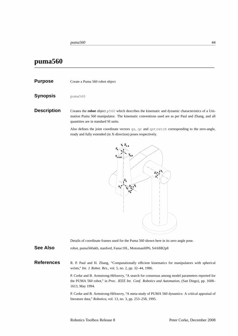
puma560 44
puma560
Purpose Create a Puma 560 robot object
Synopsis puma560
Description Creates therobot objectp560 which describes the kinematic and dynamic characteristics of a Uni-
mation Puma 560 manipulator. The kinematic conventions used are as per Paul and Zhang, and all
quantities are in standard SI units.
Also defines the joint coordinate vectorsqz , qr andqstretch corresponding to the zero-angle,
ready and fully extended (in X-direction) poses respectively.
Details of coordinate frames used for the Puma 560 shown here in its zeroangle pose.
See Also robot, puma560akb, stanford, Fanuc10L, MotomanHP6, S4ABB2p8
References R. P. Paul and H. Zhang, “Computationally efficient kinematics for manipulators with spherical
wrists,” Int. J. Robot. Res., vol. 5, no. 2, pp. 32–44, 1986.
P. Corke and B. Armstrong-Helouvry, “A search for consensus among model parameters reported for
the PUMA 560 robot,” inProc. IEEE Int. Conf. Robotics and Automation, (San Diego), pp. 1608–
1613, May 1994.
P. Corke and B. Armstrong-Helouvry, “A meta-study of PUMA 560 dynamics: A critical appraisal of
literature data,”Robotica, vol. 13, no. 3, pp. 253–258, 1995.
Robotics Toolbox Release 8 Peter Corke, December 2008
puma560akb 45
puma560akb
Purpose Create a Puma 560 robot object
Synopsis puma560akb
Description Creates therobot objectp560m which describes the kinematic and dynamic characteristics of a Uni-
mation Puma 560 manipulator. It uses Craig’s modified Denavit-Hartenberg notation with the partic-
ular kinematic conventions from Armstrong, Khatib and Burdick. All quantities are in standard SI
units.
Also defines the joint coordinate vectorsqz , qr andqstretch corresponding to the zero-angle,
ready and fully extended (in X-direction) poses respectively.
See Also robot, puma560, stanford, Fanuc10L, MotomanHP6, S4ABB2p8
References B. Armstrong, O. Khatib, and J. Burdick, “The explicit dynamic model and inertial parameters of
the Puma 560 arm,” inProc. IEEE Int. Conf. Robotics and Automation, vol. 1, (Washington, USA),
pp. 510–18, 1986.
Robotics Toolbox Release 8 Peter Corke, December 2008
qinterp 46
qinterp
Purpose Interpolate unit-quaternions
Synopsis QI = qinterp(Q1, Q2, r)
Description Return a unit-quaternion that interpolates between Q1 and Q2 asr varies between 0 and 1 inclusively.
This is a spherical linear interpolation (slerp) that can be interpreted as interpolation along a great
circle arc on a sphere.
If r is a vector, then a cell array of quaternions is returned correspondingto successive values ofr .
Examples A simple example
>> q1 = quaternion(rotx(0.3))
q1 =
0.98877 <0.14944, 0, 0>
>> q2 = quaternion(roty(-0.5))
q2 =
0.96891 <0, -0.2474, 0>
>> qinterp(q1, q2, 0)
ans =
0.98877 <0.14944, 0, 0>
>> qinterp(q1, q2, 1)
ans =
0.96891 <0, -0.2474, 0>
>> qinterp(q1, q2, 0.3)
ans =
0.99159 <0.10536, -0.075182, 0>
>>
References K. Shoemake, “Animating rotation with quaternion curves.,” inProceedings of ACM SIGGRAPH,
(San Francisco), pp. 245–254, The Singer Company, Link Flight Simulator Division, 1985.
Robotics Toolbox Release 8 Peter Corke, December 2008
quaternion 47
quaternion
Purpose Quaternion object
Synopsis q = quaternion(qq)
q = quaternion(v, theta)
q = quaternion(R)
q = quaternion([s vx vy vz])
Description quaternion is the constructor for aquaternion object. The first form returns a new object with the
same value as its argument. The second form initializes the quaternion to a rotation of theta about
the vectorv .
Examples A simple example
>> quaternion(1, [1 0 0])
ans =
0.87758 <0.47943, 0, 0>
>> quaternion( rotx(1) )
ans =
0.87758 <0.47943, 0, 0>
>>
The third form sets the quaternion to a rotation equivalent to the given 3×3 rotation matrix, or the
rotation submatrix of a 4×4 homogeneous transform.
The fourth form sets the four quaternion elements directly wheres is the scalar component and[vx
vy vz] the vector.
All forms, except the last, return a unit quaternion, ie. one whose magnitude is unity.
Some operators are overloaded for the quaternion class
Robotics Toolbox Release 8 Peter Corke, December 2008
quaternion 48
q1 + q2 returns the elementwise sum of quaternion elements
q1 - q2 returns he elementwise sum of quaternion elements
q1 * q2 returns quaternion product or compounding
q * v returns a quaternion vector product, that is the vectorv is rotated
by the quaternion.v is a 3×3 vector
q1 / q2 returnsq1 ∗q−12
q∧j returnsq j where j is an integer exponent. Forj > 0 the result
is obtained by repeated multiplication. Forj < 0 the final result
is inverted.
double(q) returns the quaternion coeffients as a 4-element row vector
inv(q) returns the quaterion inverse
norm(q) returns the quaterion magnitude
plot(q) displays a 3D plot showing the standard coordinate frame after
rotation byq.
unit(q) returns the corresponding unit quaterion
Some public class variables methods are also available for reference only.
method Returns
quaternion .d return 4-vector of quaternion elements
quaternion .s return scalar component
quaternion .v return vector component
quaternion .t return equivalent homogeneous transformation
matrix
quaternion .r return equivalent orthonormal rotation matrix
Examples
>> t = rotx(0.2)
t =
1.0000 0 0 0
0 0.9801 -0.1987 0
0 0.1987 0.9801 0
0 0 0 1.0000
>> q1 = quaternion(t)
q1 =
0.995 <0.099833, 0, 0>
>> q1.r
ans =
1.0000 0 0
0 0.9801 -0.1987
0 0.1987 0.9801
>> q2 = quaternion( roty(0.3) )
q2 =
0.98877 <0, 0.14944, 0>
Robotics Toolbox Release 8 Peter Corke, December 2008
quaternion 49
>> q1 * q2
ans =
0.98383 <0.098712, 0.14869, 0.014919>
>> q1*q1
ans =
0.98007 <0.19867, 0, 0>
>> q1ˆ2
ans =
0.98007 <0.19867, 0, 0>
>> q1*inv(q1)
ans =
1 <0, 0, 0>
>> q1/q1
ans =
1 <0, 0, 0>
>> q1/q2
ans =
0.98383 <0.098712, -0.14869, -0.014919>
>> q1*q2ˆ-1
ans =
0.98383 <0.098712, -0.14869, -0.014919>
Cautionary At the moment vectors or arrays of quaternions are not supported. You can however use cell arrays to
hold a number of quaternions.
See Also quaternion/plot
References K. Shoemake, “Animating rotation with quaternion curves.,” inProceedings of ACM SIGGRAPH,
(San Francisco), pp. 245–254, The Singer Company, Link Flight Simulator Division, 1985.
Robotics Toolbox Release 8 Peter Corke, December 2008
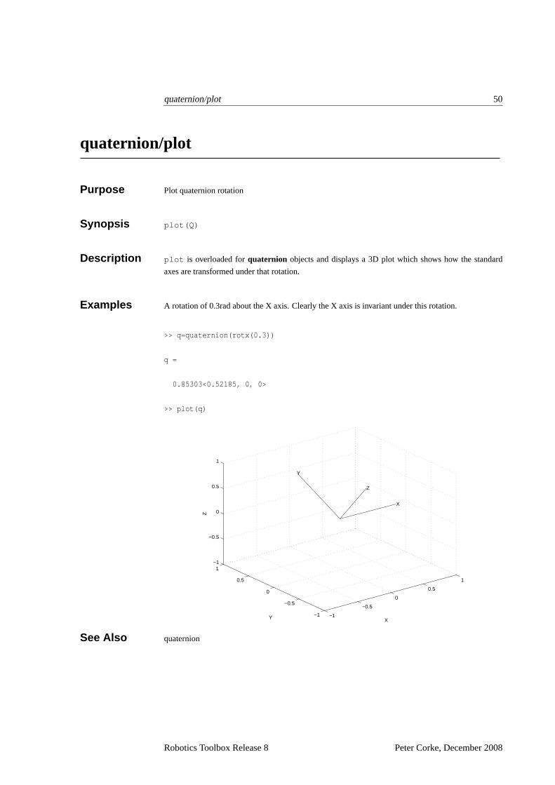
quaternion/plot 50
quaternion/plot
Purpose Plot quaternion rotation
Synopsis plot(Q)
Description plot is overloaded forquaternion objects and displays a 3D plot which shows how the standard
axes are transformed under that rotation.
Examples A rotation of 0.3rad about the X axis. Clearly the X axis is invariant under this rotation.
>> q=quaternion(rotx(0.3))
q =
0.85303<0.52185, 0, 0>
>> plot(q)
−1
−0.5
0
0.5
1
−1
−0.5
0
0.5
1−1
−0.5
0
0.5
1
X
X
Z
Y
Y
Z
See Also quaternion
Robotics Toolbox Release 8 Peter Corke, December 2008
rne 51
rne
Purpose Compute inverse dynamics via recursive Newton-Euler formulation
Synopsis tau = rne(robot, q, qd, qdd)
tau = rne(robot, [q qd qdd])
tau = rne(robot, q, qd, qdd, grav)
tau = rne(robot, [q qd qdd], grav)
tau = rne(robot, q, qd, qdd, grav, fext)
tau = rne(robot, [q qd qdd], grav, fext)
Description rne computes the equations of motion in an efficient manner, giving joint torque as a function of joint
position, velocity and acceleration.
If q, qd andqdd are row vectors thentau is a row vector of joint torques. Ifq, qd andqdd are
matrices thentau is a matrix in which each row is the joint torque for the corresponding rows of q,
qd andqdd .
Gravity direction is defined by the robot object but may be overridden byproviding a gravity acceler-
ation vectorgrav = [gx gy gz] .
An external force/moment acting on the end of the manipulator may also bespecified by a 6-element
vectorfext = [Fx Fy Fz Mx My Mz] in the end-effector coordinate frame.
The torque computed may contain contributions due to armature inertia and joint friction if these are
specified in the parameter matrixdyn .
The MEX-file version of this function is over 1000 times faster than the M-file. See Section 1 of this
manual for information about how to compile and install the MEX-file.
Algorithm Coumputes the joint torque
τ = M(q)q+C(q, q)q+F(q)+G(q)
whereM is the manipulator inertia matrix,C is the Coriolis and centripetal torque,F the viscous and
Coulomb friction, andG the gravity load.
Cautionary The MEX file currently ignores support base and tool transforms.
See Also robot, fdyn, accel, gravload, inertia, friction
Limitations A MEX file is currently only available for Sparc architecture.
Robotics Toolbox Release 8 Peter Corke, December 2008

rne 52
References J. Y. S. Luh, M. W. Walker, and R. P. C. Paul. On-line computational scheme for mechanical manip-
ulators.ASME Journal of Dynamic Systems, Measurement and Control, 102:69–76, 1980.
Robotics Toolbox Release 8 Peter Corke, December 2008
robot 53
robot
Purpose Robot object
Synopsis r = robot
r = robot(rr)
r = robot(link ...)
r = robot(DH ...)
r = robot(DYN ...)
Description robot is the constructor for a robot object. The first form creates a default robot, and the second
form returns a new robot object with the same value as its argument. The third form creates a robot
from a cell array of link objects which define the robot’s kinematics and optionally dynamics. The
fourth and fifth forms create a robot object from legacy DH and DYN format matrices.
The last three forms all accept optional trailing string arguments which are taken in order as being
robot name, manufacturer and comment.
Since Matlab does not support the concept of public class variables methods have been written to
allow robot object parameters to be referenced (r) or assigned (a) as given by the following table
method Operation Returns
robot .n r number of joints
robot .link r+a cell array of link objects
robot .name r+a robot name string
robot .manuf r+a robot manufacturer string
robot .comment r+a general comment string
robot .gravity r+a 3-element vector defining gravity direction
robot .mdh r DH convention: 0 if standard, 1 if modified.
Determined from the link objects.
robot .base r+a homogeneous transform defining base of robot
robot .tool r+a homogeneous transform defining tool of robot
robot .dh r legacy DH matrix
robot .dyn r legacy DYN matrix
robot .q r+a joint coordinates
robot .qlim r+a joint coordinate limits,n×2 matrix
robot .islimit r joint limit vector, for each joint set to -1, 0 or
1 depending if below low limit, OK, or greater
than upper limit
robot .offset r+a joint coordinate offsets
robot .plotopt r+a options forplot()
robot .lineopt r+a line style for robot graphical links
robot .shadowopt r+a line style for robot shadow links
robot .handle r+a graphics handles
Some of these operations at the robot level are actually wrappers around similarly named link object
Robotics Toolbox Release 8 Peter Corke, December 2008
robot 54
functions:offset , qlim , islimit .
The offset vector is added to the user specified joint angles before anykinematic or dynamic function is
invoked (it is actually implemented within the link object). Similarly it is subtracted after an operation
such as inverse kinematics. The need for a joint offset vector arises because of the constraints of
the Denavit-Hartenberg (or modified Denavit-Hartenberg) notation. Thepose of the robot with zero
joint angles is frequently some rather unusual (or even unachievable)pose. The joint coordinate offset
provides a means to make an arbitrary pose correspond to the zero jointangle case.
Default values for robot parameters are:
robot.name ’noname’
robot.manuf ”
robot.comment ”
robot.gravity [009.81]m/s2
robot.offset ones(n,1)
robot.base eye(4,4)
robot.tool eye(4,4)
robot.lineopt ’Color’, ’black’, ’Linewidth’, 4
robot.shadowopt ’Color’, ’black’, ’Linewidth’, 1
The multiplication operator,* , is overloaded and the product of two robot objects is a robot which is
the series connection of the multiplicands. Tool transforms of all but the last robot are ignored, base
transform of all but the first robot are ignored.
Theplot function is also overloaded and is used to provide a robot animation.
Examples
>> L1 = link([ pi/2 0 0 0])
L =
[1x1 link]
>> L2 = link([ 0 0 0.5 0])
L =
[1x1 link] [1x1 link]
>> r = robot(L)
r =
(2 axis, RR)
grav = [0.00 0.00 9.81]
standard D&H parameters
alpha A theta D R/P
1.570796 0.000000 0.000000 0.000000 R (std)
0.000000 0.000000 0.500000 0.000000 R (std)
Robotics Toolbox Release 8 Peter Corke, December 2008

robot 55
>>
See Also link,plot
Robotics Toolbox Release 8 Peter Corke, December 2008
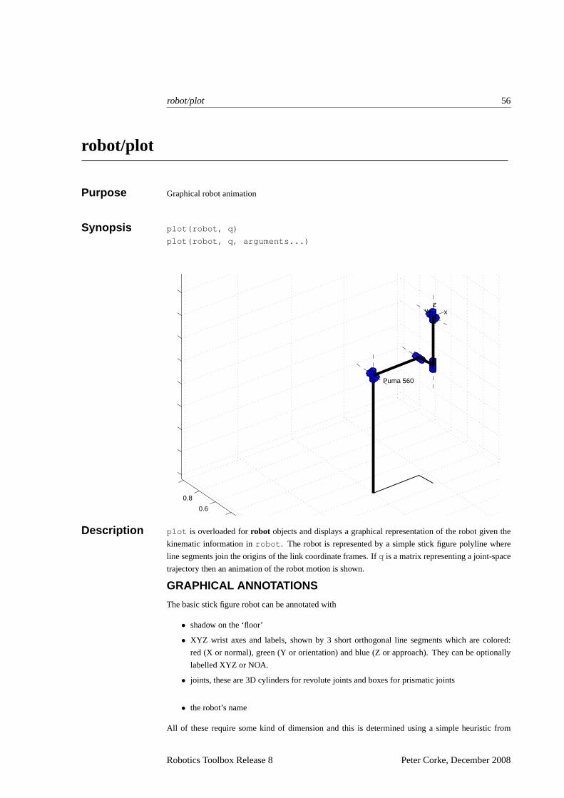
robot/plot 56
robot/plot
Purpose Graphical robot animation
Synopsis plot(robot, q)
plot(robot, q, arguments...)
0.4
0.6
0.8
1
−1
−0.8
−0.6
−0.4
−0.2
0
0.2
0.4
0.6
Puma 560
xyz
Description plot is overloaded forrobot objects and displays a graphical representation of the robot given the
kinematic information inrobot . The robot is represented by a simple stick figure polyline where
line segments join the origins of the link coordinate frames. Ifq is a matrix representing a joint-space
trajectory then an animation of the robot motion is shown.
GRAPHICAL ANNOTATIONS
The basic stick figure robot can be annotated with
• shadow on the ‘floor’
• XYZ wrist axes and labels, shown by 3 short orthogonal line segments which are colored:
red (X or normal), green (Y or orientation) and blue (Z or approach).They can be optionally
labelled XYZ or NOA.
• joints, these are 3D cylinders for revolute joints and boxes for prismatic joints
• the robot’s name
All of these require some kind of dimension and this is determined using a simple heuristic from
Robotics Toolbox Release 8 Peter Corke, December 2008

robot/plot 57
the workspace dimensions. This dimension can be changed by setting the multiplicative scale factor
using themagoption below. These various annotations do slow the rate at which animationswill be
rendered.
OPTIONS
Options are specified by a variable length argument list comprising stringsand numeric values. The
allowed values are:
workspace w set the 3D plot bounds or workspace to the matrix[xmin xmax ymin ymax
zmin zmax]
perspective show a perspective view
ortho show an orthogonal view
base, nobase control display of base, a line from the floor upto joint 0
wrist, nowrist control display of wrist axes
name, noname control display of robot name near joint 0
shadow, noshadow control display of a ’shadow’ on the floor
joints, nojoints control display of joints, these are cylinders for revolute joints and boxesfor
prismatic joints
xyz wrist axis labels are X, Y, Z
noa wrist axis labels are N, O, A
mag scale annotation scale factor
erase, noerase control erasure of robot after each change
loop, noloop control whether animation is repeated endlessly
The options come from 3 sources and are processed in the order:
1. Cell array of options returned by the functionPLOTBOTOPTif found on the user’s current
path.
2. Cell array of options returned by the.plotopt method of therobot object. These are set
by the.plotopt method.
3. List of arguments in the command line.
GETTING GRAPHICAL ROBOT STATE
Each graphical robot has a unique tag set equal to the robot’s name. Whenplot is called it looks for
all graphical objects with that name and moves them. The graphical robot holds a copy of therobot
object asUserData . That copy contains the graphical handles of all the graphical sub-elements of
the robot and also the current joint angle state.
This state is used, and adjusted, by thedrivebot function. The current joint angle state can be
obtained byq = plot(robot) . If multiple instances exist, that of the first one returned byfind-
obj() is given.
Examples To animate two Pumas moving in the same figure window.
>> clf
>> p560b = p560; % duplicate the robot
>> p560b.name = ’Another Puma 560’; % give it a unique name
>> p560b.base = transl([-.05 0.5 0]); % move its base
Robotics Toolbox Release 8 Peter Corke, December 2008
robot/plot 58
>> plot(p560, qr); % display it at ready position
>> hold on
>> plot(p560b, qr); % display it at ready position
>> t = [0:0.056:10];
>> jt = jtraj(qr, qstretch, t); % trajectory to stretch pose
>> for q = jt’, % for all points on the path
>> plot(p560, q);
>> plot(p560b, q);
>> end
To show multiple views of the same robot.
>> clf
>> figure % create a new figure
>> plot(p560, qz); % add a graphical robot
>> figure % create another figure
>> plot(p560, qz); % add a graphical robot
>> plot(p560, qr); % both robots should move
Now the two figures can be adjusted to give different viewpoints, for instance, plan and elevation.
Cautionary plot() options are only processed on the first call when the graphical object isestablished, they are
skipped on subsequent calls. Thus if you wish to change options, clear the figure before replotting.
See Also drivebot, fkine, robot
Robotics Toolbox Release 8 Peter Corke, December 2008
rotx, roty, rotz 59
rotx, roty, rotz
Purpose Rotation about X, Y or Z axis
Synopsis R = rotx(theta)
R = roty(theta)
R = rotz(theta)
Description Return a rotation matrix representing a rotation oftheta radians about the X, Y or Z axes.
See Also rotvec
Robotics Toolbox Release 8 Peter Corke, December 2008
rpy2tr, rpy2r 60
rpy2tr, rpy2r
Purpose Roll/pitch/yaw angles to homogeneous transform or rotation matrix
Synopsis T = rpy2tr([r p y])
T = rpy2tr(r,p,y)
R = rpy2r([r p y])
R = rpy2r(r,p,y)
Description Returns a homogeneous transform or rotation matrix for the specified roll/pitch/yaw angles in radians.
RX (r)RY (p)RZ(y)
For the homogeneous transform value the translational component is set to zero.
See Also tr2rpy, eul2tr
References R. P. Paul,Robot Manipulators: Mathematics, Programming, and Control. Cambridge, Mas-
sachusetts: MIT Press, 1981.
Robotics Toolbox Release 8 Peter Corke, December 2008
rtdemo 61
rtdemo
Purpose Robot Toolbox demonstration
Synopsis rtdemo
Description This script provides demonstrations for most functions within the RoboticsToolbox. It pops up a
graphical menu of demos which will run in the command window. The demos display tutorial infor-
mation and require the user to hit the enter key to display the next pageful of text.
Demos can also be accessed throughMATLAB’s own demo system, using thedemos command or
the command menu option. Then the user can navigate to the Robot Toolboxdemo menu.
Cautionary This script clears all variables in the workspace and deletes all figures.It also adds thedemos direc-
tory to yourMATLAB path on first invocation.
Robotics Toolbox Release 8 Peter Corke, December 2008
S4ABB2p8 62
S4ABB2p8
Purpose Create a Motoman HP 6 robot object
Synopsis S4ABB2p8
Description Creates therobot objectRwhich describes the kinematic characteristics of an ABB S4 2.8 manipula-
tor. The kinematic conventions used are as per Paul and Zhang, and allquantities are in standard SI
units.
Also defined is the joint coordinate vectorq0 corresponding to the synchronization position.
See Also robot, puma560akb, stanford, Fanuc10L, MotomanHP6
Author Wynand Swart, Mega Robots CC, P/O Box 8412, Pretoria, 0001, South Africa,
Robotics Toolbox Release 8 Peter Corke, December 2008
showlink 63
showlink
Purpose Show robot link details
Synopsis showlink(robot)
showlink(link)
Description Displays in detail all the parameters, including all defined inertial parameters, of a link. The first form
provides this level of detail for all links in the specified manipulator. roll/pitch/yaw angles in radians.
Examples To show details of Puma link 2
>> showlink(p560.link2)
alpha = 0
A = 0.4318
theta = 0
D = 0
sigma = 0
mdh = 0
offset = 0
m = 17.4
r = -0.3638
0.006
0.2275
I = 0.13 0 0
0 0.524 0
0 0 0.539
Jm = 0.0002
G = 107.815
B = 0.000817
Tc = 0.126 -0.071
qlim =
>>
Robotics Toolbox Release 8 Peter Corke, December 2008
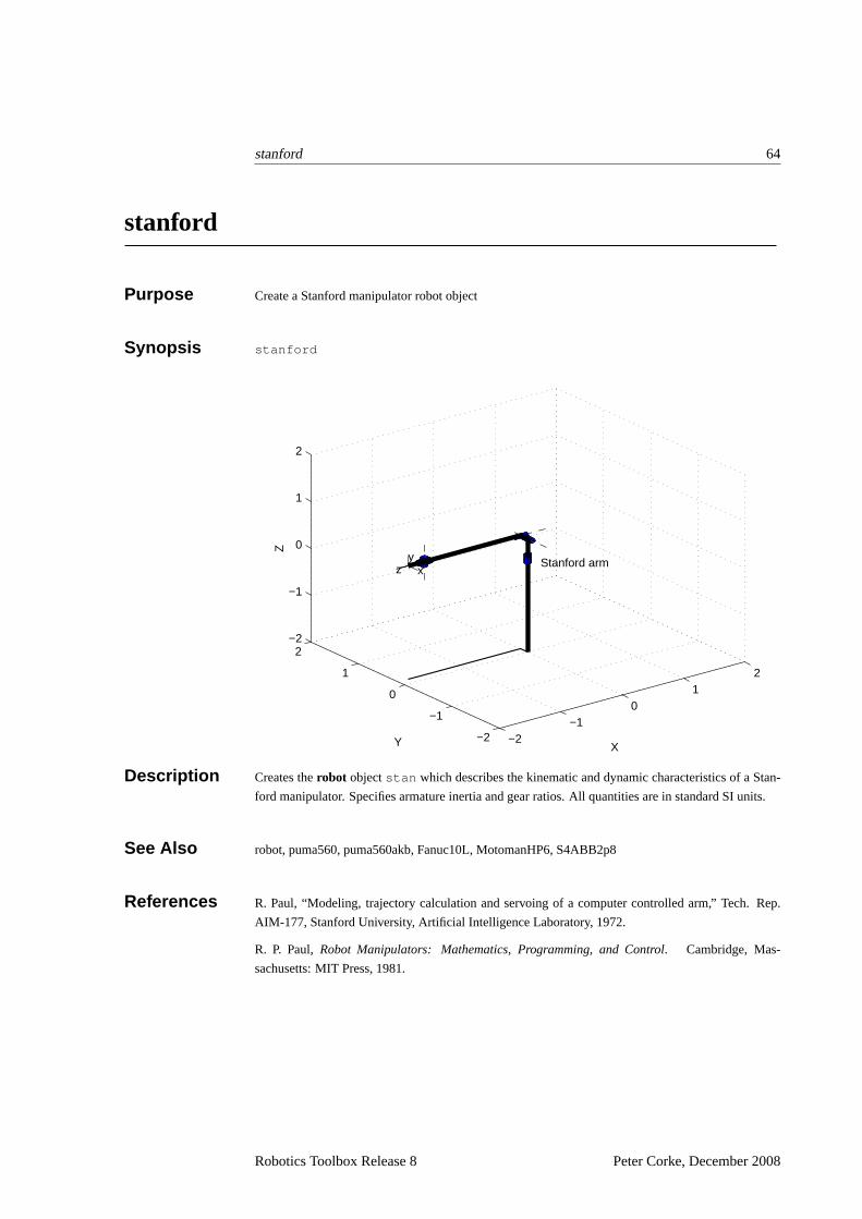
stanford 64
stanford
Purpose Create a Stanford manipulator robot object
Synopsis stanford
−2−1
01
2
−2
−1
0
1
2−2
−1
0
1
2
XY
Z
Stanford armx
yz
Description Creates therobot objectstan which describes the kinematic and dynamic characteristics of a Stan-
ford manipulator. Specifies armature inertia and gear ratios. All quantitiesare in standard SI units.
See Also robot, puma560, puma560akb, Fanuc10L, MotomanHP6, S4ABB2p8
References R. Paul, “Modeling, trajectory calculation and servoing of a computer controlled arm,” Tech. Rep.
AIM-177, Stanford University, Artificial Intelligence Laboratory, 1972.
R. P. Paul,Robot Manipulators: Mathematics, Programming, and Control. Cambridge, Mas-
sachusetts: MIT Press, 1981.
Robotics Toolbox Release 8 Peter Corke, December 2008
tr2angvec 65
tr2angvec
Purpose Convert a homogeneous transform or rotation matrix to angle/vector form
Synopsis [theta, v] = tr2angvec(T)
Description Converts a homogeneous transform or rotation matrix to a rotation oftheta radians about the vector
v .
See Also rotx, roty, rotz
Robotics Toolbox Release 8 Peter Corke, December 2008
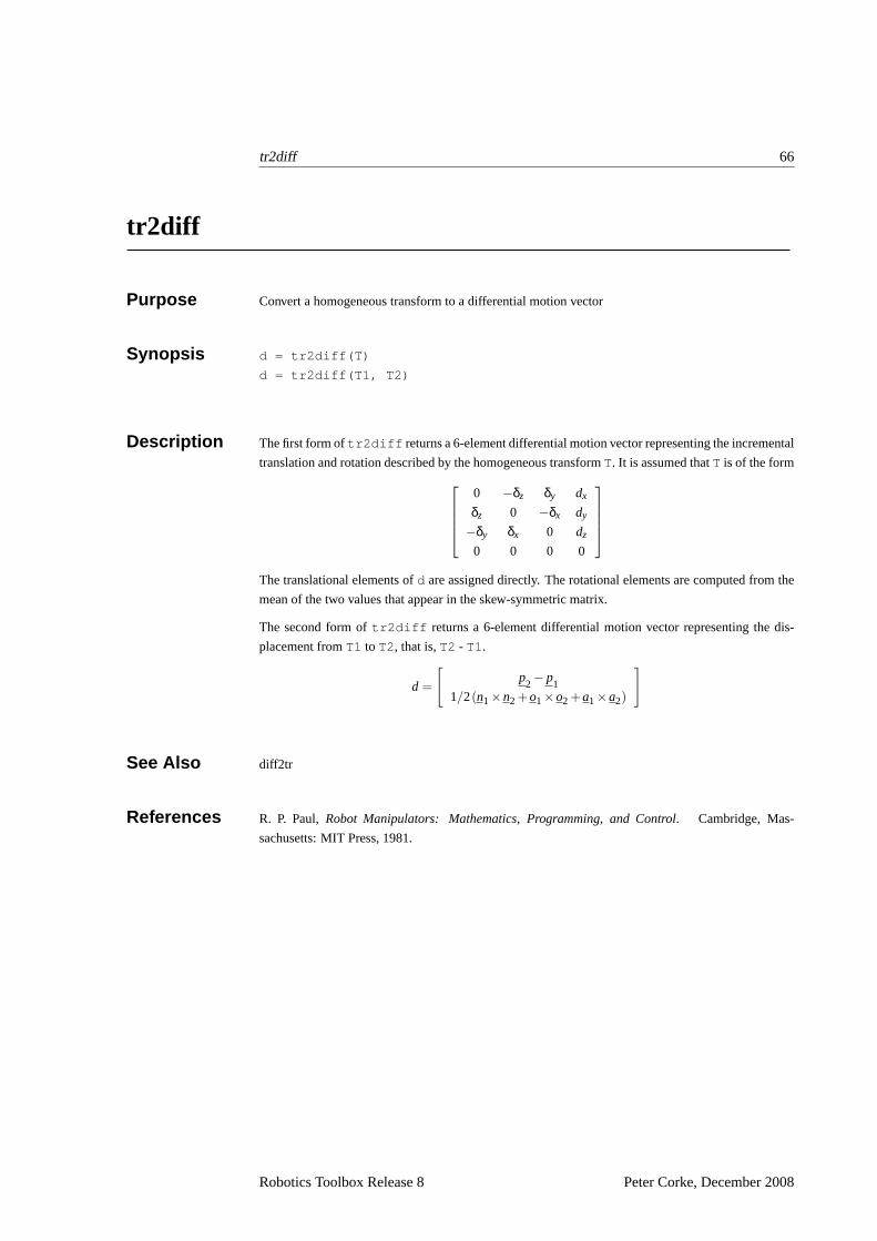
tr2diff 66
tr2diff
Purpose Convert a homogeneous transform to a differential motion vector
Synopsis d = tr2diff(T)
d = tr2diff(T1, T2)
Description The first form oftr2diff returns a 6-element differential motion vector representing the incremental
translation and rotation described by the homogeneous transformT. It is assumed thatT is of the form
0 −δz δy dx
δz 0 −δx dy
−δy δx 0 dz
0 0 0 0
The translational elements ofd are assigned directly. The rotational elements are computed from the
mean of the two values that appear in the skew-symmetric matrix.
The second form oftr2diff returns a 6-element differential motion vector representing the dis-
placement fromT1 to T2, that is,T2 - T1.
d =
[
p2− p
11/2(n1×n2 +o1×o2 +a1×a2)
]
See Also diff2tr
References R. P. Paul,Robot Manipulators: Mathematics, Programming, and Control. Cambridge, Mas-
sachusetts: MIT Press, 1981.
Robotics Toolbox Release 8 Peter Corke, December 2008
tr2eul 67
tr2eul
Purpose Convert a homogeneous transform or rotation matrix to Euler angles
Synopsis e = tr2eul(M)
Description Returns a vector of Euler angles [φ, θ, ψ], in radians, corresponding toM. Mis either a rotation matrix,
or the rotation part of the homogeneous transform is taken.
R = RZ(φ)RY (θ)RZ(ψ)
Cautionary Note that 12 different Euler angle sets or conventions exist. The convention used here is the common
one for robotics, but is not the one used for example in the aerospace community.
See Also eul2tr, tr2rpy
References R. P. Paul,Robot Manipulators: Mathematics, Programming, and Control. Cambridge, Mas-
sachusetts: MIT Press, 1981.
Robotics Toolbox Release 8 Peter Corke, December 2008
tr2jac 68
tr2jac
Purpose Compute a Jacobian to map differential motion between frames
Synopsis jac = tr2jac(T)
Description tr2jac returns a 6× 6 Jacobian matrix to map differential motions or velocities between frames
related by the homogeneous transformT.
If T represents a homogeneous transformation from frame A to frame B,ATB, then
Bx = BJAAx
whereBJA is given bytr2jac(T) .
See Also tr2diff, diff2tr
References R. P. Paul,Robot Manipulators: Mathematics, Programming, and Control. Cambridge, Mas-
sachusetts: MIT Press, 1981.
Robotics Toolbox Release 8 Peter Corke, December 2008
tr2rpy 69
tr2rpy
Purpose Convert a homogeneous transform or rotation matrix to roll/pitch/yaw angles
Synopsis e = tr2rpy(T)
Description Returns a vector of roll/pitch/yaw angles, [roll, pitch, yaw], in radians, corresponding toM. Mis either
a rotation matrix, or the rotation part of the homogeneous transform is taken.
R = RX (r)RY (p)RZ(y)
See Also rpy2tr, tr2eul
References R. P. Paul,Robot Manipulators: Mathematics, Programming, and Control. Cambridge, Mas-
sachusetts: MIT Press, 1981.
Robotics Toolbox Release 8 Peter Corke, December 2008
transl 70
transl
Purpose Translational transformation
Synopsis T = transl(x, y, z)
T = transl(v)
v = transl(T)
xyz = transl(TC)
Description The first two forms return a homogeneous transformation representing a translation expressed as three
scalarx , y andz , or a Cartesian vectorv .
The third form returns the translational part of a homogeneous transform as a 3-element column vector.
The fourth form returns a matrix whose columns are the X, Y and Z columns of the 4×4×m Cartesian
trajectory matrixTC.
See Also ctraj
Robotics Toolbox Release 8 Peter Corke, December 2008

trinterp 71
trinterp
Purpose Interpolate homogeneous transforms
Synopsis T = trinterp(T0, T1, r)
Description trinterp interpolates between the two homogeneous transformsT0 andT1 asr varies between 0
and 1 inclusively. This is generally used for computing straight line or ‘Cartesian’ motion. Rotational
interpolation is achieved using quaternion spherical linear interpolation.
Examples Interpolation of homogeneous transformations.
>> t1=rotx(.2)
t1 =
1.0000 0 0 0
0 0.9801 -0.1987 0
0 0.1987 0.9801 0
0 0 0 1.0000
>> t2=transl(1,4,5)*roty(0.3)
t2 =
0.9553 0 0.2955 1.0000
0 1.0000 0 4.0000
-0.2955 0 0.9553 5.0000
0 0 0 1.0000
>> trinterp(t1,t2,0) % should be t1
ans =
1.0000 0 0 0
0 0.9801 -0.1987 0
0 0.1987 0.9801 0
0 0 0 1.0000
>> trinterp(t1,t2,1) % should be t2
ans =
0.9553 0 0.2955 1.0000
0 1.0000 0 4.0000
-0.2955 0 0.9553 5.0000
0 0 0 1.0000
Robotics Toolbox Release 8 Peter Corke, December 2008

trinterp 72
>> trinterp(t1,t2,0.5) % ’half way’ in between
ans =
0.9887 0.0075 0.1494 0.5000
0.0075 0.9950 -0.0998 2.0000
-0.1494 0.0998 0.9837 2.5000
0 0 0 1.0000
>>
See Also ctraj, qinterp
References R. P. Paul,Robot Manipulators: Mathematics, Programming, and Control. Cambridge, Mas-
sachusetts: MIT Press, 1981.
Robotics Toolbox Release 8 Peter Corke, December 2008
trnorm 73
trnorm
Purpose Normalize a homogeneous transformation
Synopsis TN = trnorm(T)
Description Returns a normalized copy of the homogeneous transformationT. Finite word length arithmetic can
lead to homogeneous transformations in which the rotational submatrix is not orthogonal, that is,
det(R) 6= −1.
Algorithm Normalization is performed by orthogonalizing the rotation submatrixn = o×a, o = a×n.
See Also oa2tr
References J. Funda, “Quaternions and homogeneous transforms in robotics,” Master’s thesis, University of Penn-
sylvania, Apr. 1988.
Robotics Toolbox Release 8 Peter Corke, December 2008

trplot 74
trplot
Purpose Plot a homogeneous transform
Synopsis trplot(T)
Description Displays a 3D plot which shows how the standard axes are transformed by the transformationT.
Examples Display the coordinate frame represented by a homogeneous transform.
>> tr = trotx(.2)*troty(.3)*transl(1,2,3)
ans =
0.9553 0 0.2955 1.8419
0.0587 0.9801 -0.1898 1.4495
-0.2896 0.1987 0.9363 2.9166
0 0 0 1.0000
>> trplot(tr)
0
1
2
3
4 01
23
4
0
0.5
1
1.5
2
2.5
3
3.5
4
Y
Y
X
Z
X
Z
See Also @quaternion/plot
Robotics Toolbox Release 8 Peter Corke, December 2008
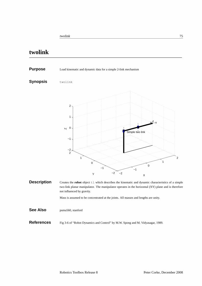
twolink 75
twolink
Purpose Load kinematic and dynamic data for a simple 2-link mechanism
Synopsis twolink
−2−1
01
2
−2
−1
0
1
2−2
−1
0
1
2
XY
Z
Simple two link
xy z
Description Creates therobot object tl which describes the kinematic and dynamic characteristics of a simple
two-link planar manipulator. The manipulator operates in the horizontal (XY) plane and is therefore
not influenced by gravity.
Mass is assumed to be concentrated at the joints. All masses and lengths are unity.
See Also puma560, stanford
References Fig 3-6 of “Robot Dynamics and Control” by M.W. Spong and M. Vidyasagar, 1989.
Robotics Toolbox Release 8 Peter Corke, December 2008

unit 76
unit
Purpose Unitize a vector
Synopsis vn = unit(v)
Description unit returns a unit vector aligned withv .
Algorithmvn =
v||v||
Robotics Toolbox Release 8 Peter Corke, December 2008
Related Documents


