Robot Motion Planning Computational Geometry Lecture by Stephen A. Ehmann.

Robot Motion PlanningRobot Motion Planning

Computational Geometry Lecture

by

Stephen A. Ehmann

Motivation

• Want to design autonomous robots– performs actions without being told how

• Robot must be able to plan its motion– has a map of the environment

• We will focus on collision-free motion

• There is a tradeoff between having an easy/fast solution and being conservative

Defining the General Problem

• Environment may vary over time

• Other robots may exist in the environment– coordinated motion problems

• There may be constraints on the motion– Ex. Minimum turning radius– Ex. Maximum displacement of a prismatic joint

Defining the General Problem

• There may be a cost function to minimize or maximize– time, distance, energy, safety

• The robot can have many degrees of freedom (DOF)– translation, rotation, joints (revolute, prismatic)

Lots of DOF Possible!

Defining a Simpler Problem

• Environment does not vary over time

• Single robot in the environment

• No constraints on the allowed motion

• No cost function

• Polygonal obstacles and robot

• Allowed to touch obstacles– can always enlarge the robot for safety margin

Example Problem

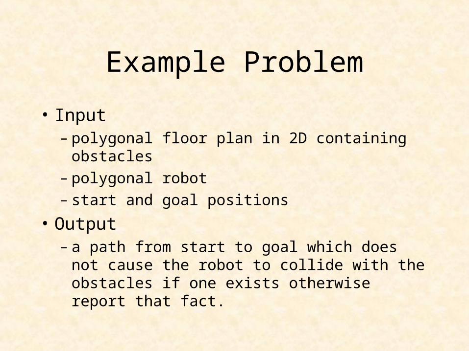
• Input– polygonal floor plan in 2D containing obstacles– polygonal robot– start and goal positions

• Output– a path from start to goal which does not cause

the robot to collide with the obstacles if one exists otherwise report that fact.

Example Problem

Outline

• Motivation• Defining the Problem• Work Space and

Configuration Space• Minkowski Sums• Point Robot Solution

• Rotations• Three and Higher

Dimensions• Conclusions• References

Work Spaceand

Configuration Space

• Work Space (WS) is the space of the original problem (the real world)

• Configuration Space (CS) is the parameter space of the problem (more abstract)

Work Spaceand

Configuration Space

Robot Reference Point• A robot has a reference point which

uniquely determines placement according to the allowed degrees of freedom

Reference Point in CS

• A point in the CS corresponds to a placement of a robot in WS

• This point is exactly the reference point of the robot in WS for our example

Free/Forbidden Space

• Free configuration space (free space) is the set of all points in CS such that the corresponding robot placements in WS do not intersect any of the obstacles

• Forbidden configuration space (forbidden space) is the set of all point in CS such that the corresponding robot placements in WS intersect with at least one of the obstacles

Paths

• A path is a curve through CS– moves continuously from one set of parameter

values to another– is the curve traveled by the point representing

the placement of the robot in WS

• A collision-free path is a curve wholly contained within the free space

Mapping from WS to CSfor our Example

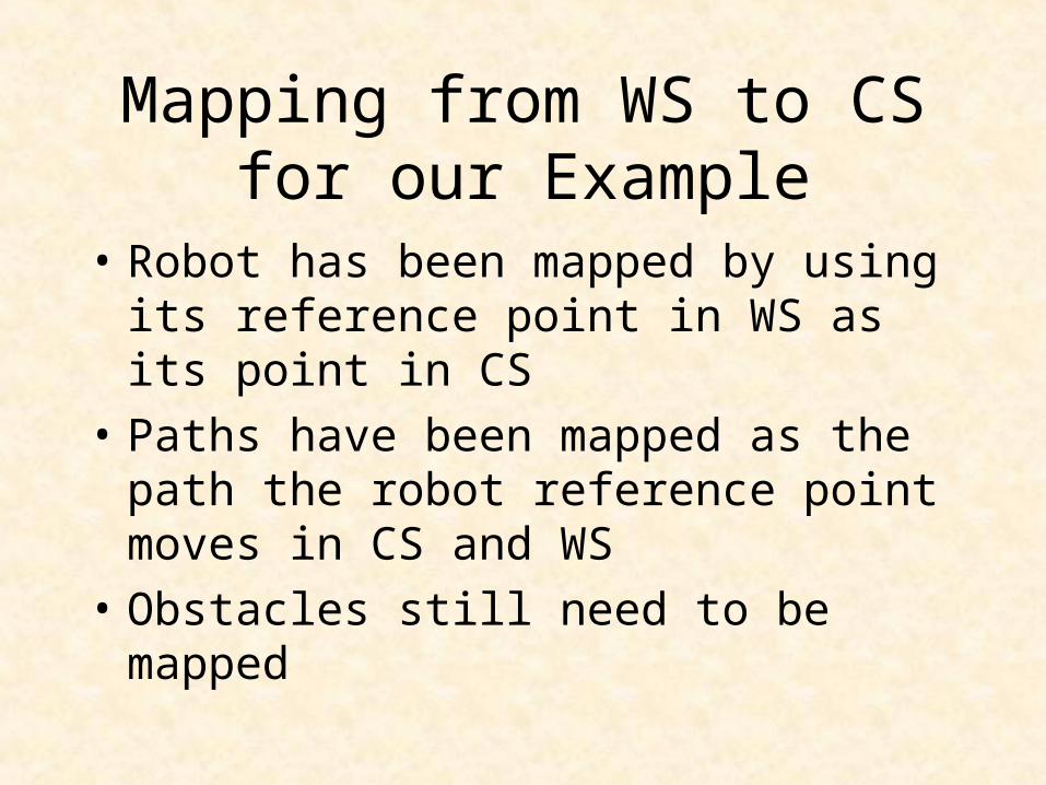
• Robot has been mapped by using its reference point in WS as its point in CS

• Paths have been mapped as the path the robot reference point moves in CS and WS

• Obstacles still need to be mapped

Mapping Obstacles

• Intuitively it can be seen that we need to enlarge the obstacles in some manner when mapping them from WS to CS

• The union of the maps of the obstacles will become the forbidden space -- the rest of CS will be the free space

Mapping Obstacles

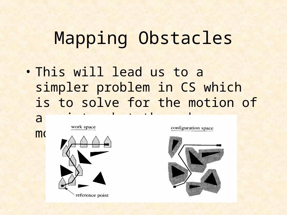
• This will lead us to a simpler problem in CS which is to solve for the motion of a point robot through a modified obstacle field

Mapping Obstacles

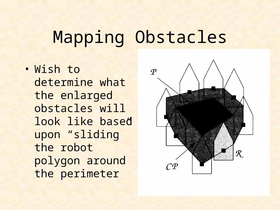
• Wish to determine what the enlarged obstacles will look like based upon “sliding” the robot polygon around the perimeter

Minkowski Sums

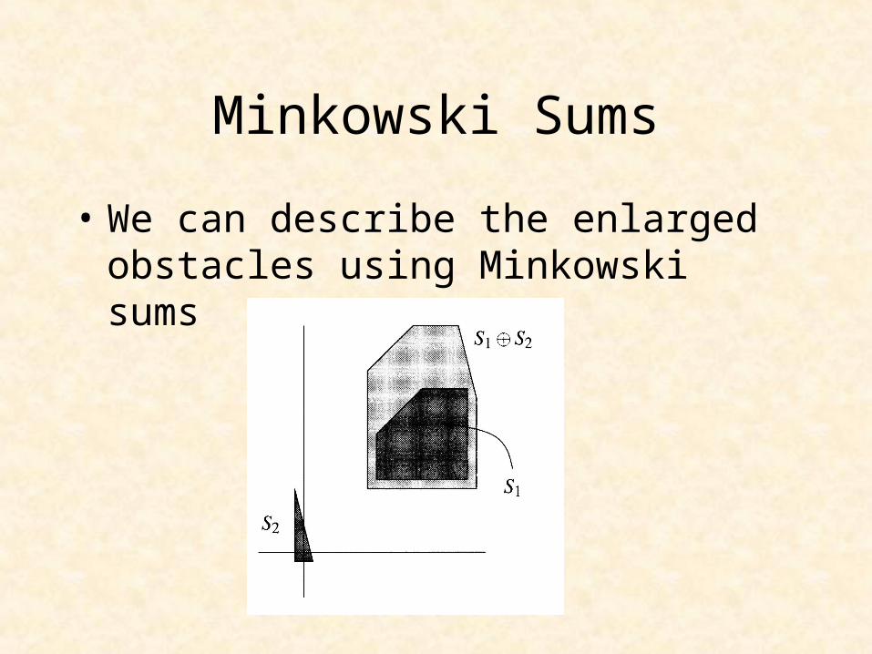
• We can describe the enlarged obstacles using Minkowski sums

Minkowski Sums

• S1 S2 = {p+q : p S1, q S2} where– p = (px, py)

– q = (qx, qy)

– p+q = (px+qx, py+qy)

• The mapping of a polygonal obstacle P to CS is P (-R(0,0)) where R(0,0) is the robot with its reference point at (0,0)

Proof of the Mapping

• Suppose robot R(x,y) intersects obstacle P at q = (qx, qy)

• q R(x,y) ==> (qx - x, qy - y) R(0,0) | ==> (-qx + x, -qy + y) (-R(0,0))

• q P ==> (qx, qy ) P | ==> (qx+ (-qx + x), qy + (-qy + y)) | P (-R(0,0)) | ==> (x,y) P (-R(0,0))

Minkowski Sums

• Let P and R be two convex polygons with n and m edges respectively. Then P R is a convex polygon with at most m+n edges.

• Intuitively, each edge on the original polygons generates an edge on P R

Minkowski Sums

Computing Minkowski Sums

• Want to compute the Minkowski sum of

two convex polygons

• Can add each pair of vertices (one from each polygon) and then compute the convex hull of the resulting point set O(mn log mn)

• We can however make the algorithm run in linear time O(m+n)!

Computing Minkowski Sums

• Observe that an extreme point on P R in a direction d is the sum of the extreme points in direction d on P and R

• This means that we can use a gift wrapping method to compute the desired convex hull without considering points not on the convex hull boundary. It is like the merge step from merge sort.

Computing Minkowski Sums

• Each polygon is has its vertices sorted in counter-clockwise order and the first vertex has the smallest y coordinate

• Add edges with the smallest angle first

Computing Minkowski SumsMINKOWSKI-SUM(P,R)

1. i := 1; j := 1

2. vn+1 := v1; wm+1 := w1

3. repeat

4. Add v i + w j as a vertex to PR

5. if angle( vi vi+1 ) < angle( wj wj+1 ) then

6. i := i + 1

7. else if angle( vi vi+1 ) > angle( wj wj+1 ) then

8. j := j + 1

9. else

10. i := i + 1; j := j + 1

11. until i = n+1 and j = m+1

Unions of Minkowski Sums

• The following property holds:– S1 (S2 S3) = (S1S2) (S1S3)

• To deal with non-convex polygons, we can first triangulate them and then take the union of all Minkowski sums generated by all the pairs of triangles

P R = (i=1..n-2, j=1..m-2) ti uj

where the ti are the triangles from P and the uj are from R

Complexity of Minkowski Sums

• O(m+n) if both polygons are convex

• O(mn) if one of the polygons is convex and the other is not

• O(m2n2) if both polygons are non-convex

Minkowski Sum Demo

Outline

• Motivation• Defining the Problem• Work Space and

Configuration Space• Minkowski Sums• Point Robot Solution

• Rotations• Three and Higher

Dimensions• Conclusions• References

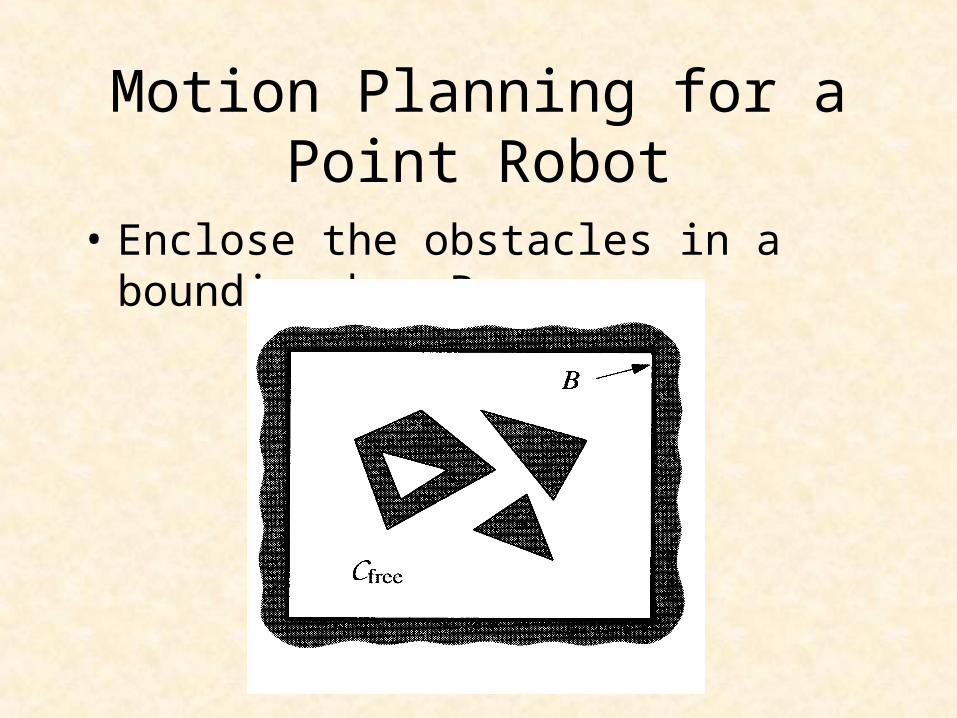
Motion Planning for aPoint Robot

• Enclose the obstacles in a bounding box B

Computing the Free Space

• Want to compute a representation of the free space within which we can find a free path

COMPUTE-FREE-SPACE

1. Let E be the set of edges of the obstacles

2. Compute the trapezoidal map T(E) (from Ch. 6)

3. Remove the trapezoids that lie inside the obstacles

Computing the Free Space• Recall that the trapezoidal map is constructed

in O(n log n) expected time where n is the number of edges in the set of the obstacles

• The step of removing the unwanted trapezoids takes O(n) time since we must simply check for each trapezoid whether the top of it is an edge that bounds an obstacle from above or from below

Computing Paths• Need a road map through the trapezoids

• Create a graph with a vertex– in the middle of each vertical extension– in the middle of each trapezoid

• Connect vertices in the center of a trapezoid with the vertices on the edges of the same trapezoid

• Can create the road map in O(n) time

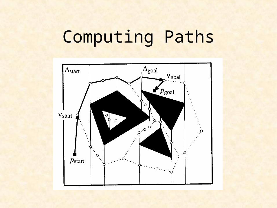
Computing Paths

Computing Paths

• Use the point location structure that is built along with the trapezoidal map to lookup the start and goal trapezoids

• If the start and the goal points are in the same trapezoid, the robot can simply move in a straight line from start to goal

Computing Paths

• Connect the start and goal points to the vertices in the center of their respective trapezoids

• Use breadth-first search to compute the path connecting the start and goal trapezoid centers if one exists

Point Robot Solution

• Free space can be computed in O(n log n) time

• A collision free path can then be computed in O(n) time

• The complexity of the free space representation is O(n)

• The road map also has a complexity of O(n)

Polygonal Robot Solution

• For a convex robot R, the obstacles can be preprocessed in O(n log2 n) expected time

• A path can then be computed in O(n) time if it exists

Outline

• Motivation• Defining the Problem• Work Space and

Configuration Space• Minkowski Sums• Point Robot Solution

• Rotations• Three and Higher

Dimensions• Conclusions• References

Rotations

• If a robot is allowed rotation in addition to translation in 2D then it has 3 DOF

• The configuration space is 3D: (x,y,φ) where φ is in the range [0:360)

Mapping to CS

• The obstacles map to “twisted pillars” in CS

• They are no longer polygonal but are composed of curved faces and edges

Computing Free Space

• Exact cell decomposition is really hard

• Compute z: a finite number of slices for discrete angular values

• Each slice will be the representation of the free space for a purely translational problem

• Robot will either move within a slice (translating) or between slices (rotating)

Computing the Road Map

• Each slice has a road map like before

• But how do we move between slices?

Moving Between Slices

• To find graph edges between two slices:

1. compute the overlay of the trapezoidal maps of the two slices to get all pairs of trapezoids that

intersect (one trapezoid from each slice)2. for each pair3. find a point (x,y) in their intersection and make one new vertex in each slice at this (x,y) 4. connect the two new vertices5. connect the each of the two new vertices to the

vertex at the center of their respective trapezoids

Slice Problems (Aliasing)

• Start and/or goal position may be in the free space whereas the start/goal position in the nearest slice may not

• May have an undetected collision when moving between slices

• Increasing the number of slices reduces problems but does not solve them

Dealing with the Problems

• Enlarge the robot by sweeping out some additional area (180o/z) in each direction

• Introduces yet another way to incorrectly determine that there is no path

Three Dimensional Translation

• Have k obstacles, each bounded by n edges

• Have 3 DOF

• Compute 3D Minkowski sums and then compute the 3D equivalent of a trap. map

• Compute the graph and then search it to find the solution

• The space has complexity O(nk log2k)

• Expected construction time is O(nk log3k )

Three Dimensions with the Addition of Rotations

• Have k obstacles, each bounded by n edges

• Have 6 DOF

• Do something similar to the slice method

• Slices now become cells in the 3D space representing rotations– each cell has the purely translational solution for

the set of orientations that it represents– move to 6 adjacent cells (3 different rotations)

Three Dimensions with the Addition of Rotations

• Moving from cell to cell represents rotating about one of the three axes

• Have the same problems we had with slices– Start and/or goal position may be in the free space

whereas the start/goal position in the nearest cell may not

– May have an undetected collision when moving between cells

– Increasing the number of cells reduces problems but does not solve them

A Word about Higher Dimensions

• When we have d DOF we have a d-dimensional CS

• Adding constraints to the motion restricts the range of some of the dimensions of CS– May need additional geometric primitives to

represent these constraints

Higher Dimensions

• J. Canny has proposed a very general and “complicated” road map method to solve any motion planning problem exactly– O(nd log n) time where d is the dimension of

the configuration space (DOF)– disadvantage is that the robot moves in contact

with an obstacle most of the time which is not usually desirable

Approximate Cell Decomposition

Approximate Cell Decomposition

• Use a 2m-tree to represent free CS having empty, full, and mixed types of cells

+ Easier, faster than exact methods

+ Minimum size of cells controls the amount of free space surrounding a generated path• Measure of safety cost

– Conservative• May miss solutions

Potential Field Methods

Potential Field Methods

• At each step move an increment in the direction that minimizes the energy

+ Good heuristic for high DOF

– Can get trapped in local minima• use some probabilistic motion to escape

– Oscillations can also occur

Probabilistic Methods

• Throw darts into free space to generate graph vertices

• Search the graph to find a path

+ Easy

– May generate “bad” paths

– May miss paths

Conclusions

• Have concentrated on exact motion planning: there are other heuristics– approximate cell decompositions (2m-tree)– potential field methods (minimize energy)– probabilistic road map (throw darts)

• Have not worried about:– lowest cost path, motion constraints, changing

environment, multiple robots

References

• “Computational Geometry -- Algorithms and Applications” by de Berg, van Kreveld, Overmars, and Schwarzkopf - 1997

• “Robot Motion Planning” by Latombe 1991

• “On translational motion planning in 3-space” by Aronov and Sharir - Proc. 10th Annu. ACM Sympos. Comput. Geom. 1994