HAL Id: tel-01555492 https://tel.archives-ouvertes.fr/tel-01555492 Submitted on 4 Jul 2017 HAL is a multi-disciplinary open access archive for the deposit and dissemination of sci- entific research documents, whether they are pub- lished or not. The documents may come from teaching and research institutions in France or abroad, or from public or private research centers. L’archive ouverte pluridisciplinaire HAL, est destinée au dépôt et à la diffusion de documents scientifiques de niveau recherche, publiés ou non, émanant des établissements d’enseignement et de recherche français ou étrangers, des laboratoires publics ou privés. Robot-assisted bone cement injection Nicole Lepoutre To cite this version: Nicole Lepoutre. Robot-assisted bone cement injection. Surgery. Université de Strasbourg, 2016. English. NNT : 2016STRAD049. tel-01555492

Welcome message from author
This document is posted to help you gain knowledge. Please leave a comment to let me know what you think about it! Share it to your friends and learn new things together.
Transcript
HAL Id: tel-01555492https://tel.archives-ouvertes.fr/tel-01555492
Submitted on 4 Jul 2017
HAL is a multi-disciplinary open accessarchive for the deposit and dissemination of sci-entific research documents, whether they are pub-lished or not. The documents may come fromteaching and research institutions in France orabroad, or from public or private research centers.
L’archive ouverte pluridisciplinaire HAL, estdestinée au dépôt et à la diffusion de documentsscientifiques de niveau recherche, publiés ou non,émanant des établissements d’enseignement et derecherche français ou étrangers, des laboratoirespublics ou privés.
Robot-assisted bone cement injectionNicole Lepoutre
To cite this version:Nicole Lepoutre. Robot-assisted bone cement injection. Surgery. Université de Strasbourg, 2016.English. �NNT : 2016STRAD049�. �tel-01555492�


Für Markus
Aan mijn ouders
À Suz et Flo

Acknowledgements
First of all, I would like to thank the thesis committee members and especially the external examiners Pr. Philippe
Poignet, Pr. Alexander Lion and Pr. Philippe Cinquin for having accepted to read and evaluate my work and for
all the constructive comments and questions during the defense.
Je remercie le Ministère de l’Enseignement supérieur et de la Recherche pour m’avoir attribué une allocation de
recherche mais aussi la SATT Conectus Alsace pour avoir financé le projet S-Tronic, et enfin l’INSA de Strasbourg
pour le poste d’ATER.
J’adresse ensuite mes remerciements à Bernard, mon directeur de thèse, pour m’avoir proposé ce sujet et pour
m’avoir fait confiance tout au long de ce travail. En plus d’être un porteur de projet hors norme, ses conseils, ses
astuces et son expertise ont toujours été des aides précieuses.
J’ai aussi pu compter sur deux encadrantes exceptionnelles: Laurence et Iulia. Dans leur domaine respectif,
elles ont su m’apprendre de nombreuses choses indispensables à l’avancement de ma thèse avec beaucoup
d’enthousiasme et toujours dans la bonne humeur. Un grand merci supplémentaire à Laurence pour les
centaines d’heures de manips qui n’ont jamais été ennuyantes!
Je tiens ensuite à remercier François et Laurent, nos deux ingénieurs du projet. Que ce soit en mécanique,
électronique ou informatique, ils ont toujours pris le temps de m’éclairer sur ces aspects en répondant à
nombreuses de mes questions aussi bêtes qu’elles soient.
Ce projet inclut la collaboration avec l’IEF. Dans ce cadre, je tiens à remercier Élie et Émile pour nos nombreux
échanges constructifs.
Je tiens aussi à remercier Afshin Gangi et Julien Garnon de m’avoir ouvert les portes du service de radiologie
interventionnelle du NHC pour je puisse comprendre en détail la pratique de la vertébroplastie en assistant à
plusieurs interventions mais aussi pour leurs retours sur le dispositif.
Une très grande reconnaissance pour la société Heraeus mais plus particulièrement pour Mme Lestang qui
nous a donné un nombre incalculable de kits de ciment sans lesquels les résultats présentés dans la suite du
manuscrit n’auraient pas pu être obtenus.
Avant de démarrer cette thèse, je n’aurais pas pu imaginer à quel point le cadre de travail serait agréable au
sein de l’équipe AVR. Ainsi, je souhaite remercier l’ensemble des personnes de notre équipe pour l’accueil et
l’ambiance de travail. Tout au long de ces années, cet épanouissement a été amplifié grâce aux autres doctorants,
aux stagiaires, ... formant un superbe groupe d’amis. Merci donc à Nadège, Quentin et Paolo (deux collègues de
bureau parfaits!), Émeric, Gauthier, Cédric, Benoît, Arnaud, François, Mathilde (c’est tout comme!) et Laure.
v
Acknowledgements
Pour se changer les idées, quoi de mieux que de se retrouver autour de la balle orange. Je remercie donc toute
l’équipe de l’élec et surtout les anciennes comme Élise, Pauline et Claire.
De grootste dank gaat naar mijn ouders en mijn twee kleine zusjes. Ze zijn er altijd geweest om mij te steunen en
te begeleiden in mijn keuzes. Jullie zijn altijd heel trots op mij geweest en ik hope dat dat nog lang zal duren.
Ich möchte meine Danksagung mit dem Besten beschließen, das mir während meiner PhD-Phase passiert ist: Ich
habe Markus kennen gelernt. Während dieser beiden letzten Jahre wusste er immer, wie er mich unterstützen,
ermutigen, mir Rat geben und mich in schwierigen Zeiten aufmuntern kann. Und darüber hinaus danke ich
ihm für all seine Liebe und die wundervollen Augenblicke, die wir miteinander geteilt haben.
vi
Abstract - Résumé
Abstract
Percutaneous vertebroplasty is a minimally invasive intervention that involves injecting bone cement, under
fluoroscopic guidance, into the vertebral body. It consolidates the fractured vertebra and reduces pain. However,
some inconveniences must be considered. The major difficulties are related to the cement that is injected during
its curing phase. It is very liquid at the beginning of the injection, which introduces a high risk of leakage outside
the vertebra and, thus, potential dramatic complications. During the injection, the reaction progresses and
the cement hardens suddenly, leaving a short working phase. Finally, the operator is permanently exposed to
harmful X-rays.
This work aims to provide a new teleoperated injection device with haptic feedback that allows a fine supervision
of the cement injection by including a viscosity control system. This device will allow the radioprotection of the
medical staff, a reduction of the leakage risks and an extended injection phase.
Key words: Rheology, Modeling, Control, Medical robotics.
Résumé
La vertébroplastie percutanée est une intervention non chirurgicale et peu invasive qui consiste à injecter, sous
contrôle radioscopique, un ciment orthopédique dans le corps vertébral. Malgré son efficacité, celle-ci présente
quelques inconvénients non négligeables. Le premier est dû au ciment orthopédique qui est injecté pendant
sa polymérisation. Au début, sa faible viscosité augmente le risque de fuite hors de la vertèbre traitée, ce qui
peut provoquer de lourdes complications. Ensuite, la variation rapide de viscosité limite la durée. Le second
désagrément concerne le contrôle par fluoroscopie à rayons X qui expose le praticien de manière prolongée.
Ainsi, l’enjeu de ce projet est de proposer aux radiologues un nouveau système d’injection à distance avec
retour d’effort sur lequel la viscosité du ciment est régulée pendant l’injection. Le développement de ces aspects
permettra la radioprotection des praticiens, une réduction des risques de fuite et une durée d’injection allongée.
Mots-clés : Rhéologie, Modélisation, Automatique, Robotique médicale.

Contents
Acknowledgements v
Abstract - Résumé vii
List of figures xvi
List of tables xvii
Nomenclature xix
1 Problem statement 11.1 Spine health . . . . . . . . . . . . . . . . . . . . . . . . . . . . . . . . . . . . . . . . . . . . . . . . . . . 2
1.1.1 General spine anatomy . . . . . . . . . . . . . . . . . . . . . . . . . . . . . . . . . . . . . . . . 2
1.1.2 Vertebral compression fractures . . . . . . . . . . . . . . . . . . . . . . . . . . . . . . . . . . . 5
1.1.3 Proposed treatments . . . . . . . . . . . . . . . . . . . . . . . . . . . . . . . . . . . . . . . . . . 6
1.2 Percutaneous vertebroplasty . . . . . . . . . . . . . . . . . . . . . . . . . . . . . . . . . . . . . . . . . 8
1.2.1 History and current state . . . . . . . . . . . . . . . . . . . . . . . . . . . . . . . . . . . . . . . 8
1.2.2 Acrylic bone cements . . . . . . . . . . . . . . . . . . . . . . . . . . . . . . . . . . . . . . . . . 9
1.2.3 Procedure . . . . . . . . . . . . . . . . . . . . . . . . . . . . . . . . . . . . . . . . . . . . . . . . 13
1.2.4 Benefits . . . . . . . . . . . . . . . . . . . . . . . . . . . . . . . . . . . . . . . . . . . . . . . . . . 16
1.2.5 Complications and drawbacks . . . . . . . . . . . . . . . . . . . . . . . . . . . . . . . . . . . . 16
1.3 Available injection tools . . . . . . . . . . . . . . . . . . . . . . . . . . . . . . . . . . . . . . . . . . . . 17
1.3.1 Manual systems . . . . . . . . . . . . . . . . . . . . . . . . . . . . . . . . . . . . . . . . . . . . . 17
1.3.2 Mechatronic systems . . . . . . . . . . . . . . . . . . . . . . . . . . . . . . . . . . . . . . . . . . 19
1.3.3 S-Tronic project . . . . . . . . . . . . . . . . . . . . . . . . . . . . . . . . . . . . . . . . . . . . . 21
1.4 Thesis contributions and organization . . . . . . . . . . . . . . . . . . . . . . . . . . . . . . . . . . . 22
1.4.1 Thesis contributions . . . . . . . . . . . . . . . . . . . . . . . . . . . . . . . . . . . . . . . . . . 22
1.4.2 Thesis organization . . . . . . . . . . . . . . . . . . . . . . . . . . . . . . . . . . . . . . . . . . . 22
2 Rheology of bone cement 232.1 Aspects of rheology . . . . . . . . . . . . . . . . . . . . . . . . . . . . . . . . . . . . . . . . . . . . . . . 24
2.1.1 Definitions . . . . . . . . . . . . . . . . . . . . . . . . . . . . . . . . . . . . . . . . . . . . . . . . 24
2.1.2 Rheological behaviors . . . . . . . . . . . . . . . . . . . . . . . . . . . . . . . . . . . . . . . . . 25
2.1.3 Rheometers . . . . . . . . . . . . . . . . . . . . . . . . . . . . . . . . . . . . . . . . . . . . . . . 26
2.2 Acrylic bone cement . . . . . . . . . . . . . . . . . . . . . . . . . . . . . . . . . . . . . . . . . . . . . . 29
2.2.1 Chemical aspect . . . . . . . . . . . . . . . . . . . . . . . . . . . . . . . . . . . . . . . . . . . . 29
2.2.2 Bone cement rheological properties . . . . . . . . . . . . . . . . . . . . . . . . . . . . . . . . . 30
ix
Contents
2.2.3 Viscosity modeling . . . . . . . . . . . . . . . . . . . . . . . . . . . . . . . . . . . . . . . . . . . 31
2.3 Rheological study . . . . . . . . . . . . . . . . . . . . . . . . . . . . . . . . . . . . . . . . . . . . . . . . 34
2.3.1 Viscosity measurement . . . . . . . . . . . . . . . . . . . . . . . . . . . . . . . . . . . . . . . . 34
2.3.2 Experiments . . . . . . . . . . . . . . . . . . . . . . . . . . . . . . . . . . . . . . . . . . . . . . . 36
2.3.3 Analysis . . . . . . . . . . . . . . . . . . . . . . . . . . . . . . . . . . . . . . . . . . . . . . . . . 38
3 Modeling and identification of bone cement viscosity 413.1 Modified Power law . . . . . . . . . . . . . . . . . . . . . . . . . . . . . . . . . . . . . . . . . . . . . . . 42
3.1.1 Motivation and contributions . . . . . . . . . . . . . . . . . . . . . . . . . . . . . . . . . . . . . 42
3.1.2 Identification of the functions n and K . . . . . . . . . . . . . . . . . . . . . . . . . . . . . . . 42
3.1.3 Temperature influence . . . . . . . . . . . . . . . . . . . . . . . . . . . . . . . . . . . . . . . . . 45
3.1.4 Validation . . . . . . . . . . . . . . . . . . . . . . . . . . . . . . . . . . . . . . . . . . . . . . . . 49
3.2 Differential equation . . . . . . . . . . . . . . . . . . . . . . . . . . . . . . . . . . . . . . . . . . . . . . 50
3.2.1 Motivation and contributions . . . . . . . . . . . . . . . . . . . . . . . . . . . . . . . . . . . . . 50
3.2.2 Choice of the model . . . . . . . . . . . . . . . . . . . . . . . . . . . . . . . . . . . . . . . . . . 50
3.2.3 Phase space identification . . . . . . . . . . . . . . . . . . . . . . . . . . . . . . . . . . . . . . . 52
3.2.4 Validation . . . . . . . . . . . . . . . . . . . . . . . . . . . . . . . . . . . . . . . . . . . . . . . . 57
4 S-Tronic robot for teleoperated bone cement injection 594.1 Robotic injection device . . . . . . . . . . . . . . . . . . . . . . . . . . . . . . . . . . . . . . . . . . . . 60
4.1.1 Design and instrumentation . . . . . . . . . . . . . . . . . . . . . . . . . . . . . . . . . . . . . 60
4.1.2 Disposable items . . . . . . . . . . . . . . . . . . . . . . . . . . . . . . . . . . . . . . . . . . . . 62
4.1.3 Passive cooling . . . . . . . . . . . . . . . . . . . . . . . . . . . . . . . . . . . . . . . . . . . . . 64
4.1.4 Control of the injection device . . . . . . . . . . . . . . . . . . . . . . . . . . . . . . . . . . . . 66
4.2 Design of a temperature control system . . . . . . . . . . . . . . . . . . . . . . . . . . . . . . . . . . . 66
4.2.1 Positioning of the temperature exchanger . . . . . . . . . . . . . . . . . . . . . . . . . . . . . 66
4.2.2 Dimensioning of the temperature exchanger . . . . . . . . . . . . . . . . . . . . . . . . . . . . 68
4.2.3 Technology of the temperature exchanger . . . . . . . . . . . . . . . . . . . . . . . . . . . . . 71
4.2.4 Validation by numerical simulations . . . . . . . . . . . . . . . . . . . . . . . . . . . . . . . . . 72
4.3 Teleoperated cement injection . . . . . . . . . . . . . . . . . . . . . . . . . . . . . . . . . . . . . . . . 74
4.3.1 Master device . . . . . . . . . . . . . . . . . . . . . . . . . . . . . . . . . . . . . . . . . . . . . . 74
4.3.2 Teleoperation background . . . . . . . . . . . . . . . . . . . . . . . . . . . . . . . . . . . . . . 75
4.3.3 Rate control strategy . . . . . . . . . . . . . . . . . . . . . . . . . . . . . . . . . . . . . . . . . . 77
4.4 Experiments . . . . . . . . . . . . . . . . . . . . . . . . . . . . . . . . . . . . . . . . . . . . . . . . . . . 79
4.4.1 Experimental set-up . . . . . . . . . . . . . . . . . . . . . . . . . . . . . . . . . . . . . . . . . . 79
4.4.2 Experimental results . . . . . . . . . . . . . . . . . . . . . . . . . . . . . . . . . . . . . . . . . . 79
5 Online estimation and control of bone cement viscosity 835.1 Temperature control . . . . . . . . . . . . . . . . . . . . . . . . . . . . . . . . . . . . . . . . . . . . . . 84
5.1.1 Modeling and identification of the thermal block . . . . . . . . . . . . . . . . . . . . . . . . . 85
5.1.2 Temperature closed-loop control . . . . . . . . . . . . . . . . . . . . . . . . . . . . . . . . . . 90
5.1.3 Effect of temperature changes on the cement mechanical properties . . . . . . . . . . . . . 97
5.2 Viscosity estimation and control . . . . . . . . . . . . . . . . . . . . . . . . . . . . . . . . . . . . . . . 98
5.2.1 Online estimation of the bone cement viscosity . . . . . . . . . . . . . . . . . . . . . . . . . . 98
5.2.2 Viscosity control . . . . . . . . . . . . . . . . . . . . . . . . . . . . . . . . . . . . . . . . . . . . 103
6 Conclusions and perspectives 1076.1 Conclusions . . . . . . . . . . . . . . . . . . . . . . . . . . . . . . . . . . . . . . . . . . . . . . . . . . . 107
6.2 Perspectives . . . . . . . . . . . . . . . . . . . . . . . . . . . . . . . . . . . . . . . . . . . . . . . . . . . 108
6.2.1 Transfer perspectives . . . . . . . . . . . . . . . . . . . . . . . . . . . . . . . . . . . . . . . . . . 108
6.2.2 Evolution of the temperature control module . . . . . . . . . . . . . . . . . . . . . . . . . . . 109
x
Contents
6.2.3 Intravertebral pressure . . . . . . . . . . . . . . . . . . . . . . . . . . . . . . . . . . . . . . . . . 110
6.2.4 Dielectric measurements . . . . . . . . . . . . . . . . . . . . . . . . . . . . . . . . . . . . . . . 111
A Hagen-Poiseuille equation 113
B Transient convective heat transfer 117
C Numerical resolution of the heat equation 119
D Résumé en français 123D.1 Contexte médical . . . . . . . . . . . . . . . . . . . . . . . . . . . . . . . . . . . . . . . . . . . . . . . . 123
D.2 Rhéologie des ciments orthopédiques . . . . . . . . . . . . . . . . . . . . . . . . . . . . . . . . . . . . 124
D.3 Modélisation et identification de la viscosité du ciment orthopédique . . . . . . . . . . . . . . . . . 127
D.3.1 Loi puissance modifiée . . . . . . . . . . . . . . . . . . . . . . . . . . . . . . . . . . . . . . . . 127
D.3.2 Equation différentielle . . . . . . . . . . . . . . . . . . . . . . . . . . . . . . . . . . . . . . . . . 129
D.4 Robot S-Tronic pour une injection de ciment télé-opérée . . . . . . . . . . . . . . . . . . . . . . . . 130
D.4.1 Dispositif esclave . . . . . . . . . . . . . . . . . . . . . . . . . . . . . . . . . . . . . . . . . . . . 130
D.4.2 Dispositif maître . . . . . . . . . . . . . . . . . . . . . . . . . . . . . . . . . . . . . . . . . . . . 131
D.4.3 Bloc de régulation thermique . . . . . . . . . . . . . . . . . . . . . . . . . . . . . . . . . . . . . 131
D.5 Estimation en ligne et contrôle de la viscosité du ciment . . . . . . . . . . . . . . . . . . . . . . . . . 132
D.5.1 Contrôle de la température . . . . . . . . . . . . . . . . . . . . . . . . . . . . . . . . . . . . . . 133
D.5.2 Contrôle de la viscosité . . . . . . . . . . . . . . . . . . . . . . . . . . . . . . . . . . . . . . . . 133
D.6 Conclusions . . . . . . . . . . . . . . . . . . . . . . . . . . . . . . . . . . . . . . . . . . . . . . . . . . . 134
References 135
List of publications 145
xi

List of figures
1.1 Left lateral view of the spinal column anatomy, adapted from [AnatomyExpert 2016]. . . . . . . . . 3
1.2 Superior view of a typical cervical, thoracic and lumbar vertebra, adapted from [Strang 2006]. . . 4
1.3 Comparison between normal bone density and reduced bone density due to osteoporosis, adapted
from [LPD 2016]. . . . . . . . . . . . . . . . . . . . . . . . . . . . . . . . . . . . . . . . . . . . . . . . . 5
1.4 Lateral fluoroscopic images of a vertebroplasty procedure: (a) after the insertion of the trocar; (b)
after the injection of bone cement inside the damaged vertebra. . . . . . . . . . . . . . . . . . . . . 6
1.5 Illustration of a kyphoplasty procedure, from [Center 2015]. . . . . . . . . . . . . . . . . . . . . . . . 7
1.6 Example of a stentoplasty procedure: (a) insertion of the cannula with a stent; (b) deployment of
the stent; (c) bone cement injection. . . . . . . . . . . . . . . . . . . . . . . . . . . . . . . . . . . . . . 7
1.7 Illustration of a spinal fusion showing pedicle screws, from [Pincus 2016]. . . . . . . . . . . . . . . 8
1.8 Statistics on percutaneous vertebroplasty procedures in France, retrieved from [ATIH 2016]. . . . 9
1.9 Statistics on literature dealing with vertebroplasty and its derivatives, retrieved from [PubMed 2016]. 9
1.10 Temperature evolution curves where time zero is the beginning of the mixing phase. . . . . . . . . 12
1.11 Graph representing the handling properties for Osteopal® V (Heraeus). . . . . . . . . . . . . . . . . 12
1.12 Transpedicular approach for a lumbar vertebra [Guth 2016]: (a) superior view; (b) right lateral view. 13
1.13 Superior view of an intercostovertebral approach for a thoracic vertebra [Guth 2016]. . . . . . . . 13
1.14 Multi-level vertebroplasty requiring the insertion of several trocars. . . . . . . . . . . . . . . . . . . 14
1.15 Bone cement mixing: (a) kit of the bone cement Osteopal® V (Heraeus); (b) hand mixing performed
by a practitioner. . . . . . . . . . . . . . . . . . . . . . . . . . . . . . . . . . . . . . . . . . . . . . . . . 15
1.16 End of the bone cement preparation where (a) bone cement is poured or (b) sucked into (c) the
Cemento-MP device (Optimed) ready for the injection. . . . . . . . . . . . . . . . . . . . . . . . . . 15
1.17 Left lateral fluoroscopic X-ray image of a three-level thoracic vertebroplasty: (a) after the needle
insertions; (b) after the cement injection and the removal of the needles, from [Hide 2004]. . . . . 16
1.18 Commercial hydraulic delivery systems: (a) Confidence from DePuy Synthes [Synthes 2016a]; (b)
Osseoflex® CD-H from Osseon [Osseon 2016]. . . . . . . . . . . . . . . . . . . . . . . . . . . . . . . . 19
1.19 StabiliT®, the vertebral augmentation system from DFine [DFine 2016]. . . . . . . . . . . . . . . . 20
1.20 Injection device proposed by Loeffel et al.: (a) showing schematically the invention applied to a
patient [Loeffel 2009]; (b) with (1) the injection device and (2) the manual actuator powered by (3)
the control box [Loeffel 2007]. . . . . . . . . . . . . . . . . . . . . . . . . . . . . . . . . . . . . . . . . . 21
2.1 Parallel-plates model showing a flow in layers . . . . . . . . . . . . . . . . . . . . . . . . . . . . . . . 24
2.2 Typical flow behaviors: (a) illustrated with flow curves; (b) illustrated with viscosity curves. . . . . 26
2.3 Geometry of the Hagen-Poiseuille flow. . . . . . . . . . . . . . . . . . . . . . . . . . . . . . . . . . . . 27
2.4 Chemical equation describing the formation of a polymer chain by breaking the C=C double bond
of the MMA. . . . . . . . . . . . . . . . . . . . . . . . . . . . . . . . . . . . . . . . . . . . . . . . . . . . 29
xiii
List of figures
2.5 Temperature evolution curves for three bone cements during their curing reaction where time
zero is the beginning of the mixing phase. . . . . . . . . . . . . . . . . . . . . . . . . . . . . . . . . . 30
2.6 Bone cement viscosity behavior as a function of: (a) shear rate γ (shear-thinning fluid); (b) time t
(rheopectic fluid); (c) temperature T (thermo-dependent fluid). . . . . . . . . . . . . . . . . . . . . 31
2.7 Illustration of the Ostwald-de Waele law. . . . . . . . . . . . . . . . . . . . . . . . . . . . . . . . . . . 32
2.8 Schematic shear stress response to a sinusoidal strain deformation for a viscoelastic fluid. . . . . 35
2.9 Dynamic shear rheometer HAAKETM MARSTM from ThermoFisher Scientific: (a) image of the
complete device; (b) zoom on the area of interest during an experiment. . . . . . . . . . . . . . . . 36
2.10 Raw data: (a) angle and torque raw sine waves; (b) torque vs. angle Lissajous plot. . . . . . . . . . 37
2.11 Viscosity evolution along time at γ = 2π s−1 for a range of temperature from 10 ◦C to 37 ◦C for
Osteopal® V (Heraeus). . . . . . . . . . . . . . . . . . . . . . . . . . . . . . . . . . . . . . . . . . . . . 38
2.12 Evolution of viscosity along time from mixing for several shear rates for Osteopal® V (Heraeus): (a)
at T0 = 20 ◦C; (b) at T0 = 25 ◦C. . . . . . . . . . . . . . . . . . . . . . . . . . . . . . . . . . . . . . . . . 39
2.13 Evolution of viscosity along time from mixing for CementoFixx-R (straight lines) and CementoFixx-
M (dashed curves): (a) for a range of temperature at γ = 2π s−1; (b) for several shear rates at
T0 = 20 ◦C. . . . . . . . . . . . . . . . . . . . . . . . . . . . . . . . . . . . . . . . . . . . . . . . . . . . . 40
3.1 Viscosity curves in logarithmic scale justifying the application of the power law: (a) at T0 = 20 ◦C;
(b) at T0 = 25 ◦C. . . . . . . . . . . . . . . . . . . . . . . . . . . . . . . . . . . . . . . . . . . . . . . . . . 43
3.2 Identification of the parameters n and K of the power law over time at T0 = 20 ◦C (blue curve) and
at T0 = 25 ◦C (green curve). . . . . . . . . . . . . . . . . . . . . . . . . . . . . . . . . . . . . . . . . . . 44
3.3 Viscosity curves at Tref and T < Tref illustrating the idea of the double shift factor. . . . . . . . . . . 46
3.4 Results of the computation of parameters aTref→T and bTref→T (circular markers) that can both be
fitted by an Arrhenius law (continuous lines). . . . . . . . . . . . . . . . . . . . . . . . . . . . . . . . 47
3.5 Cross-validation step for the first model where the dashed lines result from the rheological study
and the solid lines are the output of the identified model. . . . . . . . . . . . . . . . . . . . . . . . . 49
3.6 Trajectories in the phase plan η = f (η): (a) for different shear rates and fixed temperature T0 =20 ◦C; (b) for a range of temperature at a fixed shear rate γ= 2π s−1. . . . . . . . . . . . . . . . . . . 51
3.7 Zoom on trajectories of Figure 3.6(b) in the practitioner’s area of interest. . . . . . . . . . . . . . . . 52
3.8 Arrhenius behavior for parameters a (in blue) and b (in green): circular marks represent the
solutions of the optimization problem (3.26) and the solid lines describe the identified Arrhenius
laws. . . . . . . . . . . . . . . . . . . . . . . . . . . . . . . . . . . . . . . . . . . . . . . . . . . . . . . . . 54
3.9 Behavior for parameters c (in blue) and d (in green) where the circles represent the optimization
solution for each shear rate and the solid lines describe the identified linear functions. . . . . . . . 56
3.10 Results obtained with the models, by solving the ODE (solid lines) in comparison with the acquired
viscosity data (dashed curves) also presented in Figure 2.12(a). . . . . . . . . . . . . . . . . . . . . . 57
3.11 Results obtained with the models, by solving the ODE (solid lines) in comparison with the acquired
viscosity data (dashed curves) also presented in Figure 2.11. . . . . . . . . . . . . . . . . . . . . . . . 58
3.12 Cross-validation: simulated viscosity versus measured viscosity. . . . . . . . . . . . . . . . . . . . . 58
4.1 Viscosity obtained with a rotational rheometer, without any temperature control, at γ= 0.2×2π s−1. 61
4.2 CAD view of the injection device. . . . . . . . . . . . . . . . . . . . . . . . . . . . . . . . . . . . . . . . 62
4.3 Veterinary syringe from Ardes [ARDES 2014]. . . . . . . . . . . . . . . . . . . . . . . . . . . . . . . . . 63
4.4 Sheath containing eutectic gel (blue) while holding a syringe filled with bone cement (green) in a
longitudinal cross-section view. . . . . . . . . . . . . . . . . . . . . . . . . . . . . . . . . . . . . . . . 64
4.5 Picture of the experimental set-up to determine the most appropriate usage of the eutectic gel. . 65
4.6 Temperature evolution over time of the bone cement and the eutectic mixture after that the sheath
stayed inside: (a) the freezer; (b) the refrigerator. . . . . . . . . . . . . . . . . . . . . . . . . . . . . . 65
4.7 Temperature evolution on the centerline at the outlet of the sample for: (a) Rc = 1.25 mm (needle
radius); (b) Rc = 7.1 mm (syringe radius). . . . . . . . . . . . . . . . . . . . . . . . . . . . . . . . . . . 67
xiv
List of figures
4.8 Cutout drawing of the bone cement flow. . . . . . . . . . . . . . . . . . . . . . . . . . . . . . . . . . . 68
4.9 Pressure drop of flowing bone cement: (a) pressure field; (b) pressure evolution on the axis where
z = 0 is the inlet. . . . . . . . . . . . . . . . . . . . . . . . . . . . . . . . . . . . . . . . . . . . . . . . . . 68
4.10 Evolution of the temperature of a cement particle being at the inlet at time zero and moving on the
axis of a cylinder. . . . . . . . . . . . . . . . . . . . . . . . . . . . . . . . . . . . . . . . . . . . . . . . . 69
4.11 Schematic description of a typical Peltier module, from [Melcor 2006]. . . . . . . . . . . . . . . . . 70
4.12 Exploded view of the thermal exchanger block showing the different components and the temper-
ature measurement points. . . . . . . . . . . . . . . . . . . . . . . . . . . . . . . . . . . . . . . . . . . 71
4.13 Temperature measures on the thermal exchanger where both TEMs are subject to a current I with
both fans turned off. . . . . . . . . . . . . . . . . . . . . . . . . . . . . . . . . . . . . . . . . . . . . . . 72
4.14 Simulation on the copper block structure with flowing bone cement: (a) temperature field at
t = 10 s; (b) temperature evolution of the bone cement on the axis at different distances l from the
inlet. . . . . . . . . . . . . . . . . . . . . . . . . . . . . . . . . . . . . . . . . . . . . . . . . . . . . . . . . 73
4.15 CAD view of the master device mechanism. . . . . . . . . . . . . . . . . . . . . . . . . . . . . . . . . 74
4.16 Pictures showing the master device used by a practitioner in an interventional radiology room. . 75
4.17 General outline of a master-slave manipulator, adapted from [Bayle 2013]. . . . . . . . . . . . . . . 75
4.18 Force-position architecture. . . . . . . . . . . . . . . . . . . . . . . . . . . . . . . . . . . . . . . . . . . 77
4.19 Configuration of the master device. . . . . . . . . . . . . . . . . . . . . . . . . . . . . . . . . . . . . . 78
4.20 Pictures from an experiment carried out in the Interventional Radiology department at the Uni-
versity Hospital of Strasbourg where: (a) the liquid MMA is poured into the mixing bowl; (b) the
homogeneous bone cement is poured into the syringe; (c) the physician observes the control
screen while performing the force feedback injection. . . . . . . . . . . . . . . . . . . . . . . . . . . 79
4.21 Kinematic correspondence between the master position and the slave velocity (raw data): (a)
experiment 1; (b) experiment 2 . . . . . . . . . . . . . . . . . . . . . . . . . . . . . . . . . . . . . . . . 80
4.22 Kinematic correspondence between the master position and the slave velocity (raw data) for the
first experiment performed at the hospital. . . . . . . . . . . . . . . . . . . . . . . . . . . . . . . . . . 80
4.23 User-transmitted impedance in blue and the environment impedance in green: (a) experiment 1;
(b) experiment 2. . . . . . . . . . . . . . . . . . . . . . . . . . . . . . . . . . . . . . . . . . . . . . . . . 81
4.24 Transparency illustration with the user-transmitted impedance in blue and the environment
impedance in green for the first experiment performed at the hospital. . . . . . . . . . . . . . . . . 81
5.1 Viscosity closed-loop control . . . . . . . . . . . . . . . . . . . . . . . . . . . . . . . . . . . . . . . . . 84
5.2 Performances for QC-63-1.4-8.5M (Quick-Cool) at Th0 = 25 ◦C. . . . . . . . . . . . . . . . . . . . . . 86
5.3 Temperature measurements: (a) in a vertical position; (b) in a horizontal position. . . . . . . . . . 87
5.4 Schematic representation of the thermal system model. . . . . . . . . . . . . . . . . . . . . . . . . . 89
5.5 Schematic representation of the temperature closed-loop control. . . . . . . . . . . . . . . . . . . . 90
5.6 Eigenvalues of A1 for a range of current I ∈ [−3;3] A. . . . . . . . . . . . . . . . . . . . . . . . . . . . 92
5.7 Zoom in on each eigenvalue of A1. . . . . . . . . . . . . . . . . . . . . . . . . . . . . . . . . . . . . . . 92
5.8 Root locus of the system with proportional control, with the closed-loop poles (pink squares)
represented for KP = 1 A2 ·K−1. . . . . . . . . . . . . . . . . . . . . . . . . . . . . . . . . . . . . . . . . 94
5.9 Root locus of the system with proportional integral control, with its closed loop poles represented
(pink squares) for: KP = 0.72 A2 ·K−1 and KI = 0.00554 A2 ·s−1 ·K−1. . . . . . . . . . . . . . . . . . . . 94
5.10 Schematic representation of the complete temperature controller. . . . . . . . . . . . . . . . . . . . 95
5.11 Results of the temperature control at a constant piston speed VP = 5 mm·s−1 . . . . . . . . . . . . 97
5.12 Compressive experiments: (a) set-up; (b) example of an acquired curve. . . . . . . . . . . . . . . . 98
5.13 Evolution of the parameter K of the power law for two experiments. . . . . . . . . . . . . . . . . . . 101
5.14 Evolution of the viscosity η for five experiments. . . . . . . . . . . . . . . . . . . . . . . . . . . . . . . 102
5.15 Viscosity control experiments with a constant reference. . . . . . . . . . . . . . . . . . . . . . . . . . 104
5.16 Schematic representation of the viscosity closed-loop control. . . . . . . . . . . . . . . . . . . . . . 105
5.17 Schematic representation of the viscosity controller. . . . . . . . . . . . . . . . . . . . . . . . . . . . 105
xv
List of figures
5.18 Simulation results within Simulink®: (a) viscosity reference and obtained viscosity; (b) viscosity
error; (c) copper temperature reference and obtained temperature TCu compared to the bone
cement temperature TBC ; (d) applied current I . . . . . . . . . . . . . . . . . . . . . . . . . . . . . . . 106
6.1 Second prototype for the temperature control: (a) water tank and pump; (b) temperature regulator
based on Peltier modules; (c) water/cement thermal exchanger proposed as a clamping device. . 109
6.2 CAD views: (a) clamp used as a water/cement thermal exchanger; (b) experimental scenario with
the second prototype. . . . . . . . . . . . . . . . . . . . . . . . . . . . . . . . . . . . . . . . . . . . . . 110
6.3 Geometry of the pipe coming out of the syringe and going inside the vertebra. . . . . . . . . . . . . 110
6.4 Experimental setup for correlating dielectric and rheological properties of curing bone cement. . 111
6.5 Preliminary results: (a) dielectric properties; (b) viscosity evolution for Osteopal® V bone cement. 111
6.6 Prototype of a mixing spoon: (a) face to measure dielectric properties; (b) face to measure temper-
ature; (c) realistic mixing scenario. . . . . . . . . . . . . . . . . . . . . . . . . . . . . . . . . . . . . . . 112
A.1 Geometry of a Hagen-Poiseuille flow. . . . . . . . . . . . . . . . . . . . . . . . . . . . . . . . . . . . . 113
C.1 Two-dimensional geometry of flowing bone cement where z = 0 represents the inlet and z = L the
outlet. . . . . . . . . . . . . . . . . . . . . . . . . . . . . . . . . . . . . . . . . . . . . . . . . . . . . . . . 119
D.1 Viscosité du ciment orthopédique en fonction : (a) du taux de cisaillement γ (fluide rhéofluidifiant);
(b) du temps t (fluide rhéopectique); (c) de la température T (fluide thermo-dépendant). . . . . . 124
D.2 Rhéomètre dynamique HAAKETM MARSTM de ThermoFisher Scientific : (a) ensemble du dispositif;
(b) zoom sur la zone d’intérêt pendant les expériences. . . . . . . . . . . . . . . . . . . . . . . . . . . 124
D.3 Evolution de la viscosité au cours du temps à γ= 2π s−1 pour une plage de température allant de
10 ◦C à 37 ◦C pour l’Osteopal® V (Heraeus). . . . . . . . . . . . . . . . . . . . . . . . . . . . . . . . . . 125
D.4 Evolution de la viscosité au cours du temps à partir du mélange pour différents taux de cisaillement
pour l’Osteopal® V (Heraeus) : (a) à T0 = 20 ◦C; (b) à T0 = 25 ◦C. . . . . . . . . . . . . . . . . . . . . . 126
D.5 Courbes de viscosité représentées sur une échelle logarithmique : (a) à T0 = 20 ◦C; (b) à T0 = 25 ◦C. 128
D.6 Identification des paramètres n et K de la loi puissance en fonction du temps à T0 = 20 ◦C (courbe
bleue) et à T0 = 25 ◦C (courbe verte). . . . . . . . . . . . . . . . . . . . . . . . . . . . . . . . . . . . . . 128
D.7 Vue CAO du système d’injection. . . . . . . . . . . . . . . . . . . . . . . . . . . . . . . . . . . . . . . . 130
D.8 Rendue réaliste du mécanisme du dispositif maître. . . . . . . . . . . . . . . . . . . . . . . . . . . . 131
D.9 Vue explosée de l’échangeur thermique illustrant les différents composants et les mesures de
température. . . . . . . . . . . . . . . . . . . . . . . . . . . . . . . . . . . . . . . . . . . . . . . . . . . . 132
xvi
List of tables
1.1 Overall compositions of four commercialized bone cements. . . . . . . . . . . . . . . . . . . . . . . 10
1.2 Typical setting times for different commercial bone cements. . . . . . . . . . . . . . . . . . . . . . . 11
1.3 Overview of some commercial manual delivery systems. . . . . . . . . . . . . . . . . . . . . . . . . . 18
2.1 Typical viscosity values of common materials. . . . . . . . . . . . . . . . . . . . . . . . . . . . . . . . 25
2.2 Comparison between dynamic rheometers with a cone and plate vs. a parallel-plates geometry. . 28
3.1 Results of simple functions fitted to the reconstructed points n over time at two fixed temperatures. 44
3.2 Results of simple functions fitted to the reconstructed points K over time at two fixed temperatures. 45
3.3 Results of the computation of the single shift factor for different temperatures. . . . . . . . . . . . 46
3.4 Resulting activation energies of the identification of aTref→T and bTref→T as Arrhenius laws. . . . . 48
3.5 Coefficients of the second identified model. . . . . . . . . . . . . . . . . . . . . . . . . . . . . . . . . 56
4.1 Conversions from gauge to the diameter in millimeter. . . . . . . . . . . . . . . . . . . . . . . . . . . 64
4.2 Settling time t5% for two different radii Rc . . . . . . . . . . . . . . . . . . . . . . . . . . . . . . . . . . 67
5.1 Estimated parameters for several methods of the literature. . . . . . . . . . . . . . . . . . . . . . . . 86
5.2 Estimated parameters for each TEM. . . . . . . . . . . . . . . . . . . . . . . . . . . . . . . . . . . . . 88
5.3 Gains of the temperature controller depending on the sign of the error εT . . . . . . . . . . . . . . . 95
5.4 Results of the compressive testing for bone cement specimens cured at two different temperatures. 98
5.5 Testing conditions of the conducted experiments. . . . . . . . . . . . . . . . . . . . . . . . . . . . . . 101
D.1 Paramètres estimés pour chaque module thermoélectrique. . . . . . . . . . . . . . . . . . . . . . . . 133
xvii

Nomenclature
Physical quantities
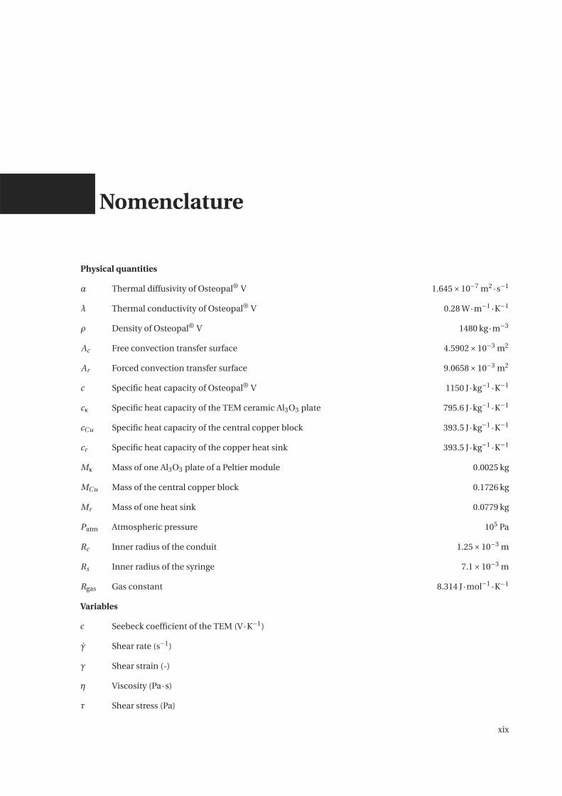
α Thermal diffusivity of Osteopal® V 1.645×10⁻⁷ m2 ·s−1
λ Thermal conductivity of Osteopal® V 0.28 W·m−1 ·K−1
ρ Density of Osteopal® V 1480 kg·m−3
Ac Free convection transfer surface 4.5902×10⁻³ m2
Ar Forced convection transfer surface 9.0658×10⁻³ m2
c Specific heat capacity of Osteopal® V 1150 J ·kg−1 ·K−1
cκ Specific heat capacity of the TEM ceramic Al3O3 plate 795.6 J ·kg−1 ·K−1
cCu Specific heat capacity of the central copper block 393.5 J ·kg−1 ·K−1
cr Specific heat capacity of the copper heat sink 393.5 J ·kg−1 ·K−1
Mκ Mass of one Al3O3 plate of a Peltier module 0.0025 kg
MCu Mass of the central copper block 0.1726 kg
Mr Mass of one heat sink 0.0779 kg
Patm Atmospheric pressure 105 Pa
Rc Inner radius of the conduit 1.25×10⁻³ m
Rs Inner radius of the syringe 7.1×10⁻³ m
Rgas Gas constant 8.314 J ·mol−1 ·K−1
Variables
ε Seebeck coefficient of the TEM (V·K−1)
γ Shear rate (s−1)
γ Shear strain (-)
η Viscosity (Pa·s)
τ Shear stress (Pa)
xix
Nomenclature
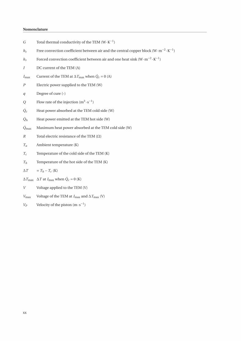
G Total thermal conductivity of the TEM (W·K−1)
hc Free convection coefficient between air and the central copper block (W·m−2 ·K−1)
hr Forced convection coefficient between air and one heat sink (W·m−2 ·K−1)
I DC current of the TEM (A)
Imax Current of the TEM at ΔTmax when Qc = 0 (A)
P Electric power supplied to the TEM (W)
q Degree of cure (-)
Q Flow rate of the injection (m3 ·s−1)
Qc Heat power absorbed at the TEM cold side (W)
Qh Heat power emitted at the TEM hot side (W)
Qmax Maximum heat power absorbed at the TEM cold side (W)
R Total electric resistance of the TEM (Ω)
Ta Ambient temperature (K)
Tc Temperature of the cold side of the TEM (K)
Th Temperature of the hot side of the TEM (K)
ΔT = Th −Tc (K)
ΔTmax ΔT at Imax when Qc = 0 (K)
V Voltage applied to the TEM (V)
Vmax Voltage of the TEM at Imax and ΔTmax (V)
VP Velocity of the piston (m·s−1)
xx
1 Problem statement
Contents
1.1 Spine health . . . . . . . . . . . . . . . . . . . . . . . . . . . . . . . . . . . . . . . . . . . . . . . . . . . 2
1.1.1 General spine anatomy . . . . . . . . . . . . . . . . . . . . . . . . . . . . . . . . . . . . . . . . 2
1.1.2 Vertebral compression fractures . . . . . . . . . . . . . . . . . . . . . . . . . . . . . . . . . . . 5
1.1.3 Proposed treatments . . . . . . . . . . . . . . . . . . . . . . . . . . . . . . . . . . . . . . . . . . 6
1.2 Percutaneous vertebroplasty . . . . . . . . . . . . . . . . . . . . . . . . . . . . . . . . . . . . . . . . . 8
1.2.1 History and current state . . . . . . . . . . . . . . . . . . . . . . . . . . . . . . . . . . . . . . . 8
1.2.2 Acrylic bone cements . . . . . . . . . . . . . . . . . . . . . . . . . . . . . . . . . . . . . . . . . 9
1.2.3 Procedure . . . . . . . . . . . . . . . . . . . . . . . . . . . . . . . . . . . . . . . . . . . . . . . . 13
1.2.4 Benefits . . . . . . . . . . . . . . . . . . . . . . . . . . . . . . . . . . . . . . . . . . . . . . . . . . 16
1.2.5 Complications and drawbacks . . . . . . . . . . . . . . . . . . . . . . . . . . . . . . . . . . . . 16
1.3 Available injection tools . . . . . . . . . . . . . . . . . . . . . . . . . . . . . . . . . . . . . . . . . . . . 17
1.3.1 Manual systems . . . . . . . . . . . . . . . . . . . . . . . . . . . . . . . . . . . . . . . . . . . . . 17
1.3.2 Mechatronic systems . . . . . . . . . . . . . . . . . . . . . . . . . . . . . . . . . . . . . . . . . . 19
1.3.3 S-Tronic project . . . . . . . . . . . . . . . . . . . . . . . . . . . . . . . . . . . . . . . . . . . . . 21
1.4 Thesis contributions and organization . . . . . . . . . . . . . . . . . . . . . . . . . . . . . . . . . . . 22
1.4.1 Thesis contributions . . . . . . . . . . . . . . . . . . . . . . . . . . . . . . . . . . . . . . . . . . 22
1.4.2 Thesis organization . . . . . . . . . . . . . . . . . . . . . . . . . . . . . . . . . . . . . . . . . . . 22
1
Chapter 1. Problem statement
1.1 Spine health
1.1.1 General spine anatomy
With an articulated bone chain, the spine represents the central pillar of the human’s trunk. At the upper end,
it must carry the head and allow its movements, while fixed to the pelvis at the lower end. It serves as a fixing
strut of hundreds of muscles and plays an important part in the posture and the locomotion. Finally, it ensures
protection of the caudal central nervous system: the spinal cord. The whole vertebral column also shows an
important vascularity.
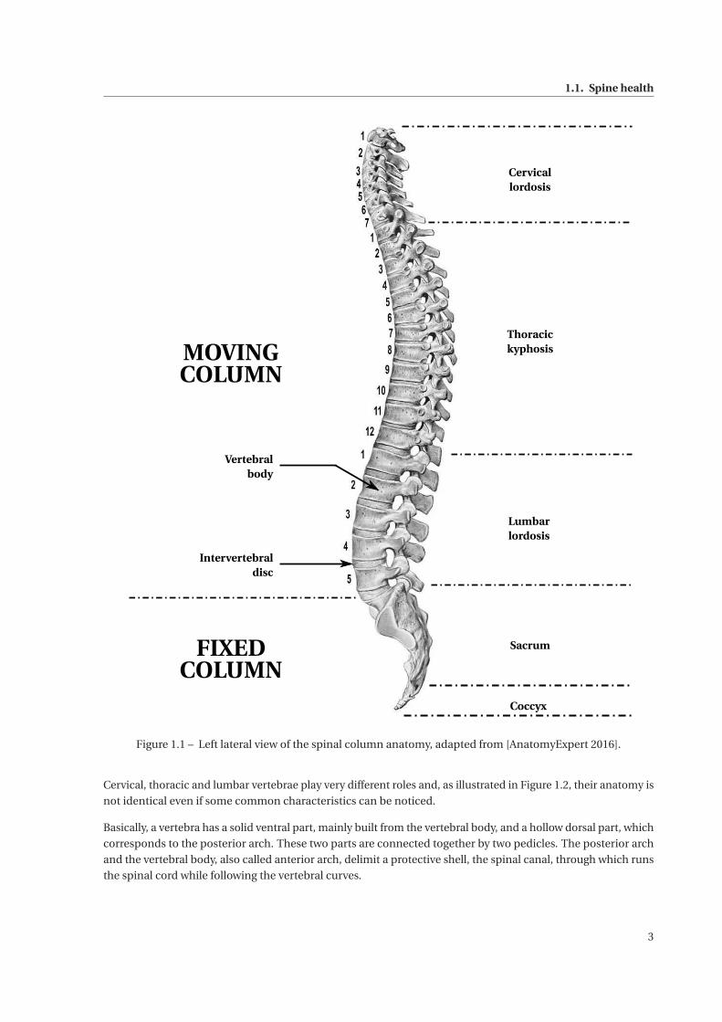
Figure 1.1 on the facing page illustrates the spine, showing a sequence of individual rigid vertebrae connected
with deformable and elastic intervertebral discs, their form and their respective dimensions. The spine can be
divided into two parts: the moving column that corresponds to the articulated part and the fixed column which
supports the moving column.
On one hand, strengthening the whole spine, the moving column presents a succession of more or less accen-
tuated physiological curvatures that defines three regions: the cervical, thoracic and lumbar columns. Each
of these segments has a specific role. The least accentuated, the cervical lordosis (convex forwards), consists
of 7 vertebrae (C1 to C7). It must support the head and allows its orientation in all directions. Mobility is
here maximum, especially in rotation. Bones, joints and muscles provide good protection, but this region
remains fragile. With 12 vertebrae (T1 to T12), the thoracic kyphosis (convex dorsally) bears the thorax that
protects vital organs, the head, and the upper limbs that are very mobile but must also allow respiratory motions.
Finally, the lumbar lordosis and its 5 vertebrae (L1 to L5) hold the trunk, and indirectly the head and the upper
limbs. Stability and strength are furthered by limiting rotation movements but by encouraging flexion-extension
movements. The acquisition of these curves is carried out during the first years of life since, in infants under
6 months, there is only a single curvature, the cervical-thoraco-lumbar curvature. The seating position and
the support of the head will match with the development of the cervical curvature. Once the standing position
is acquired, the last curve expands in order to adapt to these new constraints. These curvatures are adjusted
according to loads they support, but also to shocks they absorb.
On the other hand, the fixed column consists of the sacral kyphosis, or sacrum, which is made up of 5 fused
vertebrae, and of the coccyx, the most distal part of the spine, consisting of the fusion of 4 to 5 vertebrae
depending on the individuals. The average size of the spine varies from 70 to 75 cm in men and from 60 to 65 cm
in women, corresponding to two fifth of the stature [Standring 2008].
2
1.1. Spine health
Cervicallordosis
Thoracickyphosis
Lumbarlordosis
Sacrum
Coccyx
Vertebralbody
Intervertebraldisc
MOVINGCOLUMN
FIXEDCOLUMN
Figure 1.1 – Left lateral view of the spinal column anatomy, adapted from [AnatomyExpert 2016].
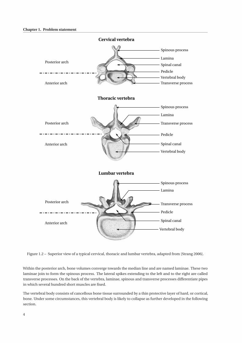
Cervical, thoracic and lumbar vertebrae play very different roles and, as illustrated in Figure 1.2, their anatomy is
not identical even if some common characteristics can be noticed.
Basically, a vertebra has a solid ventral part, mainly built from the vertebral body, and a hollow dorsal part, which
corresponds to the posterior arch. These two parts are connected together by two pedicles. The posterior arch
and the vertebral body, also called anterior arch, delimit a protective shell, the spinal canal, through which runs
the spinal cord while following the vertebral curves.
3
Chapter 1. Problem statement
Cervical vertebra
Thoracic vertebra
Lumbar vertebra
Spinous process
Lamina
Pedicle
Transverse process
Vertebral body
Spinal canal
Spinous process
Lamina
Pedicle
Transverse process
Vertebral body
Spinal canal
Spinous process
Lamina
Pedicle
Transverse process
Vertebral body
Spinal canal
Posterior arch
Anterior arch
Posterior arch
Anterior arch
Posterior arch
Anterior arch
Figure 1.2 – Superior view of a typical cervical, thoracic and lumbar vertebra, adapted from [Strang 2006].
Within the posterior arch, bone volumes converge towards the median line and are named laminae. These two
laminae join to form the spinous process. The lateral spikes extending to the left and to the right are called
transverse processes. On the back of the vertebra, laminae, spinous and transverse processes differentiate pipes
in which several hundred short muscles are fixed.
The vertebral body consists of cancellous bone tissue surrounded by a thin protective layer of hard, or cortical,
bone. Under some circumstances, this vertebral body is likely to collapse as further developed in the following
section.
4
1.1. Spine health
1.1.2 Vertebral compression fractures
The stack of vertebrae and intervertebral discs undergoes significant compression efforts. Vertebrae weakness
can cause long-term Vertebral Compression Fractures (VCF). They are characterized by a collapse or settling of
the vertebral body. This leads to the decrease of the vertebral height but also to a critical modification of the
physiological curvatures. These fractures most frequently occur in thoracic and lumbar regions, particularly
from T8 to L4 [Mathis 2006]. Severe pain associated with vertebral compression fractures worsens heavily the
quality of life and the functional abilities of the victim [Gangi 2006]. The incidence of these fractures increases
with age for both sexes while still remaining higher in women than in men [Felsenberg 2002].
Vertebral compression fractures are the most common consequence of osteoporosis. In 2009, the report of the
French National Authority for Health estimates that 85% of vertebral fractures are directly due to osteoporosis
[HAS 2009]. This disease is characterized by an important bone density loss, which weakens the bones and
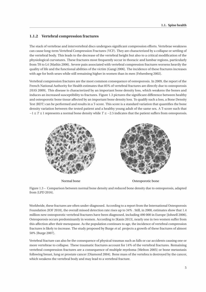
induces an increased susceptibility to fractures. Figure 1.3 pictures the significant difference between healthy
and osteoporotic bone tissue affected by an important bone density loss. To qualify such a loss, a Bone Density
Test (BDT) can be performed and results in a T-score. This score is a standard variation that quantifies the bone
density variation between the tested patient and a healthy young adult of the same sex. A T-score such that
−1 ≤ T ≤ 1 represents a normal bone density while T ≤−2.5 indicates that the patient suffers from osteoporosis.
Normal bone Osteoporotic bone
Figure 1.3 – Comparison between normal bone density and reduced bone density due to osteoporosis, adaptedfrom [LPD 2016].
Worldwide, these fractures are often under-diagnosed. According to a report from the International Osteoporosis
Foundation [IOF 2010], the overall missed detection rate rises up to 34% . Still, in 2000, estimates show that 1.4
million new osteoporotic vertebral fractures have been diagnosed, including 490 000 in Europe [Johnell 2006].
Osteoporosis occurs predominantly in women. According to [Kanis 2013], nearly one in two women suffer from
this affection after their menopause. As the population continues to age, the incidence of vertebral compression
fractures is likely to increase. The study proposed by Burge et al. projects a growth of these fractures of almost
50% [Burge 2007].
Vertebral fracture can also be the consequence of physical traumas such as falls or car accidents causing one or
more vertebrae to collapse. These traumatic fractures account for 14% of the vertebral fractures. Remaining
vertebral compression fractures are a consequence of multiple myeloma [Melton 2005] or bone metastasis
following breast, lung or prostate cancer [Diamond 2004]. Bone mass of the vertebra is destroyed by the cancer,
which weakens the vertebral body and may lead to a vertebral fracture.
5
Chapter 1. Problem statement
1.1.3 Proposed treatments
In light of this growing public health problem, various treatments are available starting from simple conservative
to surgical solutions. These different medical cares will be detailed and discussed in the following subsections.
1.1.3.1 Conservative treatment
The treatment of vertebral fractures is usually conservative. The patient is strapped into a back brace to ensure
the support of the spine and asked to remain in a lying position [Klazen 2010]. Pain is relieved by a drug
administration including narcotic analgesics. Physiotherapy sessions and dietary supplements can complete
this treatment. Until recently, this option remained the only considered, even if pain could last for months.
Because of such a long immobilization, it may also have psychological consequences for the patient.
1.1.3.2 Vertebroplasty and its derivatives
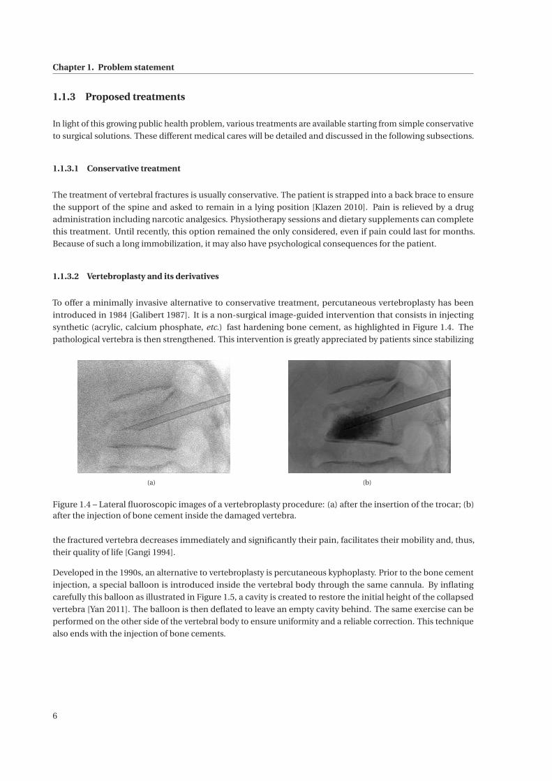
To offer a minimally invasive alternative to conservative treatment, percutaneous vertebroplasty has been
introduced in 1984 [Galibert 1987]. It is a non-surgical image-guided intervention that consists in injecting
synthetic (acrylic, calcium phosphate, etc.) fast hardening bone cement, as highlighted in Figure 1.4. The
pathological vertebra is then strengthened. This intervention is greatly appreciated by patients since stabilizing
(a) (b)
Figure 1.4 – Lateral fluoroscopic images of a vertebroplasty procedure: (a) after the insertion of the trocar; (b)after the injection of bone cement inside the damaged vertebra.
the fractured vertebra decreases immediately and significantly their pain, facilitates their mobility and, thus,
their quality of life [Gangi 1994].
Developed in the 1990s, an alternative to vertebroplasty is percutaneous kyphoplasty. Prior to the bone cement
injection, a special balloon is introduced inside the vertebral body through the same cannula. By inflating
carefully this balloon as illustrated in Figure 1.5, a cavity is created to restore the initial height of the collapsed
vertebra [Yan 2011]. The balloon is then deflated to leave an empty cavity behind. The same exercise can be
performed on the other side of the vertebral body to ensure uniformity and a reliable correction. This technique
also ends with the injection of bone cements.
6
1.1. Spine health
Figure 1.5 – Illustration of a kyphoplasty procedure, from [Center 2015].
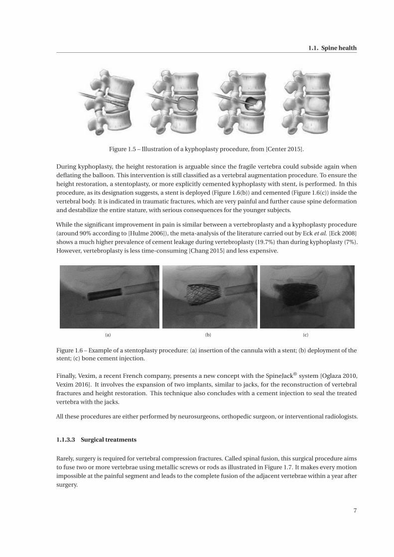
During kyphoplasty, the height restoration is arguable since the fragile vertebra could subside again when
deflating the balloon. This intervention is still classified as a vertebral augmentation procedure. To ensure the
height restoration, a stentoplasty, or more explicitly cemented kyphoplasty with stent, is performed. In this
procedure, as its designation suggests, a stent is deployed (Figure 1.6(b)) and cemented (Figure 1.6(c)) inside the
vertebral body. It is indicated in traumatic fractures, which are very painful and further cause spine deformation
and destabilize the entire stature, with serious consequences for the younger subjects.
While the significant improvement in pain is similar between a vertebroplasty and a kyphoplasty procedure
(around 90% according to [Hulme 2006]), the meta-analysis of the literature carried out by Eck et al. [Eck 2008]
shows a much higher prevalence of cement leakage during vertebroplasty (19.7%) than during kyphoplasty (7%).
However, vertebroplasty is less time-consuming [Chang 2015] and less expensive.
(a) (b) (c)
Figure 1.6 – Example of a stentoplasty procedure: (a) insertion of the cannula with a stent; (b) deployment of thestent; (c) bone cement injection.
Finally, Vexim, a recent French company, presents a new concept with the SpineJack® system [Oglaza 2010,
Vexim 2016]. It involves the expansion of two implants, similar to jacks, for the reconstruction of vertebral
fractures and height restoration. This technique also concludes with a cement injection to seal the treated
vertebra with the jacks.
All these procedures are either performed by neurosurgeons, orthopedic surgeon, or interventional radiologists.
1.1.3.3 Surgical treatments
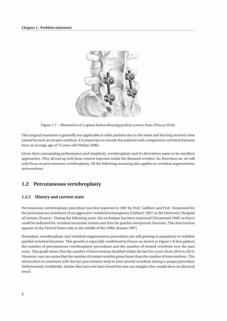
Rarely, surgery is required for vertebral compression fractures. Called spinal fusion, this surgical procedure aims
to fuse two or more vertebrae using metallic screws or rods as illustrated in Figure 1.7. It makes every motion
impossible at the painful segment and leads to the complete fusion of the adjacent vertebrae within a year after
surgery.
7
Chapter 1. Problem statement
Figure 1.7 – Illustration of a spinal fusion showing pedicle screws, from [Pincus 2016].
This surgical treatment is generally not applicable to older patients due to the stress and the long recovery time
caused by such an invasive method. It is important to remark that patients with compression vertebral fractures
have an average age of 75 years old [Hulme 2006].
Given their outstanding performance and simplicity, vertebroplasty and its derivatives seem to be excellent
approaches. They all end up with bone cement injection inside the diseased vertebra. So, from here on, we will
only focus on percutaneous vertebroplasty. All the following reasoning also applies to vertebral augmentation
interventions.
1.2 Percutaneous vertebroplasty
1.2.1 History and current state
Percutaneous vertebroplasty procedure was first reported in 1987 by Prof. Galibert and Prof. Deramond for
the percutaneous treatment of an aggressive vertebral hemangioma [Galibert 1987] at the University Hospital
of Amiens (France). During the following years, this technique has been improved [Deramond 1998] so that it
could be indicated for vertebral metastatic lesions and then for painful osteoporotic fractures. This intervention
appears in the United States only in the middle of the 1990s [Jensen 1997].
Nowadays, vertebroplasty and vertebral augmentation procedures are still gaining in popularity to stabilize
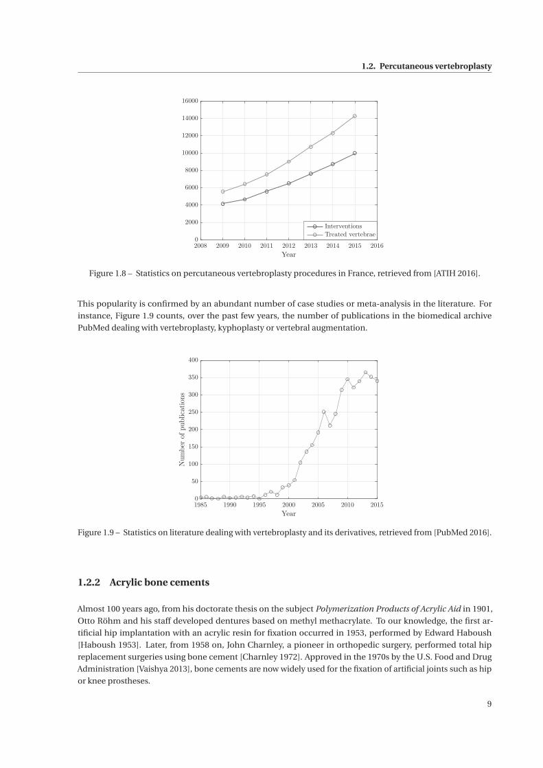
painful vertebral fractures. This growth is especially confirmed in France as shown in Figure 1.8 that gathers
the number of percutaneous vertebroplasty procedures and the number of treated vertebrae over the past
years. This graph shows that the number of interventions doubled within the last five years (from 2010 to 2015).
Moreover, one can notice that the number of treated vertebra grows faster than the number of interventions. This
observation is consistent with the fact practitioners tend to treat several vertebrae during a unique procedure.
Unfortunately, worldwide, similar data have not been found but one can imagine they would show an identical
trend.
8
1.2. Percutaneous vertebroplasty
2008 2009 2010 2011 2012 2013 2014 2015 2016
Year
0
2000
4000
6000
8000
10000
12000
14000
16000
Interventions
Treated vertebrae
Figure 1.8 – Statistics on percutaneous vertebroplasty procedures in France, retrieved from [ATIH 2016].
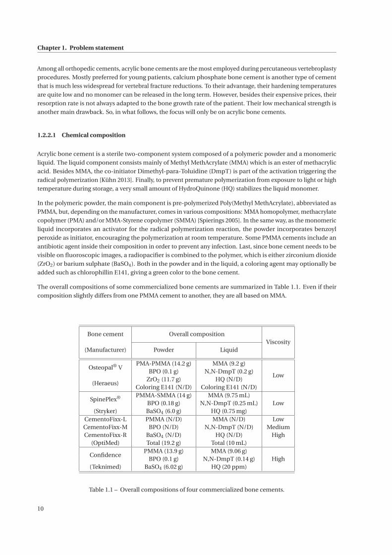
This popularity is confirmed by an abundant number of case studies or meta-analysis in the literature. For
instance, Figure 1.9 counts, over the past few years, the number of publications in the biomedical archive
PubMed dealing with vertebroplasty, kyphoplasty or vertebral augmentation.
1985 1990 1995 2000 2005 2010 2015
Year
0
50
100
150
200
250
300
350
400
Numberofpublications
Figure 1.9 – Statistics on literature dealing with vertebroplasty and its derivatives, retrieved from [PubMed 2016].
1.2.2 Acrylic bone cements
Almost 100 years ago, from his doctorate thesis on the subject Polymerization Products of Acrylic Aid in 1901,
Otto Röhm and his staff developed dentures based on methyl methacrylate. To our knowledge, the first ar-
tificial hip implantation with an acrylic resin for fixation occurred in 1953, performed by Edward Haboush
[Haboush 1953]. Later, from 1958 on, John Charnley, a pioneer in orthopedic surgery, performed total hip
replacement surgeries using bone cement [Charnley 1972]. Approved in the 1970s by the U.S. Food and Drug
Administration [Vaishya 2013], bone cements are now widely used for the fixation of artificial joints such as hip
or knee prostheses.
9
Chapter 1. Problem statement
Among all orthopedic cements, acrylic bone cements are the most employed during percutaneous vertebroplasty
procedures. Mostly preferred for young patients, calcium phosphate bone cement is another type of cement
that is much less widespread for vertebral fracture reductions. To their advantage, their hardening temperatures
are quite low and no monomer can be released in the long term. However, besides their expensive prices, their
resorption rate is not always adapted to the bone growth rate of the patient. Their low mechanical strength is
another main drawback. So, in what follows, the focus will only be on acrylic bone cements.
1.2.2.1 Chemical composition
Acrylic bone cement is a sterile two-component system composed of a polymeric powder and a monomeric
liquid. The liquid component consists mainly of Methyl MethAcrylate (MMA) which is an ester of methacrylic
acid. Besides MMA, the co-initiator Dimethyl-para-Toluidine (DmpT) is part of the activation triggering the
radical polymerization [Kühn 2013]. Finally, to prevent premature polymerization from exposure to light or high
temperature during storage, a very small amount of HydroQuinone (HQ) stabilizes the liquid monomer.
In the polymeric powder, the main component is pre-polymerized Poly(Methyl MethAcrylate), abbreviated as
PMMA, but, depending on the manufacturer, comes in various compositions: MMA homopolymer, methacrylate
copolymer (PMA) and/or MMA-Styrene copolymer (SMMA) [Spierings 2005]. In the same way, as the monomeric
liquid incorporates an activator for the radical polymerization reaction, the powder incorporates benzoyl
peroxide as initiator, encouraging the polymerization at room temperature. Some PMMA cements include an
antibiotic agent inside their composition in order to prevent any infection. Last, since bone cement needs to be
visible on fluoroscopic images, a radiopacifier is combined to the polymer, which is either zirconium dioxide
(ZrO2) or barium sulphate (BaSO4). Both in the powder and in the liquid, a coloring agent may optionally be
added such as chlorophillin E141, giving a green color to the bone cement.
The overall compositions of some commercialized bone cements are summarized in Table 1.1. Even if their
composition slightly differs from one PMMA cement to another, they are all based on MMA.
Bone cement Overall compositionViscosity
(Manufacturer) Powder Liquid
Osteopal® VPMA-PMMA (14.2 g) MMA (9.2 g)
LowBPO (0.1 g) N,N-DmpT (0.2 g)
(Heraeus)ZrO2 (11.7 g) HQ (N/D)
Coloring E141 (N/D) Coloring E141 (N/D)
SpinePlex® PMMA-SMMA (14 g) MMA (9.75 mL)LowBPO (0.18 g) N,N-DmpT (0.25 mL)
(Stryker) BaSO4 (6.0 g) HQ (0.75 mg)CementoFixx-L PMMA (N/D) MMA (N/D) LowCementoFixx-M BPO (N/D) N,N-DmpT (N/D) MediumCementoFixx-R BaSO4 (N/D) HQ (N/D) High
(OptiMed) Total (19.2 g) Total (10 mL)
ConfidencePMMA (13.9 g) MMA (9.06 g)
HighBPO (0.1 g) N,N-DmpT (0.14 g)(Teknimed) BaSO4 (6.02 g) HQ (20 ppm)
Table 1.1 – Overall compositions of four commercialized bone cements.
10
1.2. Percutaneous vertebroplasty
Especially selected for their excellent mechanical strength, acrylic bone cements can show high variable vis-
cosities, depending on their composition. They can be classified into three categories: low-, medium- and
high-viscosity PMMA cements. While their different behavior clearly depends on the bone cement composition,
manufacturers do not provide any viscosity measurement or quantification. Generally, for vertebroplasty proce-
dures, low-viscosity bone cements are preferred since their mixing and injection are more convenient, even if
leakage risks are higher.
1.2.2.2 Handling properties
As soon as both components come into contact, the PMMA evolution follows four successive phases, named as
handling phases.
Mixing phase This phase starts as soon as the powder and the liquid monomer are thoroughly mixed using an
appropriate tool, triggering the polymerization reaction. The very few and short polymer chains that are formed
are very mobile. At the end of this stage, when a homogeneous dough is obtained, the powder is fully dissolved
in the liquid and the bone cement is relatively runny. This mixing step will be further detailed in section 1.2.3
where a vertebroplasty procedure is fully described.
Waiting phase Also called doughing time, this phase of one to three minutes is recommended by manufacturers
so that the bone cement viscosity increases slowly (formation of polymer chains). When the cement does no
longer stick to the surgical glove, the viscosity is suitable for handling. The notion of viscosity, description of the
hardening of a fluid or of its ability to flow, will further be developed in Chapter 2.
Application phase During this period, the physician can inject the bone cement inside the damaged vertebra.
Viscosity increases and the intervention must be finished by the end of this working phase.
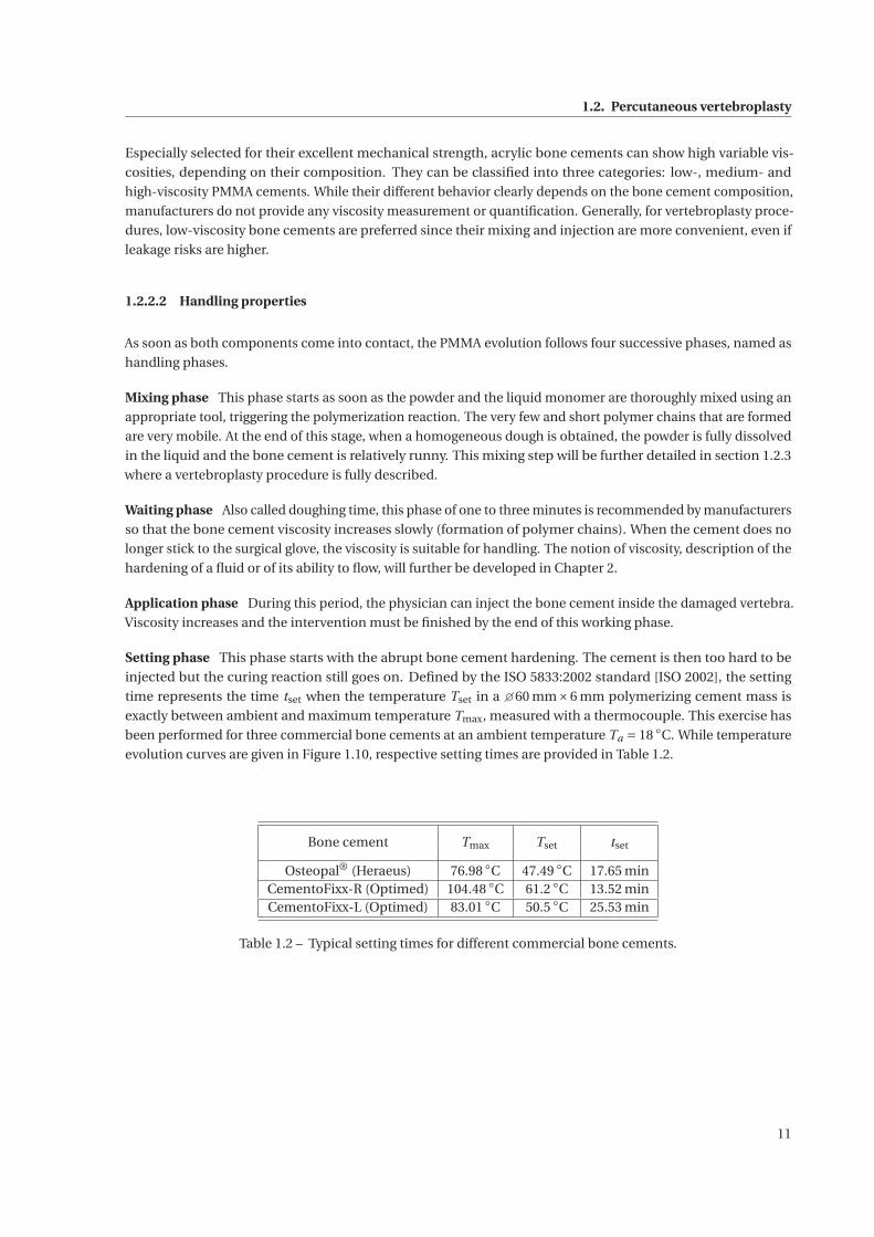
Setting phase This phase starts with the abrupt bone cement hardening. The cement is then too hard to be
injected but the curing reaction still goes on. Defined by the ISO 5833:2002 standard [ISO 2002], the setting
time represents the time tset when the temperature Tset in a �60 mm×6 mm polymerizing cement mass is
exactly between ambient and maximum temperature Tmax, measured with a thermocouple. This exercise has
been performed for three commercial bone cements at an ambient temperature Ta = 18 ◦C. While temperature
evolution curves are given in Figure 1.10, respective setting times are provided in Table 1.2.
Bone cement Tmax Tset tset
Osteopal® (Heraeus) 76.98 ◦C 47.49 ◦C 17.65 minCementoFixx-R (Optimed) 104.48 ◦C 61.2 ◦C 13.52 minCementoFixx-L (Optimed) 83.01 ◦C 50.5 ◦C 25.53 min
Table 1.2 – Typical setting times for different commercial bone cements.
11
Chapter 1. Problem statement
0 5 10 15 20 25 30 35 40
Time (min)
0
20
40
60
80
100
120
Temperature(◦C)
Osteopal V
CementoFixx-R
CementoFixx-L
Figure 1.10 – Temperature evolution curves where time zero is the beginning of the mixing phase.
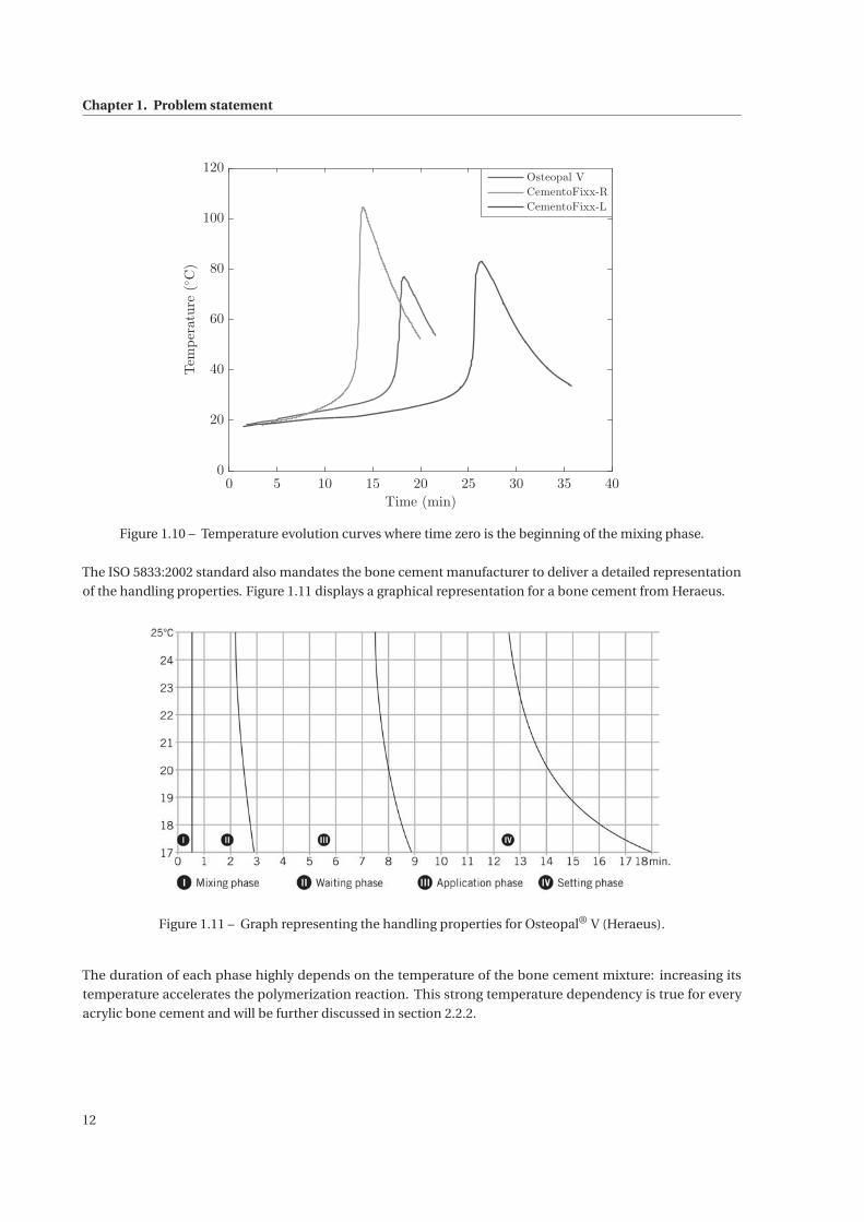
The ISO 5833:2002 standard also mandates the bone cement manufacturer to deliver a detailed representation
of the handling properties. Figure 1.11 displays a graphical representation for a bone cement from Heraeus.
Figure 1.11 – Graph representing the handling properties for Osteopal® V (Heraeus).
The duration of each phase highly depends on the temperature of the bone cement mixture: increasing its
temperature accelerates the polymerization reaction. This strong temperature dependency is true for every
acrylic bone cement and will be further discussed in section 2.2.2.
12
1.2. Percutaneous vertebroplasty
1.2.3 Procedure
In this section, a usual percutaneous vertebroplasty procedure will be described. Before any intervention, the
patient receives a preoperative assessment combining X-ray imaging and magnetic resonance imaging (MRI)
[Gangi 2010] in order to have an optimal contrast for both bones and soft tissues.
Patient setup The patient is, most of the time, placed in prone position on the table of the imaging device. For
cervical fractures only, patients are settled in supine position. Commonly, two imaging devices are combined: a
Computed Tomography scanner (CT-scan) for its high spatial resolution and an X-ray fluoroscope which is a
mobile radiography equipment that can be rotated around the table [Gangi 1994].
In general, patients receive local anesthesia with mild sedation and analgesia. Only for some personal conve-
nience or for the treatment of several fractures at the same time, general anesthesia is administered.
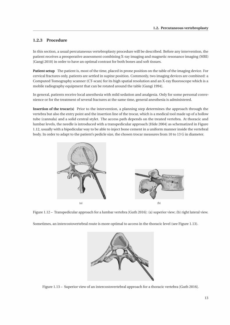
Insertion of the trocar(s) Prior to the intervention, a planning step determines the approach through the
vertebra but also the entry point and the insertion line of the trocar, which is a medical tool made up of a hollow
tube (cannula) and a solid central stylet. The access path depends on the treated vertebra. At thoracic and
lumbar levels, the needle is introduced with a transpedicular approach [Hide 2004] as schematized in Figure
1.12, usually with a bipedicular way to be able to inject bone cement in a uniform manner inside the vertebral
body. In order to adapt to the patient’s pedicle size, the chosen trocar measures from 10 to 13 G in diameter.
(a) (b)
Figure 1.12 – Transpedicular approach for a lumbar vertebra [Guth 2016]: (a) superior view; (b) right lateral view.
Sometimes, an intercostovertebral route is more optimal to access in the thoracic level (see Figure 1.13).
Figure 1.13 – Superior view of an intercostovertebral approach for a thoracic vertebra [Guth 2016].
13
Chapter 1. Problem statement
For the few cervical procedures, a unilateral anterolateral approach is recommended with the use of thinner
needles, from 13 to 15G in diameter.
Once the entry point is defined, a small incision is made. The needle is hammered inside the vertebra. The
scanner allows the precise guidance of the tool [Gangi 2006] amid the adjacent structures (vascular, neurological
and visceral) on the planned trajectory. However, images can only be acquired in a unique plane, potentially
slightly inclined. Exposure time to X-rays is relatively low during this stage because the acquisition flow is not
continuous and the medical staff can step out the X-ray area when the acquisition of a new image is required.
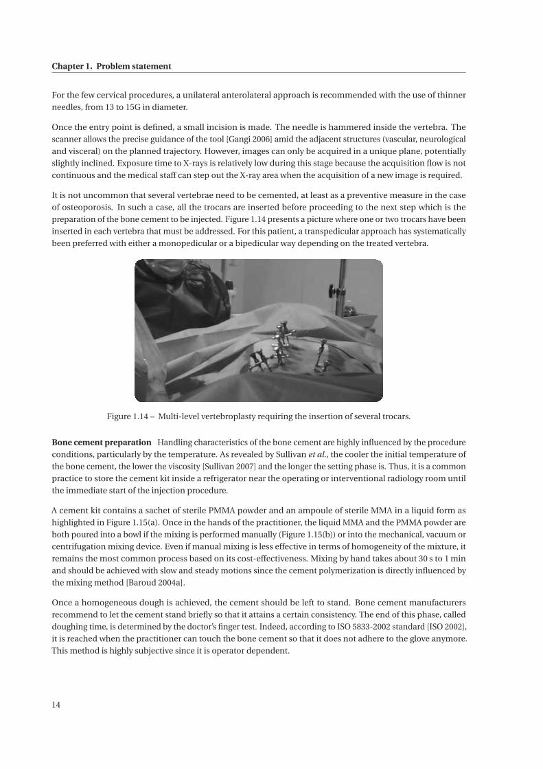
It is not uncommon that several vertebrae need to be cemented, at least as a preventive measure in the case
of osteoporosis. In such a case, all the trocars are inserted before proceeding to the next step which is the
preparation of the bone cement to be injected. Figure 1.14 presents a picture where one or two trocars have been
inserted in each vertebra that must be addressed. For this patient, a transpedicular approach has systematically
been preferred with either a monopedicular or a bipedicular way depending on the treated vertebra.
Figure 1.14 – Multi-level vertebroplasty requiring the insertion of several trocars.
Bone cement preparation Handling characteristics of the bone cement are highly influenced by the procedure
conditions, particularly by the temperature. As revealed by Sullivan et al., the cooler the initial temperature of
the bone cement, the lower the viscosity [Sullivan 2007] and the longer the setting phase is. Thus, it is a common
practice to store the cement kit inside a refrigerator near the operating or interventional radiology room until
the immediate start of the injection procedure.
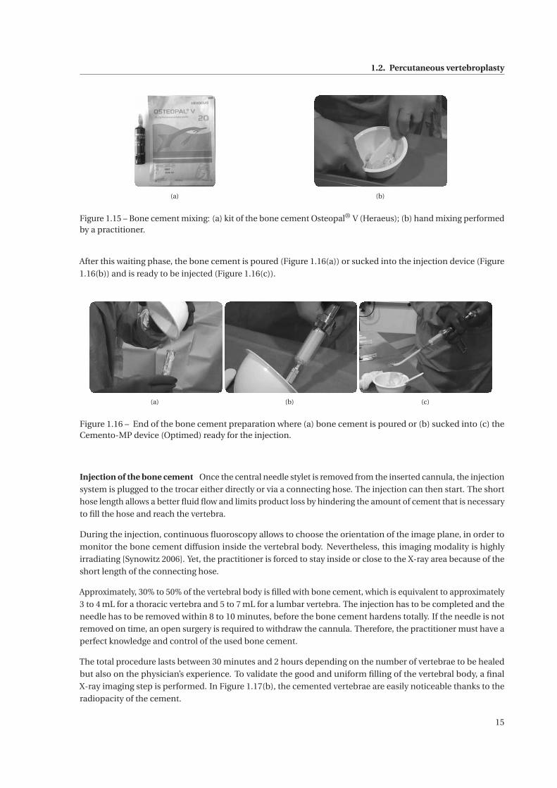
A cement kit contains a sachet of sterile PMMA powder and an ampoule of sterile MMA in a liquid form as
highlighted in Figure 1.15(a). Once in the hands of the practitioner, the liquid MMA and the PMMA powder are
both poured into a bowl if the mixing is performed manually (Figure 1.15(b)) or into the mechanical, vacuum or
centrifugation mixing device. Even if manual mixing is less effective in terms of homogeneity of the mixture, it
remains the most common process based on its cost-effectiveness. Mixing by hand takes about 30 s to 1 min
and should be achieved with slow and steady motions since the cement polymerization is directly influenced by
the mixing method [Baroud 2004a].
Once a homogeneous dough is achieved, the cement should be left to stand. Bone cement manufacturers
recommend to let the cement stand briefly so that it attains a certain consistency. The end of this phase, called
doughing time, is determined by the doctor’s finger test. Indeed, according to ISO 5833-2002 standard [ISO 2002],
it is reached when the practitioner can touch the bone cement so that it does not adhere to the glove anymore.
This method is highly subjective since it is operator dependent.
14
1.2. Percutaneous vertebroplasty
(a) (b)
Figure 1.15 – Bone cement mixing: (a) kit of the bone cement Osteopal® V (Heraeus); (b) hand mixing performedby a practitioner.
After this waiting phase, the bone cement is poured (Figure 1.16(a)) or sucked into the injection device (Figure
1.16(b)) and is ready to be injected (Figure 1.16(c)).
(a) (b) (c)
Figure 1.16 – End of the bone cement preparation where (a) bone cement is poured or (b) sucked into (c) theCemento-MP device (Optimed) ready for the injection.
Injection of the bone cement Once the central needle stylet is removed from the inserted cannula, the injection
system is plugged to the trocar either directly or via a connecting hose. The injection can then start. The short
hose length allows a better fluid flow and limits product loss by hindering the amount of cement that is necessary
to fill the hose and reach the vertebra.
During the injection, continuous fluoroscopy allows to choose the orientation of the image plane, in order to
monitor the bone cement diffusion inside the vertebral body. Nevertheless, this imaging modality is highly
irradiating [Synowitz 2006]. Yet, the practitioner is forced to stay inside or close to the X-ray area because of the
short length of the connecting hose.
Approximately, 30% to 50% of the vertebral body is filled with bone cement, which is equivalent to approximately
3 to 4 mL for a thoracic vertebra and 5 to 7 mL for a lumbar vertebra. The injection has to be completed and the
needle has to be removed within 8 to 10 minutes, before the bone cement hardens totally. If the needle is not
removed on time, an open surgery is required to withdraw the cannula. Therefore, the practitioner must have a
perfect knowledge and control of the used bone cement.
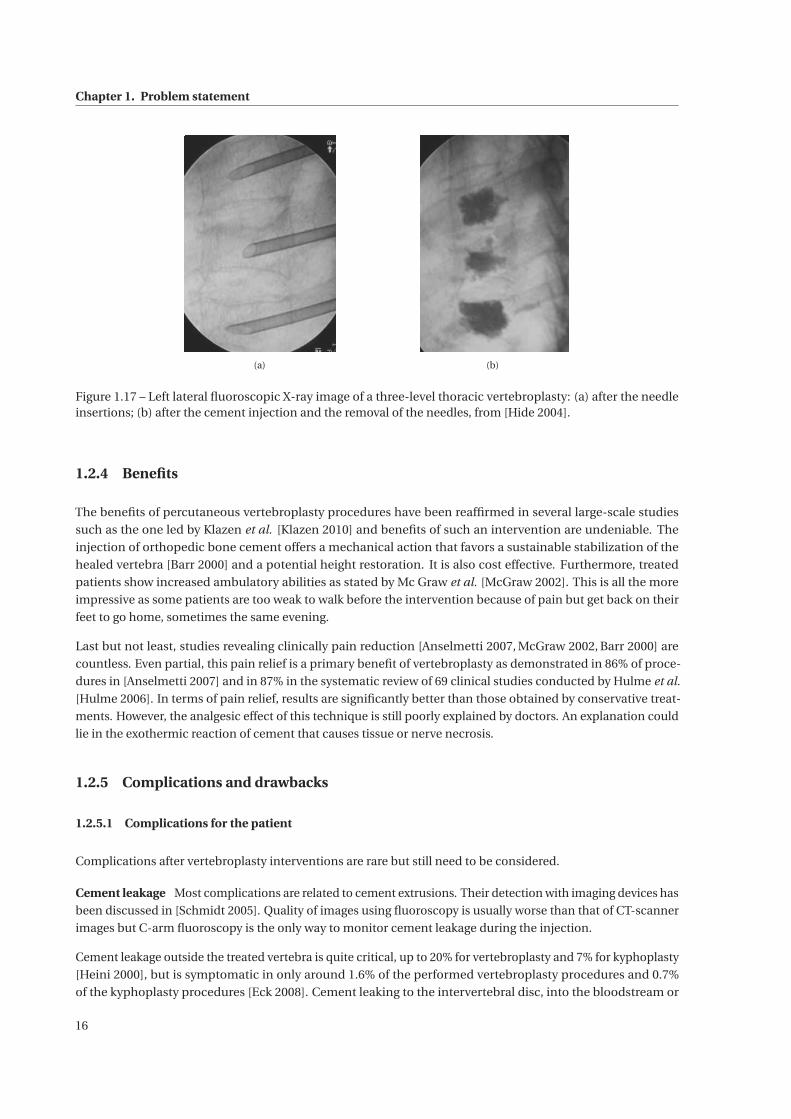
The total procedure lasts between 30 minutes and 2 hours depending on the number of vertebrae to be healed
but also on the physician’s experience. To validate the good and uniform filling of the vertebral body, a final
X-ray imaging step is performed. In Figure 1.17(b), the cemented vertebrae are easily noticeable thanks to the
radiopacity of the cement.
15
Chapter 1. Problem statement
(a) (b)
Figure 1.17 – Left lateral fluoroscopic X-ray image of a three-level thoracic vertebroplasty: (a) after the needleinsertions; (b) after the cement injection and the removal of the needles, from [Hide 2004].
1.2.4 Benefits
The benefits of percutaneous vertebroplasty procedures have been reaffirmed in several large-scale studies
such as the one led by Klazen et al. [Klazen 2010] and benefits of such an intervention are undeniable. The
injection of orthopedic bone cement offers a mechanical action that favors a sustainable stabilization of the
healed vertebra [Barr 2000] and a potential height restoration. It is also cost effective. Furthermore, treated
patients show increased ambulatory abilities as stated by Mc Graw et al. [McGraw 2002]. This is all the more
impressive as some patients are too weak to walk before the intervention because of pain but get back on their
feet to go home, sometimes the same evening.
Last but not least, studies revealing clinically pain reduction [Anselmetti 2007, McGraw 2002, Barr 2000] are
countless. Even partial, this pain relief is a primary benefit of vertebroplasty as demonstrated in 86% of proce-
dures in [Anselmetti 2007] and in 87% in the systematic review of 69 clinical studies conducted by Hulme et al.
[Hulme 2006]. In terms of pain relief, results are significantly better than those obtained by conservative treat-
ments. However, the analgesic effect of this technique is still poorly explained by doctors. An explanation could
lie in the exothermic reaction of cement that causes tissue or nerve necrosis.
1.2.5 Complications and drawbacks
1.2.5.1 Complications for the patient
Complications after vertebroplasty interventions are rare but still need to be considered.
Cement leakage Most complications are related to cement extrusions. Their detection with imaging devices has
been discussed in [Schmidt 2005]. Quality of images using fluoroscopy is usually worse than that of CT-scanner
images but C-arm fluoroscopy is the only way to monitor cement leakage during the injection.
Cement leakage outside the treated vertebra is quite critical, up to 20% for vertebroplasty and 7% for kyphoplasty
[Heini 2000], but is symptomatic in only around 1.6% of the performed vertebroplasty procedures and 0.7%
of the kyphoplasty procedures [Eck 2008]. Cement leaking to the intervertebral disc, into the bloodstream or
16
1.3. Available injection tools
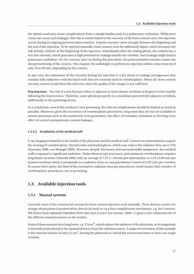
the spinal canal may cause complications from a simple lumbar pain to a pulmonary embolism. While poor
vision can cause such leakages, this risk is mostly linked to the viscosity of the bone cement since the injection
occurs during its ongoing polymerization reaction. Cement viscosity varies strongly between the beginning and
the end of the injection. To be injected manually, bone cement must be sufficiently liquid, which increases the
risk of leaks. Indeed, at the beginning of the injection, immediately after the mixing phase, the cement has a
very low viscosity, which generates a high potential for leakage outside the vertebra. Such leakage might lead to
pulmonary embolism. On the contrary, later on during this procedure, the polymerization reaction causes the
abrupt hardening of the cement. This requires the radiologist to perform its injection within a time interval of
only 10 to 20 min, depending on the cement.
In any case, the estimation of the viscosity during the injection is a key factor in leakage management that
remains fully subjective with the hand tools that are currently used in vertebroplasty. Above all, bone cement
viscosity control would limit this risk even when the quality of the images is not sufficient.
New fractures The risk of a new fracture either to adjacent or more distant vertebrae is frequent in the months
following the intervention. Therefore, some physicians prefer to consolidate preventively adjacent vertebrae,
additionally to the pathological one.
As a conclusion, even if this method is very promising, the risks of complications should be limited as much as
possible. Moreover, given the recentness of vertebroplasty procedures, long-term data are not yet available to
answer questions such as the exothermic heat generation, the effect of monomer emissions or the long-term
effect of a priori asymptomatic cement leakages.
1.2.5.2 Irradiation of the medical staff
X-ray imaging is harmful to the health of the physician and his medical staff. Current recommendations require
the wearing of a leaded apron, thyroid collar and leaded gloves, which may reduce the radiation dose up to 75%
[Synowitz 2006, von Wrangel 2009]. However, despite this heavy and uncomfortable equipment, the medical
staff is exposed to significant radiation. Under fluoroscopy assistance, percutaneous vertebroplasty requires
long beam-on times [Harstall 2005] with an average of 7.97±1.96 min per intervention or 2.23±0.89 min per
treated vertebrae which corresponds to a radiation dose on one practitioner’s hand of 0.107 mSv per vertebra.
To ensure their safety, the limit of the cumulative radiation dose per practitioner could restrict their number of
vertebroplasty procedures, yet so promising.
1.3 Available injection tools
1.3.1 Manual systems
Currently, most of the commercial systems for bone cement injection work manually. These devices consist of a
syringe whose piston is pushed either directly by hand or via a force amplification mechanism, e.g. the Cemento-
MP device from Optimed [OptiMed 2016] that uses a screw-nut system. Table 1.3 gives a non-exhaustive list of
the different manual systems on the market.
Some of these systems have long hoses, e.g. X’tens®, which reduce the radiation of the physician, as its magnitude
is inversely proportional to the squared distance from the radiation source. A major inconvenient of this example
is the internal volume of only 2.5 cm3, forcing the physician to reload the tool several times to treat one single
vertebra.
17
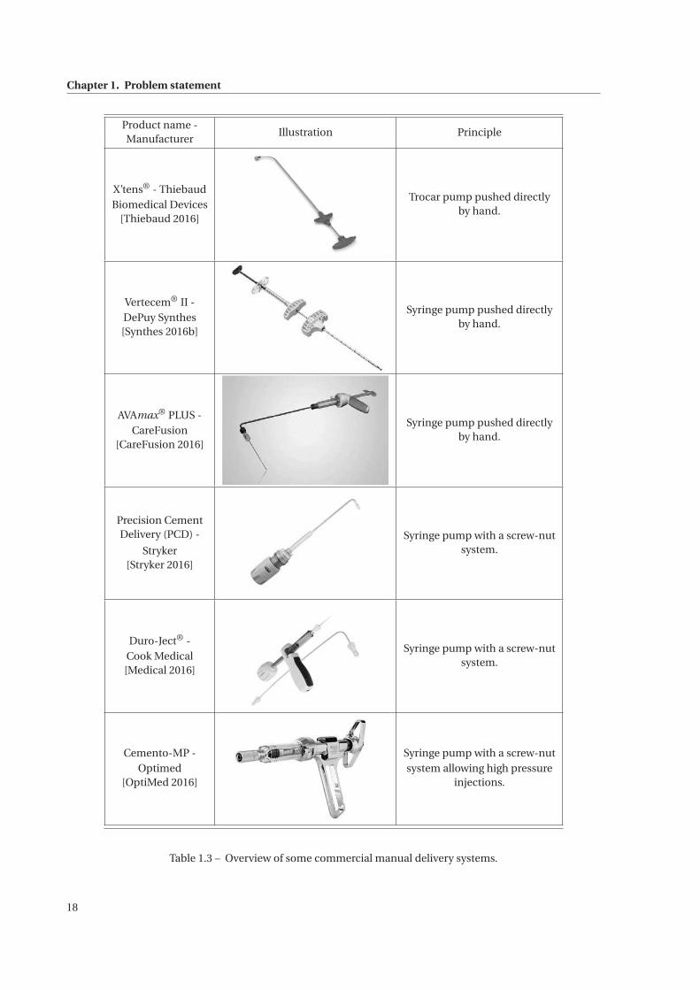
Chapter 1. Problem statement
Product name -Manufacturer
Illustration Principle
X’tens® - ThiebaudBiomedical Devices
[Thiebaud 2016]
Trocar pump pushed directlyby hand.
Vertecem® II -DePuy Synthes[Synthes 2016b]
Syringe pump pushed directlyby hand.
AVAmax® PLUS -CareFusion
[CareFusion 2016]
Syringe pump pushed directlyby hand.
Precision CementDelivery (PCD) -
Stryker[Stryker 2016]
Syringe pump with a screw-nutsystem.
Duro-Ject® -Cook Medical[Medical 2016]
Syringe pump with a screw-nutsystem.
Cemento-MP -Optimed
[OptiMed 2016]
Syringe pump with a screw-nutsystem allowing high pressure
injections.
Table 1.3 – Overview of some commercial manual delivery systems.
18
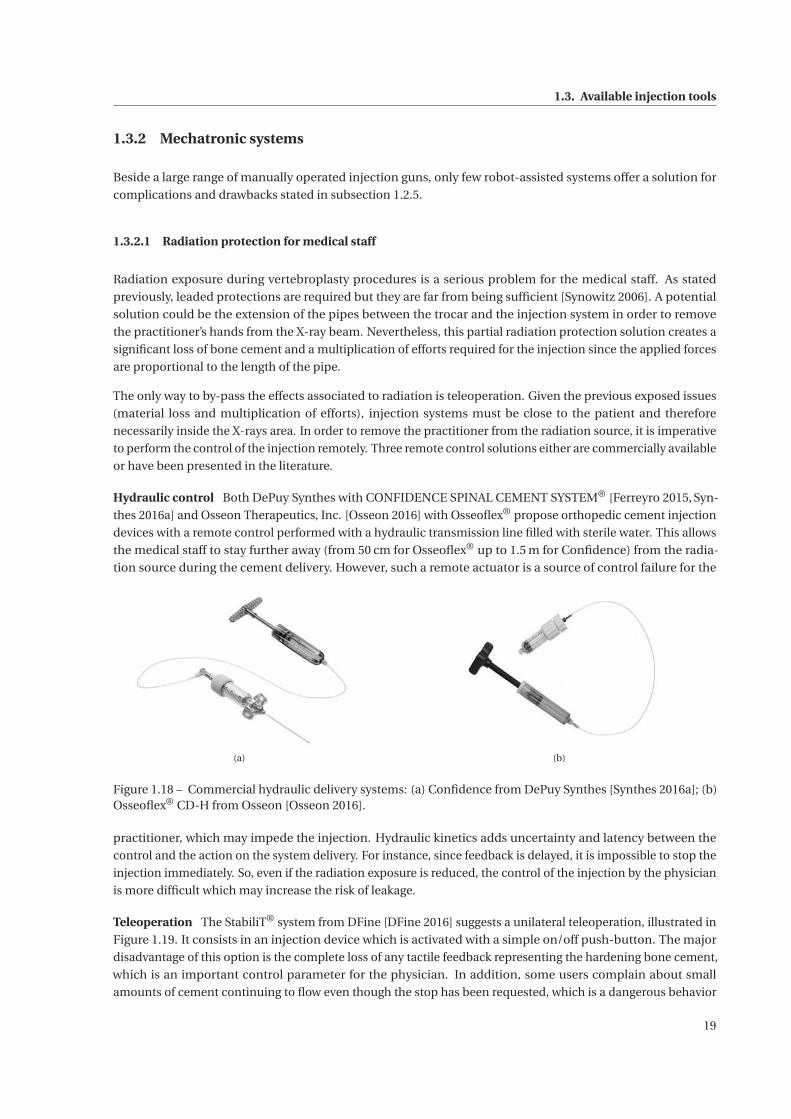
1.3. Available injection tools
1.3.2 Mechatronic systems
Beside a large range of manually operated injection guns, only few robot-assisted systems offer a solution for
complications and drawbacks stated in subsection 1.2.5.
1.3.2.1 Radiation protection for medical staff
Radiation exposure during vertebroplasty procedures is a serious problem for the medical staff. As stated
previously, leaded protections are required but they are far from being sufficient [Synowitz 2006]. A potential
solution could be the extension of the pipes between the trocar and the injection system in order to remove
the practitioner’s hands from the X-ray beam. Nevertheless, this partial radiation protection solution creates a
significant loss of bone cement and a multiplication of efforts required for the injection since the applied forces
are proportional to the length of the pipe.
The only way to by-pass the effects associated to radiation is teleoperation. Given the previous exposed issues
(material loss and multiplication of efforts), injection systems must be close to the patient and therefore
necessarily inside the X-rays area. In order to remove the practitioner from the radiation source, it is imperative
to perform the control of the injection remotely. Three remote control solutions either are commercially available
or have been presented in the literature.
Hydraulic control Both DePuy Synthes with CONFIDENCE SPINAL CEMENT SYSTEM® [Ferreyro 2015, Syn-
thes 2016a] and Osseon Therapeutics, Inc. [Osseon 2016] with Osseoflex® propose orthopedic cement injection
devices with a remote control performed with a hydraulic transmission line filled with sterile water. This allows
the medical staff to stay further away (from 50 cm for Osseoflex® up to 1.5 m for Confidence) from the radia-
tion source during the cement delivery. However, such a remote actuator is a source of control failure for the
(a) (b)
Figure 1.18 – Commercial hydraulic delivery systems: (a) Confidence from DePuy Synthes [Synthes 2016a]; (b)Osseoflex® CD-H from Osseon [Osseon 2016].
practitioner, which may impede the injection. Hydraulic kinetics adds uncertainty and latency between the
control and the action on the system delivery. For instance, since feedback is delayed, it is impossible to stop the
injection immediately. So, even if the radiation exposure is reduced, the control of the injection by the physician
is more difficult which may increase the risk of leakage.
Teleoperation The StabiliT® system from DFine [DFine 2016] suggests a unilateral teleoperation, illustrated in
Figure 1.19. It consists in an injection device which is activated with a simple on/off push-button. The major
disadvantage of this option is the complete loss of any tactile feedback representing the hardening bone cement,
which is an important control parameter for the physician. In addition, some users complain about small
amounts of cement continuing to flow even though the stop has been requested, which is a dangerous behavior
19
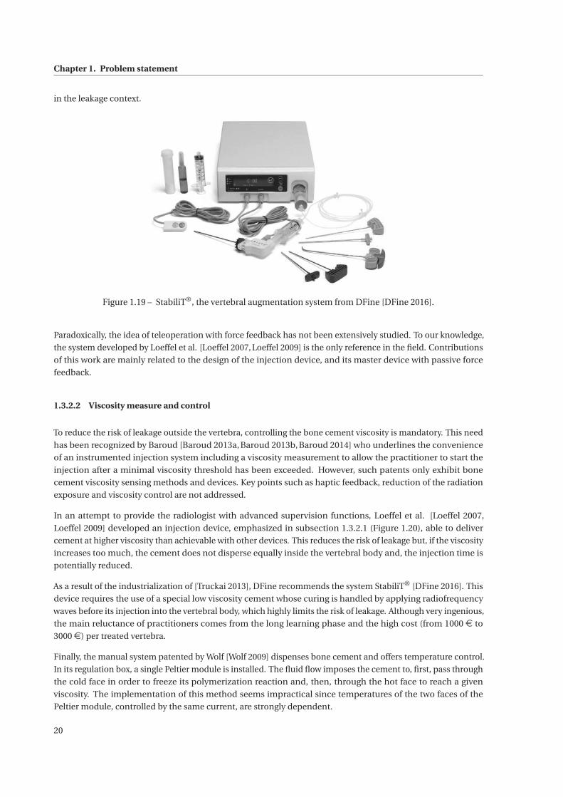
Chapter 1. Problem statement
in the leakage context.
Figure 1.19 – StabiliT®, the vertebral augmentation system from DFine [DFine 2016].
Paradoxically, the idea of teleoperation with force feedback has not been extensively studied. To our knowledge,
the system developed by Loeffel et al. [Loeffel 2007, Loeffel 2009] is the only reference in the field. Contributions
of this work are mainly related to the design of the injection device, and its master device with passive force
feedback.
1.3.2.2 Viscosity measure and control
To reduce the risk of leakage outside the vertebra, controlling the bone cement viscosity is mandatory. This need
has been recognized by Baroud [Baroud 2013a, Baroud 2013b, Baroud 2014] who underlines the convenience
of an instrumented injection system including a viscosity measurement to allow the practitioner to start the
injection after a minimal viscosity threshold has been exceeded. However, such patents only exhibit bone
cement viscosity sensing methods and devices. Key points such as haptic feedback, reduction of the radiation
exposure and viscosity control are not addressed.
In an attempt to provide the radiologist with advanced supervision functions, Loeffel et al. [Loeffel 2007,
Loeffel 2009] developed an injection device, emphasized in subsection 1.3.2.1 (Figure 1.20), able to deliver
cement at higher viscosity than achievable with other devices. This reduces the risk of leakage but, if the viscosity
increases too much, the cement does not disperse equally inside the vertebral body and, the injection time is
potentially reduced.
As a result of the industrialization of [Truckai 2013], DFine recommends the system StabiliT® [DFine 2016]. This
device requires the use of a special low viscosity cement whose curing is handled by applying radiofrequency
waves before its injection into the vertebral body, which highly limits the risk of leakage. Although very ingenious,
the main reluctance of practitioners comes from the long learning phase and the high cost (from 1000 e to
3000e) per treated vertebra.
Finally, the manual system patented by Wolf [Wolf 2009] dispenses bone cement and offers temperature control.
In its regulation box, a single Peltier module is installed. The fluid flow imposes the cement to, first, pass through
the cold face in order to freeze its polymerization reaction and, then, through the hot face to reach a given
viscosity. The implementation of this method seems impractical since temperatures of the two faces of the
Peltier module, controlled by the same current, are strongly dependent.
20
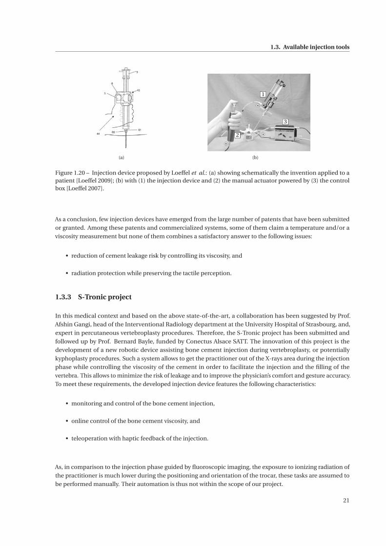
1.3. Available injection tools
(a)
1
3
2
(b)
Figure 1.20 – Injection device proposed by Loeffel et al.: (a) showing schematically the invention applied to apatient [Loeffel 2009]; (b) with (1) the injection device and (2) the manual actuator powered by (3) the controlbox [Loeffel 2007].
As a conclusion, few injection devices have emerged from the large number of patents that have been submitted
or granted. Among these patents and commercialized systems, some of them claim a temperature and/or a
viscosity measurement but none of them combines a satisfactory answer to the following issues:
• reduction of cement leakage risk by controlling its viscosity, and
• radiation protection while preserving the tactile perception.
1.3.3 S-Tronic project
In this medical context and based on the above state-of-the-art, a collaboration has been suggested by Prof.
Afshin Gangi, head of the Interventional Radiology department at the University Hospital of Strasbourg, and,
expert in percutaneous vertebroplasty procedures. Therefore, the S-Tronic project has been submitted and
followed up by Prof. Bernard Bayle, funded by Conectus Alsace SATT. The innovation of this project is the
development of a new robotic device assisting bone cement injection during vertebroplasty, or potentially
kyphoplasty procedures. Such a system allows to get the practitioner out of the X-rays area during the injection
phase while controlling the viscosity of the cement in order to facilitate the injection and the filling of the
vertebra. This allows to minimize the risk of leakage and to improve the physician’s comfort and gesture accuracy.
To meet these requirements, the developed injection device features the following characteristics:
• monitoring and control of the bone cement injection,
• online control of the bone cement viscosity, and
• teleoperation with haptic feedback of the injection.
As, in comparison to the injection phase guided by fluoroscopic imaging, the exposure to ionizing radiation of
the practitioner is much lower during the positioning and orientation of the trocar, these tasks are assumed to
be performed manually. Their automation is thus not within the scope of our project.
21
Chapter 1. Problem statement
1.4 Thesis contributions and organization
1.4.1 Thesis contributions
The objectives of this thesis differ slightly from those of the project. The first aim of this work was to study the
characteristics of the bone cement and to model its behavior in order to determine possible viscosity control
parameters, to dimension the injection device and to determine the appropriate instrumentation to measure
the bone cement viscosity online. Therefore, a rheological study has been set up to help qualify and quantify
parameters influencing the bone cement viscosity. Following the characterization of the bone cement behavior,
the next task was to provide quantitative elements required for the design of the new teleoperated injection
device with force feedback. Based on this study, a first prototype has concurrently been designed by an engineer
from the S-Tronic team. The best control strategy of this device has also been examined. Finally, to control the
evolution of bone cement viscosity, an effort has been required to implement a closed-loop temperature control
providing adapted performances.
1.4.2 Thesis organization
After a short introduction to rheology, chapter 2 presents a rheological study that has been set up to understand
and characterize the behavior of the bone cement viscosity during its polymerization phase.
In Chapter 3, this study results in the identification of two models: a well-known rheological model that has been
improved by adding a temperature dependency and a new original viscosity model, expressed as a nonlinear
differential equation that is exploitable for control purposes.
Chapter 4 develops and justifies the design of a mechatronic injection device in addition to a master interface that
is imperative for the remote control. An analysis of the required online measurements leads to the appropriate
instrumentation of the device. The system dedicated to the control of the flowing bone cement temperature,
validated beforehand by simulations, is also described. Finally, the contradictory properties of the injection
show that, in terms of teleoperation with force feedback, the implementation of the rate control strategy is best
suited.
To control the online viscosity, our solution focuses on the regulation of bone cement temperature. In Chapter 5,
the thermal system has been modeled and identified by considering the flowing bone cement and the emitted
heat flux. This allows us to propose a satisfactory temperature control and, thus, viscosity control.
The injection device and its benefits are discussed in the conclusion, along with the prospects of this work.
Improvements of the injection device are suggested at different levels.
22
2 Rheology of bone cement
Contents
2.1 Aspects of rheology . . . . . . . . . . . . . . . . . . . . . . . . . . . . . . . . . . . . . . . . . . . . . . . 24
2.1.1 Definitions . . . . . . . . . . . . . . . . . . . . . . . . . . . . . . . . . . . . . . . . . . . . . . . . 24
2.1.2 Rheological behaviors . . . . . . . . . . . . . . . . . . . . . . . . . . . . . . . . . . . . . . . . . 25
2.1.3 Rheometers . . . . . . . . . . . . . . . . . . . . . . . . . . . . . . . . . . . . . . . . . . . . . . . 26
2.2 Acrylic bone cement . . . . . . . . . . . . . . . . . . . . . . . . . . . . . . . . . . . . . . . . . . . . . . 29
2.2.1 Chemical aspect . . . . . . . . . . . . . . . . . . . . . . . . . . . . . . . . . . . . . . . . . . . . 29
2.2.2 Bone cement rheological properties . . . . . . . . . . . . . . . . . . . . . . . . . . . . . . . . . 30
2.2.3 Viscosity modeling . . . . . . . . . . . . . . . . . . . . . . . . . . . . . . . . . . . . . . . . . . . 31
2.3 Rheological study . . . . . . . . . . . . . . . . . . . . . . . . . . . . . . . . . . . . . . . . . . . . . . . . 34
2.3.1 Viscosity measurement . . . . . . . . . . . . . . . . . . . . . . . . . . . . . . . . . . . . . . . . 34
2.3.2 Experiments . . . . . . . . . . . . . . . . . . . . . . . . . . . . . . . . . . . . . . . . . . . . . . . 36
2.3.3 Analysis . . . . . . . . . . . . . . . . . . . . . . . . . . . . . . . . . . . . . . . . . . . . . . . . . 38
23
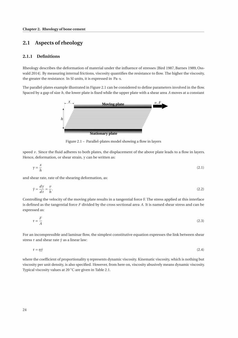
Chapter 2. Rheology of bone cement
2.1 Aspects of rheology
2.1.1 Definitions
Rheology describes the deformation of material under the influence of stresses [Bird 1987, Barnes 1989, Oss-
wald 2014]. By measuring internal frictions, viscosity quantifies the resistance to flow. The higher the viscosity,
the greater the resistance. In SI units, it is expressed in Pa·s.
The parallel-plates example illustrated in Figure 2.1 can be considered to define parameters involved in the flow.
Spaced by a gap of size h, the lower plate is fixed while the upper plate with a shear area A moves at a constant
h
x v , F
Stationary plate
Moving plate
Figure 2.1 – Parallel-plates model showing a flow in layers
speed v . Since the fluid adheres to both plates, the displacement of the above plate leads to a flow in layers.
Hence, deformation, or shear strain, γ can be written as:
γ= x
h(2.1)
and shear rate, rate of the shearing deformation, as:
γ= dγ
d t= v
h. (2.2)
Controlling the velocity of the moving plate results in a tangential force F. The stress applied at this interface
is defined as the tangential force F divided by the cross sectional area A. It is named shear stress and can be
expressed as:
τ= F
A(2.3)
For an incompressible and laminar flow, the simplest constitutive equation expresses the link between shear
stress τ and shear rate γ as a linear law:
τ= ηγ (2.4)
where the coefficient of proportionality η represents dynamic viscosity. Kinematic viscosity, which is nothing but
viscosity per unit density, is also specified. However, from here on, viscosity abusively means dynamic viscosity.
Typical viscosity values at 20 ◦C are given in Table 2.1.
24
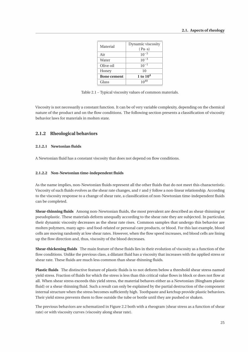
2.1. Aspects of rheology
MaterialDynamic viscosity
( Pa·s)
Air 10−5
Water 10−3
Olive oil 10−1
Honey 10
Bone cement 1 to 104
Glass 1040
Table 2.1 – Typical viscosity values of common materials.
Viscosity is not necessarily a constant function. It can be of very variable complexity, depending on the chemical
nature of the product and on the flow conditions. The following section presents a classification of viscosity
behavior laws for materials in molten state.
2.1.2 Rheological behaviors
2.1.2.1 Newtonian fluids
A Newtonian fluid has a constant viscosity that does not depend on flow conditions.
2.1.2.2 Non-Newtonian time-independent fluids
As the name implies, non-Newtonian fluids represent all the other fluids that do not meet this characteristic.
Viscosity of such fluids evolves as the shear rate changes, and τ and γ follow a non-linear relationship. According
to the viscosity response to a change of shear rate, a classification of non-Newtonian time-independent fluids
can be completed.
Shear-thinning fluids Among non-Newtonian fluids, the most prevalent are described as shear-thinning or
pseudoplastic. These materials deform unequally according to the shear rate they are subjected. In particular,
their dynamic viscosity decreases as the shear rate rises. Common samples that undergo this behavior are
molten polymers, many agro- and food-related or personal care products, or blood. For this last example, blood
cells are moving randomly at low shear rates. However, when the flow speed increases, red blood cells are lining
up the flow direction and, thus, viscosity of the blood decreases.
Shear-thickening fluids The main feature of these fluids lies in their evolution of viscosity as a function of the
flow conditions. Unlike the previous class, a dilatant fluid has a viscosity that increases with the applied stress or
shear rate. These fluids are much less common than shear-thinning fluids.
Plastic fluids The distinctive feature of plastic fluids is to not deform below a threshold shear stress named
yield stress. Fraction of fluids for which the stress is less than this critical value flows in block or does not flow at
all. When shear stress exceeds this yield stress, the material behaves either as a Newtonian (Bingham plastic
fluid) or a shear-thinning fluid. Such a result can only be explained by the partial destruction of the component
internal structure when the stress becomes sufficiently high. Toothpaste and ketchup provide plastic behaviors.
Their yield stress prevents them to flow outside the tube or bottle until they are pushed or shaken.
The previous behaviors are schematized in Figure 2.2 both with a rheogram (shear stress as a function of shear
rate) or with viscosity curves (viscosity along shear rate).
25
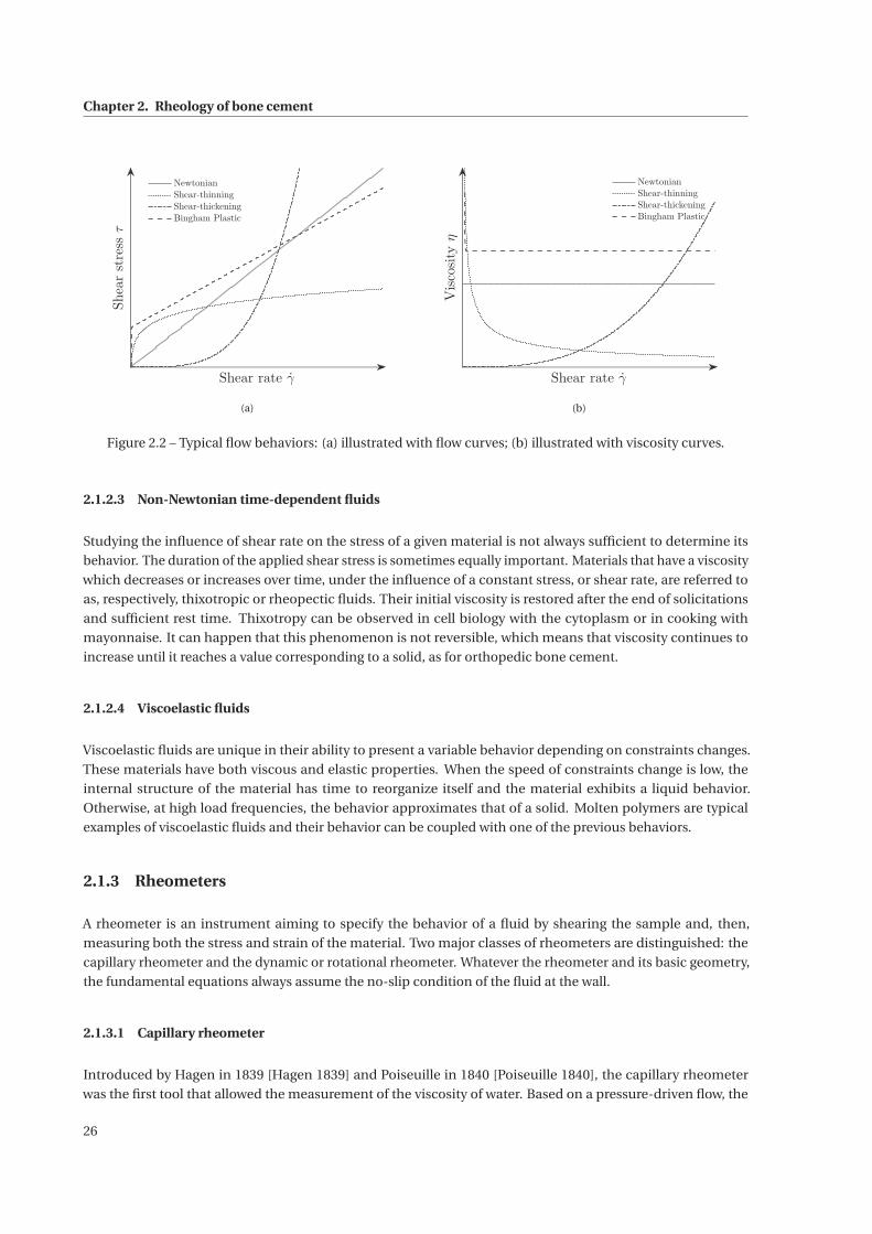
Chapter 2. Rheology of bone cement
Shear rate γ
Shearstressτ
Newtonian
Shear-thinning
Shear-thickening
Bingham Plastic
(a)
Shear rate γ
Viscosityη
Newtonian
Shear-thinning
Shear-thickening
Bingham Plastic
(b)
Figure 2.2 – Typical flow behaviors: (a) illustrated with flow curves; (b) illustrated with viscosity curves.
2.1.2.3 Non-Newtonian time-dependent fluids
Studying the influence of shear rate on the stress of a given material is not always sufficient to determine its
behavior. The duration of the applied shear stress is sometimes equally important. Materials that have a viscosity
which decreases or increases over time, under the influence of a constant stress, or shear rate, are referred to
as, respectively, thixotropic or rheopectic fluids. Their initial viscosity is restored after the end of solicitations
and sufficient rest time. Thixotropy can be observed in cell biology with the cytoplasm or in cooking with
mayonnaise. It can happen that this phenomenon is not reversible, which means that viscosity continues to
increase until it reaches a value corresponding to a solid, as for orthopedic bone cement.
2.1.2.4 Viscoelastic fluids
Viscoelastic fluids are unique in their ability to present a variable behavior depending on constraints changes.
These materials have both viscous and elastic properties. When the speed of constraints change is low, the
internal structure of the material has time to reorganize itself and the material exhibits a liquid behavior.
Otherwise, at high load frequencies, the behavior approximates that of a solid. Molten polymers are typical
examples of viscoelastic fluids and their behavior can be coupled with one of the previous behaviors.
2.1.3 Rheometers
A rheometer is an instrument aiming to specify the behavior of a fluid by shearing the sample and, then,
measuring both the stress and strain of the material. Two major classes of rheometers are distinguished: the
capillary rheometer and the dynamic or rotational rheometer. Whatever the rheometer and its basic geometry,
the fundamental equations always assume the no-slip condition of the fluid at the wall.
2.1.3.1 Capillary rheometer
Introduced by Hagen in 1839 [Hagen 1839] and Poiseuille in 1840 [Poiseuille 1840], the capillary rheometer
was the first tool that allowed the measurement of the viscosity of water. Based on a pressure-driven flow, the
26
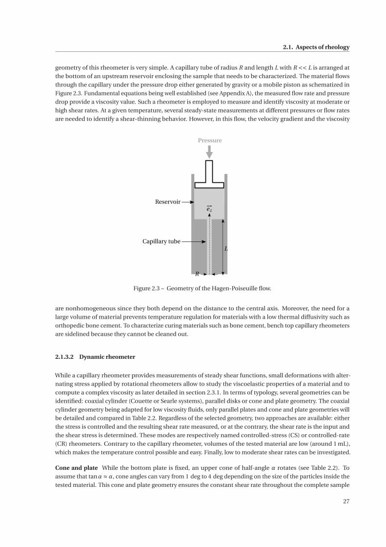
2.1. Aspects of rheology
geometry of this rheometer is very simple. A capillary tube of radius R and length L with R << L is arranged at
the bottom of an upstream reservoir enclosing the sample that needs to be characterized. The material flows
through the capillary under the pressure drop either generated by gravity or a mobile piston as schematized in
Figure 2.3. Fundamental equations being well established (see Appendix A), the measured flow rate and pressure
drop provide a viscosity value. Such a rheometer is employed to measure and identify viscosity at moderate or
high shear rates. At a given temperature, several steady-state measurements at different pressures or flow rates
are needed to identify a shear-thinning behavior. However, in this flow, the velocity gradient and the viscosity
R
L
−→ez
Pressure
Reservoir
Capillary tube
Figure 2.3 – Geometry of the Hagen-Poiseuille flow.
are nonhomogeneous since they both depend on the distance to the central axis. Moreover, the need for a
large volume of material prevents temperature regulation for materials with a low thermal diffusivity such as
orthopedic bone cement. To characterize curing materials such as bone cement, bench top capillary rheometers
are sidelined because they cannot be cleaned out.
2.1.3.2 Dynamic rheometer
While a capillary rheometer provides measurements of steady shear functions, small deformations with alter-
nating stress applied by rotational rheometers allow to study the viscoelastic properties of a material and to
compute a complex viscosity as later detailed in section 2.3.1. In terms of typology, several geometries can be
identified: coaxial cylinder (Couette or Searle systems), parallel disks or cone and plate geometry. The coaxial
cylinder geometry being adapted for low viscosity fluids, only parallel plates and cone and plate geometries will
be detailed and compared in Table 2.2. Regardless of the selected geometry, two approaches are available: either
the stress is controlled and the resulting shear rate measured, or at the contrary, the shear rate is the input and
the shear stress is determined. These modes are respectively named controlled-stress (CS) or controlled-rate
(CR) rheometers. Contrary to the capillary rheometer, volumes of the tested material are low (around 1 mL),
which makes the temperature control possible and easy. Finally, low to moderate shear rates can be investigated.
Cone and plate While the bottom plate is fixed, an upper cone of half-angle α rotates (see Table 2.2). To
assume that tanα≈α, cone angles can vary from 1 deg to 4 deg depending on the size of the particles inside the
tested material. This cone and plate geometry ensures the constant shear rate throughout the complete sample
27
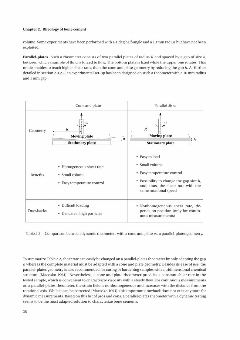
Chapter 2. Rheology of bone cement
volume. Some experiments have been performed with a 4 deg half-angle and a 10 mm radius but have not been
exploited.
Parallel-plates Such a rheometer consists of two parallel plates of radius R and spaced by a gap of size h,
between which a sample of fluid is forced to flow. The bottom plate is fixed while the upper one rotates. This
mode enables to reach higher shear rates than the cone and plate geometry by reducing the gap h. As further
detailed in section 2.3.2.1, an experimental set-up has been designed on such a rheometer with a 10 mm radius
and 1 mm gap.
Cone and plate Parallel disks
Geometry
ω
R
Stationary plate
Moving plateα
R
ω
hStationary plate
Moving plate
Benefits
• Homogeneous shear rate
• Small volume
• Easy temperature control
• Easy to load
• Small volume
• Easy temperature control
• Possibility to change the gap size h,and, thus, the shear rate with thesame rotational speed
Drawbacks
• Difficult loading
• Delicate if high particles
• Nonhomogeneous shear rate, de-pends on position (only for contin-uous measurements)
Table 2.2 – Comparison between dynamic rheometers with a cone and plate vs. a parallel-plates geometry.
To summarize Table 2.2, shear rate can easily be changed on a parallel-plates rheometer by only adapting the gap
h whereas the complete material must be adapted with a cone and plate geometry. Besides its ease of use, the
parallel-plates geometry is also recommended for curing or hardening samples with a tridimensional chemical
structure [Macosko 1994]. Nevertheless, a cone and plate rheometer provides a constant shear rate in the
tested sample, which is convenient to characterize viscosity with a steady flow. For continuous measurements
on a parallel-plates rheometer, the strain field is nonhomogeneous and increases with the distance from the
rotational axis. While it can be corrected [Macosko 1994], this important drawback does not exist anymore for
dynamic measurements. Based on this list of pros and cons, a parallel-plates rheometer with a dynamic testing
seems to be the most adapted solution to characterize bone cements.
28
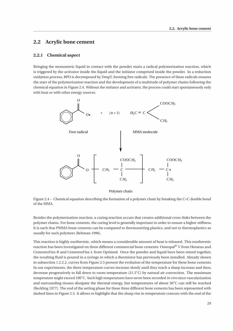
2.2. Acrylic bone cement
2.2 Acrylic bone cement
2.2.1 Chemical aspect
Bringing the monomeric liquid in contact with the powder starts a radical polymerization reaction, which
is triggered by the activator inside the liquid and the initiator comprised inside the powder. In a reduction
oxidation process, BPO is decomposed by DmpT, forming free radicals. The presence of these radicals ensures
the start of the polymerization reaction and the development of a multitude of polymer chains following the
chemical equation in Figure 2.4. Without the initiator and activator, the process could start spontaneously only
with heat or with other energy sources.
(n +1) H2C
COOC H3
C H3
O
C H2 C
COOC H3
C H3
C H2 C
COOC H3
C H3
C
O
O +
Free radical MMA molecule
Polymer chain
O
Figure 2.4 – Chemical equation describing the formation of a polymer chain by breaking the C=C double bondof the MMA.
Besides the polymerization reaction, a curing reaction occurs that creates additional cross-links between the
polymer chains. For bone cements, the curing level is generally important in order to ensure a higher stiffness.
It is such that PMMA bone cements can be compared to thermosetting plastics, and not to thermoplastics as
usually for such polymers [Rehman 1996].
This reaction is highly exothermic, which means a considerable amount of heat is released. This exothermic
reaction has been investigated on three different commercial bone cements: Osteopal® V from Heraeus and
CementoFixx-R and CementoFixx-L from Optimed. Once the powder and liquid have been mixed together,
the resulting fluid is poured in a syringe in which a thermistor has previously been installed. Already shown
in subsection 1.2.2.2, curves from Figure 2.5 present the evolution of the temperature for these bone cements.
In our experiments, the three temperature curves increase slowly until they reach a sharp increase and then,
decrease progressively to fall down to room temperature (21.5◦C) by natural air convection. The maximum
temperature might exceed 100◦C. Such high temperatures have never been recorded in vivo since vascularization
and surrounding tissues dissipate the thermal energy, but temperatures of about 50◦C can still be reached
[Reckling 1977]. The end of the setting phase for these three different bone cements has been represented with
dashed lines in Figure 2.5. It allows to highlight that the sharp rise in temperature concurs with the end of the
29
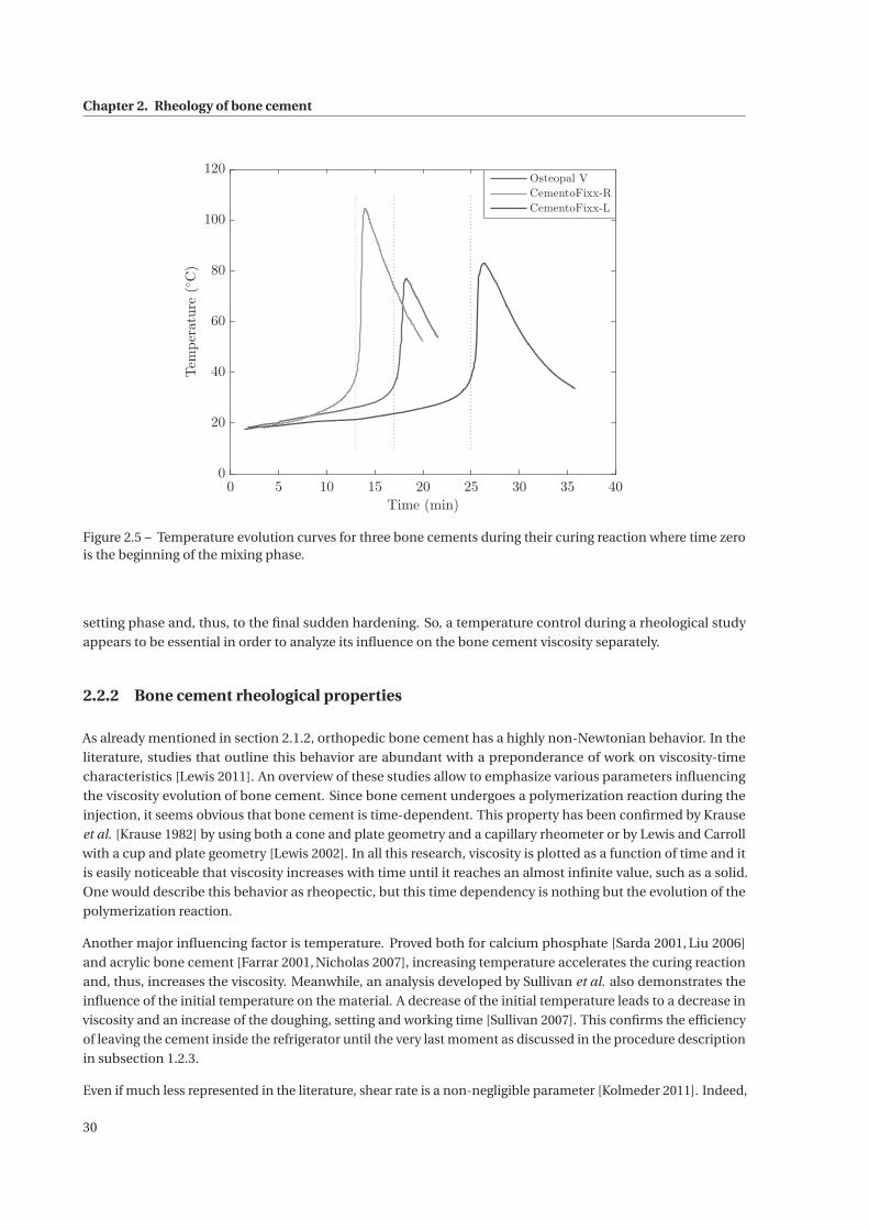
Chapter 2. Rheology of bone cement
0 5 10 15 20 25 30 35 40
Time (min)
0
20
40
60
80
100
120
Temperature(◦C)
Osteopal V
CementoFixx-R
CementoFixx-L
Figure 2.5 – Temperature evolution curves for three bone cements during their curing reaction where time zerois the beginning of the mixing phase.
setting phase and, thus, to the final sudden hardening. So, a temperature control during a rheological study
appears to be essential in order to analyze its influence on the bone cement viscosity separately.
2.2.2 Bone cement rheological properties
As already mentioned in section 2.1.2, orthopedic bone cement has a highly non-Newtonian behavior. In the
literature, studies that outline this behavior are abundant with a preponderance of work on viscosity-time
characteristics [Lewis 2011]. An overview of these studies allow to emphasize various parameters influencing
the viscosity evolution of bone cement. Since bone cement undergoes a polymerization reaction during the
injection, it seems obvious that bone cement is time-dependent. This property has been confirmed by Krause
et al. [Krause 1982] by using both a cone and plate geometry and a capillary rheometer or by Lewis and Carroll
with a cup and plate geometry [Lewis 2002]. In all this research, viscosity is plotted as a function of time and it
is easily noticeable that viscosity increases with time until it reaches an almost infinite value, such as a solid.
One would describe this behavior as rheopectic, but this time dependency is nothing but the evolution of the
polymerization reaction.
Another major influencing factor is temperature. Proved both for calcium phosphate [Sarda 2001, Liu 2006]
and acrylic bone cement [Farrar 2001, Nicholas 2007], increasing temperature accelerates the curing reaction
and, thus, increases the viscosity. Meanwhile, an analysis developed by Sullivan et al. also demonstrates the
influence of the initial temperature on the material. A decrease of the initial temperature leads to a decrease in
viscosity and an increase of the doughing, setting and working time [Sullivan 2007]. This confirms the efficiency
of leaving the cement inside the refrigerator until the very last moment as discussed in the procedure description
in subsection 1.2.3.
Even if much less represented in the literature, shear rate is a non-negligible parameter [Kolmeder 2011]. Indeed,
30
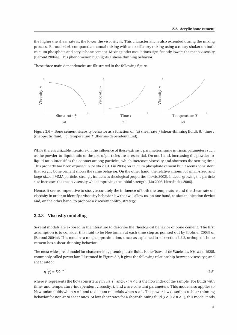
2.2. Acrylic bone cement
the higher the shear rate is, the lower the viscosity is. This characteristic is also extended during the mixing
process. Baroud et al. compared a manual mixing with an oscillatory mixing using a rotary shaker on both
calcium phosphate and acrylic bone cement. Mixing under oscillations significantly lowers the mean viscosity
[Baroud 2004a]. This phenomenon highlights a shear-thinning behavior.
These three main dependencies are illustrated in the following figure.
Shear rate γ
Viscosityη
(a)
Time t
Viscosityη
(b)
Temperature T
Viscosityη
(c)
Figure 2.6 – Bone cement viscosity behavior as a function of: (a) shear rate γ (shear-thinning fluid); (b) time t(rheopectic fluid); (c) temperature T (thermo-dependent fluid).
While there is a sizable literature on the influence of these extrinsic parameters, some intrinsic parameters such
as the powder-to-liquid ratio or the size of particles are as essential. On one hand, increasing the powder-to-
liquid ratio intensifies the contact among particles, which increases viscosity and shortens the setting time.
This property has been exposed in [Sarda 2001, Liu 2006] on calcium phosphate cement but it seems consistent
that acrylic bone cement shows the same behavior. On the other hand, the relative amount of small-sized and
large-sized PMMA particles strongly influences rheological properties [Lewis 2002]. Indeed, growing the particle
size increases the mean viscosity while improving the initial strength [Liu 2006, Hernández 2006].
Hence, it seems imperative to study accurately the influence of both the temperature and the shear rate on
viscosity in order to identify a viscosity behavior law that will allow us, on one hand, to size an injection device
and, on the other hand, to propose a viscosity control strategy.
2.2.3 Viscosity modeling
Several models are exposed in the literature to describe the rheological behavior of bone cement. The first
assumption is to consider this fluid to be Newtonian at each time step as pointed out by [Bohner 2003] or
[Baroud 2004a]. This remains a rough approximation, since, as explained in subsection 2.2.2, orthopedic bone
cement has a shear-thinning behavior.
The most widespread model for characterizing pseudoplastic fluids is the Ostwald-de Waele law [Ostwald 1925],
commonly called power law. Illustrated in Figure 2.7, it gives the following relationship between viscosity η and
shear rate γ:
η(γ)= K γn−1 (2.5)
where K represents the flow consistency in Pa·sn and 0 < n < 1 is the flow index of the sample. For fluids with
time- and temperature-independent viscosity, K and n are constant parameters. This model also applies to
Newtonian fluids when n = 1 and to dilatant materials when n > 1. The power law describes a shear-thinning
behavior for non-zero shear rates. At low shear rates for a shear-thinning fluid (i.e. 0 < n < 1), this model tends
31
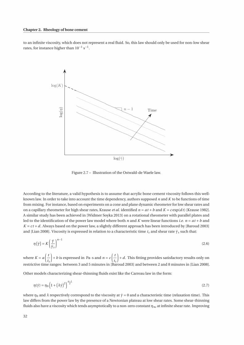
Chapter 2. Rheology of bone cement
to an infinite viscosity, which does not represent a real fluid. So, this law should only be used for non-low shear
rates, for instance higher than 10−1 s−1.
log(γ)
log(η)
log(K)
n− 1 Time
Figure 2.7 – Illustration of the Ostwald-de Waele law.
According to the literature, a valid hypothesis is to assume that acrylic bone cement viscosity follows this well-
known law. In order to take into account the time dependency, authors supposed n and K to be functions of time
from mixing. For instance, based on experiments on a cone and plane dynamic rheometer for low shear rates and
on a capillary rheometer for high shear rates, Krause et al. identified n = at +b and K = c exp(d t ) [Krause 1982].
A similar study has been achieved in [Widmer Soyka 2013] on a rotational rheometer with parallel plates and
led to the identification of the power law model where both n and K were linear functions i.e. n = at +b and
K = ct +d . Always based on the power law, a slightly different approach has been introduced by [Baroud 2003]
and [Lian 2008]. Viscosity is expressed in relation to a characteristic time ts and shear rate γs such that:
η(γ)= K
(γ
γs
)n−1
(2.6)
where K = a
(t
ts
)+b is expressed in Pa·s and n = c
(t
ts
)+d . This fitting provides satisfactory results only on
restrictive time ranges: between 3 and 5 minutes in [Baroud 2003] and between 2 and 8 minutes in [Lian 2008].
Other models characterizing shear-thinning fluids exist like the Carreau law in the form:
η(γ) = η0
(1+
(λγ
)2) n−1
2(2.7)
where η0 and λ respectively correspond to the viscosity at γ= 0 and a characteristic time (relaxation time). This
law differs from the power law by the presence of a Newtonian plateau at low shear rates. Some shear-thinning
fluids also have a viscosity which tends asymptotically to a non-zero constant η∞ at infinite shear rate. Improving
32
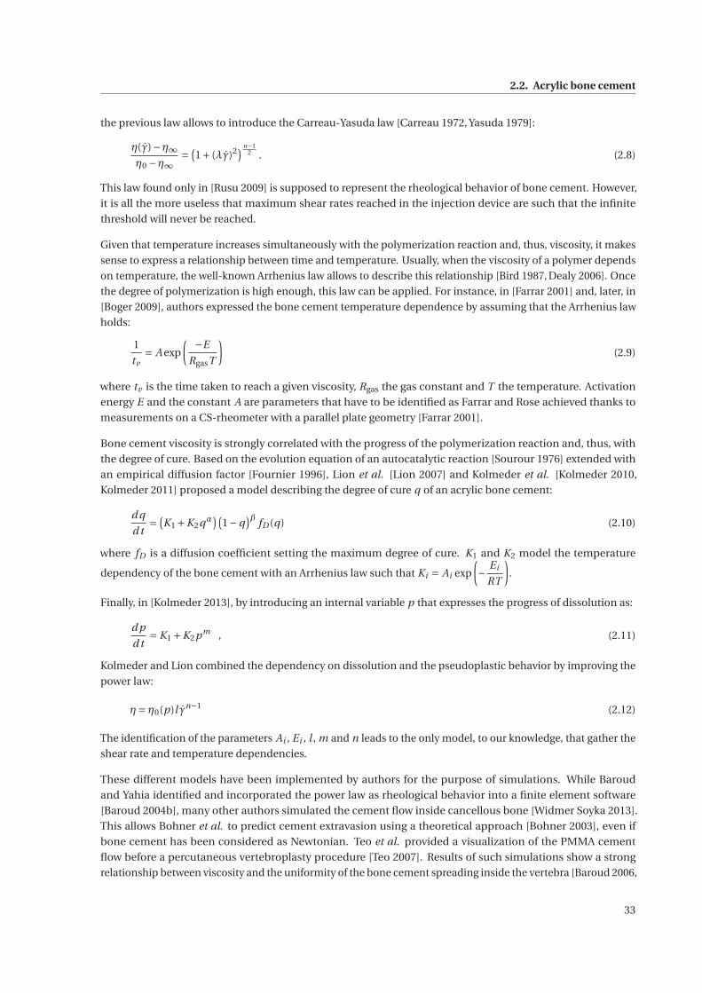
2.2. Acrylic bone cement
the previous law allows to introduce the Carreau-Yasuda law [Carreau 1972, Yasuda 1979]:
η(γ)−η∞η0 −η∞
=(1+ (λγ)2) n−1
2 . (2.8)
This law found only in [Rusu 2009] is supposed to represent the rheological behavior of bone cement. However,
it is all the more useless that maximum shear rates reached in the injection device are such that the infinite
threshold will never be reached.
Given that temperature increases simultaneously with the polymerization reaction and, thus, viscosity, it makes
sense to express a relationship between time and temperature. Usually, when the viscosity of a polymer depends
on temperature, the well-known Arrhenius law allows to describe this relationship [Bird 1987, Dealy 2006]. Once
the degree of polymerization is high enough, this law can be applied. For instance, in [Farrar 2001] and, later, in
[Boger 2009], authors expressed the bone cement temperature dependence by assuming that the Arrhenius law
holds:
1
tv= A exp
( −E
RgasT
)(2.9)
where tv is the time taken to reach a given viscosity, Rgas the gas constant and T the temperature. Activation
energy E and the constant A are parameters that have to be identified as Farrar and Rose achieved thanks to
measurements on a CS-rheometer with a parallel plate geometry [Farrar 2001].
Bone cement viscosity is strongly correlated with the progress of the polymerization reaction and, thus, with
the degree of cure. Based on the evolution equation of an autocatalytic reaction [Sourour 1976] extended with
an empirical diffusion factor [Fournier 1996], Lion et al. [Lion 2007] and Kolmeder et al. [Kolmeder 2010,
Kolmeder 2011] proposed a model describing the degree of cure q of an acrylic bone cement:
d q
d t=(K1 +K2qα
)(1−q
)β fD (q) (2.10)
where fD is a diffusion coefficient setting the maximum degree of cure. K1 and K2 model the temperature
dependency of the bone cement with an Arrhenius law such that Ki = Ai exp
(− Ei
RT
).
Finally, in [Kolmeder 2013], by introducing an internal variable p that expresses the progress of dissolution as:
d p
d t= K1 +K2pm , (2.11)
Kolmeder and Lion combined the dependency on dissolution and the pseudoplastic behavior by improving the
power law:
η= η0(p)l γn−1 (2.12)
The identification of the parameters Ai , Ei , l , m and n leads to the only model, to our knowledge, that gather the
shear rate and temperature dependencies.
These different models have been implemented by authors for the purpose of simulations. While Baroud
and Yahia identified and incorporated the power law as rheological behavior into a finite element software
[Baroud 2004b], many other authors simulated the cement flow inside cancellous bone [Widmer Soyka 2013].
This allows Bohner et al. to predict cement extravasion using a theoretical approach [Bohner 2003], even if
bone cement has been considered as Newtonian. Teo et al. provided a visualization of the PMMA cement
flow before a percutaneous vertebroplasty procedure [Teo 2007]. Results of such simulations show a strong
relationship between viscosity and the uniformity of the bone cement spreading inside the vertebra [Baroud 2006,
33
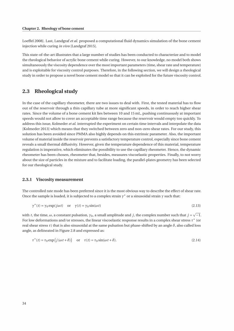
Chapter 2. Rheology of bone cement
Loeffel 2008]. Last, Landgraf et al. proposed a computational fluid dynamics simulation of the bone cement
injection while curing in vivo [Landgraf 2015].
This state-of-the-art illustrates that a large number of studies has been conducted to characterize and to model
the rheological behavior of acrylic bone cement while curing. However, to our knowledge, no model both shows
simultaneously the viscosity dependence over the most important parameters (time, shear rate and temperature)
and is exploitable for viscosity control purposes. Therefore, in the following section, we will design a rheological
study in order to propose a novel bone cement model so that it can be exploited for the future viscosity control.
2.3 Rheological study
In the case of the capillary rheometer, there are two issues to deal with. First, the tested material has to flow
out of the reservoir through a thin capillary tube at more significant speeds, in order to reach higher shear
rates. Since the volume of a bone cement kit lies between 10 and 15 mL, pushing continuously at important
speeds would not allow to cover an acceptable time range because the reservoir would empty too quickly. To
address this issue, Kolmeder et al. interrupted the experiment on certain time intervals and interpolate the data
[Kolmeder 2013] which means that they switched between zero and non-zero shear rates. For our study, this
solution has been avoided since PMMA also highly depends on this extrinsic parameter. Also, the important
volume of material inside the reservoir prevents a satisfactory temperature control, especially since bone cement
reveals a small thermal diffusivity. However, given the temperature dependence of this material, temperature
regulation is imperative, which eliminates the possibility to use the capillary rheometer. Hence, the dynamic
rheometer has been chosen, rheometer that, besides, measures viscoelastic properties. Finally, to not worry
about the size of particles in the mixture and to facilitate loading, the parallel-plates geometry has been selected
for our rheological study.
2.3.1 Viscosity measurement
The controlled rate mode has been preferred since it is the most obvious way to describe the effect of shear rate.
Once the sample is loaded, it is subjected to a complex strain γ∗ or a sinusoidal strain γ such that:
γ∗(t ) = γ0 exp( jωt ) or γ(t ) = γ0 sin(ωt ) (2.13)
with t , the time, ω, a constant pulsation, γ0, a small amplitude and j , the complex number such that j =−1.
For low deformations and/or stresses, the linear viscoelastic response results in a complex shear stress τ∗ (or
real shear stress τ) that is also sinusoidal at the same pulsation but phase-shifted by an angle δ, also called loss
angle, as delineated in Figure 2.8 and expressed as:
τ∗(t ) = τ0 exp(
j (ωt +δ))
or τ(t ) = τ0 sin(ωt +δ). (2.14)
34
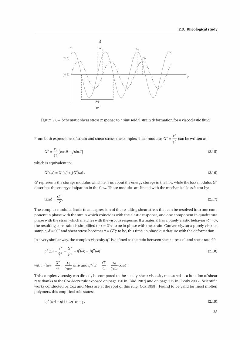
2.3. Rheological study
tγ(t )
τ(t )
δ
ω τ0
γ0
2π
ω
Figure 2.8 – Schematic shear stress response to a sinusoidal strain deformation for a viscoelastic fluid.
From both expressions of strain and shear stress, the complex shear modulus G∗ = τ∗
γ∗can be written as:
G∗ = τ0
γ0
(cosδ+ j sinδ
)(2.15)
which is equivalent to:
G∗(ω) =G ′(ω)+ jG ′′(ω) . (2.16)
G ′ represents the storage modulus which tells us about the energy storage in the flow while the loss modulus G ′′
describes the energy dissipation in the flow. These modules are linked with the mechanical loss factor by:
tanδ= G ′′
G ′ . (2.17)
The complex modulus leads to an expression of the resulting shear stress that can be resolved into one com-
ponent in phase with the strain which coincides with the elastic response, and one component in quadrature
phase with the strain which matches with the viscous response. If a material has a purely elastic behavior (δ= 0),
the resulting constraint is simplified to τ=G ′γ to be in phase with the strain. Conversely, for a purely viscous
sample, δ= 90◦ and shear stress becomes τ=G ′′γ to be, this time, in phase quadrature with the deformation.
In a very similar way, the complex viscosity η∗ is defined as the ratio between shear stress τ∗ and shear rate γ∗:
η∗(ω) = τ∗
γ∗= G∗
jω= η′(ω)− jη′′(ω) (2.18)
with η′(ω) = G ′′
ω= τ0
γ0ωsinδ and η′′(ω) = G ′
ω= τ0
γ0ωcosδ.
This complex viscosity can directly be compared to the steady-shear viscosity measured as a function of shear
rate thanks to the Cox-Merz rule exposed on page 150 in [Bird 1987] and on page 375 in [Dealy 2006]. Scientific
works conducted by Cox and Merz are at the root of this rule [Cox 1958]. Found to be valid for most molten
polymers, this empirical rule states:
|η∗(ω)| = η(γ) for ω= γ. (2.19)
35
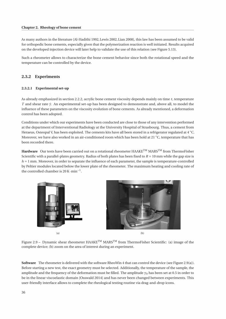
Chapter 2. Rheology of bone cement
As many authors in the literature [Al-Hadithi 1992, Lewis 2002, Lian 2008], this law has been assumed to be valid
for orthopedic bone cements, especially given that the polymerization reaction is well initiated. Results acquired
on the developed injection device will later help to validate the use of this relation (see Figure 5.13).
Such a rheometer allows to characterize the bone cement behavior since both the rotational speed and the
temperature can be controlled by the device.
2.3.2 Experiments
2.3.2.1 Experimental set-up
As already emphasized in section 2.2.2, acrylic bone cement viscosity depends mainly on time t , temperature
T and shear rate γ. An experimental set-up has been designed to demonstrate and, above all, to model the
influence of these parameters on the viscosity evolution of bone cements. As already mentioned, a deformation
control has been adopted.
Conditions under which our experiments have been conducted are close to those of any intervention performed
at the department of Interventional Radiology at the University Hospital of Strasbourg. Thus, a cement from
Heraeus, Osteopal V, has been exploited. The cements kits have all been stored in a refrigerator regulated at 4 ◦C.
Moreover, we have also worked in an air-conditioned room which has been hold at 21 ◦C, temperature that has
been recorded there.
Hardware Our tests have been carried out on a rotational rheometer HAAKETM MARSTM from ThermoFisher
Scientific with a parallel-plates geometry. Radius of both plates has been fixed to R = 10 mm while the gap size is
h = 1 mm. Moreover, in order to separate the influence of each parameter, the sample is temperature-controlled
by Peltier modules located below the lower plate of the rheometer. The maximum heating and cooling rate of
the controlled chamber is 20 K·min−1.
(a) (b)
Figure 2.9 – Dynamic shear rheometer HAAKETM MARSTM from ThermoFisher Scientific: (a) image of thecomplete device; (b) zoom on the area of interest during an experiment.
Software The rheometer is delivered with the software RheoWin 4 that can control the device (see Figure 2.9(a)).
Before starting a new test, the exact geometry must be selected. Additionally, the temperature of the sample, the
amplitude and the frequency of the deformation must be filled. The amplitude γ0 has been set at 0.5 in order to
be in the linear viscoelastic domain [Osswald 2014] and has never been changed between experiments. This
user-friendly interface allows to complete the rheological testing routine via drag-and-drop icons.
36
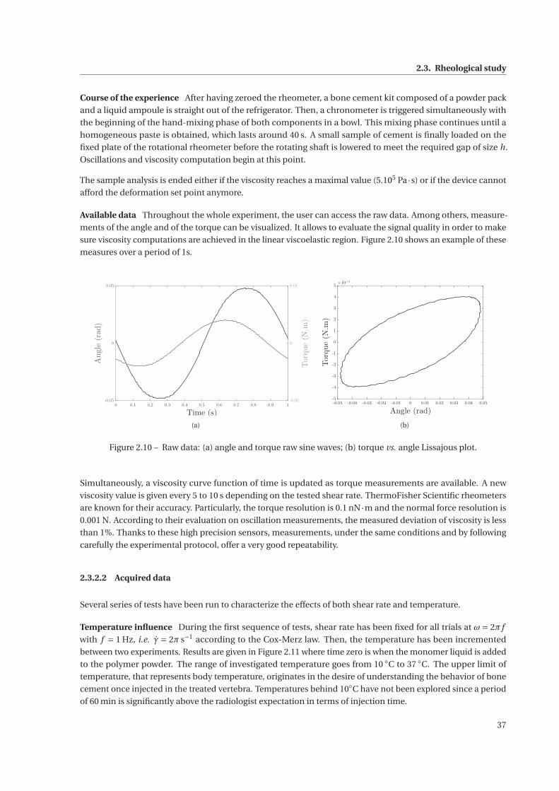
2.3. Rheological study
Course of the experience After having zeroed the rheometer, a bone cement kit composed of a powder pack
and a liquid ampoule is straight out of the refrigerator. Then, a chronometer is triggered simultaneously with
the beginning of the hand-mixing phase of both components in a bowl. This mixing phase continues until a
homogeneous paste is obtained, which lasts around 40 s. A small sample of cement is finally loaded on the
fixed plate of the rotational rheometer before the rotating shaft is lowered to meet the required gap of size h.
Oscillations and viscosity computation begin at this point.
The sample analysis is ended either if the viscosity reaches a maximal value (5.105 Pa·s) or if the device cannot
afford the deformation set point anymore.
Available data Throughout the whole experiment, the user can access the raw data. Among others, measure-
ments of the angle and of the torque can be visualized. It allows to evaluate the signal quality in order to make
sure viscosity computations are achieved in the linear viscoelastic region. Figure 2.10 shows an example of these
measures over a period of 1s.
0 0.1 0.2 0.3 0.4 0.5 0.6 0.7 0.8 0.9 1
Time (s)
-0.05
0
0.05
Angle
(rad)
-0.01
0
0.01
Torque(N.m
)
(a)
-0.05 -0.04 -0.03 -0.02 -0.01 0 0.01 0.02 0.03 0.04 0.05
Angle (rad)
-5
-4
-3
-2
-1
0
1
2
3
4
5
Torque(N.m
)
×10−3
(b)
Figure 2.10 – Raw data: (a) angle and torque raw sine waves; (b) torque vs. angle Lissajous plot.
Simultaneously, a viscosity curve function of time is updated as torque measurements are available. A new
viscosity value is given every 5 to 10 s depending on the tested shear rate. ThermoFisher Scientific rheometers
are known for their accuracy. Particularly, the torque resolution is 0.1 nN·m and the normal force resolution is
0.001 N. According to their evaluation on oscillation measurements, the measured deviation of viscosity is less
than 1%. Thanks to these high precision sensors, measurements, under the same conditions and by following
carefully the experimental protocol, offer a very good repeatability.
2.3.2.2 Acquired data
Several series of tests have been run to characterize the effects of both shear rate and temperature.
Temperature influence During the first sequence of tests, shear rate has been fixed for all trials at ω = 2π f
with f = 1 Hz, i.e. γ = 2π s−1 according to the Cox-Merz law. Then, the temperature has been incremented
between two experiments. Results are given in Figure 2.11 where time zero is when the monomer liquid is added
to the polymer powder. The range of investigated temperature goes from 10 ◦C to 37 ◦C. The upper limit of
temperature, that represents body temperature, originates in the desire of understanding the behavior of bone
cement once injected in the treated vertebra. Temperatures behind 10◦C have not been explored since a period
of 60 min is significantly above the radiologist expectation in terms of injection time.
37
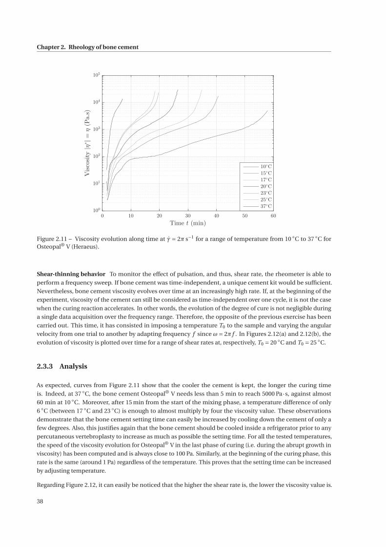
Chapter 2. Rheology of bone cement
0 10 20 30 40 50 60
Time t (min)
100
101
102
103
104
105
Viscosity|η
∗|=
η(Pa.s)
10◦C
15◦C
17◦C
20◦C
23◦C
25◦C
37◦C
Figure 2.11 – Viscosity evolution along time at γ = 2π s−1 for a range of temperature from 10 ◦C to 37 ◦C forOsteopal® V (Heraeus).
Shear-thinning behavior To monitor the effect of pulsation, and thus, shear rate, the rheometer is able to
perform a frequency sweep. If bone cement was time-independent, a unique cement kit would be sufficient.
Nevertheless, bone cement viscosity evolves over time at an increasingly high rate. If, at the beginning of the
experiment, viscosity of the cement can still be considered as time-independent over one cycle, it is not the case
when the curing reaction accelerates. In other words, the evolution of the degree of cure is not negligible during
a single data acquisition over the frequency range. Therefore, the opposite of the previous exercise has been
carried out. This time, it has consisted in imposing a temperature T0 to the sample and varying the angular
velocity from one trial to another by adapting frequency f since ω= 2π f . In Figures 2.12(a) and 2.12(b), the
evolution of viscosity is plotted over time for a range of shear rates at, respectively, T0 = 20 ◦C and T0 = 25 ◦C.
2.3.3 Analysis
As expected, curves from Figure 2.11 show that the cooler the cement is kept, the longer the curing time
is. Indeed, at 37 ◦C, the bone cement Osteopal® V needs less than 5 min to reach 5000 Pa·s, against almost
60 min at 10 ◦C. Moreover, after 15 min from the start of the mixing phase, a temperature difference of only
6 ◦C (between 17 ◦C and 23 ◦C) is enough to almost multiply by four the viscosity value. These observations
demonstrate that the bone cement setting time can easily be increased by cooling down the cement of only a
few degrees. Also, this justifies again that the bone cement should be cooled inside a refrigerator prior to any
percutaneous vertebroplasty to increase as much as possible the setting time. For all the tested temperatures,
the speed of the viscosity evolution for Osteopal® V in the last phase of curing (i.e. during the abrupt growth in
viscosity) has been computed and is always close to 100 Pa. Similarly, at the beginning of the curing phase, this
rate is the same (around 1 Pa) regardless of the temperature. This proves that the setting time can be increased
by adjusting temperature.
Regarding Figure 2.12, it can easily be noticed that the higher the shear rate is, the lower the viscosity value is.
38
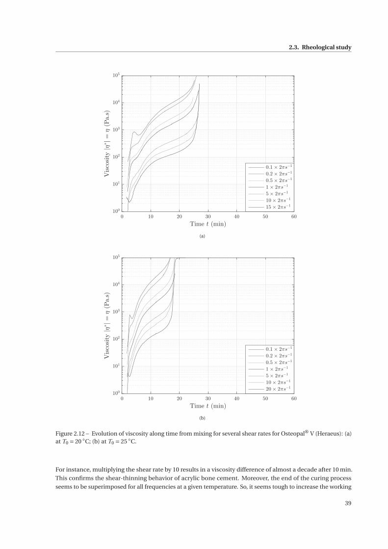
2.3. Rheological study
0 10 20 30 40 50 60
Time t (min)
100
101
102
103
104
105
Viscosity|η
∗|=
η(Pa.s)
0.1 × 2πs−1
0.2 × 2πs−1
0.5 × 2πs−1
1 × 2πs−1
5 × 2πs−1
10 × 2πs−1
15 × 2πs−1
(a)
0 10 20 30 40 50 60
Time t (min)
100
101
102
103
104
105
Viscosity|η
∗|=
η(Pa.s)
0.1 × 2πs−1
0.2 × 2πs−1
0.5 × 2πs−1
1 × 2πs−1
5 × 2πs−1
10 × 2πs−1
20 × 2πs−1
(b)
Figure 2.12 – Evolution of viscosity along time from mixing for several shear rates for Osteopal® V (Heraeus): (a)at T0 = 20 ◦C; (b) at T0 = 25 ◦C.
For instance, multiplying the shear rate by 10 results in a viscosity difference of almost a decade after 10 min.
This confirms the shear-thinning behavior of acrylic bone cement. Moreover, the end of the curing process
seems to be superimposed for all frequencies at a given temperature. So, it seems tough to increase the working
39

Chapter 2. Rheology of bone cement
phase beyond a certain time period (around 27 min at 20 ◦C and 18 min at 25 ◦C) even if the sample is highly
sheared, for instance at around γ= 100 s−1. The curves do not reach the same maximum viscosity value. This
phenomenon results from the slippage of the bone cement during the experiments. Indeed, if the adherence
between the rotating plate and the cement is not sufficient to transfer the shear stress to the rotor axis, the
output measure is insignificant.
While the full study has been completed on the cement Osteopal® V, generously provided by Heraeus, the
approach and the results are fully transposable to other bone cements. Indeed, these trends have been confirmed
for two other bone cements from Optimed as exposed in Figure 2.13 with plots of viscosity.
0 10 20 30 40 50
Time t (min)
0
2000
4000
6000
8000
10000
Viscosity|η
∗|=
η(Pa.s)
17◦C
20◦C
23◦C
(a)
0 5 10 15 20
Time t (min)
0
0.5
1
1.5
2
2.5
3
3.5
4
Viscosity|η
∗|=
η(Pa.s)
×104
0.1× 2πs−1
1× 2πs−1
10× 2πs−1
(b)
Figure 2.13 – Evolution of viscosity along time from mixing for CementoFixx-R (straight lines) and CementoFixx-M (dashed curves): (a) for a range of temperature at γ= 2π s−1; (b) for several shear rates at T0 = 20 ◦C.
In the light of the conducted experiments, viscosity can be adjusted in a controlled way by acting either on the
bone cement temperature or on shear rate during the injection. Increasing the shear rate, i.e. the bone cement
injection speed, of the bone cement decreases its viscosity. Since the injection speed should be left to the decision
of the practitioner, it is not possible to play on shear rate. For that reason, we chose to control the cement
temperature in order to meet the requirement of both reducing the leakage risk and increasing the working
phase. This will be detailed in Chapter 5. This regulation can be achieved by modulating thinly the thermal
amplitude, which is recommended to minimize the impact of the viscosity regulation on the surrounding tissues.
This control is challenging since the managed fluid is flowing and undergoes an exothermic polymerization
reaction.
40
3 Modeling and identification of bone ce-ment viscosity
Contents
3.1 Modified Power law . . . . . . . . . . . . . . . . . . . . . . . . . . . . . . . . . . . . . . . . . . . . . . . 42
3.1.1 Motivation and contributions . . . . . . . . . . . . . . . . . . . . . . . . . . . . . . . . . . . . . 42
3.1.2 Identification of the functions n and K . . . . . . . . . . . . . . . . . . . . . . . . . . . . . . . 42
3.1.3 Temperature influence . . . . . . . . . . . . . . . . . . . . . . . . . . . . . . . . . . . . . . . . . 45
3.1.4 Validation . . . . . . . . . . . . . . . . . . . . . . . . . . . . . . . . . . . . . . . . . . . . . . . . 49
3.2 Differential equation . . . . . . . . . . . . . . . . . . . . . . . . . . . . . . . . . . . . . . . . . . . . . . 50
3.2.1 Motivation and contributions . . . . . . . . . . . . . . . . . . . . . . . . . . . . . . . . . . . . . 50
3.2.2 Choice of the model . . . . . . . . . . . . . . . . . . . . . . . . . . . . . . . . . . . . . . . . . . 50
3.2.3 Phase space identification . . . . . . . . . . . . . . . . . . . . . . . . . . . . . . . . . . . . . . . 52
3.2.4 Validation . . . . . . . . . . . . . . . . . . . . . . . . . . . . . . . . . . . . . . . . . . . . . . . . 57
41
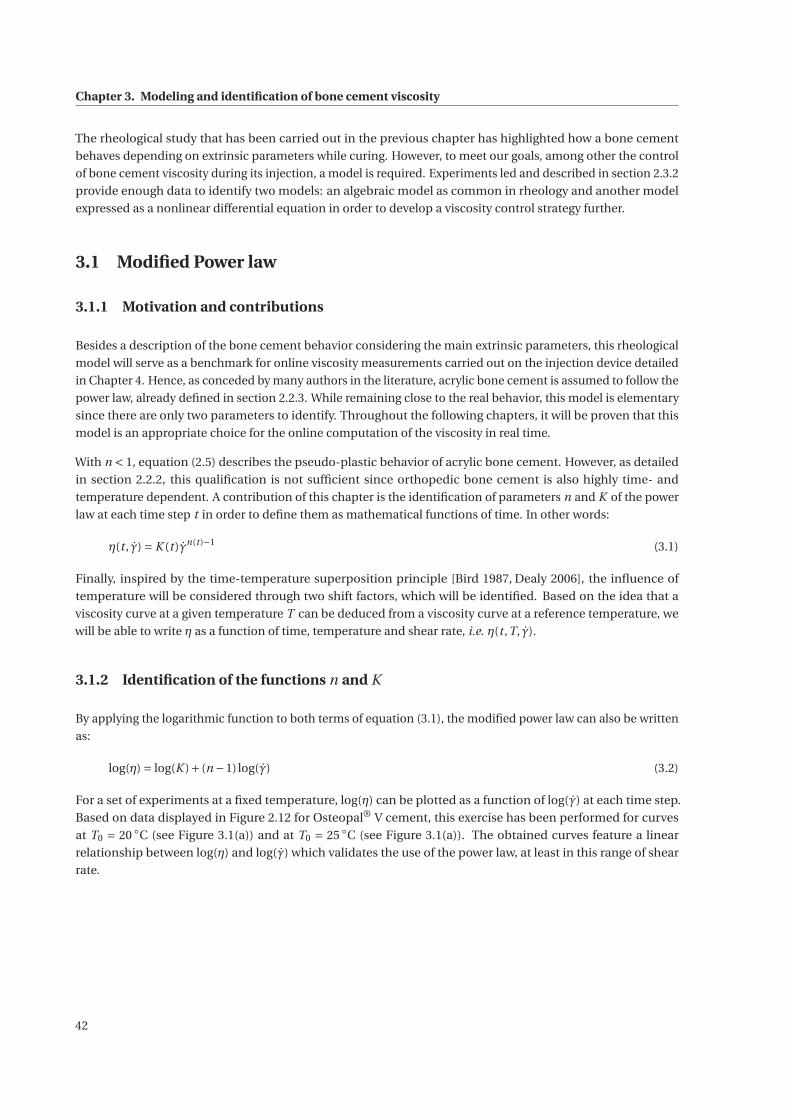
Chapter 3. Modeling and identification of bone cement viscosity
The rheological study that has been carried out in the previous chapter has highlighted how a bone cement
behaves depending on extrinsic parameters while curing. However, to meet our goals, among other the control
of bone cement viscosity during its injection, a model is required. Experiments led and described in section 2.3.2
provide enough data to identify two models: an algebraic model as common in rheology and another model
expressed as a nonlinear differential equation in order to develop a viscosity control strategy further.
3.1 Modified Power law
3.1.1 Motivation and contributions
Besides a description of the bone cement behavior considering the main extrinsic parameters, this rheological
model will serve as a benchmark for online viscosity measurements carried out on the injection device detailed
in Chapter 4. Hence, as conceded by many authors in the literature, acrylic bone cement is assumed to follow the
power law, already defined in section 2.2.3. While remaining close to the real behavior, this model is elementary
since there are only two parameters to identify. Throughout the following chapters, it will be proven that this
model is an appropriate choice for the online computation of the viscosity in real time.
With n < 1, equation (2.5) describes the pseudo-plastic behavior of acrylic bone cement. However, as detailed
in section 2.2.2, this qualification is not sufficient since orthopedic bone cement is also highly time- and
temperature dependent. A contribution of this chapter is the identification of parameters n and K of the power
law at each time step t in order to define them as mathematical functions of time. In other words:
η(t , γ) = K (t )γn(t )−1 (3.1)
Finally, inspired by the time-temperature superposition principle [Bird 1987, Dealy 2006], the influence of
temperature will be considered through two shift factors, which will be identified. Based on the idea that a
viscosity curve at a given temperature T can be deduced from a viscosity curve at a reference temperature, we
will be able to write η as a function of time, temperature and shear rate, i.e. η(t ,T, γ).
3.1.2 Identification of the functions n and K
By applying the logarithmic function to both terms of equation (3.1), the modified power law can also be written
as:
log(η) = log(K )+ (n −1)log(γ) (3.2)
For a set of experiments at a fixed temperature, log(η) can be plotted as a function of log(γ) at each time step.
Based on data displayed in Figure 2.12 for Osteopal® V cement, this exercise has been performed for curves
at T0 = 20 ◦C (see Figure 3.1(a)) and at T0 = 25 ◦C (see Figure 3.1(a)). The obtained curves feature a linear
relationship between log(η) and log(γ) which validates the use of the power law, at least in this range of shear
rate.
42
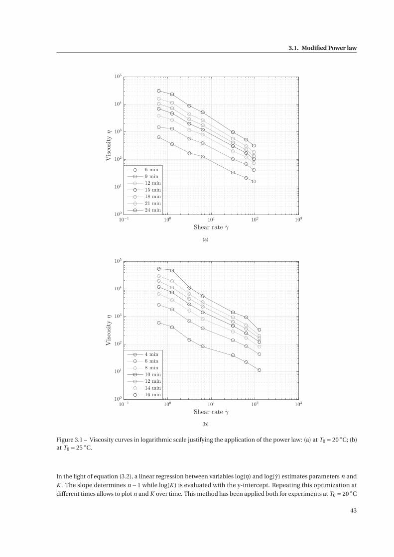
3.1. Modified Power law
10−1
100
101
102
103
Shear rate γ
100
101
102
103
104
105
Viscosityη
6 min
9 min
12 min
15 min
18 min
21 min
24 min
(a)
10−1
100
101
102
103
Shear rate γ
100
101
102
103
104
105
Viscosityη
4 min
6 min
8 min
10 min
12 min
14 min
16 min
(b)
Figure 3.1 – Viscosity curves in logarithmic scale justifying the application of the power law: (a) at T0 = 20 ◦C; (b)at T0 = 25 ◦C.
In the light of equation (3.2), a linear regression between variables log(η) and log(γ) estimates parameters n and
K . The slope determines n −1 while log(K ) is evaluated with the y-intercept. Repeating this optimization at
different times allows to plot n and K over time. This method has been applied both for experiments at T0 = 20 ◦C
43
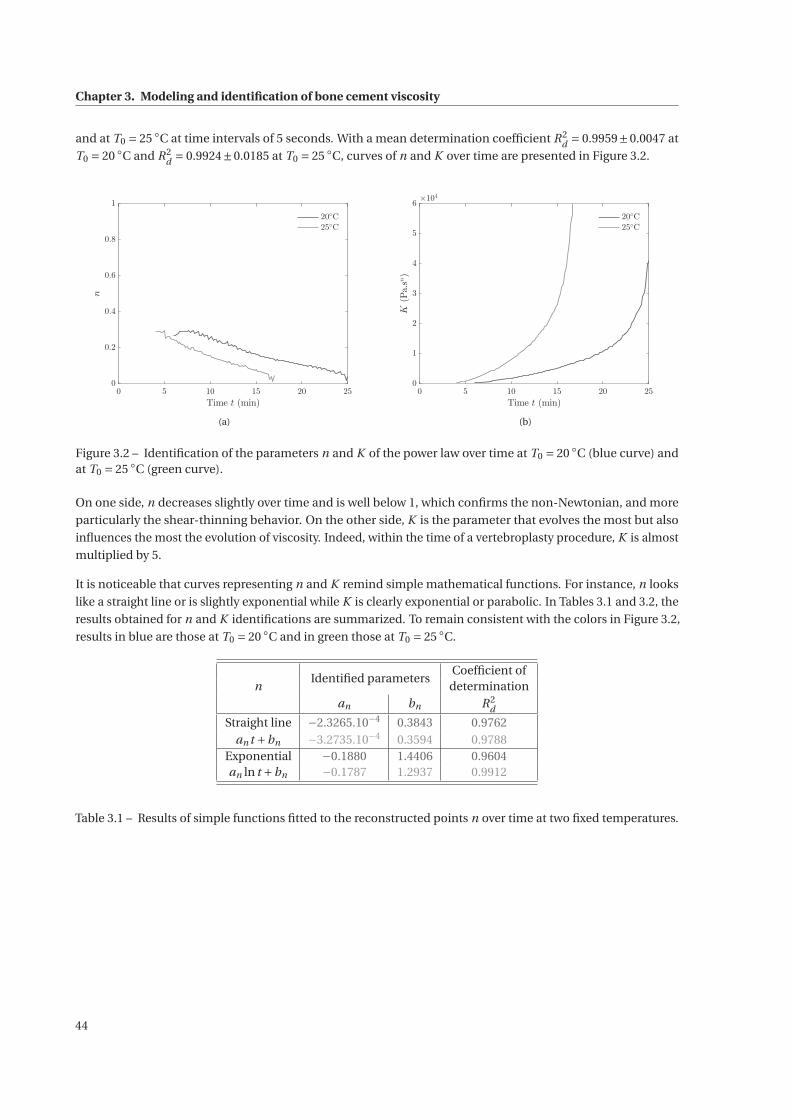
Chapter 3. Modeling and identification of bone cement viscosity
and at T0 = 25 ◦C at time intervals of 5 seconds. With a mean determination coefficient R2d = 0.9959±0.0047 at
T0 = 20 ◦C and R2d = 0.9924±0.0185 at T0 = 25 ◦C, curves of n and K over time are presented in Figure 3.2.
0 5 10 15 20 25
Time t (min)
0
0.2
0.4
0.6
0.8
1
n
20◦C
25◦C
(a)
0 5 10 15 20 25
Time t (min)
0
1
2
3
4
5
6
K(Pa.sn)
×104
20◦C
25◦C
(b)
Figure 3.2 – Identification of the parameters n and K of the power law over time at T0 = 20 ◦C (blue curve) andat T0 = 25 ◦C (green curve).
On one side, n decreases slightly over time and is well below 1, which confirms the non-Newtonian, and more
particularly the shear-thinning behavior. On the other side, K is the parameter that evolves the most but also
influences the most the evolution of viscosity. Indeed, within the time of a vertebroplasty procedure, K is almost
multiplied by 5.
It is noticeable that curves representing n and K remind simple mathematical functions. For instance, n looks
like a straight line or is slightly exponential while K is clearly exponential or parabolic. In Tables 3.1 and 3.2, the
results obtained for n and K identifications are summarized. To remain consistent with the colors in Figure 3.2,
results in blue are those at T0 = 20 ◦C and in green those at T0 = 25 ◦C.
nIdentified parameters
Coefficient ofdetermination
an bn R2d
Straight line −2.3265.10−4 0.3843 0.9762an t +bn −3.2735.10−4 0.3594 0.9788
Exponential −0.1880 1.4406 0.9604an ln t +bn −0.1787 1.2937 0.9912
Table 3.1 – Results of simple functions fitted to the reconstructed points n over time at two fixed temperatures.
44
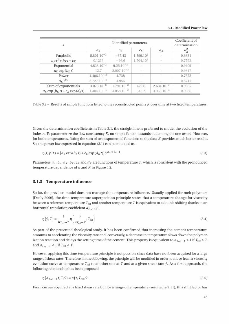
3.1. Modified Power law
KIdentified parameters
Coefficient ofdetermination
aK bK cK dK R2d
Parabolic 5.801.10−2 −67.43 1.599.104 - 0.6631aK t 2 +bK t + cK 0.1213 −96.6 1.704.104 - 0.7793
Exponential 4.623.10−2 9.25.10−3 - - 0.9409aK exp(bK t ) 12.7 8.007.10−3 - - 0.9347
Power 4.406.10−11 4.738 - - 0.7628
aK t bK 5.727.10−11 4.956 - - 0.8745
Sum of exponentials 3.078.10−8 1.791.10−2 429.6 2.684.10−3 0.9985aK exp(bK t )+ cK exp(dK t ) 1.404.10−10 3.058.10−2 545.2 3.953.10−3 0.9986
Table 3.2 – Results of simple functions fitted to the reconstructed points K over time at two fixed temperatures.
Given the determination coefficients in Table 3.1, the straight line is preferred to model the evolution of the
index n. To parameterize the flow consistency K , no simple function stands out among the one tested. However,
for both temperatures, fitting the sum of two exponential functions to the data K provides much better results.
So, the power law expressed in equation (3.1) can be modeled as:
η(t , γ,T ) =(aK exp(bK t )+ cK exp(dK t )
)γan t+bn−1. (3.3)
Parameters an , bn , aK , bK , cK and dK are functions of temperature T , which is consistent with the pronounced
temperature dependence of n and K in Figure 3.2.
3.1.3 Temperature influence
So far, the previous model does not manage the temperature influence. Usually applied for melt polymers
[Dealy 2006], the time-temperature superposition principle states that a temperature change for viscosity
between a reference temperature Tref and another temperature T is equivalent to a double shifting thanks to an
horizontal translation coefficient aTref→T :
η(γ,T
)= 1
aTref→Tη
(γ
aTref→T,Tref
)(3.4)
As part of the presented rheological study, it has been confirmed that increasing the cement temperature
amounts to accelerating the viscosity rate and, conversely, a decrease in temperature slows down the polymer-
ization reaction and delays the setting time of the cement. This property is equivalent to aTref→T > 1 if Tref > T
and aTref→T < 1 if Tref < T .
However, applying this time-temperature principle is not possible since data have not been acquired for a large
range of shear rates. Therefore, in the following, the principle will be modified in order to move from a viscosity
evolution curve at temperature Tref to another one at T and at a given shear rate γ. As a first approach, the
following relationship has been proposed:
η(aTref→T t ,T, γ
)= η
(t ,Tref, γ
)(3.5)
From curves acquired at a fixed shear rate but for a range of temperature (see Figure 2.11), this shift factor has
45
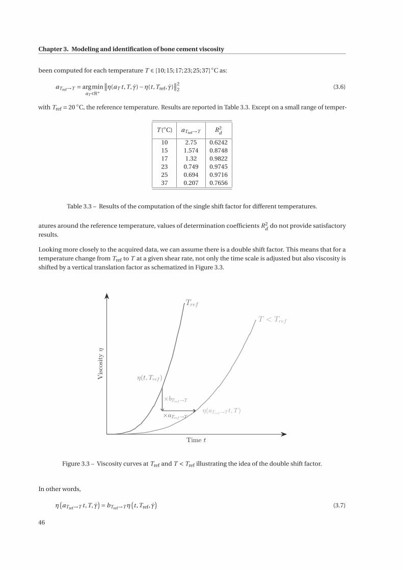
Chapter 3. Modeling and identification of bone cement viscosity
been computed for each temperature T ∈ [10;15;17;23;25;37]◦C as:
aTref→T = argminaT ∈R+
∥∥η(aT t ,T, γ)−η(t ,Tref, γ)∥∥2
2 (3.6)
with Tref = 20 ◦C, the reference temperature. Results are reported in Table 3.3. Except on a small range of temper-
T (◦C) aTref→T R2d
10 2.75 0.624215 1.574 0.874817 1.32 0.982223 0.749 0.974525 0.694 0.971637 0.207 0.7656
Table 3.3 – Results of the computation of the single shift factor for different temperatures.
atures around the reference temperature, values of determination coefficients R2d do not provide satisfactory
results.
Looking more closely to the acquired data, we can assume there is a double shift factor. This means that for a
temperature change from Tref to T at a given shear rate, not only the time scale is adjusted but also viscosity is
shifted by a vertical translation factor as schematized in Figure 3.3.
Time t
Viscosityη
Tref
T < Tref
η(t, Tref )
η(aTref→T t, T )
×bTref→T
×aTref→T
Figure 3.3 – Viscosity curves at Tref and T < Tref illustrating the idea of the double shift factor.
In other words,
η(aTref→T t ,T, γ
)= bTref→T η
(t ,Tref, γ
)(3.7)
46
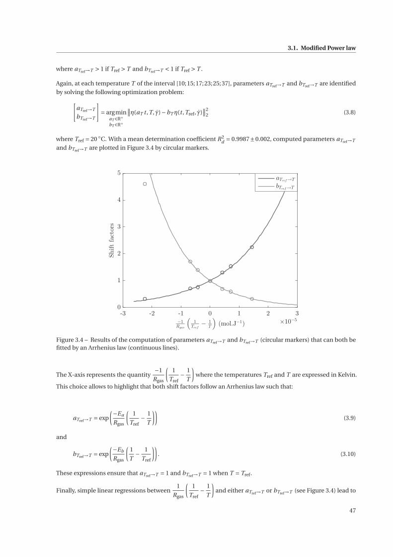
3.1. Modified Power law
where aTref→T > 1 if Tref > T and bTref→T < 1 if Tref > T .
Again, at each temperature T of the interval [10;15;17;23;25;37], parameters aTref→T and bTref→T are identified
by solving the following optimization problem:[aTref→T
bTref→T
]= argmin
aT ∈R+bT ∈R+
∥∥η(aT t ,T, γ)−bT η(t ,Tref, γ)∥∥2
2 (3.8)
where Tref = 20 ◦C. With a mean determination coefficient R2d = 0.9987±0.002, computed parameters aTref→T
and bTref→T are plotted in Figure 3.4 by circular markers.
-3 -2 -1 0 1 2 3
−1
Rgas
(1
Tref
−1
T
)(mol.J
−1) ×10
−5
0
1
2
3
4
5
Shiftfactors
aTref→T
bTref→T
Figure 3.4 – Results of the computation of parameters aTref→T and bTref→T (circular markers) that can both befitted by an Arrhenius law (continuous lines).
The X-axis represents the quantity−1
Rgas
(1
Tref− 1
T
)where the temperatures Tref and T are expressed in Kelvin.
This choice allows to highlight that both shift factors follow an Arrhenius law such that:
aTref→T = exp
(−Ea
Rgas
(1
Tref− 1
T
))(3.9)
and
bTref→T = exp
(−Eb
Rgas
(1
T− 1
Tref
)). (3.10)
These expressions ensure that aTref→T = 1 and bTref→T = 1 when T = Tref.
Finally, simple linear regressions between1
Rgas
(1
Tref− 1
T
)and either aTref→T or bTref→T (see Figure 3.4) lead to
47
Chapter 3. Modeling and identification of bone cement viscosity
the identification of the activation energies Ea and Eb as summarized in Table 3.4. These identified functions,
aTref→T and bTref→T , are drawn with straight lines in Figure 3.4.
Parameters Values SI units
Ea 5.70×10⁴ J ·mol−1
Eb 7.75×10⁴ J ·mol−1
Table 3.4 – Resulting activation energies of the identification of aTref→T and bTref→T as Arrhenius laws.
Combining equations (3.1) and (3.7) provides the following equality:
K (aTref→T t ,T )γn(aTref→T t ,T )−1 = bTref→T K (t ,Tref)γn(t ,Tref)−1 , (3.11)
which is equivalent to:
K (aTref→T t ,T ) = bTref→T K (t ,Tref) (3.12)
and
n(aTref→T t ,T ) = n(t ,Tref). (3.13)
These two last equations show that K also presents this double shift while there is only a time rescaling for n.
These features are observable in Figure 3.2 where n and K are plotted over time for two different temperatures.
Finally, choosing Tref = 20 ◦C and referring to the identified values in Tables 3.1 and 3.2, it comes that:
an = an(20 ◦C) =−2.33.10−4 , (3.14)
bn = bn(20 ◦C) = 0.384 , (3.15)
aK = aK (20 ◦C) = 3.08.10−8 , (3.16)
bK = bK (20 ◦C) = 1.79.10−2 , (3.17)
cK = cK (20 ◦C) = 430 , (3.18)
dK = dK (20 ◦C) = 2.68.10−3 (3.19)
to finally express the final modified power law as:
η(aTref→T t ,T, γ
)= bTref→T K (t ,Tref)γ
n(t ,Tref)−1. (3.20)
with n(t ,Tref = 20◦C) = an t +bn and K (t ,Tref = 20◦C) = aK exp(bK t )+ cK exp(dK t ).
48
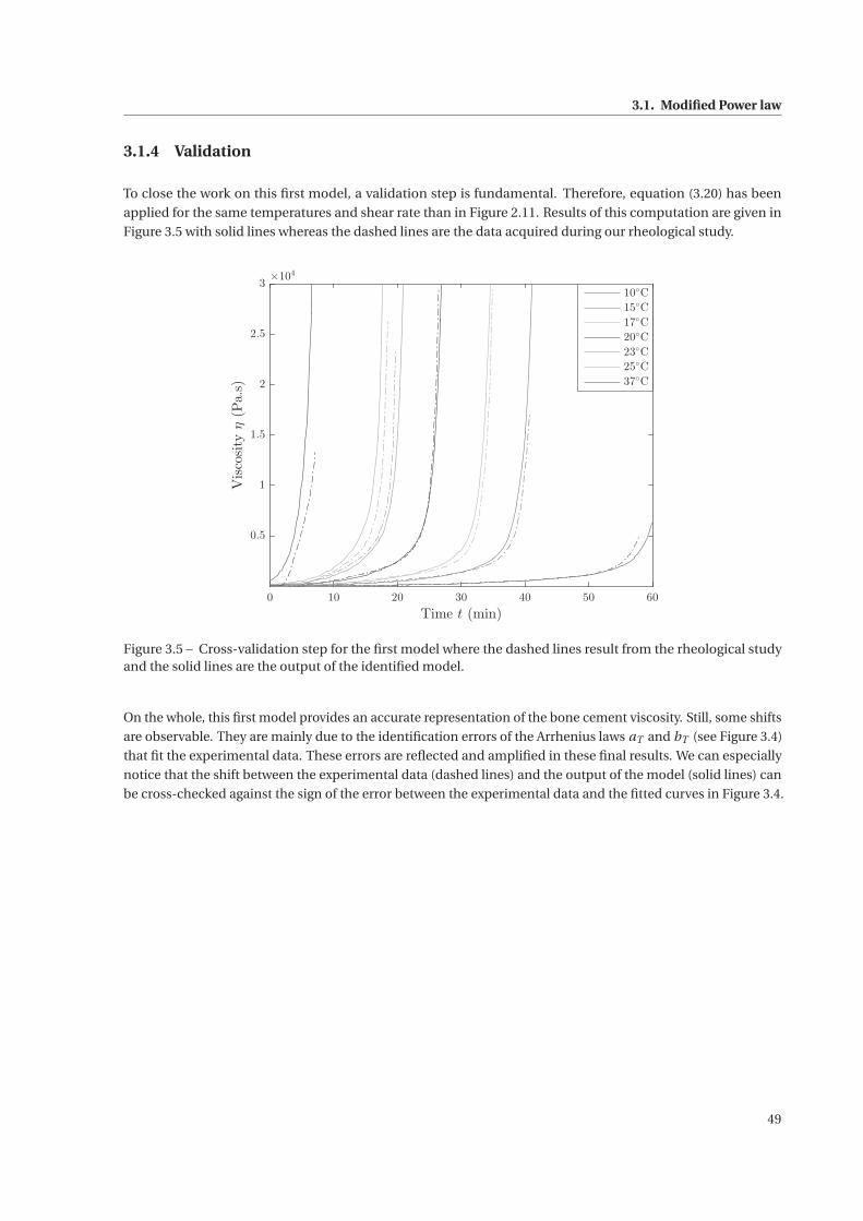
3.1. Modified Power law
3.1.4 Validation
To close the work on this first model, a validation step is fundamental. Therefore, equation (3.20) has been
applied for the same temperatures and shear rate than in Figure 2.11. Results of this computation are given in
Figure 3.5 with solid lines whereas the dashed lines are the data acquired during our rheological study.
0 10 20 30 40 50 60
Time t (min)
0.5
1
1.5
2
2.5
3
Viscosityη(Pa.s)
×104
10◦C
15◦C
17◦C
20◦C
23◦C
25◦C
37◦C
Figure 3.5 – Cross-validation step for the first model where the dashed lines result from the rheological studyand the solid lines are the output of the identified model.
On the whole, this first model provides an accurate representation of the bone cement viscosity. Still, some shifts
are observable. They are mainly due to the identification errors of the Arrhenius laws aT and bT (see Figure 3.4)
that fit the experimental data. These errors are reflected and amplified in these final results. We can especially
notice that the shift between the experimental data (dashed lines) and the output of the model (solid lines) can
be cross-checked against the sign of the error between the experimental data and the fitted curves in Figure 3.4.
49
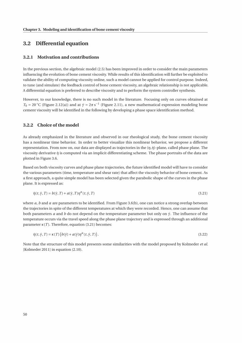
Chapter 3. Modeling and identification of bone cement viscosity
3.2 Differential equation
3.2.1 Motivation and contributions
In the previous section, the algebraic model (2.5) has been improved in order to consider the main parameters
influencing the evolution of bone cement viscosity. While results of this identification will further be exploited to
validate the ability of computing viscosity online, such a model cannot be applied for control purpose. Indeed,
to tune (and simulate) the feedback control of bone cement viscosity, an algebraic relationship is not applicable.
A differential equation is preferred to describe viscosity and to perform the system controller synthesis.
However, to our knowledge, there is no such model in the literature. Focusing only on curves obtained at
T0 = 20 ◦C (Figure 2.12(a)) and at γ = 2π s−1 (Figure 2.11), a new mathematical expression modeling bone
cement viscosity will be identified in the following by developing a phase space identification method.
3.2.2 Choice of the model
As already emphasized in the literature and observed in our rheological study, the bone cement viscosity
has a nonlinear time behavior. In order to better visualize this nonlinear behavior, we propose a different
representation. From now on, our data are displayed as trajectories in the (η, η)-plane, called phase plane. The
viscosity derivative η is computed via an implicit differentiating scheme. The phase portraits of the data are
plotted in Figure 3.6.
Based on both viscosity curves and phase plane trajectories, the future identified model will have to consider
the various parameters (time, temperature and shear rate) that affect the viscosity behavior of bone cement. As
a first approach, a quite simple model has been selected given the parabolic shape of the curves in the phase
plane. It is expressed as:
η(t , γ,T ) = b(γ,T )+a(γ,T )ηα(t , γ,T ) (3.21)
where a, b and α are parameters to be identified. From Figure 3.6(b), one can notice a strong overlap between
the trajectories in spite of the different temperatures at which they were recorded. Hence, one can assume that
both parameters a and b do not depend on the temperature parameter but only on γ. The influence of the
temperature occurs via the travel speed along the phase plane trajectory and is expressed through an additional
parameter κ(T ). Therefore, equation (3.21) becomes:
η(t , γ,T ) = κ(T )(b(γ)+a(γ)ηα(t , γ,T )
). (3.22)
Note that the structure of this model presents some similarities with the model proposed by Kolmeder et al.
[Kolmeder 2011] in equation (2.10).
50
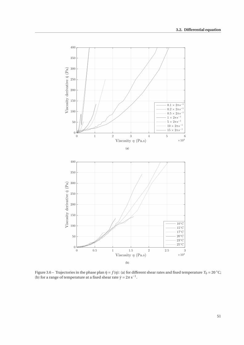
3.2. Differential equation
0 1 2 3 4 5 6
Viscosity η (Pa.s) ×104
0
50
100
150
200
250
300
350
400
Viscosityderivativeη(Pa)
0.1 × 2πs−1
0.2 × 2πs−1
0.5 × 2πs−1
1 × 2πs−1
5 × 2πs−1
10 × 2πs−1
15 × 2πs−1
(a)
0 0.5 1 1.5 2 2.5 3
Viscosity η (Pa.s) ×104
0
50
100
150
200
250
300
350
400
Viscosityderivativeη(Pa)
10◦C
15◦C
17◦C
20◦C
23◦C
25◦C
(b)
Figure 3.6 – Trajectories in the phase plan η= f (η): (a) for different shear rates and fixed temperature T0 = 20 ◦C;(b) for a range of temperature at a fixed shear rate γ= 2π s−1.
51
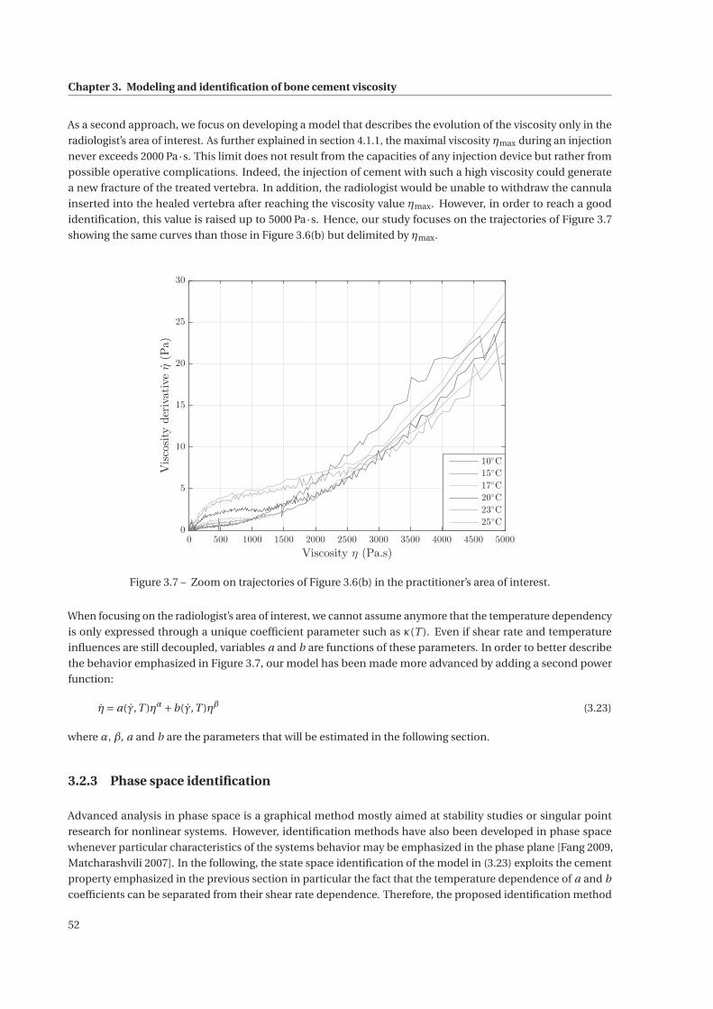
Chapter 3. Modeling and identification of bone cement viscosity
As a second approach, we focus on developing a model that describes the evolution of the viscosity only in the
radiologist’s area of interest. As further explained in section 4.1.1, the maximal viscosity ηmax during an injection
never exceeds 2000 Pa·s. This limit does not result from the capacities of any injection device but rather from
possible operative complications. Indeed, the injection of cement with such a high viscosity could generate
a new fracture of the treated vertebra. In addition, the radiologist would be unable to withdraw the cannula
inserted into the healed vertebra after reaching the viscosity value ηmax. However, in order to reach a good
identification, this value is raised up to 5000 Pa·s. Hence, our study focuses on the trajectories of Figure 3.7
showing the same curves than those in Figure 3.6(b) but delimited by ηmax.
0 500 1000 1500 2000 2500 3000 3500 4000 4500 5000
Viscosity η (Pa.s)
0
5
10
15
20
25
30
Viscosityderivativeη(Pa)
10◦C
15◦C
17◦C
20◦C
23◦C
25◦C
Figure 3.7 – Zoom on trajectories of Figure 3.6(b) in the practitioner’s area of interest.
When focusing on the radiologist’s area of interest, we cannot assume anymore that the temperature dependency
is only expressed through a unique coefficient parameter such as κ(T ). Even if shear rate and temperature
influences are still decoupled, variables a and b are functions of these parameters. In order to better describe
the behavior emphasized in Figure 3.7, our model has been made more advanced by adding a second power
function:
η= a(γ,T )ηα+b(γ,T )ηβ (3.23)
where α, β, a and b are the parameters that will be estimated in the following section.
3.2.3 Phase space identification
Advanced analysis in phase space is a graphical method mostly aimed at stability studies or singular point
research for nonlinear systems. However, identification methods have also been developed in phase space
whenever particular characteristics of the systems behavior may be emphasized in the phase plane [Fang 2009,
Matcharashvili 2007]. In the following, the state space identification of the model in (3.23) exploits the cement
property emphasized in the previous section in particular the fact that the temperature dependence of a and b
coefficients can be separated from their shear rate dependence. Therefore, the proposed identification method
52
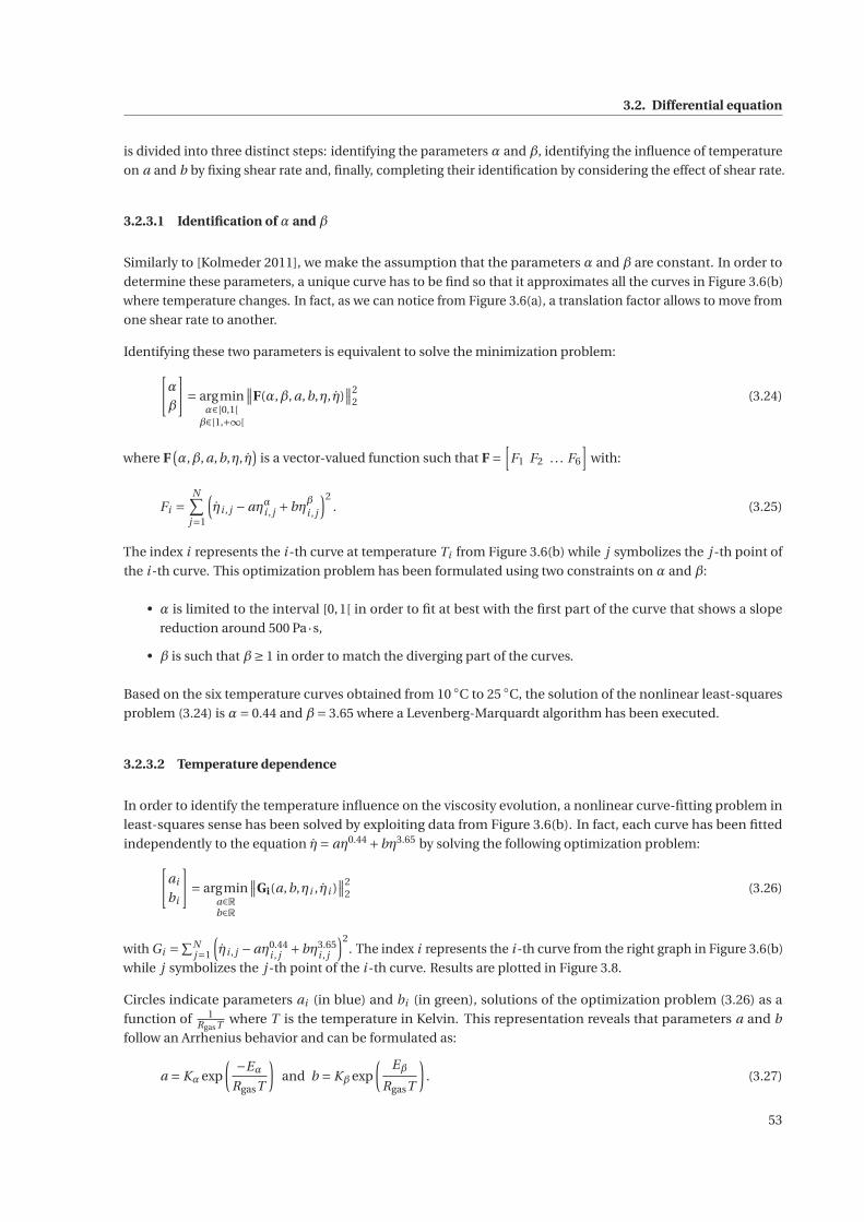
3.2. Differential equation
is divided into three distinct steps: identifying the parameters α and β, identifying the influence of temperature
on a and b by fixing shear rate and, finally, completing their identification by considering the effect of shear rate.
3.2.3.1 Identification of α and β
Similarly to [Kolmeder 2011], we make the assumption that the parameters α and β are constant. In order to
determine these parameters, a unique curve has to be find so that it approximates all the curves in Figure 3.6(b)
where temperature changes. In fact, as we can notice from Figure 3.6(a), a translation factor allows to move from
one shear rate to another.
Identifying these two parameters is equivalent to solve the minimization problem:[α
β
]= argmin
α∈[0,1[β∈[1,+∞[
∥∥F(α,β, a,b,η, η)∥∥2
2 (3.24)
where F(α,β, a,b,η, η
)is a vector-valued function such that F =
[F1 F2 . . . F6
]with:
Fi =N∑
j=1
(ηi , j −aηαi , j +bηβi , j
)2. (3.25)
The index i represents the i -th curve at temperature Ti from Figure 3.6(b) while j symbolizes the j -th point of
the i -th curve. This optimization problem has been formulated using two constraints on α and β:
• α is limited to the interval [0,1[ in order to fit at best with the first part of the curve that shows a slope
reduction around 500 Pa·s,
• β is such that β≥ 1 in order to match the diverging part of the curves.
Based on the six temperature curves obtained from 10 ◦C to 25 ◦C, the solution of the nonlinear least-squares
problem (3.24) is α= 0.44 and β= 3.65 where a Levenberg-Marquardt algorithm has been executed.
3.2.3.2 Temperature dependence
In order to identify the temperature influence on the viscosity evolution, a nonlinear curve-fitting problem in
least-squares sense has been solved by exploiting data from Figure 3.6(b). In fact, each curve has been fitted
independently to the equation η= aη0.44 +bη3.65 by solving the following optimization problem:[ai
bi
]= argmin
a∈Rb∈R
∥∥Gi(a,b,ηi , ηi )∥∥2
2 (3.26)
with Gi =∑N
j=1
(ηi , j −aη0.44
i , j +bη3.65i , j
)2. The index i represents the i -th curve from the right graph in Figure 3.6(b)
while j symbolizes the j -th point of the i -th curve. Results are plotted in Figure 3.8.
Circles indicate parameters ai (in blue) and bi (in green), solutions of the optimization problem (3.26) as a
function of 1RgasT where T is the temperature in Kelvin. This representation reveals that parameters a and b
follow an Arrhenius behavior and can be formulated as:
a = Kα exp
( −Eα
RgasT
)and b = Kβ exp
(Eβ
RgasT
). (3.27)
53
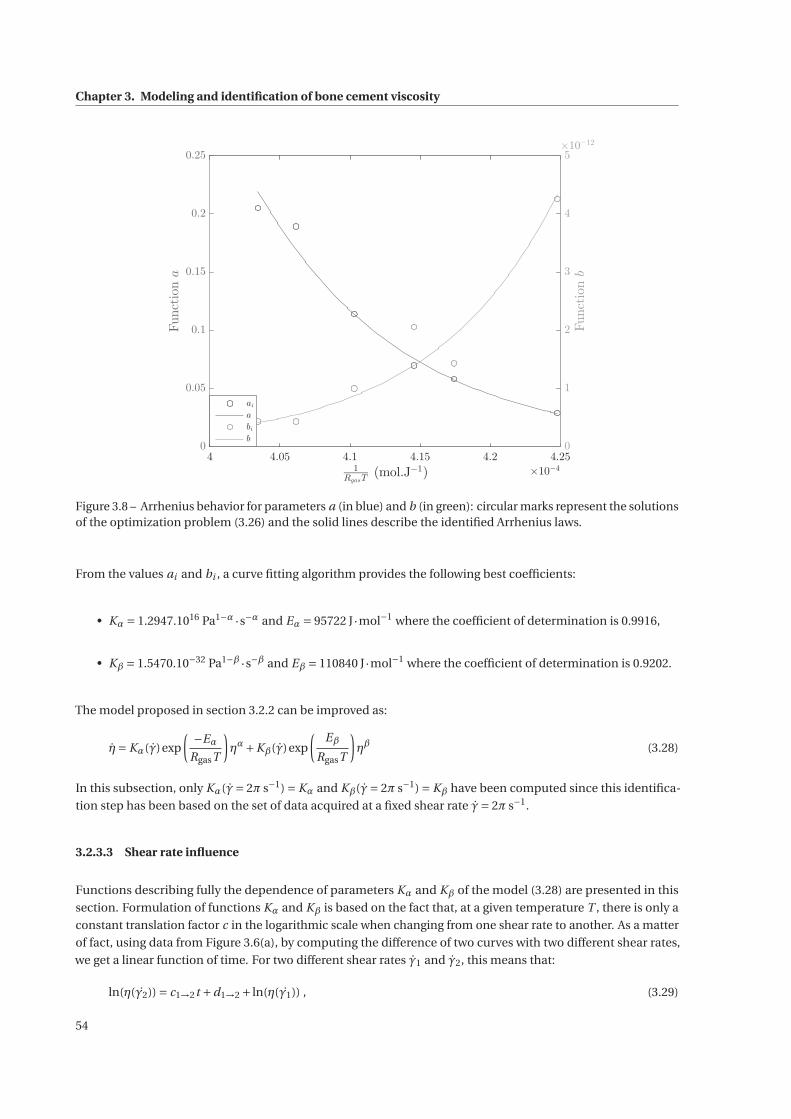
Chapter 3. Modeling and identification of bone cement viscosity
4 4.05 4.1 4.15 4.2 4.25
1
RgasT(mol.J−1) ×10
−4
0
0.05
0.1
0.15
0.2
0.25
Functiona
0
1
2
3
4
5
Functionb
×10−12
ai
a
bi
b
Figure 3.8 – Arrhenius behavior for parameters a (in blue) and b (in green): circular marks represent the solutionsof the optimization problem (3.26) and the solid lines describe the identified Arrhenius laws.
From the values ai and bi , a curve fitting algorithm provides the following best coefficients:
• Kα = 1.2947.1016 Pa1−α · s−α and Eα = 95722 J ·mol−1 where the coefficient of determination is 0.9916,
• Kβ = 1.5470.10−32 Pa1−β · s−β and Eβ = 110840 J ·mol−1 where the coefficient of determination is 0.9202.
The model proposed in section 3.2.2 can be improved as:
η= Kα(γ)exp
( −Eα
RgasT
)ηα+Kβ(γ)exp
(Eβ
RgasT
)ηβ (3.28)
In this subsection, only Kα(γ= 2π s−1) = Kα and Kβ(γ= 2π s−1) = Kβ have been computed since this identifica-
tion step has been based on the set of data acquired at a fixed shear rate γ= 2π s−1.
3.2.3.3 Shear rate influence
Functions describing fully the dependence of parameters Kα and Kβ of the model (3.28) are presented in this
section. Formulation of functions Kα and Kβ is based on the fact that, at a given temperature T , there is only a
constant translation factor c in the logarithmic scale when changing from one shear rate to another. As a matter
of fact, using data from Figure 3.6(a), by computing the difference of two curves with two different shear rates,
we get a linear function of time. For two different shear rates γ1 and γ2, this means that:
ln(η(γ2)) = c1→2t +d1→2 + ln(η(γ1)) , (3.29)
54
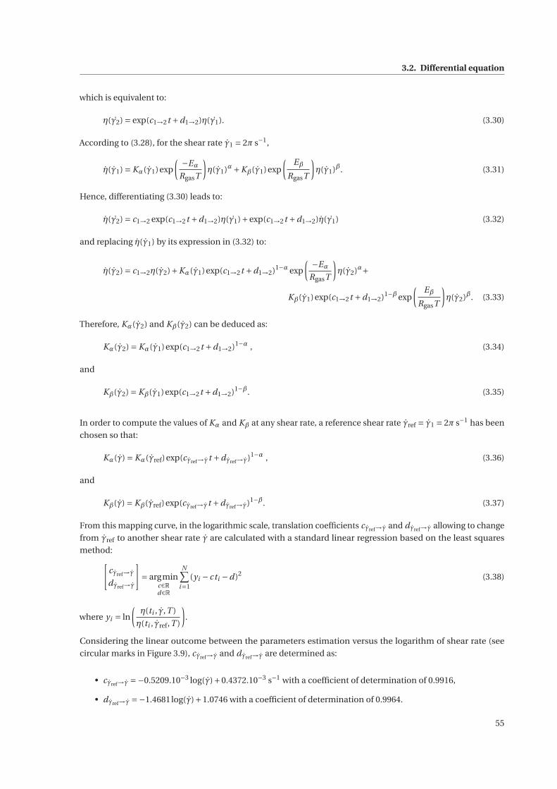
3.2. Differential equation
which is equivalent to:
η(γ2) = exp(c1→2t +d1→2)η(γ1). (3.30)
According to (3.28), for the shear rate γ1 = 2π s−1,
η(γ1) = Kα(γ1)exp
( −Eα
RgasT
)η(γ1)α+Kβ(γ1)exp
(Eβ
RgasT
)η(γ1)β. (3.31)
Hence, differentiating (3.30) leads to:
η(γ2) = c1→2 exp(c1→2t +d1→2)η(γ1)+exp(c1→2t +d1→2)η(γ1) (3.32)
and replacing η(γ1) by its expression in (3.32) to:
η(γ2) = c1→2η(γ2)+Kα(γ1)exp(c1→2t +d1→2)1−α exp
( −Eα
RgasT
)η(γ2)α+
Kβ(γ1)exp(c1→2t +d1→2)1−β exp
(Eβ
RgasT
)η(γ2)β. (3.33)
Therefore, Kα(γ2) and Kβ(γ2) can be deduced as:
Kα(γ2) = Kα(γ1)exp(c1→2t +d1→2)1−α , (3.34)
and
Kβ(γ2) = Kβ(γ1)exp(c1→2t +d1→2)1−β. (3.35)
In order to compute the values of Kα and Kβ at any shear rate, a reference shear rate γref = γ1 = 2π s−1 has been
chosen so that:
Kα(γ) = Kα(γref)exp(cγref→γt +dγref→γ)1−α , (3.36)
and
Kβ(γ) = Kβ(γref)exp(cγref→γt +dγref→γ)1−β. (3.37)
From this mapping curve, in the logarithmic scale, translation coefficients cγref→γ and dγref→γ allowing to change
from γref to another shear rate γ are calculated with a standard linear regression based on the least squares
method:[cγref→γ
dγref→γ
]= argmin
c∈Rd∈R
N∑i=1
(yi − cti −d)2 (3.38)
where yi = ln
(η(ti , γ,T )
η(ti , γref,T )
).
Considering the linear outcome between the parameters estimation versus the logarithm of shear rate (see
circular marks in Figure 3.9), cγref→γ and dγref→γ are determined as:
• cγref→γ =−0.5209.10−3 log(γ)+0.4372.10−3 s−1 with a coefficient of determination of 0.9916,
• dγref→γ =−1.4681log(γ)+1.0746 with a coefficient of determination of 0.9964.
55
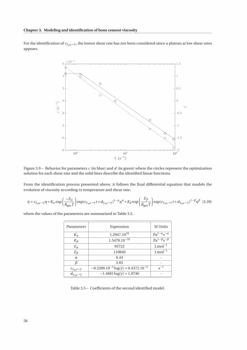
Chapter 3. Modeling and identification of bone cement viscosity
For the identification of cγref→γ, the lowest shear rate has not been considered since a plateau at low shear rates
appears.
100
101
102
γ (s−1)
-8
-6
-4
-2
0
2
4
6
c(s−1)
×10−4
-2
-1.5
-1
-0.5
0
0.5
1
1.5
-2
-1.5
-1
-0.5
0
0.5
1
1.5
d
Figure 3.9 – Behavior for parameters c (in blue) and d (in green) where the circles represent the optimizationsolution for each shear rate and the solid lines describe the identified linear functions.
From the identification process presented above, it follows the final differential equation that models the
evolution of viscosity according to temperature and shear rate:
η= cγref→γη+Kα exp
( −Eα
RgasT
)exp(cγref→γt+dγref→γ)1−αηα+Kβ exp
(Eβ
RgasT
)exp(cγref→γt+dγref→γ)1−βηβ (3.39)
where the values of the parameters are summarized in Table 3.5.
Parameters Expression SI Units
Kα 1.2947.1016 Pa1−αs−α
Kβ 1.5470.10−32 Pa1−βs−β
Eα 95722 J.mol−1
Eβ 110840 J.mol−1
α 0.44 -β 3.65 -
cγref→γ −0.5209.10−3 log(γ)+0.4372.10−3 s−1
dγref→γ −1.4681log(γ)+1.0746 -
Table 3.5 – Coefficients of the second identified model.
56
3.2. Differential equation
3.2.4 Validation
To validate this second model, the evolution of bone cement viscosity estimated by the identified differential
equation has been compared to the data acquired on the rotational rheometer. Therefore, at a given shear rate
and temperature, the nonlinear Ordinary Differential Equation (ODE) in (3.39) has been solved based on an
explicit fourth order Runge-Kutta method with a variable time step. The initial condition of this ODE equation
has been taken identical to the first viscosity value of each experimental curve.
The first validation results are those for which shear rate evolved from one experiment to another at a fixed tem-
perature T0 = 20 ◦C (Figure 3.10), and conversely, at an imposed shear rate γ= 2π s−1 for a range of temperatures
from 10 to 25 ◦C (Figure 3.11). In both figures, dashed curves are the data acquired during the rheology experi-
ments while solid lines represent the results obtained with the model, by ODE resolutions. Simulated viscosity
curves do conveniently fit the experimental data sets. Note that in Figure 3.11, a difference between ODE results
and experiments only appears above approximately 5000 Pa·s which is the maximum value considered during
the identification process.
0 10 20 30 40 50 60
Time t (min)
100
101
102
103
104
105
Viscosityη(Pa.s)
0.1 × 2πs−1
0.2 × 2πs−1
0.5 × 2πs−1
1 × 2πs−1
5 × 2πs−1
10 × 2πs−1
15 × 2πs−1
Figure 3.10 – Results obtained with the models, by solving the ODE (solid lines) in comparison with the acquiredviscosity data (dashed curves) also presented in Figure 2.12(a).
Based on data different from the ones used for the estimation step, another validation is made. Indeed, new
experimental curves have been acquired on the dynamic rheometer. While the experimental protocol detailed
in section 2.3.2.1 has carefully been followed with γ= 2π s−1 and T0 = 25 ◦C, the bone cement sample has been
cooled at a given time tc to reach the temperature T0 = 15 ◦C. Then, in Figure 3.12, in order to propose a second
validation method, each new acquired curve has been compared to the solution of equation (3.39) for which the
shear rate and temperature are identical to the ones used during the experiments.
57
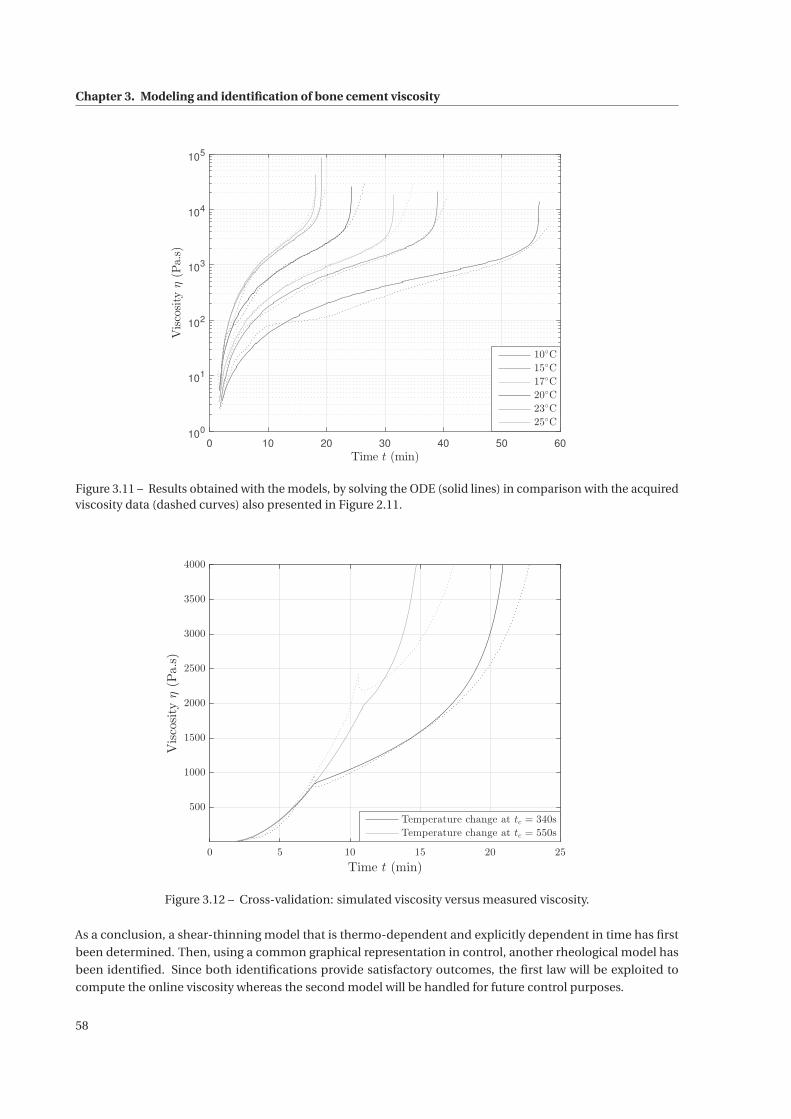
Chapter 3. Modeling and identification of bone cement viscosity
0 10 20 30 40 50 60Time t (min)
100
101
102
103
104
105
Viscosityη(Pa.s)
10◦C
15◦C
17◦C
20◦C
23◦C
25◦C
Figure 3.11 – Results obtained with the models, by solving the ODE (solid lines) in comparison with the acquiredviscosity data (dashed curves) also presented in Figure 2.11.
0 5 10 15 20 25
Time t (min)
500
1000
1500
2000
2500
3000
3500
4000
Viscosityη(Pa.s)
Temperature change at tc = 340s
Temperature change at tc = 550s
Figure 3.12 – Cross-validation: simulated viscosity versus measured viscosity.
As a conclusion, a shear-thinning model that is thermo-dependent and explicitly dependent in time has first
been determined. Then, using a common graphical representation in control, another rheological model has
been identified. Since both identifications provide satisfactory outcomes, the first law will be exploited to
compute the online viscosity whereas the second model will be handled for future control purposes.
58
4 S-Tronic robot for teleoperated bonecement injection
Contents
4.1 Robotic injection device . . . . . . . . . . . . . . . . . . . . . . . . . . . . . . . . . . . . . . . . . . . . 60
4.1.1 Design and instrumentation . . . . . . . . . . . . . . . . . . . . . . . . . . . . . . . . . . . . . 60
4.1.2 Disposable items . . . . . . . . . . . . . . . . . . . . . . . . . . . . . . . . . . . . . . . . . . . . 62
4.1.3 Passive cooling . . . . . . . . . . . . . . . . . . . . . . . . . . . . . . . . . . . . . . . . . . . . . 64
4.1.4 Control of the injection device . . . . . . . . . . . . . . . . . . . . . . . . . . . . . . . . . . . . 66
4.2 Design of a temperature control system . . . . . . . . . . . . . . . . . . . . . . . . . . . . . . . . . . . 66
4.2.1 Positioning of the temperature exchanger . . . . . . . . . . . . . . . . . . . . . . . . . . . . . 66
4.2.2 Dimensioning of the temperature exchanger . . . . . . . . . . . . . . . . . . . . . . . . . . . . 68
4.2.3 Technology of the temperature exchanger . . . . . . . . . . . . . . . . . . . . . . . . . . . . . 71
4.2.4 Validation by numerical simulations . . . . . . . . . . . . . . . . . . . . . . . . . . . . . . . . . 72
4.3 Teleoperated cement injection . . . . . . . . . . . . . . . . . . . . . . . . . . . . . . . . . . . . . . . . 74
4.3.1 Master device . . . . . . . . . . . . . . . . . . . . . . . . . . . . . . . . . . . . . . . . . . . . . . 74
4.3.2 Teleoperation background . . . . . . . . . . . . . . . . . . . . . . . . . . . . . . . . . . . . . . 75
4.3.3 Rate control strategy . . . . . . . . . . . . . . . . . . . . . . . . . . . . . . . . . . . . . . . . . . 77
4.4 Experiments . . . . . . . . . . . . . . . . . . . . . . . . . . . . . . . . . . . . . . . . . . . . . . . . . . . 79
4.4.1 Experimental set-up . . . . . . . . . . . . . . . . . . . . . . . . . . . . . . . . . . . . . . . . . . 79
4.4.2 Experimental results . . . . . . . . . . . . . . . . . . . . . . . . . . . . . . . . . . . . . . . . . . 79
59
Chapter 4. S-Tronic robot for teleoperated bone cement injection
The aim of the S-Tronic project is to help the radiologist to meet the two most important requirements of the
vertebroplasty procedure: filling the vertebral body conveniently and preventing cement leakages. To that
purpose, a robotic device has been developed, allowing the remote supervision of the cement injection, even
at high pressures. In order to assist the practitioner in limiting bone cement leakages, a fine-tuned viscosity
control is a key benefit. As a result of the rheological study presented in Chapter 2, a temperature control is an
appropriate choice to perform this viscosity control. Then, besides the visual control of the cement delivery via
real time fluoroscopic images, the curing state of the cement can be rendered by force feedback on a remote
console.
The system proposed in this Chapter combines these features. It includes an injection device that controls
the cement flow, a thermal regulation module that controls the fluid temperature, and a master interface that
provides the remote force feedback to the operator. Each of these subsystems will be detailed independently in
the following sections.
The presented mechatronic systems have been developed in the framework of the S-Tronic project. Mechanical
systems have been designed in collaboration with François Schmitt while the software engineering has been
completed by Laurent Barbé. Within this chapter, my contributions lie on the dimensioning of the different
systems, especially on the thermal regulation module.
4.1 Robotic injection device
4.1.1 Design and instrumentation
4.1.1.1 Dimensioning
Although practitioners understand the concept of viscosity thanks to sensations they experience during injec-
tions, they are not able to quantify neither the maximum viscosity threshold at which the injection should be
ended nor the minimum viscosity to be reached to avoid leakages. However, viscosity is the parameter that most
influences the pressure on the piston of the injection device. This maximum viscosity value is thus a key for the
dimensioning of our device.
Maximum viscosityηmax An experiment has been carried out on the rotational rheometer in order to determine
this threshold. The experimental protocol described in section 2.3.2.1 has again been followed with Osteopal
V® cement from Heraeus. However, if temperature has not been controlled in order to be consistent with the
current practice of vertebroplasty procedures, the shear rate for this experiment must be determined. Bone
cement has been proven to be shear-thinning, which means that the lower the shear rate is, the higher the
viscosity is. This behavior is valid above a certain shear rate and, at low shear rates, bone cement viscosity shows
a Newtonian plateau.For the dimensioning of our injection device, the worst case scenario must be considered.
Therefore, the rheological experiment has been performed at γ= 0.2×2π s−1 since, below this value, almost no
viscosity variation can be observed. At this shear rate, it allows to consider a Newtonian plateau. The resulting
viscosity evolution is plotted in Figure 4.1.
According to Figure 1.11, the working phase of the tested bone cement does not last more than 9 minutes. From
Figure 4.1, the corresponding maximum viscosity equals 1708 Pa·s, which is rounded to ηmax = 2000 Pa·s with a
safety margin of 15%.
60
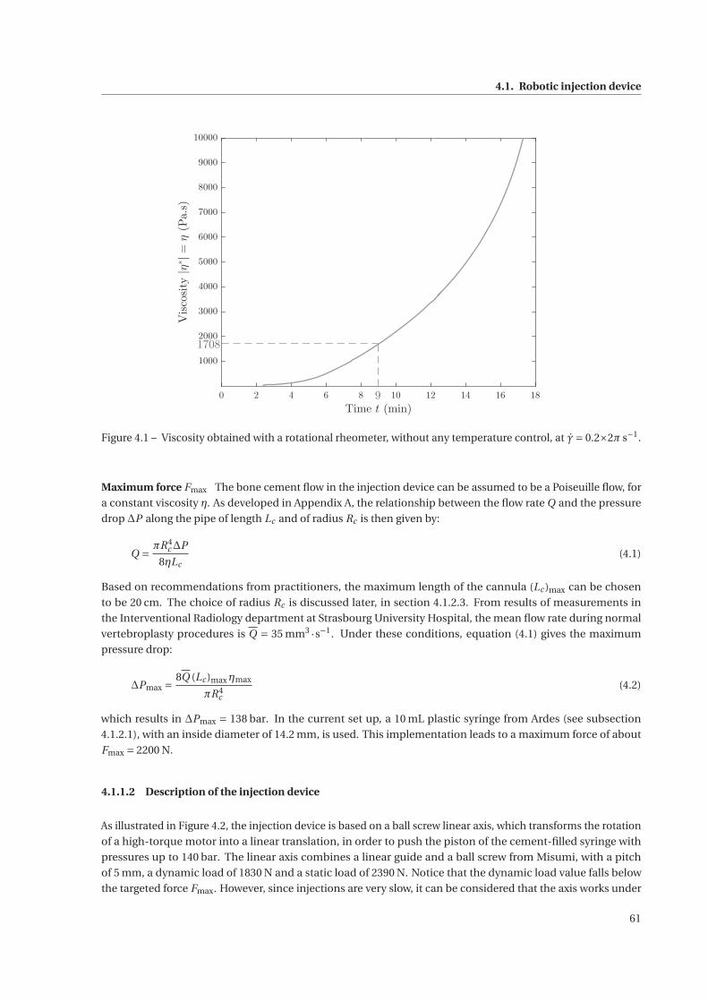
4.1. Robotic injection device
0 2 4 6 8 10 12 14 16 18
Time t (min)
1000
2000
3000
4000
5000
6000
7000
8000
9000
10000
Viscosity|η
∗|=
η(Pa.s)
9
1708
Figure 4.1 – Viscosity obtained with a rotational rheometer, without any temperature control, at γ= 0.2×2π s−1.
Maximum force Fmax The bone cement flow in the injection device can be assumed to be a Poiseuille flow, for
a constant viscosity η. As developed in Appendix A, the relationship between the flow rate Q and the pressure
drop ΔP along the pipe of length Lc and of radius Rc is then given by:
Q = πR4c ΔP
8ηLc(4.1)
Based on recommendations from practitioners, the maximum length of the cannula (Lc )max can be chosen
to be 20 cm. The choice of radius Rc is discussed later, in section 4.1.2.3. From results of measurements in
the Interventional Radiology department at Strasbourg University Hospital, the mean flow rate during normal
vertebroplasty procedures is Q = 35 mm3 ·s−1. Under these conditions, equation (4.1) gives the maximum
pressure drop:
ΔPmax =8Q (Lc )maxηmax
πR4c
(4.2)
which results in ΔPmax = 138 bar. In the current set up, a 10 mL plastic syringe from Ardes (see subsection
4.1.2.1), with an inside diameter of 14.2 mm, is used. This implementation leads to a maximum force of about
Fmax = 2200 N.
4.1.1.2 Description of the injection device
As illustrated in Figure 4.2, the injection device is based on a ball screw linear axis, which transforms the rotation
of a high-torque motor into a linear translation, in order to push the piston of the cement-filled syringe with
pressures up to 140 bar. The linear axis combines a linear guide and a ball screw from Misumi, with a pitch
of 5 mm, a dynamic load of 1830 N and a static load of 2390 N. Notice that the dynamic load value falls below
the targeted force Fmax. However, since injections are very slow, it can be considered that the axis works under
61
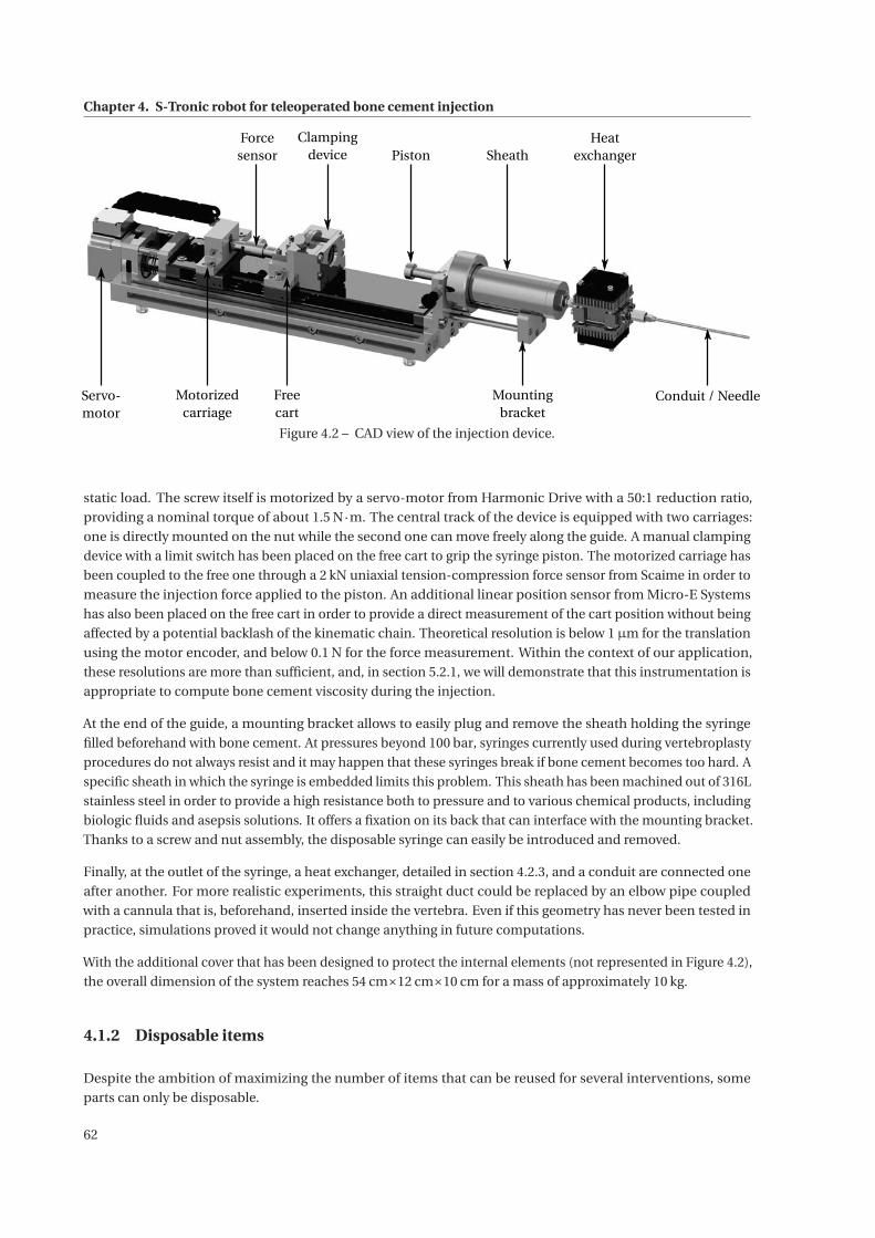
Chapter 4. S-Tronic robot for teleoperated bone cement injection
PistonClamping
device
Conduit / NeedleMotorizedcarriage
Heatexchanger
Forcesensor
Servo-motor
Freecart
Sheath
Mountingbracket
Figure 4.2 – CAD view of the injection device.
static load. The screw itself is motorized by a servo-motor from Harmonic Drive with a 50:1 reduction ratio,
providing a nominal torque of about 1.5 N·m. The central track of the device is equipped with two carriages:
one is directly mounted on the nut while the second one can move freely along the guide. A manual clamping
device with a limit switch has been placed on the free cart to grip the syringe piston. The motorized carriage has
been coupled to the free one through a 2 kN uniaxial tension-compression force sensor from Scaime in order to
measure the injection force applied to the piston. An additional linear position sensor from Micro-E Systems
has also been placed on the free cart in order to provide a direct measurement of the cart position without being
affected by a potential backlash of the kinematic chain. Theoretical resolution is below 1μm for the translation
using the motor encoder, and below 0.1 N for the force measurement. Within the context of our application,
these resolutions are more than sufficient, and, in section 5.2.1, we will demonstrate that this instrumentation is
appropriate to compute bone cement viscosity during the injection.
At the end of the guide, a mounting bracket allows to easily plug and remove the sheath holding the syringe
filled beforehand with bone cement. At pressures beyond 100 bar, syringes currently used during vertebroplasty
procedures do not always resist and it may happen that these syringes break if bone cement becomes too hard. A
specific sheath in which the syringe is embedded limits this problem. This sheath has been machined out of 316L
stainless steel in order to provide a high resistance both to pressure and to various chemical products, including
biologic fluids and asepsis solutions. It offers a fixation on its back that can interface with the mounting bracket.
Thanks to a screw and nut assembly, the disposable syringe can easily be introduced and removed.
Finally, at the outlet of the syringe, a heat exchanger, detailed in section 4.2.3, and a conduit are connected one
after another. For more realistic experiments, this straight duct could be replaced by an elbow pipe coupled
with a cannula that is, beforehand, inserted inside the vertebra. Even if this geometry has never been tested in
practice, simulations proved it would not change anything in future computations.
With the additional cover that has been designed to protect the internal elements (not represented in Figure 4.2),
the overall dimension of the system reaches 54 cm×12 cm×10 cm for a mass of approximately 10 kg.
4.1.2 Disposable items
Despite the ambition of maximizing the number of items that can be reused for several interventions, some
parts can only be disposable.
62
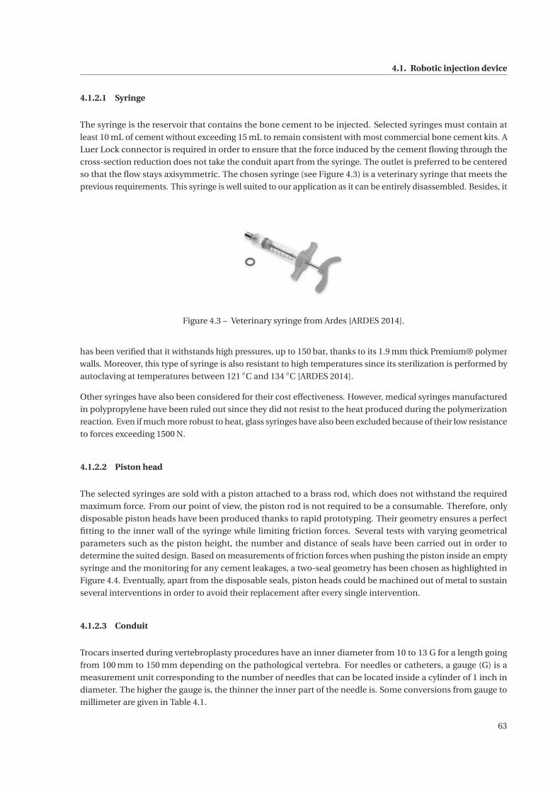
4.1. Robotic injection device
4.1.2.1 Syringe
The syringe is the reservoir that contains the bone cement to be injected. Selected syringes must contain at
least 10 mL of cement without exceeding 15 mL to remain consistent with most commercial bone cement kits. A
Luer Lock connector is required in order to ensure that the force induced by the cement flowing through the
cross-section reduction does not take the conduit apart from the syringe. The outlet is preferred to be centered
so that the flow stays axisymmetric. The chosen syringe (see Figure 4.3) is a veterinary syringe that meets the
previous requirements. This syringe is well suited to our application as it can be entirely disassembled. Besides, it
Figure 4.3 – Veterinary syringe from Ardes [ARDES 2014].
has been verified that it withstands high pressures, up to 150 bar, thanks to its 1.9 mm thick Premium® polymer
walls. Moreover, this type of syringe is also resistant to high temperatures since its sterilization is performed by
autoclaving at temperatures between 121 ◦C and 134 ◦C [ARDES 2014].
Other syringes have also been considered for their cost effectiveness. However, medical syringes manufactured
in polypropylene have been ruled out since they did not resist to the heat produced during the polymerization
reaction. Even if much more robust to heat, glass syringes have also been excluded because of their low resistance
to forces exceeding 1500 N.
4.1.2.2 Piston head
The selected syringes are sold with a piston attached to a brass rod, which does not withstand the required
maximum force. From our point of view, the piston rod is not required to be a consumable. Therefore, only
disposable piston heads have been produced thanks to rapid prototyping. Their geometry ensures a perfect
fitting to the inner wall of the syringe while limiting friction forces. Several tests with varying geometrical
parameters such as the piston height, the number and distance of seals have been carried out in order to
determine the suited design. Based on measurements of friction forces when pushing the piston inside an empty
syringe and the monitoring for any cement leakages, a two-seal geometry has been chosen as highlighted in
Figure 4.4. Eventually, apart from the disposable seals, piston heads could be machined out of metal to sustain
several interventions in order to avoid their replacement after every single intervention.
4.1.2.3 Conduit
Trocars inserted during vertebroplasty procedures have an inner diameter from 10 to 13 G for a length going
from 100 mm to 150 mm depending on the pathological vertebra. For needles or catheters, a gauge (G) is a
measurement unit corresponding to the number of needles that can be located inside a cylinder of 1 inch in
diameter. The higher the gauge is, the thinner the inner part of the needle is. Some conversions from gauge to
millimeter are given in Table 4.1.
63
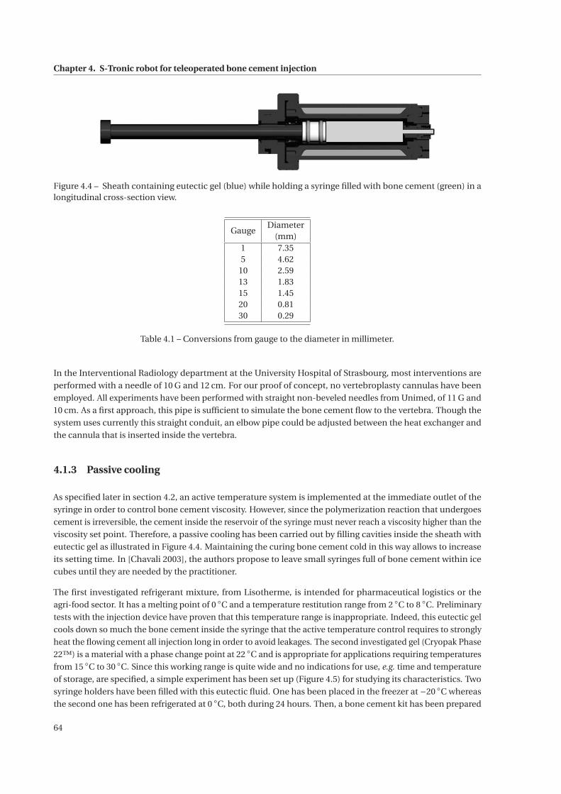
Chapter 4. S-Tronic robot for teleoperated bone cement injection
Figure 4.4 – Sheath containing eutectic gel (blue) while holding a syringe filled with bone cement (green) in alongitudinal cross-section view.
GaugeDiameter
(mm)1 7.355 4.62
10 2.5913 1.8315 1.4520 0.8130 0.29
Table 4.1 – Conversions from gauge to the diameter in millimeter.
In the Interventional Radiology department at the University Hospital of Strasbourg, most interventions are
performed with a needle of 10 G and 12 cm. For our proof of concept, no vertebroplasty cannulas have been
employed. All experiments have been performed with straight non-beveled needles from Unimed, of 11 G and
10 cm. As a first approach, this pipe is sufficient to simulate the bone cement flow to the vertebra. Though the
system uses currently this straight conduit, an elbow pipe could be adjusted between the heat exchanger and
the cannula that is inserted inside the vertebra.
4.1.3 Passive cooling
As specified later in section 4.2, an active temperature system is implemented at the immediate outlet of the
syringe in order to control bone cement viscosity. However, since the polymerization reaction that undergoes
cement is irreversible, the cement inside the reservoir of the syringe must never reach a viscosity higher than the
viscosity set point. Therefore, a passive cooling has been carried out by filling cavities inside the sheath with
eutectic gel as illustrated in Figure 4.4. Maintaining the curing bone cement cold in this way allows to increase
its setting time. In [Chavali 2003], the authors propose to leave small syringes full of bone cement within ice
cubes until they are needed by the practitioner.
The first investigated refrigerant mixture, from Lisotherme, is intended for pharmaceutical logistics or the
agri-food sector. It has a melting point of 0 ◦C and a temperature restitution range from 2 ◦C to 8 ◦C. Preliminary
tests with the injection device have proven that this temperature range is inappropriate. Indeed, this eutectic gel
cools down so much the bone cement inside the syringe that the active temperature control requires to strongly
heat the flowing cement all injection long in order to avoid leakages. The second investigated gel (Cryopak Phase
22™) is a material with a phase change point at 22 ◦C and is appropriate for applications requiring temperatures
from 15 ◦C to 30 ◦C. Since this working range is quite wide and no indications for use, e.g. time and temperature
of storage, are specified, a simple experiment has been set up (Figure 4.5) for studying its characteristics. Two
syringe holders have been filled with this eutectic fluid. One has been placed in the freezer at −20 ◦C whereas
the second one has been refrigerated at 0 ◦C, both during 24 hours. Then, a bone cement kit has been prepared
64
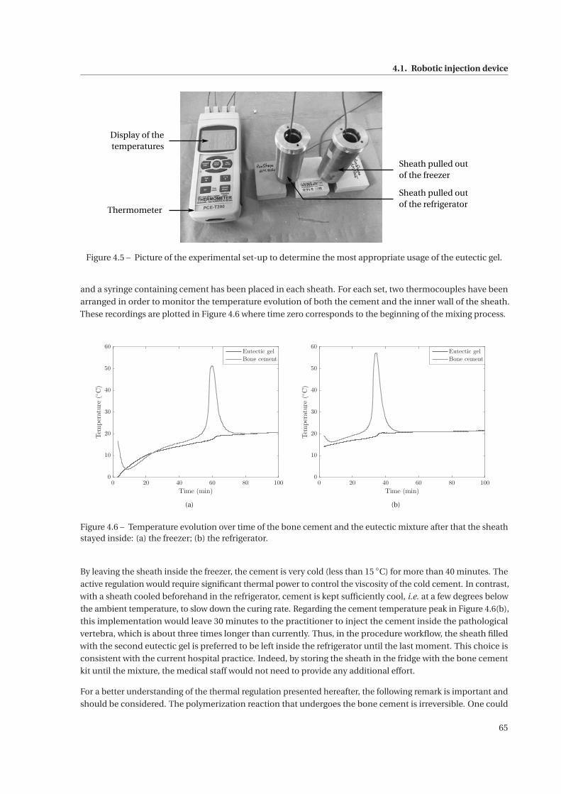
4.1. Robotic injection device
Sheath pulled outof the freezer
Sheath pulled outof the refrigerator
Thermometer
Display of thetemperatures
Figure 4.5 – Picture of the experimental set-up to determine the most appropriate usage of the eutectic gel.
and a syringe containing cement has been placed in each sheath. For each set, two thermocouples have been
arranged in order to monitor the temperature evolution of both the cement and the inner wall of the sheath.
These recordings are plotted in Figure 4.6 where time zero corresponds to the beginning of the mixing process.
0 20 40 60 80 100
Time (min)
0
10
20
30
40
50
60
Temperature(◦C)
Eutectic gel
Bone cement
(a)
0 20 40 60 80 100
Time (min)
0
10
20
30
40
50
60
Temperature(◦C)
Eutectic gel
Bone cement
(b)
Figure 4.6 – Temperature evolution over time of the bone cement and the eutectic mixture after that the sheathstayed inside: (a) the freezer; (b) the refrigerator.
By leaving the sheath inside the freezer, the cement is very cold (less than 15 ◦C) for more than 40 minutes. The
active regulation would require significant thermal power to control the viscosity of the cold cement. In contrast,
with a sheath cooled beforehand in the refrigerator, cement is kept sufficiently cool, i.e. at a few degrees below
the ambient temperature, to slow down the curing rate. Regarding the cement temperature peak in Figure 4.6(b),
this implementation would leave 30 minutes to the practitioner to inject the cement inside the pathological
vertebra, which is about three times longer than currently. Thus, in the procedure workflow, the sheath filled
with the second eutectic gel is preferred to be left inside the refrigerator until the last moment. This choice is
consistent with the current hospital practice. Indeed, by storing the sheath in the fridge with the bone cement
kit until the mixture, the medical staff would not need to provide any additional effort.
For a better understanding of the thermal regulation presented hereafter, the following remark is important and
should be considered. The polymerization reaction that undergoes the bone cement is irreversible. One could
65
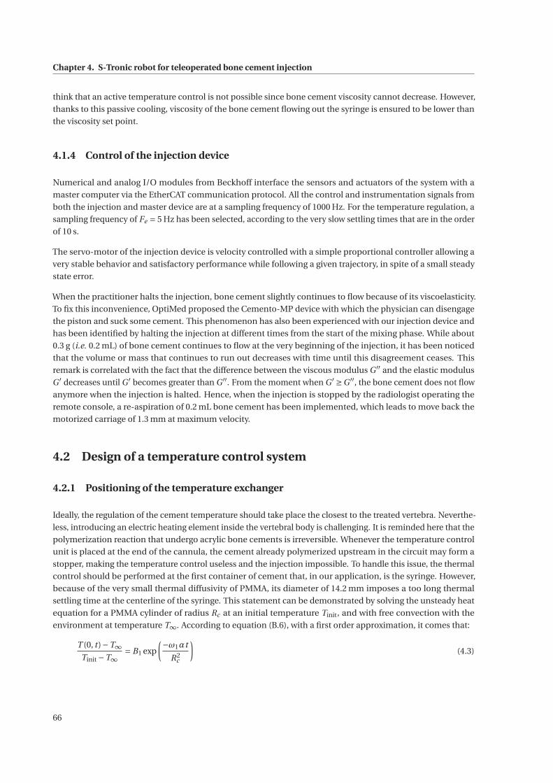
Chapter 4. S-Tronic robot for teleoperated bone cement injection
think that an active temperature control is not possible since bone cement viscosity cannot decrease. However,
thanks to this passive cooling, viscosity of the bone cement flowing out the syringe is ensured to be lower than
the viscosity set point.
4.1.4 Control of the injection device
Numerical and analog I/O modules from Beckhoff interface the sensors and actuators of the system with a
master computer via the EtherCAT communication protocol. All the control and instrumentation signals from
both the injection and master device are at a sampling frequency of 1000 Hz. For the temperature regulation, a
sampling frequency of Fe = 5 Hz has been selected, according to the very slow settling times that are in the order
of 10 s.
The servo-motor of the injection device is velocity controlled with a simple proportional controller allowing a
very stable behavior and satisfactory performance while following a given trajectory, in spite of a small steady
state error.
When the practitioner halts the injection, bone cement slightly continues to flow because of its viscoelasticity.
To fix this inconvenience, OptiMed proposed the Cemento-MP device with which the physician can disengage
the piston and suck some cement. This phenomenon has also been experienced with our injection device and
has been identified by halting the injection at different times from the start of the mixing phase. While about
0.3 g (i.e. 0.2 mL) of bone cement continues to flow at the very beginning of the injection, it has been noticed
that the volume or mass that continues to run out decreases with time until this disagreement ceases. This
remark is correlated with the fact that the difference between the viscous modulus G ′′ and the elastic modulus
G ′ decreases until G ′ becomes greater than G ′′. From the moment when G ′ ≥G ′′, the bone cement does not flow
anymore when the injection is halted. Hence, when the injection is stopped by the radiologist operating the
remote console, a re-aspiration of 0.2 mL bone cement has been implemented, which leads to move back the
motorized carriage of 1.3 mm at maximum velocity.
4.2 Design of a temperature control system
4.2.1 Positioning of the temperature exchanger
Ideally, the regulation of the cement temperature should take place the closest to the treated vertebra. Neverthe-
less, introducing an electric heating element inside the vertebral body is challenging. It is reminded here that the
polymerization reaction that undergo acrylic bone cements is irreversible. Whenever the temperature control
unit is placed at the end of the cannula, the cement already polymerized upstream in the circuit may form a
stopper, making the temperature control useless and the injection impossible. To handle this issue, the thermal
control should be performed at the first container of cement that, in our application, is the syringe. However,
because of the very small thermal diffusivity of PMMA, its diameter of 14.2 mm imposes a too long thermal
settling time at the centerline of the syringe. This statement can be demonstrated by solving the unsteady heat
equation for a PMMA cylinder of radius Rc at an initial temperature Tinit, and with free convection with the
environment at temperature T∞. According to equation (B.6), with a first order approximation, it comes that:
T (0, t )−T∞Tinit −T∞
= B1 exp
(−ω1αt
R2c
)(4.3)
66
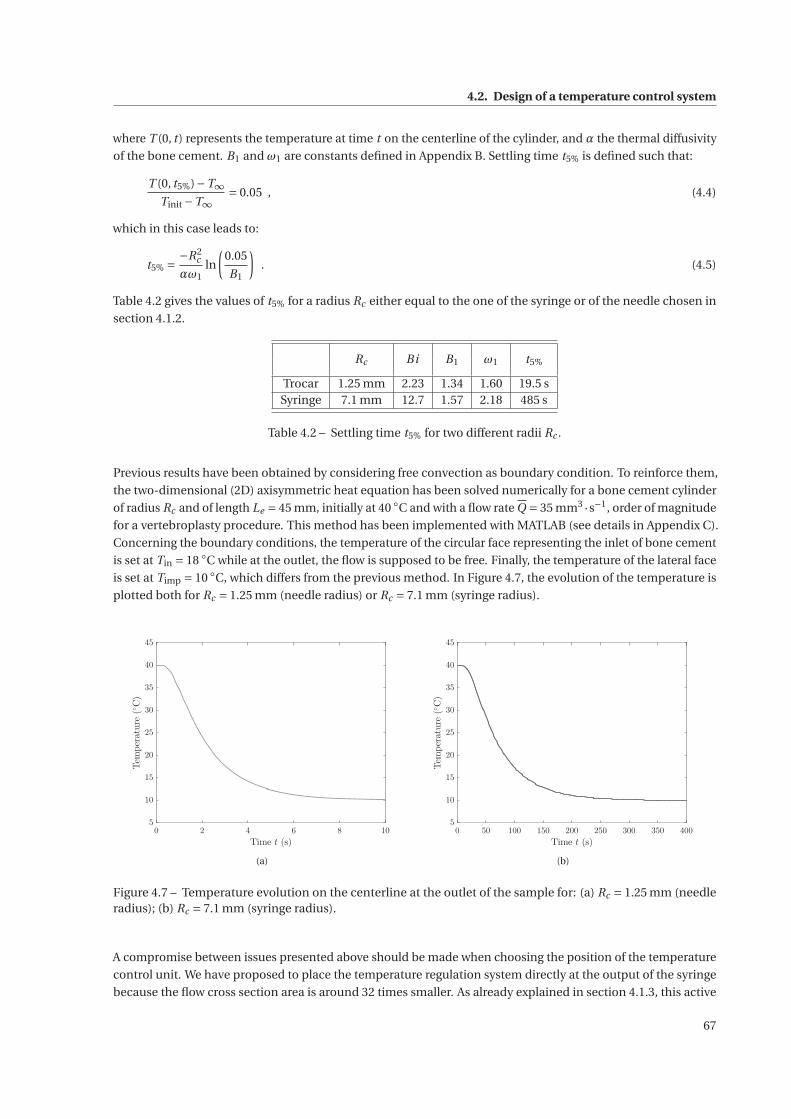
4.2. Design of a temperature control system
where T (0, t ) represents the temperature at time t on the centerline of the cylinder, and α the thermal diffusivity
of the bone cement. B1 and ω1 are constants defined in Appendix B. Settling time t5% is defined such that:
T (0, t5%)−T∞Tinit −T∞
= 0.05 , (4.4)
which in this case leads to:
t5% = −R2c
αω1ln
(0.05
B1
). (4.5)
Table 4.2 gives the values of t5% for a radius Rc either equal to the one of the syringe or of the needle chosen in
section 4.1.2.
Rc Bi B1 ω1 t5%
Trocar 1.25 mm 2.23 1.34 1.60 19.5 sSyringe 7.1 mm 12.7 1.57 2.18 485 s
Table 4.2 – Settling time t5% for two different radii Rc .
Previous results have been obtained by considering free convection as boundary condition. To reinforce them,
the two-dimensional (2D) axisymmetric heat equation has been solved numerically for a bone cement cylinder
of radius Rc and of length Le = 45 mm, initially at 40 ◦C and with a flow rate Q = 35 mm3 ·s−1, order of magnitude
for a vertebroplasty procedure. This method has been implemented with MATLAB (see details in Appendix C).
Concerning the boundary conditions, the temperature of the circular face representing the inlet of bone cement
is set at Tin = 18 ◦C while at the outlet, the flow is supposed to be free. Finally, the temperature of the lateral face
is set at Timp = 10 ◦C, which differs from the previous method. In Figure 4.7, the evolution of the temperature is
plotted both for Rc = 1.25 mm (needle radius) or Rc = 7.1 mm (syringe radius).
0 2 4 6 8 10
Time t (s)
5
10
15
20
25
30
35
40
45
Temperature(◦C)
(a)
0 50 100 150 200 250 300 350 400
Time t (s)
5
10
15
20
25
30
35
40
45
Temperature(◦C)
(b)
Figure 4.7 – Temperature evolution on the centerline at the outlet of the sample for: (a) Rc = 1.25 mm (needleradius); (b) Rc = 7.1 mm (syringe radius).
A compromise between issues presented above should be made when choosing the position of the temperature
control unit. We have proposed to place the temperature regulation system directly at the output of the syringe
because the flow cross section area is around 32 times smaller. As already explained in section 4.1.3, this active
67
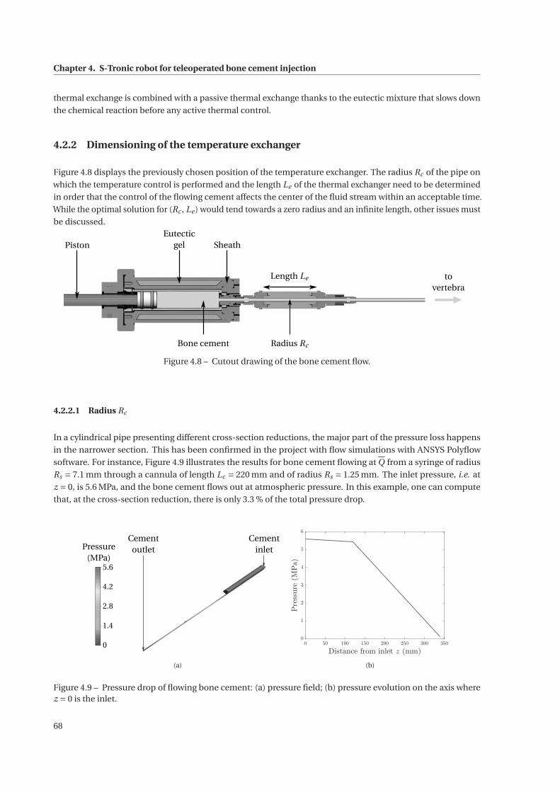
Chapter 4. S-Tronic robot for teleoperated bone cement injection
thermal exchange is combined with a passive thermal exchange thanks to the eutectic mixture that slows down
the chemical reaction before any active thermal control.
4.2.2 Dimensioning of the temperature exchanger
Figure 4.8 displays the previously chosen position of the temperature exchanger. The radius Rc of the pipe on
which the temperature control is performed and the length Le of the thermal exchanger need to be determined
in order that the control of the flowing cement affects the center of the fluid stream within an acceptable time.
While the optimal solution for (Rc , Le ) would tend towards a zero radius and an infinite length, other issues must
be discussed.
Piston
Length Le
Radius Rc
SheathEutectic
gel
Bone cement
tovertebra
Figure 4.8 – Cutout drawing of the bone cement flow.
4.2.2.1 Radius Rc
In a cylindrical pipe presenting different cross-section reductions, the major part of the pressure loss happens
in the narrower section. This has been confirmed in the project with flow simulations with ANSYS Polyflow
software. For instance, Figure 4.9 illustrates the results for bone cement flowing at Q from a syringe of radius
Rs = 7.1 mm through a cannula of length Lc = 220 mm and of radius Rs = 1.25 mm. The inlet pressure, i.e. at
z = 0, is 5.6 MPa, and the bone cement flows out at atmospheric pressure. In this example, one can compute
that, at the cross-section reduction, there is only 3.3 % of the total pressure drop.
Cementoutlet
Cementinlet
5.6
0
4.2
2.8
1.4
Pressure(MPa)
(a)
0 50 100 150 200 250 300 350
Distance from inlet z (mm)
0
1
2
3
4
5
6
Pressure(MPa)
(b)
Figure 4.9 – Pressure drop of flowing bone cement: (a) pressure field; (b) pressure evolution on the axis wherez = 0 is the inlet.
68
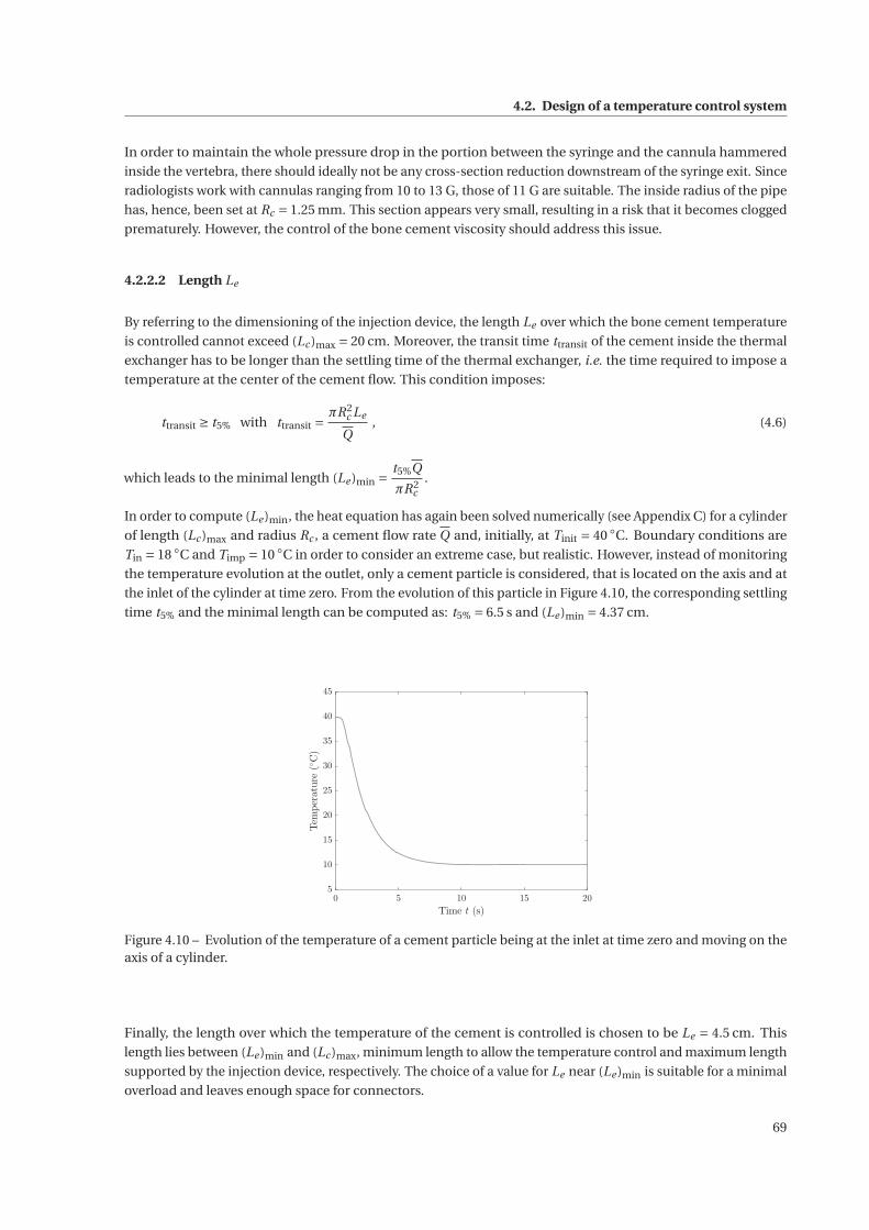
4.2. Design of a temperature control system
In order to maintain the whole pressure drop in the portion between the syringe and the cannula hammered
inside the vertebra, there should ideally not be any cross-section reduction downstream of the syringe exit. Since
radiologists work with cannulas ranging from 10 to 13 G, those of 11 G are suitable. The inside radius of the pipe
has, hence, been set at Rc = 1.25 mm. This section appears very small, resulting in a risk that it becomes clogged
prematurely. However, the control of the bone cement viscosity should address this issue.
4.2.2.2 Length Le
By referring to the dimensioning of the injection device, the length Le over which the bone cement temperature
is controlled cannot exceed (Lc )max = 20 cm. Moreover, the transit time ttransit of the cement inside the thermal
exchanger has to be longer than the settling time of the thermal exchanger, i.e. the time required to impose a
temperature at the center of the cement flow. This condition imposes:
ttransit ≥ t5% with ttransit =πR2
c Le
Q, (4.6)
which leads to the minimal length (Le )min = t5%Q
πR2c
.
In order to compute (Le )min, the heat equation has again been solved numerically (see Appendix C) for a cylinder
of length (Lc )max and radius Rc , a cement flow rate Q and, initially, at Tinit = 40 ◦C. Boundary conditions are
Tin = 18 ◦C and Timp = 10 ◦C in order to consider an extreme case, but realistic. However, instead of monitoring
the temperature evolution at the outlet, only a cement particle is considered, that is located on the axis and at
the inlet of the cylinder at time zero. From the evolution of this particle in Figure 4.10, the corresponding settling
time t5% and the minimal length can be computed as: t5% = 6.5 s and (Le )min = 4.37 cm.
0 5 10 15 20
Time t (s)
5
10
15
20
25
30
35
40
45
Temperature(◦C)
Figure 4.10 – Evolution of the temperature of a cement particle being at the inlet at time zero and moving on theaxis of a cylinder.
Finally, the length over which the temperature of the cement is controlled is chosen to be Le = 4.5 cm. This
length lies between (Le )min and (Lc )max, minimum length to allow the temperature control and maximum length
supported by the injection device, respectively. The choice of a value for Le near (Le )min is suitable for a minimal
overload and leaves enough space for connectors.
69
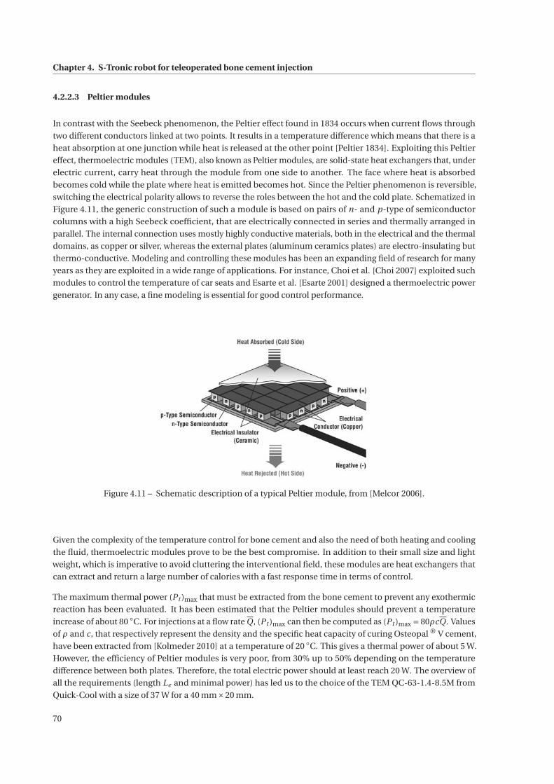
Chapter 4. S-Tronic robot for teleoperated bone cement injection
4.2.2.3 Peltier modules
In contrast with the Seebeck phenomenon, the Peltier effect found in 1834 occurs when current flows through
two different conductors linked at two points. It results in a temperature difference which means that there is a
heat absorption at one junction while heat is released at the other point [Peltier 1834]. Exploiting this Peltier
effect, thermoelectric modules (TEM), also known as Peltier modules, are solid-state heat exchangers that, under
electric current, carry heat through the module from one side to another. The face where heat is absorbed
becomes cold while the plate where heat is emitted becomes hot. Since the Peltier phenomenon is reversible,
switching the electrical polarity allows to reverse the roles between the hot and the cold plate. Schematized in
Figure 4.11, the generic construction of such a module is based on pairs of n- and p-type of semiconductor
columns with a high Seebeck coefficient, that are electrically connected in series and thermally arranged in
parallel. The internal connection uses mostly highly conductive materials, both in the electrical and the thermal
domains, as copper or silver, whereas the external plates (aluminum ceramics plates) are electro-insulating but
thermo-conductive. Modeling and controlling these modules has been an expanding field of research for many
years as they are exploited in a wide range of applications. For instance, Choi et al. [Choi 2007] exploited such
modules to control the temperature of car seats and Esarte et al. [Esarte 2001] designed a thermoelectric power
generator. In any case, a fine modeling is essential for good control performance.
Figure 4.11 – Schematic description of a typical Peltier module, from [Melcor 2006].
Given the complexity of the temperature control for bone cement and also the need of both heating and cooling
the fluid, thermoelectric modules prove to be the best compromise. In addition to their small size and light
weight, which is imperative to avoid cluttering the interventional field, these modules are heat exchangers that
can extract and return a large number of calories with a fast response time in terms of control.
The maximum thermal power (Pt )max that must be extracted from the bone cement to prevent any exothermic
reaction has been evaluated. It has been estimated that the Peltier modules should prevent a temperature
increase of about 80 ◦C. For injections at a flow rate Q, (Pt )max can then be computed as (Pt )max = 80ρcQ. Values
of ρ and c, that respectively represent the density and the specific heat capacity of curing Osteopal ® V cement,
have been extracted from [Kolmeder 2010] at a temperature of 20 ◦C. This gives a thermal power of about 5 W.
However, the efficiency of Peltier modules is very poor, from 30% up to 50% depending on the temperature
difference between both plates. Therefore, the total electric power should at least reach 20 W. The overview of
all the requirements (length Le and minimal power) has led us to the choice of the TEM QC-63-1.4-8.5M from
Quick-Cool with a size of 37 W for a 40 mm×20 mm.
70
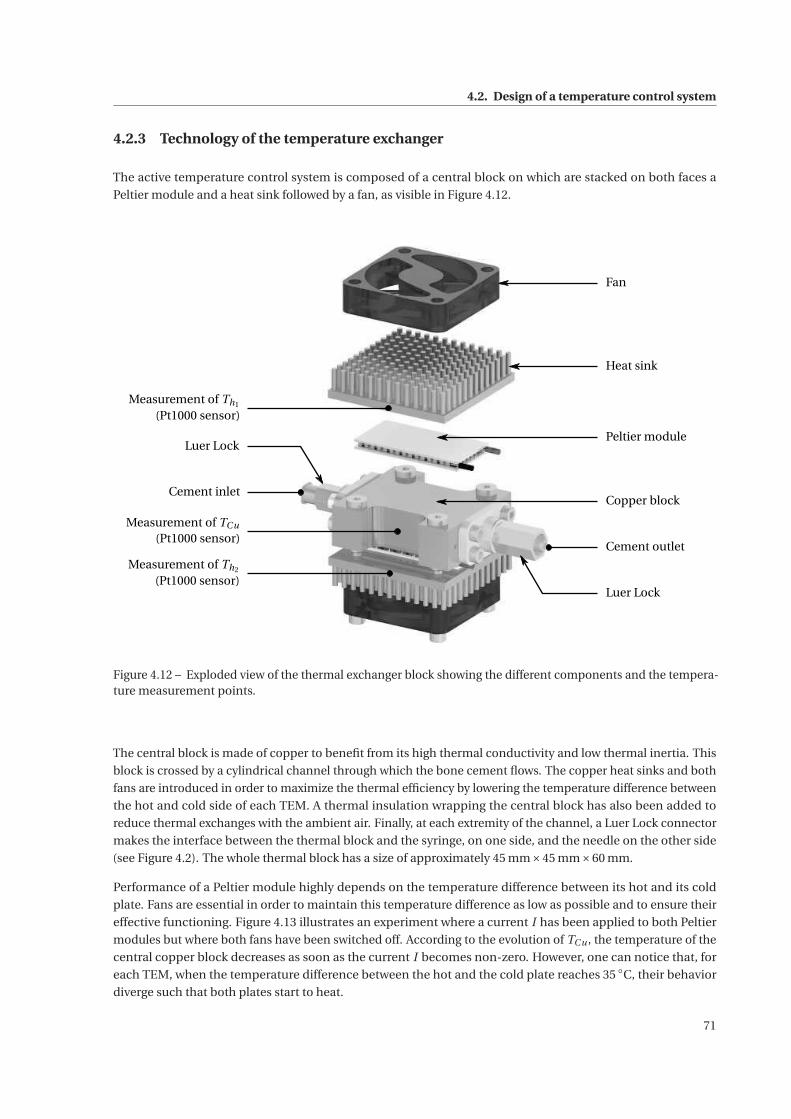
4.2. Design of a temperature control system
4.2.3 Technology of the temperature exchanger
The active temperature control system is composed of a central block on which are stacked on both faces a
Peltier module and a heat sink followed by a fan, as visible in Figure 4.12.
Fan
Heat sink
Peltier module
Copper block
Luer Lock
Cement outlet
Measurement of Th1
(Pt1000 sensor)
Cement inlet
Luer Lock
Measurement of TCu
(Pt1000 sensor)
Measurement of Th2
(Pt1000 sensor)
Figure 4.12 – Exploded view of the thermal exchanger block showing the different components and the tempera-ture measurement points.
The central block is made of copper to benefit from its high thermal conductivity and low thermal inertia. This
block is crossed by a cylindrical channel through which the bone cement flows. The copper heat sinks and both
fans are introduced in order to maximize the thermal efficiency by lowering the temperature difference between
the hot and cold side of each TEM. A thermal insulation wrapping the central block has also been added to
reduce thermal exchanges with the ambient air. Finally, at each extremity of the channel, a Luer Lock connector
makes the interface between the thermal block and the syringe, on one side, and the needle on the other side
(see Figure 4.2). The whole thermal block has a size of approximately 45 mm×45 mm×60 mm.
Performance of a Peltier module highly depends on the temperature difference between its hot and its cold
plate. Fans are essential in order to maintain this temperature difference as low as possible and to ensure their
effective functioning. Figure 4.13 illustrates an experiment where a current I has been applied to both Peltier
modules but where both fans have been switched off. According to the evolution of TCu , the temperature of the
central copper block decreases as soon as the current I becomes non-zero. However, one can notice that, for
each TEM, when the temperature difference between the hot and the cold plate reaches 35 ◦C, their behavior
diverge such that both plates start to heat.
71

Chapter 4. S-Tronic robot for teleoperated bone cement injection
0 10 20 30 40 50 60 70 80
-2
-1
0
CurrentI(A)
0 10 20 30 40 50 60 70 80
Time t (min)
10
20
30
40
50
60
70
80
Temperatures(◦C)
Th1
Th2
TCu
Figure 4.13 – Temperature measures on the thermal exchanger where both TEMs are subject to a current I withboth fans turned off.
4.2.4 Validation by numerical simulations
Prior to the assembly of the system, FEM simulations with ANSYS Polyflow software have confirmed the choice
of these Peltier modules. Especially, the settling time is ensured to be lower than the transit time of the cement
in the pipeline. They allow us to estimate the heat transfer capability and, especially, the time delay necessary to
equalize the temperature difference between each TEM cold side and the bone cement. Contrary to previous
simulations, the exact geometry of the complete thermal exchanger has been considered. Due to its symmetries,
simulations have only been carried out on a quarter of the domain (see Figure 4.14(b)). The bone cement
rheological behavior has been modeled by the power law with n = 0.2 and K = 7000 Pa·sn. The flowing cement
enters with an initial temperature and the cold face of the TEM is set at a constant temperature. For the outer
boundaries, the system is subjected to free convective heat exchange with ambient air. By computing the
temperature evolution at the outlet of the block, the settling time of the system, the delay to reach the center of
the stream and the static gain have been identified. In the example illustrated in Figure 4.14, the cement enters
at 18 ◦C and flows at Q = 35 mm3 ·s−1. The cold side of the Peltier module is supposed to be at 10 ◦C.
72
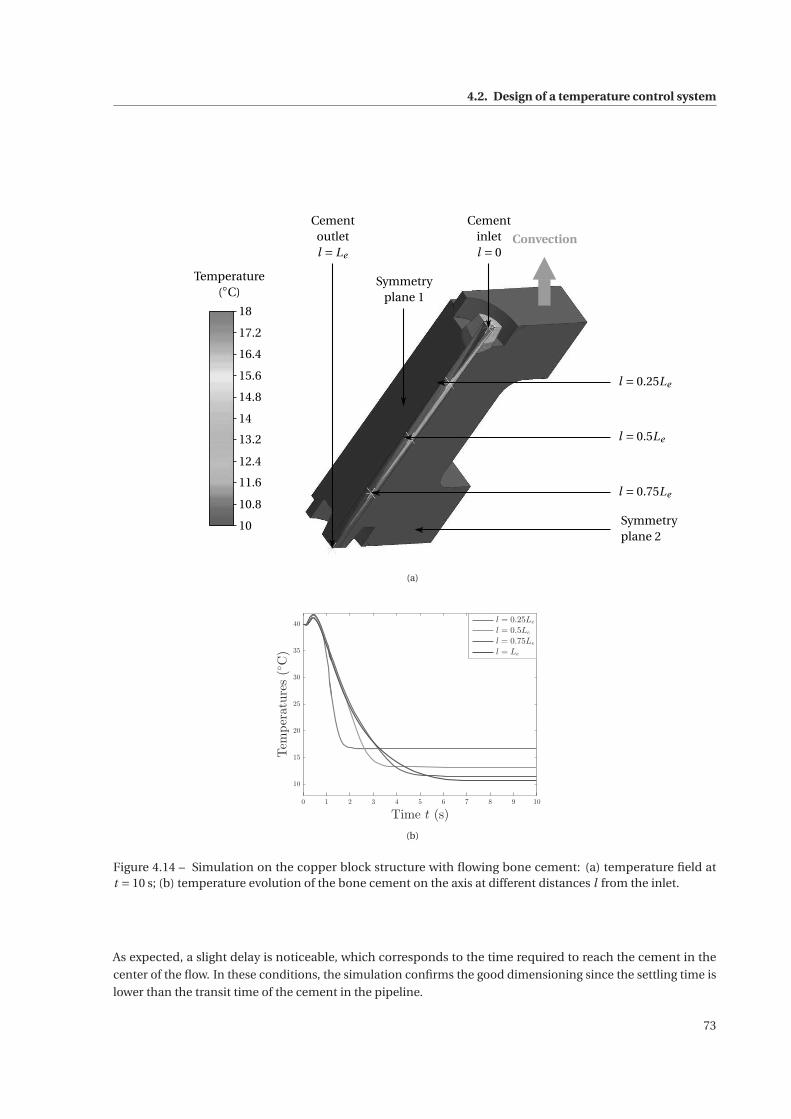
4.2. Design of a temperature control system
Convection
Symmetryplane 1
Cementoutletl = Le
l = 0.25Le
l = 0.5Le
l = 0.75Le
Symmetryplane 2
Cementinletl = 0
18
10
17.2
16.4
15.6
14.8
14
13.2
12.4
11.6
10.8
Temperature(◦C)
(a)
0 1 2 3 4 5 6 7 8 9 10
Time t (s)
10
15
20
25
30
35
40
Temperatures(◦C)
l = 0.25Le
l = 0.5Le
l = 0.75Le
l = Le
(b)
Figure 4.14 – Simulation on the copper block structure with flowing bone cement: (a) temperature field att = 10 s; (b) temperature evolution of the bone cement on the axis at different distances l from the inlet.
As expected, a slight delay is noticeable, which corresponds to the time required to reach the cement in the
center of the flow. In these conditions, the simulation confirms the good dimensioning since the settling time is
lower than the transit time of the cement in the pipeline.
73
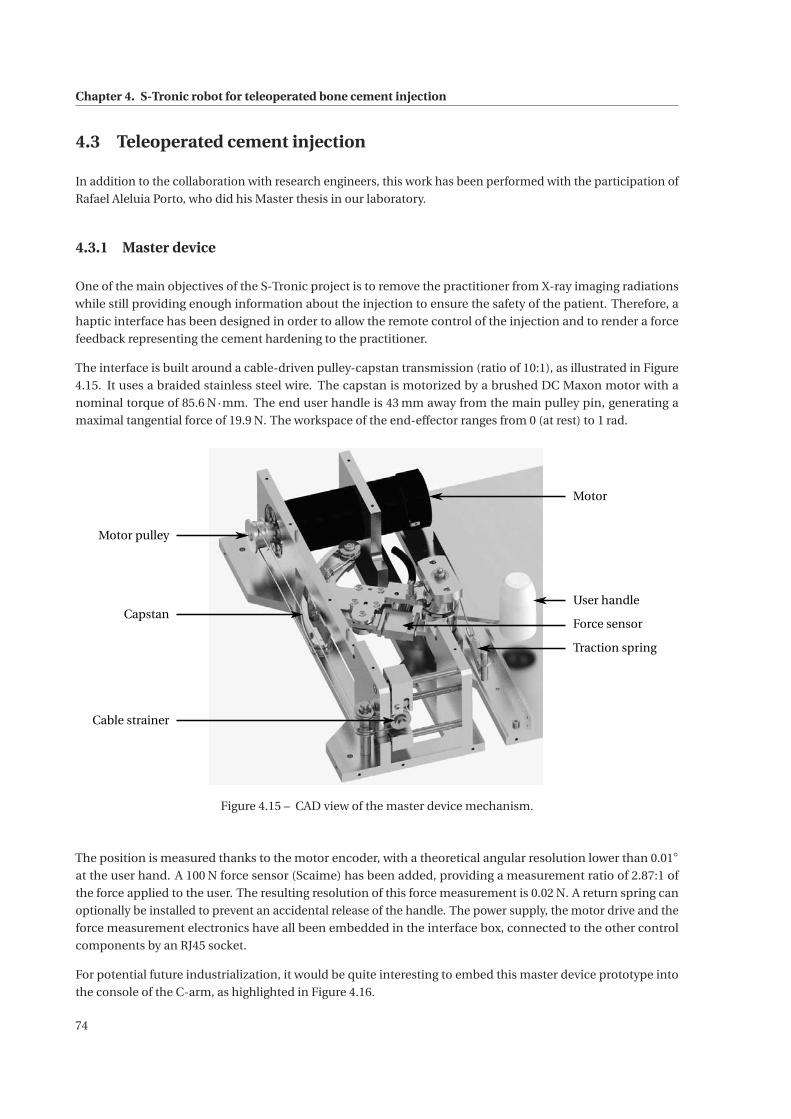
Chapter 4. S-Tronic robot for teleoperated bone cement injection
4.3 Teleoperated cement injection
In addition to the collaboration with research engineers, this work has been performed with the participation of
Rafael Aleluia Porto, who did his Master thesis in our laboratory.
4.3.1 Master device
One of the main objectives of the S-Tronic project is to remove the practitioner from X-ray imaging radiations
while still providing enough information about the injection to ensure the safety of the patient. Therefore, a
haptic interface has been designed in order to allow the remote control of the injection and to render a force
feedback representing the cement hardening to the practitioner.
The interface is built around a cable-driven pulley-capstan transmission (ratio of 10:1), as illustrated in Figure
4.15. It uses a braided stainless steel wire. The capstan is motorized by a brushed DC Maxon motor with a
nominal torque of 85.6 N·mm. The end user handle is 43 mm away from the main pulley pin, generating a
maximal tangential force of 19.9 N. The workspace of the end-effector ranges from 0 (at rest) to 1 rad.
Motor
User handle
Force sensor
Traction spring
Motor pulley
Capstan
Cable strainer
Figure 4.15 – CAD view of the master device mechanism.
The position is measured thanks to the motor encoder, with a theoretical angular resolution lower than 0.01◦
at the user hand. A 100 N force sensor (Scaime) has been added, providing a measurement ratio of 2.87:1 of
the force applied to the user. The resulting resolution of this force measurement is 0.02 N. A return spring can
optionally be installed to prevent an accidental release of the handle. The power supply, the motor drive and the
force measurement electronics have all been embedded in the interface box, connected to the other control
components by an RJ45 socket.
For potential future industrialization, it would be quite interesting to embed this master device prototype into
the console of the C-arm, as highlighted in Figure 4.16.
74
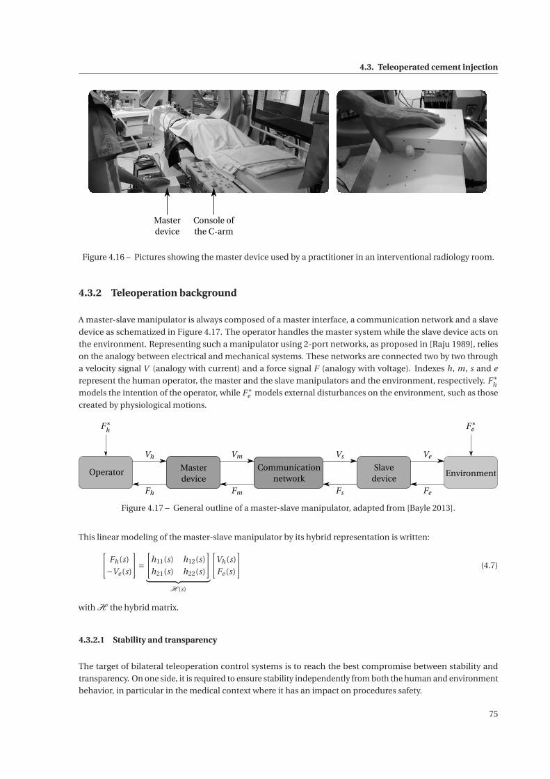
4.3. Teleoperated cement injection
Masterdevice
Console ofthe C-arm
Figure 4.16 – Pictures showing the master device used by a practitioner in an interventional radiology room.
4.3.2 Teleoperation background
A master-slave manipulator is always composed of a master interface, a communication network and a slave
device as schematized in Figure 4.17. The operator handles the master system while the slave device acts on
the environment. Representing such a manipulator using 2-port networks, as proposed in [Raju 1989], relies
on the analogy between electrical and mechanical systems. These networks are connected two by two through
a velocity signal V (analogy with current) and a force signal F (analogy with voltage). Indexes h, m, s and e
represent the human operator, the master and the slave manipulators and the environment, respectively. F∗h
models the intention of the operator, while F∗e models external disturbances on the environment, such as those
created by physiological motions.
Vh Vm Vs Ve
FeFsFmFh
Operator Masterdevice
Communicationnetwork
Slavedevice
Environment
F∗eF∗
h
Figure 4.17 – General outline of a master-slave manipulator, adapted from [Bayle 2013].
This linear modeling of the master-slave manipulator by its hybrid representation is written:[Fh(s)
−Ve (s)
]=[
h11(s) h12(s)
h21(s) h22(s)
]︸ ︷︷ ︸
H (s)
[Vh(s)
Fe (s)
](4.7)
with H the hybrid matrix.
4.3.2.1 Stability and transparency
The target of bilateral teleoperation control systems is to reach the best compromise between stability and
transparency. On one side, it is required to ensure stability independently from both the human and environment
behavior, in particular in the medical context where it has an impact on procedures safety.
75
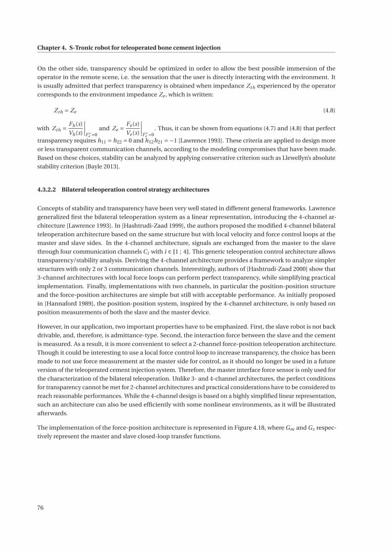
Chapter 4. S-Tronic robot for teleoperated bone cement injection
On the other side, transparency should be optimized in order to allow the best possible immersion of the
operator in the remote scene, i.e. the sensation that the user is directly interacting with the environment. It
is usually admitted that perfect transparency is obtained when impedance Zth experienced by the operator
corresponds to the environment impedance Ze , which is written:
Zth = Ze (4.8)
with Zth = Fh(s)
Vh(s)
∣∣∣∣F∗
e =0and Ze =
Fe (s)
Ve (s)
∣∣∣∣F∗
e =0. Thus, it can be shown from equations (4.7) and (4.8) that perfect
transparency requires h11 = h22 = 0 and h12h21 =−1 [Lawrence 1993]. These criteria are applied to design more
or less transparent communication channels, according to the modeling compromises that have been made.
Based on these choices, stability can be analyzed by applying conservative criterion such as Llewellyn’s absolute
stability criterion [Bayle 2013].
4.3.2.2 Bilateral teleoperation control strategy architectures
Concepts of stability and transparency have been very well stated in different general frameworks. Lawrence
generalized first the bilateral teleoperation system as a linear representation, introducing the 4-channel ar-
chitecture [Lawrence 1993]. In [Hashtrudi-Zaad 1999], the authors proposed the modified 4-channel bilateral
teleoperation architecture based on the same structure but with local velocity and force control loops at the
master and slave sides. In the 4-channel architecture, signals are exchanged from the master to the slave
through four communication channels Ci with i ∈ �1 ; 4 . This generic teleoperation control architecture allows
transparency/stability analysis. Deriving the 4-channel architecture provides a framework to analyze simpler
structures with only 2 or 3 communication channels. Interestingly, authors of [Hashtrudi-Zaad 2000] show that
3-channel architectures with local force loops can perform perfect transparency, while simplifying practical
implementation. Finally, implementations with two channels, in particular the position-position structure
and the force-position architectures are simple but still with acceptable performance. As initially proposed
in [Hannaford 1989], the position-position system, inspired by the 4-channel architecture, is only based on
position measurements of both the slave and the master device.
However, in our application, two important properties have to be emphasized. First, the slave robot is not back
drivable, and, therefore, is admittance-type. Second, the interaction force between the slave and the cement
is measured. As a result, it is more convenient to select a 2-channel force-position teleoperation architecture.
Though it could be interesting to use a local force control loop to increase transparency, the choice has been
made to not use force measurement at the master side for control, as it should no longer be used in a future
version of the teleoperated cement injection system. Therefore, the master interface force sensor is only used for
the characterization of the bilateral teleoperation. Unlike 3- and 4-channel architectures, the perfect conditions
for transparency cannot be met for 2-channel architectures and practical considerations have to be considered to
reach reasonable performances. While the 4-channel design is based on a highly simplified linear representation,
such an architecture can also be used efficiently with some nonlinear environments, as it will be illustrated
afterwards.
The implementation of the force-position architecture is represented in Figure 4.18, where Gm and Gs respec-
tively represent the master and slave closed-loop transfer functions.
76
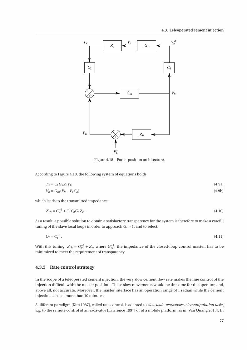
4.3. Teleoperated cement injection
Ve
Vh
F∗h
Fh
+−
+−
FeZe Gs
C2 C1
Gm
Zh
V de
Figure 4.18 – Force-position architecture.
According to Figure 4.18, the following system of equations holds:
Fe =C1Gs ZeVh (4.9a)
Vh =Gm(Fh −FeC2) (4.9b)
which leads to the transmitted impedance:
Zth =G−1m +C1C2Gs Ze . (4.10)
As a result, a possible solution to obtain a satisfactory transparency for the system is therefore to make a careful
tuning of the slave local loops in order to approach Gs ≈ 1, and to select:
C2 =C−11 . (4.11)
With this tuning, Zth = G−1m + Ze , where G−1
m , the impedance of the closed-loop control master, has to be
minimized to meet the requirement of transparency.
4.3.3 Rate control strategy
In the scope of a teleoperated cement injection, the very slow cement flow rate makes the fine control of the
injection difficult with the master position. These slow movements would be tiresome for the operator, and,
above all, not accurate. Moreover, the master interface has an operation range of 1 radian while the cement
injection can last more than 10 minutes.
A different paradigm [Kim 1987], called rate control, is adapted to slow wide-workspace telemanipulation tasks,
e.g. to the remote control of an excavator [Lawrence 1997] or of a mobile platform, as in [Van Quang 2013]. In
77
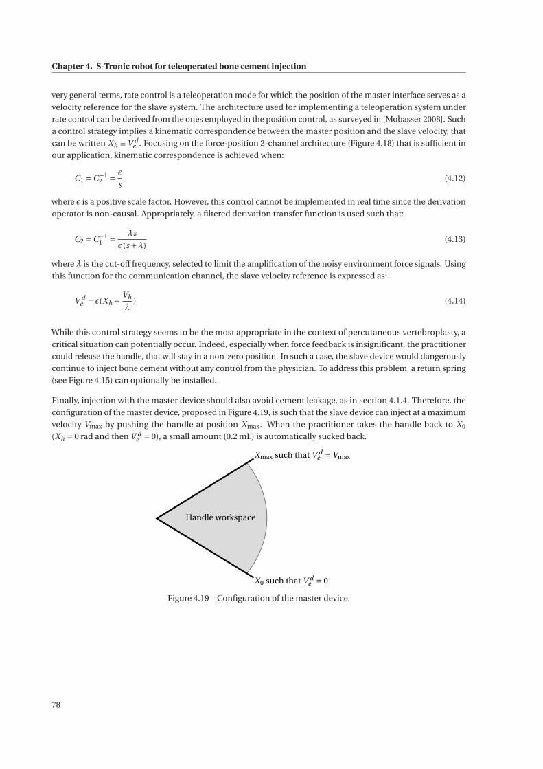
Chapter 4. S-Tronic robot for teleoperated bone cement injection
very general terms, rate control is a teleoperation mode for which the position of the master interface serves as a
velocity reference for the slave system. The architecture used for implementing a teleoperation system under
rate control can be derived from the ones employed in the position control, as surveyed in [Mobasser 2008]. Such
a control strategy implies a kinematic correspondence between the master position and the slave velocity, that
can be written Xh ≡V de . Focusing on the force-position 2-channel architecture (Figure 4.18) that is sufficient in
our application, kinematic correspondence is achieved when:
C1 =C−12 = ε
s(4.12)
where ε is a positive scale factor. However, this control cannot be implemented in real time since the derivation
operator is non-causal. Appropriately, a filtered derivation transfer function is used such that:
C2 =C−11 = λs
ε (s +λ)(4.13)
where λ is the cut-off frequency, selected to limit the amplification of the noisy environment force signals. Using
this function for the communication channel, the slave velocity reference is expressed as:
V de = ε(Xh + Vh
λ) (4.14)
While this control strategy seems to be the most appropriate in the context of percutaneous vertebroplasty, a
critical situation can potentially occur. Indeed, especially when force feedback is insignificant, the practitioner
could release the handle, that will stay in a non-zero position. In such a case, the slave device would dangerously
continue to inject bone cement without any control from the physician. To address this problem, a return spring
(see Figure 4.15) can optionally be installed.
Finally, injection with the master device should also avoid cement leakage, as in section 4.1.4. Therefore, the
configuration of the master device, proposed in Figure 4.19, is such that the slave device can inject at a maximum
velocity Vmax by pushing the handle at position Xmax. When the practitioner takes the handle back to X0
(Xh = 0 rad and then V de = 0), a small amount (0.2 mL) is automatically sucked back.
Handle workspace
X0 such that V de = 0
Xmax such that V de =Vmax
Figure 4.19 – Configuration of the master device.
78
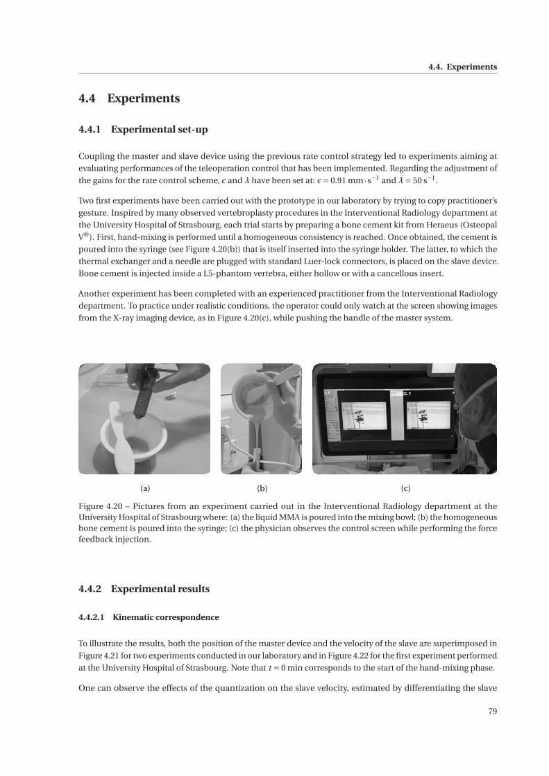
4.4. Experiments
4.4 Experiments
4.4.1 Experimental set-up
Coupling the master and slave device using the previous rate control strategy led to experiments aiming at
evaluating performances of the teleoperation control that has been implemented. Regarding the adjustment of
the gains for the rate control scheme, ε and λ have been set at: ε= 0.91 mm·s−1 and λ= 50 s−1.
Two first experiments have been carried out with the prototype in our laboratory by trying to copy practitioner’s
gesture. Inspired by many observed vertebroplasty procedures in the Interventional Radiology department at
the University Hospital of Strasbourg, each trial starts by preparing a bone cement kit from Heraeus (Osteopal
V®). First, hand-mixing is performed until a homogeneous consistency is reached. Once obtained, the cement is
poured into the syringe (see Figure 4.20(b)) that is itself inserted into the syringe holder. The latter, to which the
thermal exchanger and a needle are plugged with standard Luer-lock connectors, is placed on the slave device.
Bone cement is injected inside a L5-phantom vertebra, either hollow or with a cancellous insert.
Another experiment has been completed with an experienced practitioner from the Interventional Radiology
department. To practice under realistic conditions, the operator could only watch at the screen showing images
from the X-ray imaging device, as in Figure 4.20(c), while pushing the handle of the master system.
(a) (c)(b)
Figure 4.20 – Pictures from an experiment carried out in the Interventional Radiology department at theUniversity Hospital of Strasbourg where: (a) the liquid MMA is poured into the mixing bowl; (b) the homogeneousbone cement is poured into the syringe; (c) the physician observes the control screen while performing the forcefeedback injection.
4.4.2 Experimental results
4.4.2.1 Kinematic correspondence
To illustrate the results, both the position of the master device and the velocity of the slave are superimposed in
Figure 4.21 for two experiments conducted in our laboratory and in Figure 4.22 for the first experiment performed
at the University Hospital of Strasbourg. Note that t = 0 min corresponds to the start of the hand-mixing phase.
One can observe the effects of the quantization on the slave velocity, estimated by differentiating the slave
79
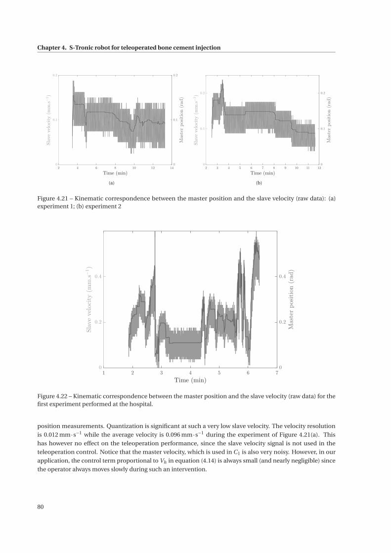
Chapter 4. S-Tronic robot for teleoperated bone cement injection
2 4 6 8 10 12 14
Time (min)
0
0.1
0.2
Slavevelocity(mm.s−1)
0
0.1
0.2
Masterposition(rad)
(a)
2 3 4 5 6 7 8 9 10 11 12
Time (min)
0
0.1
0.2
Slavevelocity(mm.s−1)
0
0.1
0.2
Masterposition(rad)
(b)
Figure 4.21 – Kinematic correspondence between the master position and the slave velocity (raw data): (a)experiment 1; (b) experiment 2
1 2 3 4 5 6 7
Time (min)
0
0.2
0.4
Slavevelocity(mm.s−1)
0
0.2
0.4
Masterposition(rad)
Figure 4.22 – Kinematic correspondence between the master position and the slave velocity (raw data) for thefirst experiment performed at the hospital.
position measurements. Quantization is significant at such a very low slave velocity. The velocity resolution
is 0.012 mm·s−1 while the average velocity is 0.096 mm·s−1 during the experiment of Figure 4.21(a). This
has however no effect on the teleoperation performance, since the slave velocity signal is not used in the
teleoperation control. Notice that the master velocity, which is used in C1 is also very noisy. However, in our
application, the control term proportional to Vh in equation (4.14) is always small (and nearly negligible) since
the operator always moves slowly during such an intervention.
80
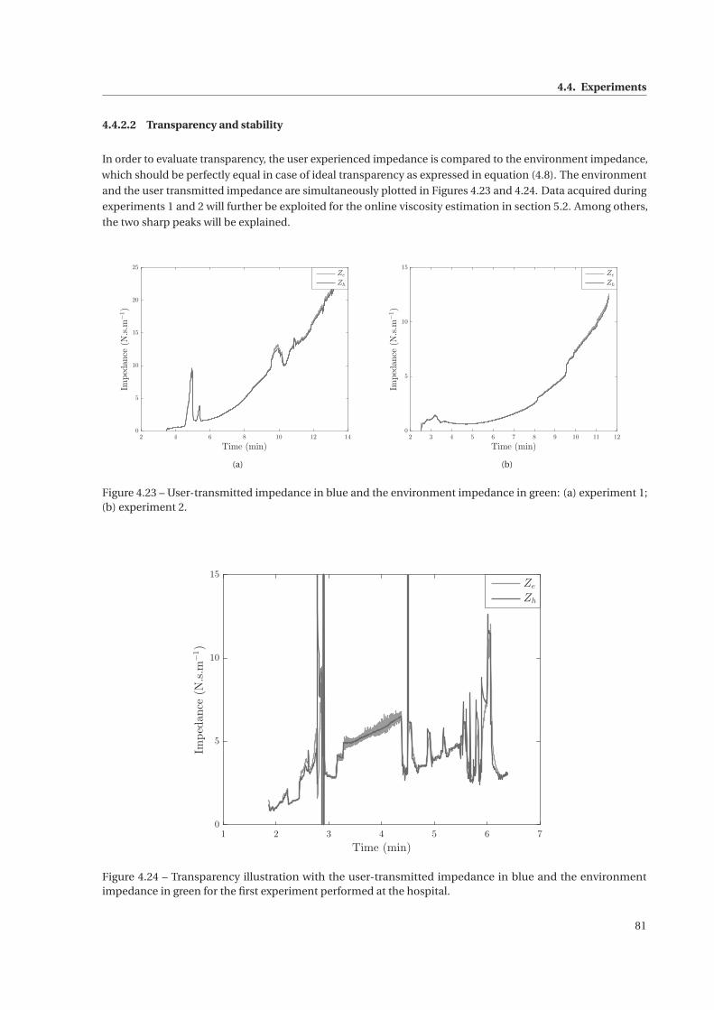
4.4. Experiments
4.4.2.2 Transparency and stability
In order to evaluate transparency, the user experienced impedance is compared to the environment impedance,
which should be perfectly equal in case of ideal transparency as expressed in equation (4.8). The environment
and the user transmitted impedance are simultaneously plotted in Figures 4.23 and 4.24. Data acquired during
experiments 1 and 2 will further be exploited for the online viscosity estimation in section 5.2. Among others,
the two sharp peaks will be explained.
2 4 6 8 10 12 14
Time (min)
0
5
10
15
20
25
Impedance(N.s.m
−1)
Ze
Zh
(a)
2 3 4 5 6 7 8 9 10 11 12
Time (min)
0
5
10
15
Impedance(N.s.m
−1)
Ze
Zh
(b)
Figure 4.23 – User-transmitted impedance in blue and the environment impedance in green: (a) experiment 1;(b) experiment 2.
1 2 3 4 5 6 7
Time (min)
0
5
10
15
Impedance(N.s.m
−1)
Ze
Zh
Figure 4.24 – Transparency illustration with the user-transmitted impedance in blue and the environmentimpedance in green for the first experiment performed at the hospital.
81
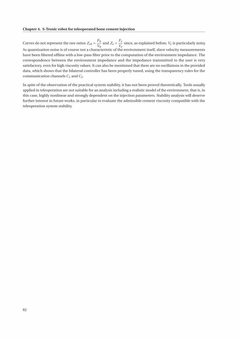
Chapter 4. S-Tronic robot for teleoperated bone cement injection
Curves do not represent the raw ratios Zth = Fh
Vhand Ze =
Fe
Vesince, as explained before, Ve is particularly noisy.
As quantization noise is of course not a characteristic of the environment itself, slave velocity measurements
have been filtered offline with a low-pass filter prior to the computation of the environment impedance. The
correspondence between the environment impedance and the impedance transmitted to the user is very
satisfactory, even for high viscosity values. It can also be mentioned that there are no oscillations in the provided
data, which shows that the bilateral controller has been properly tuned, using the transparency rules for the
communication channels C1 and C2.
In spite of the observation of the practical system stability, it has not been proved theoretically. Tools usually
applied in teleoperation are not suitable for an analysis including a realistic model of the environment, that is, in
this case, highly nonlinear and strongly dependent on the injection parameters. Stability analysis will deserve
further interest in future works, in particular to evaluate the admissible cement viscosity compatible with the
teleoperation system stability.
82
5 Online estimation and control of bonecement viscosity
Contents
5.1 Temperature control . . . . . . . . . . . . . . . . . . . . . . . . . . . . . . . . . . . . . . . . . . . . . . 84
5.1.1 Modeling and identification of the thermal block . . . . . . . . . . . . . . . . . . . . . . . . . 85
5.1.2 Temperature closed-loop control . . . . . . . . . . . . . . . . . . . . . . . . . . . . . . . . . . 90
5.1.3 Effect of temperature changes on the cement mechanical properties . . . . . . . . . . . . . 97
5.2 Viscosity estimation and control . . . . . . . . . . . . . . . . . . . . . . . . . . . . . . . . . . . . . . . 98
5.2.1 Online estimation of the bone cement viscosity . . . . . . . . . . . . . . . . . . . . . . . . . . 98
5.2.2 Viscosity control . . . . . . . . . . . . . . . . . . . . . . . . . . . . . . . . . . . . . . . . . . . . 103
83
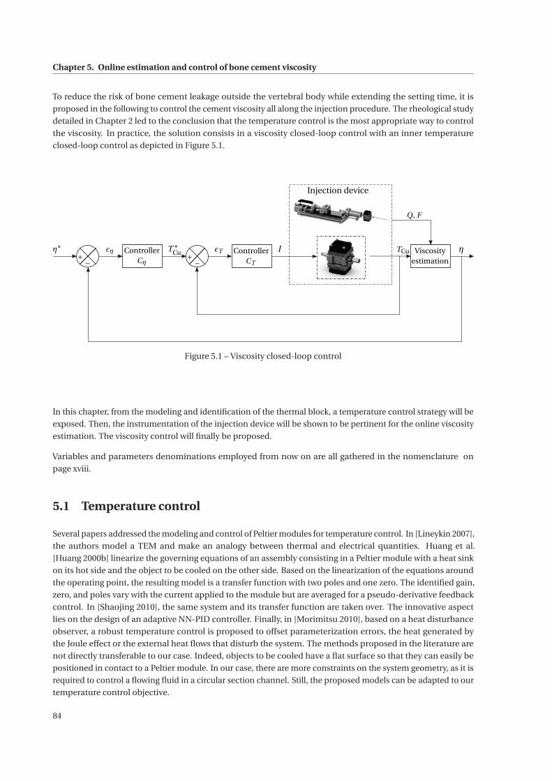
Chapter 5. Online estimation and control of bone cement viscosity
To reduce the risk of bone cement leakage outside the vertebral body while extending the setting time, it is
proposed in the following to control the cement viscosity all along the injection procedure. The rheological study
detailed in Chapter 2 led to the conclusion that the temperature control is the most appropriate way to control
the viscosity. In practice, the solution consists in a viscosity closed-loop control with an inner temperature
closed-loop control as depicted in Figure 5.1.
η∗+−
εη ControllerCη
T ∗Cu TCu Viscosity
estimation
Q, F
η+−
εT ControllerCT
I
Injection device
Figure 5.1 – Viscosity closed-loop control
In this chapter, from the modeling and identification of the thermal block, a temperature control strategy will be
exposed. Then, the instrumentation of the injection device will be shown to be pertinent for the online viscosity
estimation. The viscosity control will finally be proposed.
Variables and parameters denominations employed from now on are all gathered in the nomenclature on
page xviii.
5.1 Temperature control
Several papers addressed the modeling and control of Peltier modules for temperature control. In [Lineykin 2007],
the authors model a TEM and make an analogy between thermal and electrical quantities. Huang et al.
[Huang 2000b] linearize the governing equations of an assembly consisting in a Peltier module with a heat sink
on its hot side and the object to be cooled on the other side. Based on the linearization of the equations around
the operating point, the resulting model is a transfer function with two poles and one zero. The identified gain,
zero, and poles vary with the current applied to the module but are averaged for a pseudo-derivative feedback
control. In [Shaojing 2010], the same system and its transfer function are taken over. The innovative aspect
lies on the design of an adaptive NN-PID controller. Finally, in [Morimitsu 2010], based on a heat disturbance
observer, a robust temperature control is proposed to offset parameterization errors, the heat generated by
the Joule effect or the external heat flows that disturb the system. The methods proposed in the literature are
not directly transferable to our case. Indeed, objects to be cooled have a flat surface so that they can easily be
positioned in contact to a Peltier module. In our case, there are more constraints on the system geometry, as it is
required to control a flowing fluid in a circular section channel. Still, the proposed models can be adapted to our
temperature control objective.
84
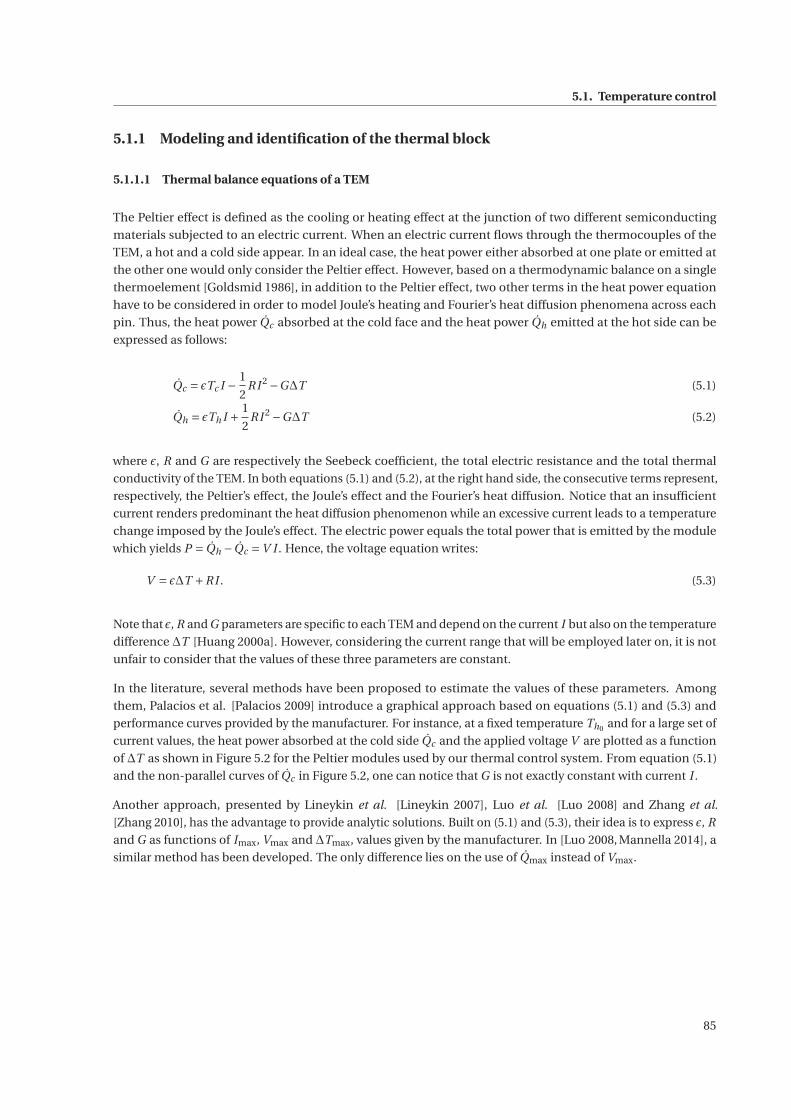
5.1. Temperature control
5.1.1 Modeling and identification of the thermal block
5.1.1.1 Thermal balance equations of a TEM
The Peltier effect is defined as the cooling or heating effect at the junction of two different semiconducting
materials subjected to an electric current. When an electric current flows through the thermocouples of the
TEM, a hot and a cold side appear. In an ideal case, the heat power either absorbed at one plate or emitted at
the other one would only consider the Peltier effect. However, based on a thermodynamic balance on a single
thermoelement [Goldsmid 1986], in addition to the Peltier effect, two other terms in the heat power equation
have to be considered in order to model Joule’s heating and Fourier’s heat diffusion phenomena across each
pin. Thus, the heat power Qc absorbed at the cold face and the heat power Qh emitted at the hot side can be
expressed as follows:
Qc = εTc I − 1
2RI 2 −GΔT (5.1)
Qh = εTh I + 1
2RI 2 −GΔT (5.2)
where ε, R and G are respectively the Seebeck coefficient, the total electric resistance and the total thermal
conductivity of the TEM. In both equations (5.1) and (5.2), at the right hand side, the consecutive terms represent,
respectively, the Peltier’s effect, the Joule’s effect and the Fourier’s heat diffusion. Notice that an insufficient
current renders predominant the heat diffusion phenomenon while an excessive current leads to a temperature
change imposed by the Joule’s effect. The electric power equals the total power that is emitted by the module
which yields P = Qh −Qc =V I . Hence, the voltage equation writes:
V = εΔT +RI . (5.3)
Note that ε, R and G parameters are specific to each TEM and depend on the current I but also on the temperature
difference ΔT [Huang 2000a]. However, considering the current range that will be employed later on, it is not
unfair to consider that the values of these three parameters are constant.
In the literature, several methods have been proposed to estimate the values of these parameters. Among
them, Palacios et al. [Palacios 2009] introduce a graphical approach based on equations (5.1) and (5.3) and
performance curves provided by the manufacturer. For instance, at a fixed temperature Th0 and for a large set of
current values, the heat power absorbed at the cold side Qc and the applied voltage V are plotted as a function
of ΔT as shown in Figure 5.2 for the Peltier modules used by our thermal control system. From equation (5.1)
and the non-parallel curves of Qc in Figure 5.2, one can notice that G is not exactly constant with current I .
Another approach, presented by Lineykin et al. [Lineykin 2007], Luo et al. [Luo 2008] and Zhang et al.
[Zhang 2010], has the advantage to provide analytic solutions. Built on (5.1) and (5.3), their idea is to express ε, R
and G as functions of Imax, Vmax and ΔTmax, values given by the manufacturer. In [Luo 2008, Mannella 2014], a
similar method has been developed. The only difference lies on the use of Qmax instead of Vmax.
85
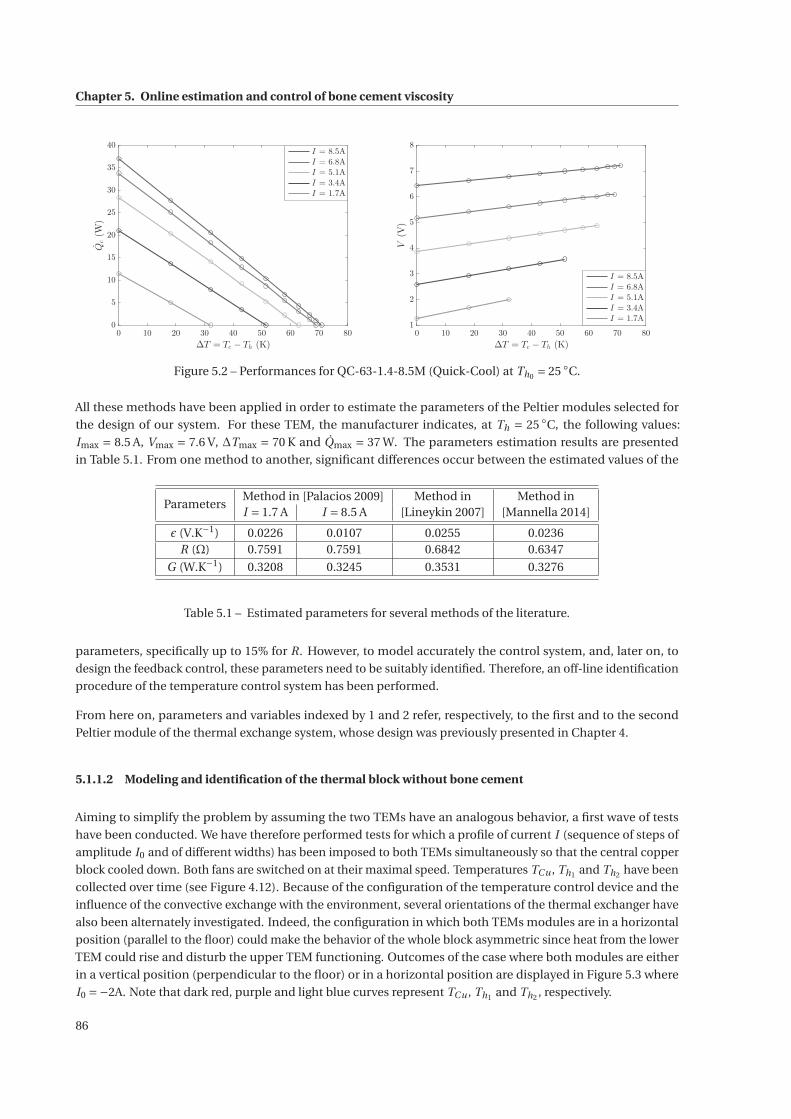
Chapter 5. Online estimation and control of bone cement viscosity
0 10 20 30 40 50 60 70 80
ΔT = Tc − Th (K)
0
5
10
15
20
25
30
35
40
Qc(W
)
I = 8.5A
I = 6.8A
I = 5.1A
I = 3.4A
I = 1.7A
0 10 20 30 40 50 60 70 80
ΔT = Tc − Th (K)
1
2
3
4
5
6
7
8
V(V)
I = 8.5A
I = 6.8A
I = 5.1A
I = 3.4A
I = 1.7A
Figure 5.2 – Performances for QC-63-1.4-8.5M (Quick-Cool) at Th0 = 25 ◦C.
All these methods have been applied in order to estimate the parameters of the Peltier modules selected for
the design of our system. For these TEM, the manufacturer indicates, at Th = 25 ◦C, the following values:
Imax = 8.5 A, Vmax = 7.6 V, ΔTmax = 70 K and Qmax = 37 W. The parameters estimation results are presented
in Table 5.1. From one method to another, significant differences occur between the estimated values of the
ParametersMethod in [Palacios 2009] Method in Method inI = 1.7 A I = 8.5 A [Lineykin 2007] [Mannella 2014]
ε (V.K−1) 0.0226 0.0107 0.0255 0.0236R (Ω) 0.7591 0.7591 0.6842 0.6347
G (W.K−1) 0.3208 0.3245 0.3531 0.3276
Table 5.1 – Estimated parameters for several methods of the literature.
parameters, specifically up to 15% for R. However, to model accurately the control system, and, later on, to
design the feedback control, these parameters need to be suitably identified. Therefore, an off-line identification
procedure of the temperature control system has been performed.
From here on, parameters and variables indexed by 1 and 2 refer, respectively, to the first and to the second
Peltier module of the thermal exchange system, whose design was previously presented in Chapter 4.
5.1.1.2 Modeling and identification of the thermal block without bone cement
Aiming to simplify the problem by assuming the two TEMs have an analogous behavior, a first wave of tests
have been conducted. We have therefore performed tests for which a profile of current I (sequence of steps of
amplitude I0 and of different widths) has been imposed to both TEMs simultaneously so that the central copper
block cooled down. Both fans are switched on at their maximal speed. Temperatures TCu , Th1 and Th2 have been
collected over time (see Figure 4.12). Because of the configuration of the temperature control device and the
influence of the convective exchange with the environment, several orientations of the thermal exchanger have
also been alternately investigated. Indeed, the configuration in which both TEMs modules are in a horizontal
position (parallel to the floor) could make the behavior of the whole block asymmetric since heat from the lower
TEM could rise and disturb the upper TEM functioning. Outcomes of the case where both modules are either
in a vertical position (perpendicular to the floor) or in a horizontal position are displayed in Figure 5.3 where
I0 =−2A. Note that dark red, purple and light blue curves represent TCu , Th1 and Th2 , respectively.
86
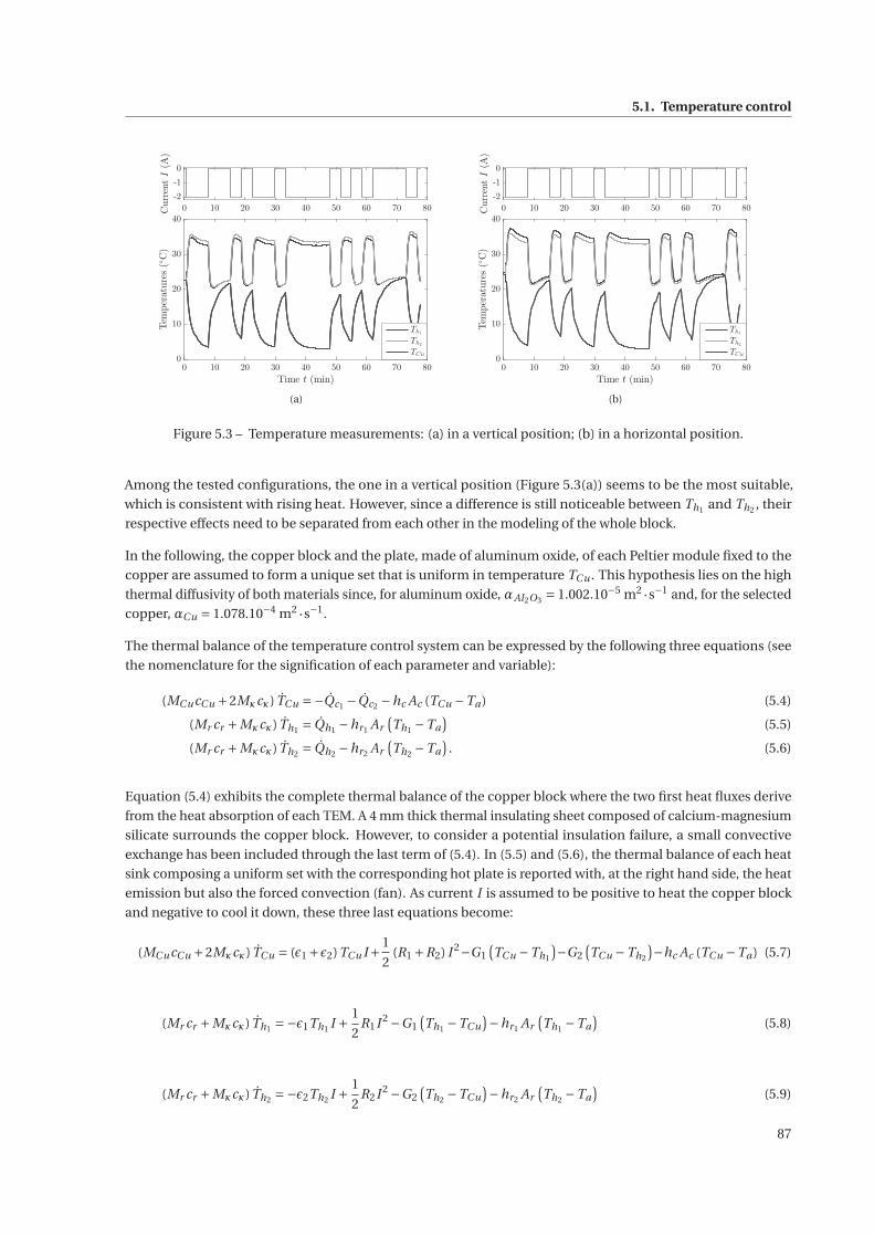
5.1. Temperature control
0 10 20 30 40 50 60 70 80
-2
-1
0CurrentI(A)
0 10 20 30 40 50 60 70 80
Time t (min)
0
10
20
30
40
Temperatures(◦C)
Th1
Th2
TCu
(a)
0 10 20 30 40 50 60 70 80
-2
-1
0
CurrentI(A)
0 10 20 30 40 50 60 70 80
Time t (min)
0
10
20
30
40
Temperatures(◦C)
Th1
Th2
TCu
(b)
Figure 5.3 – Temperature measurements: (a) in a vertical position; (b) in a horizontal position.
Among the tested configurations, the one in a vertical position (Figure 5.3(a)) seems to be the most suitable,
which is consistent with rising heat. However, since a difference is still noticeable between Th1 and Th2 , their
respective effects need to be separated from each other in the modeling of the whole block.
In the following, the copper block and the plate, made of aluminum oxide, of each Peltier module fixed to the
copper are assumed to form a unique set that is uniform in temperature TCu . This hypothesis lies on the high
thermal diffusivity of both materials since, for aluminum oxide, αAl2O3 = 1.002.10−5 m2 ·s−1 and, for the selected
copper, αCu = 1.078.10−4 m2 ·s−1.
The thermal balance of the temperature control system can be expressed by the following three equations (see
the nomenclature for the signification of each parameter and variable):
(MCucCu +2Mκcκ) TCu =−Qc1 −Qc2 −hc Ac (TCu −Ta) (5.4)
(Mr cr +Mκcκ) Th1 = Qh1 −hr1 Ar(Th1 −Ta
)(5.5)
(Mr cr +Mκcκ) Th2 = Qh2 −hr2 Ar(Th2 −Ta
). (5.6)
Equation (5.4) exhibits the complete thermal balance of the copper block where the two first heat fluxes derive
from the heat absorption of each TEM. A 4 mm thick thermal insulating sheet composed of calcium-magnesium
silicate surrounds the copper block. However, to consider a potential insulation failure, a small convective
exchange has been included through the last term of (5.4). In (5.5) and (5.6), the thermal balance of each heat
sink composing a uniform set with the corresponding hot plate is reported with, at the right hand side, the heat
emission but also the forced convection (fan). As current I is assumed to be positive to heat the copper block
and negative to cool it down, these three last equations become:
(MCucCu +2Mκcκ) TCu = (ε1 +ε2)TCu I+ 1
2(R1 +R2) I 2−G1
(TCu −Th1
)−G2
(TCu −Th2
)−hc Ac (TCu −Ta) (5.7)
(Mr cr +Mκcκ) Th1 =−ε1Th1 I + 1
2R1I 2 −G1
(Th1 −TCu
)−hr1 Ar
(Th1 −Ta
)(5.8)
(Mr cr +Mκcκ) Th2 =−ε2Th2 I + 1
2R2I 2 −G2
(Th2 −TCu
)−hr2 Ar
(Th2 −Ta
)(5.9)
87
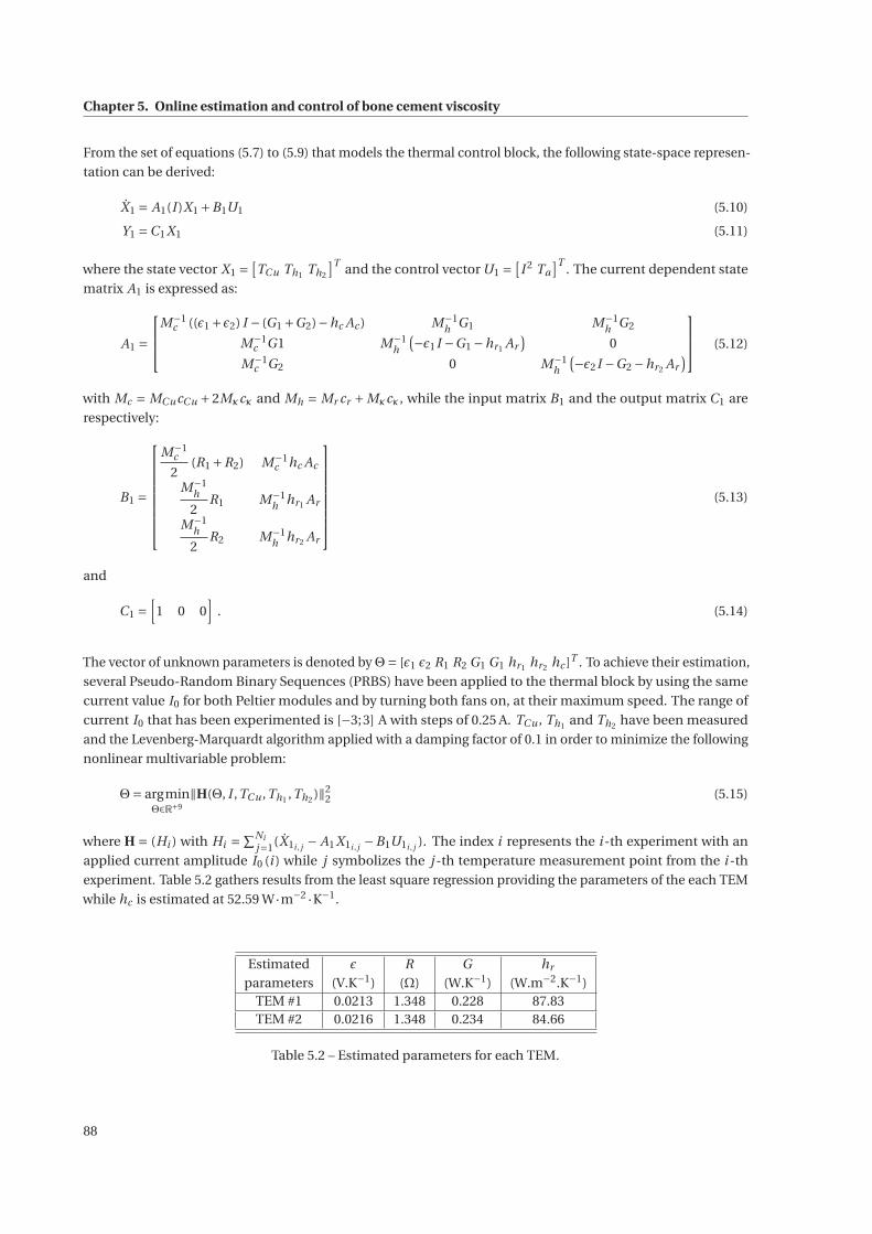
Chapter 5. Online estimation and control of bone cement viscosity
From the set of equations (5.7) to (5.9) that models the thermal control block, the following state-space represen-
tation can be derived:
X1 = A1(I )X1 +B1U1 (5.10)
Y1 =C1X1 (5.11)
where the state vector X1 =[TCu Th1 Th2
]T and the control vector U1 =[I 2 Ta
]T. The current dependent state
matrix A1 is expressed as:
A1 =
⎡⎢⎣M−1
c ((ε1 +ε2) I − (G1 +G2)−hc Ac ) M−1h G1 M−1
h G2
M−1c G1 M−1
h
(−ε1I −G1 −hr1 Ar
)0
M−1c G2 0 M−1
h
(−ε2I −G2 −hr2 Ar
)⎤⎥⎦ (5.12)
with Mc = MCucCu +2Mκcκ and Mh = Mr cr +Mκcκ, while the input matrix B1 and the output matrix C1 are
respectively:
B1 =
⎡⎢⎢⎢⎢⎢⎢⎢⎣
M−1c
2(R1 +R2) M−1
c hc Ac
M−1h
2R1 M−1
h hr1 Ar
M−1h
2R2 M−1
h hr2 Ar
⎤⎥⎥⎥⎥⎥⎥⎥⎦
(5.13)
and
C1 =[
1 0 0]
. (5.14)
The vector of unknown parameters is denoted by Θ= [ε1 ε2 R1 R2 G1 G1 hr1 hr2 hc ]T . To achieve their estimation,
several Pseudo-Random Binary Sequences (PRBS) have been applied to the thermal block by using the same
current value I0 for both Peltier modules and by turning both fans on, at their maximum speed. The range of
current I0 that has been experimented is [−3;3] A with steps of 0.25 A. TCu , Th1 and Th2 have been measured
and the Levenberg-Marquardt algorithm applied with a damping factor of 0.1 in order to minimize the following
nonlinear multivariable problem:
Θ= argminΘ∈R+9
‖H(Θ, I ,TCu ,Th1 ,Th2 )‖22 (5.15)
where H = (Hi ) with Hi =∑Ni
j=1(X1i , j − A1X1i , j −B1U1i , j ). The index i represents the i -th experiment with an
applied current amplitude I0 (i ) while j symbolizes the j -th temperature measurement point from the i -th
experiment. Table 5.2 gathers results from the least square regression providing the parameters of the each TEM
while hc is estimated at 52.59 W·m−2 ·K−1.
Estimated ε R G hr
parameters (V.K−1) (Ω) (W.K−1) (W.m−2.K−1)TEM #1 0.0213 1.348 0.228 87.83TEM #2 0.0216 1.348 0.234 84.66
Table 5.2 – Estimated parameters for each TEM.
88
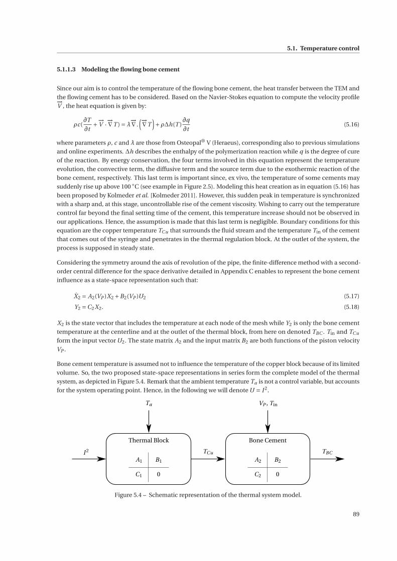
5.1. Temperature control
5.1.1.3 Modeling the flowing bone cement
Since our aim is to control the temperature of the flowing bone cement, the heat transfer between the TEM and
the flowing cement has to be considered. Based on the Navier-Stokes equation to compute the velocity profile−→V , the heat equation is given by:
ρc(∂T
∂t+−→
V ·−→∇T ) =λ
−→∇ .(−→∇T
)+ρΔh(T )
∂q
∂t(5.16)
where parameters ρ, c and λ are those from Osteopal® V (Heraeus), corresponding also to previous simulations
and online experiments. Δh describes the enthalpy of the polymerization reaction while q is the degree of cure
of the reaction. By energy conservation, the four terms involved in this equation represent the temperature
evolution, the convective term, the diffusive term and the source term due to the exothermic reaction of the
bone cement, respectively. This last term is important since, ex vivo, the temperature of some cements may
suddenly rise up above 100 ◦C (see example in Figure 2.5). Modeling this heat creation as in equation (5.16) has
been proposed by Kolmeder et al. [Kolmeder 2011]. However, this sudden peak in temperature is synchronized
with a sharp and, at this stage, uncontrollable rise of the cement viscosity. Wishing to carry out the temperature
control far beyond the final setting time of the cement, this temperature increase should not be observed in
our applications. Hence, the assumption is made that this last term is negligible. Boundary conditions for this
equation are the copper temperature TCu that surrounds the fluid stream and the temperature Tin of the cement
that comes out of the syringe and penetrates in the thermal regulation block. At the outlet of the system, the
process is supposed in steady state.
Considering the symmetry around the axis of revolution of the pipe, the finite-difference method with a second-
order central difference for the space derivative detailed in Appendix C enables to represent the bone cement
influence as a state-space representation such that:
X2 = A2(VP )X2 +B2(VP )U2 (5.17)
Y2 =C2X2. (5.18)
X2 is the state vector that includes the temperature at each node of the mesh while Y2 is only the bone cement
temperature at the centerline and at the outlet of the thermal block, from here on denoted TBC . Tin and TCu
form the input vector U2. The state matrix A2 and the input matrix B2 are both functions of the piston velocity
VP .
Bone cement temperature is assumed not to influence the temperature of the copper block because of its limited
volume. So, the two proposed state-space representations in series form the complete model of the thermal
system, as depicted in Figure 5.4. Remark that the ambient temperature Ta is not a control variable, but accounts
for the system operating point. Hence, in the following we will denote U = I 2.
Thermal Block Bone Cement
A1 B1
C1 0
A2 B2
C2 0
I 2 TCu TBC
VP , TinTa
Figure 5.4 – Schematic representation of the thermal system model.
89
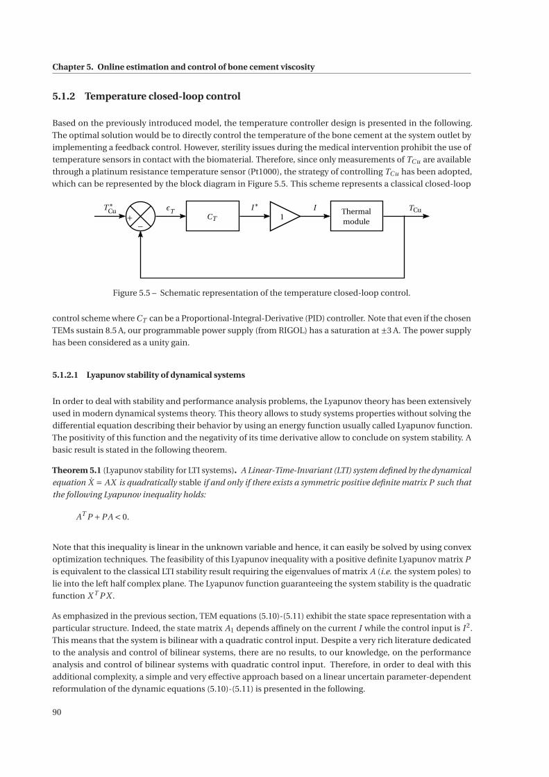
Chapter 5. Online estimation and control of bone cement viscosity
5.1.2 Temperature closed-loop control
Based on the previously introduced model, the temperature controller design is presented in the following.
The optimal solution would be to directly control the temperature of the bone cement at the system outlet by
implementing a feedback control. However, sterility issues during the medical intervention prohibit the use of
temperature sensors in contact with the biomaterial. Therefore, since only measurements of TCu are available
through a platinum resistance temperature sensor (Pt1000), the strategy of controlling TCu has been adopted,
which can be represented by the block diagram in Figure 5.5. This scheme represents a classical closed-loop
T∗Cu
+−
εTCT
I∗1
I Thermalmodule
TCu
Figure 5.5 – Schematic representation of the temperature closed-loop control.
control scheme where CT can be a Proportional-Integral-Derivative (PID) controller. Note that even if the chosen
TEMs sustain 8.5 A, our programmable power supply (from RIGOL) has a saturation at ±3 A. The power supply
has been considered as a unity gain.
5.1.2.1 Lyapunov stability of dynamical systems
In order to deal with stability and performance analysis problems, the Lyapunov theory has been extensively
used in modern dynamical systems theory. This theory allows to study systems properties without solving the
differential equation describing their behavior by using an energy function usually called Lyapunov function.
The positivity of this function and the negativity of its time derivative allow to conclude on system stability. A
basic result is stated in the following theorem.
Theorem 5.1 (Lyapunov stability for LTI systems). A Linear-Time-Invariant (LTI) system defined by the dynamical
equation X = AX is quadratically stable if and only if there exists a symmetric positive definite matrix P such that
the following Lyapunov inequality holds:
AT P +PA < 0.
Note that this inequality is linear in the unknown variable and hence, it can easily be solved by using convex
optimization techniques. The feasibility of this Lyapunov inequality with a positive definite Lyapunov matrix P
is equivalent to the classical LTI stability result requiring the eigenvalues of matrix A (i.e. the system poles) to
lie into the left half complex plane. The Lyapunov function guaranteeing the system stability is the quadratic
function X T P X .
As emphasized in the previous section, TEM equations (5.10)-(5.11) exhibit the state space representation with a
particular structure. Indeed, the state matrix A1 depends affinely on the current I while the control input is I 2.
This means that the system is bilinear with a quadratic control input. Despite a very rich literature dedicated
to the analysis and control of bilinear systems, there are no results, to our knowledge, on the performance
analysis and control of bilinear systems with quadratic control input. Therefore, in order to deal with this
additional complexity, a simple and very effective approach based on a linear uncertain parameter-dependent
reformulation of the dynamic equations (5.10)-(5.11) is presented in the following.
90
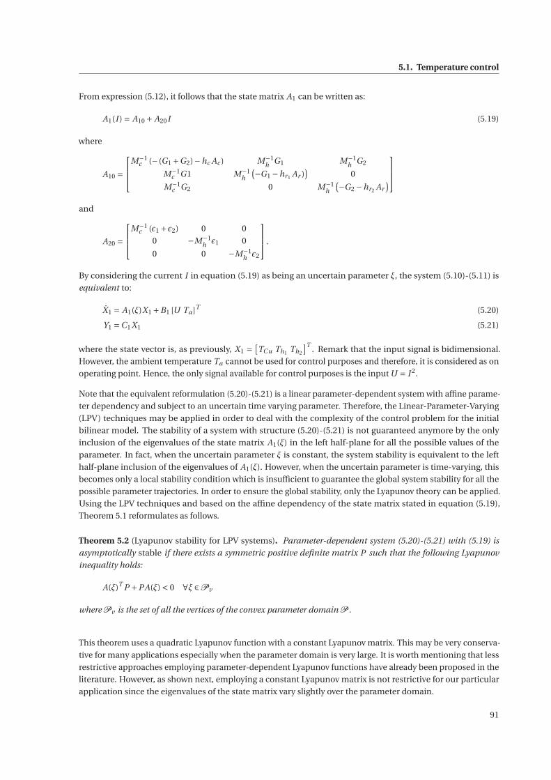
5.1. Temperature control
From expression (5.12), it follows that the state matrix A1 can be written as:
A1(I ) = A10 + A20I (5.19)
where
A10 =
⎡⎢⎣M−1
c (− (G1 +G2)−hc Ac ) M−1h G1 M−1
h G2
M−1c G1 M−1
h
(−G1 −hr1 Ar )
)0
M−1c G2 0 M−1
h
(−G2 −hr2 Ar
)⎤⎥⎦
and
A20 =
⎡⎢⎣M−1
c (ε1 +ε2) 0 0
0 −M−1h ε1 0
0 0 −M−1h ε2
⎤⎥⎦ .
By considering the current I in equation (5.19) as being an uncertain parameter ξ, the system (5.10)-(5.11) is
equivalent to:
X1 = A1(ξ)X1 +B1 [U Ta]T (5.20)
Y1 =C1X1 (5.21)
where the state vector is, as previously, X1 =[TCu Th1 Th2
]T . Remark that the input signal is bidimensional.
However, the ambient temperature Ta cannot be used for control purposes and therefore, it is considered as on
operating point. Hence, the only signal available for control purposes is the input U = I 2.
Note that the equivalent reformulation (5.20)-(5.21) is a linear parameter-dependent system with affine parame-
ter dependency and subject to an uncertain time varying parameter. Therefore, the Linear-Parameter-Varying
(LPV) techniques may be applied in order to deal with the complexity of the control problem for the initial
bilinear model. The stability of a system with structure (5.20)-(5.21) is not guaranteed anymore by the only
inclusion of the eigenvalues of the state matrix A1(ξ) in the left half-plane for all the possible values of the
parameter. In fact, when the uncertain parameter ξ is constant, the system stability is equivalent to the left
half-plane inclusion of the eigenvalues of A1(ξ). However, when the uncertain parameter is time-varying, this
becomes only a local stability condition which is insufficient to guarantee the global system stability for all the
possible parameter trajectories. In order to ensure the global stability, only the Lyapunov theory can be applied.
Using the LPV techniques and based on the affine dependency of the state matrix stated in equation (5.19),
Theorem 5.1 reformulates as follows.
Theorem 5.2 (Lyapunov stability for LPV systems). Parameter-dependent system (5.20)-(5.21) with (5.19) is
asymptotically stable if there exists a symmetric positive definite matrix P such that the following Lyapunov
inequality holds:
A(ξ)T P +PA(ξ) < 0 ∀ξ ∈Pv
where Pv is the set of all the vertices of the convex parameter domain P .
This theorem uses a quadratic Lyapunov function with a constant Lyapunov matrix. This may be very conserva-
tive for many applications especially when the parameter domain is very large. It is worth mentioning that less
restrictive approaches employing parameter-dependent Lyapunov functions have already been proposed in the
literature. However, as shown next, employing a constant Lyapunov matrix is not restrictive for our particular
application since the eigenvalues of the state matrix vary slightly over the parameter domain.
91
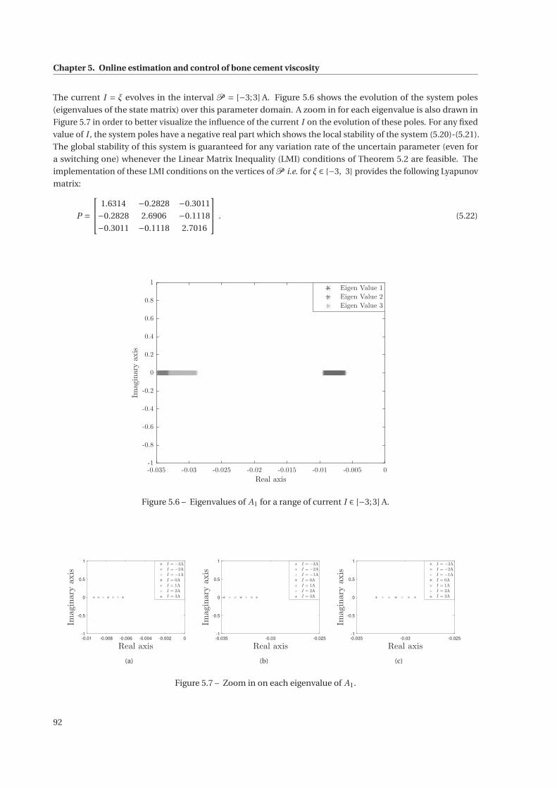
Chapter 5. Online estimation and control of bone cement viscosity
The current I = ξ evolves in the interval P = [−3;3] A. Figure 5.6 shows the evolution of the system poles
(eigenvalues of the state matrix) over this parameter domain. A zoom in for each eigenvalue is also drawn in
Figure 5.7 in order to better visualize the influence of the current I on the evolution of these poles. For any fixed
value of I , the system poles have a negative real part which shows the local stability of the system (5.20)-(5.21).
The global stability of this system is guaranteed for any variation rate of the uncertain parameter (even for
a switching one) whenever the Linear Matrix Inequality (LMI) conditions of Theorem 5.2 are feasible. The
implementation of these LMI conditions on the vertices of P i.e. for ξ ∈ {−3, 3} provides the following Lyapunov
matrix:
P =
⎡⎢⎣ 1.6314 −0.2828 −0.3011
−0.2828 2.6906 −0.1118
−0.3011 −0.1118 2.7016
⎤⎥⎦ . (5.22)
-0.035 -0.03 -0.025 -0.02 -0.015 -0.01 -0.005 0
Real axis
-1
-0.8
-0.6
-0.4
-0.2
0
0.2
0.4
0.6
0.8
1
Imaginaryaxis
Eigen Value 1
Eigen Value 2
Eigen Value 3
Figure 5.6 – Eigenvalues of A1 for a range of current I ∈ [−3;3] A.
-0.01 -0.008 -0.006 -0.004 -0.002 0
Real axis
-1
-0.5
0
0.5
1
Imaginaryaxis
I = −3A
I = −2A
I = −1A
I = 0A
I = 1A
I = 2A
I = 3A
(a)
-0.035 -0.03 -0.025
Real axis
-1
-0.5
0
0.5
1
Imaginaryaxis
I = −3A
I = −2A
I = −1A
I = 0A
I = 1A
I = 2A
I = 3A
(b)
-0.035 -0.03 -0.025
Real axis
-1
-0.5
0
0.5
1
Imaginaryaxis
I = −3A
I = −2A
I = −1A
I = 0A
I = 1A
I = 2A
I = 3A
(c)
Figure 5.7 – Zoom in on each eigenvalue of A1.
92
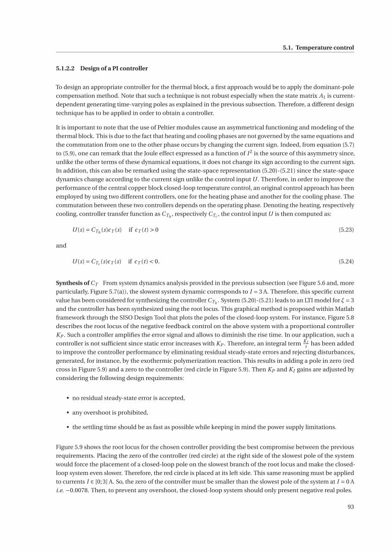
5.1. Temperature control
5.1.2.2 Design of a PI controller
To design an appropriate controller for the thermal block, a first approach would be to apply the dominant-pole
compensation method. Note that such a technique is not robust especially when the state matrix A1 is current-
dependent generating time-varying poles as explained in the previous subsection. Therefore, a different design
technique has to be applied in order to obtain a controller.
It is important to note that the use of Peltier modules cause an asymmetrical functioning and modeling of the
thermal block. This is due to the fact that heating and cooling phases are not governed by the same equations and
the commutation from one to the other phase occurs by changing the current sign. Indeed, from equation (5.7)
to (5.9), one can remark that the Joule effect expressed as a function of I 2 is the source of this asymmetry since,
unlike the other terms of these dynamical equations, it does not change its sign according to the current sign.
In addition, this can also be remarked using the state-space representation (5.20)-(5.21) since the state-space
dynamics change according to the current sign unlike the control input U . Therefore, in order to improve the
performance of the central copper block closed-loop temperature control, an original control approach has been
employed by using two different controllers, one for the heating phase and another for the cooling phase. The
commutation between these two controllers depends on the operating phase. Denoting the heating, respectively
cooling, controller transfer function as CTh , respectively CTc , the control input U is then computed as:
U (s) =CTh (s)εT (s) if εT (t ) > 0 (5.23)
and
U (s) =CTc (s)εT (s) if εT (t ) < 0. (5.24)
Synthesis of CT From system dynamics analysis provided in the previous subsection (see Figure 5.6 and, more
particularly, Figure 5.7(a)), the slowest system dynamic corresponds to I = 3 A. Therefore, this specific current
value has been considered for synthesizing the controller CTh . System (5.20)-(5.21) leads to an LTI model for ξ= 3
and the controller has been synthesized using the root locus. This graphical method is proposed within Matlab
framework through the SISO Design Tool that plots the poles of the closed-loop system. For instance, Figure 5.8
describes the root locus of the negative feedback control on the above system with a proportional controller
KP . Such a controller amplifies the error signal and allows to diminish the rise time. In our application, such a
controller is not sufficient since static error increases with KP . Therefore, an integral term KIs has been added
to improve the controller performance by eliminating residual steady-state errors and rejecting disturbances,
generated, for instance, by the exothermic polymerization reaction. This results in adding a pole in zero (red
cross in Figure 5.9) and a zero to the controller (red circle in Figure 5.9). Then KP and KI gains are adjusted by
considering the following design requirements:
• no residual steady-state error is accepted,
• any overshoot is prohibited,
• the settling time should be as fast as possible while keeping in mind the power supply limitations.
Figure 5.9 shows the root locus for the chosen controller providing the best compromise between the previous
requirements. Placing the zero of the controller (red circle) at the right side of the slowest pole of the system
would force the placement of a closed-loop pole on the slowest branch of the root locus and make the closed-
loop system even slower. Therefore, the red circle is placed at its left side. This same reasoning must be applied
to currents I ∈ [0;3] A. So, the zero of the controller must be smaller than the slowest pole of the system at I = 0 A
i.e. −0.0078. Then, to prevent any overshoot, the closed-loop system should only present negative real poles.
93
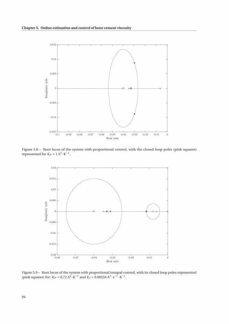
Chapter 5. Online estimation and control of bone cement viscosity
-0.1 -0.09 -0.08 -0.07 -0.06 -0.05 -0.04 -0.03 -0.02 -0.01 0
Real axis
-0.015
-0.01
-0.005
0
0.005
0.01
0.015Im
aginaryaxis
Figure 5.8 – Root locus of the system with proportional control, with the closed-loop poles (pink squares)represented for KP = 1 A2 ·K−1.
-0.06 -0.05 -0.04 -0.03 -0.02 -0.01 0
Real axis
-0.02
-0.015
-0.01
-0.005
0
0.005
0.01
0.015
0.02
Imaginaryaxis
Figure 5.9 – Root locus of the system with proportional integral control, with its closed loop poles represented(pink squares) for: KP = 0.72 A2 ·K−1 and KI = 0.00554 A2 ·s−1 ·K−1.
94
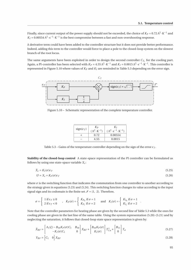
5.1. Temperature control
Finally, since current output of the power supply should not be exceeded, the choice of KP = 0.72 A2 ·K−1 and
KI = 0.00554 A2 ·s−1 ·K−1 is the best compromise between a fast and non-overshooting response.
A derivative term could have been added to the controller structure but it does not provide better performance.
Indeed, adding this term to the controller would force to place a pole to the closed-loop system on the slowest
branch of the root locus.
The same arguments have been exploited in order to design the second controller CTc for the cooling part.
Again, a PI-controller has been selected with KP = 4.55 A2 ·K−1 and KI = 0.0015 A2 ·s−1 ·K−1. This controller is
represented in Figure 5.10 where values of KP and KI are reminded in Table 5.3 depending on the error sign.
εT KP ++
KI1
s
sign(εT )×| . |
CT
I∗
Figure 5.10 – Schematic representation of the complete temperature controller.
sign(εT )KP KI
( A2 ·K−1) ( A2 ·s−1 ·K−1)+ 0.72 0.00554− 4.55 0.0015
Table 5.3 – Gains of the temperature controller depending on the sign of the error εT .
Stability of the closed-loop control A state-space representation of the PI controller can be formulated as
follows by using one state-space variable Xc :
Xc = KI (σ)εT (5.25)
U = Xc +KP (σ)εT (5.26)
where σ is the switching function that indicates the commutation from one controller to another according to
the strategy given in equations (5.23) and (5.24). This switching function changes its value according to the input
signal sign and its codomain is the finite set I = {1, 2}. Therefore,
σ={
1 if εT ≥ 0
2 if εT < 0, KP (σ) =
{KPh if σ= 1
KPc if σ= 2and KI (σ) =
{KIh if σ= 1
KIc if σ= 2.
Note that the controller parameters for heating phase are given by the second line of Table 5.3 while the ones for
cooling phase are given in the last line of the same table. Using the system representation (5.20)-(5.21) and by
neglecting the saturation, it follows that closed-loop state space representation is given by:
XBF =[
A1(ξ)−B10KP (σ)C1 B10
−KI (σ)C1 0
]XBF +
[B10KP (σ)
KI (σ)
]T ∗
Cu +[
B11
0
]Ta (5.27)
YBF =[C1 0
]XBF (5.28)
95
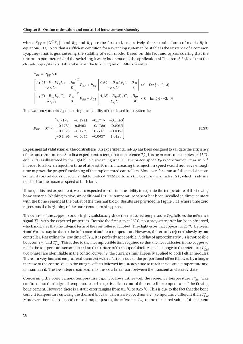
Chapter 5. Online estimation and control of bone cement viscosity
where XBF =[
X T1 Xc
]Tand B10 and B11 are the first and, respectively, the second column of matrix B1 in
equation(5.13). Note that a sufficient condition for a switching system to be stable is the existence of a common
Lyapunov matrix guaranteeing the stability of each mode. Based on this fact and by considering that the
uncertain parameter ξ and the switching law are independent, the application of Theorem 5.2 yields that the
closed-loop system is stable whenever the following set of LMIs is feasible:
PBF = P TBF > 0[
A1(ξ)−B10KPh C1 B10
−KIh C1 0
]T
PBF +PBF
[A1(ξ)−B10KPh C B10
−KIh C1 0
]< 0 for ξ ∈ {0, 3}
[A1(ξ)−B10KPc C1 B10
−KIc C1 0
]T
PBF +PBF
[A1(ξ)−B10KPc C1 B10
−KIc C1 0
]< 0 for ξ ∈ {−3, 0}
The Lyapunov matrix PBF ensuring the stability of the closed loop system is:
PBF = 103 ×
⎡⎢⎢⎢⎣
0.7178 −0.1731 −0.1775 −0.1490
−0.1731 0.5492 −0.1789 −0.0035
−0.1775 −0.1789 0.5507 −0.0057
−0.1490 −0.0035 −0.0057 1.0126
⎤⎥⎥⎥⎦ . (5.29)
Experimental validation of the controllers An experimental set-up has been designed to validate the efficiency
of the tuned controllers. As a first experiment, a temperature reference T ∗Cu has been constructed between 15 ◦C
and 30 ◦C as illustrated by the light blue curve in Figure 5.11. The piston speed VP is constant at 5 mm·min−1
in order to allow an injection time of at least 10 min. Increasing the injection speed would not leave enough
time to prove the proper functioning of the implemented controllers. Moreover, fans run at full speed since an
adjusted control does not seem suitable. Indeed, TEM performs the best for the smallest ΔT , which is always
reached for the maximal speed of both fans.
Through this first experiment, we also expected to confirm the ability to regulate the temperature of the flowing
bone cement. Working ex vivo, an additional Pt1000 temperature sensor has been installed in direct contact
with the bone cement at the outlet of the thermal block. Results are provided in Figure 5.11 where time zero
represents the beginning of the bone cement mixing phase.
The control of the copper block is highly satisfactory since the measured temperature TCu follows the reference
signal T ∗Cu with the expected properties. Despite the first step at 25 ◦C, no steady-state error has been observed,
which indicates that the integral term of the controller is adapted. The slight error that appears at 25 ◦C, between
4 and 6 min, may be due to the influence of ambient temperature. However, this error is rejected slowly by our
controller. Regarding the rise time of TCu , it is perfectly acceptable. A delay of approximately 5 s is noticeable
between TCu and T ∗Cu . This is due to the incompressible time required so that the heat diffusion in the copper to
reach the temperature sensor placed on the surface of the copper block. At each change in the reference T ∗Cu ,
two phases are identifiable in the control curve, i.e. the current simultaneously applied to both Peltier modules.
There is a very fast and emphasized transient (with a fast rise due to the proportional effect followed by a longer
increase of the control due to the integral effect) followed by a steady state to reach the desired temperature and
to maintain it. The low integral gain explains the slow linear part between the transient and steady state.
Concerning the bone cement temperature TBC , it follows rather well the reference temperature T ∗Cu . This
confirms that the designed temperature exchanger is able to control the centerline temperature of the flowing
bone cement. However, there is a static error ranging from 0.1 ◦C to 0.25 ◦C. This is due to the fact that the bone
cement temperature entering the thermal block at a non-zero speed has a Tin temperature different than T ∗Cu .
Moreover, there is no second control loop adjusting the reference T ∗Cu to the measured value of the cement
96
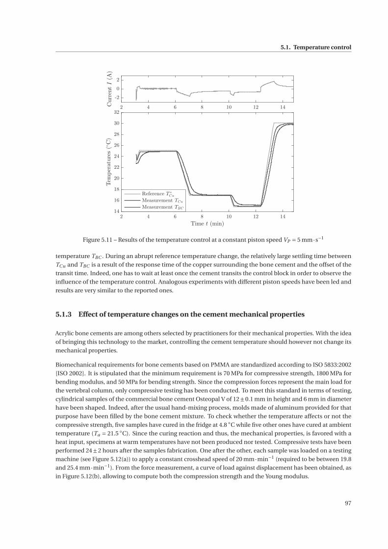
5.1. Temperature control
2 4 6 8 10 12 14
-2
0
2
CurrentI(A)
2 4 6 8 10 12 14
Time t (min)
14
16
18
20
22
24
26
28
30
32Temperatures(◦C)
Reference T∗
Cu
Measurement TCu
Measurement TBC
Figure 5.11 – Results of the temperature control at a constant piston speed VP = 5 mm·s−1
temperature TBC . During an abrupt reference temperature change, the relatively large settling time between
TCu and TBC is a result of the response time of the copper surrounding the bone cement and the offset of the
transit time. Indeed, one has to wait at least once the cement transits the control block in order to observe the
influence of the temperature control. Analogous experiments with different piston speeds have been led and
results are very similar to the reported ones.
5.1.3 Effect of temperature changes on the cement mechanical properties
Acrylic bone cements are among others selected by practitioners for their mechanical properties. With the idea
of bringing this technology to the market, controlling the cement temperature should however not change its
mechanical properties.
Biomechanical requirements for bone cements based on PMMA are standardized according to ISO 5833:2002
[ISO 2002]. It is stipulated that the minimum requirement is 70 MPa for compressive strength, 1800 MPa for
bending modulus, and 50 MPa for bending strength. Since the compression forces represent the main load for
the vertebral column, only compressive testing has been conducted. To meet this standard in terms of testing,
cylindrical samples of the commercial bone cement Osteopal V of 12±0.1 mm in height and 6 mm in diameter
have been shaped. Indeed, after the usual hand-mixing process, molds made of aluminum provided for that
purpose have been filled by the bone cement mixture. To check whether the temperature affects or not the
compressive strength, five samples have cured in the fridge at 4.8 ◦C while five other ones have cured at ambient
temperature (Ta = 21.5 ◦C). Since the curing reaction and thus, the mechanical properties, is favored with a
heat input, specimens at warm temperatures have not been produced nor tested. Compressive tests have been
performed 24±2 hours after the samples fabrication. One after the other, each sample was loaded on a testing
machine (see Figure 5.12(a)) to apply a constant crosshead speed of 20 mm·min−1 (required to be between 19.8
and 25.4 mm·min−1). From the force measurement, a curve of load against displacement has been obtained, as
in Figure 5.12(b), allowing to compute both the compression strength and the Young modulus.
97
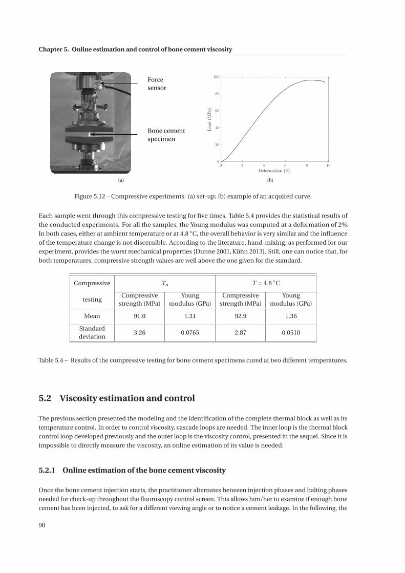
Chapter 5. Online estimation and control of bone cement viscosity
Forcesensor
Bone cementspecimen
(a)
0 2 4 6 8 10
Deformation (%)
0
20
40
60
80
100
Load(MPa)
(b)
Figure 5.12 – Compressive experiments: (a) set-up; (b) example of an acquired curve.
Each sample went through this compressive testing for five times. Table 5.4 provides the statistical results of
the conducted experiments. For all the samples, the Young modulus was computed at a deformation of 2%.
In both cases, either at ambient temperature or at 4.8 ◦C, the overall behavior is very similar and the influence
of the temperature change is not discernible. According to the literature, hand-mixing, as performed for our
experiment, provides the worst mechanical properties [Dunne 2001, Kühn 2013]. Still, one can notice that, for
both temperatures, compressive strength values are well above the one given for the standard.
Compressive Ta T = 4.8 ◦C
testingCompressive Young Compressive Young
strength (MPa) modulus (GPa) strength (MPa) modulus (GPa)
Mean 91.0 1.31 92.9 1.36
Standard3.26 0.0765 2.87 0.0510
deviation
Table 5.4 – Results of the compressive testing for bone cement specimens cured at two different temperatures.
5.2 Viscosity estimation and control
The previous section presented the modeling and the identification of the complete thermal block as well as its
temperature control. In order to control viscosity, cascade loops are needed. The inner loop is the thermal block
control loop developed previously and the outer loop is the viscosity control, presented in the sequel. Since it is
impossible to directly measure the viscosity, an online estimation of its value is needed.
5.2.1 Online estimation of the bone cement viscosity
Once the bone cement injection starts, the practitioner alternates between injection phases and halting phases
needed for check-up throughout the fluoroscopy control screen. This allows him/her to examine if enough bone
cement has been injected, to ask for a different viewing angle or to notice a cement leakage. In the following, the
98
5.2. Viscosity estimation and control
viscosity estimation will differentiate whether the physician injects bone cement or stops it.
5.2.1.1 Viscosity estimation during cement injection
The rheological study proposed in Chapter 2 confirms that acrylic bone cement has a shear-thinning behavior,
which means that its viscosity decreases when the applied shear rate increases. The power law, defined in section
2.2.3, will be considered to compute the online viscosity. As assumed during the design of the slave device, the
flow involved in the injection is assimilated to a Poiseuille flow where the capillary is the conduit of length Lc
and of radius Rc (see Figure 4.8). Based on the assumption that the bone cement behavior can be described
by the power law, the principle of mass conservation coupled to the resolution of the Navier-Stokes equation
provide the following relationship between the pressure drop ΔP and the flow rate Q:
Q =(ΔP
Lc
) 1n(
Rc
2K
) 1n(πnR3
c
3n +1
)(5.30)
The detailed computation of this relation is given in Appendix A.
In order to compute online the bone cement viscosity, an adapted instrumentation has been included to the
injection device as explained in section 4.1.1. The force sensor in the transmission (see Figure 4.2) provides the
measurement of the injection force F, which in turn allows to assess the pressure drop as:
ΔP = F
πRs−Patm (5.31)
with Rs , the radius of the syringe. This implies two assumptions. On one side, the pressure at the outlet of the
syringe is considered equal to the pressure on the plunger. Some of the simulations introduced in section 4.2.2
demonstrate that almost all the pressure drop occurs beyond the last cross-section reduction (see Figure 4.9),
which motivates this first hypothesis. On the other side, the pressure at the outlet is supposed to be equal to the
atmospheric pressure. A linear position sensor has also been mounted on the carriage, which allows to measure
its position and, thus, the bone cement flow rate Q.
Despite the measurement of the pressure drop and the flow Q, equation (5.30) cannot be applied as it is to
compute bone cement viscosity: two unknown parameters (n and K ) remain to be identified online while there
is only one measurement at each time step. According to the identification of the power law in section 3.1, K is
by far the parameter that most reflects the viscosity evolution. Hence, for the online viscosity computation, the
flow behavior index n is supposed to be constant over time and, based on the rheological characterization, it is
chosen to be equal to 0.2. With this hypothesis, equation (5.30) has only a single unknown parameter, which is
K .
Finally, to reconstruct the viscosity value based on the power law, the shear rate must be computed. According
to calculations carried out in Appendix A, the cement shear rate at a distance r from the flow centerline is:
γ=(
ΔP
2K Lc
) 1n
r1n . (5.32)
With equation (5.30), it can be written as:
γ= (3n +1)Q
πnR3c
(r
Rc
) 1n
. (5.33)
As mentioned in Chapter 2, the power law is only valid above a certain shear rate (0.1 Pa·s). To ensure this
validity at any non-zero velocity, the highest shear rate is considered, i.e. at r = Rc , which leads to compute the
99
Chapter 5. Online estimation and control of bone cement viscosity
shear rate at the wall as:
γ= (3n +1)Q
πnR3c
. (5.34)
To summarize the method to enable to compute the online viscosity at each time step, the position (respectively
force) sensor provides a flow rate (respectively a pressure drop) measurement. Since n is assumed to be equal to
0.2, parameter K can be computed thanks to equation (5.30). Based on equation (5.34), the shear rate at the wall
is estimated in order to estimate the viscosity value according to the power law (2.5).
5.2.1.2 Halted injection
A difficulty arises when the physician stops the injection for any of the previously mentioned reasons. While the
bone cement viscosity continues to evolve, the power law used by the previous method does not hold anymore
since the share rate is null. To pursue an eventual viscosity control, the first approach is to solve online the
differential equation identified in section 3.2 by initializing it with the last viscosity value estimated with the
previous method.
When the practitioner halts the injection procedure, a viscosity value is less required. However, we must ensure
that the cement flowing inside the conduit does not form a plug. Hence, in a second approach, it is preferable
either to stop the ongoing viscosity control or to only cool down the bone cement located inside the thermal
regulation block.
5.2.1.3 Experiments
The online viscosity estimation has been performed during many experiments on the injection device using
Osteopal® V cement from Heraeus.
Experimental set-up Prior to each experiment, the sheath has been either stored in the freezer or in the
refrigerator or just left at ambient temperature Ta , at least for 24 h.
Then, to remain consistent with current vertebroplasty procedures, all the experiments have been handled in
conditions similar to the ones usually observed in the department of Interventional Radiology at the University
Hospital of Strasbourg: the cement kits are refrigerated at 4 ◦C and the injections are performed at room
temperature Ta = 22 ◦C. Each experiment starts when the complete bone cement kit (PMMA powder pack and
liquid MMA ampoule) is withdrawn from the refrigerator. A chronometer is triggered once both components
come into contact in a bowl. The hand mixing is completed when a homogeneous mixture is obtained. The
prepared bone cement is then poured into a 10 mL syringe from Ardes. The fulfilled syringe is then inserted
inside the sheath that can be plugged onto the mounting bracket. At this point, the injection can start. Every
prepared bone cement has been injected at a piston speed VP = 5 mm·min−1 in order to acquire results for at
least 10 min. Bone cement has been injected inside a phantom vertebra from Sawbones, either hollow or filled
with a cancellous insert. For some trials, the copper temperature TCu has been fixed at a given value thanks to
the temperature control designed in the previous section.
Seven different experiments have been carried out. Table 5.5 gathers their testing conditions.
100
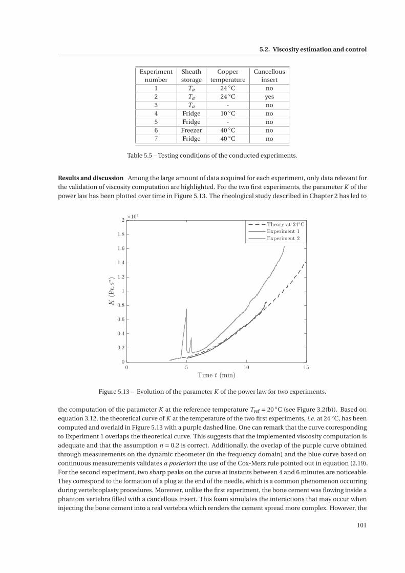
5.2. Viscosity estimation and control
Experiment Sheath Copper Cancellousnumber storage temperature insert
1 Ta 24 ◦C no2 Ta 24 ◦C yes3 Ta - no4 Fridge 10 ◦C no5 Fridge - no6 Freezer 40 ◦C no7 Fridge 40 ◦C no
Table 5.5 – Testing conditions of the conducted experiments.
Results and discussion Among the large amount of data acquired for each experiment, only data relevant for
the validation of viscosity computation are highlighted. For the two first experiments, the parameter K of the
power law has been plotted over time in Figure 5.13. The rheological study described in Chapter 2 has led to
0 5 10 15
Time t (min)
0
0.2
0.4
0.6
0.8
1
1.2
1.4
1.6
1.8
2
K(Pa.sn)
×104
Theory at 24◦C
Experiment 1
Experiment 2
Figure 5.13 – Evolution of the parameter K of the power law for two experiments.
the computation of the parameter K at the reference temperature Tref = 20 ◦C (see Figure 3.2(b)). Based on
equation 3.12, the theoretical curve of K at the temperature of the two first experiments, i.e. at 24 ◦C, has been
computed and overlaid in Figure 5.13 with a purple dashed line. One can remark that the curve corresponding
to Experiment 1 overlaps the theoretical curve. This suggests that the implemented viscosity computation is
adequate and that the assumption n = 0.2 is correct. Additionally, the overlap of the purple curve obtained
through measurements on the dynamic rheometer (in the frequency domain) and the blue curve based on
continuous measurements validates a posteriori the use of the Cox-Merz rule pointed out in equation (2.19).
For the second experiment, two sharp peaks on the curve at instants between 4 and 6 minutes are noticeable.
They correspond to the formation of a plug at the end of the needle, which is a common phenomenon occurring
during vertebroplasty procedures. Moreover, unlike the first experiment, the bone cement was flowing inside a
phantom vertebra filled with a cancellous insert. This foam simulates the interactions that may occur when
injecting the bone cement into a real vertebra which renders the cement spread more complex. However, the
101
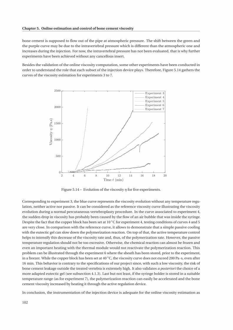
Chapter 5. Online estimation and control of bone cement viscosity
bone cement is supposed to flow out of the pipe at atmospheric pressure. The shift between the green and
the purple curve may be due to the intravertebral pressure which is different than the atmospheric one and
increases during the injection. For now, the intravertebral pressure has not been evaluated, that is why further
experiments have been achieved without any cancellous insert.
Besides the validation of the online viscosity computation, some other experiments have been conducted in
order to understand the role that each subset of the injection device plays. Therefore, Figure 5.14 gathers the
curves of the viscosity estimation for experiments 3 to 7.
2 4 6 8 10 12 14 16 18 20
Time t (min)
0
500
1000
1500
2000
2500
Viscosityη(Pa.s)
Experiment 3
Experiment 4
Experiment 5
Experiment 6
Experiment 7
Figure 5.14 – Evolution of the viscosity η for five experiments.
Corresponding to experiment 3, the blue curve represents the viscosity evolution without any temperature regu-
lation, neither active nor passive. It can be considered as the reference viscosity curve illustrating the viscosity
evolution during a normal percutaneous vertebroplasty procedure. In the curve associated to experiment 4,
the sudden drop in viscosity has probably been caused by the flow of an air bubble that was inside the syringe.
Despite the fact that the copper block has been set at 10 ◦C for experiment 4, testing conditions of curves 4 and 5
are very close. In comparison with the reference curve, it allows to demonstrate that a simple passive cooling
with the eutectic gel can slow down the polymerization reaction. On top of that, the active temperature control
helps to intensify this decrease of the viscosity rate and, thus, of the polymerization rate. However, the passive
temperature regulation should not be too excessive. Otherwise, the chemical reaction can almost be frozen and
even an important heating with the thermal module would not reactivate the polymerization reaction. This
problem can be illustrated through the experiment 6 where the sheath has been stored, prior to the experiment,
in a freezer. While the copper block has been set at 40 ◦C, the viscosity curve does not exceed 200 Pa·s, even after
16 min. This behavior is contrary to the specifications of our project since, with such a low viscosity, the risk of
bone cement leakage outside the treated vertebra is extremely high. It also validates a posteriori the choice of a
more adapted eutectic gel (see subsection 4.1.3). Last but not least, if the syringe holder is stored in a suitable
temperature range (as for experiment 7), the polymerization reaction can easily be accelerated and the bone
cement viscosity increased by heating it through the active regulation device.
In conclusion, the instrumentation of the injection device is adequate for the online viscosity estimation as
102
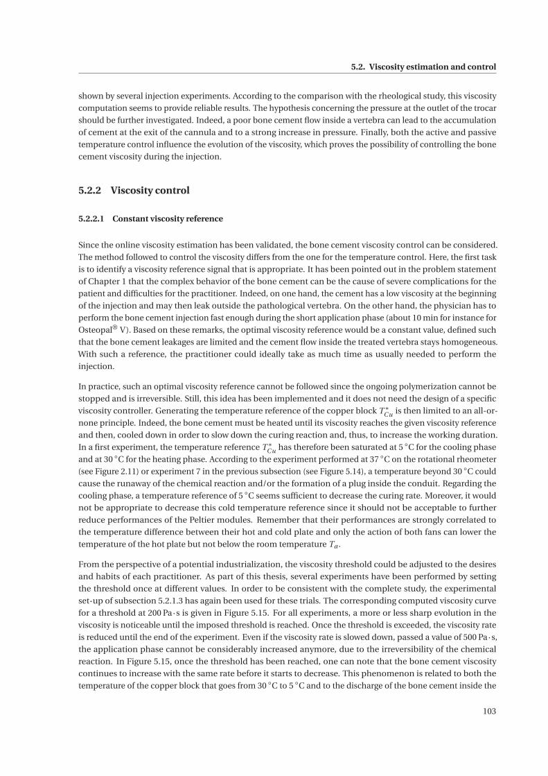
5.2. Viscosity estimation and control
shown by several injection experiments. According to the comparison with the rheological study, this viscosity
computation seems to provide reliable results. The hypothesis concerning the pressure at the outlet of the trocar
should be further investigated. Indeed, a poor bone cement flow inside a vertebra can lead to the accumulation
of cement at the exit of the cannula and to a strong increase in pressure. Finally, both the active and passive
temperature control influence the evolution of the viscosity, which proves the possibility of controlling the bone
cement viscosity during the injection.
5.2.2 Viscosity control
5.2.2.1 Constant viscosity reference
Since the online viscosity estimation has been validated, the bone cement viscosity control can be considered.
The method followed to control the viscosity differs from the one for the temperature control. Here, the first task
is to identify a viscosity reference signal that is appropriate. It has been pointed out in the problem statement
of Chapter 1 that the complex behavior of the bone cement can be the cause of severe complications for the
patient and difficulties for the practitioner. Indeed, on one hand, the cement has a low viscosity at the beginning
of the injection and may then leak outside the pathological vertebra. On the other hand, the physician has to
perform the bone cement injection fast enough during the short application phase (about 10 min for instance for
Osteopal® V). Based on these remarks, the optimal viscosity reference would be a constant value, defined such
that the bone cement leakages are limited and the cement flow inside the treated vertebra stays homogeneous.
With such a reference, the practitioner could ideally take as much time as usually needed to perform the
injection.
In practice, such an optimal viscosity reference cannot be followed since the ongoing polymerization cannot be
stopped and is irreversible. Still, this idea has been implemented and it does not need the design of a specific
viscosity controller. Generating the temperature reference of the copper block T ∗Cu is then limited to an all-or-
none principle. Indeed, the bone cement must be heated until its viscosity reaches the given viscosity reference
and then, cooled down in order to slow down the curing reaction and, thus, to increase the working duration.
In a first experiment, the temperature reference T ∗Cu has therefore been saturated at 5 ◦C for the cooling phase
and at 30 ◦C for the heating phase. According to the experiment performed at 37 ◦C on the rotational rheometer
(see Figure 2.11) or experiment 7 in the previous subsection (see Figure 5.14), a temperature beyond 30 ◦C could
cause the runaway of the chemical reaction and/or the formation of a plug inside the conduit. Regarding the
cooling phase, a temperature reference of 5 ◦C seems sufficient to decrease the curing rate. Moreover, it would
not be appropriate to decrease this cold temperature reference since it should not be acceptable to further
reduce performances of the Peltier modules. Remember that their performances are strongly correlated to
the temperature difference between their hot and cold plate and only the action of both fans can lower the
temperature of the hot plate but not below the room temperature Ta .
From the perspective of a potential industrialization, the viscosity threshold could be adjusted to the desires
and habits of each practitioner. As part of this thesis, several experiments have been performed by setting
the threshold once at different values. In order to be consistent with the complete study, the experimental
set-up of subsection 5.2.1.3 has again been used for these trials. The corresponding computed viscosity curve
for a threshold at 200 Pa·s is given in Figure 5.15. For all experiments, a more or less sharp evolution in the
viscosity is noticeable until the imposed threshold is reached. Once the threshold is exceeded, the viscosity rate
is reduced until the end of the experiment. Even if the viscosity rate is slowed down, passed a value of 500 Pa·s,
the application phase cannot be considerably increased anymore, due to the irreversibility of the chemical
reaction. In Figure 5.15, once the threshold has been reached, one can note that the bone cement viscosity
continues to increase with the same rate before it starts to decrease. This phenomenon is related to both the
temperature of the copper block that goes from 30 ◦C to 5 ◦C and to the discharge of the bone cement inside the
103
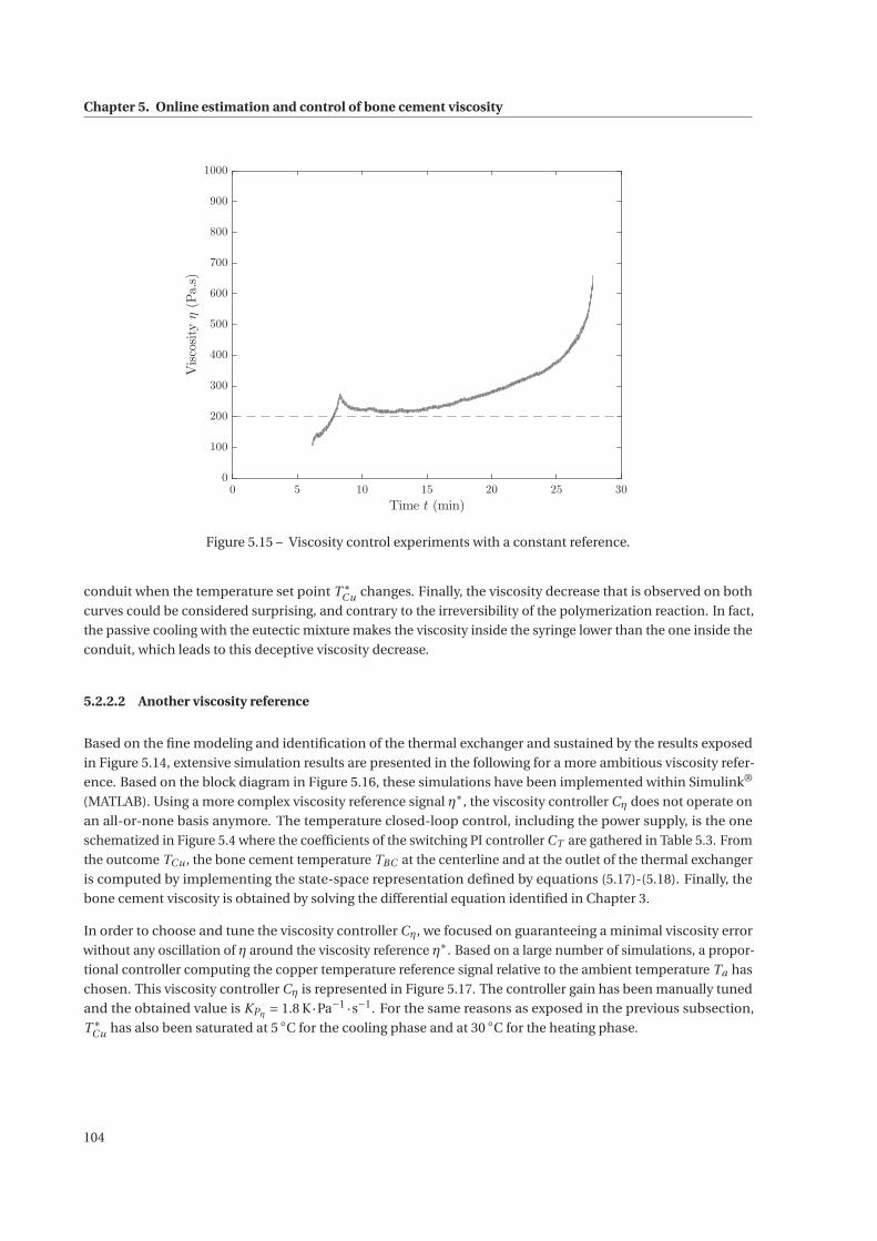
Chapter 5. Online estimation and control of bone cement viscosity
0 5 10 15 20 25 30
Time t (min)
0
100
200
300
400
500
600
700
800
900
1000
Viscosityη(Pa.s)
Figure 5.15 – Viscosity control experiments with a constant reference.
conduit when the temperature set point T ∗Cu changes. Finally, the viscosity decrease that is observed on both
curves could be considered surprising, and contrary to the irreversibility of the polymerization reaction. In fact,
the passive cooling with the eutectic mixture makes the viscosity inside the syringe lower than the one inside the
conduit, which leads to this deceptive viscosity decrease.
5.2.2.2 Another viscosity reference
Based on the fine modeling and identification of the thermal exchanger and sustained by the results exposed
in Figure 5.14, extensive simulation results are presented in the following for a more ambitious viscosity refer-
ence. Based on the block diagram in Figure 5.16, these simulations have been implemented within Simulink®
(MATLAB). Using a more complex viscosity reference signal η∗, the viscosity controller Cη does not operate on
an all-or-none basis anymore. The temperature closed-loop control, including the power supply, is the one
schematized in Figure 5.4 where the coefficients of the switching PI controller CT are gathered in Table 5.3. From
the outcome TCu , the bone cement temperature TBC at the centerline and at the outlet of the thermal exchanger
is computed by implementing the state-space representation defined by equations (5.17)-(5.18). Finally, the
bone cement viscosity is obtained by solving the differential equation identified in Chapter 3.
In order to choose and tune the viscosity controller Cη, we focused on guaranteeing a minimal viscosity error
without any oscillation of η around the viscosity reference η∗. Based on a large number of simulations, a propor-
tional controller computing the copper temperature reference signal relative to the ambient temperature Ta has
chosen. This viscosity controller Cη is represented in Figure 5.17. The controller gain has been manually tuned
and the obtained value is KPη = 1.8 K·Pa−1 ·s−1. For the same reasons as exposed in the previous subsection,
T ∗Cu has also been saturated at 5 ◦C for the cooling phase and at 30 ◦C for the heating phase.
104
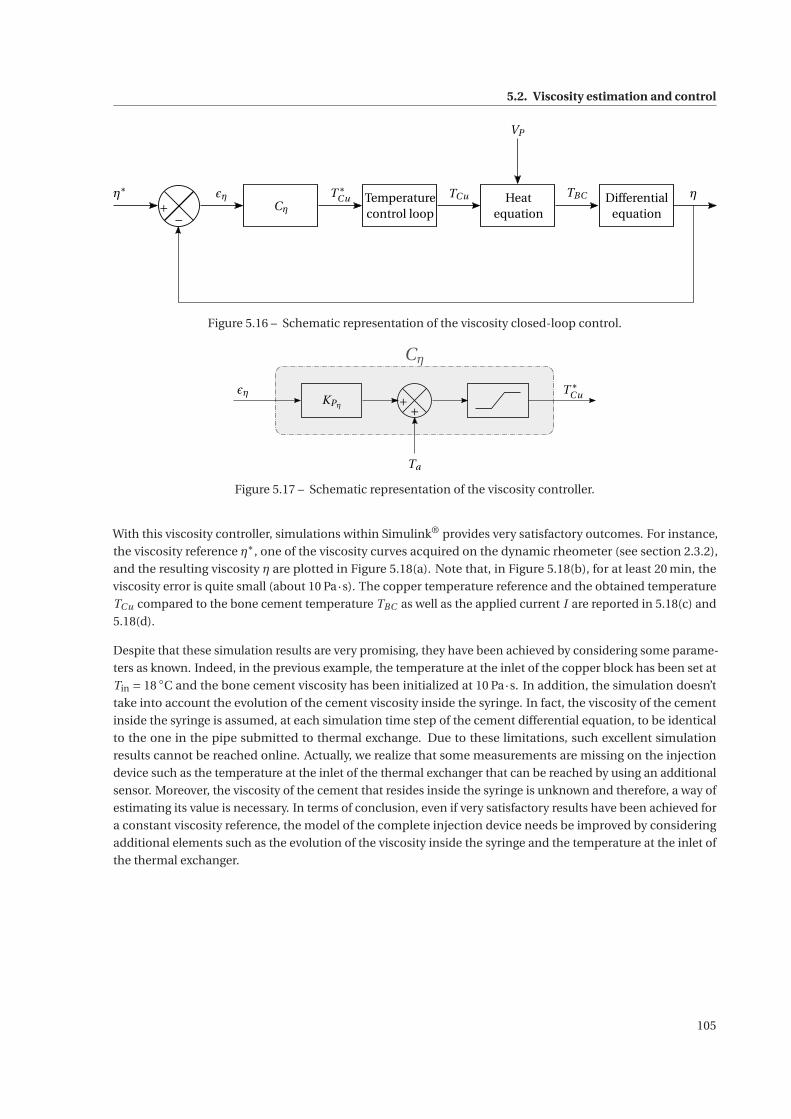
5.2. Viscosity estimation and control
η∗
+−
εηCη
T ∗Cu Temperature
control loop
TCu Heatequation
TBC ηDifferentialequation
VP
Figure 5.16 – Schematic representation of the viscosity closed-loop control.
εηKPη
T ∗Cu
Cη
+ +
Ta
Figure 5.17 – Schematic representation of the viscosity controller.
With this viscosity controller, simulations within Simulink® provides very satisfactory outcomes. For instance,
the viscosity reference η∗, one of the viscosity curves acquired on the dynamic rheometer (see section 2.3.2),
and the resulting viscosity η are plotted in Figure 5.18(a). Note that, in Figure 5.18(b), for at least 20 min, the
viscosity error is quite small (about 10 Pa·s). The copper temperature reference and the obtained temperature
TCu compared to the bone cement temperature TBC as well as the applied current I are reported in 5.18(c) and
5.18(d).
Despite that these simulation results are very promising, they have been achieved by considering some parame-
ters as known. Indeed, in the previous example, the temperature at the inlet of the copper block has been set at
Tin = 18 ◦C and the bone cement viscosity has been initialized at 10 Pa·s. In addition, the simulation doesn’t
take into account the evolution of the cement viscosity inside the syringe. In fact, the viscosity of the cement
inside the syringe is assumed, at each simulation time step of the cement differential equation, to be identical
to the one in the pipe submitted to thermal exchange. Due to these limitations, such excellent simulation
results cannot be reached online. Actually, we realize that some measurements are missing on the injection
device such as the temperature at the inlet of the thermal exchanger that can be reached by using an additional
sensor. Moreover, the viscosity of the cement that resides inside the syringe is unknown and therefore, a way of
estimating its value is necessary. In terms of conclusion, even if very satisfactory results have been achieved for
a constant viscosity reference, the model of the complete injection device needs be improved by considering
additional elements such as the evolution of the viscosity inside the syringe and the temperature at the inlet of
the thermal exchanger.
105
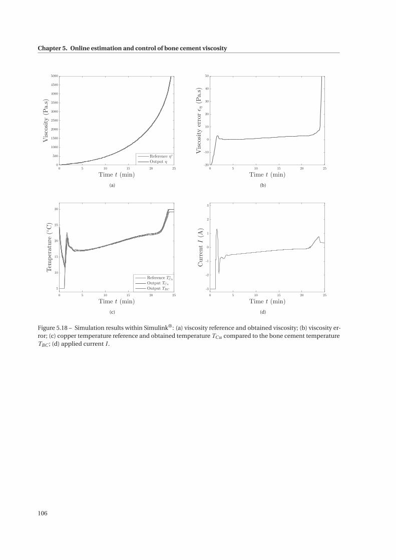
Chapter 5. Online estimation and control of bone cement viscosity
0 5 10 15 20 25
Time t (min)
0
500
1000
1500
2000
2500
3000
3500
4000
4500
5000
Viscosity(Pa.s)
Reference η∗
Output η
(a)
0 5 10 15 20 25
Time t (min)
-20
-10
0
10
20
30
40
50
Viscosityerrorεη(Pa.s)
(b)
0 5 10 15 20 25
Time t (min)
5
10
15
20
25
30
Temperature(◦C)
Reference T∗
Cu
Output TCu
Output TBC
(c)
0 5 10 15 20 25
Time t (min)
-3
-2
-1
0
1
2
3
CurrentI(A)
(d)
Figure 5.18 – Simulation results within Simulink®: (a) viscosity reference and obtained viscosity; (b) viscosity er-ror; (c) copper temperature reference and obtained temperature TCu compared to the bone cement temperatureTBC ; (d) applied current I .
106
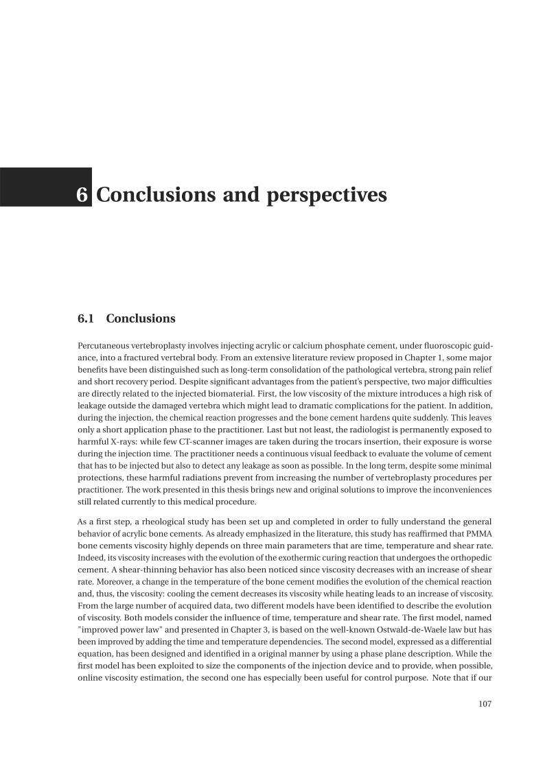
6 Conclusions and perspectives
6.1 Conclusions
Percutaneous vertebroplasty involves injecting acrylic or calcium phosphate cement, under fluoroscopic guid-
ance, into a fractured vertebral body. From an extensive literature review proposed in Chapter 1, some major
benefits have been distinguished such as long-term consolidation of the pathological vertebra, strong pain relief
and short recovery period. Despite significant advantages from the patient’s perspective, two major difficulties
are directly related to the injected biomaterial. First, the low viscosity of the mixture introduces a high risk of
leakage outside the damaged vertebra which might lead to dramatic complications for the patient. In addition,
during the injection, the chemical reaction progresses and the bone cement hardens quite suddenly. This leaves
only a short application phase to the practitioner. Last but not least, the radiologist is permanently exposed to
harmful X-rays: while few CT-scanner images are taken during the trocars insertion, their exposure is worse
during the injection time. The practitioner needs a continuous visual feedback to evaluate the volume of cement
that has to be injected but also to detect any leakage as soon as possible. In the long term, despite some minimal
protections, these harmful radiations prevent from increasing the number of vertebroplasty procedures per
practitioner. The work presented in this thesis brings new and original solutions to improve the inconveniences
still related currently to this medical procedure.
As a first step, a rheological study has been set up and completed in order to fully understand the general
behavior of acrylic bone cements. As already emphasized in the literature, this study has reaffirmed that PMMA
bone cements viscosity highly depends on three main parameters that are time, temperature and shear rate.
Indeed, its viscosity increases with the evolution of the exothermic curing reaction that undergoes the orthopedic
cement. A shear-thinning behavior has also been noticed since viscosity decreases with an increase of shear
rate. Moreover, a change in the temperature of the bone cement modifies the evolution of the chemical reaction
and, thus, the viscosity: cooling the cement decreases its viscosity while heating leads to an increase of viscosity.
From the large number of acquired data, two different models have been identified to describe the evolution
of viscosity. Both models consider the influence of time, temperature and shear rate. The first model, named
"improved power law" and presented in Chapter 3, is based on the well-known Ostwald-de-Waele law but has
been improved by adding the time and temperature dependencies. The second model, expressed as a differential
equation, has been designed and identified in a original manner by using a phase plane description. While the
first model has been exploited to size the components of the injection device and to provide, when possible,
online viscosity estimation, the second one has especially been useful for control purpose. Note that if our
107
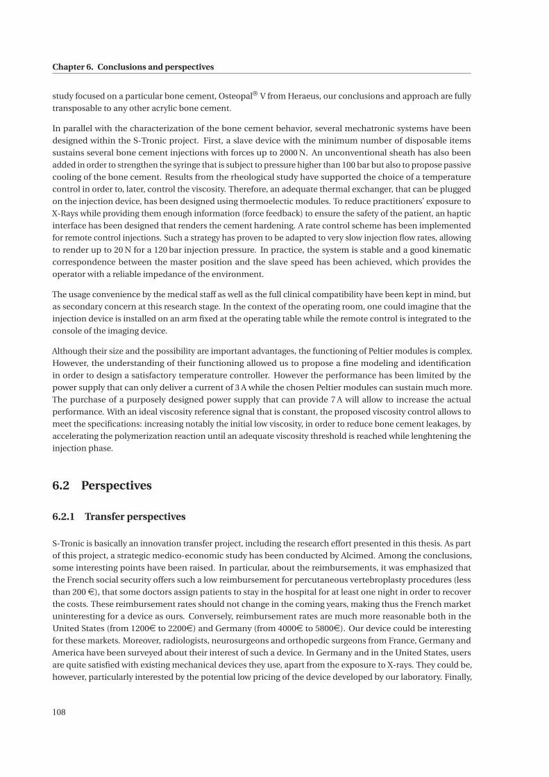
Chapter 6. Conclusions and perspectives
study focused on a particular bone cement, Osteopal® V from Heraeus, our conclusions and approach are fully
transposable to any other acrylic bone cement.
In parallel with the characterization of the bone cement behavior, several mechatronic systems have been
designed within the S-Tronic project. First, a slave device with the minimum number of disposable items
sustains several bone cement injections with forces up to 2000 N. An unconventional sheath has also been
added in order to strengthen the syringe that is subject to pressure higher than 100 bar but also to propose passive
cooling of the bone cement. Results from the rheological study have supported the choice of a temperature
control in order to, later, control the viscosity. Therefore, an adequate thermal exchanger, that can be plugged
on the injection device, has been designed using thermoelectic modules. To reduce practitioners’ exposure to
X-Rays while providing them enough information (force feedback) to ensure the safety of the patient, an haptic
interface has been designed that renders the cement hardening. A rate control scheme has been implemented
for remote control injections. Such a strategy has proven to be adapted to very slow injection flow rates, allowing
to render up to 20 N for a 120 bar injection pressure. In practice, the system is stable and a good kinematic
correspondence between the master position and the slave speed has been achieved, which provides the
operator with a reliable impedance of the environment.
The usage convenience by the medical staff as well as the full clinical compatibility have been kept in mind, but
as secondary concern at this research stage. In the context of the operating room, one could imagine that the
injection device is installed on an arm fixed at the operating table while the remote control is integrated to the
console of the imaging device.
Although their size and the possibility are important advantages, the functioning of Peltier modules is complex.
However, the understanding of their functioning allowed us to propose a fine modeling and identification
in order to design a satisfactory temperature controller. However the performance has been limited by the
power supply that can only deliver a current of 3 A while the chosen Peltier modules can sustain much more.
The purchase of a purposely designed power supply that can provide 7 A will allow to increase the actual
performance. With an ideal viscosity reference signal that is constant, the proposed viscosity control allows to
meet the specifications: increasing notably the initial low viscosity, in order to reduce bone cement leakages, by
accelerating the polymerization reaction until an adequate viscosity threshold is reached while lenghtening the
injection phase.
6.2 Perspectives
6.2.1 Transfer perspectives
S-Tronic is basically an innovation transfer project, including the research effort presented in this thesis. As part
of this project, a strategic medico-economic study has been conducted by Alcimed. Among the conclusions,
some interesting points have been raised. In particular, about the reimbursements, it was emphasized that
the French social security offers such a low reimbursement for percutaneous vertebroplasty procedures (less
than 200e), that some doctors assign patients to stay in the hospital for at least one night in order to recover
the costs. These reimbursement rates should not change in the coming years, making thus the French market
uninteresting for a device as ours. Conversely, reimbursement rates are much more reasonable both in the
United States (from 1200e to 2200e) and Germany (from 4000e to 5800e). Our device could be interesting
for these markets. Moreover, radiologists, neurosurgeons and orthopedic surgeons from France, Germany and
America have been surveyed about their interest of such a device. In Germany and in the United States, users
are quite satisfied with existing mechanical devices they use, apart from the exposure to X-rays. They could be,
however, particularly interested by the potential low pricing of the device developed by our laboratory. Finally,
108
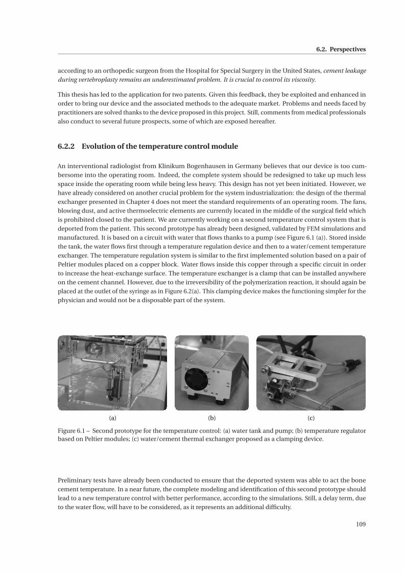
6.2. Perspectives
according to an orthopedic surgeon from the Hospital for Special Surgery in the United States, cement leakage
during vertebroplasty remains an underestimated problem. It is crucial to control its viscosity.
This thesis has led to the application for two patents. Given this feedback, they be exploited and enhanced in
order to bring our device and the associated methods to the adequate market. Problems and needs faced by
practitioners are solved thanks to the device proposed in this project. Still, comments from medical professionals
also conduct to several future prospects, some of which are exposed hereafter.
6.2.2 Evolution of the temperature control module
An interventional radiologist from Klinikum Bogenhausen in Germany believes that our device is too cum-
bersome into the operating room. Indeed, the complete system should be redesigned to take up much less
space inside the operating room while being less heavy. This design has not yet been initiated. However, we
have already considered on another crucial problem for the system industrialization: the design of the thermal
exchanger presented in Chapter 4 does not meet the standard requirements of an operating room. The fans,
blowing dust, and active thermoelectric elements are currently located in the middle of the surgical field which
is prohibited closed to the patient. We are currently working on a second temperature control system that is
deported from the patient. This second prototype has already been designed, validated by FEM simulations and
manufactured. It is based on a circuit with water that flows thanks to a pump (see Figure 6.1 (a)). Stored inside
the tank, the water flows first through a temperature regulation device and then to a water/cement temperature
exchanger. The temperature regulation system is similar to the first implemented solution based on a pair of
Peltier modules placed on a copper block. Water flows inside this copper through a specific circuit in order
to increase the heat-exchange surface. The temperature exchanger is a clamp that can be installed anywhere
on the cement channel. However, due to the irreversibility of the polymerization reaction, it should again be
placed at the outlet of the syringe as in Figure 6.2(a). This clamping device makes the functioning simpler for the
physician and would not be a disposable part of the system.
(a) (c)(b)
Figure 6.1 – Second prototype for the temperature control: (a) water tank and pump; (b) temperature regulatorbased on Peltier modules; (c) water/cement thermal exchanger proposed as a clamping device.
Preliminary tests have already been conducted to ensure that the deported system was able to act the bone
cement temperature. In a near future, the complete modeling and identification of this second prototype should
lead to a new temperature control with better performance, according to the simulations. Still, a delay term, due
to the water flow, will have to be considered, as it represents an additional difficulty.
109
Chapter 6. Conclusions and perspectives
(a) (b)
Figure 6.2 – CAD views: (a) clamp used as a water/cement thermal exchanger; (b) experimental scenario withthe second prototype.
6.2.3 Intravertebral pressure
In Chapter 5, the assumption that bone cement flows out of the conduit at atmospheric pressure has been
challenged, especially when the cement has been injected into a phantom vertebra including a cancellous insert.
In the literature, some studies on cadavers have been carried out in order to picture the intravertebral pressure
during a cement injection. Here, thanks to our device and methods, a perspective would be to compute online
this intravertebral pressure. On the clamp of the future prototype, a pressure sensor has been installed. The
previous online approach to compute viscosity can also lead to the intravertebral pressure Pvertebra for a distance
Lvertebra to the vertebra. This sensor is positioned at a known length Lsensor from the outlet of the syringe and on
the pipe in which flows the bone cement while bearing Lsensor >> R as illustrated in figure 6.3.
Pressure sensor Vertebra
Syringe
Lsensor
Lvertebra
Figure 6.3 – Geometry of the pipe coming out of the syringe and going inside the vertebra.
On both the section of length Lsensor and Lvertebra, equation 5.30 could be applied. Assuming that the flow rate is
high enough, the cement viscosity at the sensor should be substantially equal to the one at the outlet. Then,
knowing that the flow rate is constant in the pipe, the following equality holds:
ΔPsensor
Lsensor= ΔPvertebra
Lvertebra(6.1)
where ΔPsensor (respectively ΔPvertebra) represents the pressure drop over Lsensor (respectively Lvertebra). Finally,
the intravertebral pressure could be accessed as:
Pvertebra =F
πR2s
(1− Lvertebra
Lsensor
)+ Lvertebra
LsensorPsensor. (6.2)
where F is the force applied to the piston and Rs the radius of the syringe.
110
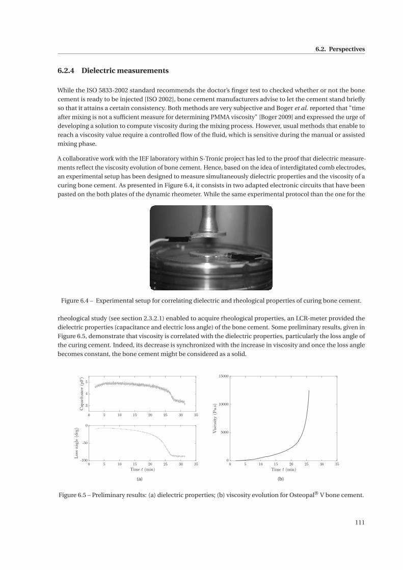
6.2. Perspectives
6.2.4 Dielectric measurements
While the ISO 5833-2002 standard recommends the doctor’s finger test to checked whether or not the bone
cement is ready to be injected [ISO 2002], bone cement manufacturers advise to let the cement stand briefly
so that it attains a certain consistency. Both methods are very subjective and Boger et al. reported that "time
after mixing is not a sufficient measure for determining PMMA viscosity" [Boger 2009] and expressed the urge of
developing a solution to compute viscosity during the mixing process. However, usual methods that enable to
reach a viscosity value require a controlled flow of the fluid, which is sensitive during the manual or assisted
mixing phase.
A collaborative work with the IEF laboratory within S-Tronic project has led to the proof that dielectric measure-
ments reflect the viscosity evolution of bone cement. Hence, based on the idea of interdigitated comb electrodes,
an experimental setup has been designed to measure simultaneously dielectric properties and the viscosity of a
curing bone cement. As presented in Figure 6.4, it consists in two adapted electronic circuits that have been
pasted on the both plates of the dynamic rheometer. While the same experimental protocol than the one for the
Figure 6.4 – Experimental setup for correlating dielectric and rheological properties of curing bone cement.
rheological study (see section 2.3.2.1) enabled to acquire rheological properties, an LCR-meter provided the
dielectric properties (capacitance and electric loss angle) of the bone cement. Some preliminary results, given in
Figure 6.5, demonstrate that viscosity is correlated with the dielectric properties, particularly the loss angle of
the curing cement. Indeed, its decrease is synchronized with the increase in viscosity and once the loss angle
becomes constant, the bone cement might be considered as a solid.
0 5 10 15 20 25 30 35
3
4
5
Capacitance(pF)
0 5 10 15 20 25 30 35
Time t (min)
-100
-50
0
Lossangle
(deg)
(a)
0 5 10 15 20 25 30 35
Time t (min)
0
5000
10000
15000
Viscosity(Pa.s)
(b)
Figure 6.5 – Preliminary results: (a) dielectric properties; (b) viscosity evolution for Osteopal® V bone cement.
111
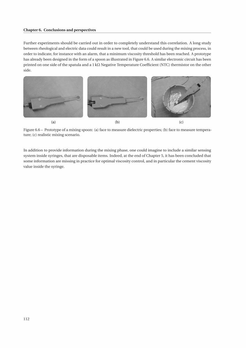
Chapter 6. Conclusions and perspectives
Further experiments should be carried out in order to completely understand this correlation. A long study
between rheological and electric data could result in a new tool, that could be used during the mixing process, in
order to indicate, for instance with an alarm, that a minimum viscosity threshold has been reached. A prototype
has already been designed in the form of a spoon as illustrated in Figure 6.6. A similar electronic circuit has been
printed on one side of the spatula and a 1 kΩ Negative Temperature Coefficient (NTC) thermistor on the other
side.
(a) (c)(b)
Figure 6.6 – Prototype of a mixing spoon: (a) face to measure dielectric properties; (b) face to measure tempera-ture; (c) realistic mixing scenario.
In addition to provide information during the mixing phase, one could imagine to include a similar sensing
system inside syringes, that are disposable items. Indeed, at the end of Chapter 5, it has been concluded that
some information are missing in practice for optimal viscosity control, and in particular the cement viscosity
value inside the syringe.
112
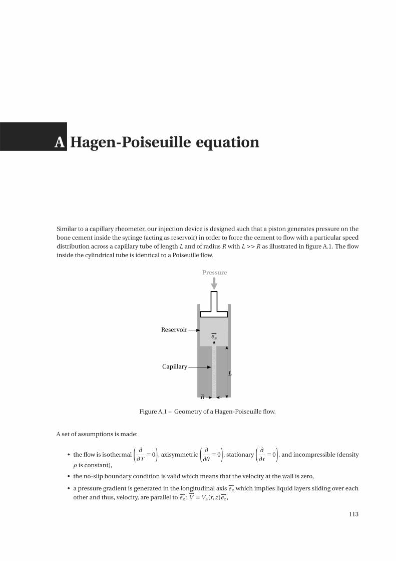
A Hagen-Poiseuille equation
Similar to a capillary rheometer, our injection device is designed such that a piston generates pressure on the
bone cement inside the syringe (acting as reservoir) in order to force the cement to flow with a particular speed
distribution across a capillary tube of length L and of radius R with L >> R as illustrated in figure A.1. The flow
inside the cylindrical tube is identical to a Poiseuille flow.
R
L
−→ez
Pressure
Reservoir
Capillary
Figure A.1 – Geometry of a Hagen-Poiseuille flow.
A set of assumptions is made:
• the flow is isothermal
(∂
∂T≡ 0
), axisymmetric
(∂
∂θ≡ 0
), stationary
(∂
∂t≡ 0
), and incompressible (density
ρ is constant),
• the no-slip boundary condition is valid which means that the velocity at the wall is zero,
• a pressure gradient is generated in the longitudinal axis −→ez which implies liquid layers sliding over each
other and thus, velocity, are parallel to −→ez :−→V =Vz (r, z)−→ez ,
113
Appendix A. Hagen-Poiseuille equation
• the pressure gradient is assumed to be negative when the flow is in the direction of positive z.
The symmetric strain rate tensor, defined as D = 1
2
(∇V + (∇V )T
), is written in our specific context as follows:
[D]=
⎛⎜⎜⎝
0 0 12∂Vz∂r
0 0 012∂Vz∂r 0 ∂Vz
∂z
⎞⎟⎟⎠
(−→e r ,−→e θ ,−→e z )
. (A.1)
For a generalized Newtonian flow, the relation between the strain rate tensor and the Cauchy stress tensor is
expressed as:
σ=−pI+2ηD+(κ− 2
3η
)−→∇ .−→V I (A.2)
where:
• p is the applied pressure,
• I represents the third-order identity tensor,
• η denotes the dynamic viscosity of the fluid,
• κ is the bulk viscosity,
• γ=2IID is the magnitude of the strain rate tensor. In the frame of some simple geometries of the flow, γ
designates the shear rate,
• IID, second invariant of D.
In fluid dynamics, the principle of mass conservation states:
∂ρ
∂t+ρ
−→∇ ·−→V = 0 (A.3)
Since the assumption is made that the fluid is incompressible, equation (A.3) leads to−→∇ ·
−→V = 0 which simplifies
• equation (A.2) as:
σ=−pI+2η(γ)D , (A.4)
• the last component of−→V as:
Vz ≡Vz (r ). (A.5)
Considering equation (A.4) and the simplification (A.5), the stress tensor is expressed in the coordinate reference
(−→er ,−→eθ,−→ez ) as:
[σ
]=
⎛⎜⎜⎝−p 0 η∂Vz
∂r
0 −p 0
η∂Vz∂r 0 −p
⎞⎟⎟⎠
(−→er ,−→eθ ,−→ez )
. (A.6)
114
Governing the motion of fluids, the general Navier-Stokes equation yields:
ρD−→V
Dt=−→∇ ·σ+ρ
−→g (A.7)
with:
• D−→V
Dt = ∂−→V∂t + (
−→V ·∇)
−→V , the material derivative of the velocity vector field,
• −→g , the gravitational field.
Given the stationary assumption, we can assess:
∂−→V
∂t=−→
0 (A.8)
Moreover,
(−→V ·∇)
−→V =Vz
∂Vz
∂z−→ez =−→
0 (A.9)
Thus, while neglecting gravity, Navier-Stokes equation (equation (A.7)) can be projected in the cylindrical
coordinate system and provides:
−∂p
∂r= 0 (A.10)
−1
r
∂p
∂θ= 0 (A.11)
−∂p
∂z+ 1
r
∂rσ′r z
∂r= 0 (A.12)
where σ′ = 2η(γ)D.
From equation (A.12), using the separation of variables, we obtain:
∂p
∂z=−ΔP
L(A.13)
with ΔP = Pinlet −Poutlet > 0, the pressure drop along the capillary of length L.
Then, the integration of equation (A.12) gives:
σ′r z (r ) =−ΔP
L
r
2+ constant
r(A.14)
On the symmetry axis, the boundary condition is∂Vz (r )
∂r
∣∣∣∣r=0
= 0, the following relation is achieved:
σ′r z (r ) =−ΔP
L
r
2. (A.15)
This relation is valid no matter the behavior law of the dynamic viscosity of the fluid. From here on, the behavior
law has to be defined. For bone cement, we can assess that it follows the Ostwald-de Waele law [Ostwald 1925],
commonly called Power-law, which is given by :
η(γ) = K γn−1 (A.16)
115
Appendix A. Hagen-Poiseuille equation
where K represents the consistency in Pa.sn and n the power law index.
According to equation (A.6), it can be written:
σ′r z = η(γ)
∂Vz (r )
∂rwith γ=−∂Vz (r )
∂r. (A.17)
From equations (A.16) and (A.17), σ′r z is equivalent to:
σ′r z =−K
(−∂Vz (r )
∂r
)n
. (A.18)
By substituting σ′r z with its expression (A.15) and by integrating this last equation, Vz (r ) can be computed as:
Vz (r ) =− n
n +1
(ΔP
2K L
) 1n
rn+1
n +constant. (A.19)
Taking into account the no-slip boundary condition, we obtain:
Vz (r ) = n
n +1
(ΔP
2K L
) 1n (
Rn+1
n − rn+1
n
). (A.20)
Finally, we can compute flow rate Q and shear rate at the wall γp :
Q =∫R
0Vz (r )2πr dr =
(ΔP
L
) 1n(
R
2K
) 1n(πnR3
3n +1
)(A.21)
γp = −∂Vz (r )
∂r
∣∣∣∣r=R
= Q
πR3
3n +1
n. (A.22)
For comparison, for a Newtonian-fluid (i.e. η= η0), Vz , Q and γp are expressed as follows:
Vz (r ) = ΔP
4η0L
(R2 − r 2) (A.23)
Q = ΔPπR4
8η0L(A.24)
γp = 4Q
πR3 . (A.25)
The relationship between flow rate Q and pressure drop ΔP in (A.21) is called Hagen-Poiseuille equation.
116
B Transient convective heat transfer
This appendix aims to present the analytic solution of the transient heat conduction of an infinite cylinder of
radius R. This problem is axisymmetric and T (r, t ) represents the temperature at time t and at a radius r from
the centerline. The heat equation yields:
ρc∂T
∂t=λ
−→∇ ·(−→∇T
)(B.1)
where ρ, c and λ are the density, the specific heat capacity and the thermal conductivity, respectively. The
considered material is not flowing and no terms of heat creation have been added. The initial temperature is
such that:
T (r,0) = Tinit (B.2)
At time t > 0, the sample is subjected to free convection, with a heat transfer coefficient h, with the surrounding
environment at T∞, which writes:
−λ∂T
∂r|r=Rc = h (T −T∞) (B.3)
Using advanced mathematical methods, the general solution of the transient homogeneous heat conduction
can be written in the form of an infinite series as:
T (r, t )−T∞Tinit −T∞
=∞∑
j=1B j exp
(−ω2
j F0
)J0
(ω j
r
Rc
)(B.4)
where:
• B j =2
ω j.
J1(ω j
)J 2
0
(ω j
)+ J 2
1
(ω j
)• J0 and J1 are the Bessel functions of the first kind, defined as:
Ji (x) =∞∑
p=0
(−1)p
p !(n +p)!
(x
2
)2p +n , (B.5)
117
Appendix B. Transient convective heat transfer
• F0 is the Fourier number with F0 =αt
R2c= λt
ρcR2c
,
• ω j are the eigen values of ω j J1(ω j ) = Bi J0(ω j ),
• Bi is the Biot number such that Bi = hRc
2λ,
Hence, since J0(0) = 1 at the centerline, i.e. for r = 0, equation (B.4) becomes:
T (0, t )−T∞Tinit −T∞
=∞∑
j=1B j exp
(−ω2
j F0
)(B.6)
118
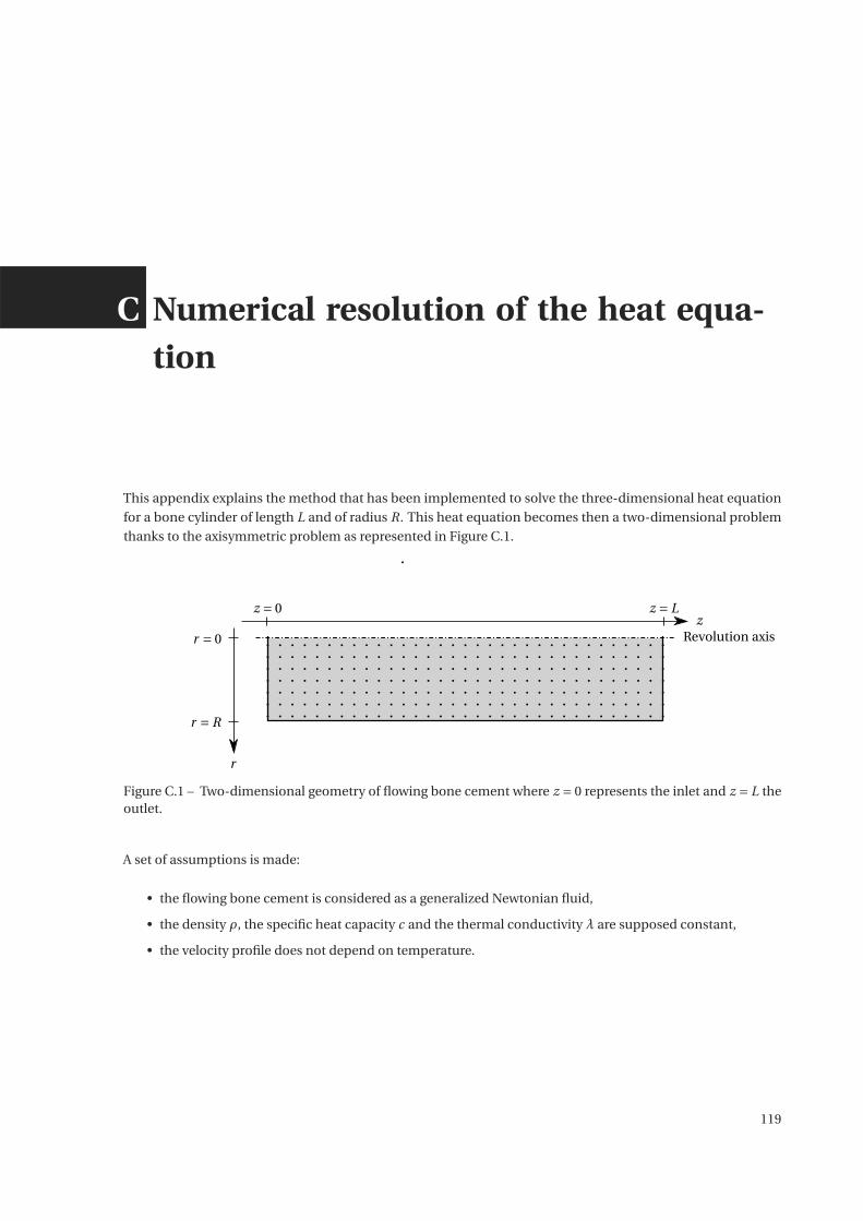
C Numerical resolution of the heat equa-tion
This appendix explains the method that has been implemented to solve the three-dimensional heat equation
for a bone cylinder of length L and of radius R. This heat equation becomes then a two-dimensional problem
thanks to the axisymmetric problem as represented in Figure C.1.
zz = 0 z = L
r = 0
r = R
Revolution axis
r
Figure C.1 – Two-dimensional geometry of flowing bone cement where z = 0 represents the inlet and z = L theoutlet.
A set of assumptions is made:
• the flowing bone cement is considered as a generalized Newtonian fluid,
• the density ρ, the specific heat capacity c and the thermal conductivity λ are supposed constant,
• the velocity profile does not depend on temperature.
119
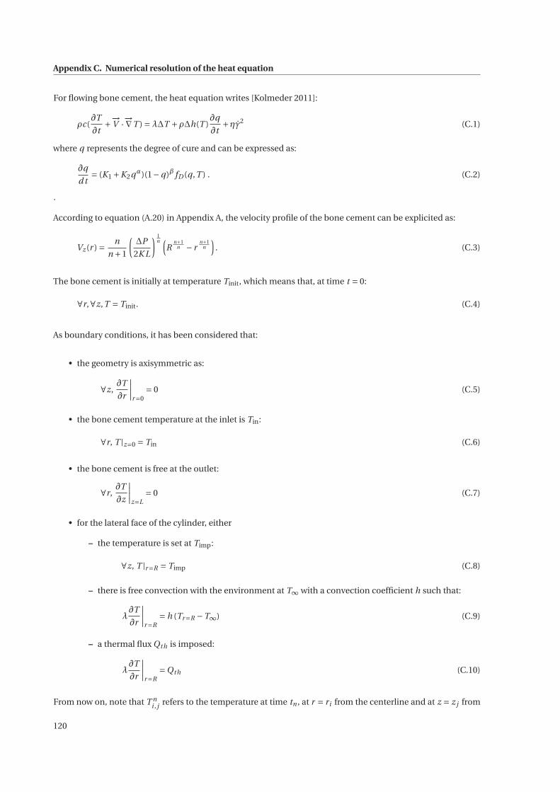
Appendix C. Numerical resolution of the heat equation
For flowing bone cement, the heat equation writes [Kolmeder 2011]:
ρc(∂T
∂t+−→
V ·−→∇T ) =λΔT +ρΔh(T )
∂q
∂t+ηγ2 (C.1)
where q represents the degree of cure and can be expressed as:
∂q
d t= (K1 +K2qα)(1−q)β fD (q,T ) . (C.2)
.
According to equation (A.20) in Appendix A, the velocity profile of the bone cement can be explicited as:
Vz (r ) = n
n +1
(ΔP
2K L
) 1n (
Rn+1
n − rn+1
n
). (C.3)
The bone cement is initially at temperature Tinit, which means that, at time t = 0:
∀r,∀z,T = Tinit. (C.4)
As boundary conditions, it has been considered that:
• the geometry is axisymmetric as:
∀z,∂T
∂r
∣∣∣∣r=0
= 0 (C.5)
• the bone cement temperature at the inlet is Tin:
∀r, T |z=0 = Tin (C.6)
• the bone cement is free at the outlet:
∀r,∂T
∂z
∣∣∣∣z=L
= 0 (C.7)
• for the lateral face of the cylinder, either
– the temperature is set at Timp:
∀z, T |r=R = Timp (C.8)
– there is free convection with the environment at T∞ with a convection coefficient h such that:
λ∂T
∂r
∣∣∣∣r=R
= h (Tr=R −T∞) (C.9)
– a thermal flux Qth is imposed:
λ∂T
∂r
∣∣∣∣r=R
=Qth (C.10)
From now on, note that T ni , j refers to the temperature at time tn , at r = ri from the centerline and at z = z j from
120
the inlet:
T ni , j = T
(ri , z j , tn
)(C.11)
Based on the finite-difference methods, a space discretization has been performed such that:
(∂T
∂r
)n
i , j�
T ni+1, j −T n
i−1, j
2Δr(C.12)
(∂2T
∂2r
)n
i , j�
T ni+1, j −2T n
i , j +T ni−1, j
Δr 2 (C.13)
(∂T
∂z
)n
i , j�
T ni , j+1 −T n
i , j−1
2Δz(C.14)
(∂2T
∂2z
)n
i , j�
T ni , j+1 −2T n
i , j +T ni , j−1
Δz2 (C.15)
After that this spatial finite difference discretization has been achieved, the discretized heat equation can be
written as a system of Ordinary Differential Equations (ODE) as:
M
[Tq
]= A
[Tq
]+B (C.16)
where M is a mass matrix and T is the vector that concatenates all temperatures Ti , j . A is a five-diagonal matrix.
Thanks to the function ode45 from MATLAB [MathWorks 2016], this system is numerically solved and the
evolution of each temperature Ti , j can be plotted.
121

D Résumé en français
D.1 Contexte médical
La vertébroplastie percutanée est une intervention non chirurgicale et peu invasive qui consiste à injecter, sous
contrôle radioscopique, un ciment orthopédique (PMMA) dans le corps vertébral. Cette technique permet
de stabiliser les vertèbres et de réduire les douleurs sévères chez les personnes souffrant principalement
d’ostéoporose, mais aussi de métastases ou de fractures traumatiques. Cette approche est particulièrement
efficace, puisqu’elle permet de stabiliser la vertèbre fracturée de manière durable. De plus, une amélioration
immédiate de la douleur chez les patients et leur lever précoce sont observés.
Malgré son efficacité, cette méthode présente quelques inconvénients non négligeables. Le premier tient au
ciment orthopédique, qui est injecté pendant sa phase de polymérisation. Tout d’abord, la faible viscosité du
ciment au début de l’injection augmente considérablement le risque de fuite en dehors de la vertèbre traitée,
ce qui provoque potentiellement des complications sévères. La prise rapide du ciment limite par ailleurs la
durée d’injection à huit à dix minutes maximum, selon le modèle de ciment. Le second inconvénient est lié au
contrôle par fluoroscopie à rayons X, qui expose le praticien de manière prolongée.
Pour pallier ces inconvénients, les enjeux de ce travail de thèse étaient :
• la caractérisation du comportement rhéologique du ciment,
• la maîtrise des paramètres influençant sa viscosité, et
• le développement d’un système robotisé télé-opéré avec un retour d’effort.
Actuellement, les systèmes d’injection manuels sont très nombreux sur le marché mais ne répondent aucune-
ment à la problématique de l’exposition des radiologues aux rayons X. Les systèmes télé-opérés sont quant à eux
très rares, et à notre connaissance, soit ils n’offrent pas de retour d’effort, soit ils n’éloignent pas le praticien
de la source des rayons X. Dans le travail présenté, le développement d’un système d’injection robotisée de
ciment orthopédique permet la radioprotection des praticiens, une réduction des risques de fuite et une durée
d’injection plus longue.
123
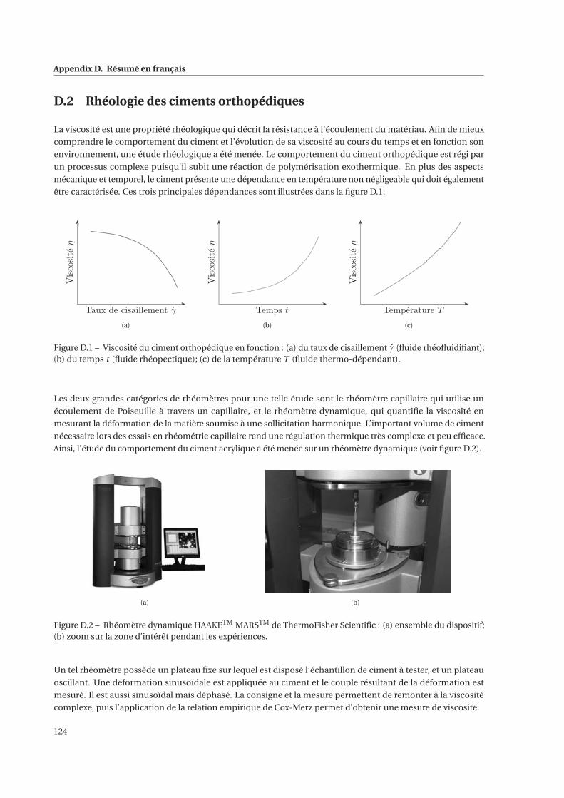
Appendix D. Résumé en français
D.2 Rhéologie des ciments orthopédiques
La viscosité est une propriété rhéologique qui décrit la résistance à l’écoulement du matériau. Afin de mieux
comprendre le comportement du ciment et l’évolution de sa viscosité au cours du temps et en fonction son
environnement, une étude rhéologique a été menée. Le comportement du ciment orthopédique est régi par
un processus complexe puisqu’il subit une réaction de polymérisation exothermique. En plus des aspects
mécanique et temporel, le ciment présente une dépendance en température non négligeable qui doit également
être caractérisée. Ces trois principales dépendances sont illustrées dans la figure D.1.
Taux de cisaillement γ
Viscositeη
(a)
Temps t
Viscositeη
(b)
Temperature T
Viscositeη
(c)
Figure D.1 – Viscosité du ciment orthopédique en fonction : (a) du taux de cisaillement γ (fluide rhéofluidifiant);(b) du temps t (fluide rhéopectique); (c) de la température T (fluide thermo-dépendant).
Les deux grandes catégories de rhéomètres pour une telle étude sont le rhéomètre capillaire qui utilise un
écoulement de Poiseuille à travers un capillaire, et le rhéomètre dynamique, qui quantifie la viscosité en
mesurant la déformation de la matière soumise à une sollicitation harmonique. L’important volume de ciment
nécessaire lors des essais en rhéométrie capillaire rend une régulation thermique très complexe et peu efficace.
Ainsi, l’étude du comportement du ciment acrylique a été menée sur un rhéomètre dynamique (voir figure D.2).
(a) (b)
Figure D.2 – Rhéomètre dynamique HAAKETM MARSTM de ThermoFisher Scientific : (a) ensemble du dispositif;(b) zoom sur la zone d’intérêt pendant les expériences.
Un tel rhéomètre possède un plateau fixe sur lequel est disposé l’échantillon de ciment à tester, et un plateau
oscillant. Une déformation sinusoïdale est appliquée au ciment et le couple résultant de la déformation est
mesuré. Il est aussi sinusoïdal mais déphasé. La consigne et la mesure permettent de remonter à la viscosité
complexe, puis l’application de la relation empirique de Cox-Merz permet d’obtenir une mesure de viscosité.
124
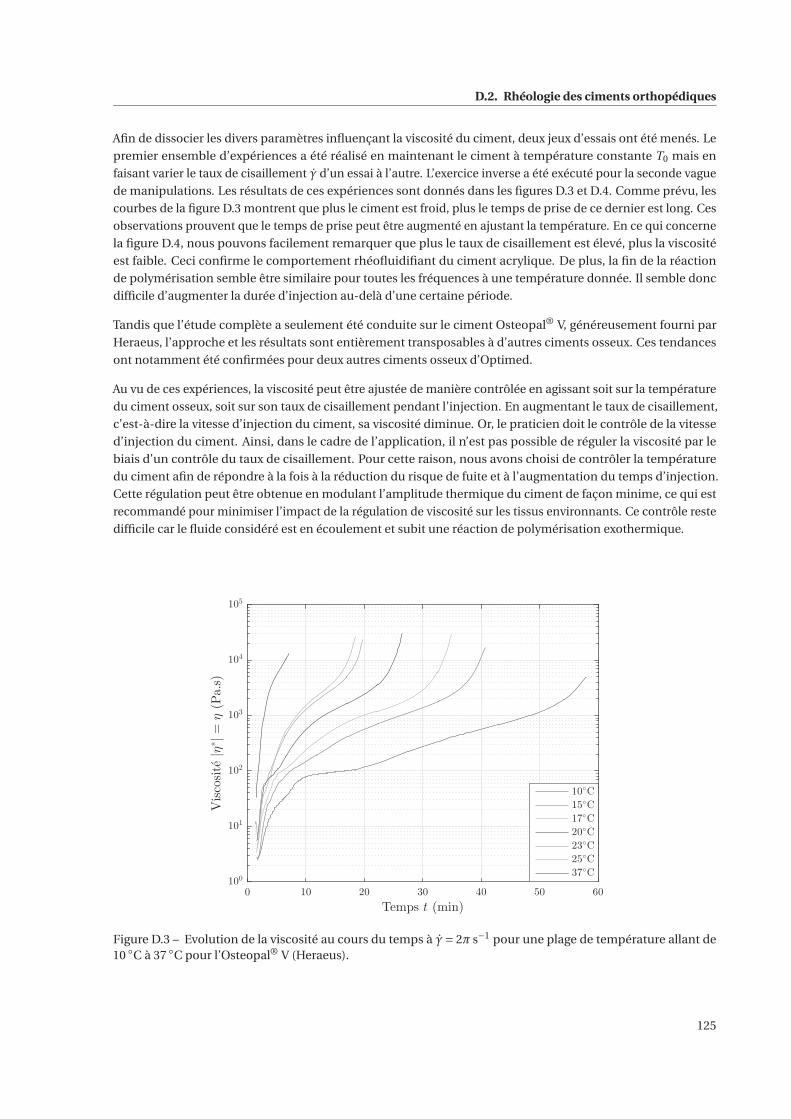
D.2. Rhéologie des ciments orthopédiques
Afin de dissocier les divers paramètres influençant la viscosité du ciment, deux jeux d’essais ont été menés. Le
premier ensemble d’expériences a été réalisé en maintenant le ciment à température constante T0 mais en
faisant varier le taux de cisaillement γ d’un essai à l’autre. L’exercice inverse a été exécuté pour la seconde vague
de manipulations. Les résultats de ces expériences sont donnés dans les figures D.3 et D.4. Comme prévu, les
courbes de la figure D.3 montrent que plus le ciment est froid, plus le temps de prise de ce dernier est long. Ces
observations prouvent que le temps de prise peut être augmenté en ajustant la température. En ce qui concerne
la figure D.4, nous pouvons facilement remarquer que plus le taux de cisaillement est élevé, plus la viscosité
est faible. Ceci confirme le comportement rhéofluidifiant du ciment acrylique. De plus, la fin de la réaction
de polymérisation semble être similaire pour toutes les fréquences à une température donnée. Il semble donc
difficile d’augmenter la durée d’injection au-delà d’une certaine période.
Tandis que l’étude complète a seulement été conduite sur le ciment Osteopal® V, généreusement fourni par
Heraeus, l’approche et les résultats sont entièrement transposables à d’autres ciments osseux. Ces tendances
ont notamment été confirmées pour deux autres ciments osseux d’Optimed.
Au vu de ces expériences, la viscosité peut être ajustée de manière contrôlée en agissant soit sur la température
du ciment osseux, soit sur son taux de cisaillement pendant l’injection. En augmentant le taux de cisaillement,
c’est-à-dire la vitesse d’injection du ciment, sa viscosité diminue. Or, le praticien doit le contrôle de la vitesse
d’injection du ciment. Ainsi, dans le cadre de l’application, il n’est pas possible de réguler la viscosité par le
biais d’un contrôle du taux de cisaillement. Pour cette raison, nous avons choisi de contrôler la température
du ciment afin de répondre à la fois à la réduction du risque de fuite et à l’augmentation du temps d’injection.
Cette régulation peut être obtenue en modulant l’amplitude thermique du ciment de façon minime, ce qui est
recommandé pour minimiser l’impact de la régulation de viscosité sur les tissus environnants. Ce contrôle reste
difficile car le fluide considéré est en écoulement et subit une réaction de polymérisation exothermique.
0 10 20 30 40 50 60
Temps t (min)
100
101
102
103
104
105
Viscosite|η
∗|=
η(Pa.s)
10◦C
15◦C
17◦C
20◦C
23◦C
25◦C
37◦C
Figure D.3 – Evolution de la viscosité au cours du temps à γ= 2π s−1 pour une plage de température allant de10 ◦C à 37 ◦C pour l’Osteopal® V (Heraeus).
125
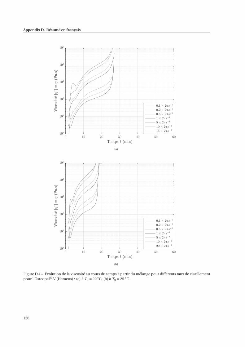
Appendix D. Résumé en français
0 10 20 30 40 50 60
Temps t (min)
100
101
102
103
104
105
Viscosite|η
∗|=
η(Pa.s)
0.1 × 2πs−1
0.2 × 2πs−1
0.5 × 2πs−1
1 × 2πs−1
5 × 2πs−1
10 × 2πs−1
15 × 2πs−1
(a)
0 10 20 30 40 50 60
Temps t (min)
100
101
102
103
104
105
Viscosite|η
∗|=
η(Pa.s)
0.1 × 2πs−1
0.2 × 2πs−1
0.5 × 2πs−1
1 × 2πs−1
5 × 2πs−1
10 × 2πs−1
20 × 2πs−1
(b)
Figure D.4 – Evolution de la viscosité au cours du temps à partir du mélange pour différents taux de cisaillementpour l’Osteopal® V (Heraeus) : (a) à T0 = 20 ◦C; (b) à T0 = 25 ◦C.
126
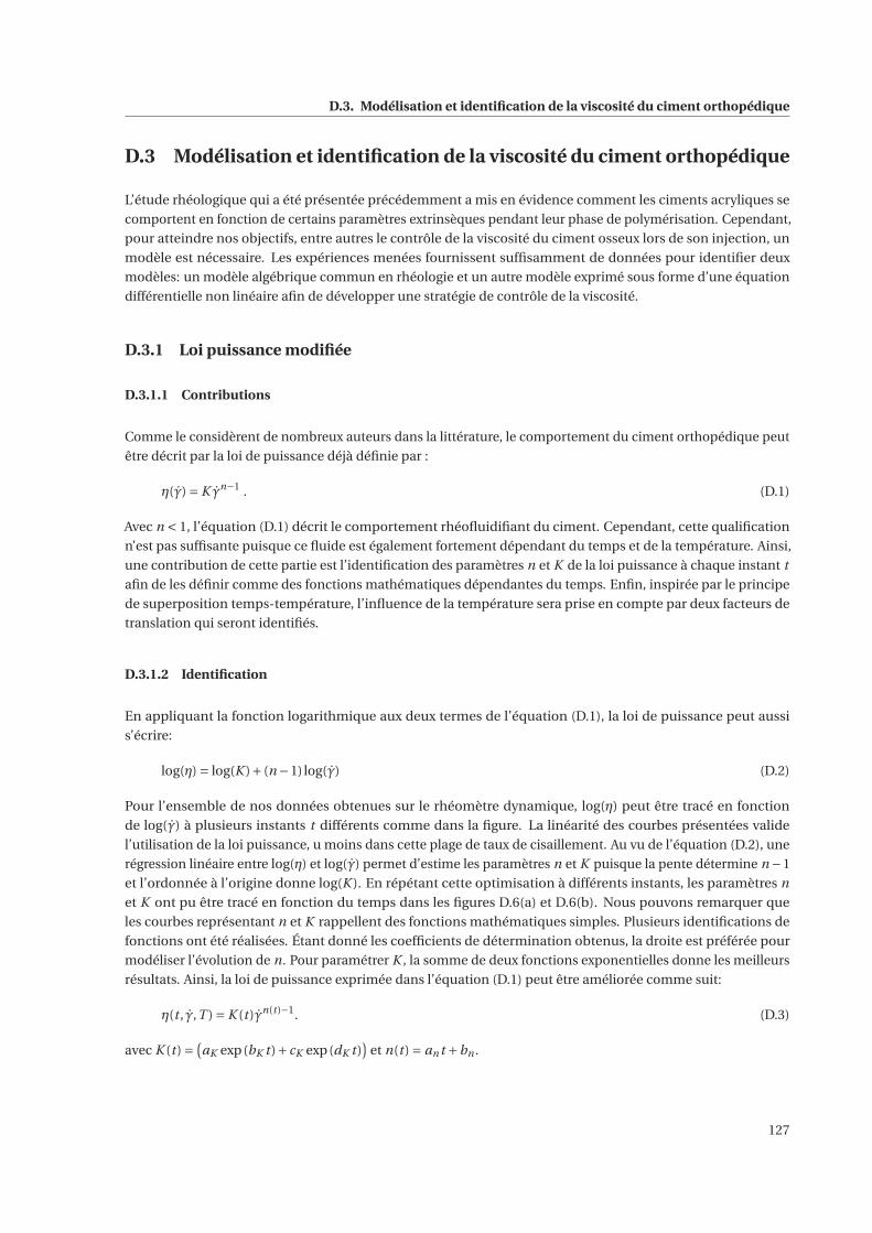
D.3. Modélisation et identification de la viscosité du ciment orthopédique
D.3 Modélisation et identification de la viscosité du ciment orthopédique
L’étude rhéologique qui a été présentée précédemment a mis en évidence comment les ciments acryliques se
comportent en fonction de certains paramètres extrinsèques pendant leur phase de polymérisation. Cependant,
pour atteindre nos objectifs, entre autres le contrôle de la viscosité du ciment osseux lors de son injection, un
modèle est nécessaire. Les expériences menées fournissent suffisamment de données pour identifier deux
modèles: un modèle algébrique commun en rhéologie et un autre modèle exprimé sous forme d’une équation
différentielle non linéaire afin de développer une stratégie de contrôle de la viscosité.
D.3.1 Loi puissance modifiée
D.3.1.1 Contributions
Comme le considèrent de nombreux auteurs dans la littérature, le comportement du ciment orthopédique peut
être décrit par la loi de puissance déjà définie par :
η(γ) = K γn−1 . (D.1)
Avec n < 1, l’équation (D.1) décrit le comportement rhéofluidifiant du ciment. Cependant, cette qualification
n’est pas suffisante puisque ce fluide est également fortement dépendant du temps et de la température. Ainsi,
une contribution de cette partie est l’identification des paramètres n et K de la loi puissance à chaque instant t
afin de les définir comme des fonctions mathématiques dépendantes du temps. Enfin, inspirée par le principe
de superposition temps-température, l’influence de la température sera prise en compte par deux facteurs de
translation qui seront identifiés.
D.3.1.2 Identification
En appliquant la fonction logarithmique aux deux termes de l’équation (D.1), la loi de puissance peut aussi
s’écrire:
log(η) = log(K )+ (n −1)log(γ) (D.2)
Pour l’ensemble de nos données obtenues sur le rhéomètre dynamique, log(η) peut être tracé en fonction
de log(γ) à plusieurs instants t différents comme dans la figure. La linéarité des courbes présentées valide
l’utilisation de la loi puissance, u moins dans cette plage de taux de cisaillement. Au vu de l’équation (D.2), une
régression linéaire entre log(η) et log(γ) permet d’estime les paramètres n et K puisque la pente détermine n −1
et l’ordonnée à l’origine donne log(K ). En répétant cette optimisation à différents instants, les paramètres n
et K ont pu être tracé en fonction du temps dans les figures D.6(a) et D.6(b). Nous pouvons remarquer que
les courbes représentant n et K rappellent des fonctions mathématiques simples. Plusieurs identifications de
fonctions ont été réalisées. Étant donné les coefficients de détermination obtenus, la droite est préférée pour
modéliser l’évolution de n. Pour paramétrer K , la somme de deux fonctions exponentielles donne les meilleurs
résultats. Ainsi, la loi de puissance exprimée dans l’équation (D.1) peut être améliorée comme suit:
η(t , γ,T ) = K (t )γn(t )−1. (D.3)
avec K (t ) =(aK exp(bK t )+ cK exp(dK t )
)et n(t ) = an t +bn .
127
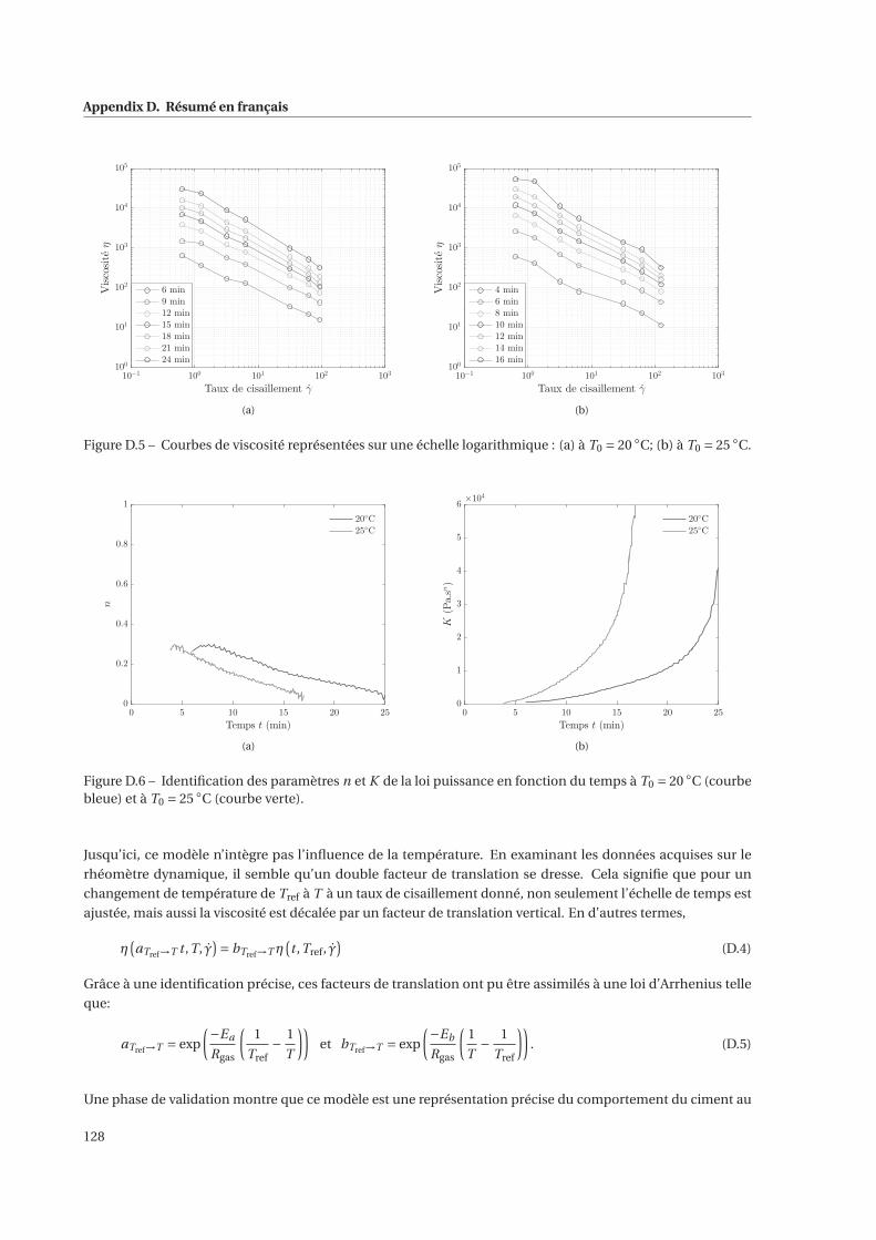
Appendix D. Résumé en français
10−1
100
101
102
103
Taux de cisaillement γ
100
101
102
103
104
105
Viscositeη
6 min
9 min
12 min
15 min
18 min
21 min
24 min
(a)
10−1
100
101
102
103
Taux de cisaillement γ
100
101
102
103
104
105
Viscositeη
4 min
6 min
8 min
10 min
12 min
14 min
16 min
(b)
Figure D.5 – Courbes de viscosité représentées sur une échelle logarithmique : (a) à T0 = 20 ◦C; (b) à T0 = 25 ◦C.
0 5 10 15 20 25
Temps t (min)
0
0.2
0.4
0.6
0.8
1
n
20◦C
25◦C
(a)
0 5 10 15 20 25
Temps t (min)
0
1
2
3
4
5
6
K(Pa.sn)
×104
20◦C
25◦C
(b)
Figure D.6 – Identification des paramètres n et K de la loi puissance en fonction du temps à T0 = 20 ◦C (courbebleue) et à T0 = 25 ◦C (courbe verte).
Jusqu’ici, ce modèle n’intègre pas l’influence de la température. En examinant les données acquises sur le
rhéomètre dynamique, il semble qu’un double facteur de translation se dresse. Cela signifie que pour un
changement de température de Tref à T à un taux de cisaillement donné, non seulement l’échelle de temps est
ajustée, mais aussi la viscosité est décalée par un facteur de translation vertical. En d’autres termes,
η(aTref→T t ,T, γ
)= bTref→T η
(t ,Tref, γ
)(D.4)
Grâce à une identification précise, ces facteurs de translation ont pu être assimilés à une loi d’Arrhenius telle
que:
aTref→T = exp
(−Ea
Rgas
(1
Tref− 1
T
))et bTref→T = exp
(−Eb
Rgas
(1
T− 1
Tref
)). (D.5)
Une phase de validation montre que ce modèle est une représentation précise du comportement du ciment au
128
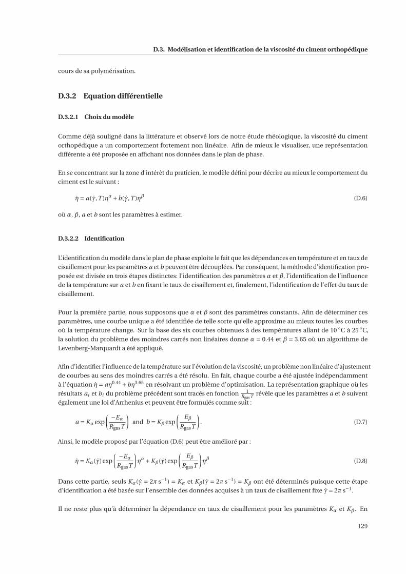
D.3. Modélisation et identification de la viscosité du ciment orthopédique
cours de sa polymérisation.
D.3.2 Equation différentielle
D.3.2.1 Choix du modèle
Comme déjà souligné dans la littérature et observé lors de notre étude rhéologique, la viscosité du ciment
orthopédique a un comportement fortement non linéaire. Afin de mieux le visualiser, une représentation
différente a été proposée en affichant nos données dans le plan de phase.
En se concentrant sur la zone d’intérêt du praticien, le modèle défini pour décrire au mieux le comportement du
ciment est le suivant :
η= a(γ,T )ηα+b(γ,T )ηβ (D.6)
où α, β, a et b sont les paramètres à estimer.
D.3.2.2 Identification
L’identification du modèle dans le plan de phase exploite le fait que les dépendances en température et en taux de
cisaillement pour les paramètres a et b peuvent être découplées. Par conséquent, la méthode d’identification pro-
posée est divisée en trois étapes distinctes: l’identification des paramètres α et β, l’identification de l’influence
de la température sur a et b en fixant le taux de cisaillement et, finalement, l’identification de l’effet du taux de
cisaillement.
Pour la première partie, nous supposons que α et β sont des paramètres constants. Afin de déterminer ces
paramètres, une courbe unique a été identifiée de telle sorte qu’elle approxime au mieux toutes les courbes
où la température change. Sur la base des six courbes obtenues à des températures allant de 10 ◦C à 25 ◦C,
la solution du problème des moindres carrés non linéaires donne α = 0.44 et β = 3.65 où un algorithme de
Levenberg-Marquardt a été appliqué.
Afin d’identifier l’influence de la température sur l’évolution de la viscosité, un problème non linéaire d’ajustement
de courbes au sens des moindres carrés a été résolu. En fait, chaque courbe a été ajustée indépendamment
à l’équation η= aη0.44 +bη3.65 en résolvant un problème d’optimisation. La représentation graphique où les
résultats ai et bi du problème précédent sont tracés en fonction 1RgasT révèle que les paramètres a et b suivent
également une loi d’Arrhenius et peuvent être formulés comme suit :
a = Kα exp
( −Eα
RgasT
)and b = Kβ exp
(Eβ
RgasT
). (D.7)
Ainsi, le modèle proposé par l’équation (D.6) peut être amélioré par :
η= Kα(γ)exp
( −Eα
RgasT
)ηα+Kβ(γ)exp
(Eβ
RgasT
)ηβ (D.8)
Dans cette partie, seuls Kα(γ = 2π s−1) = Kα et Kβ(γ = 2π s−1) = Kβ ont été déterminés puisque cette étape
d’identification a été basée sur l’ensemble des données acquises à un taux de cisaillement fixe γ= 2π s−1.
Il ne reste plus qu’à déterminer la dépendance en taux de cisaillement pour les paramètres Kα et Kβ. En
129
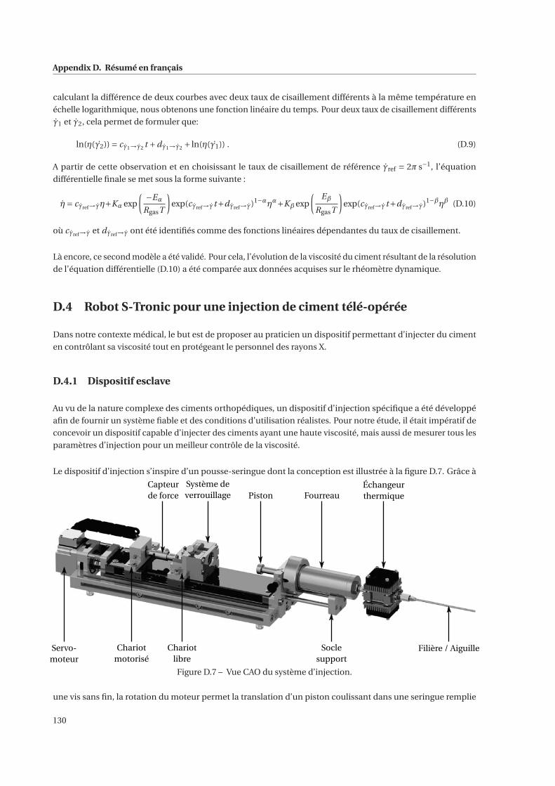
Appendix D. Résumé en français
calculant la différence de deux courbes avec deux taux de cisaillement différents à la même température en
échelle logarithmique, nous obtenons une fonction linéaire du temps. Pour deux taux de cisaillement différents
γ1 et γ2, cela permet de formuler que:
ln(η(γ2)) = cγ1→γ2 t +dγ1→γ2 + ln(η(γ1)) . (D.9)
A partir de cette observation et en choisissant le taux de cisaillement de référence γref = 2π s−1, l’équation
différentielle finale se met sous la forme suivante :
η= cγref→γη+Kα exp
( −Eα
RgasT
)exp(cγref→γt+dγref→γ)1−αηα+Kβ exp
(Eβ
RgasT
)exp(cγref→γt+dγref→γ)1−βηβ (D.10)
où cγref→γ et dγref→γ ont été identifiés comme des fonctions linéaires dépendantes du taux de cisaillement.
Là encore, ce second modèle a été validé. Pour cela, l’évolution de la viscosité du ciment résultant de la résolution
de l’équation différentielle (D.10) a été comparée aux données acquises sur le rhéomètre dynamique.
D.4 Robot S-Tronic pour une injection de ciment télé-opérée
Dans notre contexte médical, le but est de proposer au praticien un dispositif permettant d’injecter du ciment
en contrôlant sa viscosité tout en protégeant le personnel des rayons X.
D.4.1 Dispositif esclave
Au vu de la nature complexe des ciments orthopédiques, un dispositif d’injection spécifique a été développé
afin de fournir un système fiable et des conditions d’utilisation réalistes. Pour notre étude, il était impératif de
concevoir un dispositif capable d’injecter des ciments ayant une haute viscosité, mais aussi de mesurer tous les
paramètres d’injection pour un meilleur contrôle de la viscosité.
Le dispositif d’injection s’inspire d’un pousse-seringue dont la conception est illustrée à la figure D.7. Grâce à
PistonSystème deverrouillage
Filière / AiguilleChariotmotorisé
Échangeurthermique
Capteurde force
Servo-moteur
Chariotlibre
Fourreau
Soclesupport
Figure D.7 – Vue CAO du système d’injection.
une vis sans fin, la rotation du moteur permet la translation d’un piston coulissant dans une seringue remplie
130
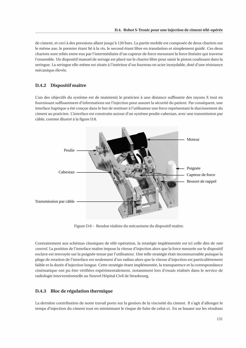
D.4. Robot S-Tronic pour une injection de ciment télé-opérée
de ciment, et ceci à des pressions allant jusqu’à 120 bars. La partie mobile est composée de deux chariots sur
le même axe, le premier étant lié à la vis, le second étant libre en translation et simplement guidé. Ces deux
chariots sont reliés entre eux par l’intermédiaire d’un capteur de force mesurant la force linéaire qui traverse
l’ensemble. Un dispositif manuel de serrage est placé sur le chariot libre pour saisir le piston coulissant dans la
seringue. La seringue elle-même est située à l’intérieur d’un fourreau en acier inoxydable, doté d’une résistance
mécanique élevée.
D.4.2 Dispositif maître
L’un des objectifs du système est de maintenir le praticien à une distance suffisante des rayons X tout en
fournissant suffisamment d’informations sur l’injection pour assurer la sécurité du patient. Par conséquent, une
interface haptique a été conçue dans le but de restituer à l’utilisateur une force représentant le durcissement du
ciment au praticien. L’interface est construite autour d’un système poulie-cabestan, avec une transmission par
câble, comme illustré à la figure D.8.
Moteur
Poignée
Capteur de force
Ressort de rappel
Poulie
Cabestan
Transmission par câble
Figure D.8 – Rendue réaliste du mécanisme du dispositif maître.
Contrairement aux schémas classiques de télé-opération, la stratégie implémentée est ici celle dite de rate
control. La position de l’interface maître impose la vitesse d’injection alors que la force mesurée sur le dispositif
esclave est renvoyée sur la poignée tenue par l’utilisateur. Une telle stratégie était incontournable puisque la
plage de rotation de l’interface est seulement d’un radian alors que la vitesse d’injection est particulièrement
faible et la durée d’injection longue. Cette stratégie étant implémentée, la transparence et la correspondance
cinématique ont pu être vérifiées expérimentalement, notamment lors d’essais réalisés dans le service de
radiologie interventionnelle au Nouvel Hôpital Civil de Strasbourg.
D.4.3 Bloc de régulation thermique
La dernière contribution de notre travail porte sur la gestion de la viscosité du ciment. Il s’agit d’allonger le
temps d’injection du ciment tout en minimisant le risque de fuite de celui-ci. En se basant sur les résultats
131
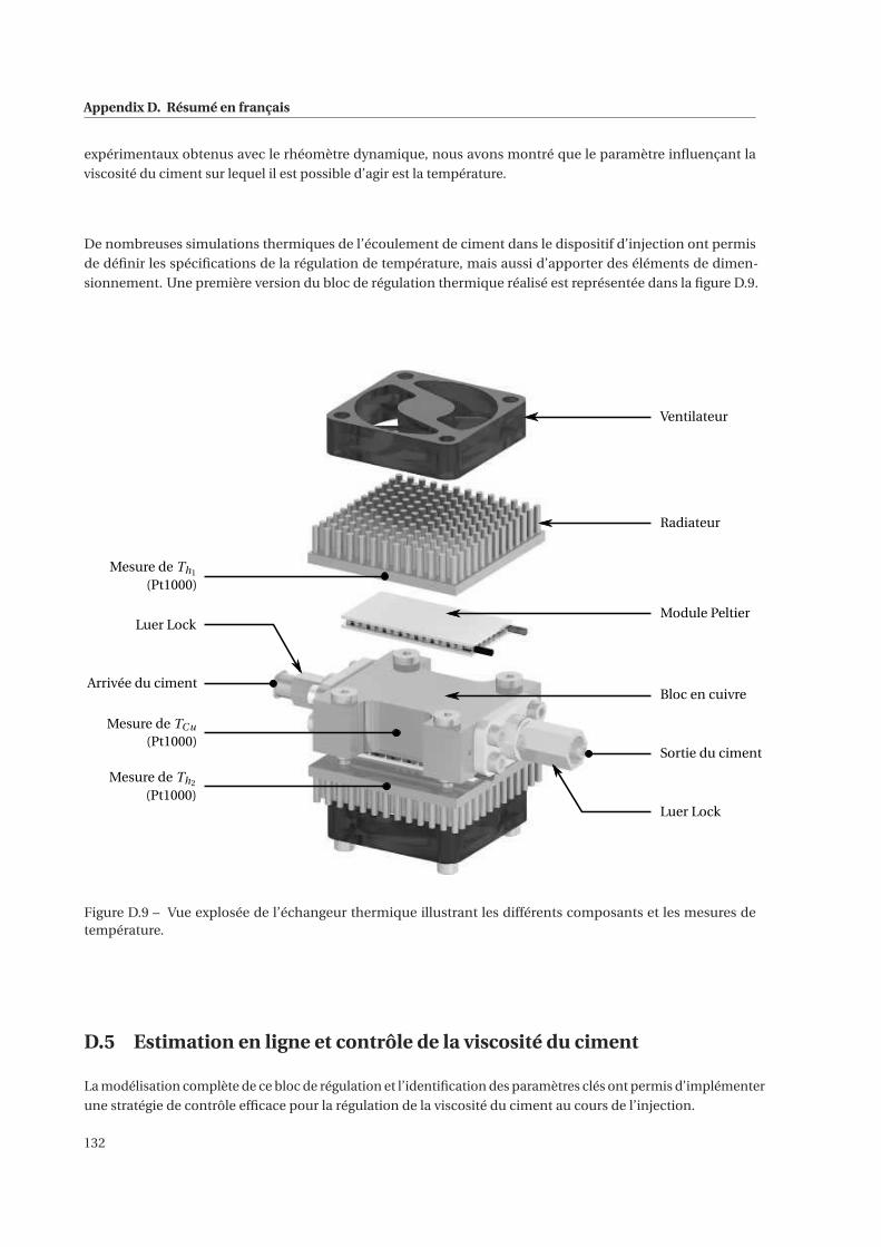
Appendix D. Résumé en français
expérimentaux obtenus avec le rhéomètre dynamique, nous avons montré que le paramètre influençant la
viscosité du ciment sur lequel il est possible d’agir est la température.
De nombreuses simulations thermiques de l’écoulement de ciment dans le dispositif d’injection ont permis
de définir les spécifications de la régulation de température, mais aussi d’apporter des éléments de dimen-
sionnement. Une première version du bloc de régulation thermique réalisé est représentée dans la figure D.9.
Ventilateur
Radiateur
Module Peltier
Bloc en cuivre
Luer Lock
Sortie du ciment
Mesure de Th1
(Pt1000)
Arrivée du ciment
Luer Lock
Mesure de TCu
(Pt1000)
Mesure de Th2
(Pt1000)
Figure D.9 – Vue explosée de l’échangeur thermique illustrant les différents composants et les mesures detempérature.
D.5 Estimation en ligne et contrôle de la viscosité du ciment
La modélisation complète de ce bloc de régulation et l’identification des paramètres clés ont permis d’implémenter
une stratégie de contrôle efficace pour la régulation de la viscosité du ciment au cours de l’injection.
132
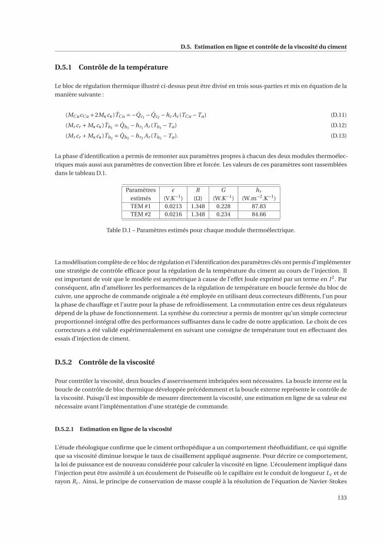
D.5. Estimation en ligne et contrôle de la viscosité du ciment
D.5.1 Contrôle de la température
Le bloc de régulation thermique illustré ci-dessus peut être divisé en trois sous-parties et mis en équation de la
manière suivante :
(MCucCu +2Mκcκ)TCu =−Qc1 −Qc2 −hc Ac (TCu −Ta) (D.11)
(Mr cr +Mκcκ)Th1 = Qh1 −hr1 Ar (Th1 −Ta) (D.12)
(Mr cr +Mκcκ)Th2 = Qh2 −hr2 Ar (Th2 −Ta). (D.13)
La phase d’identification a permis de remonter aux paramètres propres à chacun des deux modules thermoélec-
triques mais aussi aux paramètres de convection libre et forcée. Les valeurs de ces paramètres sont rassemblées
dans le tableau D.1.
Paramètres ε R G hr
estimés (V.K−1) (Ω) (W.K−1) (W.m−2.K−1)TEM #1 0.0213 1.348 0.228 87.83TEM #2 0.0216 1.348 0.234 84.66
Table D.1 – Paramètres estimés pour chaque module thermoélectrique.
La modélisation complète de ce bloc de régulation et l’identification des paramètres clés ont permis d’implémenter
une stratégie de contrôle efficace pour la régulation de la température du ciment au cours de l’injection. Il
est important de voir que le modèle est asymétrique à cause de l’effet Joule exprimé par un terme en I 2. Par
conséquent, afin d’améliorer les performances de la régulation de température en boucle fermée du bloc de
cuivre, une approche de commande originale a été employée en utilisant deux correcteurs différents, l’un pour
la phase de chauffage et l’autre pour la phase de refroidissement. La commutation entre ces deux régulateurs
dépend de la phase de fonctionnement. La synthèse du correcteur a permis de montrer qu’un simple correcteur
proportionnel-intégral offre des performances suffisantes dans le cadre de notre application. Le choix de ces
correcteurs a été validé expérimentalement en suivant une consigne de température tout en effectuant des
essais d’injection de ciment.
D.5.2 Contrôle de la viscosité
Pour contrôler la viscosité, deux boucles d’asservissement imbriquées sont nécessaires. La boucle interne est la
boucle de contrôle de bloc thermique développée précédemment et la boucle externe représente le contrôle de
la viscosité. Puisqu’il est impossible de mesurer directement la viscosité, une estimation en ligne de sa valeur est
nécessaire avant l’implémentation d’une stratégie de commande.
D.5.2.1 Estimation en ligne de la viscosité
L’étude rhéologique confirme que le ciment orthopédique a un comportement rhéofluidifiant, ce qui signifie
que sa viscosité diminue lorsque le taux de cisaillement appliqué augmente. Pour décrire ce comportement,
la loi de puissance est de nouveau considérée pour calculer la viscosité en ligne. L’écoulement impliqué dans
l’injection peut être assimilé à un écoulement de Poiseuille où le capillaire est le conduit de longueur Lc et de
rayon Rc . Ainsi, le principe de conservation de masse couplé à la résolution de l’équation de Navier-Stokes
133
Appendix D. Résumé en français
fournit la relation suivante entre la perte de charge ΔP et le débit Q :
Q =(ΔP
Lc
) 1n(
Rc
2K
) 1n(πnR3
c
3n +1
)(D.14)
Afin de calculer en ligne la viscosité du ciment, une instrumentation adaptée a été ajoutée au dispositif
d’injection. Le capteur de force dans la transmission fournit une mesure de la force d’injection qui permet à
son tour d’évaluer ΔP alors que le capteur de position permet de calculer le débit Q. Ensuite, l’indice n de la loi
puissance est supposé être connu, ici constant et égal à 0.2. Avec cette dernière hypothèse, l’équation (D.14)
permet d’estimer la valeur de K au cours de l’injection. Enfin, pour reconstruire la valeur de la viscosité, le taux
de cisaillement est calculé puis la loi puissance appliquée.
L’estimation en ligne de la viscosité a été implémentée puis expérimentée à plusieurs reprises au cours d’injection
avec le système esclave en utilisant du ciment Osteopal® V de Heraeus. Les résultats de ces manipulations ont
été comparés au modèle que nous avions identifié grâce à l’étude rhéologique. Cela permet de valider notre
estimation de viscosité en ligne.
D.5.2.2 Contrôle de la viscosité
A partir de cette estimation de viscosité en ligne qui a été validée, le contrôle de la viscosité du ciment osseux
peut être considéré. En prenant en compte les remarques des praticiens, la consigne optimale de viscosité serait
une valeur constante, définie de telle sorte que les fuites de ciment osseux soient limitées et que l’écoulement
de ciment à l’intérieur de la vertèbre traitée reste homogène. Avec une telle référence, le praticien pourrait
idéalement prendre autant de temps que nécessaire pour effectuer l’injection. En pratique, une telle consigne ne
peut pas être suivie puisque la réaction de polymérisation qui en cours ne peut pas être arrêtée et est irréversible.
Néanmoins, cette idée a été mise en œuvre. Dans ce cas, la conception d’un correcteur de viscosité spécifique
n’est pas nécessaire puisque la génération de la consigne de température T ∗Cu est alors limitée à du tout ou
rien. En effet, le ciment osseux doit être chauffé jusqu’à ce que sa viscosité atteigne la consigne de viscosité
donnée, puis refroidi afin de ralentir la réaction de polymérisation et donc d’augmenter le temps d’injection.
Les premières expériences qui considèrent cette consigne de viscosité sont concluantes.
Ensuite, une consigne de viscosité plus complexe a été considérée. Alors que des résultats de simulations
montrent que ce contrôle de viscosité est très prometteur, des résultats identiques n’ont pas encore été obtenus
en ligne.
D.6 Conclusions
Ce travail de thèse a permis, dans un premier temps, de caractériser l’évolution de la viscosité du ciment
orthopédique au cours du temps mais aussi en fonction de la température et du taux de cisaillement. Cette
caractérisation a abouti à deux modèles et à leur identification. Ensuite, pour répondre à la problématique de
protection du praticien, un système d’injection télé-opérée avec retour d’effort a été conçu. Celui-ci permet
également de réguler la viscosité du ciment grâce au contrôle précis de sa température. Cette fonctionnalité
permet de limiter le risque de fuite, tout en allongeant le temps d’injection, rendant ainsi l’intervention de
vertébroplastie plus aisée.
Ce travail, effectué dans le cadre d’un projet financé par la SATT Conectus, a conduit à un prototype fonctionnel
avec lequel des essais d’injection dans des vertèbres fantômes ont été réalisés par des praticiens au service de
Radiologie Interventionnelle du NHC.
134
References
[Al-Hadithi 1992] T. S. R. Al-Hadithi, H. A. Barnes and K. Walters. The relationship between the linear (oscillatory)
and nonlinear (steady-state) flow properties of a series of polymer and colloidal systems. Colloid and
Polymer Science, vol. 270, no. 1, pages 40–46, 1992. (cited page 36)
[AnatomyExpert 2016] AnatomyExpert. http://www.anatomyexpert.com/, 2016. (cited pages xiii and 3)
[Anselmetti 2007] G. C. Anselmetti, G. Corrao, P. Della Monica, V. Tartaglia, A. Manca, H. Eminefendic, F. Russo,
I. Tosetti and D. Regge. Pain Relief Following Percutaneous Vertebroplasty: Results of a Series of 283
Consecutive Patients Treated in a Single Institution. CardioVascular and Interventional Radiology, vol. 30,
no. 3, pages 441–447, June 2007. (cited page 16)
[ARDES 2014] ARDES. http://www.ardes-group.com/fr/blog/produit/seringue-10cc/, 2014. (cited pages xiv
and 63)
[ATIH 2016] Agence Technique de l’Information sur l’Hospitalisation ATIH. Formulaire d’interrogation des
données. http://www.scansante.fr/applications/statistiques-activite-MCO-par-GHM, 2016. (cited pages
xiii and 9)
[Barnes 1989] H. A. Barnes, J. F. Hutton and K. Walters. An introduction to rheology, volume 3. Elsevier, 1989.
(cited page 24)
[Baroud 2003] G. Baroud, J. Z. Wu, M. Bohner, S. Sponagel and T. Steffen. How to determine the permeability for
cement infiltration of osteoporotic cancellous bone. Medical Engineering & Physics, vol. 25, no. 4, pages
283–288, 2003. (cited page 32)
[Baroud 2004a] G. Baroud, M. Samara and T. Steffen. Influence of Mixing Method on the Cement Temperature-
Mixing Time History and Doughing Time of Three Acrylic Cements for Vertebroplasty. Journal of Biomedical
Materials Research Part B: Applied Biomaterials, vol. 68B, no. 1, pages 112–116, January 2004. (cited pages
14 and 31)
[Baroud 2004b] G. Baroud and F. B. Yahia. A finite element rheological model for polymethylmethacrylate flow:
Analysis of the cement delivery in vertebroplasty. Proceedings of the Institution of Mechanical Engineers,
Part H: Journal of Engineering in Medicine, vol. 218, no. 5, pages 331–338, Mai 2004. (cited page 33)
[Baroud 2006] G. Baroud, M. Crookshank and M. Bohner. High-Viscosity Cement Significantly Enhances Unifor-
mity of Cement Filling in Vertebroplasty: An Experimental Model and Study on Cement Leakage. Spine,
vol. 31, pages 2562–2568, 2006. (cited page 33)
[Baroud 2013a] G. Baroud. Bone cement delivery system, US 20130123790 A1 2013. (cited page 20)
135
References
[Baroud 2013b] G. Baroud. Integrated cement delivery system for bone augmentation procedures and methods,
US 20130190680 A1 2013. (cited page 20)
[Baroud 2014] G. Baroud. Method and Apparatus for Monitoring and/or Controlling the Curing of Cements used
in Medical Procedures , US 20140009173 A1 2014. (cited page 20)
[Barr 2000] J. D. Barr, M. S. Barr, T. J. Lemley and R. M. McCann. Percutaneous vertebroplasty for pain relief and
spinal stabilization. Spine, vol. 25, no. 8, pages 923–928, 2000. (cited page 16)
[Bayle 2013] B. Bayle and L. Barbé. Tele-manipulation, chapter 8, pages 269–302. John Wiley & Sons, Inc., 2013.
(cited pages xv, 75, and 76)
[Bird 1987] R. Byron Bird, R. C. Amstrong and O. Assager. Dynamics of Polymeric Liquids, Volume 1: Fluid
Mechanics. A Wiley-Interscience Publication, John Wiley & Sons, 1987. (cited pages 24, 33, 35, and 42)
[Boger 2009] A. Boger, K. Wheeler, B. Schenk and P. Heini. Clinical investigations of polymethylmethacrylate
cement viscosity during vertebroplasty and related in vitro measurements. European Spine Journal, vol. 18,
pages 1272–1278, 2009. (cited pages 33 and 111)
[Bohner 2003] M. Bohner, B. Gasser, Baroud G. and P. Heini. Theoretical and experimental model to describe
the injection of a polymethylmethacrylate cement into a porous structure. Biomat, vol. 24, no. 16, pages
2721–2730, July 2003. (cited pages 31 and 33)
[Burge 2007] R. Burge, B. Dawson-Hughes, D. H. Solomon, J. B. Wong, A. King and A. Tosteson. Incidence and
economic burden of osteoporosis-related fractures in the United States, 2005–2025. Journal of Bone and
Mineral Research, vol. 22, no. 3, pages 465–475, 2007. (cited page 5)
[CareFusion 2016] CareFusion. AVAmax® Advanced Vertebral Augmentation system. http://www.carefusion.
com/documents/brochures/interventional-specialties/IS_AVAmax-Vertebral-Augmentation-System_
BR_EN.pdf, 2016. (cited page 18)
[Carreau 1972] P. J. Carreau. Rheological Equations from Molecular Network Theories. Transactions of The
Society of Rheology (1957-1977), vol. 16, pages 99–127, January 1972. (cited page 33)
[Center 2015] Garden State Medical Center. Kyphoplasty/Vertebroplasty. http://gsmedicalcenter.org/services/
pain-management/minimally-invasive-procedures/kyphoplasty-vertebroplasty/, 2015. (cited pages xiii
and 7)
[Chang 2015] X. Chang, Y.-F. Lv, B. Chen, H.-y. Li, X.-b. Han, K. Yang, W. Zhang, Y. Zhou and C.-q. Li. Vertebro-
plasty versus kyphoplasty in osteoporotic vertebral compression fracture: a meta-analysis of prospective
comparative studies. International Orthopaedics, vol. 39, no. 3, pages 491–500, March 2015. (cited page 7)
[Charnley 1972] J. Charnley. The long-term results of low-friction arthroplasty of the hip performed as a primary
intervention. Bone & Joint Journal, vol. 54, no. 1, pages 61–76, 1972. (cited page 9)
[Chavali 2003] R. Chavali, R. Resijek, S. K. Knight and I. Choi. Extending Polymerization Time of Polymethyl-
methacrylate Cement in Percutaneous Vertebroplasty with Ice Bath Cooling. American Journal of Neurora-
diology, vol. 24, no. 3, pages 545–546, 2003. (cited page 64)
[Choi 2007] H.-S. Choi, S. Yun and K.-i. Whang. Development of a temperature-controlled car-seat system
utilizing thermoelectric device. Applied Thermal Engineering, vol. 27, no. 17–18, pages 2841–2849, 2007.
(cited page 70)
[Cox 1958] W. P. Cox and E. H. Merz. Correlation of dynamic and steady flow viscosities. Journal of Polymer
Science, vol. 28, pages 619–622, April 1958. (cited page 35)
136
References
[Dealy 2006] J. M. Dealy and R. G. Larson. Structure and rheology of molten polymers. Carl Hanser Verlag
GmbH & Co. KG, 2006. (cited pages 33, 35, 42, and 45)
[Deramond 1998] H. Deramond, C. Depriester, P. Galibert and D. Le Gars. Percutaneous vertebroplasty with
polymethylmethacrylate. Technique, indications, and results. Radiologic Clinics of North America, vol. 36,
pages 533–546, May 1998. (cited page 8)
[DFine 2016] DFine. StabiliT®, A full family of VCF solutions to match the unique needs of every patient.
http://dfineinc.com/stabilit/, 2016. (cited pages xiii, 19, and 20)
[Diamond 2004] T. H. Diamond, J. Bucci, J. H. Kersley, P. Aslan, W. B. Lynch and C. Bryant. Osteoporosis and
spinal fractures in men with prostate cancer: risk factors and effects of androgen deprivation therapy.
Journal of Urology, vol. 172, no. 2, pages 529–532, 2004. (cited page 5)
[Dunne 2001] N.J. Dunne and J.F. Orr. Influence of mixing techniques on the physical properties of acrylic bone
cement. Biomaterials, vol. 22, no. 13, pages 1819–1826, 2001. (cited page 98)
[Eck 2008] J. C. Eck, D. Nachtigall, S. C. Humphreys and S. D. Hodges. Comparison of vertebroplasty and balloon
kyphoplasty for treatment of vertebral compression fractures: a meta-analysis of the literature. The Spine
Journal, vol. 8, no. 3, pages 488–497, June 2008. (cited pages 7 and 16)
[Esarte 2001] J. Esarte, G. Min and D. M. Rowe. Modelling heat exchangers for thermoelectric generators. Journal
of Power Sources, vol. 93, no. 1–2, pages 72–76, 2001. (cited page 70)
[Fang 2009] S.-C. Fang and H.-L. Chan. Human identification by quantifying similarity and dissimilarity in
electrocardiogram phase space. Pattern Recognition, vol. 42, no. 9, pages 1824–1831, 2009. (cited page 52)
[Farrar 2001] D. F. Farrar and J. Rose. Rheological properties of PMMA bone cements during curing. Biomaterials,
vol. 22, no. 22, pages 3005–3013, 2001. (cited pages 30 and 33)
[Felsenberg 2002] D. Felsenberg, A. J. Silman, M. Lunt, G. Armbrecht, A. A. Ismail, J. D. Finn, W. C. Cockerill,
D. Banzer, L. I. Benevolenskaya, A. Bhalla et al. Incidence of Vertebral Fracture in Europe: Results From the
European Prospective Osteoporosis Study (EPOS). Journal of Bone and Mineral Research, vol. 17, no. 4,
pages 716–724, 2002. (cited page 5)
[Ferreyro 2015] R. H. I. Ferreyro and M. M. Miranda. Hydraulic device for the injection of bone cement in
percutaneous vertebroplasty, US 9186194 B2 2015. (cited page 19)
[Fournier 1996] J. Fournier, G. Williams, C. Duch and G. A. Aldridge. Changes in molecular dynamics dur-
ing bulk polymerization of an epoxide-amine system as studied by dielectric relaxation spectroscopy.
Macromolecules, vol. 29, no. 22, pages 7097–7107, 1996. (cited page 33)
[Galibert 1987] P. Galibert, H. Deramond, P. Rosat and D. Le Gars. Preliminary note on the treatment of vertebral
angioma by percutaneous acrylic vertebroplasty. Neurochirurgie, vol. 33, pages 166–168, 1987. (cited
pages 6 and 8)
[Gangi 1994] A. Gangi, B. A. Kastler and J.-L. Dietemann. Percutaneous Vertebroplasty Guided by a Combination
of CT and Fluoroscopy. American Journal of Neuroradiology, vol. 15, no. 1, pages 83–86, January 1994.
(cited pages 6 and 13)
[Gangi 2006] A. Gangi, T. Sabharwal, F. G. Irani, X. Buy, J. P. Morales and A. Adam. Quality assurance guidelines for
percutaneous vertebroplasty. Cardiovascular and Interventional Radiology, vol. 29, no. 2, pages 173–178,
2006. (cited pages 5 and 14)
[Gangi 2010] A. Gangi and W. A. Clark. Have Recent Vertebroplasty Trials Changed the Indications for Vertebro-
plasty? CardioVascular and Interventional Radiology, vol. 33, no. 4, pages 677–680, June 2010. (cited page
13)
137
References
[Goldsmid 1986] H. J. Goldsmid. Electronic refrigeration. Pion, London, 1986. (cited page 85)
[Guth 2016] S. Guth and A. Gangi. Interventional Radiology Site : Patient positioning. http://www.openradiology.
org/survey/vertebroplasty/fluoroscopy/Patient%20positioning, 2016. (cited pages xiii and 13)
[Haboush 1953] E. J. Haboush. A new operation for arthroplasty of the hip based on biomechanics, photoelasticity,
fast-setting dental acrylic, and other considerations. Bulletin of the Hospital for Joint Diseases, vol. 14,
no. 2, pages 242–277, 1953. (cited page 9)
[Hagen 1839] G. H. L. Hagen. Ueber die Bewegung des Wassers in engen cylidrischen Rohren. Annalen der Physik,
vol. 46, pages 423–442, 1839. (cited page 26)
[Hannaford 1989] B. Hannaford. A design framework for teleoperators with kinesthetic feedback. IEEE Transac-
tions on Robotics and Automation, vol. 5, no. 4, pages 426–434, Aug 1989. (cited page 76)
[Harstall 2005] R. Harstall, P. F. Heini, R. L. Mini and R. Orler. Radiation Exposure to the Surgeon During
Fluoroscopically Assisted Percutaneous Vertebroplasty: A Prospective Study. Spine, vol. 30, no. 16, pages
1893–1898, 2005. (cited page 17)
[HAS 2009] HAS. Spondyloplastie par ballonets (Cyphoplastie) - Rapport d’évaluation. Rapport technique, Haute
Autorité de Santé, January 2009. (cited page 5)
[Hashtrudi-Zaad 1999] K. Hashtrudi-Zaad and S. E. Salcudean. On the use of local force feedback for transparent
teleoperation. In Robotics and Automation, 1999. Proceedings. 1999 IEEE International Conference on,
volume 3, pages 1863–1869, 1999. (cited page 76)
[Hashtrudi-Zaad 2000] K. Hashtrudi-Zaad. Design, implementation and evaluation of stable bilateral teleopera-
tion control architectures for enhanced telepresence. PhD thesis, University of British Columbia, Canada,
2000. (cited page 76)
[Heini 2000] F. P. Heini, B. Wälchli and U. Berlemann. Percutaneous transpedicular vertebroplasty with PMMA:
operative technique and early results. European Spine Journal, vol. 9, no. 5, pages 445–450, 2000. (cited
page 16)
[Hernández 2006] L. Hernández, M. Gurruchaga and I. Goñi. Influence of powder particle size distribution on
complex viscosity and other properties of acrylic bone cement for vertebroplasty and kyphoplasty. Journal
of Biomedical Materials Research Part B: Applied Biomaterials, vol. 77B, no. 1, pages 98–103, April 2006.
(cited page 31)
[Hide 2004] I. G Hide and A. Gangi. Percutaneous vertebroplasty: history, technique and current perspectives.
Clinical Radiology, vol. 59, no. 6, pages 461–467, 2004. (cited pages xiii, 13, and 16)
[Huang 2000a] B. J. Huang, C. J. Chin and C. L. Duang. A design method of thermoelectric cooler. International
Journal of Refrigeration, vol. 23, no. 3, pages 208–218, 2000. (cited page 85)
[Huang 2000b] B. J. Huang and C. L. Duang. System dynamic model and temperature control of a thermoelectric
cooler. International Journal of Refrigeration, vol. 23, no. 3, pages 197–207, 2000. (cited page 84)
[Hulme 2006] P. A. Hulme, J. Krebs, S. J. Ferguson and U. Berlemann. Vertebroplasty and kyphoplasty: a
systematic review of 69 clinical studies. Spine, vol. 31, no. 17, pages 1983–2001, 2006. (cited pages 7, 8,
and 16)
[IOF 2010] International Osteoporosis Foundation IOF. The Breaking Spine: An IOF Report. https://www.
iofbonehealth.org/sites/default/files/PDFs/WOD%20Reports/2010_the_breaking_spine_en.pdf, 2010.
(cited page 5)
138
References
[ISO 2002] International Organization for Standardization ISO. ISO 5833:2002 Implants for surgery – Acrylic
resin cements, May 2002. (cited pages 11, 14, 97, and 111)
[Jensen 1997] M. E. Jensen, A. J. Evans, J. M. Mathis, D. F. Kallmes, H. J. Cloft and J. E. Dion. Percutaneous poly-
methylmethacrylate vertebroplasty in the treatment of osteoporotic vertebral body compression fractures:
technical aspects. American Journal of Neuroradiology, vol. 18, no. 10, pages 1897–1904, 1997. (cited page
8)
[Johnell 2006] O. Johnell and J. A. Kanis. An estimate of the worldwide prevalence and disability associated with
osteoporotic fractures. Osteoporosis International, vol. 17, no. 12, pages 1726–1733, 2006. (cited page 5)
[Kanis 2013] J. A. Kanis, E. V. McCloskey, H. Johansson, C. Cooper, R. Rizzoli, J.-Y. Reginster et al. European
guidance for the diagnosis and management of osteoporosis in postmenopausal women. Osteoporosis
international, vol. 24, no. 1, pages 23–57, January 2013. (cited page 5)
[Kühn 2013] K.-D. Kühn. PMMA Cements. Springer Berlin, 2013. (cited pages 10 and 98)
[Kim 1987] W. S. Kim, F. Tendick, S. R. Ellis and L. W. Stark. A comparison of position and rate control for
telemanipulations with consideration of manipulator system dynamics. Robotics and Automation, IEEE
Journal of, vol. 3, no. 5, pages 426–436, October 1987. (cited page 77)
[Klazen 2010] C. A. H. Klazen, P. N. M. Lohle, J. de Vries, F. H. Jansen et al. Vertebroplasty versus conservative
treatment in acute osteoporotic vertebral compression fractures (Vertos II): an open-label randomised trial.
The Lancet, vol. 376, no. 9746, pages 1085–1092, 2010. (cited pages 6 and 16)
[Kolmeder 2010] S. Kolmeder and A. Lion. On the thermomechanical-chemically coupled behavior of acrylic
bone cements: experimental characterization of material behavior and modeling approach. Technische
Mechanik, vol. 30, no. 1-3, pages 195–202, 2010. (cited pages 33 and 70)
[Kolmeder 2011] S. Kolmeder, A. Lion, R. Landgraf and J. Ihlemann. Thermophysical properties and material
modelling of acrylic bone cements used in vertebroplasty. Journal of Thermal Analysis and Calorimetry,
vol. 105, pages 705–718, August 2011. (cited pages 30, 33, 50, 53, 89, and 120)
[Kolmeder 2013] S. Kolmeder and A. Lion. Characterisation and modelling rheological properties of acrylic bone
cement during application. Mechanics Research Communications, vol. 48, pages 93–99, March 2013.
(cited pages 33 and 34)
[Krause 1982] W. R. Krause, J. Miller and P. Ng. The viscosity of acrylic bone cements. Journal of Biomedical
Materials Research, vol. 16, no. 3, pages 219–243, 1982. (cited pages 30 and 32)
[Landgraf 2015] R. Landgraf, J. Ihlemann, S. Kolmeder, A. Lion, H. Lebsack and C. Kober. Modelling and
simulation of acrylic bone cement injection and curing within the framework of vertebroplasty. ZAMM -
Journal of Applied Mathematics and Mechanics / Zeitschrift für Angewandte Mathematik und Mechanik,
vol. 95, no. 12, pages 1530–1547, December 2015. (cited page 34)
[Lawrence 1993] D. A. Lawrence. Stability and transparency in bilateral teleoperation. IEEE Transactions on
Robotics and Automation, vol. 9, no. 5, pages 624–637, 1993. (cited page 76)
[Lawrence 1997] P. D. Lawrence, S. E. Salcudean, N. Sepehri, D. Chan, S. Bachmann, N. Parker, M. Zhu and
R. Frenette. Coordinated and force-feedback control of hydraulic excavators, pages 181–194. Springer
Berlin Heidelberg, Berlin, Heidelberg, 1997. (cited page 77)
[Lewis 2002] G. Lewis and M. Carroll. Rheological properties of acrylic bone cement during curing and the role of
the size of the powder particles. Journal of Biomedical Materials Research, vol. 63, no. 2, pages 191–199,
2002. (cited pages 30, 31, and 36)
139
References
[Lewis 2011] G. Lewis. Viscoelastic properties of injectable bone cements for orthopaedic applications: State-of-
the-art review. Journal of Biomedical Materials Research Part B: Applied Biomaterials, vol. 98B, no. 1,
pages 171–191, 2011. (cited page 30)
[Lian 2008] Z. Lian, C.-K. Chui and S.-H. Teoh. A biomechanical model for real-time simulation of PMMA
injection with haptics. Computers in Biology and Medicine, vol. 38, no. 3, pages 304–312, 2008. (cited
pages 32 and 36)
[Lineykin 2007] S. Lineykin and S. Ben-Yaakov. Modeling and Analysis of Thermoelectric Modules. Industry
Applications, IEEE Transactions on, vol. 43, no. 2, pages 505–512, March 2007. (cited pages 84, 85, and 86)
[Lion 2007] A. Lion and P. Höfer. On the phenomenological representation of curing phenomena in continuum
mechanics. Archives of Mechanics, vol. 59, no. 1, pages 59–89, 2007. (cited page 33)
[Liu 2006] C. Liu, H. Shao, F. Chen and H Zheng. Rheological properties of concentrated aqueous injectable
calcium phosphate cement slurry. Biomaterials, vol. 27, no. 29, pages 5003–5013, 2006. (cited pages 30
and 31)
[Loeffel 2007] M. Loeffel, P. F. Heini, N. Bouduban, J. Burger, L.-P. Nolte and J. Kowal. Development of a Computer-
Assisted High-Pressure Injection Device for Vertebroplasty. Biomedical Engineering, IEEE Transactions on,
vol. 54, pages 2051–2056, 2007. (cited pages xiii, 20, and 21)
[Loeffel 2008] M. Loeffel, S. J. Ferguson, L.-P. Nolte and J. H. Kowal. Vertebroplasty: experimental characterization
of polymethylmethacrylate bone cement spreading as a function of viscosity, bone porosity, and flow rate.
Spine, vol. 33, no. 12, pages 1352–1359, May 2008. (cited page 33)
[Loeffel 2009] M. Loeffel, I. P. Pappas and L.-P. Nolte. Injection Device With Haptic Feedback, US20090216191 A1,
August 2009. (cited pages xiii, 20, and 21)
[LPD 2016] Longmont Pediatric Dentistry LPD. Osteoporosis & Oral Health. http://www.longmontkidsdentist.
com/library/7728/Osteoporosis%26OralHealth.html, 2016. (cited pages xiii and 5)
[Luo 2008] Z. Luo. A simple method to estimate the physical characteristics of a thermoelectric cooler from vendor
datasheets. Electronics cooling, vol. 14, no. 3, pages 22–27, 2008. (cited page 85)
[Macosko 1994] C. W. Macosko. Rheology: Principles, Measurements, and Applications. Wiley-VCH, Inc., 1994.
(cited page 28)
[Mannella 2014] G. A. Mannella, V. La Carrubba and V. Brucato. Peltier cells as temperature control elements:
Experimental characterization and modeling. Applied Thermal Engineering, vol. 63, no. 1, pages 234–245,
February 2014. (cited pages 85 and 86)
[Matcharashvili 2007] T. Matcharashvili, T. Chelidze and M. Janiashvili. Identification of complex processes based
on analysis of phase space structures. In Jim Byrnes, editeur, Imaging for Detection and Identification,
NATO Security through Science Series, pages 207–242. Springer Netherlands, 2007. (cited page 52)
[Mathis 2006] J. M. Mathis, H. Deramond and S. M. Belkoff, editeurs. Percutaneous Vertebroplasty and Kypho-
plasty. Springer, 2006. (cited page 5)
[MathWorks 2016] MathWorks. ode45. https://fr.mathworks.com/help/matlab/ref/ode45.html, 2016. (cited
page 121)
[McGraw 2002] J. K. McGraw, J. A. Lippert, K. D. Minkus, P. M. Rami, T. M. Davis and R. F. Budzik. Prospective
Evaluation of Pain Relief in 100 Patients Undergoing Percutaneous Vertebroplasty: Results and Follow-up.
Journal of Vascular and Interventional Radiology, vol. 13, no. 9, Part 1, pages 883–886, September 2002.
Part 1. (cited page 16)
140
References
[Medical 2016] Cook Medical. Duro-Ject® Bone Cement Injector Set. https://www.cookmedical.com/products/
ir_duro_webds/, 2016. (cited page 18)
[Melcor 2006] Melcor. Thermoelectric Handbook. https://home.zhaw.ch/~fusa/PSS_VLE_C/CHAPTER_03/
CASES/Materials/Melcor_TE_Handbook.pdf, January 2006. (cited pages xv and 70)
[Melton 2005] L. J. Melton, R. A. Kyle, S. J. Achenbach, A. L. Oberg and S. V. Rajkumar. Fracture Risk With Multiple
Myeloma: A Population-Based Study. Journal of Bone and Mineral Research, vol. 20, no. 3, pages 487–493,
2005. (cited page 5)
[Mobasser 2008] F. Mobasser and K. Hashtrudi-Zaad. Transparent rate mode bilateral teleoperation control. The
International Journal of Robotics Research, vol. 27, no. 1, pages 57–72, January 2008. (cited page 78)
[Morimitsu 2010] H. Morimitsu and S. Katsura. A Method to Control a Peltier Device Based on Heat Disturbance
Observer. 36th Annual Conference on IEEE Industrial Electronics Society, pages 1222–1227, November
2010. (cited page 84)
[Nicholas 2007] M. Nicholas, M. Waters, K. Holford and G. Adusei. Analysis of rheological properties of bone
cements. Journal of Materials Science: Materials in Medicine, vol. 18, pages 1407–1412, 2007. (cited page
30)
[Oglaza 2010] J. F. Oglaza, C. Renaud, A. Leonard and G. Huet. Methods and apparatuses for bone restoration,
US 7846206 B2, December 2010. (cited page 7)
[OptiMed 2016] OptiMed. Cemento-MP. http://www.opti-med.de/nc/en/products/category/spine/
product-details/p-kategorie/spine/subkategorie/vertebroplastiesysteme/p-produkt/cemento-mp/,
2016. (cited pages 17 and 18)
[Osseon 2016] Osseon. Osseoflex® CD-H hydraulic cement delivery system. http://www.osseon.com/
osseoflex-cd-h-hydraulic-cement-delivery-system/, 2016. (cited pages xiii and 19)
[Osswald 2014] T. Osswald and N. Rudolph. Polymer Rheology - Fundamentals and Applications. Carl Hanser
Verlag GmbH & Co. KG, 2014. (cited pages 24 and 36)
[Ostwald 1925] W. Ostwald. Ueber die Geschwindigkeitsfunktion der Viskosität disperser Systeme. I. Colloid and
Polymer Science, vol. 36, pages 99–117, 1925. In German. (cited pages 31 and 115)
[Palacios 2009] R. Palacios, A. Arenas, R. R. Pecharromán and F. L. Pagola. Analytical procedure to obtain internal
parameters from performance curves of commercial thermoelectric modules. Applied Thermal Engineering,
vol. 29, no. 17–18, pages 3501–3505, 2009. (cited pages 85 and 86)
[Peltier 1834] J. C. A. Peltier. Nouvelles Expériences sur la Caloricité des courants électriques. Annales de chimie
et de physique, vol. 56, pages 371–386, 1834. (cited page 70)
[Pincus 2016] D. Pincus and D. Hoh. Spinal Cord Injury. http://neurosurgery.ufl.edu/patient-care/
diseases-conditions/spinal-cord-injury/, October 2016. University of Florida Health. (cited pages
xiii and 8)
[Poiseuille 1840] J. L. M. Poiseuille. Recherches expérimentales sur Ie mouvement des liquides dans les tubes
de très petits diamètres. Comptes rendus de l’Académie des sciences de Paris, vol. 11, pages 961–967,
1041–1049, 1840. (cited page 26)
[PubMed 2016] PubMed. PubMed. https://www.ncbi.nlm.nih.gov/pubmed, 2016. (cited pages xiii and 9)
[Raju 1989] G. J. Raju, G. C. Verghese and T. B. Sheridan. Design issues in 2-port network models of bilateral remote
manipulation. In Robotics and Automation, 1989. Proceedings., 1989 IEEE International Conference on,
pages 1316–1321, May 1989. (cited page 75)
141
References
[Reckling 1977] F. W. Reckling. The bone-cement interface temperature during total joint replacement. Journal of
Bone and Joint Surgery, vol. 59, pages 80–82, January 1977. (cited page 29)
[Rehman 1996] I. Rehman, E. J. Harper and W. Bonfield. In situ analysis of the degree of polymerization of bone
cement by using FT-Raman spectroscopy. Biomaterials, vol. 17, no. 16, pages 1615–1619, 1996. (cited page
29)
[Sarda 2001] S. Sarda, E. Fernández, J. Llorens, S. Martínez, M. Nilsson and J. A. Planell. Rheological properties of
an apatitic bone cement during initial setting. Journal of Materials Science: Materials in Medicine, vol. 12,
no. 10, pages 905–909, 2001. (cited pages 30 and 31)
[Schmidt 2005] R. Schmidt, B. Cakir, T. Mattes, M. Wegener, W. Puhl and M. Richter. Cement leakage during
vertebroplasty: an underestimated problem? European Spine Journal, vol. 14, no. 5, pages 466–473, 2005.
(cited page 16)
[Shaojing 2010] S. Shaojing and Q. Qin. Temperature Control of Thermoelectric Cooler Based on Adaptive NN-
PID. International Conference on Electrical and Control Engineering, pages 2245–2248, 2010. (cited page
84)
[Sourour 1976] S. Sourour and M. R. Kamal. Differential scanning calorimetry of epoxy cure: isothermal cure
kinetics. Thermochimica Acta, vol. 14, no. 1, pages 41–59, 1976. (cited page 33)
[Spierings 2005] P. T. J. Spierings. Testing and Performance of Bone Cements, pages 67–78. Springer Berlin
Heidelberg, Berlin, Heidelberg, 2005. (cited page 10)
[Standring 2008] S. Standring and R. L. M. Newell. Gray’s Anatomy: The Anatomical Basis of Clinical Practice,
chapter 42 The back, pages 707–748. Churchill Livingstone Elsevier, 2008. (cited page 2)
[Strang 2006] C Strang and C Bat. Larousse médical. Paris: Éditions Larousse, 2006. (cited pages xiii and 4)
[Stryker 2016] Stryker. PCD: Precision Cement Delivery System. http://www.stryker.com/en-us/
products/Spine/InterventionalSpine/VertebralAugmentation/CementMixingDeliveryDevice/
PrecisionCementDeliverySystem/index.htm, 2016. (cited page 18)
[Sullivan 2007] S. J. L. Sullivan and L. D. T. Topoleski. Influence of Initial Component Temperature on the Apparent
Viscosity and Handling Characteristics of Acrylic (PMMA) Bone Cement. Journal of Biomedical Materials
Research Part B: Applied Biomaterials, vol. 81B, no. 1, pages 224–230, April 2007. (cited pages 14 and 30)
[Synowitz 2006] M. Synowitz and J. Kiwit. Surgeon’s radiation exposure during percutaneous vertebroplasty.
Journal of Neurosurgery: Spine, vol. 4, no. 2, pages 106–109, 2006. (cited pages 15, 17, and 19)
[Synthes 2016a] DePuy Synthes. CONFIDENCE SPINAL CEMENT SYSTEM®. https://www.depuysynthes.com/
hcp/spine/products/qs/CONFIDENCE-SPINAL-CEMENT-SYSTEM, 2016. (cited pages xiii and 19)
[Synthes 2016b] DePuy Synthes. VERTECEM® II Bone Cement. https://www.depuysynthes.com/hcp/spine/
products/qs/vertecem-ii-bone-cement, 2016. (cited page 18)
[Teo 2007] J. Teo and S. H. Wang S. C. adn Teoh. Preliminary study on biomechanics of vertebroplasty: a
computational fluid dynamics and solid mechanics combined approach. Spine, vol. 32, no. 12, pages
1320–1328, May 2007. (cited page 33)
[Thiebaud 2016] Thiebaud. X’tens®. http://thiebaud-surgical.com/fr/orthopedie/36-xtens.html, 2016. (cited
page 18)
[Truckai 2013] C. Truckai, R. Luzzi, J. H. Shadduck and R. D. Poser. Bone treatment systems and methods,
US8523871 B2, September 2013. (cited page 20)
142
References
[Vaishya 2013] R. Vaishya, M. Chauhan and A. Vaish. Bone cement. Journal of Clinical Orthopaedics and Trauma,
vol. 4, no. 4, pages 157–163, December 2013. (cited page 9)
[Van Quang 2013] Ha Van Quang, Jee-Hwan Ryu and Youngdo Kwon. A Feasibility Study of Rate-Mode Mobile
Robot Bilateral Teleoperation with Time Domain Passivity Approach, pages 207–215. Springer Berlin
Heidelberg, Berlin, Heidelberg, 2013. (cited page 77)
[Vexim 2016] Vexim. SpineJack® : restauration anatomique contrôlée. http://vexim.fr/espace-professionnels/
nos-solutions/restauration-anatomique-controlee/, 2016. (cited page 7)
[von Wrangel 2009] A. von Wrangel, Å. Cederblad and M. Rodriguez-Catarino. Fluoroscopically Guided Percu-
taneous Vertebroplasty: Assessment of Radiation Doses and Implementation of Procedural Routines to
Reduce Operator Exposure. Acta Radiologica, vol. 50, no. 5, pages 490–496, 2009. (cited page 17)
[Widmer Soyka 2013] R. P. Widmer Soyka, A. López, C. Persson, L Cristofolini and S. J. Ferguson. Numerical
description and experimental validation of a rheology model for non-Newtonian fluid flow in cancellous
bone. Journal of the Mechanical Behavior of Biomedical Materials, vol. 27, pages 43–53, November 2013.
(cited pages 32 and 33)
[Wolf 2009] E. W. Wolf. Apparatus and method for the dispensing of bone cement, US20090062808 A1, March
2009. (cited page 20)
[Yan 2011] D. Yan, L. Duan, J. Li, C. Soo, H. Zhu and Z. Zhang. Comparative study of percutaneous vertebroplasty
and kyphoplasty in the treatment of osteoporotic vertebral compression fractures. Archives of Orthopaedic
and Trauma Surgery, vol. 131, no. 5, pages 645–650, 2011. (cited page 6)
[Yasuda 1979] K. Yasuda. Investigation of the analogies between viscometric and linear viscoelastic proper-
ties of polystyrene fluids. phdthesis, Massachusetts Institute of Technology. Department of Chemical
Engineering., 1979. (cited page 33)
[Zhang 2010] H. Y. Zhang, Y. C. Mui and M. Tarin. Analysis of thermoelectric cooler performance for high power
electronic packages. Applied Thermal Engineering, vol. 30, no. 6–7, pages 561–568, 2010. (cited page 85)
143

List of publications
International conferences
• N. Lepoutre, G. Bara, L. Meylheuc, et B. Bayle, Phase Space Identification Method for Modeling the Viscosity
of Bone Cement. Control Conference (ECC), 2016 European, pp. 2404–2409, Aalborg, June-July 2016.
• N. Lepoutre, R. Aleluia Porto, L. Meylheuc, G. Bara, F. Schmitt, L. Barbé, et B. Bayle, Robotically Assisted
Injection of Orthopedic Cement: System design, Control and Modeling. Control Conference (ECC), 2016
European, pp. 2127–2132, Aalborg, June-July 2016.
• N. Lepoutre, G.I. Bara, L. Meylheuc, F. Schmitt, L. Barbé et B. Bayle, Design and control of a thermal device
for bone cement injection. Biomedical Robotics and Biomechatronics (BioRob), 2016 6th IEEE RAS & EMBS
International Conference on, pp. 506–513, Singapour, June 2016.
Patents
• N. Lepoutre, L. Meylheuc, G. Bara, et B. Bayle, Method for controlling the viscosity of orthopedic bone
cement during its curing in percutaneous vertebroplasty, EP15305975, June 2015.
• F. Schmitt, L. Meylheuc, N. Lepoutre, B. Bayle, E. Lefeuvre, E. Martincic, et A. Valls, Injection device of bone
cement for percutaneous vertebroplasty, EP15305974, June 2015.
145
Related Documents