Robin Hood's Compromise: The Economics of Moderate Land Reforms

Robin Hood’s Compromise: The Economics of

Moderate Land Reforms∗

Oriana Bandiera and Gilat Levy†

May 2003

Abstract

This paper analyses an unusually conservative type of redistribution. We take land from

the very rich, as usual, but give it to the rich instead of the poor. We show that this type

of reform reduces agency costs, thus increasing productivity, total surplus in the economy,

and workers’ welfare. Compared to the classic redistribution “to the tiller” it does worse

in terms of equity and does not give the poor a collaterizable asset but it is likely to be

more sustainable, both economically and politically.

1 Introduction

Land redistribution from large owners to landless peasants has long been key in the agenda

of policy makers in developing countries. Besides reducing inequality and social unrest, the

general consensus is that redistributing land “to the tiller” reduces agency costs and increases

agricultural productivity.1 However, while in the last fifty years most countries have un-∗We thank Michela Cella and Michele Piccione for useful comments.†London school of Economics and CEPR. Address for correspondence: Gilat Levy, Department of Economics,

LSE, Houghton st., London WC2A 2AE, UK. Email: [email protected] its own nature, agricultural work requires effort which is hard to monitor and whose effect on outcomes

cannot be separated from other exogenous factors. Large landowners who must hire labour for production face

therefore a standard moral hazard problem whereas farmers who cultivate their own plot do not. The existing

empirical evidence does indeed suggest that small family farms are more productive than large farms relying on

hired labour (Berry and Cline 1979, Binswanger et al 1995, Rosenzweig and Binswanger 1993). Moral hazard

seems to be at least partly responsible: farmers achieve higher yields and choose different techniques on the

plots they own rather than on the ones they rent (Shaban 1987, Bandiera 2002).

Land reforms are also analysed in the absence of moral hazard. For example, Dasgupta and Ray (1986, 1987)

and Moene (1992) show that land redistribution can lead to higher employment and output when workers’

productivity depends on their nutrition.

1

dergone redistributive reforms, very few have been successful and it is unclear whether the

equity and efficiency gains are large enough to cover the political and economic costs (see

e.g. Banerjee 1999). Unless they are generously compensated, landowners can stage strong

political resistance which makes redistribution “to the tiller” either too expensive or politically

unsustainable. In addition, due to the lack of credit or complementary inputs the effect of

such reforms are often short-lived as the poorest beneficiaries are forced to sell back (see e.g.

Binswanger et al 1995).

This paper analyzes “moderate” reforms, that is, land transfers that increase equality

within the class of landowners. The paper makes one simple point: “moderate” reforms can

reduce agency costs and increase agricultural productivity, even if the number of landless

workers subject to moral hazard is unchanged. The key intuition is that the distribution of

landholdings among large owners determines the degree of competition in the market for rural

laborers and consequently the bargaining power of the landowners vs. the workers. This, in

turn, affects incentives and productivity.

Land concentration among the wealthiest exhibits strong variation across countries, even

among those with similar degree of inequality overall.2 There is also some evidence that

inequality within the landowning class might matter over and above the effect of inequality

between classes. For instance, the productivity differential between small and large farms is

largest where the difference in size is largest, as in Latin America where a few landlords own

very large holdings (Berry and Cline, 1979). Also, existing estimates of agency costs, which

are based on Asian data, are far too small to account for the productivity differentials in Latin

America (Banerjee, 1999). In this paper we argue that, due to the lack of competition among

landlords, agency problems might indeed be more serious when most of the land belongs to

(very) few.

We develop a simple model in which landowners hire workers to cultivate their land. We2For instance, the Gini coefficient on landholdings in Brazil and Columbia is very similar (84.1 and 82.9

respectively) while land concentration among the wealthiest is much higher in Brazil. Seventy percent of

cultivated land belongs to the largest five percent of landowners in Brazil, as opposed to Columbia where it

belongs to the largest sixteen percent. Differences across continents are more striking, the corresponding figures

for India and Korea, for instance, are twenty-four and forty percent. World Census of Agriculture 2000, FAO.

2

assume that output depends on workers’ effort, which cannot be observed by the landowners,

and that workers are subject to limited liability. Each landowner chooses the number of workers

she hires and the contract she offers them, taking as given the other landowners’ actions. In this

context, we analyze the effect of land distribution among owners on agricultural productivity

and welfare.

Our main result is that starting from a relatively unequal landownership, an equalizing

redistribution among landowners increases productivity and total surplus. The intuition is as

follows. Limited liability imposes an upper bound on the punishment that can be borne by

the worker, implying that incentives must be provided by offering rewards. Landowners then

trade-off the cost of rewarding the worker with its benefit in terms of incentive provision and

as a result may provide inefficient, low-powered, incentives. Reducing land concentration may

mitigate this effect as landlords compete more fiercely in the labor market and hence offer

higher compensation to workers in equilibrium. Higher compensation translates into higher

rewards and hence stronger incentives.

Agency issues thus give a new twist to the familiar relation between concentration, compe-

tition and efficiency: the fiercer competition that follows an equalizing redistribution increases

not only employment but also the productivity of each worker.

Moreover, we illustrate that moderate reforms are likely to be cheaper and more sustain-

able compared to redistribution from landowners to landless peasants. Redistributing “to the

tiller” hurts every landowner and is therefore opposed by the landowning class as a whole,

which, although small by number, is generally politically very strong. In contrast, our welfare

analysis reveals that moderate land reforms increase the welfare of peasants as well as the

welfare of the landowners on the receiving end. An equalizing redistribution within the class

of landowners breaks its cohesion and hence is likely to face less political resistance.

A moderate land redistribution is also likely to be economically more sustainable. Full

scale redistribution between classes are very costly: the State must compensate landowners

since, by definition, landless beneficiaries cannot. While this concern is still relevant when

redistributing within the class of landowners, it is likely to be less serious. Compared to landless

peasants, landowners have better access to credit which reduces the need for government

3

subsidies and the incidence of distress sales.3 We should note, however, that redistribution

among owners does worse in terms of equity compared to redistribution between classes, and

does not give the poor a collaterizable asset that can be used for other forms of investment,

e.g. in human capital.4

This paper contributes to the large literature on the effects of redistributive land reforms

and in particular to the literature on bargaining power in agrarian relations under moral

hazard. The theoretical link between the inefficiency deriving from limited liability and the

relative bargaining power of the two parties has been analyzed, for instance, by Banerjee et

al (2002), Dutta et al (1989) and Mookherjee (1997). These papers show that an increase

in the agent’s bargaining power, or equivalently in his reservation utility, reduces inefficiency

and increases productivity.5 In a dynamic setting, Mookherjee and Ray (2002) show that

the process of wealth accumulation through savings may also depend on the distribution of

bargaining power. Our paper contributes to this literature by identifying and formalizing a

mechanism that endogenously determines the allocation of bargaining power between classes,

namely, the distribution of land within large landowners.

The remainder of the paper is organized as follows. The next section presents the model.

focusing on the case of two landowners. In Section 3 we analyze the effects of redistribution on

productivity and welfare. Section 4 discusses extensions of the analysis to many landlords, risk

aversion and eviction threats. We conclude in section 5 and the appendix contains all proofs.3 Indeed, while being unsuccessful at redistributing to landless peasants as discussed above, redistribution

policies have often managed to transfer land to the rural middle class (Binswanger et al 1995, Deininger and

Feder 1998).4There are some caveats. First, even if land is redistributed to the tiller agency problems still exist to the

extent that the new owner needs to borrow to finance cultivation (Mookherjee 1997). If the inefficiency derives

from risk aversion, redistribution to the tiller can actually lower welfare if after the reform the worker is still

risk averse but loses his only source of insurance (the landlord).5Banerjee et al (2002) also present empirical evidence suggesting that, in West Bengal, the introduction of

laws that exogenously increase the bargaining power of tenants vs. landowners generally lead to an increase in

productivity. Using data from the 16 main Indian states, Besley and Burgess (2000) show that similar tenancy

laws have decreased poverty but also output.

4

2 The Model

2.1 Set-up

Landowners and workers meet in the labor market where landowners hire workers to cultivate

their land. Cultivation is subject to moral hazard since the worker’s effort, which affects output,

is neither observable nor verifiable. Landowners compete in the labor market a la Cournot; each

landowner hires workers to maximize profits, given the labor demand of the other landowners.

The equilibrium in the labour market determines the workers’ compensation. Given this,

landowners optimally choose the terms of the contract they offer to their workers. We solve for

the equilibrium contracts, employment level and workers’ productivity and analyze how these

change as a function of the distribution of land among landowners.

For simplicity of exposition, we first assume that there are only two landowners and that

landowners and workers are risk neutral. Later on we relax these assumptions and illustrate the

robustness of our results for the cases of many landlords and risk averse agents. For simplicity

we also assume that when landowners employ workers, they make a take it-or leave it offer.

This assumption is not important and our results go through as long as the landowners have

some bargaining power.

We analyze a one period game, or equivalently, a situation in which landowners and

workers match only once. In section 4 we discuss the consequences of relaxing this assumption.

Finally, we assume that landowners are price takers in the market for agricultural produce.6

The labor market.

Labor supply. We assume that different workers have different values of reservation utility

v, according to a continuous density function f(v). Labor supply is then defined as F (v), the

cumulative distribution of v. For future purposes, denote the inverse labour supply function

by v(L) = F−1(L). For simplicity we focus on distributions of v that yield a concave labor

supply schedule.7 Our analysis does not rely on this assumption but it simplifies matters (see6Relaxing this assumption opens a third channel through which redistribution among landowners increases

production. We prefer not to take this into account to highlight the effect of redistribution on agency costs.

Assuming that landlords have market power in the product market leaves the basic conclusions unchanged.7For example the exponential density yields F (v) =(1− e−v/µ) where µ is the mean and Fv > 0, Fvv < 0.

5

the appendix).

Labor demand. Each landowner i, i ∈ {1, 2}, chooses how many workers Li to hire. Allworkers are equally good at cultivation. We define one plot as the unit of land that can be

cultivated by one worker. We denote by N the total number of plots in the economy and by

N1 the number of plots owned by landowner 1.

Landowners, obviously, can hire as many workers as they wish and need not employ all of

them as cultivators. It is however trivial to show that landowners strictly prefer not to pay for

workers who do not produce anything. Thus, landowners are effectively subject to a ‘capacity

constraint’, that is, the number of workers they hire cannot be larger than the number of plots

they own.

Without loss of generality we analyze the case of N1 ≤ N2 and refer to landowner 1

as the “small owner” and to landowner 2 as the “large owner”. N1 and N characterize the

distribution of land holdings among owners. Specifically, the smaller is N1, the more unequal

is the distribution of land holding.

The maximization problem for landowner 1 is:

maxL1Π1(L1, L2)

subject to:

L1 ≤ N1

L1 + L2 = F (v)

where Π1(.) are the landowner’s expected profits, which are maximized subject to the

capacity constraint (the first constraint) and the labor market clearing condition (the second

constraint).8 Landowner 2’s maximization problem is defined analogously. Equilibrium values

of the employment level and of pay in utility terms are denoted by L and v respectively.8We assume throughout that the labor market clears, i.e. that there is no involuntary unemployment. This

is without loss of generality in a one-period framework but might make a difference if the time horizon is longer.

In this case, efficiency wages or eviction threats could be used as an incentive mechanism. We discuss this

possibility in section 4.

6

We next provide the details of the production technology and of the contracts that

landowners offer to their workers. These determine the precise form of the profit function

Πi(L1, L2) for landowner i.

Production technology.

Production on each plot is stochastic and depends on workers’ non observable effort.

Production can either succeed, in which case the value of output is 1 (a ‘good’ state), or fail,

in which case the value of output is 0 (a ‘bad’ state). The probability of success depends on

the effort e according to a function p(e), for p(e) ∈ (0, 1), p0(e) > 0, p00(e) ≤ 0. Effort entailsdisutility d(e) for the worker, where d0(e) > 0 and d00(e) ≥ 0. It will also be convenient to assumep000(e) ≤ 0 and d000(e) ≥ 0, although it is not necessary for our results (see the appendix).

Define S(e) as the expected total surplus from cultivation. This is equal to the expected

value of production minus the disutility of effort, that is, p(e)− d(e). To guarantee an interiorsolution, we assume that p(e)− d(e) > 0 for any e, i.e. cultivation is profitable for any e.

Contracts and constraints.

Since the expected value of output depends on workers’ non-observable effort and effort

entails disutility, contracts must be designed to provide incentives. In this setting incentives

can be provided by giving the worker a stake, that is, by conditioning his pay on the observed

outcome. A contract is then defined by the pair (g, b) where g is the pay in the good state and

b is the pay in the bad state. We assume that landowners cannot discriminate among workers,

and hence they must offer the same contract (g, b) to all.9

The contract must satisfy three constraints. First, it must provide each worker with v,

the equilibrium compensation determined in the labour market. This is the equivalent of the

participation constraint in the standard principal-agent problem, the only difference being that,

since landowners cannot observe the individual worker’s true reservation utility v, all workers

must be guaranteed the same utility v.

The second constraint is the incentive compatibility constraint. That is, the landowner

has to take into account that the worker will choose an effort level e to maximize his utility,9Note that g − b = 0 is equivalent to a fixed wage; g − b = sp(e) with s < 1 is equivalent to a sharecropping

contract where s is the worker’s share and g − b = p(e) with b < 0 is equivalent to a fixed rent contract.

7

given the contract (g, b). Note that since all farmers receive the same contract, (g, b), they all

exert the same effort level e.

Finally, we assume that workers are subject to limited liability. The terms of the contract

must be such that in each state of nature the worker is left with enough resources to survive.

We assume that all workers possess the same initial wealth w and, without loss of generality,

set the subsistence level of consumption at 0.

Given the above, profits per plot are the same for all workers, and hence landowners set

(g, b) to maximize profits per plot. Both landowners face the same contractual environment

and hence offer the same contract in equilibrium. In particular, maximizing profits per plot

yields the following problem:

maxg,b

p(e)(1− g) + (1− p(e))(−b)

subject to:

e = argmaxe0{p(e0)g + (1− p(e0))b− d(e0)} (IC)

p(e)g + (1− p(e))b− d(e) = v (PC)

b ≥ −w (LL)

Denote the optimal values as (e, g, b). These are functions of w (which is exogenous) and

of v which is determined in the first stage of the model. We can then summarize the profit

per plot function for any landowner by π(w, v). The compensation v is determined in the first

stage and depends on the level of labor demand, L1 and L2. Thus, the profit function that

each landowner i perceives at the first stage, Πi(L1, L2), is equal to profits per plot multiplied

by the number of employed workers, and can be expressed as follows:

Πi(L1, L2) = Liπ(w, v(Li + Lj)).

Summarizing, the timing of the game is as follows:

(1) Each landowner chooses how many workers to hire Li subject to a capacity constraint,

Ni ≥ Li. From market clearance, equilibrium pay in utility terms v is determined as v =

F−1(L1 + L2) where Li is the equilibrium level of employment of landowner i, i = 1, 2.

8

(2) Each landowner offers her workers a contract (g, b) subject to the incentive compati-

bility, the limited liability and the participation constraints. The relevant level of reservation

utility in the participation constraint is v, as determined in the first stage.

2.2 Equilibrium analysis

We analyze the game by backward induction and solve first for the optimal contract, i.e., the

contract that maximizes the profits per plot for each landowner in the second stage of the

game.

2.2.1 The Optimal Contract

Solving for the optimal contract follows similar analysis as in Banerjee et al (2002), Dutta et

al (1989) and Mookherjee (1997). The solution, as we show in the appendix, depends on the

wealth of the workers, w. In particular there is a wealth threshold, w(v) such that:

(i) when w ≥ w(v) the limited liability constraint does not bind and the optimal contractyields the first best level of effort, that is the level of effort that maximises total surplus;

(ii) when w < w(v), the limited liability constraint binds and the equilibrium level of

effort is lower than first best.

The intuition behind this result is as follows: incentives are provided by creating a spread

between the payment in the good and in the bad state, which can be done either by rewarding

the worker in the good state or by punishing him in the bad state. Limited liability imposes

an upper bound on the punishment that can be inflicted in the bad state and makes incentive

provision costly. This, in turn, results in a level of effort which is lower than first best.

The terms of the contract, as well as the induced effort level, may therefore depend on v,

the compensation which must be guaranteed to all workers. As we now show, for some values

of wealth, an increase in v increases effort level exerted in equilibrium:

Lemma 1 When workers are poor, i.e., w < w(v), effort is strictly increasing in v.

The intuition behind the Lemma is as follows. A higher value of v implies that the

landowner has to provide the worker with a higher utility. The landowner can achieve this by

either increasing g, the payment in the good state, by increasing b, the payment in the bad

9

state, or by increasing both. Increasing b alone however, is not optimal. Increasing the reward

in the bad state reduces the spread between the good and the bad state thus resulting in lower

incentives to exert effort. The landowner would end up paying more for less as workers would

receive higher compensation but exert lower effort. Similarly, increasing both g and b to keep

the spread constant cannot be optimal as the workers would receive higher compensation but

exert the same level of effort. The cheapest way for the landowner to increase the utility of the

worker from the contract is by increasing only the payment in the good state. This, in turn,

provides more powerful incentives to exert effort.

In addition, the threshold w(v) decrease with v. Thus, when initially w < w(v), a large

enough increase in v can decrease the threshold to the point that first best effort level is

induced.

The lemma illustrates therefore that when workers are poor so that the limited liability

constraint binds, the value of v plays a role in determining effort and surplus. The value of

v is determined endogenously in our model, and results from the interaction of labor demand

and supply, to be analyzed next.

2.2.2 Equilibrium employment.

When landowners choose how many workers to hire, they take into account that their profit per

plot is a function of the compensation v, which in turn is a function of the total employment

level in equilibrium. This is summarized by the function π(w, v(L)). Landowner i therefore

chooses Li in order to maximize:

maxLiLiπ(w, v(Li + Lj))

given Lj and subject to the capacity constraint:

Li ≤ Ni.

Hiring one extra worker affects profits in three ways. First, the landowner gains from one

more plot being cultivated. Second, as she hires one more worker each inframarginal worker

has to be paid more. Third, as shown in Lemma 1, higher pay results in a higher effort level

10

for all inframarginal workers and hence higher expected profits on all inframarginal plots. The

first two effects capture the standard trade-off deriving from market power. The third arises

from the combination of moral hazard and limited liability and is unique to this setting.

Next we show that the equilibrium employment level is a function of the land distribution,

characterized by the number of plots held by the small owner, N1:

Lemma 2 For each distribution of land there is a unique equilibrium, which depends on

total land endowment. (i) When N is sufficiently large and land distribution sufficiently equal,

both landowners employ the same number of workers in equilibrium.When the land distribution

is sufficiently unequal, then the small owner employs N1 workers, and the large owner employs

L2(N1) workers, where L2(N1) > N1. Labor demands are strategic substitutes.(ii) When N is

small, landlord i employs Ni and total employment is N, regardless of the distribution of land.

When the total land endowment is small, the capacity constraint binds for both landown-

ers’ and the total employment level is N, regardless of the degree of inequality. When the

total land endowment is sufficiently large, there are two types of equilibria, depending on the

degree of inequality. First, if inequality is high the small owner’s capacity constraint binds.

She then employs N1 workers, and the large owner employs the best response employment

given N1, L2(N1). Second, if the distribution is sufficiently equal neither constraint binds. The

equilibrium level is as in a standard Cournot game, i.e., it is a symmetric level of employment

which does not depend on N1. We denote the critical level of N1, i.e., the level beyond which

the equilibrium is symmetric and the capacity constraint does not bind for the small owner,

as N1(N), or simply N1. We therefore say that the distribution of land is sufficiently unequal

(equal) if N1 < (≥)N1. Note that since we maintain the convention that landowner 1 is thesmall owner, then N1, N1 ≤ N

2 .

Clearly, each unique equilibrium level of employment determines the equilibrium level of

pay in utility terms v and as a result, the level of effort e, in the second stage. We are now

ready to analyze the effect of redistribution on total surplus in the economy.

11

3 The effect of redistribution

The purpose of this section is to analyze the consequences of an equalizing redistribution, i.e.,

a land transfer from the large to the small owner, on employment, productivity, total surplus

and the welfare of all parties involved.

From Lemma 2 we know that when the total land endowment is small, employment is

set at N and does not depend on the distribution of landholdings. Thus, equilibrium values

of employment, L, pay in utility terms v, and consequently the terms of the contract e, g and

b, cannot be affected by redistribution. In what follows we therefore assume that N is large

enough.

3.1 Redistribution, productivity and total surplus

Let TS denote total surplus in equilibrium, defined as the surplus generated by each worker

multiplied by the number of employed workers. Recall that the surplus generated by each

worker is denoted by S(e).10 Thus, TS = L ·S(e).We now analyze the impact of redistributionon total surplus, via equilibrium employment and workers’ effort. The next lemma characterizes

the effect of redistribution on total employment L:

Lemma 3 Starting from an unequal distribution of land, an equalizing redistribution

increases total employment.

When the distribution of land is sufficiently unequal, the capacity constraint binds for

the small owner. Redistribution leads then to an increase in the number of workers she hires.

The large landowner, as a response, decreases her demand for workers as labor demands are

strategic substitutes. But the large landowner does not internalize the full effect of labor

demand, implying that total labour demand increases. As a result, the equilibrium level of

employment increases following redistribution.

A large enough redistribution can even increase N1 beyond the threshold N1, in which

case neither capacity constraint binds. This induces the maximum level of employment for this

economy. On the other hand, if the initial land distribution is sufficiently equal, the capacity10 In particular, the surplus is p(e)− d(e).

12

constraint does not bind for either landowner. In this case, redistribution has no effect on

employment.

To clear the labor market, higher level of employment results in higher compensation for

the workers, i.e., higher v. Lemma 1 shows that higher compensation leads to higher effort

when farmers are poor. Combining Lemma 1 and Lemma 3 we can then state:

Proposition 1 Starting from a sufficiently unequal distribution of land, an equalizing

redistribution among landowners results in higher employment and, when workers are poor,

also higher effort and productivity for each worker. Total surplus increases as a consequence

and reaches its maximum when the distribution of land becomes sufficiently equal.

Redistribution leads to more competition in the labor market. The large landowner loses

market power and this, as in standard models, induces higher employment and higher pay for

workers in equilibrium. Moral hazard and limited liability add a new twist however: when

workers are poor, so that the limited liability constraint binds, higher compensation results

also in stronger incentives and hence higher effort exerted by all workers. We therefore detect

an efficiency enhancing effect of redistribution, which is over and above the standard effect on

the marginal workers. In the standard models, the marginal workers become employed and

hence total surplus increases. In our model, when farmers are poor, the inframarginal workers

also work harder and produce more.

For some parameters values, equilibrium effort might reach its first best level after re-

distribution.11 In this case, a moderate reform can achieve the same - first best - efficiency

level as a full scale redistribution between classes. In the next section we claim that there are

practical grounds on which moderate reforms might be preferred.

3.2 Redistribution and welfare

We now consider how the welfare of landowners and workers changes as a result of an equalizing

redistribution:

Proposition 2 Starting from a sufficiently unequal distribution of land, an equalizing11That is, employment level may be high enough to induce a high enough v so that w moves beyond the

threshold w(v).

13

redistribution among landowners leads to:

(i) an increase in the welfare of each inframarginal worker;

(ii) an increase in the profits of the small landowner;

(iii) a decrease in the profits of the large landowner and in the joint profits of the landown-

ers.

The intuition for (i) is straightforward: redistribution increases workers’ compensation

net of disutility costs, implying that all inframarginal workers are better off. Redistribution

affects landowners’ welfare in three ways. First, their welfare increases because total surplus

from each plot increases as each worker puts in more effort. Second, welfare decreases because

they have to reward their workers with a higher compensation. Third, the number of cultivated

plots increases for the small owner and decreases for the large owner. This increases welfare

for the former and decreases it for the latter.

Overall the welfare of the small owner must increase. This is a feature of both labor

demands being strategic substitutes and of her capacity constraint being initially binding.

These imply that she increases her labor force and at the same time the large landowner

decreases his, inducing a rise in the small owner’s profits. In fact, her profits are highest when

the land distribution becomes relatively equal.

The joint welfare of the landowners is maximized at N1 = 0, i.e. when one landowner acts

as a monopolist and internalizes all externalities. It then follows that as N1 increases their

joint welfare falls. Since the welfare of the small landowner increases, that of the large owner

must fall.

The welfare analysis has two important implications. First, it indicates that although

redistribution increases efficiency, it will not be executed by the market. The joint welfare of

the landowners decreases and hence they cannot agree on any price for land transaction.12

Second, the welfare analysis suggests that, compared to full scale redistribution, moderate

reforms could be more politically viable. Full scale redistribution increases workers’ welfare

at the expenses of all landowners’ and is therefore likely to be opposed by the landowning12This is similar to the standard monopoly/duopoly theory in which the market forces push towards a cartel.

Our result simply maintains that this holds in the presence of asymmetric information as well.

14

class as a whole. This, combined with the fact that landowners have a comparative advantage

at lobbying if not overwhelming political power,13 implies that full scale redistributions are

unlikely to be politically sustainable.14 Not surprisingly very few large scale redistributions

have succeeded in peacetime (Binswanger et al 1995, Bell 1990). On the other hand, reforms

which redistribute land within the landowning class, break its cohesion and might be politically

easier to implement.

4 Extensions

4.1 Many landowners

The productivity enhancing effect of redistribution does not hinge on our simplifying assump-

tion on the number of landowners. In other words, the general insight on the relationship

between inequality, productivity and total surplus extend to the case of many landowners.

In appendix B, we extend the model tom > 2 landlords and show that an equalizing trans-

fer, i.e. a transfer of land from a richer to a poorer landowner, results in a higher employment

level and higher productivity when workers are subject to limited liability.

We show that, as in the case of m = 2, equilibrium employment and workers’ pay depends

on the distribution of land among landlords and that, for a given distribution, there is a

unique equilibrium, in which the capacity constraint binds for the k ‘smallest’ landlords, k ∈{0, 1, ...,m}. We then show that any equalizing transfer, from a landowner whose constraint

is non-binding to a landowner whose constraint is binding, increases total employment, effort

and surplus. As in the two landowners case, total surplus is maximized when the distribution

of land holding is relatively equal.13Baland and Robinson (2003) present evidence indicating that large landowners have control over their

workers’ votes, especially in areas with large land inequality. Landowners’ control seems to have diminished

after the introduction of the secret ballot but remains endemic throughout the developing world.14Landowners may be willing to agree to full scale redistribution, if they are generously compensated. Com-

pensation can rarely be paid by the beneficiaries as these could not afford to buy the land in the first place.

If farmers have to borrow to compensate previous owners, the efficiency gains of full scale redistribution are

greatly reduced. The debt diminishes effort incentives because of limited liability. Thus, compensation must be

paid with government revenues, raising the issue of fiscal sustainability.

15

4.2 Risk aversion

One simplifying assumption that we maintained throughout is that all parties are risk neutral.

This might be questioned especially for poor workers since risk aversion is commonly believed to

be decreasing in wealth. When peasants are risk averse, the optimal contract must compensate

them for the risk associated with state-contingent payments.

In the appendix we show that our results apply regardless of the degree of risk aver-

sion. The intuition is straightforward: more intense competition between landowners results

in higher compensation and, regardless of whether peasants are risk averse, landowners find it

optimal to increase their pay by increasing their reward in the good state, thereby providing

more powerful incentives. It then follows that reducing inequality among landowners increases

the equilibrium pay for workers and hence effort and total surplus.

4.3 Many periods: efficiency wages as an incentive mechanism

Throughout we have maintained that landowners and workers interact only once, which im-

plicitly restricts the type of mechanisms that can be used to elicit effort. The simplification

is an important one; indeed in a multi-period setting incentives can also be provided via ef-

ficiency wages or eviction threats (Dutta et al 1989, Shapiro and Stiglitz 1984). These types

of incentives combine compensation above reservation utility with the threat of demise in the

bad state. The severity of such a punishment depends on the likelihood of finding another

equally paid job. Eviction threats are therefore most effective at eliciting effort when there is

a low probability of finding a new job. Since equality among landowners increases the demand

for labor, equalizing redistributions may weaken the role of eviction threats as an incentive

mechanism.

Redistribution has therefore two contrasting effects when eviction threats are taken into

account. On the one hand and for the reasons discussed above, redistribution leads to an

increase in employment and therefore to a pay rise for workers, which, as a by-product, leads

to the provision of more effort in equilibrium. On the other hand, redistribution implies that

eviction threats are less effective because the probability that a worker is re-hired is higher

when there are many active landowners. Establishing which effect dominates is beyond the

16

scope of this paper and awaits future research.

5 Conclusion

This paper analyzes land reforms which transfer land within the class of landowners. We have

shown that such “moderate” land redistribution reduces agency costs and increases workers’

productivity, even if the number of workers subject to moral hazard is unchanged. Although

moderate reforms might not be as efficiency enhancing as the classic redistribution “to the

tiller”, we argue that they should be considered as a second best option, when taking into

account political and economic constraints.

Compared to full scale redistributions, the effect of moderate reforms is more likely to be

long lasting. Evidence suggests that due to the lack of credit and other complementary inputs,

the poorest beneficiaries, who are the main targets of full scale reforms, are often forced to

sell back.15 Small landowners have more financial resources and better access to credit which

reduces the need for government subsidies and the incidence of distress sales.

In a dynamic setting, a one-off reduction in inequality within the landowning class might

also have strong long run consequences for growth. As shown in Mookherjee and Ray (2002)

poverty traps can emerge due to limited liability because workers have no incentive to save

when landlords have all the bargaining power. A reform that reduces the bargaining power of

landlords might give workers incentives to accumulate wealth and thus promote growth.15See e.g. Binswanger et al (1995) and Deininger and Feder (1998).

17

Appendix A

1. The optimal contract and proof of Lemma 1.

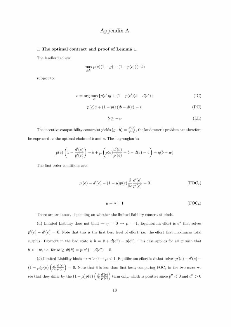
The landlord solves:

maxg,b

p(e)(1− g) + (1− p(e))(−b)

subject to:

e = argmaxe0{p(e0)g + (1− p(e0))b− d(e0)} (IC)

p(e)g + (1− p(e))b− d(e) = v (PC)

b ≥ −w (LL)

The incentive compatibility constraint yields (g−b) = d0(e)p0(e) , the landowner’s problem can therefore

be expressed as the optimal choice of b and e. The Lagrangian is:

p(e)

µ1− d

0(e)p0(e)

¶− b+ µ

µp(e)

d0(e)p0(e)

+ b− d(e)− v¶+ η(b+w)

The first order conditions are:

p0(e)− d0(e)− (1− µ)p(e) ∂∂e

d0(e)p0(e)

= 0 (FOCe)

µ+ η = 1 (FOCb)

There are two cases, depending on whether the limited liability constraint binds.

(a) Limited Liability does not bind → η = 0 → µ = 1. Equilibrium effort is e∗ that solves

p0(e) − d0(e) = 0. Note that this is the first best level of effort, i.e. the effort that maximizes total

surplus. Payment in the bad state is b = v + d(e∗) − p(e∗). This case applies for all w such that

b > −w, i.e. for w ≥ w(v) = p(e∗)− d(e∗)− v.(b) Limited Liability binds→ η > 0→ µ < 1. Equilibrium effort is e that solves p0(e)− d0(e)−

(1 − µ)p(e)³

∂∂ed0(e)p0(e)

´= 0. Note that e is less than first best; comparing FOCe in the two cases we

see that they differ by the (1−µ)p(e)³

∂∂ed0(e)p0(e)

´term only, which is positive since p00 < 0 and d00 > 0

18

and hence ∂∂ed0(e)p0(e) =

d00p0−d0p00(p0)2 > 0 for any e. Using the fact that p00 < 0 and d00 > 0 (i.e. surplus

is a concave function of e) we see that e must be smaller than e∗ to satisfy the first order condition.

Payment in the bad state is b = −w. This case applies for w < w(v).

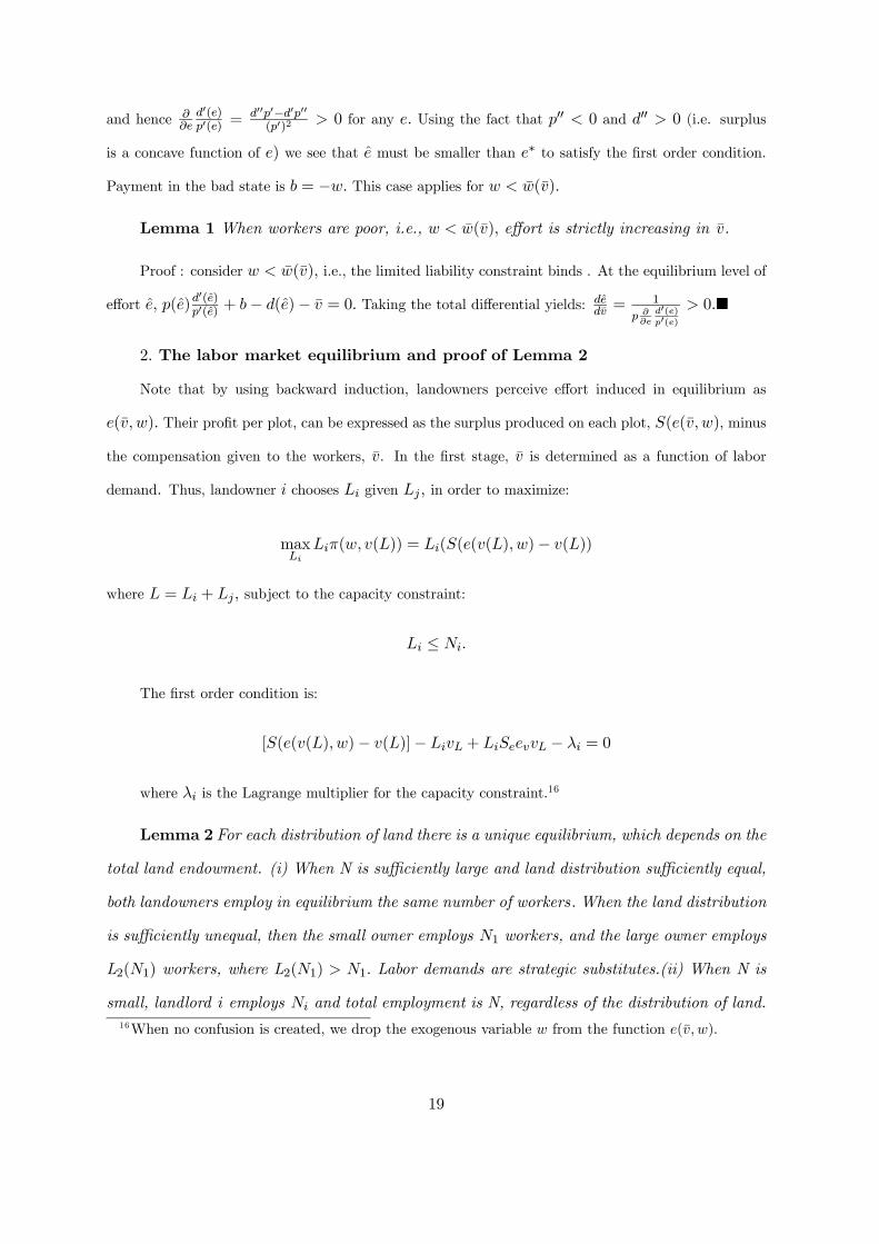
Lemma 1 When workers are poor, i.e., w < w(v), effort is strictly increasing in v.

Proof : consider w < w(v), i.e., the limited liability constraint binds . At the equilibrium level of

effort e, p(e)d0(e)p0(e) + b− d(e)− v = 0. Taking the total differential yields: dedv = 1

p ∂∂e

d0(e)p0(e)

> 0.¥

2. The labor market equilibrium and proof of Lemma 2

Note that by using backward induction, landowners perceive effort induced in equilibrium as

e(v, w). Their profit per plot, can be expressed as the surplus produced on each plot, S(e(v, w), minus

the compensation given to the workers, v. In the first stage, v is determined as a function of labor

demand. Thus, landowner i chooses Li given Lj , in order to maximize:

maxLiLiπ(w, v(L)) = Li(S(e(v(L), w)− v(L))

where L = Li + Lj , subject to the capacity constraint:

Li ≤ Ni.

The first order condition is:

[S(e(v(L), w)− v(L)]− LivL + LiSeevvL − λi = 0

where λi is the Lagrange multiplier for the capacity constraint.16

Lemma 2 For each distribution of land there is a unique equilibrium, which depends on the

total land endowment. (i) When N is sufficiently large and land distribution sufficiently equal,

both landowners employ in equilibrium the same number of workers.When the land distribution

is sufficiently unequal, then the small owner employs N1 workers, and the large owner employs

L2(N1) workers, where L2(N1) > N1. Labor demands are strategic substitutes.(ii) When N is

small, landlord i employs Ni and total employment is N, regardless of the distribution of land.16When no confusion is created, we drop the exogenous variable w from the function e(v, w).

19

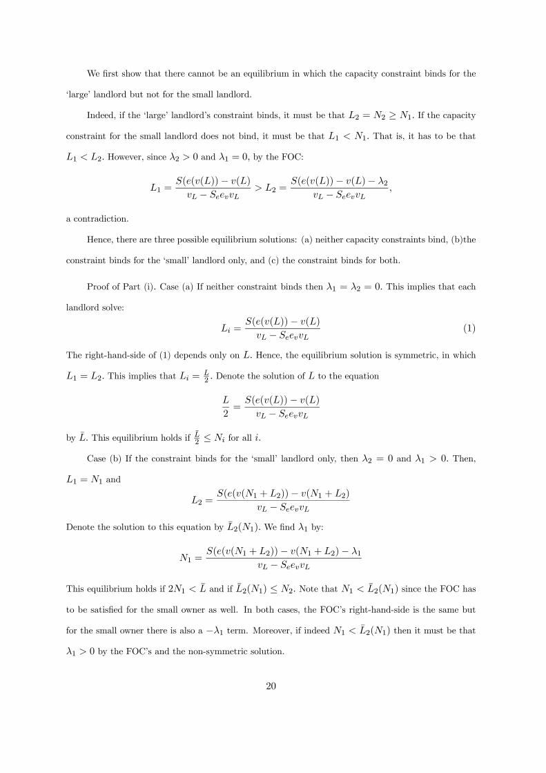
We first show that there cannot be an equilibrium in which the capacity constraint binds for the

‘large’ landlord but not for the small landlord.

Indeed, if the ‘large’ landlord’s constraint binds, it must be that L2 = N2 ≥ N1. If the capacityconstraint for the small landlord does not bind, it must be that L1 < N1. That is, it has to be that

L1 < L2. However, since λ2 > 0 and λ1 = 0, by the FOC:

L1 =S(e(v(L))− v(L)vL − SeevvL > L2 =

S(e(v(L))− v(L)− λ2vL − SeevvL ,

a contradiction.

Hence, there are three possible equilibrium solutions: (a) neither capacity constraints bind, (b)the

constraint binds for the ‘small’ landlord only, and (c) the constraint binds for both.

Proof of Part (i). Case (a) If neither constraint binds then λ1 = λ2 = 0. This implies that each

landlord solve:

Li =S(e(v(L))− v(L)vL − SeevvL (1)

The right-hand-side of (1) depends only on L. Hence, the equilibrium solution is symmetric, in which

L1 = L2. This implies that Li =L2 . Denote the solution of L to the equation

L

2=S(e(v(L))− v(L)vL − SeevvL

by L. This equilibrium holds if L2 ≤ Ni for all i.Case (b) If the constraint binds for the ‘small’ landlord only, then λ2 = 0 and λ1 > 0. Then,

L1 = N1 and

L2 =S(e(v(N1 + L2))− v(N1 + L2)

vL − SeevvLDenote the solution to this equation by L2(N1). We find λ1 by:

N1 =S(e(v(N1 + L2))− v(N1 + L2)− λ1

vL − SeevvL

This equilibrium holds if 2N1 < L and if L2(N1) ≤ N2. Note that N1 < L2(N1) since the FOC hasto be satisfied for the small owner as well. In both cases, the FOC’s right-hand-side is the same but

for the small owner there is also a −λ1 term. Moreover, if indeed N1 < L2(N1) then it must be thatλ1 > 0 by the FOC’s and the non-symmetric solution.

20

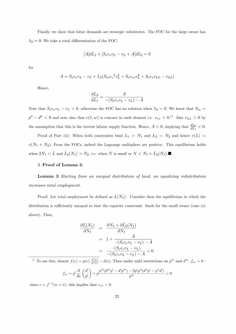
Finally, we show that labor demands are strategic substitutes. The FOC for the large owner has

λ2 = 0. We take a total differentiation of the FOC:

[A]dL1 + [SeevvL − vL +A]dL2 = 0

for

A = SeevvL − vL + L2(Seeev2v2L + Seevvv2L + SeevvLL − vLL)

Hence,

dL2dL1

=A

−(SeevvL − vL)−ANote that SeevvL − vL < 0, otherwise the FOC has no solution when λ2 = 0. We know that See =p00 − d00 < 0 and note also that e(v, w) is concave in each element i.e. evv < 0.17 Also vLL > 0 bythe assumption that this is the inverse labour supply function. Hence, A < 0, implying that dL2dL1

< 0.

Proof of Part (ii): When both constraints bind L1 = N1 and L2 = N2 and hence v(L) =

v(N1 + N2). From the FOCs, indeed the Lagrange multipliers are positive. This equilibrium holds

when 2N1 < L and L2(N1) > N2, i.e. when N is small or N < N1 + L2(N1).¥

3. Proof of Lemma 3.

Lemma 3 Starting from an unequal distribution of land, an equalizing redistribution

increases total employment.

Proof: Let total employment be defined as L(N1). Consider then the equilibrium in which the

distribution is sufficiently unequal so that the capacity constraint binds for the small owner (case (a)

above). Then,

∂L(N1)

∂N1=

∂N1 + ∂L2(N1)

∂N1

= 1 +A

−(SeevvL − vL)−A=

−(SeevvL − vL)−(SeevvL − vL)−A > 0.

17 To see this, denote f(e) = p(e) d0(e)p0(e) − d(e). Then under mild restrictions on p000 and d000, fee > 0 :

fee = p0 ∂∂e

µd0

p0

¶+ p

p02(d000p0 − d0p000)− 2p0p00(d00p0 − p00d0)p04

> 0

since e = f−1(w + v), this implies that evv < 0.

21

When the distribution is equal enough so that neither capacity constraint bind and as long as

redistribution does not alter the ranking, i.e. the small owner always owns at most the same number

of plots as the large owner, we get the same symmetric solution and hence ∂L(N1)∂N1

= 0. ¥

4. Proof of Proposition 1.

Proposition 1 Starting from a sufficiently unequal distribution of land, an equalizing

redistribution among landowners results into higher employment and, when workers are poor,

higher effort. Total surplus increases as a consequence and reaches its maximum when the

distribution of land becomes sufficiently equal.

Proof: Total surplus is equal to:

TS(N1) = L(N1) · S(N1) = L(N1)S(e(v(L(N1)))

Taking the derivative w.r.t. N1 :

∂TS(N1)

∂N1=

∂L

∂N1S +

∂S

∂N1L

=∂L

∂N1S + SeevvL

∂L

∂N1L

=∂L

∂N1(S + SeevvLL) > 0.

From Lemma 3 we know that ∂L∂N1

> 0 when the initial distribution is unequal (i.e. the capacity

constraint binds for the small owner) and from Lemma 1 we know that ev > 0 when the limited liability

constraint binds. Hence when workers are poor and the initial distribution is unequal, redistribution

increases both employment and effort. When workers are relatively rich and the initial distribution

is unequal, redistribution increases employment and maintains the same effort level. When the initial

distribution is sufficiently equal (i.e. when neither capacity constraint binds), Lemma 3 shows that

∂L∂N1

= 0 and hence total surplus is unchanged.¥

5. Proof of Proposition 2.

Proposition 2 Starting from a sufficiently unequal distribution of land, an equalizing

redistribution among landowners leads to:

(i) an increase in the welfare of each inframarginal worker;

22

(ii) an increase in the profits of the small landowner;

(iii) a decrease in the profits of the large landowner and of the joint profits of both landown-

ers.

Proof: (i) When N1 increases all the inframarginal workers earn more net of disutility costs and

hence their welfare increases.

(ii) Recall that the first order condition for the large landlord is:

S(e(v(L(N1)))− v(L(N1)) + L2(SeevvL − vL) = 0

The welfare of the small landlord is equal to N1(S(e(v(L(N1)))− v(L(N1))), therefore:

∂N1(S(e(v(L(N1)))− v(L(N1)))∂N1

= S(e(v(L(N1)))− v(L(N1)) +N1∂L(N1)∂N1

(SeevvL − vL)

= S(e(v(L(N1)))− v(L(N1))(1− N1L2

∂L(N1)

∂N1)

but S − v > 0 for any level of employment, N1L2 < 1, and

∂L(N1)

∂N1=

∂(N1 + L2(N1))

∂N1= 1 +

∂L2(N1)

∂N1< 1.

because ∂L2(N1)∂N1

< 0. It follows that

∂N1(S(e(v(L(N1)))− v(L(N1)))∂N1

> 0

i.e., the welfare of the small landlord increases.

(iii) The joint welfare of landlords L(S(e(v(L))−v(L)) is obviously maximized when one of themis a monopolist, i.e. when N1 = 0. It then follows that, by curtailing monopoly power, redistribution

causes the joint welfare to fall. Since the joint welfare of the landlords decreases and the welfare of the

small landlord increases, the welfare of the large landlord must decrease.¥

Appendix B

Many landowners Consider z landlords, ordered by N1 < N2 < ... < Nz.Consider the maxi-

mization problem of landlord i :

23

maxLiLi(S(e(v(L)− v(L)) + λi(Ni − Li),

where L =Pzj=1 Lj . The FOC has:

Li =S(e(v(L))− v(L)− λi

vL − SeevvLwhere λi is the Lagrange multiplier of the capacity constraint for landowner i. It can be easily

verified that if the capacity constraint for landlord i binds, it must also bind for all landlord j < i.

Hence, equilibria are characterized by the number of binding constraints k, k ∈ {0, 1, ..., z}, whereLi = Ni for i ≤ k. For i > k, the equilibrium solution is symmetric by the FOC where λi = 0.

The existence of these equilibria depends on the distribution of land. In particular, with a com-

pletely equal distribution of assets, and high enough N, a symmetric equilibrium exists in which neither

capacity constraint binds, i.e., k = 0. The condition for this equilibrium to hold is L(NZ)z ≤ Ni for all

i, where L(NZ) is defined by the equation below:

L

z=S(e(v(L))− v(L)vL − SeevvL

Consider a transfer of land from a landowner whose constraint does not bind to the richest

landowner for whom the constraint binds. Assume first that the transfer is such that the capacity

constraint still binds for the landowners that receives the transfer. Then, the total differential of the

FOC for the landowner whose constraint does not bind yields:

A(k−1Xi=1

dNi + dNk +zX

h=k+1,h6=jdLh(N

Z)) + [SeevvL − vL +A]dLj(NZ) = 0 (2)

for

A = SeevvL − vL + Lj(Seeev2v2L + Seevvv2L + SeevvLL − vLL) < 0

Note however that dNi = 0 for all i < k, and that by symmetry, dLh(NZ) = dLj(NZ) for all

j, h > k. Then, re-arranging (2), we get:

AdNk + [SeevvL − vL + (k − b)A]dLj(NZ) = 0→dLj(N

Z)

dNk=

A

−[SeevvL − vL + (z − k)A] < 0

24

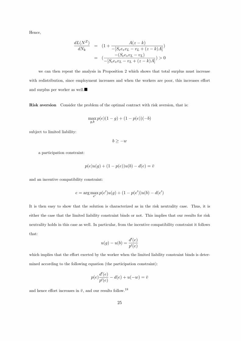
Hence,

dL(NZ)

dNk= (1 +

A(z − k)−[SeevvL − vL + (z − k)A] )

= (−(SeevvL − vL)

−[SeevvL − vL + (z − k)A] ) > 0

we can then repeat the analysis in Proposition 2 which shows that total surplus must increase

with redistribution, since employment increases and when the workers are poor, this increases effort

and surplus per worker as well.¥

Risk aversion Consider the problem of the optimal contract with risk aversion, that is:

maxg,b

p(e)(1− g) + (1− p(e))(−b)

subject to limited liability:

b ≥ −w

a participation constraint:

p(e)u(g) + (1− p(e))u(b)− d(e) = v

and an incentive compatibility constraint:

e = argmaxe0p(e0)u(g) + (1− p(e0))u(b)− d(e0)

It is then easy to show that the solution is characterized as in the risk neutrality case. Thus, it is

either the case that the limited liability constraint binds or not. This implies that our results for risk

neutrality holds in this case as well. In particular, from the incentive compatibility constraint it follows

that:

u(g)− u(b) = d0(e)p0(e)

which implies that the effort exerted by the worker when the limited liability constraint binds is deter-

mined according to the following equation (the participation constraint):

p(e)d0(e)p0(e)

− d(e) + u(−w) = v

and hence effort increases in v, and our results follow.18

25

References

[1] Baland, J.M. and J. Robinson (2003) “Land and Power” CEPR Discussion Paper 3800

[2] Bandiera, O. (2003), “Land Tenure, Incentives and the Choice of Techniques: Evidence from

Nicaragua.”, mimeo London School of Economics and STICERD.

[3] Banerjee, A.V., Gertler, P.J. and Ghatak, M. (2002), “Empowerment and Efficiency: Tenancy

Reform in West Bengal”, Journal of Political Economy, 110(2), 239-280.

[4] Banerjee, A.V. (1999), “Land Reforms: Prospects and Strategies”, Massachusetts Institute of

Technology, Department of Economics Working Paper: 99/24.

[5] Bell, C. (1990) “Reforming Property Rights in Land and Tenancy”, World Bank Research Ob-

server.

[6] Besley, T. and R. Burgess (2000) “Land Reform, Poverty Reduction, And Growth: Evidence From

India.” The Quarterly Journal of Economics,115(2), 389-430.

[7] Berry, R.A., and Cline, W.R. (1979), Agrarian structure and productivity in developing countries.

Geneva: International Labor Organization.

[8] Binswanger, H., Deininger, K., and Feder, G. (1995), “Power, Distortions, Revolt and Reform in

Agricultural Land Relations”, in: Behrman, J. and Srinivasan, T.N. (Eds.), Handbook of Devel-

opment Economics,III (Ch. 42): 2659-2772, Elsevier Science

[9] Dasgupta, P. and Ray, D. (1986) “Inequality as a Determinant of Malnutrition and Employment:

Theory”, Economic Journal, 96, 1011-34.

[10] Dasgupta, P. and Ray, D. (1987) “Inequality as a Determinant of Malnutrition and Employment:

Policy”, Economic Journal, 97, 177-88.

[11] Deininger, K. and Feder, G. (1998), Land Institutions and Land Markets, World Bank Work-

ing Paper no 2014 - Handbook of Agricultural Economics (B. Gardner and G. Rausser, Eds),

forthcoming.18Note that, however, if the workers are risk averse first best cannot be achieved even if the limited liability

constraint does not bind.

26

[12] Dutta, B., Ray,D. and Sengupta, K. (1989), “Contracts with Eviction in Infinitely Repeated

Principal-Agent Relationships”, Bardhan, P. ed. Oxford; New York; Toronto and Melbourne: The

economic theory of agrarian institutions. Oxford University Press 1989; 93-121

[13] Moene, K. (1992), “Poverty and Landownership” The American Economic Review, 82 (1), 52-64.

[14] Mookherjee, D. (1997), “Informational Rents and Property Rights in Land,” in J. Roemer, ed.,

Property Rights, Incentives and Welfare, New York: MacMillan Press.

[15] Mookherjee D. and Ray D (2002), “Contractual Structure and Wealth Accumulation”, American

Economic Review 92(4), 818-849.

[16] Rosenzweig, M. and Binswanger, H. (1993), “Wealth, Weather Risk and the Composition and

Profitability of Agricultural Investments”, Economic Journal 103(416), pages 56-78.

[17] Shaban,R.A. (1987), “Testing Between Competing Models of Sharecropping”, Journal of Political

Economy 95(5), 893-920.

[18] Shapiro, C. and J. E. Stiglitz (1984) “Equilibrium Unemployment as a Worker Discipline Device”

American Economic Review 74(3), 433-44

27