Robert G. King and Sergio T. Rebelo Rochester Center for ...

Low Frequency Filtering and Real Business Cycles

Robert G. King and Sergio T. Rebelo

Rochester Center for Economic Research Working Paper No. 205

LOW FREQUENCY FILTERING AND REAL BUSINESS CYCLES

Robert G. King University of Rochester

and Rochester Center for Economic Research

AND Sergio T. Rebelo

Northwestern University Portuguese Catholic University

and Rochester Center for Economic Research

Working Paper No. 205

February 1988 Revised: October 1989

The authors acknowledge financial support from the National Science Foundation. This research has benefited from discussions with Marianne Baxter, Gary Hansen, Robert Hodrick, Charles Plosser, Edward Prescott and Mark Watson. However, the authors are residual claimants with respect to errors of any sort.

Lo. Frequency Filtering and Real Business Cycles

Abstract

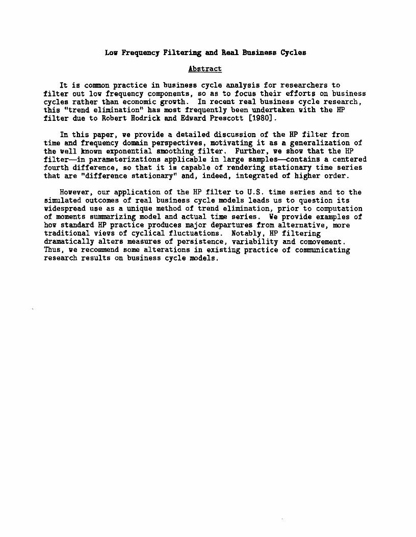
It is common practice in business cycle analysis for researchers to filter out lov frequency components, so as to focus their efforts on business cycles rather than economic grovth. In recent real business cycle research, this IItrend eliminationll has most frequently been undertaken vith the HP filter due to Robert Hodrick and Edvard Prescott [1980].

In this paper, ve provide a detailed discussion of the HP filter from time and frequency domain perspectives, motivating it as a generalization of the veIl know exponential smoothing filter. Further, ve shov that the HP filter--in parameterizations applicable in large samples--contains a centered fourth difference, so that it is capable of rendering stationary time series that are "difference stationary" and, indeed, integrated of higher order.

Hovever, our application of the HP filter to U.S. time series and to the simulated outcomes of real business cycle models leads us to question its vide spread use as a unique method of trend elimination, prior to computation of moments summarizing model and actual time series. We provide examples of hov standard HP practice produces major departures from alternative, more traditional vievsof cyclical fluctuations. Rotably , HP filtering dramatically alters measures of persistence, variability and comovement. Thus, ve recommend some alterations in existing practice of communicating research results on business cycle models.

I. Introduction

1 hallmark of modern equilibrium business cycle theory is the viev that

grovth, business cycles and seasonal variations are to be studied vithin a

unified framevork. Even though rational economic agents are presumed to

respond differently to shocks of varying duration, dynamic economic theory

generally imposes concrete and extensive restrictions across frequencies.

For one example, the manner in vhich agents respond to varying seasonal

opportunities provides information about hov they viII respond to temporary

opportunities during the course of business cycles. For another, the manner

in vhich labor supply responds to the permanent vage and vealth changes

occurring during economic grovth restricts responses at business cycle

frequencies.

Yet, beginning vith Kydland and Prescott [1982], many studies in the real

business cycle research area apply the HP filter--due to Hodrick and Prescott

[1980]--to both time series generated from an artificial economy and actual

data before making conclusions about the properties of the model and its

congruence vith observations. This practice corresponds to an implicit

definition of "the business cycle frequencies" and a decision to domplay the

implications of the model at other frequencies, generally on the grounds that

these represent grovth rather than business cycles.

Reading the literature on real business cycles, one can easily come to

the conclusion that the practice of "lov frequency filtering" has relatively

minor consequences for hov one thinks about economic models and their

consistency vith observed time series. This paper demonstrates that the

opposite conclusion is true: the practice of lov frequency filtering has

major consequences for both the "stylized" facts of business cycles and the

perceived operation of dynamic economic models. In fact, the components of

2

time series removed by mechanical application of the HP filter are

sufficiently important that one may feel that the baby is being thro~n out

vith the bath vater in terms of business cycle research. Consequently, ~e

provide some specific recommendations for alterations in practice, i.e., in

the reporting of research results on business cycles.

Our motivation for this investigation derived from tvo sources, ~hich ~e

provide to the reader as a puzzle to be investigated in the remainder of the

paper.

Implications for Simulated Time Series

Our first exposure to the potential importance of HP filtering involved

an attempt to replicate some results obtained in Gary Hansen's [1985] analysis

of the effects of varying the labor supply elasticity in a basic real

business cycle model. 1

Table 1-1 provides a fe~ population moments, basically those reported by

Hansen [1985], vith and vithout HP filtering.2 The model economy is one in

vhich the single source of uncertainty is a trend stationary technology shock

to total factor productivity; it is detailed in King, Plosser and Rebelo

[1988a] and revieved in section III belovo From this table, it is clear that

HP filtering alters the moment implications of the model in a quantitatively

important manner, but that this influence is not constant across series.

lWe thank Gary Hansen for providing some simulation results for unfiltered versions of his model [1985] that confirmed our conjectures that filtering, not model solution methods or model parameter values, lay at the heart of major differences in moments. 2Reporting of these selected moments is common in discussions of implications of real business cycle models, as-for example--in McCallum's [1989] survey, Tables 1 and 2. .

3

First, HP filtering, vhich extracts a component from the original series,

lovers volatility as measured by the standard deviation columns in table 1.

Second, HP filtering alters the relative volatilities of different series

(the standard deviation of a variable divided by that of output). In

particular. it increases the relative volatility of investment and hours

vhile lovering that of consumption. the real vage and the capital stock.

Third, the correlations betveen individual series and output--a measure of

cyclical sensitivity--are substantially altered by HP filtering. Notably,

the cyclical variation in capital and labor input is dramatically altered by

filtering. In the unfiltered economy, capital's correlation with output is

.73 and that of labor vith output is .79. With filtering. capital's

correlation drops to .07 and that of labor rises to .98.

HP Filtering of Some U.S. Post War Time Series

Our second indication of the potential importance of HP filtering came

from Marianne Baxter's empirical vork (Baxter [1988] and Baxter and Stockman

[1988]) on stylized facts of economic fluctuations in the United States and

other countries. 3 To provide some empirical background to our subsequent

analysis. ve begin by displaying an application of the HP filter to a measure

of aggregate economic activity and a measure of labor input. These are the

logarithm of U.S. real gross national product, which ve denote Yt' and the

logarithm of per capita average hours vorked, vhich ve denote Nt'

3We thank Marianne Baxter for suggesting the revealing examples contained in this section and for technical assistance in producing these results.

4

Like other lov frequency filters, the BP filter can be vieved as

extracting grovth and cyclical components from the data. 4 To start, let us

focus on the Yt series and begin by dividing Yt into a linear trend (7t) and

a residual deviation from a linear trend (so that the residual y~ = Yt - 7t).

If the grovth component is assumed to be a deterministic trend, then the

business cycle component is y~. Under the BP filtering procedure, by

contrast, the time series is permitted to have a stochastic grovth component.

In addition to extracting a linear trend--if one exists in the series under

study--HP filtering also removes some additional variation vhose properties

depend on the series in vays detailed in section II belov. The HP cyclical

component is then defined as the difference betveen the original time series

and the HP grovth component.

Implications for Real GNP: Figure 1-1 plots the HP grovth component versus

the linear trend component of real gross national product. A relatively

common reaction to this figure is that these vays of removing grovth are not

too different. But it turns out that there are major consequences for

business cycle components.

In order to study the practical implications of alternative detrending

methods J ve construct the HP stochastic grovth component by subtracting a

linear trend from the BP grovth component (taking the vertical difference

betveen the series in Figure 1). Ve call this component HPg(Yt)'

4In part, our discussion in this section and belov involves the issue of how best to define business cycles. One possibility--vhich is sometimes discussed in evaluation of mechanical procedures such as the HP filter--vould be to select some mechanical method that broadly replicated the stylized facts reported by IBER researchers folloving Mitchell [1927,1961] and Burns and Mitchell [1941]. Hovever, preliminary vork by King and Plosser [1989] leads us to believe that the RBER methods should be subject to some scrutiny as veIl.

5

Summarizing our definitions, the alternative decompositions are

Yt = 1t + y~ = 1t + HPcCYt) + HPgCyt ),

i.e., the HP cyclical and stochastic grovth components sum to the residual

from the deterministic trend.

Figure 1-2 makes clear that the HP stochastic grovth component

constitutes a major portion of the departure of output from a linear trend,

so that the implied cyclical components arising from these tvo methods of

trend elimination are very different both in terms of magnitude and

persistence. Notably, the autocorrelation correlation coefficient of y~ at

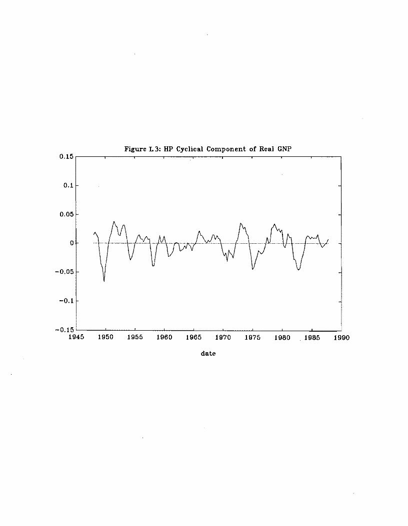
the annual lag is .72. Figure 1-3 plots the HP cyclical component CHpc(Yt»

of real GIP, vhich is a rapidly fluctuating series, as may be judged from its

autocorrelation structure, vhich is' presented in Table 1-2, panel A. The

autocorrelation at a year lag (four quarters), for example, is only .09,

vhich is an order of magnitude smaller than the autocorrelation coefficient

for HprCYt) at the same lag.

Implications for GNP and Labor Input: Figure 1-4 plots y~ versus the

departures of our labor input measure from its mean (i.e., It-I). There is

not a strong relationship: the contemporaneous correlation is only .06.

Hovever, vhen one compares the HP cyclical components of output and hours in

Figure 1-5, there is a striking coincidence: the contemporaneous correlation

is .86. Further information on the implications of filtering for

correlations among variables is contained in Table 1-2.

Outline of Our Analysis

To this point, ve have shovn that lov frequency filtering--using the

Hodrick and Prescott [1980] filter--has important implications on moments of

6

U.S. time series and a simulated real business cycle model. In developing an

explanation of the origin of these results and their practical consequences

for business cycle research ve proceed as follovs. In section II, ve first

discuss vhat linear filtering is and then reviev some facts about linear

filters. We next derive the HP growth and cyclical filters as a direct

generalization of the well-known exponential smoothing filter of Brown

[1962]. In section III, we apply the HP filter to some basic real business

cycle models to further develop the sorts of implications suggested by

section III. Building on these results, in section IV, we provide a

concrete set of recommendations about how to best report results of

investigations into business cycles. Section V is a brief summary and

conclusion.

II. to.. Frequency Filtering

There is a lengthy history in macroeconomics of filtering time series.

For example, there is extensive use of moving averages of time series by

Mitchell [1930] and Kuznets [1930] in their analyses of business cycles and

economic growth. Further, applications of moving averages and other linear

filters can sometimes lead to important statistical artifacts in time series.

For example, Fishman [1969] summarizes research that points out how the

apparent long swings in economic activity suggested by Kuznets [1961] might

potentially have arisen simply from his application of moving averages rather

than as a property of underlying economic time series.

In this section, our objectives are twofold. First, in section 11.1, ve

provide an overview of analytical tools for studying the implications of

linear filters. This section should be skipped by readers who are

comfortable with introductory treatments of frequency domain methods (e.g.,

7

Harvey [1981, Chapter 3]). Second, in section 11.1, we motivate the HP

filter as a generalization of the familiar class of exponential smoothing

(ES) procedures studied by Brown [1962]. Throughout our discussion in this

section, we will focus our attention on a representative time series Yt'

which we treat as the logarithm of an original series so that its first

difference is a growth rate.

In filtering Yt' a researcher is motivated by one of several objectives:

(i) extraction of a component such as a growth, cyclical or seasonal

component; (ii) transformation to induce stationarity; or (iii) mitigation of

measurement error that is assumed to be particularly important at specific

frequencies. We concentrate on the first two motivations, since a detailed

treatment of measurement error would require grappling with details of a

specific application.

To focus our discussion, then, consider the idea that a particular

economic model makes predictions about a IIbusiness cycle" component of a time

series and that the researcher views the series as containing both growth and

business cycle components.

where yf is the growth component and y~ is the business cycle component.

Representing yf as a moving average (possibly two sided) of observed Yt

permits extraction of the growth component (Y~) and the cyclical component

(Y~)' That is. suppose that we assume that

(I)

yf. E g. Yt . - G(B) Yt'j--m J -J

where B is the backshift operator with snx = x _ for n ~ O. Then, sincet t n

- -

8

cit fo110vs that Yt is also a moving average of Yt'

y~ • [1 - G(B)] Yt == C(B) Yt'

In the language of filtering theory. G(B) and C(B) = [1 - G(B)] are linear

filters and ve nov explore some of their properties.

11.1 So.. Facts ~bout Linear Filters

In order to discuss vhy a specific linear filter may be described as a low

frequency filter, ve are led to consideration of the Fourier transform ofa

linear filter (also called the frequency response function of the filter).

For example. the frequency response of the grovth filter is .

_ !II

G(w) = E g. exp (-ijw) j=-m J

vhere i denotes the imaginary number Jr=ff and vhere w is frequency measured

in radians. i.e., -11' S w S 71".

Gain and Phase Decomposition: At a given frequency w, the frequency -

response G(w) is simply a complex number, so that it may be vritten in polar

form as G(w)=r(w)exp(-i~(w», vhere r(w)=IG(w) I and ~(w) are real numbers

for fixed w. In these expressions and belov, Ixl denotes the modulus of x

(the square root of the product of x and its conjugate). The gain of the

linear filter. r(w). yields a measure--at the specified frequency ~f the

increase in the amplitude of the filtered series over the original series.

The phase, ~(w). yields a measure of the time displacement attributable to

the linear filter, again at the specified frequency w. The frequency

response function can be decomposed into the gain function r(w) and phase

function ~(w) by replicating the preceding decomposition at each value of w.

9

To take a concrete example, suppose that a time series is strictly

periodic vith a period of 2~/w*. Then application of the linear filter G

vould simply alter the range of this periodic function by r(w*)=IG(w*) I. as

illustrated in Figure II-la. Further, Figure II-lb illustrates the

hypothetical phase shift effect of a linear filter,

Symmetric Filters: In our analysis, ve viII focus on filters that possess a

symmetry property in that gj = g_j' For any such filter, it is possible to

shov that

_ III

G(w) =go + 2 E gj cos (jw)j=l

using the trigonometric identity 2cos(x) = {exp(ix) + exp(-ix)}. Symmetric

filters have the important property that they do not induce a phase shift. -

i.e., W(w) = 0 for all w, since the Fourier transform G(w) is real for a

symmetric filter, Thus, the gain function is equal to the frequency

response, so that ve use these terms interchangeably belovo

Further, in the class of symmetric filters. it is easy to see that

III-G(O) = E g. = 1

j--oo J

is a necessary and sufficient condition for a filter to have the property

that it has unit gain at zero frequency,S Thus, by extension, the associated

cyclical filter C(B) = [1 - G(B)] viII place zero veight on zero frequency -

vhenever G(O) • 1.

wrhis property obtains for symmetric filters since cos(O)=l and it follows-directly that G(O) -1. Moreover, this property holds as well for-nonsymmetric filters since exp(O) =1 implies that G(O)=lunder the condition that the filter veights sum to unity.

10

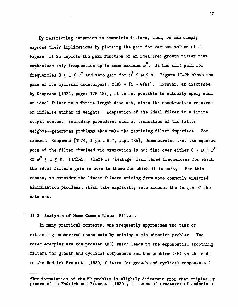
By restricting attention to symmetric filters, then, ve can simply

express their implications by plotting the gain for various values of w.

Figure II-2a depicts the gain function of an idealized grovth filter that

emphasizes only frequencies up to some maximum w·. It has unit gain for

frequencies 0 ~ w ~ w· and zero gain for w· ~ w ~~. Figure II-2b shovs the

gain of its cyclical counterpart, C(B) • [1 - G(B)]. Hovever, as discussed

by Koopmans [1974, pages 176-186], it is not possible to actually apply such

an ideal filter to a finite length data set, since its construction requires

an infinite number of veights. Adaptation of the ideal filter to a finite

veight context--including procedures such as truncation of the filter

veights--generates problems that make the resulting filter imperfect. For

example, Koopmans [1974, figure 6.7, page 186], demonstrates that the squared

gain of the filter obtained via truncation is 'not flat over either 0 ~ w ~ w*

or w• ~ w ~~. Rather, there is "leakage" from those frequencies for vhich

the ideal filter's gain is zero to those for vhich it is unity. For this

reason, ve consider the linear filters arising from some commonly analyzed

minimization problems, vhich take explicitly into account the length of the

data set.

11.2 Analysis of Some Common Linear Filters

In many practical contexts, one frequently approaches the task of

extracting unobserved components by solving a minimization problem. Tvo

noted examples are the problem (ES) vhich leads to the exponential smoothing

filters for grovth and cyclical components and the problem (HP) vhich leads

to the Hodrick-Prescott [1980] filters for grovth and cyclical components. 6

GOur formulation of the HP problem is slightly different from that originally presented in Hodrick and Prescott [1980], in terms of treatment of endpoints.

11

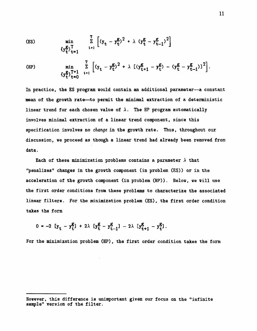
(ES)

(HP)

In practice, the ES program vould contain an additional parameter--a constant

mean of the grovth rate--to permit the minimal extraction of a deterministic

linear trend for each chosen value of A. The HP program automatically

involves minimal extraction of a linear trend component, since this

specification involves no change in the grovth rate. Thus, throughout our

discussion~ ve proceed as though a linear trend had already been removed from

data.

Each of these minimization problems contains a parameter A that

"penalizes" changes in the grovth component (in problem (ES» or in the

acceleration of the grovth component (in problem (HP». Belov, ve viII use

the first order conditions from these problems to characterize the associated

linear filters. For the minimization problem (ES), the first order condition

takes the form

o =-2 [y _.Jt] + 2A [yg - yg ] - 2A [_.Jt _ yg]t Yt t t-l Yt+l t'

For the minimization problem (HP), the first order condition takes the form

Hovever, this difference is unimportant given our focus on the "infinite sample" version of the filter.

12

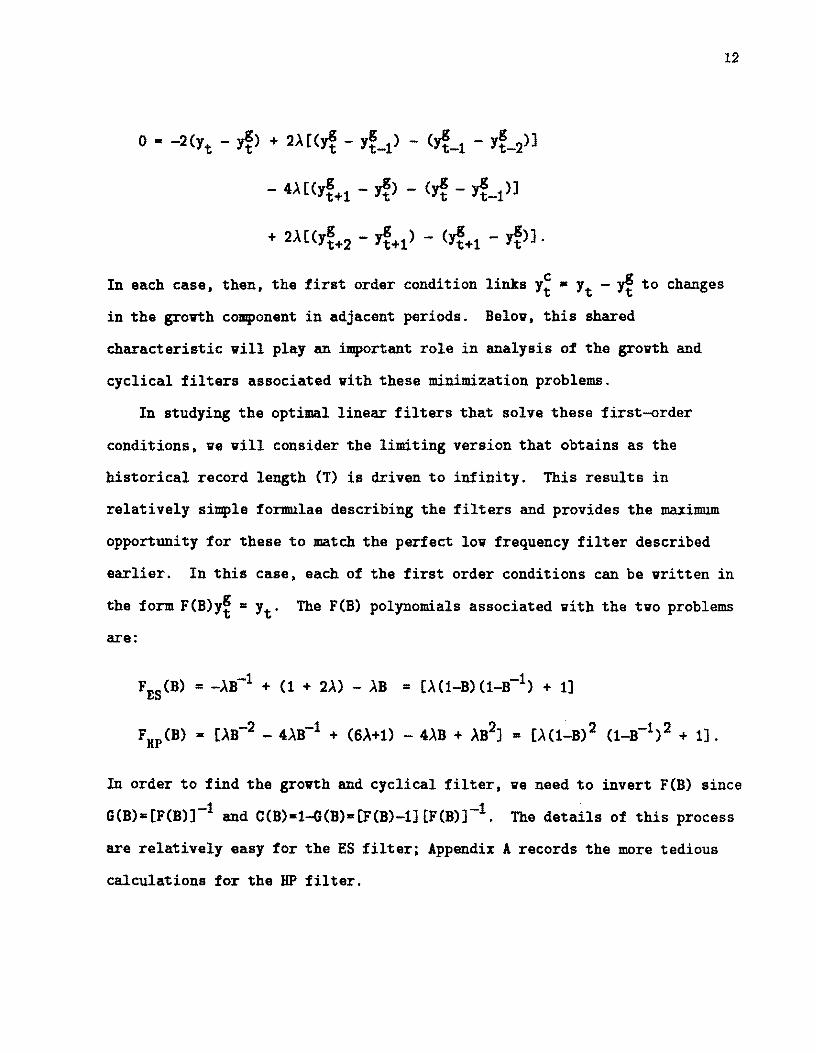
o =-2(Yt - yf) + 2A[(yf - yf-1) - (yf-1 - yf-2)]

- 4A[(yf+l - yf) - (yf - yf-1)]

In each case, then, the first order condition links y~ • Yt - yf to changes

in the growth component in adjacent periods. Belov, this shared

characteristic viII play an important role in analysis of the grovth and

cyclical filters associated vith these minimization problems.

In studying the optimal linear filters that solve these first-order

conditions, ve viII consider the limiting version that obtains as the

historical record length (T) is driven to infinity. This results in

relatively simple formulae describing the filters and provides the maximum

opportunity for these to match the perfect lov frequency filter described

earlier. In this case, each of the first order conditions can be vritten in

the form F(B)yf = Yt' The F(B) polynomials associated vith the tvo problems

are:

F (B) =_AB-1 + (1 + 2A) - AB = [A(1-B)(1-B-1) + 1]ES

In order to find the grovth and cyclical filter, ve need to invert F(B) since

G(B)=[F(B)]-1 and C(B)=1-G(B)=[F(B)-1] [F(B)]-1. The details of this process

are relatively easy for the ES filter; Appendix A records the more tedious

calculations for the UP filter.

13

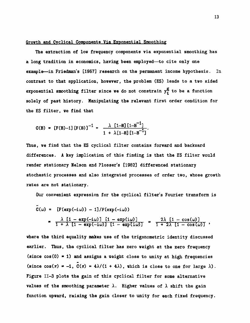
Growth and Cyclical Components Via Exponential Smoothing

The extraction of low frequency components via exponential smoothing has

a long tradition in economics, having been employed--to cite only one

example--in Friedman's [1967] research on the permanent income hypothesis. In

contrast to that application, hovever, the problem (ES) leads to a two sided

exponential smoothing filter since ve do not constrain yf to' be a function

solely of past history. Manipulating the relevant first order condition for

the ES filter, we find that

Thus, we find that the ES cyclical filter contains forward and backward

differences. A key implication of this finding is that the ES filter vould

render stationary Nelson and Plosser's [1982] differenced stationary

stochastic processes and also integrated processes of order tvo, whose growth

rates are not stationary.

Our convenient expression for the cyclical filter's Fourier transform is

-C(w) = [F(exp(-iw» - 1]/F(exp(-iw»

= A [1 - exp(-iw)] [1 - exp(iw)] 2A [1 - cos(w)]1 + X [1 - exp(-iw)] [1 - exp(iw)] = 1 + 2X [1 - cos(w)] ,

where the third equality makes use of the trigonometric identity discussed

earlier. Thus, the cyclical filter has zero weight at the zero frequency

(since cos(O) =1) and assigns a veight close to unity at high frequencies

-(since cos(~) =-1, C(~) =4A/(1 + 4A), which is close to one for large A).

Figure 11-3 plots the gain of this cyclical filter for some alternative

values of the smoothing parameter A. Higher values of A shift the gain

function upward, raising the gain closer to unity for each fixed frequency.

14

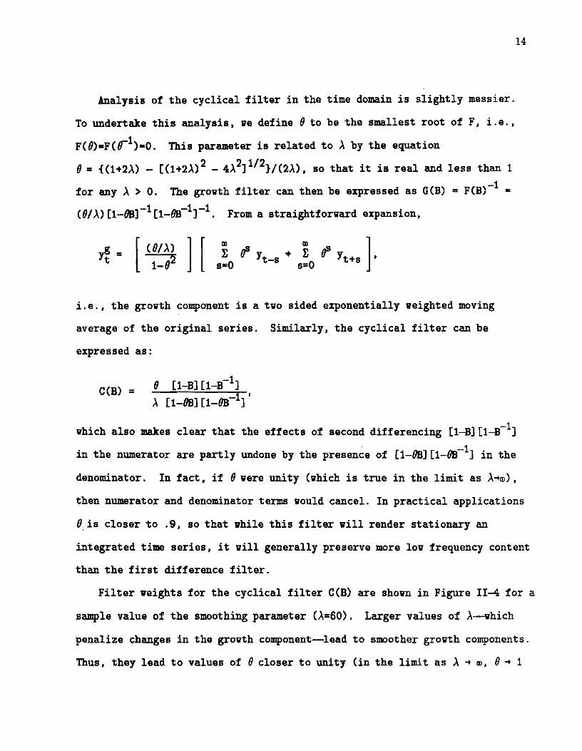
Analysis of the cyclical filter in the time domain is slightly messier.

To undertake this analysis, ve define 0 to be the smallest root of F, i.e.,

F(O)=F(,-l)=O. This parameter is related to A by the equation

0= {(1+2A) - [(1+2A)2 - 4A2]1/2}/(2A), so that it is real and less than 1

for any A > O. The grovth filter can then be expressed as G(B) = F(B)-l =

(O/A) [1_68]-1[1_68-1]-1. From a straightforvard expansion,

(O/A) ] [ E OS y + E OS y ],[ 1 02 0 t-s -0 t+s- s= s­

i.e., the grovth component is a tvo sided exponentially veighted moving

average of the original series. Similarly, the cyclical filter can be

expressed as:

o [i-B] [i-B-1]C(B) = A [1-68][1-OB-1]'

vhich also makes clear that the effects of second differencing [l-B] [1_B-1]

in the numerator are partly undone by the presen~e of [1-68] [1_eo-1] in the

denominator. In fact, if 0 vere unity (vhich is true in the limit as A~ro),

then numerator and denominator terms vould cancel. In practical applications

O,is closer to .9, so that vhile this filter viII render stationary an

integrated time series, it viII generally preserve more lov frequency content

than the first difference filter.

Filter veights for the cyclical filter C(B) are shown in Figure 11-4 for a

sample value of the smoothing parameter (A=GO). Larger values of A--vhich

penalize changes in the grovth component--Iead to smoother grovth components.

Thus, they lead to values of 0 closer to unity (in the limit as A ~ w, 0 ~ 1

15

so that C(B) • 1, i.e., Y~ • Yt ). The values of °for some alternative values

of A are given in Table 11-1.

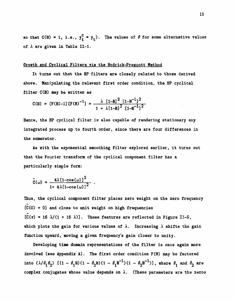
Grovth and Cyclical Filters via the Hodrick-Prescott Method

It turns out that the HP filters are closely related to those derived

above. Manipulating the relevant first order condition, the HP cyclical

filter C(B) may be vritten as

1C(B) = [F(B)-l] [F(B)-l] = A [1_B]2 [1_B- ]2

1 + A[1-B]2 [1_B-1]2

Hence, the HP cyclical filter is also capable of rendering stationary any

integrated process up to fourth order, since there are four differences in

the numerator.

As vith the exponential smoothing filter explored earlier. it turns out

that the Fourier transform of the cyclical component filter has a

particularly simple form:

- 4A[1-cos(w)]2C(w) = 1+ 4A[1-cos(w)]2

Thus, the cyclical component filter places zero veight on the zero frequency

-[C(O) = 0] and close to unit veight on high frequencies -[C(~) = 16 A/(l + 16 A)]. These features are reflected in Figure 11-5.

vhich plots the gain for various values of A. Increasing A shifts the gain

function upvard. moving a given frequency's gain closer to unity.

Developing time domain representations of the filter is once again more

involved (see Appendix A). The first order condition F(B) may be factored

into (AI0102) [(1 - 0lB) (1 - 02B) (1 - 0lB-1)(1 - °2B- 1)], vhere 01 and 02 are

complex conjugates vhose value depends on A. (These parameters are the zeros

16

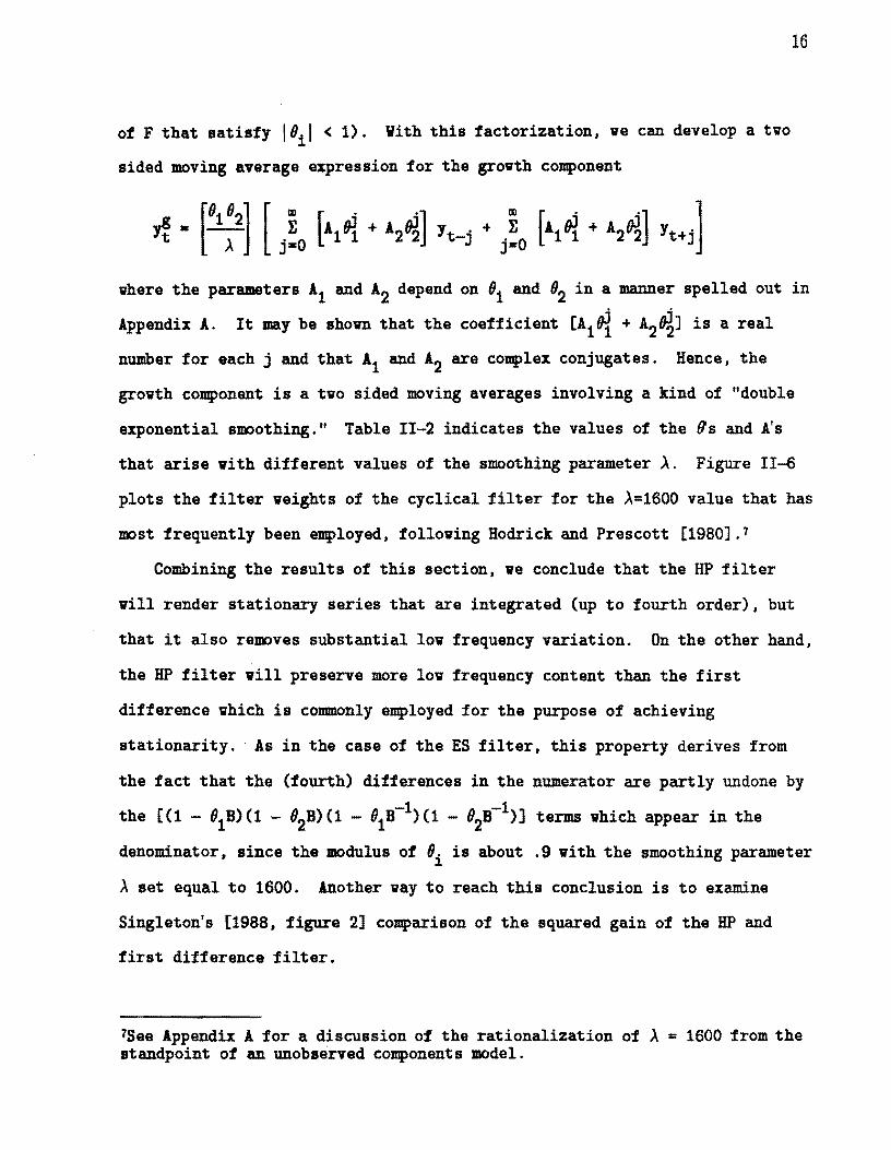
of F that satisfy 18i, < 1). With this factorization, we can develop a two

sided moving average expression for the growth component

where the parameters Al and A2 depend on 81 and 82 in a manner spelled out in

Appendix A. It may be shovn that the coefficient [A101 + A2~] is a real

number for each j and that Al and A2 are complex conjugates. Hence, the

growth component is a two sided moving averages involving a kind of "double

exponential smoothing." Table 11-2 indicates the values of the Os and A's

that arise with different values of the smoothing parameter A. Figure 11-6

plots the filter weights of the cyclical filter for the A=1600 value that has

most frequently been employed, following Hodrick and Prescott [1980] ,7

Combining the results of this section, we conclude that the HP filter

will render stationary series that are integrated (up to fourth order), but

that it also removes substantial low frequency variation. On the other hand,

the HP filter will preserve more low frequency content than the first

difference which is commonly employed for the purpose of achieving

stationarity .. As in the case of the ES filter, this property derives from

the fact that the (fourth) differences in the numerator are partly undone by

the [(1 - 81B)(1 - 82B) (1 - 81B-1)(1 - 8 B-1)] terms which appear in the2denominator, since the modulus of 8i is about .9 with the smoothing parameter

A set equal to 1600. Another way to reach this conclusion is to examine

Singleton's [1988, figure 2] comparison of the squared gain of the HP and

first difference filter.

7See Appendix A for a discussion of the rationalization of A = 1600 from the standpoint of an unobserved components model.

17

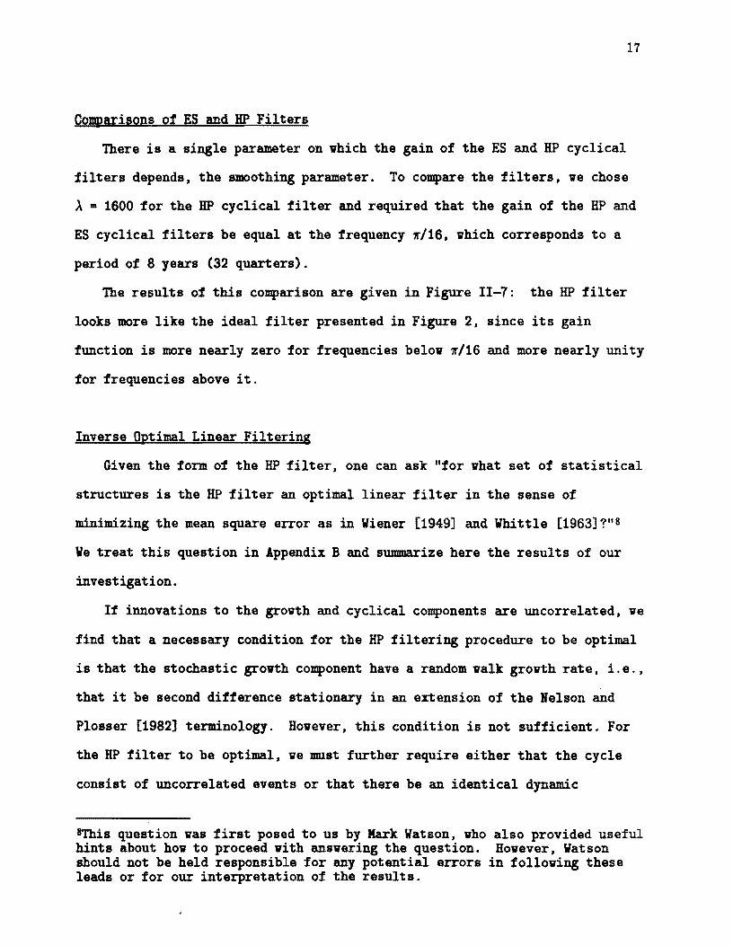
Comparisons of ES and HP Filters

There is a single parameter on vhich the gain of the ES and HP cyclical

filters depends. the smoothing parameter. To compare the filters. ve chose

A • 1600 for the HP cyclical filter and required that the gain of the HP and

ES cyclical filters be equal at the frequency ~/16. vhich corresponds to a

period of 8 years (32 quarters).

The results of this comparison are given in Figure 11-7: the HP filter

looks more like the ideal filter presented in Figure 2, since its gain

function is more nearly zero for frequencies belov ~/16 and more nearly unity

for frequencies above it.

Inverse Optimal Linear Filtering

Given the form of the HP filter. one can ask "for vhat set of statistical

structures is the HP filter an optimal linear filter in the sense of

minimizing the mean square error as in Wiener [1949] and Whittle [1963]1" 8

We treat this question in Appendix B and summarize here the results of our

investigation.

If innovations to the grovth and cyclical components are uncorrelated. ve

find that a necessary condition for the HP filtering procedure to be optimal

is that the stochastic grovth component have a random valk grovth rate, i.e.,

that it be second difference stationary in an extension of the Nelson and

Plosser [1982] terminology. Hovever. this condition is not sufficient. For

the HP filter to be optimal. ve must further require either that the cycle

consist of uncorrelated events or that there be an identical dynamic

trhis question vas first posed to us by Mark Watson. vho also provided useful hints about hov to proceed vith ansvering the question. Hovever. Watson should not be held responsible for any potential errors in folloving these leads or for our interpretation of the results.

18

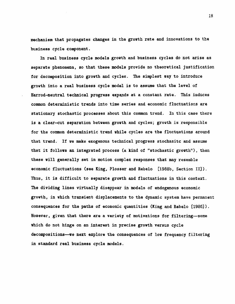
mechanism that propagates changes in the grovth rate and innovations to the

business cycle component.

In real business cycle models grovth and business cycles do not arise as

separate phenomena. so that these models provide no theoretical justification

for decomposition into grovth and cycles. The simplest vay to introduce

grovth into a real business cycle model is to assume that the level of

Harrod-neutral technical progress expands at a constant rate. This induces

common deterministic trends into time series and economic fluctuations are

stationary stochastic processes about this common trend. In this case there

is a clear-cut separation betveen grovth and cycles; grovth is responsible

for the common deterministic trend vhile cycles are the fluctuations around

that trend. If ve make exogenous technical progress stochasitc and assume

that it follovs an integrated process (a kind of "stochastic grovth"). then

these viII generally set in motion complex responses that may resemble

economic fluctuations (see King. Plosser and Rebelo [1988b, Section II]).

Thus. it is difficult to separate grovth and fluctuations in this context.

The dividing lines virtually disappear in models of endogenous economic

grovth. in vhich transient displacements to the dynamic system have permanent

consequences for the paths of economic quantities (King and Rebelo [1986]).

Hovever. given that there are a variety of motivations for filtering--some

vhich do not hinge on an interest in preCise grovth versus cycle

decompositions--ve next explore the consequences of lov frequency filtering

in standard real business cycle models.

19

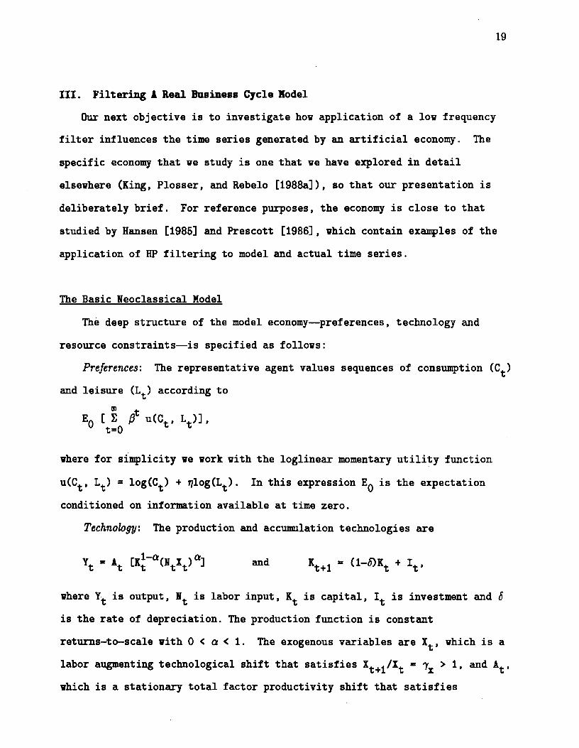
III. Filtering 1 Real Business Cycle Kodel

Our next objective is to investigate hov application of a lov frequency

filter influences the time series generated by an artificial economy. The

specific economy that ve study is one that ve have explored in detail

elsevhere (King, Plosser, and Rebelo [1988a]), so that our presentation is

deliberately brief. For reference purposes, the economy is close to that

studied by Hansen [1985] and Prescott [1986], vhich contain examples of the

application of HP filtering to model and actual time series.

The Basic Neoclassical Model

The deep structure of the model economy--preferences, technology and

resource constraints--is specified as follovs:

Preferences: The representative agent values sequences of consumption (Ct )

and leisure (L ) according tot (I) ;t;

EO [E P u(C , L )],t tt=O

vhere for simplicity ve vork vith the loglinear momentary utility function

u(Ct , L ) = 10g(C ) + ~log(Lt). In this expression EO is the expectationt t

conditioned on information available at time zero.

Technowgy: The production and accumulation technologies are

and

vhere Yt is output, Nt is labor input, Kt is capital, It is investment and 0

is the rate of depreciation. The production function is constant

returns-to-scale vith 0 < a < 1. The exogenous variables are Xt , vhich is a

labor augmenting technological shift that satisfies X +1/X = 1x > 1, and At't t

vhich is a stationary total factor productivity shift that satisfies

20

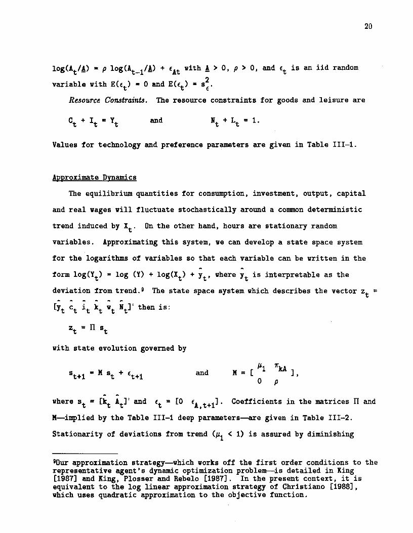
10g(At/A) • p log(A _1/A) + fAt vith A > 0, P > 0, and ft is an iid randomt

variable vith H(ft ) • 0 and H(ft ) • s~. Resource Constraints. The resource constraints for goods and leisure are

and

Values for technology and preference parameters are given in Table III-i.

Approximate Dynamics

The equilibrium quantities for consumption, investment, output, capital

and real vages viII fluctuate stochastically around a common deterministic

trend induced by It' On the other hand, hours are stationary random

variables. Approximating this system, ve can develop a state space system

for the logarithms of variables so that each variable can be vritten in the .. ..

form 10g(Yt ) = log (Y) + 10g(I ) + Yt' vhere Yt is interpretable as thet

deviation from trend. 9 The state space system vhich describes the vector Zt = A ..

[Yt it kt Nt]' then is:ct vt

vith state evolution governed by

""kAand M = [ Jl.l ], o P

.. .. vhere St = [kt At]' and ft· [0 fA, t+1]' Coefficients in the matrices II and

H--implied by the Table 111-1 deep parameters--are given in Table 111-2.

Stationarity of deviations from trend (Jl.l < 1) is assured by diminishing

80ur approximation strategy--vhich vorks off the first order conditions to the representative agent's dynamic optimization problem--is detailed in King [1987] and King, Plosser and Rebelo [1987]. In the present context, it is equivalent to the log linear approximation strategy of Christiano [1988], vhich uses quadratic approximation to the objective function.

21

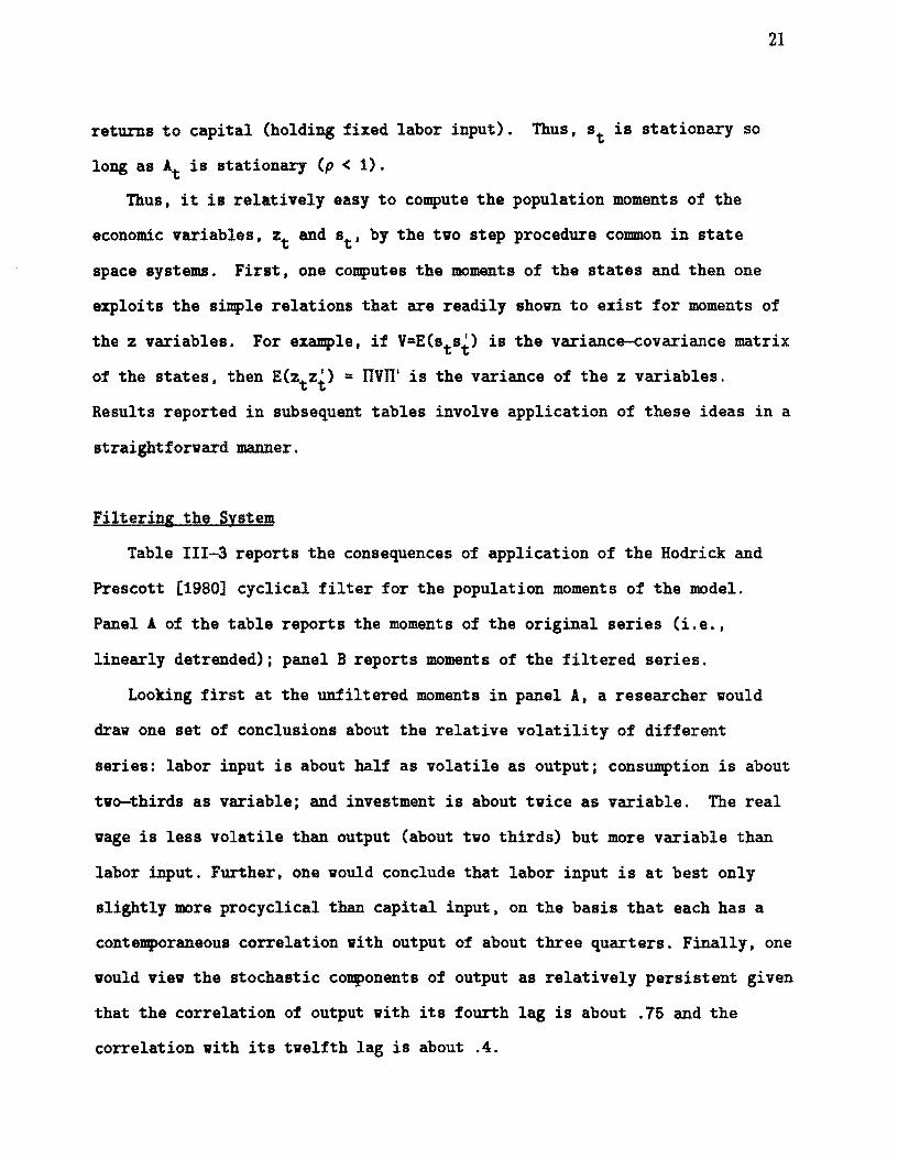
returns to capital (holding fixed labor input). Thus, St is stationary so

long as At is stationary (p < 1).

Thus, it is relatively easy to compute the population moments of the

economic variables, Zt and St' by the tvo step procedure common in state

space systems. First, one computes the moments of the states and then one

exploits the simple relations that are readily shovn to exist for moments of

the Z variables. For example, if V=E(sts~) is the variance-covariance matrix

of the states, then E(ZtZ~) = nvn' is the variance of the Z variables.

Results reported in subsequent tables involve application of these ideas in a

straightforvard manner.

Filtering the System

Table 111-3 reports the consequences of application of the Hodrick and

Prescott [1980] cyclical filter for the population moments of the model.

Panel! of the table reports the moments of the original series (i.e.,

linearly detrended)j panel B reports moments of the filtered series.

Looking first at the unfiltered moments in panel A, a researcher vould

drav one set of conclusions about the relative volatility of different

series: labor input is about half as volatile as outputj consumption is about

tvo-thirds as variable; and investment is about tvice as variable. The real

vage is less volatile than output (about tvo thirds) but more variable than

labor input. Further, one vould conclude that labor input is at best only

slightly more procyclical than capital input, on the basis that each has a

contemporaneous correlation vith output of about three quarters. Finally, one

vould viev the stochastic components of output as relatively persistent given

that the correlation of output vith its fourth lag is about .75 and the

correlation vith its tvelfth lag is about .4.

22

Turning nov to panel B, one finds the population moments for the

components of time series isolated by the HP cyclical filter, vith the

smoothing parameter A set to 1600. Through this filter, a very different

picture of business cycles emerges. Consumption is nov only about a quarter

as variable as output, labor input is tvo thirds as variable and investment

is nov nearly three times as variable. The volatility of the real vage is

only one sixth that of output. Further, vith an application of the HP

filter, the real vage it is sharply less volatile than labor input (only

about one half as volatile).

One nov also has a very different picture of cyclical movements in

inputs: labor input is very highly correlated vith output (.98) and capital

is unrelated to cyclical activity (its correlation is .07). Finally,

autocorrelation in output is close to zero at a lag of one year (four

quarters) and negative at a lag of three years (tvelve quarters).

Considering the state space system, it is not too hard to see vhat is

happening to produce these results. The evolution of all variables depends

on their veights placed on the state variables, the capital stock and the

technology shock. The technology shock is given by At = P A _1 + fAt' vhicht A m S

implies that it is representable as At = E P fA,t-s' Given the lav of . s=O

motion for capital, kt+1 = P1 kt + ~kA At vith P1~·95, the capital stock is a

moving average of technology shocks, vith veights that die out very slovly.

Relative to the technology shock, then, the capital stock is very slov moving

and application of the lov frequency filter down plays its influence and

raises that of the technology shock. Notice that this occurs despite the

fact that both capital and technology are driven by fAt' since they are

related to it by different (one sided) linear filters.

23

Figure 111-1 shovs the impact of HP filtering on the spectral densities

of these tvo variables (the dashed line is the spectral density of the

unfiltered series and the solid line is the spectral density of the filtered

series). Despite the fact that both variables display Granger's [1961]

typical spectral shape, the pover of the capital stock is more concentrated

at lov frequencies and, consequently, the HP filter dovnplays its relative

influence.

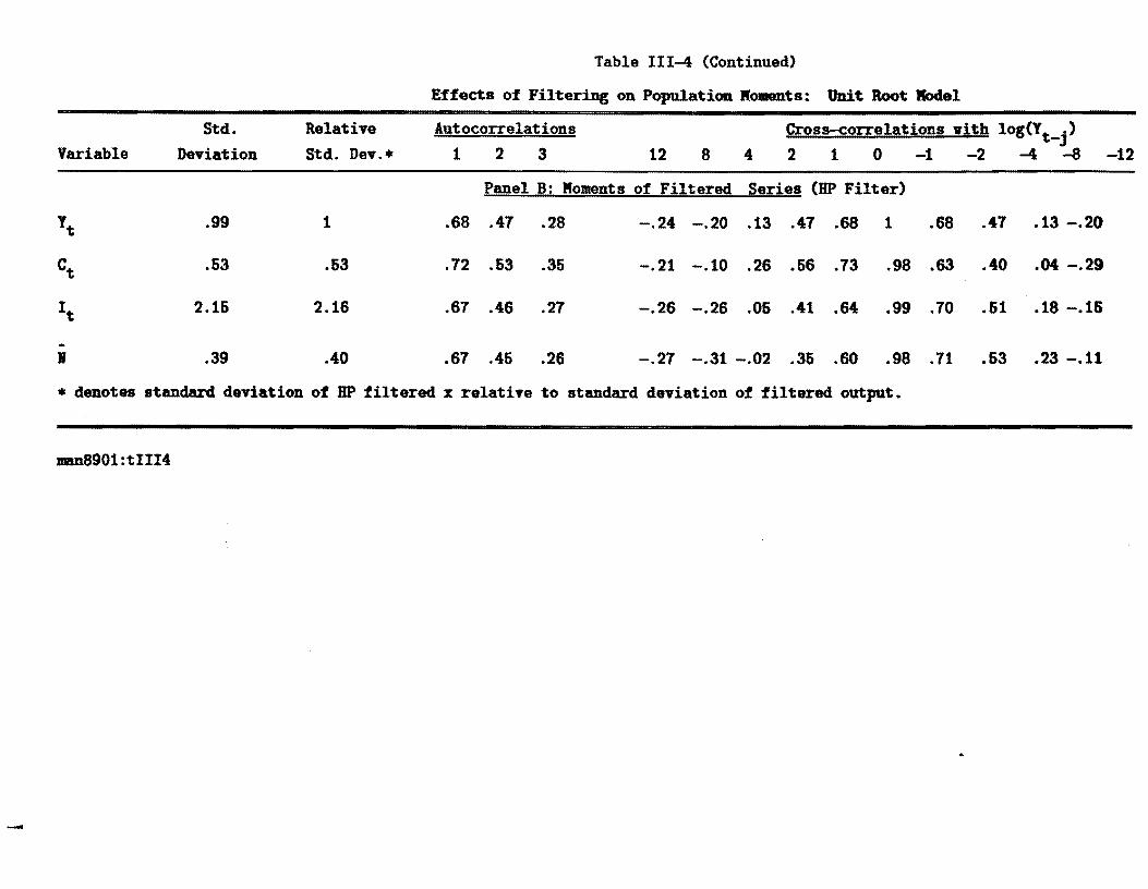
Random Walk Technology Shocks

It is possible to solve this model under the alternative assumption that

technology shocks are integrated processes (see Christiano [1988] or King,

Plosser and Rebelo [1988b, section 2]). In viev of the Nelson and Plosser

[1982] results and given the intuitive idea that technology shocks are veIl

modeled as a random valk (vith positive drift), ve present some final results

based on that alternative specification in Table 111-2. Since the levels of

variables are not stationary, population moments are not finite. Thus, ve

present results for the first difference filter and for the HP cyclical

filter. In the presence of this nonstationarity, the HP filter produces

results that broadly resemble those of Table III-3, alth~ugh the shift to a

random valk technology shoc~ does reduce the extent of labor volatility, as

stressed by Hansen [1988].

Does Filtering Affect Moments that Are Very Important?

In vieving the foregoing results, one is naturally led to ask vhether the

practice of filtering affects moments that are very important from the

standpoint of real business cycle research. In this research area, it is

established practice to focus on a subset of moments--typically

24

contemporaneous correlations and selected autocorrelations or cross

correlations--in evaluating vhether an alteration in a model's physical

environment is quantitatively important. For example, Hansen's [1985]

analysis of the influence of indivisibilities in labor supply on a real

business cycle model concentrates on its implications for the contemporaneous

covariance matrix of the model's variables, notably the relative volatility of

hours and productivity. Clearly, given the foregoing. HP filtering viII

alter the moments studied by Hansen. Hovever, no major alteration in one's

vievs of the importance of this structural Change is indicated by a careful

comparison of Hansen's [1986] analysis (vhich uses HP filtering) and King,

Plosser and Rebelo's [1988a] analysis of a similar economy (vhiCh does not

employ HP filtering).

By contrast, vith complicated model elements that are capitalistic in

nature--that is, those vhich alter intertemporal substitution

opportunities--HP filtering is likely to be far more important. To take one

example, Rouvenhorst [1988] studies the influence of the "time to build"

technology of Kydland and Prescott [1982]. He concludes that the major

differences betveen models vith and vithout time to build lie in the

autocovariances--vith jumps in othervise smooth generating functions

occurring at the lags that are integer multiples of the delay betveen the

initiation and fruition of an investment project. The application of a

smoothing procedure--such as the HP cyclical filter--vould likely mask this

key implication of the model. To take another example, there has been recent

interest in the cyclical implications of models vith endogenous long run

grovth (King and Rebelo [1986), King. Plosser and Rebelo [1988b) and

Christiano and Eichenbaum [1988b]). ! major feature of these models is the

endogenous generation of a stoChastic grovth component of the form that is

25

eliminated by the HP cyclical filter. Ve conclude that there are important

and numerous extensions of real business cycle models in vhich essential

information vill be lost if the HP cyclical filter is the unique mechanism

for vieving model implications.

IV. Implications of Our .lnalysis for Practice

To this point, ve have provided an exposition and critique of an

established practice in real business cycle research, the lov frequency

filtering of model and actual time series vith a method due to Hodrick and

Prescott [1980]. In our viev, this procedure has gained videspread

acceptance for three reasons, vhich are important background to our

recommendations for alterations of research practice. First, as stressed by

Hodrick and Prescott [1980, page 1], their method is a simple procedure that

can be mechanically applied to economic time series. This characteristic

reduces the judgmental decisions by a researcher and thus makes easier the

process of cross-investigation comparison vhich is essential to scientific

progress. Second, ve have seen that HP cyclical filtering renders stationary

series that have persistent changes in the underlying grovth rate. Thus, as

stressed by Hodrick and Prescott [1980, pp. 4-5], it is capable of

accoDDDOdating phenomena such as "the productivity slovdovn" in underlying

time series. Third, the procedure implements a traditional viev that

economic grovth and business cycles are phenomena that are to be studied

separately. Further, application of the HP procedure generates summary

statistics for real U.S. data that correspond to many economists' prior

notions of "business cycle facts."

Ve nov provide some suggestions for hov researchers should modify

practice based on the results of our investigation, so as to maximize

26

scientific communication. These suggestions are based on three ideas: (i) it

is desirable on statistical grounds to report sample moments only vhen time

series have finite population counterparts; (ii) economic models generally

contain explicit instructions about hov to transform the data so that it viII

be stationary; and (iii) since the traditional separation of grovth and

business cycles is not an attribute of modern dynamic equilibrium the~ries,

vhich embody concrete and extensive cross frequency restrictions, economists

pursuing the real business cycle research program cannot have sharp priors

about the decomposition of macroeconomic time series along these lines.

Reporting Attributes of Dynamic Macroeconomic Models: The moment

implications of a dynamic equilibrium model are governed by its reduced form,

e.g., the linear dynamic system summarized by the IT and M matrices.

Investigators should alvays report sufficient information for calculation of

alternative moment implications to be undertaken by another researcher

vithout solution of the model. 10

Reporting HP Growth Components: Researchers utilizing the HP filtering

procedure should report moments of the actual and model generated "stochastic

grovth" components so that comparisons betveen models can be made on the

basis of this information.

First, since the "prior fl under the HP filtering procedure is that the

actual data contain a stochastic trend, a transformation to achieve

stationarity is necessary. Belov, ve report results for the HP stochastic

10Although not present in such important contributions as Kydland and Prescott [1982], Hansen [1986], and Prescott [1986], this information is provided in other early vork by Kydland and Prescott [1979] and Long and Plosser [1983J. More recently, this practice is folloved by Christiano [1988], Hansen and Sargent [1988], King, Plosser and Rebelo [1988a,b], and Kydland and Prescott [1988] in the recent Journal of Monetary Economics special issue on Real Business Cycles.

27

growth component extracted from a model filtered with (l-B) (1-B-1)/2 for this

purpose. Ve have experimented with this centered second difference for two

reasons: (i) it induces no phase shift; and, (ii) it renders stationary a

time series with a random walk growth rate.

Second, the researcher should report statistics on this stochastic growth

component under the transformation implied by the specified dynamic economic

JlK)del that naturally achieves stationarity: we give two examples of this

transformation below.

Reporting Moments for Model Based Data Transformations: Dynamic stochastic

economic models generally suggest ways of treating nonstationarity in

economic time series. Any investigation should at minimum report the direct

transformations suggested by the model, since evidence against this

transformation is useful in judging the adequacy of the model.

Trend Stationary Models: For example, one common model building strategy

is to view economic time series as stationary relative to a common

deterministic trend, as is implicit in Hansen [1985] and explicit in King,

Plosser and Rebelo [1988a]. Under this scenario, our results suggest that HP

filtering can dramatically alter how a researcher views a model economy as

working, for example in terms the relative importance of variation in capital

and labor in response to persistent but stationary technology shocks. Major

components of time series on output, consumption etc. are treated by the

filter as stochastic growth, when the posited model involves none. Ve

recommend two alterations in practice for this case. First. researchers

should report unfiltered moment implications as well as HP filtered moment

implications. Researchers using the HP filter should also report attributes

of the isolated stochastic growth components. under the model's assumption

that these are stationary and the alternative assumption that there is a

28

random walk growth rate, which is implicit in analysis underlying HP

filtering. In table IV.l, we provide an application of these methods to the

population moments of the model economy described in section III above. These

tables make clear that there is a substantial component of the time series

removed by the HP filter and that this component in many ways resemble those

of the unfiltered series. Thus, in such a trend stationary model, a much

clearer picture of the operation of the theoretical model is provided by

table 111-3, panels AlB, and table IV-l, panels AlB, than by individual

components. 11

Presumably, it is not feasible to report all of the information in the

tables we have presented here, given constraints on journal space. But it

would be very easy to add information on HP growth components to our table

1-1, which is a standard device for reporting implications of business cycle

models.

Stochastic Trend Models: Frequently, low frequency filtering is

motivated by concern over potential nonstationarity of macroeconomic time

series as suggested, for example, by lelson and Plosser's [1982] investigation

of individual series and King, Plosser, Stock and Watson's [1987]

investigation of common stochastic trends. For models with explicit

stochastic growth elements--as in, for example, Christiano [1988], Hansen

[1988] and King, Plosser and Rebelo [1988b]----it will generally not be

meaningful to produce simulated moments for the levels of economic variables,

since the population counterparts are not finite. Some transformation of

llFurther, in such trend stationary environments, we caution that research which focuses on dynamic elements of model construction----like that of Rouwenhorst (1988) discussed earlier--should be wary of interpreting HP filtered moments as providing much information about the importance of structural changes.

29

actual and model generated data viII be necessary: tvo natural

transformations that are consistent vith the economic structure of stochastic

steady state models are first differencing and construction of ratios of

variables possessing common stochastic trends. Motivated by concern over

nonstationarity. some recent investigations do undertake exploration of model

sensitivity to filtering and data transformation in the vay that our

investigation suggests. Examples are provided in Christiano and Eichenbaum

[1988a], vho explore HP filtering and first differencing. and King, Plosser

and Rebelo [1988b], vho use first difference filtering and a ratio form that

involves imposition of a common stochastic trend. Again, for researchers

using HP filtering. our recommended practice requires reporting of statistics

on stochastic grovth components under (i) the model based assumption that the

first difference is stationary and (ii) using the second difference filter

discussed earlier.

10 real business cycle research to this point has explicitly incorporated

the persistent Changes in productivity grovth originally cited by Hodrick and

Prescott [1980] as a major motivation for application of their filter to post

var U.S. data. This feasible investigation could veIl shed further light on

the interaction of grovth and business cycles.

V. Su.aary and Conclusions

This paper has reported on implications of lov frequency filtering.

focusing on the HP filter--due to Hodrict and Prescott [1980]--vhich is

commonly used in investigations of the stochastic properties of real business

cycle models.

First, application of the filter to U.S. real gross national product and

a measure of labor input illustrates the impact of HP filtering on the

30

character of cyclical components. Second, ve derive convenient expressions

for the HP filter and the closely related exponential smoothing (ES) filter

in forms appropriate for both the time domain and frequency domain. These

results are used (i) to discuss the influence of smoothing parameters and

(ii) to demonstrate that the cyclical components vhich these filters generate

are stationary, vhen the underlying time series are differenced stationary

stochastic processes in the sense of Belson and Plosser [1982]. Third, ve

consider the conditions under vhich the HP filter is the optimal linear

filter in the sense of Wiener [1949] and Whittle [1963]. These conditions

are unlikely to be even approximately true in practice. Fourth, application

of the HP filter to a basic real business cycle model demonstrates that this

filter substantially influences the perception of the operation of the model

economy, as vieved by researchers studying its moment implications. Fifth,

based on the results of our investigations. ve recommend some nev practices

designed to facilitate scientific communication betveen researchers.

At the end of our investigation. hovever, ve remain struck by the

Figures presented in section 1: macroeconomic research focusing on the

component of the time series that is isolated by the HP cyclical filter--in

terms of either devising stylized facts or evaluating dynamic economic

models--is likely to capture only a subset of the time series variation that

most economists associate vith cyclical fluctuations. A major facet of our

ongoing research is the construction of dynamic models that more completely

integrate the explanation of these components.

31

References

Baxter, Marianne, [1988] "Business Cycles and the Exchange Rate Regime: Some Evidence from the United States," Rochester Center for Economic Research vorking paper #169.

Baxter, Marianne and Alan Stockman, [1988] "Business Cycles and the Exchange Rate Regime: Some International Evidence," forthcoming in Journal of Monetary Economics, September 1989.

Bell, W., [1984] "Signal Extraction for Non-Stationary Time Series,lI Annals of Statistics 12, 646-684.

Brovn, R., [1962] Smoothing. Forecasting and Prediction of Discrete Time Series. Prentice Hall, Englevood Cliffs, Nev Jersey.

Burns, Arthur and Wesley C. Kitchell, [1941] Measuring Business Cycles, Nev York, National Bureau of Economic Research.

Christiano, Lavrence, [1988] "Why does Inventory Investment Fluctuate So Much?" Journal of Monetary Economics, 21, No. 2/3, 247-280.

Christiano, Lavrence and Martin Eichenbaum, [1988a] "Is Theory Really Ahead of Business Cycle Measurement?" National Bureau of Economic Research vorking papers, # 2700.

Christiano, Lavrence and Martin Eichenbaum, [1988b] IIHuman Capital, Endogenous Gr9vth, and Aggregate Fluctuations,lI Northvestern University vorking paper.

Fishman, George, [1969] Spectral Methods in Econometrics, Cambridge, Harvard University Press.

Friedman, Milton, [1957] A Theory of the Consumption Function, Princeton, N.J.: Princeton University Press

Granger, Clive, [1961] "The Typical Spectral Shape of An Economic Variable," Econometrica, vol 37, no. 3, pp. 424-438.

Hansen, Gary, [1985] "Indivisible Labor and the Business Cycle," Journal of Monetary Economics 16, 309-27.

Hansen, Gary, [1988] "Technical Progress and Aggregate Fluctuations". U.C.L.A. vorking paper.

Hansen, Gary, and Thomas J. Sargent, [1988] "Straight Time and Over Time in General Equilibrium," Journal of Monetary Economics 21:2/3, 281-308.

Harvey, Andrev, [1981] Time Series Models. Oxford: Phillip Allan.

32

Hodrick, Robert and Edvard Prescott, [1980] "Post-War U.S. Business Cycles: An Empirical Investigation," working paper, Carnegie-Mellon University.

King, Robert G. and Charles I. Plosser, [1989] "Real Business Cycles and the Test of the Adelmans," University of Rochester.

King, Robert G., C. I. Plosser and S. T. Rebelo, [1988a] "Production, Grovth, and Business Cycles: I. The Basic Neoclassical Model," Journal of Monetary Economics 21:2/3, 196-232.

King, Robert G., C. I. Plosser and S. T. Rebelo, [1988b] "Production, Growth,and Business Cycles: II. Nev Directions," Journal of Monetary Economics 21:2/3, 309-342.

King, Robert G., C. I. Plosser and S. T. Rebelo, [1987] "Production, Grovth, and Business Cycles: Technical Appendix," University of Rochester manuscript.

King, Robert, Charles Plosser, James Stock, and Mark Watson, [1987] "Stochastic Trends and Economic Fluctuations,1I Rochester Center for Economic Research Working Paper #79.

King, Robert G. and Sergio. T. Rebelo, [1986] "Business Cycles vith Endogenous Grovth," University of Rochester manuscript.

Koopmans, Leonid, [1974] The Spectral Analysis of Time Series, Hev York: Academic Press.

Kuznets, Simon, [1930] Secular Movements in Production and Prices, Boston: Houghton Mifflin.

Kuznets, Simon, [1961], Capital and the American Economy: Its Formation and Financing, National Bureau of Economic Research.

Kydland, Finn and Edvard Prescott, [1979] "! Competitive Theory of Fluctuations and the Feasibility and Desirability of Stabilization Policy," in S • Fischer, ed. t Rational Expectations and Economic Policy, Chicago: University of Chicago Press.

Kydland, Finn and Edward Prescott, [1982] "Time to Build and Aggregate Fluctuations," Econometrica 60, 1346-70.

Kydland, Finn and Edvard Prescott, [1988], "The Work Week of Capital and Its Cyclical Implications," Journal of Monetary Economics, 21:2/3, 343-360.

Long, John and Charles Plosser, [1983] "Real Business Cycles," JOurnal of Political Economy 91, 1346-70.

McCallum, Bennett, [1989] "Real Business Cycles," in Robert Barro (ed.), Handbook of Modern Business Cycle Theory, Nev York: Wiley.

Mitchell, Wesley C., [1927] Business Cycles: The Problem and Its Setting, Jev York: National Bureau of Economic Research.

33

Mitchell, Wesley C., [1951] What Happens During Business Cycles, Neq York, Bational Bureau of Economic Research.

Belson, Charles and Charles Plosser, [1982] "Trends and Random Walks in Macroeconomic Time Series," Journal of Monetary Economics 10, 139-67.

Prescott, Edvard, [1986] "Theory .Ahead of Business Cycle Measurement, II Carnegie-Rochester Conference Series on Public Policy 25, 11-66.

Rouvenhorst, Geert, [1988] "Time to Build and Aggregate Fluctuations: A Reconsideration," University of Rochester, processed manuscript

Singleton, Kenneth, [1988] "Econometric Issues in the Analysis of Equilibrium Business Cycle Models," Journal of Monetary Economics, 21, 361-386.

Watson, Mark, [1986], "Univariate Detrending Methods vith Stochastic Trends," Journal of Monetary Economics, 18, 49-76.

Whittle, Peter, [1963] Prediction and Regulation, Princeton, B.J.: Van Nostrand.

Wiener, Norbert, [1949] Extrapolation. Interpolation and Smoothing of Stationary-Time-Series, Neq York: J. Wiley I Sons.

Appendix A

Analysis of the BP Filter in Time Domain

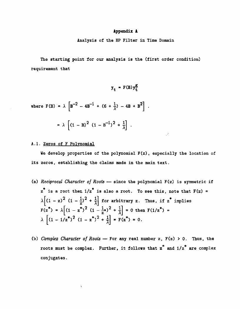
The starting point for our analysis is the (first order condition)

requirement that

Yt .. F(B)Y~

A.l. Zeros of F Polynomial

We develop properties of the polynomial F(z), especially the location of

its zeros, establishing the claims made in the main text.

(a) Reciprocal Character of Roots - since the polynomial F (z) is symmetric if

z· is a root then lIz· is also a root. To see this, note that F(z) = A[(l - z)2 (1 - ~)2 + i] for arbitrary z. Thus, if z· implies

• [ • 2 1 2 1] •F(z ) = A (1 - z) (1 -~) + X = 0 then F(l/z ) =

A [(1 - lIz)• 2 (1 - z)• 2 + X1] .. F(z ) • =o.

(b) Complex Character of Roots - For any real number z, F(z) > O. Thus, the

roots must be complex. Further, it follovs that z· and lIz· are complex

conjugates.

2

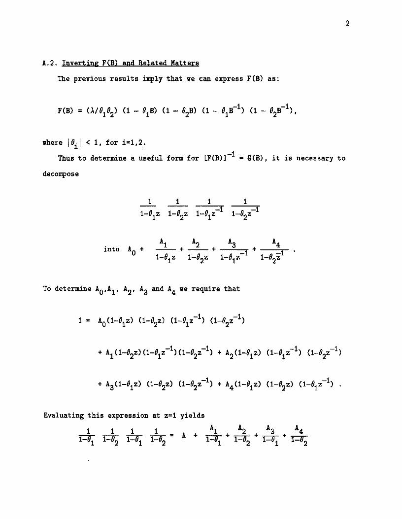
A.2. InvertingF(B) and Related Matters

The previous results imply that ve can express F(B) as:

vhere IlJil < 1, for i=1,2.

Thus to determine a useful form for [F(B)]-l = G(B), it is necessary to

decompose

1

into AO +

Evaluating this expression at z=l yields

1 1 1 1 _ Al A2 A3 A 4 fL' ':4IJ ':4IJ ':4IJ - A + ~ + ~ + 'T""""7J"""" + 'T""""7J"""".&.-11 .&.-11 .&.-11 .&.-11 .&.-11 .1-112 .&.-11 .&.-111 2 1 2 1 1 2

3

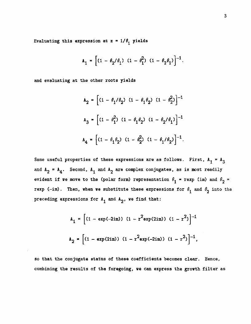
Evaluating this expression at z • 1/91 yields

and evaluating at the other roots yields

Some useful properties of these expressions are as follovs. First, Al =A3

and A2 = A4 , Second, Al and A2 are complex conjugates, as is most readily

evident if ve move to the (polar fornU representation 01 = rexp (im) and 02 =

rexp (-im). Then, vhen ve substitute these expressions for 01 and 02 into the

preceding expressions for Al and A2, ve find that:

so that the conjugate status of these coefficients becomes clear. Hence,

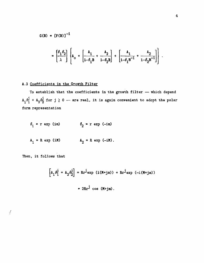
combining the results of the foregoing, ve can express the grovth filter as

4

G(B) • [F(B)]-l

A.3 Coefficients in the Growth Filter

To establish that the coefficients in the growth filter -- which depend

A1~ + A2~ for j ~ 0 -- are real, it is again convenient to adopt the polar

form representation

(J1 = r exp Urn) (J2 = r exp (-im)

A1 = R exp (iM) A2 =R exp (-iM).

Then, it follows that

= 2Rrj cos (M+jrn).

(

5

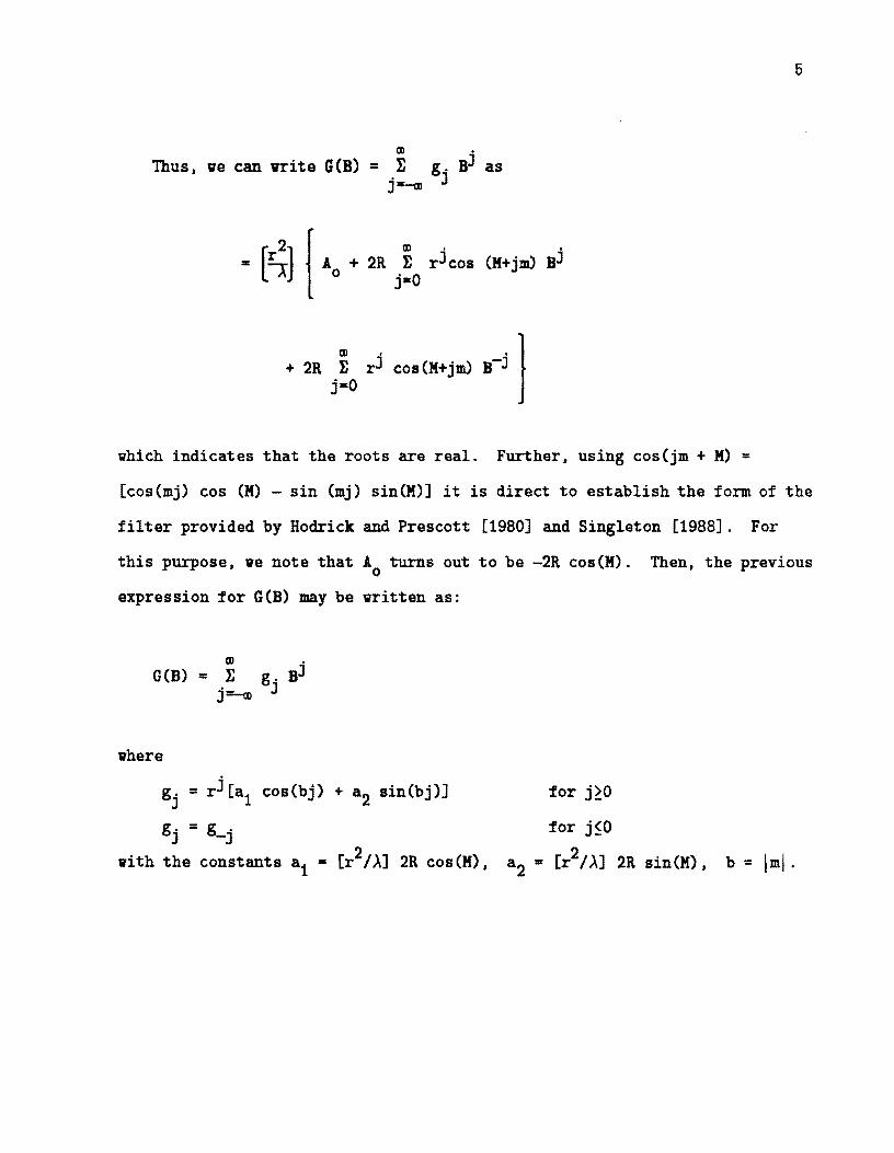
Thus, ve can vrite G(B) = E g. Bj as j=-m J

= [s]2

+ 2R E ~ cos (H+jm) B-j } j=O

vhich indicates that the roots are real. Further, using cos(jm + H) =

[cos(mj) cos (H) - sin (mj) sin(H)] it is direct to establish the form of the

filter provided by Hodrick and Prescott [1980] and Singleton [1988]. For

this purpose, ve note that Ao turns out to be -2R cos(H). Then, the previous

expression for G(B) may be vritten as:

III

G(B) = E g. Bj j=-m J

vhere

gj =r j [a1 cos(bj) + a2 sin(bj)] for j~O

gj = g-j for j~O

vith the constants a1 = [r2/A] 2R cos (H) , = [r2/A] 2R sin(H) , b = Iml.a2

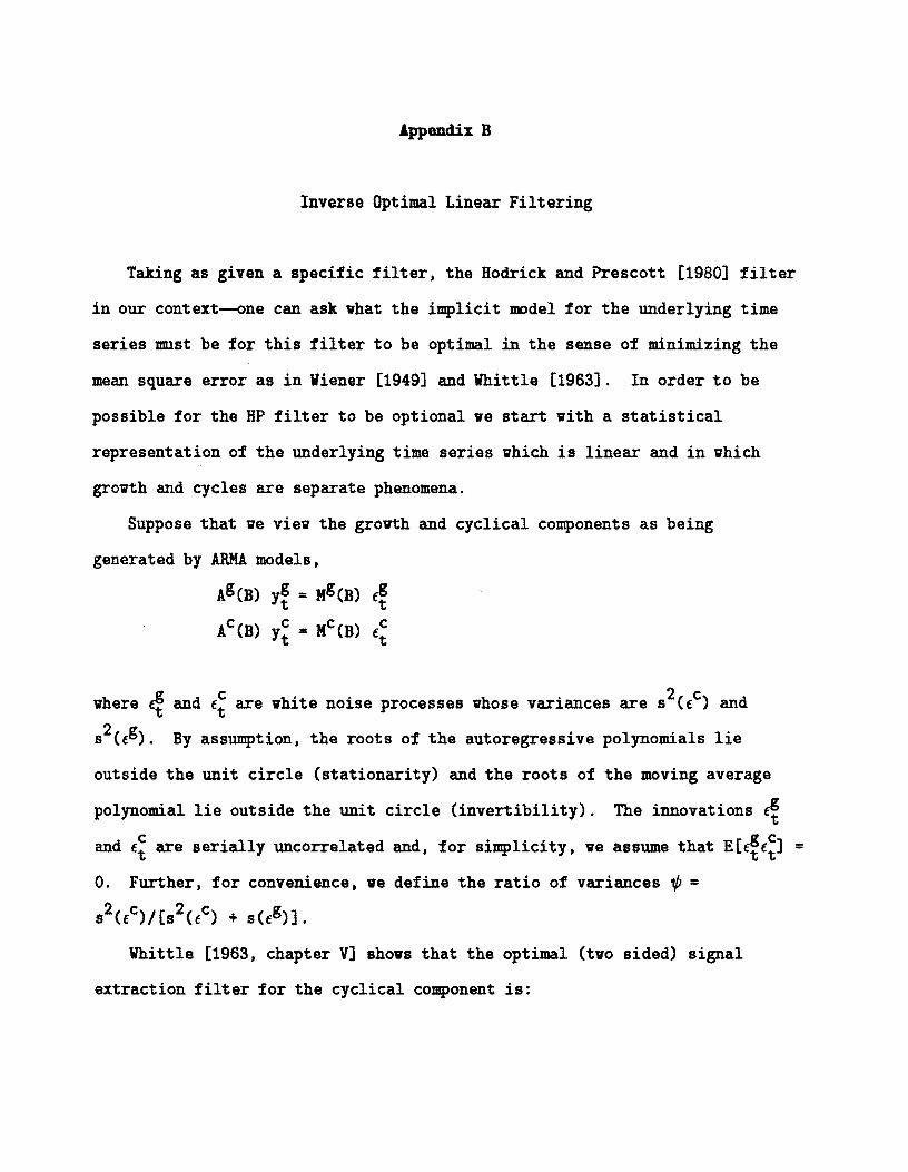
Appendix B

Inverse Optimal Linear Filtering

Taking as given a specific filter, the Hodrick and Prescott [1980] filter

in our context--one can ask vhat the implicit model for the underlying time

series must be for this filter to be optimal in the sense of minimizing the

mean square error as in Wiener [1949] and Whittle [1963]. In order to be

possible for the HP filter to be optional ve start vith a statistical

representation of the underlying time series vhich is linear and in vhich

grovth and cycles are separate phenomena.

Suppose that ve viev the grovth and cyclical components as being

generated by ARMA models,

AgeB) y~ = MgeB) f~

ACeB) y~ =MC(B) f~

vhere ~ and f~ are vhite noise processes vhose variances are s2(ec) and

S2(fg). By assumption, the roots of the autoregressive polynomials lie

outside the unit circle (stationarity) and the roots of the moving average

polynomial lie outside the unit circle (invertibility). The innovations f~

and f~ are serially uncorrelated and, for simplicity, ve assume that E[e~f~] =

O. Further, for convenience, ve define the ratio of variances 1/J =

S2(fC)/[s2(fc) + s(eg)].

Whittle [1963. chapter V] shovs that the optimal (tvo sided) signal

extraction filter for the cyclical component is:

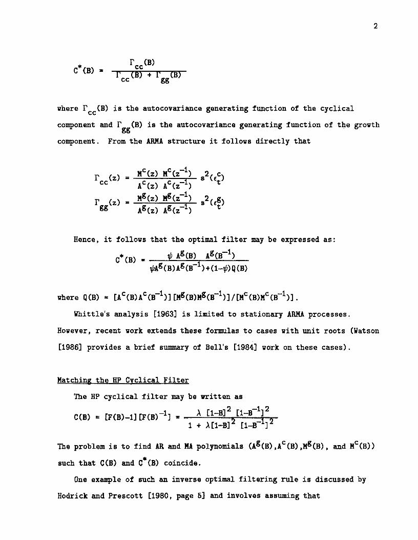
2

(B) + rC*(B) = r (B)cc gg

vhere rcc(B) is the autocovariance generating function of the cyclical

component and rgg(B) is the autocovariance generating function of the grovth

component. From the ARM! structure it follovs directly that

XC(z) XC(z-l)rcc(z) = S2(f~)

ACCz) ACCz-1) xg(z) XgCz-1)

rggCz) = s2Cf~)Ag(z) AgCz-1)

Hence, it follovs that the optimal filter may be expressed as:

1C*CB) = ¢ AgCB) AgCB- ) ¢Ag(B)AgCB-1)+(1-¢)QCB)

Whittle's analysis [1963] is limited to stationary ARMA processes.

Hovever, recent vork extends these formulas to cases vith unit roots (Watson

[1986] provides a brief summary of Bell's [1984] vork on these cases).

Xatching the HP Cyclical Filter

The HP cyclical filter may be written as

C(B) = [F(B)-l] [F(B)-l] = A [1_B]2 [1_B-1]2

1 + A[1-B]2 [1-8-1]2

The problem is to find AR and KA polynomials (Ag(B),Ac(B),Xg(B). and XCCB»

such that C(B) and C*(B) coincide.

One example of such an inverse optimal filtering rule is discussed by

Hodrick and Prescott [1980, page 6] and involves assuming that

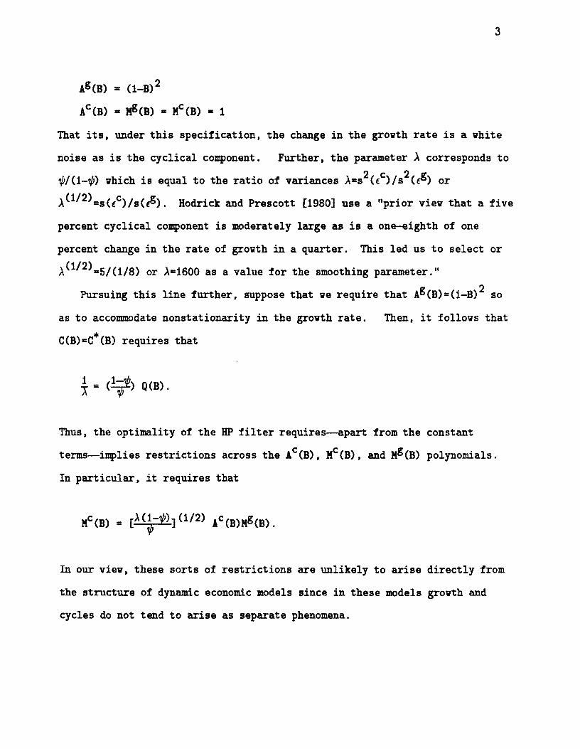
3

Ag(B) • (1_B)2

AC(B) • Hg(B) = HC(B) = 1

That its. under this speci1ication. the change in the grovth rate is a vhite

noise as is the cyclical component. Further, the parameter A corresponds to

~/(1-~) vhich is equal to the ratio of variances A.s2(fc)/s2(~) or

A(1/2)=s(fc)/s(~). Hodrick and Prescott [19S0] use a "prior viev that a five

percent cyclical component is moderately large as is a one-eighth of one

percent change in the rate of grovth in a quarter. This led us to select or

A(1/2)=5/(1/S) or A=1600 as a value for the smoothing parameter."

Pursuing this line further, suppose that ve require that Ag(B)=(1-B)2 so

as to accommodate nonstationarity in the grovth rate. Then, it fo110vs that

C(B)=C*(B) requires that

i = (1~) Q(B).

Thus, the optimality of the HP filter requires--apart from the constant

terms--imp1ies restrictions across the AC(B) , HC(B), and Hg(B) polynomials.

In particular, it requires that

In our viev, these sorts of restrictions are unlikely to arise directly from

the structure of dynamic economic models since in these models grovth and

cycles do not tend to arise as separate phenomena.

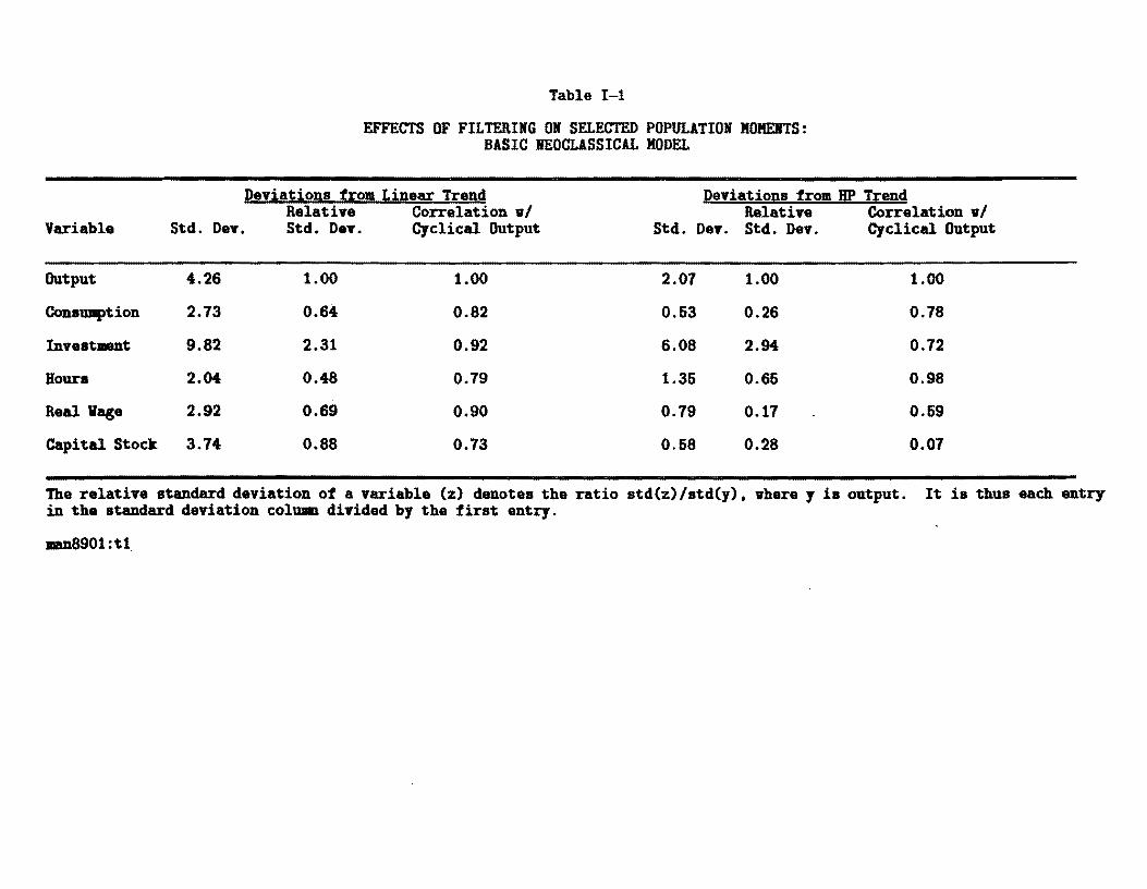
Table 1-1

EFFECTS OF FILTERING ON SELECTED POPULATION MOMENTS: BASIC NEOCLASSICAL MODEL

Deyiations from Linear Trend DeYiations from HP Trend RelatiYe Correlation vI RelatiYe Correlation vI

Variable Std. Dey. Std. Dey. Cyclical Output Std. Dey. Std. Dey. Cyclical Output

Output 4.26 1.00 1.00 2.01 1.00 1.00

Cons1Dlption 2.73 0.64 0.82 0.53 0.26 0.78

InYestMnt 9.82 2.31 0.92 6.08 2.94 0.72

Hours 2.04 0.48 0.19 1.35 0.65 0.98

Real Vage 2.92 0.69 0.90 0.19 0.17 0.59

Capital Stock 3.74 0.88 0.73 0.58 0.28 0.07

The relative standard deviation of a variable (z) denotes the ratio std(z)/std(y), vhare y is output. It is thus each entry in the standard deviation column divided by the first entry.

man8901 :t 1.

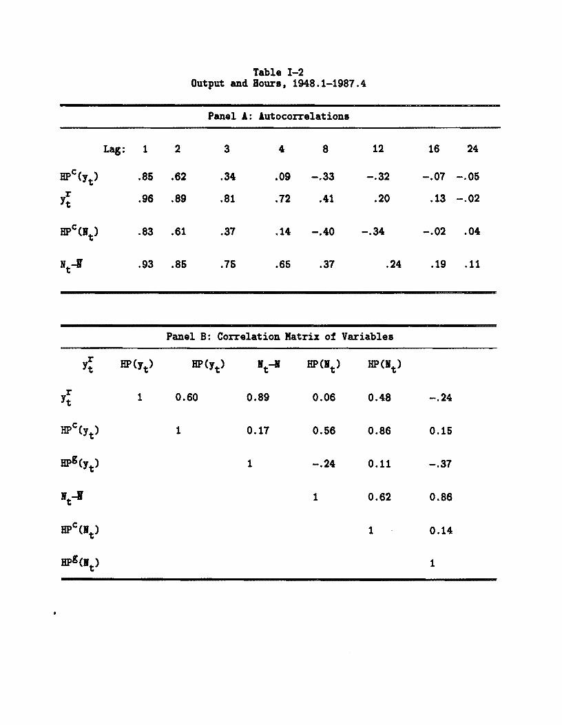
Table 1-2 Output and Hours, 1948.1-1987.4

Panel A: Autocorrelations

Lag:

HPcCYt )

Y~

1

.86

.96

2

.62

.89

3

.34

.81

4

.09

.72

8

-.33

.41

12

-.32

.20

16

-.07

.13

24

-.06

-.02

HPcClt

) .83 .61 .37 .14 -.40 -.34 -.02 .04

Nt-l .93 .86 .76 .66 .37 .24 .19 .11

Panel B: Correlation Matrix of Variables

Y~ HP(Yt ) HP(Yt ) I t - ­HP(lt ) HPClt )

rYt 1 0.60 0.89 0.06 0.48 -.24

HPc(Yt ) 1 0.17 0.66 0.86 0.16

HPgCyt

) 1 -.24 0.11 -.37

It-I 1 0.62 0.86

HPcClt

) 1 0.14

HPgclt ) 1

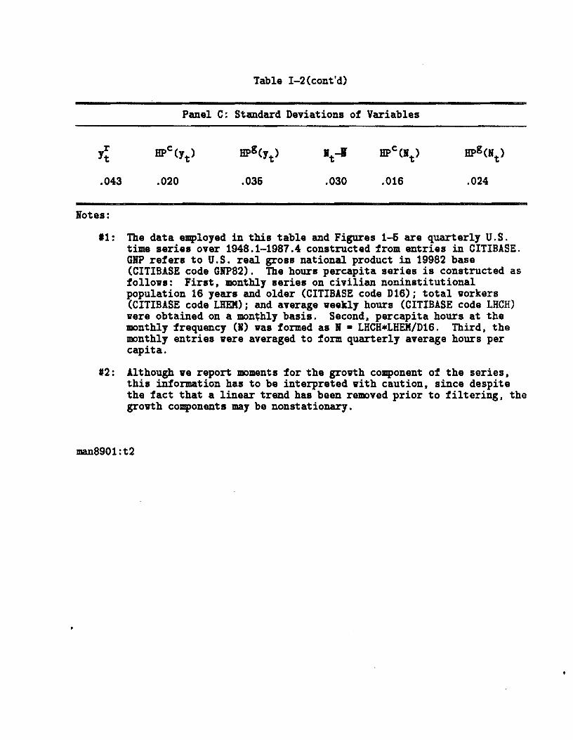
Table 1-2 (cont'd)

Panel C: Standard Deviations of Variables

.043

lotes:

'1: The data employed in this table and Figures 1-5 are quarterly U. S . time series over 1948.1-1987.4 constructed from entries in CITIBASE. GIP refers to U.S. real gross national product in 19982 base (CITIBASE code GIP82). The hours percapita series is constructed as follovs: First, monthly series on civilian noninstitutional population 16 years and older (CITIBASE code D16); total vorkers (CITIBASE code LHEK); and average veekly hours (CITIBASE code LHCH) vere obtained on a mon~hly basis. Second, percapita hours at the monthly frequency (I) vas formed as I • LHCH*LHEM/D16. Third, the monthly entries vere averaged to form quarterly average hours percapita.

#2: Although ve report moments for the grovth component of the series, this information has to be interpreted vith caution, since despite the fact that a linear trend has been removed prior to filtering, the grovth components may be nonstationary.

man8901:t2

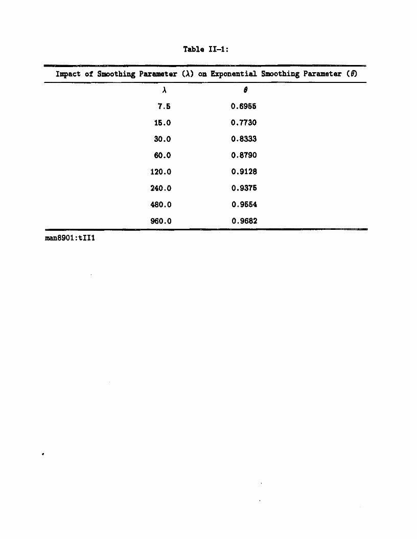
Table 11-1:

Impact of Smoothing Parameter C\) on Exponential Smoothing Parameter (6)

A

7.5

15.0

30.0

60.0

120.0

240.0

480.0

960.0

, 0.6955

0.7730

0.8333

0.8790

0.9128

0.9375

0.9554

0.9682

man8901:tII1

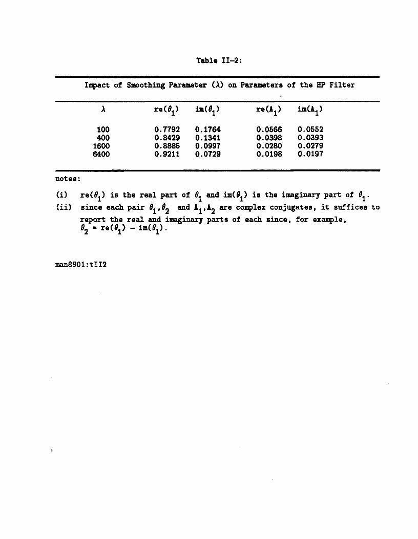
Table 11-2:

Impact of Smoothing Parameter (~) on Parameters of the HP Filter

100 400

1600 6400

re( '1)

0.7792 0.8429 0.8885 0.9211

ilI(81 )

0.1764 0.1341 0.0997 0.0729

re(1 )1

0.0566 0.0398 0.0280 0.0198

ilI(1 )1

0.0552 0.0393 0.0279 0.0197

notes!

(i) re(81) is the real part of 81 and im('1) is the imaginary part of 81, (ii) since eaCh pair 81,82 and 11,12 are complex conjugates, it suffices to

report the real and imaginary parts of eaCh since, for example, f)2 • re(81) - im«()1)'

ma.n8901:tII2

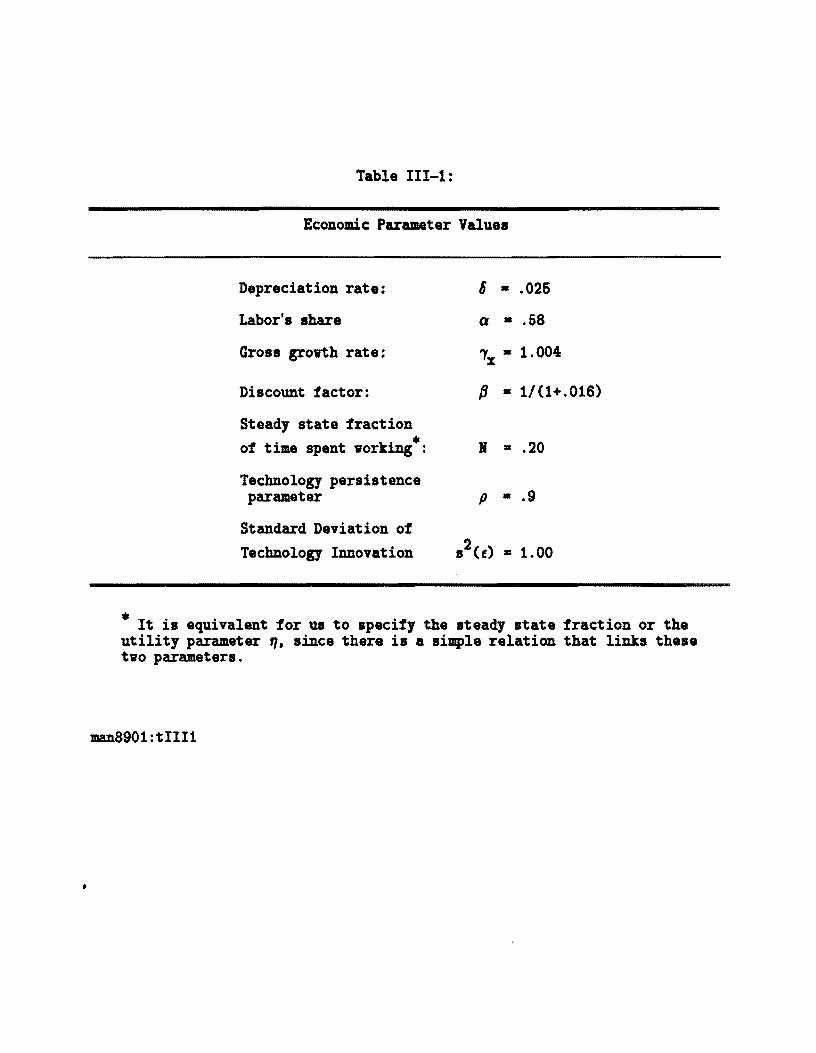
Table 111-1:

ECODOmiC Parameter Values

DepreciatioD rate:

Labor's share

Gross growth rate:

Discount factor:

Steady state fractioD of time speDt vorking*:

Technology persisteDce parameter

Standard DeviatioD of Technology InnovatioD

6 • .026

a • .68

7;x • 1.004

p • 1/(1+.016)

I • .20

p • .9

* It is equivalent for us to specify the steady state fractioD or the utility parameter q. since there is a simple relatioD that links these tvo parameters.

man8901:tIII1

•

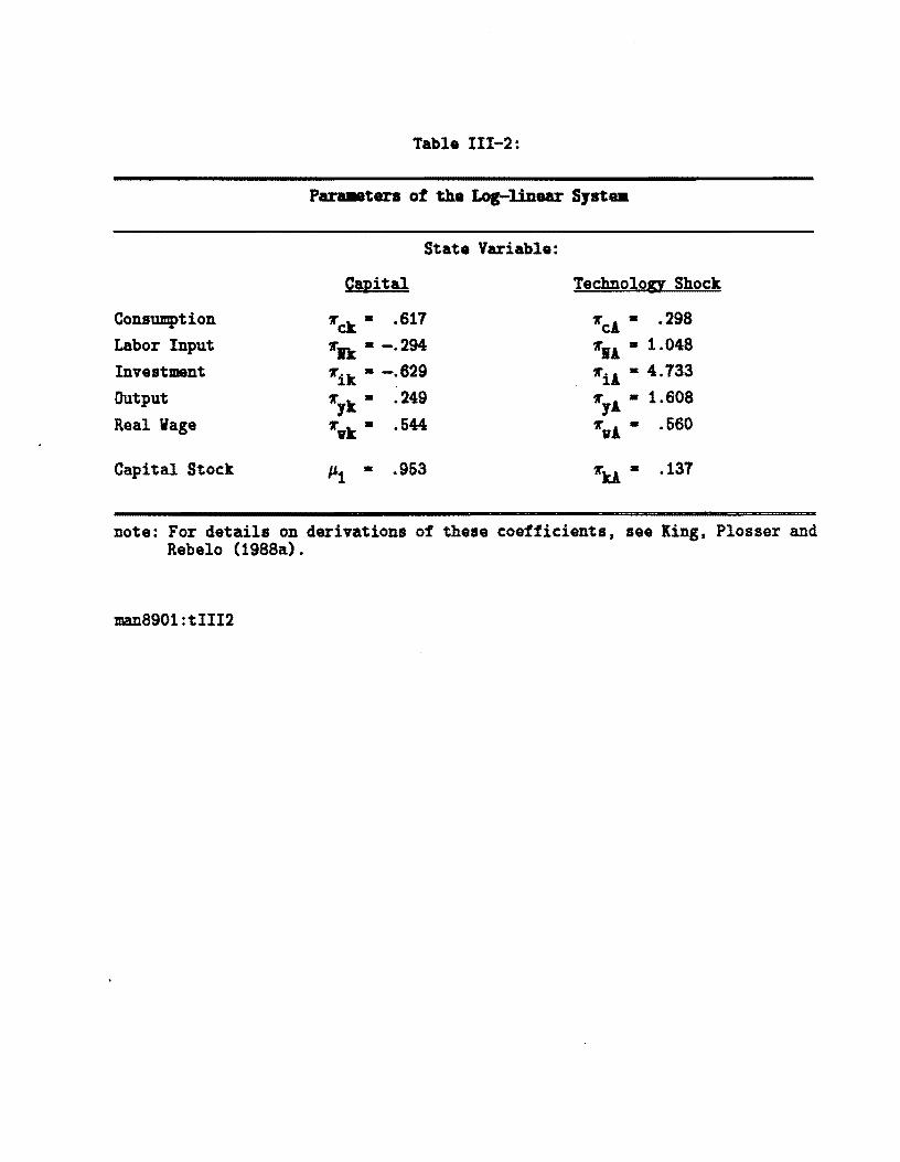
Table 111-2:

Consumption Labor Input Investment Output Real Vage

Capital Stock

State Variable:

Capital

2'ck· .617

2'ft: • -.294 2'ik • -.629

.249

.544

11.1 • .953

Technology Shock

2'cA· .298

2'IA • 1.048 2'iA • 4.733

1.608 .560

.137

note: For details on derivations of these coefficients, see King, Plosser and Rebelo (1988a).

man8901:t1112

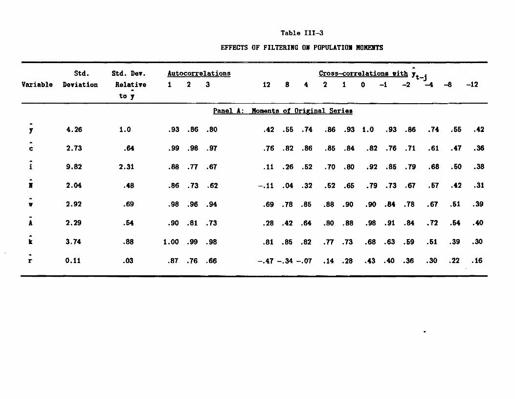
Table III-3

EFFECTS OF FILTERING ON POPULATIOI ROKEITS

Variable Std.

DeyiatioD Std. Dey. Relatiye

to 1

1utocorrelations 1 2 3 12 8 4

.. Cross-correlatioDB vith ' t -j

2 1 0 -1 -2 -4 -8 -12

Panel 1: Moments of Original Seriel

1 4.26 1.0 .93 .86 .80 .42 .55 .74 .86 .93 1.0 .93 .86 .74 .55 .42

c .. i

2.73

9.82

.64

2.31

.99

.88

.98

.77

.97

.67

.76

.11

.82

.26

.86

.52

.85

.70

.84

.80

.82

.92

.76

.85

.71

.79

.61

.68

.47

.50

.36

.38 .. I 2.04 .48 .86 .73 .62 -.11 .04 .32 .52 .65 .79 .73 .67 .57 .42 .31

v 2.92 .69 .98 .96 .94 .69 .78 .85 .88 .90 .90 .84 .78 .67 .51 .39 .. 1 2.29 .54 .90 .81 .73 .28 .42 .64 .80 .88 .98 .91 .84 .72 .54 .40 .. t 3.74 .88 1.00 .99 .98 .81 .86 .82 .77 .73 .68 .63 .59 .51 .39 .30

r 0.11 .03 .87 .76 .66 -.47 -.34 -.07 .14 .28 .43 .40 .36 .30 .22 .16

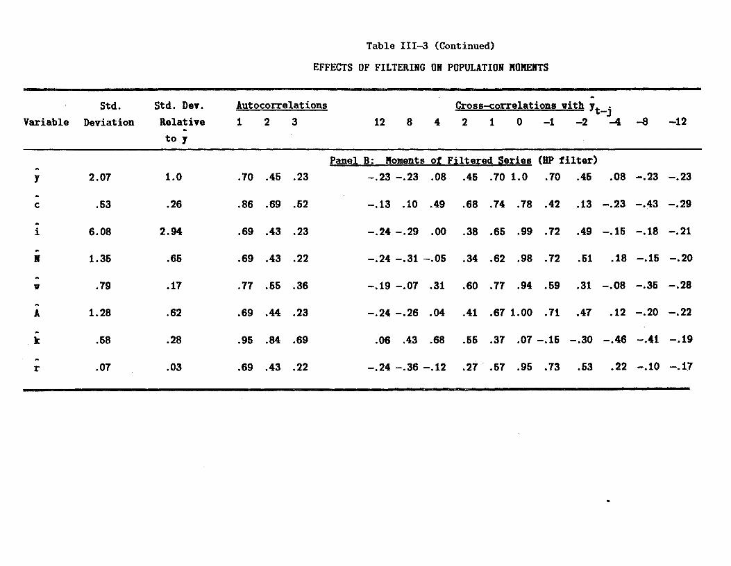
Table 111-3 (Continued)

EFFECTS OF FILTERING ON POPULATION MOKERTS

Variable Std.

DeTiation

Std. DeT. RelatiTe

to J

Autocorrelations

1 2 3 12 8 4

A

Cross-correlations vith J t .-J

2 1 0 -1 -2 -4 -8 -12

Panel B: Moments of Filtered aeries (BP filter)

J 2.07 1.0 .70 .45 .23 -.23 -.23 .08 .45 .70 1.0 .70 .45 .08 -.23 -.23

c .53 .26 .86 .69 .52 -.13 .10 .49 .68 .74 .78 .42 .13 -.23 -.43 -.29

A

i 6.08 2.94 .69 .43 .23 -.24 -.29 .00 .38 .66 .99 .72 .49 -.15 -.18 -.21 A

I 1.36 .66 .69 .43 .22 -.24 -.31 -.05 .34 .62 .98 .72 .51 .18 -.15 -.20

v .79 .17 .77 .55 .36 -.19 -.07 .31 .60 .77 .94 .69 .31 -.08 -.35 -.28

A

A 1.28 .62 .69 .44 .23 -.24 -.26 .04 .41 .67 1.00 .71 .47 .12 -.20 -.22

.. k .68 .28 .95 .84 .69 .06 .43 .68 .55 .37 .07 -.15 -.30 -.46 -.41 -.19

r .07 .03 .69 .43 .22 -.24 -.36 -.12 .27 ..57 .96 .73 .53 .22 -.10 -.17

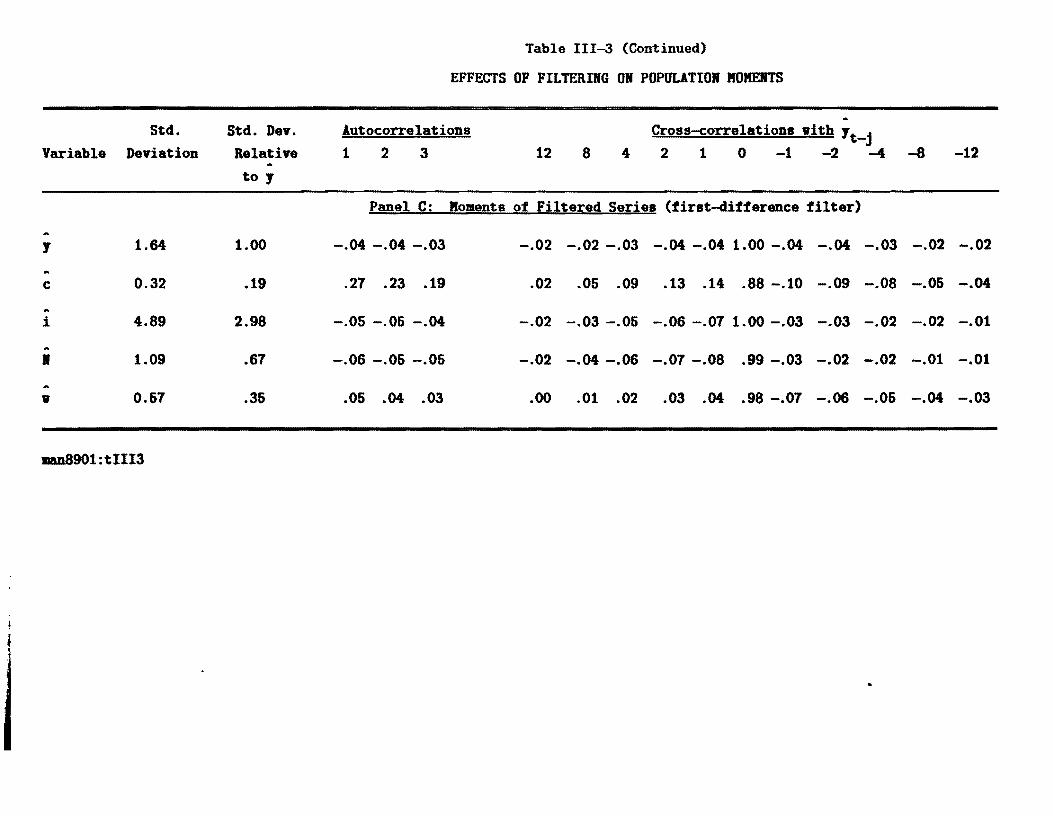
Table 111-3 (Continued)

EFFECTS OF FILTERING ON POPULATION MOKENTS

Variable Std.

Deviation Std. Dey. Relatiye

A

to J

Autocorrelations 1 2 3 12 8 4

A

Cross-correlationa with Jt-j 2 1 0 -1 -2 -4 -8 -12

Panel ~Mo.~nts Qf £iltered Series (tirat-ditterence tilter)

J 1.64 1.00 -.04 -.04 -.03 -.02 -.02 -.03 -.04 -.04 1.00 -.04 -.04 -.03 -.02 -.02

c 0.32 .19 .27 .23 .19 .02 .05 .09 .13 .14 .88 -.10 -.09 -.08 -.06 -.04

A

i 4.89 2.98 -.05 -.05 -.04 -.02 -.03 -.05 -.06 -.07 1.00 -.03 -.03 -.02 -.02 -.01

A

I 1.09 .67 -.06 -.06 -.05 -.02 -.04 -.06 -.07 -.08 .99 -.03 -.02 -.02 -.01 -.01

w 0.67 .36 .05 .04 .03 .00 .01 .02 .03 .04 .98 -.07 -.06 -.06 -.04 -.03

-.n8901 :tIII3

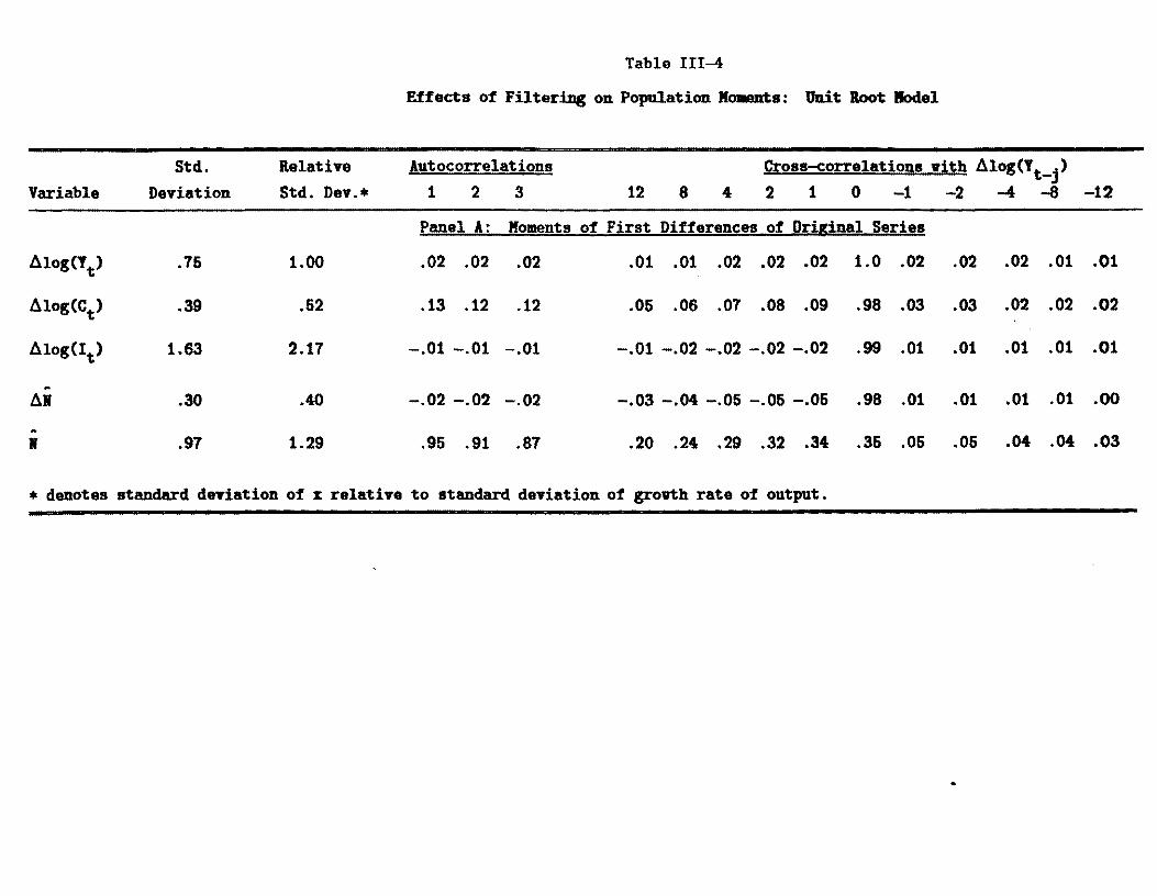
Table III-4

Effects of Filtering on Population lIo.ents: Unit Root Iodel

Std. Relatiye Autocorrelations Cross-correlations with ~log(Yt_j) Variable Deyiation Std. Dey.• 1 2 3 12 8 4 2 1 0 -1 -2 -4 -8 -12

Panel A: Moments of First Differences of Original Series

~log(Yt) .76 1.00 .02 .02 .02 .01 .01 .02 .02 .02 1.0 .02 .02 .02 .01 .01

~log(Ct) .39 .52 .13 .12 .12 .05 .06 .07 .08 .09 .98 .03 .03 .02 .02 .02

~log(It) 1.63 2.17 -.01 -.01 -.01 -.01 -.02 -.02 -.02 -.02 .99 .01 .01 .01 .01 .01

A

~. .30 .40 -.02 -.02 -.02 -.03 -.04 -.05 -.06 -.06 .98 .01 .01 .01 .01 .00

A

• .97 1.29 .95 .91 .87 .20 .24 .29 .32 .34 .36 .06 .06 .04 .04 .03

• denotes standard deviation of x relative to standard deviation of growth rate of output.

I

Table 111-4 (Continued)

Effects of FilteriDg on Population lIolmllts: Unit Root lIodel

Variable Std.

Deviation Relative Std. Dev.•

Autocorrelations

1 2 3 12 8 4

Cross-correlations vith log(Yt _j )

2 1 0 -1 -2 -4 -8 -12

Panel B: Moments of Filtered Series (HP Filter)

Yt .99 1 .68 .47 .28 -.24 -.20 .13 .47 .68 1 .68 .47 .13 -.20

Ct .63 .63 .72 .63 .36 -.21 -.10 .26 .66 .73 .98 .63 .40 .04 -.29

It 2.16 2.16 .67 .46 .27 -.26 -.26 .06 .41 .64 .99 .70 .61 .18 -.16

.39 .40 .67 .46 .26 -.27 -.31 -.02 .36 .60 .98 .71 .63 .23 -.11

• denotes standard deviation of BP filtered x relative to standard deviation of filtered output.

JIIIlD8901 :tIII4

-

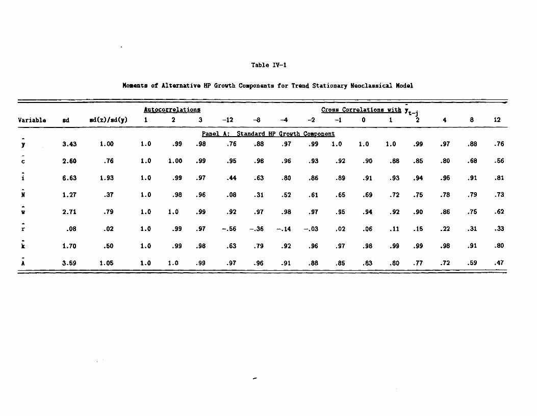
Table 1V-l

Mo.ants of Alternative HP Grovth Coaponents for Trend Stationary Neoclassical Model

. Autoco[[elations Qross Qorrelationg viti Jt-j

Variable ad ad(z)/ad(y) 1 2 3 -12 -a -4 -2 -1 0 1 2 4 8 12

fanel A: ~tandard HP growth QoaRonent

J 3.43 1.00 1.0 .99 .98 .76 .88 .97 .99 1.0 1.0 1.0 .99 .97 .88 .76

c 2.60 .76 1.0 1.00 .99 .95 .98 .96 .93 .92 .90 .88 .85 .80 .68 .56

· i 6.63 1.93 1.0 .99 .97 .44­ .63 .80 .86 .89 .91 .93 .94­ .95 .91 .81

· N 1.27 .37 1.0 .98 .96 .08 .31 .52 .61 .65 .69 .72 .75 .78 .79 .73

v 2.71 .79 1.0 1.0 .99 .92 .97 .98 .97 .95 .94 .92 .90 .86 .75 .62

r .08 .02 1.0 .99 .97 -.56 -.36 -.14 -.03 .02 .06 .11 .15 .22 .31 .33

· k 1.70 .50 1.0 .99 .98 .63 .79 .92 .96 .97 .98 .99 .99 .98 .91 .80

· A 3.69 1.05 1.0 1.0 .99 .97 .96 .91 .88 .85 .83 .80 .77 .72 .59 .47

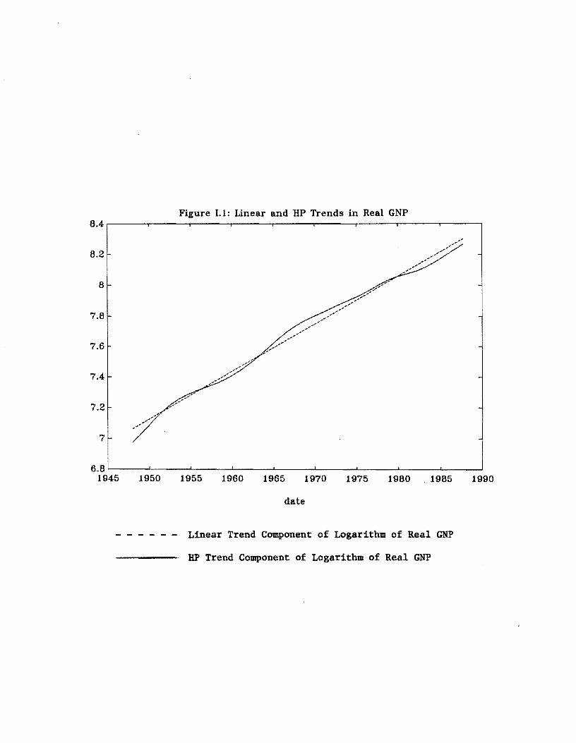
Figure 1.1: Linear and UP Trends in Real GNP 8.4~----~-----r----~------r-----'------.-----.~----~----~

8.2

8

7.8

7.6

7.4

7.2

7

6.8~----~----L-----~----~----~----~----~----~----~ 1945 1950 1955 1960 1965 1970 1975 1980 . 1985 1990

date

- - - - - - Linear Trend Component of Logarithm of Real GNP

HP Trend Component of Logarithm of Real GNP

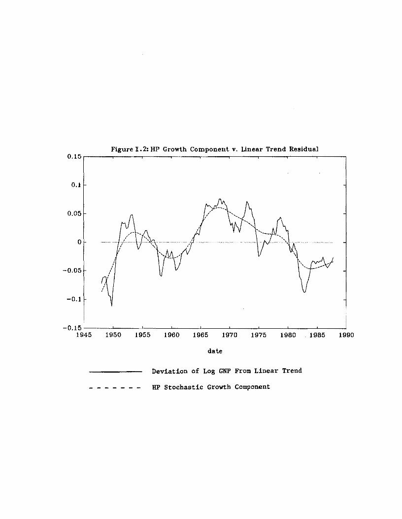
Figure 1.2: HP Growth Component v. Linear Trend Residual 0.15r-----~----~----_r----_.----_,------r_----~----~----~

0.1

0.05

o

-0.05

-0.1

-0.15~----~----~----~------~----~----~------~----~----~

1945 1950 1955 1960 1965 1970 1975 1980 1985 1990

date

Deviation of Log GNP From Linear Trend

- - - - - - - UP Stochastic Growth Component

-0.05

Figure L 3: HP Cyclical Component of Real GNP 0.15~----~----.-----~----~----~----~-----.-----.-----;

0.1

0.05

o

-0.1

-0.15~----~----~----~----~----~------L-----~----~____~ 1945 1950 1955 1960 1965 1970 1975 1980 . 1985 1990

date

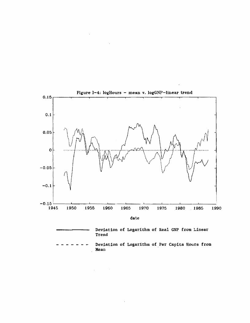
Figure 1-4: logHours - mean v. logGNP-linear trend 0.15._----~-----r----_,------~----~----_.----~._----~----~

0.1

1\ " \ \ \ \ \ \

0.05

I , I....,,

r,'''''/''\o ·······iJ~"'I'I/ioI··~·······l········H ........ , ... ,/ \ /'...

I ... I ...

I " , " \ l \\\.l"','Y \ ;­

~ \'J' \ I

\-0.05

-0.1

-0.15~----~----~----~------~----~----~------~----~----~ 1945 1950 1955 1960 1965 1970 1975 1980 1985 1990

date

Deviation of Logarithm of Real GNP from Linear Trend

Deviation of Logarithm of.Per Capita Hours from Mean

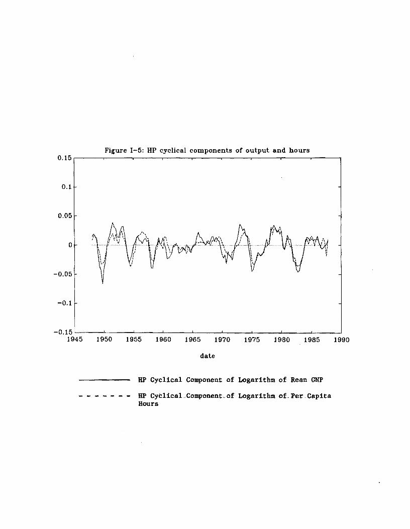
-0.05

-0.1

Figure 1-5: HP cyclical components of output and hours 0.15r-----~----_r----~------r_----~----_r----~------~----~

0.1

0.05

o

-0.15~----~----~----~------~----~-----L----~------L-----~ 1945 1950 1955 1960 1965 1970 1975 1980 1985 1990

date

- - - - - - -

HP Cyclical Component of L~garithm of Rean GNP

HP CyClical ..Component,of Logarithm of_ Per. Capita Hours

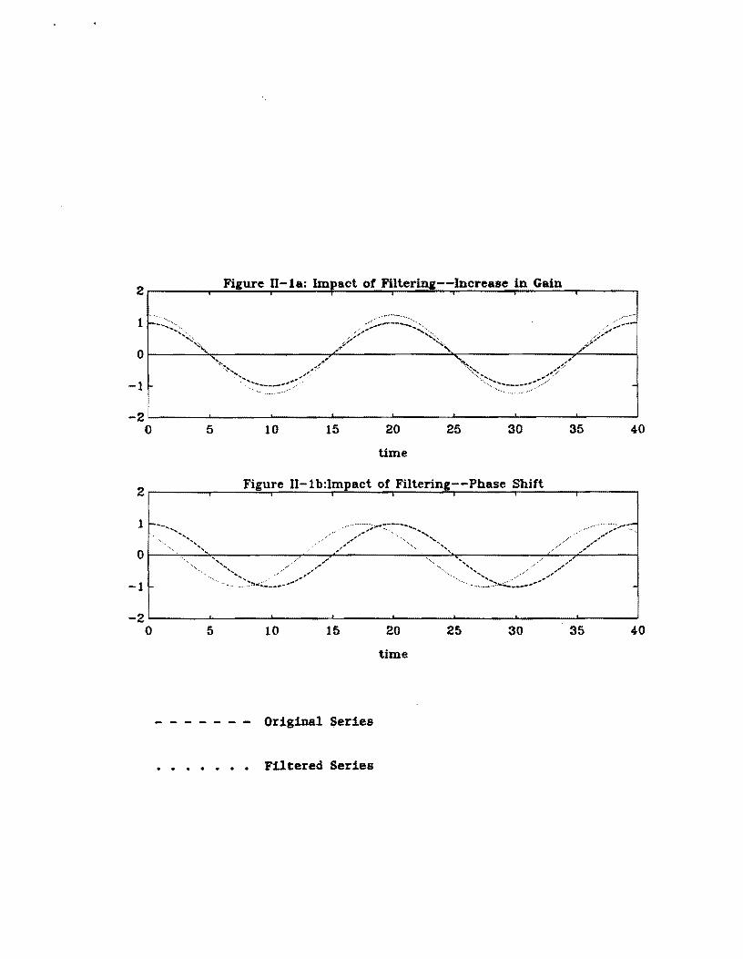
2r-______~F~i~g~u~r~e~n~-~1~a~:~bn~p~a~c~t~o~f~F~irlt~e~r~1n~ll~·-_-~ln~c~r~e~a~s~e~i~n~G~a~ln~~----~

,' .......'_...",

-2~----~------~----~------~------~----~------~----~ o 5 10 15 20 25 30 35 40

time

2r-____~-----F~ig~u~r-e--II---l-b~:I~m~p~a-c-t--o-f~F-il-t-e-ri_n~g~-_-_P_h_a_s_e~S_h_if_t____~____~

1 -'-... , ....'~...... ::;:;:~'::~,~--......." .' ".' '-:~':';;,-"~.~ , . "-'........ ,ii", /" , ..

Or---~-·,~,,~----------~--~,_/_'--------""-'~-'-"~'~----------~'_/-T~/-/----~ """" ...., ..."" / ,,,,,,,,,,,

.. >~~><:~:~--",/-1

-2~----~------~------~------~----~------~------~----~ o 5 10 15 20 25 30 35 40

time

- - - - - - - Original Series

. . . . . . . Filtered Series

, .

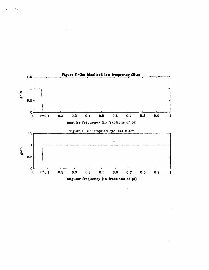
;'Aa\oU .. D-2a: idealized low frequency filter 1.5~----~----~~--~~--~~~~~~~~--~~--~.~----~----,

1-1 I

I• I I0.5 -•I

I I••I O~__~i'~____~____~~____~____~____~____~____~__________~

o w*O.l 0.2 0.3 0.4 0.5 0.6 0.7 0.8 0.9

ancular frequency (in fractions of pi)

I:-I'll IIID

1

0.5

r-----------------':: I

f I I:,:

O~~~-------~-----~-------~------~-----L----~~---~------~----~ o w*O.l 0.2 0.3 0.4 0.5 0.6 0.7 0.8 0.9 1

ancular frequency (in fractions of pi)

1

, ..•

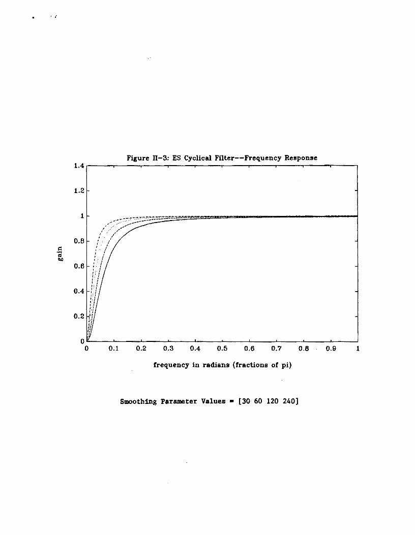
Figure II-3: ES Cyclical Filter--Frequency Response 1.4

1.2

1 ,

-', I

I I

0.8 i

s::.... CIS IiIli

0.6

0.4

0.2

0.5 0.6 0.7 0.8 0.9 1

frequency in radians (fractions of pi)

Smoothing Parameter Values • [30 60 120 240]

."

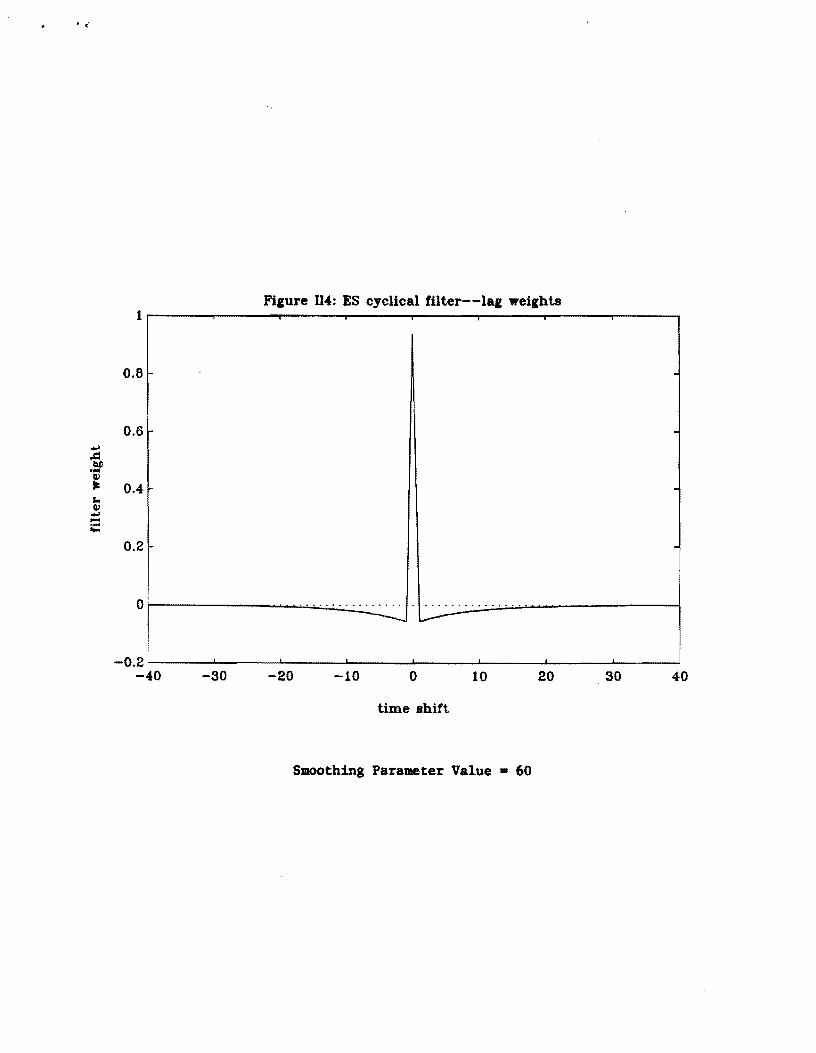
Fi,ure n4: ES cyclical fUter--la, wei,hts 1~----~------~-------r------~------~------r-----~r------,

0.8

.0.6.. .c: ....~ Q)

It 0.4 -... Q)

.... ..-.... 0.2

or------....................:...:. ..:...:....~....... .L..--'" -,.:'',;..;.''..:..;.'.:..:,...:.,:..'.:,..:.'.............................-----"'1.. ..:....;..',.:..:'....:...: ___

-0.2~----~------~------~----~------~------~----~~----~ -40 -30 -20 -10 o 10 20 30 40

time shift

Smoothing Parameter Value • 60

.,' /

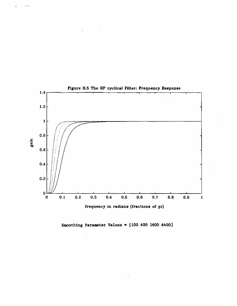
I j

I i i,, ! I

i, i i i,, i i i i•i i i I I i I

, ,

o~~--~----~----~----~----~----~----~----~----~----~ o 0.1 0.2 0.3 0.4 0.5 0.6 0.7 0.8 OJ} 1

frequency in radians (fractions of pi)

Smoothing Parameter Values - [100 400 1600 6400]

1.4­

1.2

1

0.8 C.... aI ~

0.6

0.4­

0.2

Figure JI.5 The HP cyclical Filter: Frequency Response

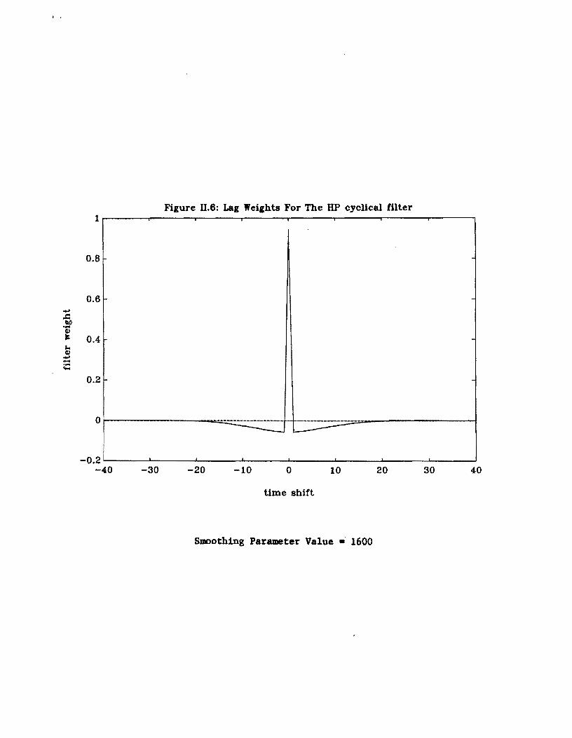
I _

Figure U.6: Lag Weights For The HP cyclical filter 1r------r------~----~------~----~------~----~~----,

0.8

0.6 ., ,Q ~... G,)

at 0.4 G,).,"'" .... -....

0.2

o1""----------..::.:--:;::--:::---------------- - -------------..::--::;--=--,...---------1 ~~

-0.2~----~------~----~------~----~------~----~~----~ -40 -30 -20 -10 o 10 20 30 40

time shift

Smoothing Parameter Value - 1600

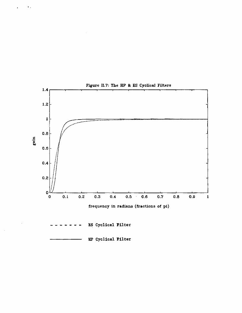
I,

Filure 11.7: The HP & ES Cyclical Filters 1.4~--~----~-----r----~----T-----r---~~--~----~----,

1.2

1 ..~ ...""-....---...----......------------... ­,-II'

,/'O.B r­

/ " ....= ct! ~

!I .0.6 ,

I

I ,I , I

0.4 J I,,, !,

0.2

)J o 0.1 0.2 0.3 0.4 0.5 0.6 0.7 O.B 0.9

frequency in radians (fractions of pi)

- - - - - - - ES Cyclical Filter

UP Cyclical Filter

1

-------

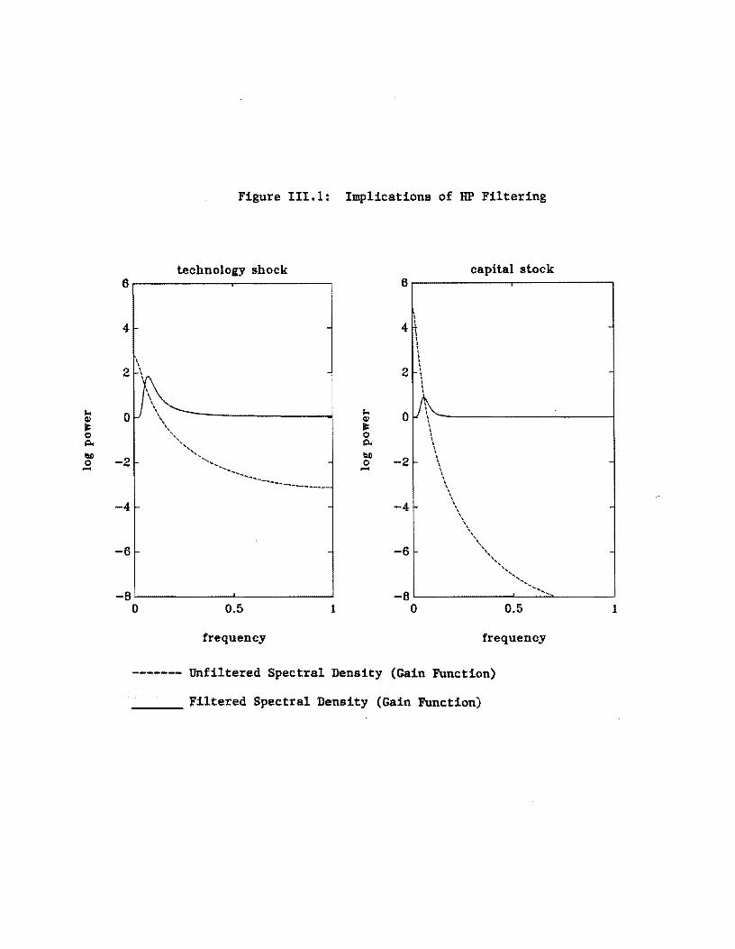
Figure 111.1: Implications of HP Filtering

technology shock capital stock 6

4

-4

-6

-B~----------~----------~ o 0.5 1

frequency

6~----------~----------~

4~

2

I I I I I I

\\

~------------------------~o \ \ \ \ I I I \ \

-2 \

\ \ \ \ \ \ \ \

-4 \

\ \ \ \

\"\

-6 "~"~'ll"~ "

' ............ -B~----------~~--',~,L-------~

o 0.5 1

frequency

------- Unfiltered Spectral Density (Gain Function)

Filtered Spectral Density (Gain Function)

Rochester Center for Economic Research University of Rochester Department of Economics

Rochester, NY 14627

1988-1989 DISCUSSION PAPERS

WP#118 ADVERSE SELECTION, AGGREGATE UNCERTAINTY, AND THE ROLE FOR MUTUAL INSURANCE COMPANIES by Bruce D. Smith and Michael J. Stutzer, February 1988

WP#119 INTEREST ON RESERVES AND SUNSPOT EQUILIBRIA: RECONSIDERED by Bruce D. Smith, February 1988

FRIEDMAN'S PROPOSAL

WP#120 INTERNATIONAL FINANCIAL INTERMEDIATION AND AGGREGATE FLUCTUATIONS UNDER ALTERNATIVE EXCHANGE RATE REGIMES by Jeremy Greenwood and Stephen D. Williamson, February 1988

WP#121 FINANCIAL DEREGULATION, MONETARY POLICY, AND CENTRAL BANKING by Marvin Goodfriend and Robert G. King, February 1988

WP#122 BANK RUNS IN OPEN ECONOMIES AND THE INTERNATIONAL TRANSMISSION OF PANICS by Peter M. Garber and Vittorio U. Grilli, March 1988

WP#123 CAPITAL ACCUMULATION IN THE THEORY OF LONG RUN GROWTH by Paul M. Romer, March 1988

WP#124 FINANCIAL INTERMEDIATION AND ENDOGENOUS GROWTH by Valerie R.Bencivenga and Bruce D.Smith, March 1988

WP#125 UNEMPLOYMENT, THE VARIABILITY OF HOURS, AND THE PERSISTENCE OF "DISTURBANCES": A PRIVATE INFORMATION APPROACH by Bruce D. Smith, March 1988

WP#126 WHAT CAN BE DONE WITH BAD SCHOOL PERFORMANCE DATA? by Eric Hanushek and Lori Taylor, March 1988

WP#127 EQUILIBRIUM MARKETING STRATEGIES: IS THERE ADVERTISING~ IN TRUTH? by Ignatius Horstmann and Glenn MacDonald, revised, March 1988

WP#128 REAL EXCHANGE RATE VARIABILITY UNDER PEGGED AND FLOATING NOMINAL EXCHANGE RATE SYSTEMS: AN EQUILIBRIUM THEORY by Alan C. Stockman, April 1988

WP#129 POST-SAMPLE PREDICTION TESTS FOR GENERALIZED METHOD OF MOMENT ESTIMATORS by Dennis Hoffman and Adrian Pagan', April 1988

WP#130 GOVERNMENT SPENDING IN A SIMPLE MODEL OF ENDOGENOUS GROWTH by Robert J. Barro, May 1988

2

WP#131 FINANCIAL DEVELOPMENT, GROWTH, AND THE DISTRIBUTION OF by Jeremy Greenwood and Boyan Jovanovic, May 1988

INCOME

WP#132 EMPLOYMENT AND HOURS OVER THE BUSINESS CYCLE by Jang-ok Cho and Thomas F. Cooley, May 1988

WP#133 A REFINEMENT AND EXTENSION OF THE NO-ENVY CONCEPT by Dimitrios Diamantaras and William Thomson, May 1988

WP#134

WP#135

NASH SOLUTION AND UNCERTAIN DISAGREEMENT POINTS by Youngsub Chun and William Thomson, May 1988 . NON-PARAMETRIC ESTIMATION AND THE RISK PREMIUM by Adrian Pagan and Y. Hong, May 1988

WP#136 CHARACTERIZING THE NASH BARGAINING SOLUTION WITHOUT PARETO-OPTIMALITY by Terje Lensberg and William Thomson, May 1988

WP#137 SOME SIMULATION STUDIES OF NON-PARAMETRIC ESTIMATORS by Y. Hong and A. Pagan, June 1988

WP#138 SELF-FULFILLING EXPECTATIONS, SPECULATIVE ATTACKS AND CAPITAL CONTROLS by Harris Dellas and Alan C. Stockman, June 1988

WP#139 APPROXIMATING SUBOPTIMAL DYNAMIC EQUILIBRIA: APPROACH by Marianne Baxter, June 1988

AN EULER EQUATION

WP#140 .BUSINESS.CYCLES AND ,THE EXCHANGE· RATE SYSTEM: SOME INTERNATIONAL EVIDENCE by Marianne Baxter and Alan C. Stockman, June 1988

WP#141 RENT SHARING IN AN EQUILIBRIUM MODEL OF MATCHING AND TURNOVER by Kenneth J. McLaughlin, June 1988

WP#142 CO-MOVEMENTS IN RELATIVE COMMODITY PRICES AND FLOWS: A SIMPLE MODEL by Ronald W. Jones, July 1988

INTERNATIONAL CAPITAL

WP#143 WAGE §ENSITIVITY RANKINGS AND TEMPORAL CONVERGENCE by Ronald W. Jones and Peter Neary, July 1988

WP#144 FOREIGN MONOPOLY AND OPTIMAL TARIFFS FOR THE SMALL OPEN ECONOMY by Ronald W. Jones and Shumpei Takemori, July 1988

WP#145 THE ROLE OF SERVICES IN PRODUCTION AND INTERNATIONAL TRADE: THEORETICAL FRAMEWORK by Ronald W. Jones and Henryk Kierzkowski, July 1988

A

WP#146 APPRAISING THE OPTIONS FOR INTERNATIONAL TRADE IN SERVICES by Ronald W. Jones and Frances Ruane, July 1988

3

WP#147 SIMPLE METHODS OF ESTIMATION AND INFERENCE FOR SYSTEMS CHARACTERIZED BY DETERMINISTIC CHAOS by Mahmoud El-Gamal, August 1988

WP#148 THE RICARDIAN APPROACH TO BUDGET DEFICITS by Robert J. Barro, August 1988

WP#149 A MODEL OF NOMINAL CONTRACTS by Bruce D. Smith, August 1988

WP#150 A BUSINESS CYCLE MODEL WITH PRIVATE INFORMATION by Bruce D. Smith, August 1988

WP#151 ASYMPTOTIC LIKELIHOOD BASED PREDICTION FUNCTIONS by Thomas F. Cooley, August 1988

WP#152 MORAL HAZARD. IMPERFECT RISK-SHARING, AND THE BEHAVIOR OF ASSET RETURNS by James A. Kahn, August 1988

WP#153 SPECIALIZATION. TRANSACTIONS TECHNOLOGIES, AND MONEY GROWTH by Harold Cole and Alan C. Stockman, August 1988

WP#154 SAVINGS. INVESTMENT AND INTERNATIONAL CAPITAL FLOWS by Linda L. Tesar. August 1988

WP#155 THE INFLATION TAX IN A REAL BUSINESS CYCLE MODEL by Thomas F. Cooley and Gary D. Hansen. August 1988

WP#156 RAW MATERIALS. PROCESSING ACTIVITIES AND PROTECTIONISM by Ronald W. Jones ,and Barbara J . Spencer., September 1988

WP#157 A TEST OF THE HARRIS ERGODICITY OF STATIONARY DYNAMICAL ECONOMIC MODELS by Ian Domowitz and Mahmoud EI-Gamal, September 1988

WP#158 SYMMETRIC STOCHASTIC GAMES OF RESOURCE EXTRACTION: THE EXISTENCE OF NON-RANDOMIZED STATIONARY EQUILIBRIUM by Mukul Majumdar and Rangarajan Sundaram, September 1988

WP#159 SOME CONSEQUENCES OF CREDIT RATIONING IN AN ENDOGENOUS GROWTH MODEL by Valerie Bencivenga and Bruce Smith, September 1988

WP#160 COMPETITIVE DIFFUSION by Boyan Jovanovic and Glenn MacDonald. September 1988

WP#161 EXCHANGE RATES, THE CURRENT ACCOUNT, AND MONETARY POLICY by Alan C. Stockman, October 1988

WP#162 DIAGNOSTIC TESTS FOR MODELS BASED ON INDIVIDUAL DATA: A SURVEY by Adrian Pagan and Frank Vella, October 1988

4

WP#163 EFFICIENCY BOUND CALCULATIONS FOR A TIME SERIES MODEL WITH CONDITIONAL HETEROSKEDASTICITY by John Heaton and Masao Ogaki, November 1988

WP#164 TAX ANALYSIS IN A DYNAMIC STOCHASTIC MODEL ON MEASURING HARBERGER TRIANGLES AND OKUN GAPS by Jeremy Greenwood and Gregory W. Huffman, November 1988

WP#165 THE POSITIVE ECONOMICS OF METHODOLOGY by James A. Kahn, Steven E. Landsburg, and Alan C. Stockman, . November 1988

WP#166 MULTIPLIERS IN EQUILIBRIUM BUSINESS CYCLE MODELS by Marianne Baxter and Robert G. King, November 1988

WP#167 DYNAMIC REAL TRADE MODELS: NEW DIRECTIONS FOR OPEN ECONOMY MACROECONOMICS by Marianne Baxter, December 1988

WP#168 WHY IS PRODUCTION MORE VOLATILE THAN SALES? THEORY AND EVIDENCE ON THE STOCKOUT-AVOIDANCE MOTIVE FOR INVENTORY-HOLDING by James A. Kahn, December 1988

WP#169 BUSINESS CYCLES. STYLIZED FACTS, AND THE EXCHANGE RATE REGIME: EVIDENCE FROM THE UNITED STATES by Marianne Baxter, December 1988

WP#170 THE INDIRECT AND DIRECT SUBSTITUTION EFFECTS by Masao Ogaki, December 1988

WP#171 RATIONAL ·RESPONSETOUNPRECEDENTED>POLICIES: THE 1979 CHANGE IN,. FEDERAL RESERVE OPERATING PROCEDURES by Marianne Baxter. January 1989

WP#172 THE TRAGEDY OF THE COMMONS? A CHARACTERIZATION OF STATIONARY PERFECT EQUILIBRIUM IN DYNAMIC GAMES by Prajit K. Dutta and Rangarajan K. Sundaram, January 1989

WP#173 EXTERNALITIES AND ASYMMETRIC INFORMATION by Jeremy Greenwood and R. Preston McAfee, January 1989

WP#174 TESTING FOR CONTRACTING EFFECTS ON EMPLOYMENT by Mark Bils. January 1989

WP#175 CREDIBLE BORROWING CONSTRAINTS WITH RENEGOTIABLE DEBT by James A. Kahn. February 1989

WP#176 REAL EXPECTATIONS: A HARMONY THEORETIC APPROACH TO DECISION MAKING UNDER UNCERTAINTY by Mahmoud A. El-Gamal, February 1989

WP#177 COOPERATIVE MODELS OF BARGAINING by William Thomson. February 1989

5

WP#178 NO-ENVY, CONSISTENCY AND MONOTONICITY IN ECONOMIES WITH INDIVISIBILITIES by Koichi Tadenuma and William Thomson, March 1989

-WP#179 OUTPUT GROWTH, THE REAL WAGE, AND EMPLOYMENT FLUCTUATIONS by Zvi Hercowitz and Michael Sampson, March 1989

WP#180 MIGRATION BETWEEN HOME COUNTRY AND DIASPORA: by Zvi Hercowitz and David Pines, March 1989

AN ECONOMIC ANALYSIS

WP#181 NONPARAMETRIC HAZARD ESTIMATION WITH TIME VARYING DISCRETE COVARIATES by Siu Fai Leung and Wing Hung Wong, March 1989

WP#182 NEW PREDICTIONS FROM THE ECONOMICS OF UNIONISM by Glenn M. MacDonald and Christopher Robinson, March 1989

WP#183 REPEATED GAMES, FINITE AUTOMATA, AND COMPLEXITY by Jeffrey S. Banks and Rangarajan K. Sundaram, April 1989

WP#184 INTERTEMPORAL SUBSTITUTION AND A-GONSTANT COMPARATIVE STATICS by Kenneth J. McLaughlin, April 1989

WP#185 THE STOCK MARKET AND INVESTMENT by Robert J. Barro, May 1989

WP#186 GOVERNMENT SPENDING IN A SIMPLE MODEL OF ENDOGENOUS by Robert J. Barro, May 1989

GROWTH

WP#187 NEW CLASSICALS AND KEYNESIANS, by Robert J. Barro, May 1989

OR THE GOOD GUYS AND THE BAD GUYS

WP#188 THE CYCLICAL BEHAVIOR OF PRICES by Thomas F. Cooley and Lee E. Ohanian, May 1989

WP#189 BARGAINING PROBLEMS WITH CLAIMS by Youngsub Chun and William Thomson, June 1989

WP#190 ENTRY AND EXIT IN PERFECT COMPETITION: PART I: THEORY by Boyan Jovanovic and Glenn M. MacDonald, June 1989

WP#191 MARKET EQUILIBRIA WITH NOT-FOR-PROFIT FIRMS by Charles E. Phelps and Itai Sened, June 1989

WP#192 THE CONSISTENCY PRINCIPLE by William Thomson, August 1989

WP#193 TRANSVERSALITY CONDITION AND OPTIMALITY IN A CLASS OF HORIZON CONTINUOUS TIME ECONOMIC MODELS by Siu Fai Leung, August 1989

INFINITE

WP#194 VERTICAL FORECLOSURE AND INTERNATIONAL TRADE POLICY by Barbara J. Spencer and Ronald W. Jones, August 1989

6

WP#195 TRADE AND PROTECTION IN VERTICALLY RELATED MARKETS by Barbara J. Spencer and Ronald W. Jones, August 1989

WP#196 COMMUNICATION AND EFFICIENCY IN COORDINATION GAMES by Jeffrey S. Banks and Randall L. Calvert, August 1989

WP#197 FULL INSURANCE IN THE PRESENCE OF AGGREGATE UNCERTAINTY by Barbara J. Mace, August 1989

WP#198 UNDERSTANDING REAL BUSINESS CYCLES by Charles I. Plosser, August 1989

WP#199 A SIMPLE ESTIMATOR FOR SIMULTANEOUS MODELS WITH CENSORED ENDOGENOUS REGRESSORS by Frank Vella, August 1989

WP#200 DYNAMIC INEFFICIENCY IN AN ECONOMY WITH LAND by Changyong Rhee, August 1989

WP#201 ECONOMIC GROWTH IN A CROSS SECTION OF COUNTRIES by Robert J. Barro, September 1989

WP#202 ADVERSE SELECTION IN THE OVERLAPPING GENERATIONS MODEL by Costas Azariadis and Bruce D. Smith, October 1989

WP#203 MULTIPLE AND SUNSPOT EQUILIBRIA UNDER INTEREST RATE AND MONEY SUPPLY RULES by Bruce D. Smith. October 1989

WP#204 REAL BUSINESS CYCLES AND THE TEST OF THE ADELMANS by Robert G. King and ,Charles I.Plosser. October 1989

WP#205 LOW FREQUENCY FILTERING AND REAL BUSINESS CYCLES by Robert G. King and Sergio T. Rebelo. October 1989

WP#206 TRANSITIONAL DYNAMICS AND ECONOMIC GROWTH IN THE NEOCLASSICAL MODEL by Robert G. King and Sergio T. Rebelo, November 1989