RM Bridge Professional Engineering Software for Bridges of all Types RM Bridge V8i October 2010 TRAINING PRESTRESSING BASIC - RM - PART2: EC

Welcome message from author
This document is posted to help you gain knowledge. Please leave a comment to let me know what you think about it! Share it to your friends and learn new things together.
Transcript

RM Bridge Professional Engineering Software for Bridges of all Types
RM Bridge V8i
October 2010
TRAINING PRESTRESSING BASIC - RM -
PART2: EC
RM Bridge
Training Prestressing Basic - RM - Part2: EC I
© Bentley Systems Austria
Contents
1 General ................................................................................................................... 1-1
1.1 Design Codes ................................................................................................. 1-1
1.2 Actions ........................................................................................................... 1-1
1.2.1 Permanent actions and Creep & Shrinkage ............................................... 1-1
1.2.2 Traffic loads ............................................................................................... 1-1
1.2.3 Wind loads ................................................................................................. 1-7
1.2.4 Temperature load ....................................................................................... 1-9
1.2.5 Settlements ............................................................................................... 1-10
1.3 Combinations ............................................................................................... 1-11
1.4 Design checks .............................................................................................. 1-12
1.4.1 Servicebility limit state ............................................................................ 1-12
1.4.2 Ultimate limit state ................................................................................... 1-13
2 Lesson 13: Definition of Additional Loads ......................................................... 2-14
2.1 Definition of Settlement Load Cases ........................................................... 2-14
2.2 Definition of Temperature Load Cases ........................................................ 2-15
2.3 Definition of Wind Forces ........................................................................... 2-17
2.4 Definition of Braking Forces ....................................................................... 2-19
3 Lesson 14: Calculation and Superposition of additional loads ............................ 3-20
3.1 Calculation and superposition of Settlement loads ...................................... 3-20
3.2 Calculation and superposition of temperature loads .................................... 3-23
3.3 Calculation and superposition of wind loads ............................................... 3-24
3.4 Calculation and superposition of braking loads ........................................... 3-25
4 Lesson 15: Traffic Loads ..................................................................................... 4-26
4.1 Definition of Traffic Lanes .......................................................................... 4-27
4.2 Definition of Load Trains ............................................................................ 4-29
4.3 Traffic Calculation ....................................................................................... 4-31
4.3.1 Calculation of influence lines .................................................................. 4-31
4.3.2 Calculation and superposition of the tandem system ............................... 4-32
RM Bridge
Training Prestressing Basic - RM - Part2: EC II
© Bentley Systems Austria
4.3.3 Calculation and superposition of the UDL loads ..................................... 4-34
4.3.4 Calculation and superposition of the Fatigue load models ...................... 4-35
5 Lesson 16: Load Combinations ........................................................................... 5-36
5.1 Definition of the Load Combination ............................................................ 5-36
5.2 Calculation of the load combinations .......................................................... 5-39
6 Lesson 17: Fibre Stress Check ............................................................................. 6-40
7 Reinforced concrete checks – General ................................................................. 7-42
8 Lesson 18: Crack Check ...................................................................................... 8-44
9 Lesson 19: Ultimate Load Capacity Check ......................................................... 9-46
10 Lesson 20: Shear Capacity Check ..................................................................... 10-48
11 Lesson 22: Fatigue Check .................................................................................. 11-49
12 Lesson 23: Lists and Plots ................................................................................. 12-50
Training Prestressing Basic - RM - Part2: EC 1-1
© Bentley Systems Austria
1 General
1.1 Design Codes
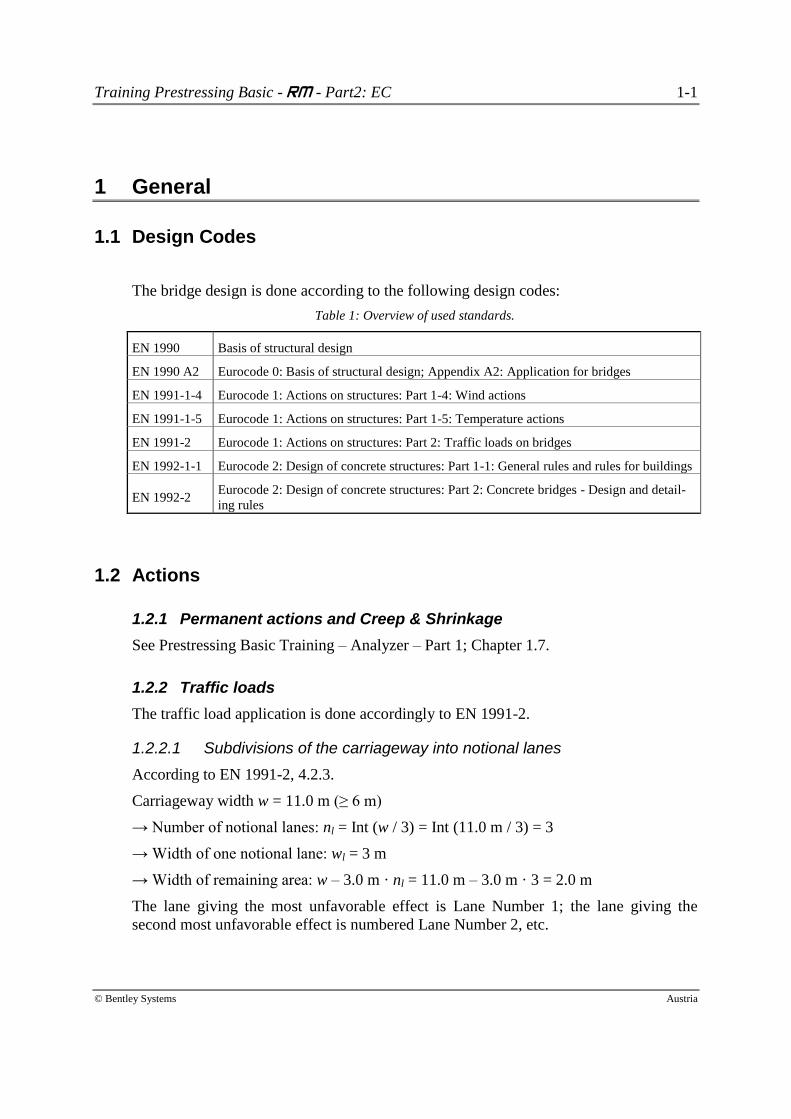
The bridge design is done according to the following design codes:
Table 1: Overview of used standards.
EN 1990 Basis of structural design
EN 1990 A2 Eurocode 0: Basis of structural design; Appendix A2: Application for bridges
EN 1991-1-4 Eurocode 1: Actions on structures: Part 1-4: Wind actions
EN 1991-1-5 Eurocode 1: Actions on structures: Part 1-5: Temperature actions
EN 1991-2 Eurocode 1: Actions on structures: Part 2: Traffic loads on bridges
EN 1992-1-1 Eurocode 2: Design of concrete structures: Part 1-1: General rules and rules for buildings
EN 1992-2 Eurocode 2: Design of concrete structures: Part 2: Concrete bridges - Design and detail-
ing rules
1.2 Actions
1.2.1 Permanent actions and Creep & Shrinkage
See Prestressing Basic Training – Analyzer – Part 1; Chapter 1.7.
1.2.2 Traffic loads
The traffic load application is done accordingly to EN 1991-2.
1.2.2.1 Subdivisions of the carriageway into notional lanes
According to EN 1991-2, 4.2.3.
Carriageway width w = 11.0 m (≥ 6 m)
→ Number of notional lanes: nl = Int (w / 3) = Int (11.0 m / 3) = 3
→ Width of one notional lane: wl = 3 m
→ Width of remaining area: w – 3.0 m · nl = 11.0 m – 3.0 m · 3 = 2.0 m
The lane giving the most unfavorable effect is Lane Number 1; the lane giving the
second most unfavorable effect is numbered Lane Number 2, etc.
Training Prestressing Basic - RM - Part2: EC 1-2
© Bentley Systems Austria
1.2
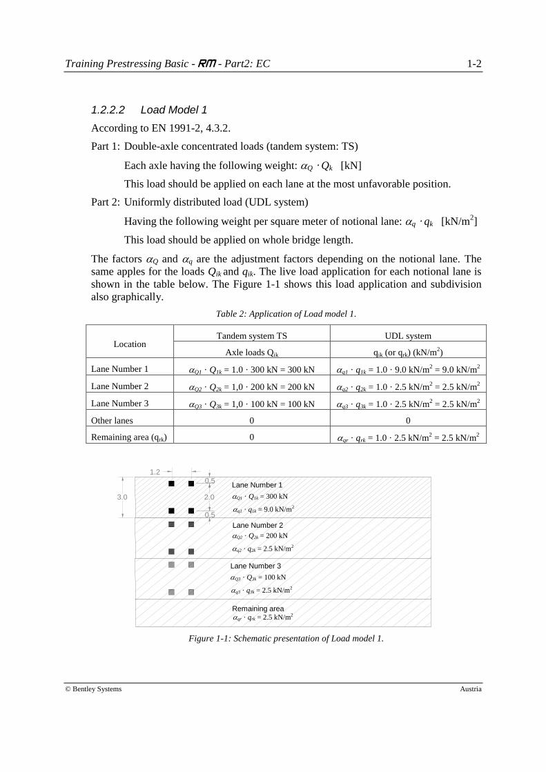
1.2.2.2 Load Model 1
According to EN 1991-2, 4.3.2.
Part 1: Double-axle concentrated loads (tandem system: TS)
Each axle having the following weight: Q Qk [kN]
This load should be applied on each lane at the most unfavorable position.
Part 2: Uniformly distributed load (UDL system)
Having the following weight per square meter of notional lane: q qk [kN/m2]
This load should be applied on whole bridge length.
The factors Q and q are the adjustment factors depending on the notional lane. The
same apples for the loads Qik and qik. The live load application for each notional lane is
shown in the table below. The Figure 1-1 shows this load application and subdivision
also graphically.
Table 2: Application of Load model 1.
Location Tandem system TS UDL system
Axle loads Qik qik (or qrk) (kN/m2)
Lane Number 1 Q1 · Q1k = 1.0 · 300 kN = 300 kN q1 · q1k = 1.0 · 9.0 kN/m2 = 9.0 kN/m
2
Lane Number 2 Q2 · Q2k = 1,0 · 200 kN = 200 kN q2 · q2k = 1.0 · 2.5 kN/m2 = 2.5 kN/m
2
Lane Number 3 Q3 · Q3k = 1,0 · 100 kN = 100 kN q3 · q3k = 1.0 · 2.5 kN/m2 = 2.5 kN/m
2
Other lanes 0 0
Remaining area (qrk) 0 qr · qrk = 1.0 · 2.5 kN/m2 = 2.5 kN/m
2
Figure 1-1: Schematic presentation of Load model 1.
0.5
2.0
0.5
3.0
Lane Number 3
Lane Number 2
Lane Number 1
q1 · q1k = 9.0 kN/m2
Q1 · Q1k = 300 kN
Q2 · Q2k = 200 kN
q2 · q2k = 2.5 kN/m2
q3 · q3k = 2.5 kN/m2
Q3 · Q3k = 100 kN
Remaining area
qr · qrk = 2.5 kN/m2

Training Prestressing Basic - RM - Part2: EC 1-3
© Bentley Systems Austria
1.2.2.3 Preparation of Traffic Lanes and Trains for the calculation
The wheel loads of the tandem system can be simplified into two axial loads for the
calculation on a global one-beam system. The same applies for the UDL load, in which
the load is simplified to a uniformly distributed load.
To simplify the input the following principle will be used. The UDL load will be ap-
plied over the whole carriageway width by two traffic lanes (one on each side) and one
load train with constant load of 2.5 kN/m2. The difference to the Lane number 1 (9.0
kN/m2) will be applied with an additional load train (9.0 – 2.5 = 6.5 kN/m
2) on both
outer sides of the carriageway (see Figure 1-1). For the longitudinal bending moment
and shear force the subdivision in the transversal direction is irrelevant. However, the
maximum and minimum torsion moments are covered within this subdivision.
Same applies for the positioning of the different TS Loads. They have to be positioned
only at the outermost edges (left and right) of the carriageway.
The combination of the different TS loads and different UDL loads will be done by su-
perposing of them. Different superposition rules will be used for this (see Table 3) to
determine the most unfavorable internal forces.
The UDL loads and TS loads are factored in the combinations with different factors
which is why they have to be superposed into different envelopes.
The figures from Figure 1-1: Schematic presentation of Load model 1. to Figure 1-9
show the application of the traffic lanes and load trains for UDL loads and TS loads.
11.0 m 1.0 m 1.0 m
3.0 m
5.5 m 5.5 m
3.0 m
T2: 2×200kN
L1 L2 L3
+1.00 m +4.00 m
-2.00 m
YL
ZL
T1: 2×300kN
3.0 m 2.0 m
T3: 2×100kN
Figure 1-2: TS placement A (“starting left”).
Training Prestressing Basic - RM - Part2: EC 1-4
© Bentley Systems Austria
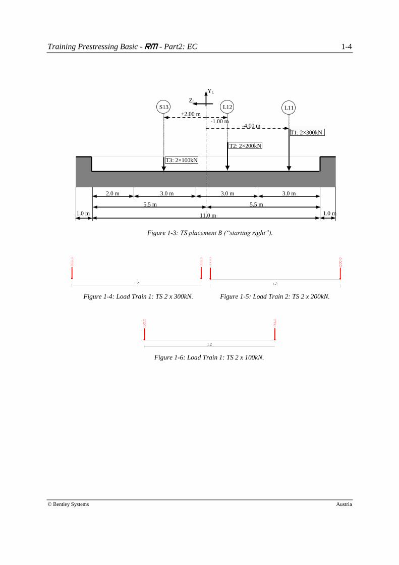
11.0 m 1.0 m 1.0 m
3.0 m
5.5 m 5.5 m
3.0 m
T2: 2×200kN
L11
-1.00 m -4.00 m
+2.00 m
YL
ZL
T1: 2×300kN
3.0 m 2.0 m
T3: 2×100kN
L12 S13
Figure 1-3: TS placement B (“starting right”).
Figure 1-4: Load Train 1: TS 2 x 300kN. Figure 1-5: Load Train 2: TS 2 x 200kN.
Figure 1-6: Load Train 1: TS 2 x 100kN.
Training Prestressing Basic - RM - Part2: EC 1-5
© Bentley Systems Austria
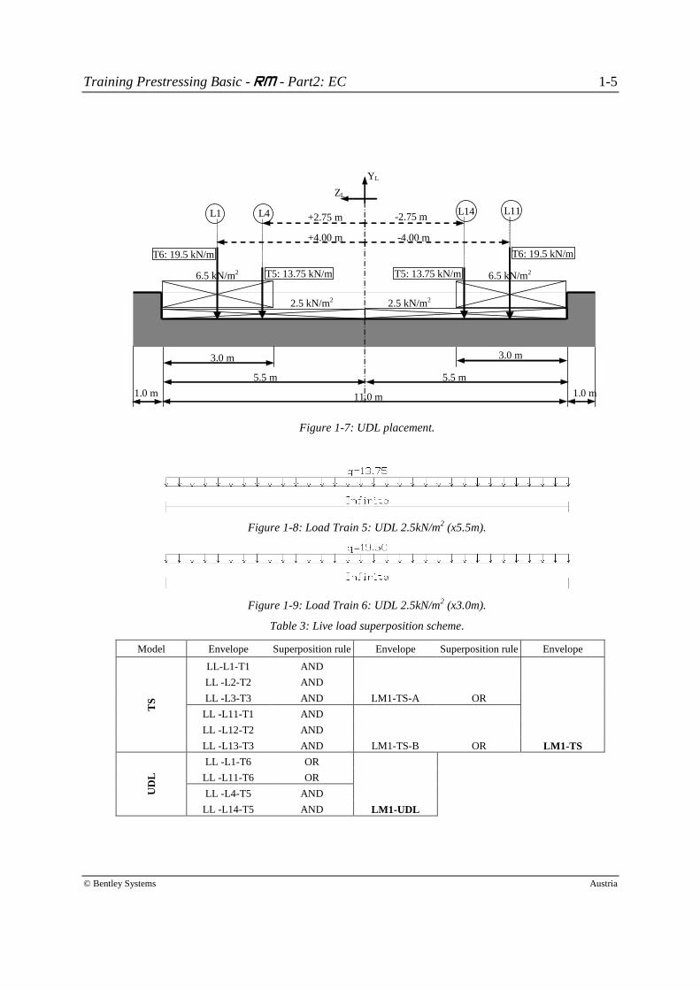
11.0 m 1.0 m 1.0 m
3.0 m
6.5 kN/m2
5.5 m 5.5 m
3.0 m
6.5 kN/m2
2.5 kN/m2 2.5 kN/m2
T5: 13.75 kN/m
L1 L4 L14 L11 +2.75 m
+4.00 m
-2.75 m
-4.00 m
YL
ZL
T6: 19.5 kN/m
T5: 13.75 kN/m
T6: 19.5 kN/m
Figure 1-7: UDL placement.
Figure 1-8: Load Train 5: UDL 2.5kN/m2 (x5.5m).
Figure 1-9: Load Train 6: UDL 2.5kN/m2 (x3.0m).
Table 3: Live load superposition scheme.
Model Envelope Superposition rule Envelope Superposition rule Envelope
TS
LL-L1-T1 AND
LL -L2-T2 AND
LL -L3-T3 AND LM1-TS-A OR
LL -L11-T1 AND
LL -L12-T2 AND
LL -L13-T3 AND LM1-TS-B OR LM1-TS
UD
L
LL -L1-T6 OR
LL -L11-T6 OR
LL -L4-T5 AND
LL -L14-T5 AND LM1-UDL
Training Prestressing Basic - RM - Part2: EC 1-6
© Bentley Systems Austria
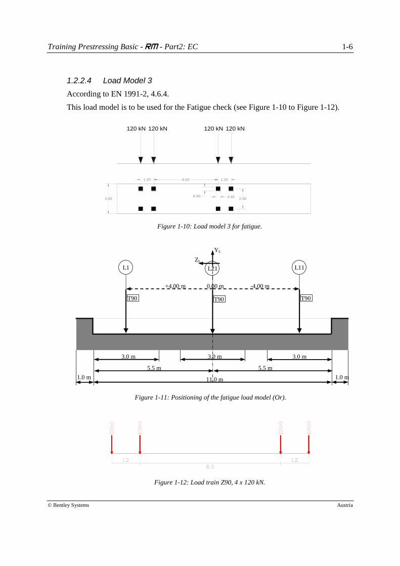
3.00 2.00
1.20 6.00 1.20
120 kN 120 kN 120 kN 120 kN
0.400.40
1.2.2.4 Load Model 3
According to EN 1991-2, 4.6.4.
This load model is to be used for the Fatigue check (see Figure 1-10 to Figure 1-12).
Figure 1-10: Load model 3 for fatigue.
11.0 m 1.0 m 1.0 m
3.0 m
5.5 m 5.5 m
3.0 m
L11
-4.00 m
YL
ZL
T90
L1
T90
+4.00 m
L21
T90
0.00 m
3.0 m
Figure 1-11: Positioning of the fatigue load model (Or).
Figure 1-12: Load train Z90, 4 x 120 kN.
Training Prestressing Basic - RM - Part2: EC 1-7
© Bentley Systems Austria
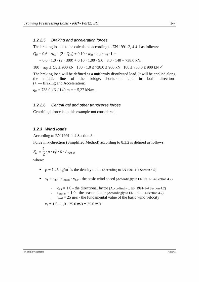
1.2.2.5 Braking and acceleration forces
The braking load is to be calculated according to EN 1991-2, 4.4.1 as follows:
Qlk = 0.6 · Q1 · (2 · Q1k) + 0.10 · q1 · q1k · wl · L =
= 0.6 · 1.0 · (2 · 300) + 0.10 · 1.00 · 9.0 · 3.0 · 140 = 738.0 kN.
180 · Q1 Qlk 900 kN 180 · 1.0 738.0 900 kN 180 738.0 900 kN
The braking load will be defined as a uniformly distributed load. It will be applied along
the middle line of the bridge, horizontal and in both directions
(± → Braking and Acceleration).
qlk = 738.0 kN / 140 m = ± 5,27 kN/m.
1.2.2.6 Centrifugal and other transverse forces
Centrifugal force is in this example not considered.
1.2.3 Wind loads
According to EN 1991-1-4 Section 8.
Force in x-direction (Simplified Method) according to 8.3.2 is defined as follows:
where:
1.25 kg/m3 is the density of air (According to EN 1991-1-4 Section 4.5)
vb = cdir · cseason · vb,0 - the basic wind speed (Accordingly to EN 1991-1-4 Section 4.2)
- cdir = 1.0 - the directional factor (Accordingly to EN 1991-1-4 Section 4.2)
- cseason = 1.0 - the season factor (Accordingly to EN 1991-1-4 Section 4.2)
- vb,0 = 25 m/s - the fundamental value of the basic wind velocity
vb = 1,0 · 1,0 · 25.0 m/s = 25.0 m/s
Training Prestressing Basic - RM - Part2: EC 1-8
© Bentley Systems Austria
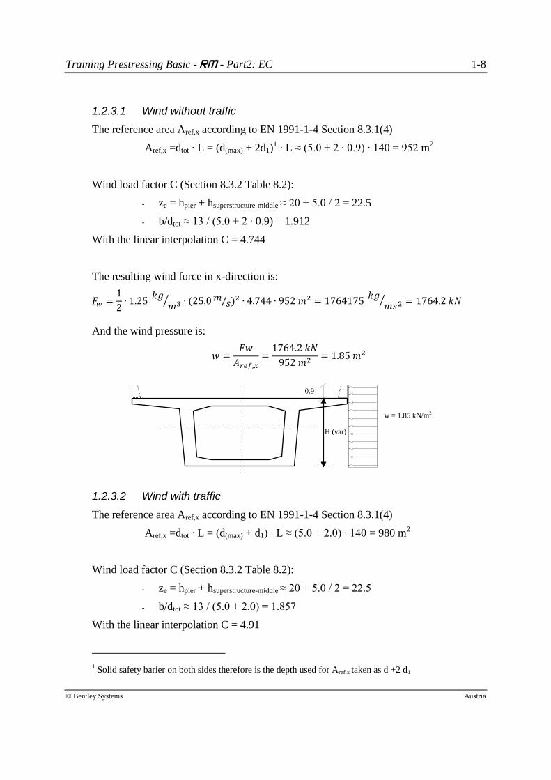
1.2.3.1 Wind without traffic
The reference area Aref,x according to EN 1991-1-4 Section 8.3.1(4)
Aref,x =dtot ∙ L = (d(max) + 2d1)1 ∙ L ≈ (5.0 + 2 ∙ 0.9) ∙ 140 = 952 m
2
Wind load factor C (Section 8.3.2 Table 8.2):
- ze = hpier + hsuperstructure-middle ≈ 20 + 5.0 / 2 = 22.5
- b/dtot ≈ 13 / (5.0 + 2 ∙ 0.9) = 1.912
With the linear interpolation C = 4.744
The resulting wind force in x-direction is:
And the wind pressure is:
1.2.3.2 Wind with traffic
The reference area Aref,x according to EN 1991-1-4 Section 8.3.1(4)
Aref,x =dtot ∙ L = (d(max) + d1) ∙ L ≈ (5.0 + 2.0) ∙ 140 = 980 m2
Wind load factor C (Section 8.3.2 Table 8.2):
- ze = hpier + hsuperstructure-middle ≈ 20 + 5.0 / 2 = 22.5
- b/dtot ≈ 13 / (5.0 + 2.0) = 1.857
With the linear interpolation C = 4.91
1 Solid safety barier on both sides therefore is the depth used for Aref,x taken as d +2 d1
w = 1.85 kN/m2
H (var)
0.9
m
Training Prestressing Basic - RM - Part2: EC 1-9
© Bentley Systems Austria
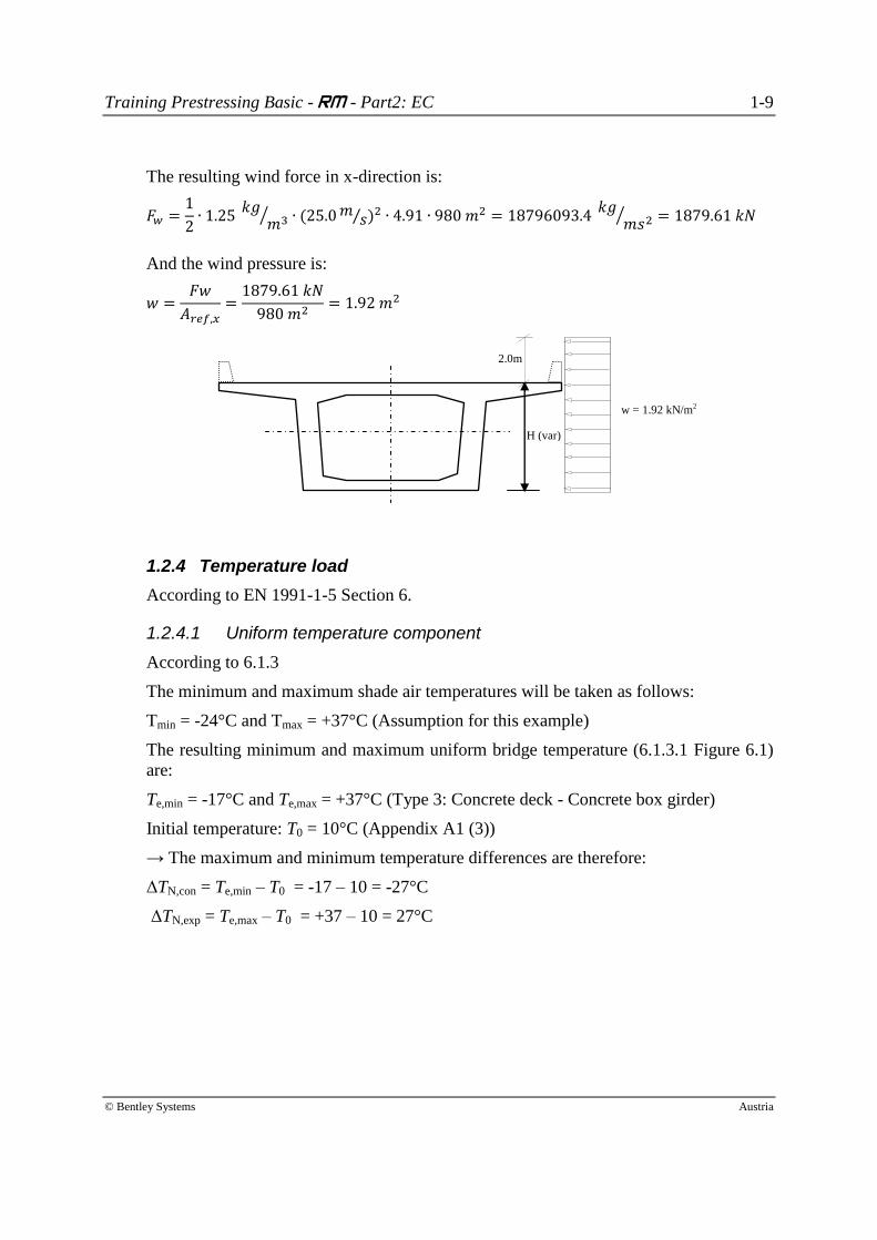
The resulting wind force in x-direction is:
And the wind pressure is:
1.2.4 Temperature load
According to EN 1991-1-5 Section 6.
1.2.4.1 Uniform temperature component
According to 6.1.3
The minimum and maximum shade air temperatures will be taken as follows:
Tmin = -24°C and Tmax = +37°C (Assumption for this example)
The resulting minimum and maximum uniform bridge temperature (6.1.3.1 Figure 6.1)
are:
Te,min = -17°C and Te,max = +37°C (Type 3: Concrete deck - Concrete box girder)
Initial temperature: T0 = 10°C (Appendix A1 (3))
→ The maximum and minimum temperature differences are therefore:
ΔTN,con = Te,min – T0 = -17 – 10 = -27°C
ΔTN,exp = Te,max – T0 = +37 – 10 = 27°C
w = 1.92 kN/m2
H (var)
2.0m
Training Prestressing Basic - RM - Part2: EC 1-10
© Bentley Systems Austria
1.2.4.2 Temperature difference components
According to 6.1.4.1 (Vertical linear component (Approach 1)).
For road bridges of type 3 with a concrete box girder as the superstructure and with a
depth of surfacing of 120 mm the values of linear temperature difference are as follows
(considering the table 6.1 and the corrections factors from table 6.2):
TM,cool = TM,cool,50mm · ksur,120mm = -5 °C · 1.0 = -5 °C
TM,heat = TM,heat,50mm · ksur,120mm = 10 °C · 0.62 = 6.2 °C
1.2.4.3 Combination of uniform temperature component and temperature dif-ference component
The unfavorable component has to be considered:
TM,heat (or TM,cool) + 0.35 · ΔTN,exp (or ΔTN,con)
or
0.75 · TM,heat (or TM,cool) + ΔTN,exp (or ΔTN,con)
This will be taken into account via superposition of each temperature component.
1.2.5 Settlements
For all 4 Axes a pier settlement of 1.0 cm will be assumed.
Training Prestressing Basic - RM - Part2: EC 1-11
© Bentley Systems Austria
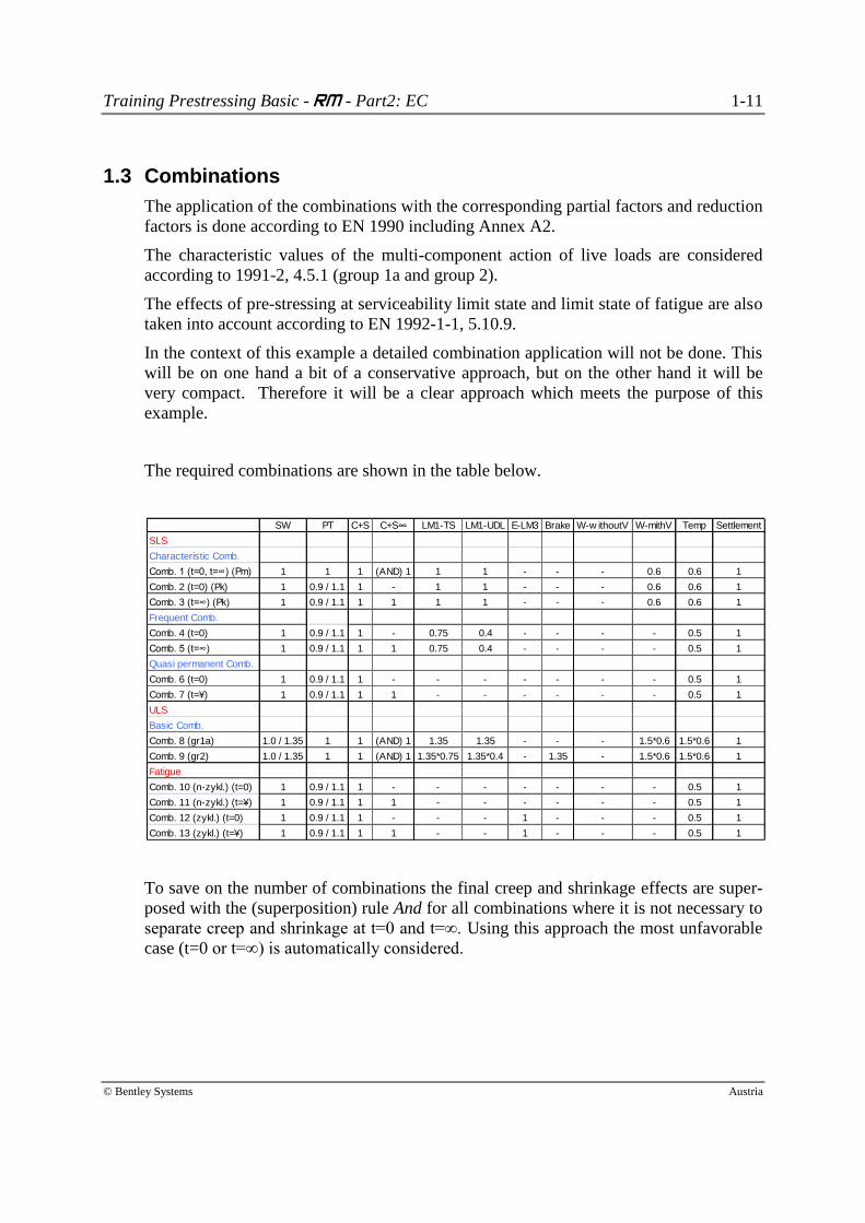
1.3 Combinations
The application of the combinations with the corresponding partial factors and reduction
factors is done according to EN 1990 including Annex A2.
The characteristic values of the multi-component action of live loads are considered
according to 1991-2, 4.5.1 (group 1a and group 2).
The effects of pre-stressing at serviceability limit state and limit state of fatigue are also
taken into account according to EN 1992-1-1, 5.10.9.
In the context of this example a detailed combination application will not be done. This
will be on one hand a bit of a conservative approach, but on the other hand it will be
very compact. Therefore it will be a clear approach which meets the purpose of this
example.
The required combinations are shown in the table below.
To save on the number of combinations the final creep and shrinkage effects are super-
posed with the (superposition) rule And for all combinations where it is not necessary to
separate creep and shrinkage at t=0 and t=∞. Using this approach the most unfavorable
case (t=0 or t=∞) is automatically considered.
SW PT C+S C+S∞ LM1-TS LM1-UDL E-LM3 Brake W-w ithoutV W-mithV Temp Settlement
SLS
Characteristic Comb.
Comb. 1 (t=0, t=∞) (Pm) 1 1 1 (AND) 1 1 1 - - - 0.6 0.6 1
Comb. 2 (t=0) (Pk) 1 0.9 / 1.1 1 - 1 1 - - - 0.6 0.6 1
Comb. 3 (t=∞) (Pk) 1 0.9 / 1.1 1 1 1 1 - - - 0.6 0.6 1
Frequent Comb.
Comb. 4 (t=0) 1 0.9 / 1.1 1 - 0.75 0.4 - - - - 0.5 1
Comb. 5 (t=∞) 1 0.9 / 1.1 1 1 0.75 0.4 - - - - 0.5 1
Quasi permanent Comb.
Comb. 6 (t=0) 1 0.9 / 1.1 1 - - - - - - - 0.5 1
Comb. 7 (t=¥) 1 0.9 / 1.1 1 1 - - - - - - 0.5 1
ULS
Basic Comb.
Comb. 8 (gr1a) 1.0 / 1.35 1 1 (AND) 1 1.35 1.35 - - - 1.5*0.6 1.5*0.6 1
Comb. 9 (gr2) 1.0 / 1.35 1 1 (AND) 1 1.35*0.75 1.35*0.4 - 1.35 - 1.5*0.6 1.5*0.6 1
Fatigue
Comb. 10 (n-zykl.) (t=0) 1 0.9 / 1.1 1 - - - - - - - 0.5 1
Comb. 11 (n-zykl.) (t=¥) 1 0.9 / 1.1 1 1 - - - - - - 0.5 1
Comb. 12 (zykl.) (t=0) 1 0.9 / 1.1 1 - - - 1 - - - 0.5 1
Comb. 13 (zykl.) (t=¥) 1 0.9 / 1.1 1 1 - - 1 - - - 0.5 1
Training Prestressing Basic - RM - Part2: EC 1-12
© Bentley Systems Austria
1.4 Design checks
According to EN 1992-1-1 Section 6 and 7 and EN 1992-2 Section 6 and 7.
1.4.1 Servicebility limit state
Accordingly to EN 1992-1-1, 7.1(2) the cross-sections should be assumed to be
un-cracked if the flexural tensile stress does not exceed fctm.
1.4.1.1 Stresses
Accordingly to EN 1992-1-1, 7.2 and 1992-2 7.2.
Concrete compressive stresses
For prevention of longitudinal cracking, which can lead to reduction of durability, the
compressive stresses are limited to
|σc| 0.6 · |fck| under the characteristic combination for the exposure classes
XD, XF and XS.
Linear creep may be assumed for
|σc| 0.45 · |fck| under the characteristic combination.
Non-linear creep should be considered for
|σc| > 0.45 · |fck| under the quasi permanent combination.
Reinforcement tensile stresses
σs 0.80 · fyk for the characteristic combination.
Stress in pre-stressing tendons
σp 0.75 · fpk for the characteristic combination.
Training Prestressing Basic - RM - Part2: EC 1-13
© Bentley Systems Austria
1.4.1.2 Crack control
According to EN1992-1-1, 7.3 and 1992-2, 7.3.
Limiting calculated crack
wact wmax wmax = 0.20 mm for frequent load combination
Decompression
σc 0 for the quasi-permanent load combination
The decompression limit requires that all parts of the tendons
or duct lie at least 25 mm within concrete in compression.
Minimum reinforcement area
σc ≥ fctm for the frequent load combination
1.4.2 Ultimate limit state
Accordingly to EN 1992-1-1 and 1992-2 section 6.
Design checks to be made:
Bending and axial force
Shear
Torsion
Fatigue
Training Prestressing Basic - RM - Part2: EC 2-14
© Bentley Systems Austria
2 Lesson 13: Definition of Additional Loads
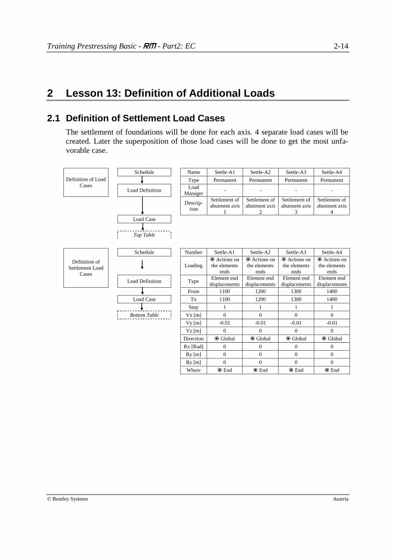
2.1 Definition of Settlement Load Cases
The settlement of foundations will be done for each axis. 4 separate load cases will be
created. Later the superposition of those load cases will be done to get the most unfa-
vorable case.
Definition of Load
Cases
Schedule Name Settle-A1 Settle-A2 Settle-A3 Settle-A4
Type Permanent Permanent Permanent Permanent
Load Definition Load
Manager - - - -
Descrip-
tion
Settlement of
abutment axis
1
Settlement of
abutment axis
2
Settlement of
abutment axis
3
Settlement of
abutment axis
4
Load Case
Top Table
Definition of
Settlement Load Cases
Schedule Number Settle-A1 Settle-A2 Settle-A3 Settle-A4
Loading Actions on the elements
ends
Actions on the elements
ends
Actions on the elements
ends
Actions on the elements
ends
Load Definition Type Element end
displacements
Element end
displacements
Element end
displacements
Element end
displacements
From 1100 1200 1300 1400
Load Case To 1100 1200 1300 1400
Step 1 1 1 1
Bottom Table Vx [m] 0 0 0 0
Vy [m] -0.01 -0.01 -0.01 -0.01
Vz [m] 0 0 0 0
Direction Global Global Global Global
Rx [Rad] 0 0 0 0
Ry [m] 0 0 0 0
Rz [m] 0 0 0 0
Where End End End End
Training Prestressing Basic - RM - Part2: EC 2-15
© Bentley Systems Austria
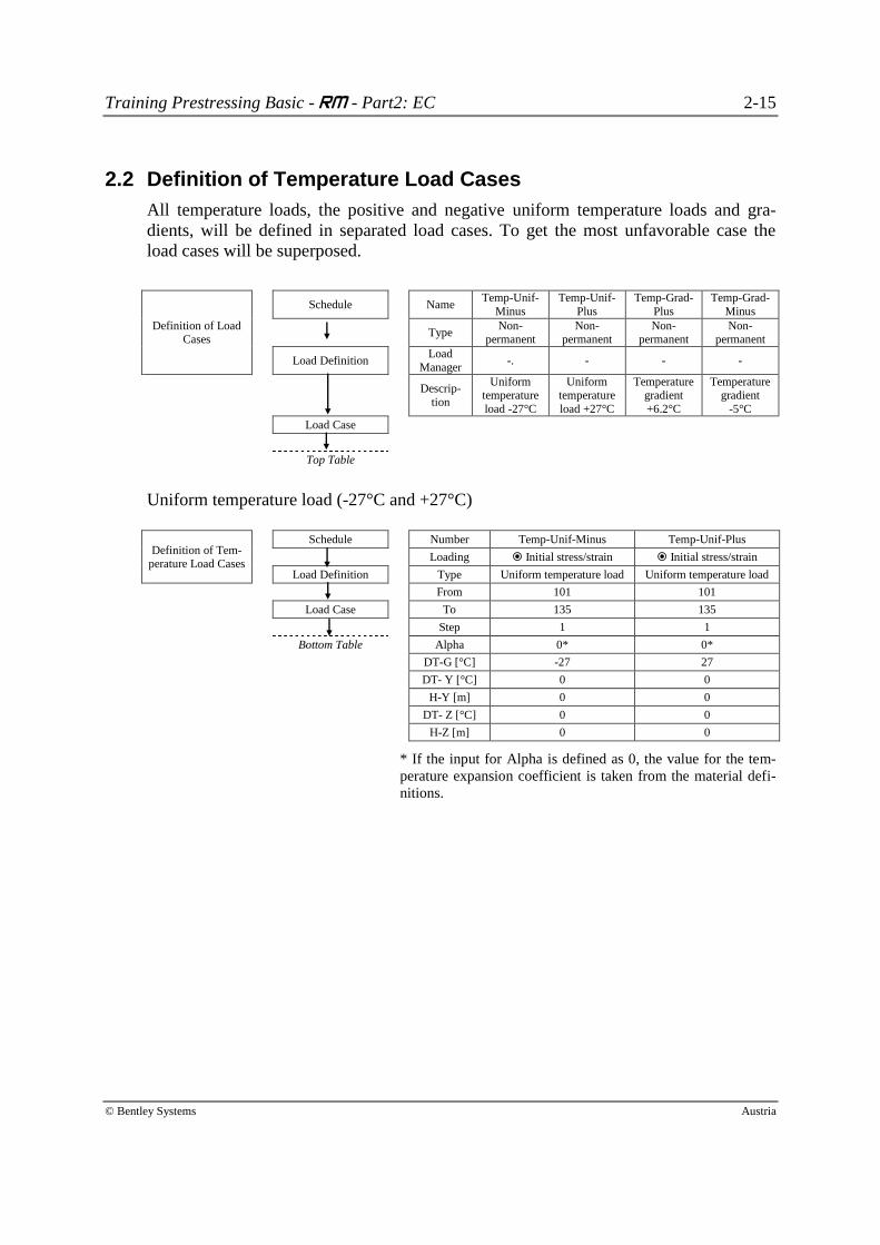
2.2 Definition of Temperature Load Cases
All temperature loads, the positive and negative uniform temperature loads and gra-
dients, will be defined in separated load cases. To get the most unfavorable case the
load cases will be superposed.
Definition of Load
Cases
Schedule Name Temp-Unif-
Minus
Temp-Unif-
Plus
Temp-Grad-
Plus
Temp-Grad-
Minus
Type Non-
permanent
Non-
permanent
Non-
permanent
Non-
permanent
Load Definition Load
Manager -. - - -
Descrip-
tion
Uniform temperature
load -27°C
Uniform temperature
load +27°C
Temperature gradient
+6.2°C
Temperature gradient
-5°C
Load Case
Top Table
Uniform temperature load (-27°C and +27°C)
Definition of Tem-perature Load Cases
Schedule Number Temp-Unif-Minus Temp-Unif-Plus
Loading Initial stress/strain Initial stress/strain
Load Definition Type Uniform temperature load Uniform temperature load
From 101 101
Load Case To 135 135
Step 1 1
Bottom Table Alpha 0* 0*
DT-G [°C] -27 27
DT- Y [°C] 0 0
H-Y [m] 0 0
DT- Z [°C] 0 0
H-Z [m] 0 0
* If the input for Alpha is defined as 0, the value for the tem-
perature expansion coefficient is taken from the material defi-
nitions.
Training Prestressing Basic - RM - Part2: EC 2-16
© Bentley Systems Austria
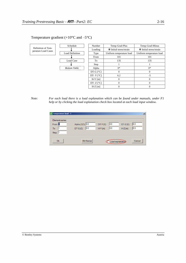
Temperature gradient (+10°C and –5°C)
Definition of Tem-perature Load Cases
Schedule Number Temp-Grad-Plus Temp-Grad-Minus
Loading Initial stress/strain Initial stress/strain
Load Definition Type Uniform temperature load Uniform temperature load
From 101 101
Load Case To 135 135
Step 1 1
Bottom Table Alpha 0* 0*
DT-G [°C] 0 0
DT- Y [°C] 6.2 -5
H-Y [m] 0 0
DT- Z [°C] 0 0
H-Z [m] 0 0
Note: For each load there is a load explanation which can be found under manuals, under F1
help or by clicking the load explanation check box located at each load input window.
Training Prestressing Basic - RM - Part2: EC 2-17
© Bentley Systems Austria
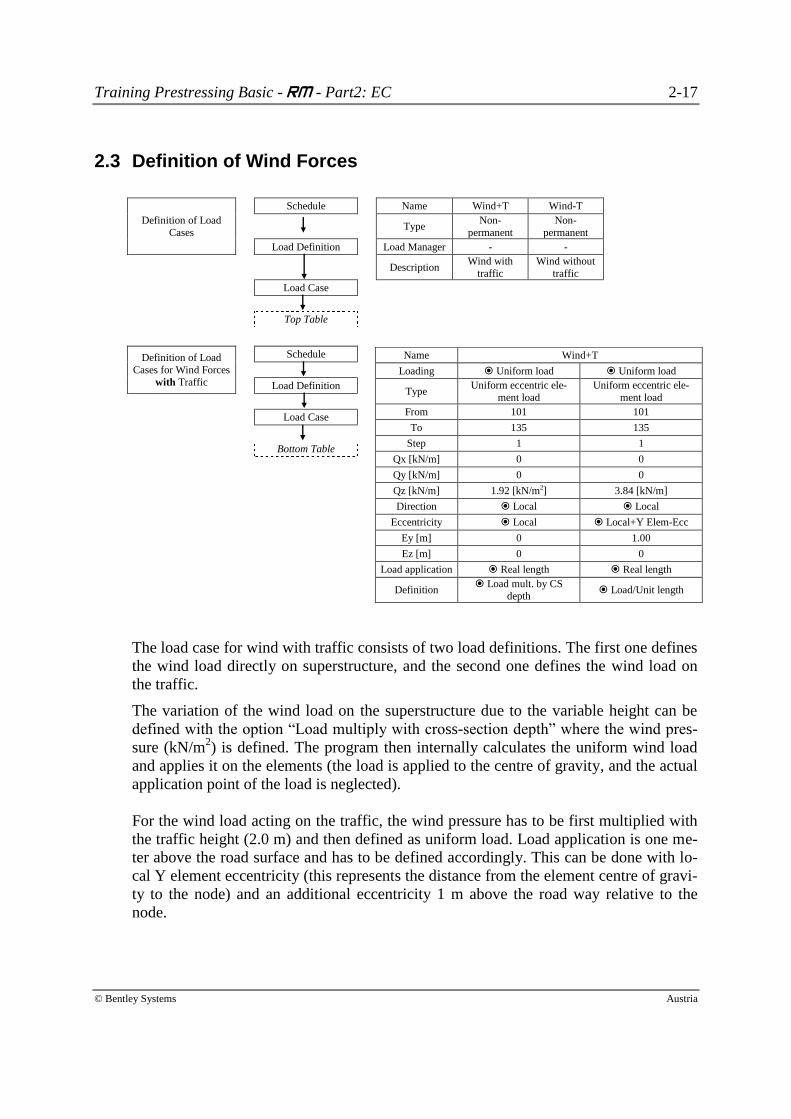
2.3 Definition of Wind Forces
Definition of Load
Cases
Schedule Name Wind+T Wind-T
Type Non-
permanent
Non-
permanent
Load Definition Load Manager - -
Description Wind with
traffic
Wind without
traffic
Load Case
Top Table
Definition of Load
Cases for Wind Forces
with Traffic
Schedule
Load Definition
Load Case
Bottom Table
The load case for wind with traffic consists of two load definitions. The first one defines
the wind load directly on superstructure, and the second one defines the wind load on
the traffic.
The variation of the wind load on the superstructure due to the variable height can be
defined with the option “Load multiply with cross-section depth” where the wind pres-
sure (kN/m2) is defined. The program then internally calculates the uniform wind load
and applies it on the elements (the load is applied to the centre of gravity, and the actual
application point of the load is neglected).
For the wind load acting on the traffic, the wind pressure has to be first multiplied with
the traffic height (2.0 m) and then defined as uniform load. Load application is one me-
ter above the road surface and has to be defined accordingly. This can be done with lo-
cal Y element eccentricity (this represents the distance from the element centre of gravi-
ty to the node) and an additional eccentricity 1 m above the road way relative to the
node.
Name Wind+T
Loading Uniform load Uniform load
Type Uniform eccentric ele-
ment load
Uniform eccentric ele-
ment load
From 101 101
To 135 135
Step 1 1
Qx [kN/m] 0 0
Qy [kN/m] 0 0
Qz [kN/m] 1.92 [kN/m2] 3.84 [kN/m]
Direction Local Local
Eccentricity Local Local+Y Elem-Ecc
Ey [m] 0 1.00
Ez [m] 0 0
Load application Real length Real length
Definition Load mult. by CS
depth Load/Unit length
Training Prestressing Basic - RM - Part2: EC 2-18
© Bentley Systems Austria
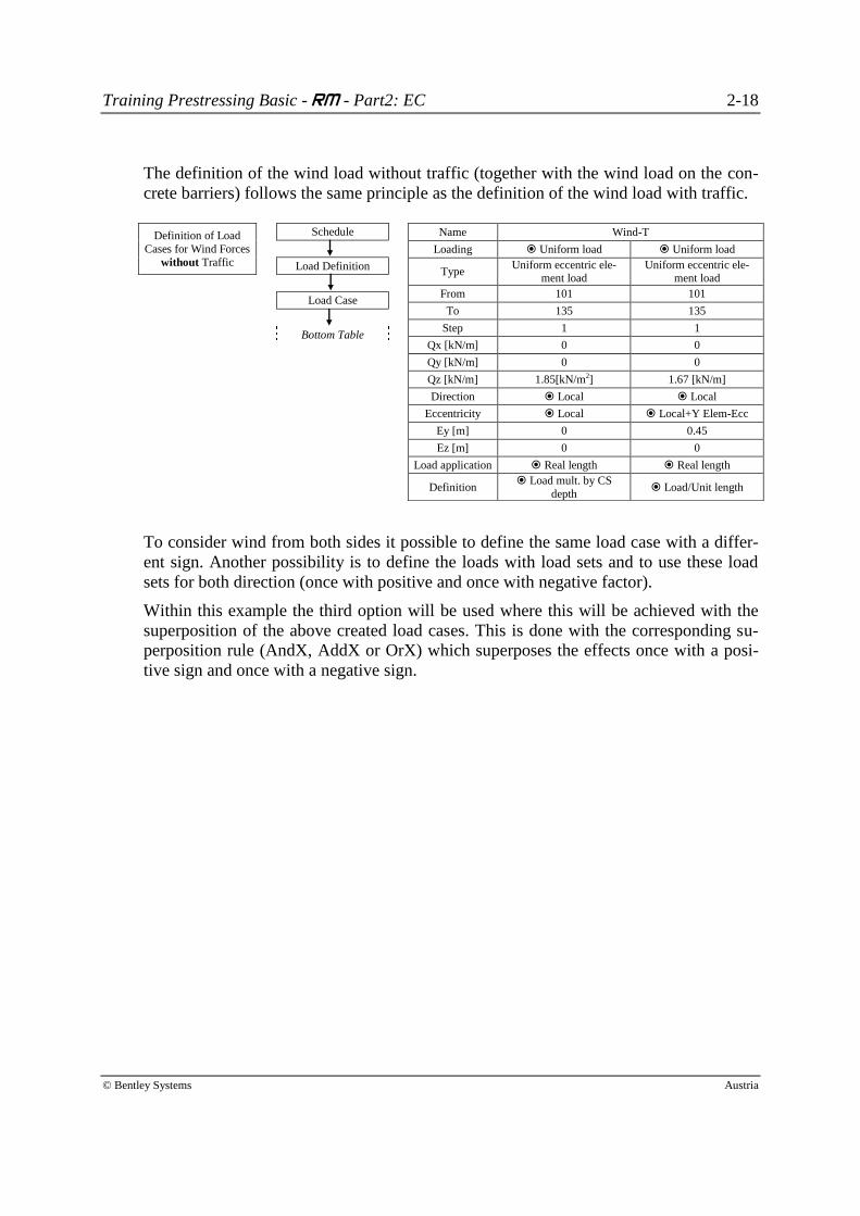
The definition of the wind load without traffic (together with the wind load on the con-
crete barriers) follows the same principle as the definition of the wind load with traffic.
Definition of Load
Cases for Wind Forces
without Traffic
Schedule
Load Definition
Load Case
Bottom Table
To consider wind from both sides it possible to define the same load case with a differ-
ent sign. Another possibility is to define the loads with load sets and to use these load
sets for both direction (once with positive and once with negative factor).
Within this example the third option will be used where this will be achieved with the
superposition of the above created load cases. This is done with the corresponding su-
perposition rule (AndX, AddX or OrX) which superposes the effects once with a posi-
tive sign and once with a negative sign.
Name Wind-T
Loading Uniform load Uniform load
Type Uniform eccentric ele-
ment load Uniform eccentric ele-
ment load
From 101 101
To 135 135
Step 1 1
Qx [kN/m] 0 0
Qy [kN/m] 0 0
Qz [kN/m] 1.85[kN/m2] 1.67 [kN/m]
Direction Local Local
Eccentricity Local Local+Y Elem-Ecc
Ey [m] 0 0.45
Ez [m] 0 0
Load application Real length Real length
Definition Load mult. by CS
depth Load/Unit length
Training Prestressing Basic - RM - Part2: EC 2-19
© Bentley Systems Austria
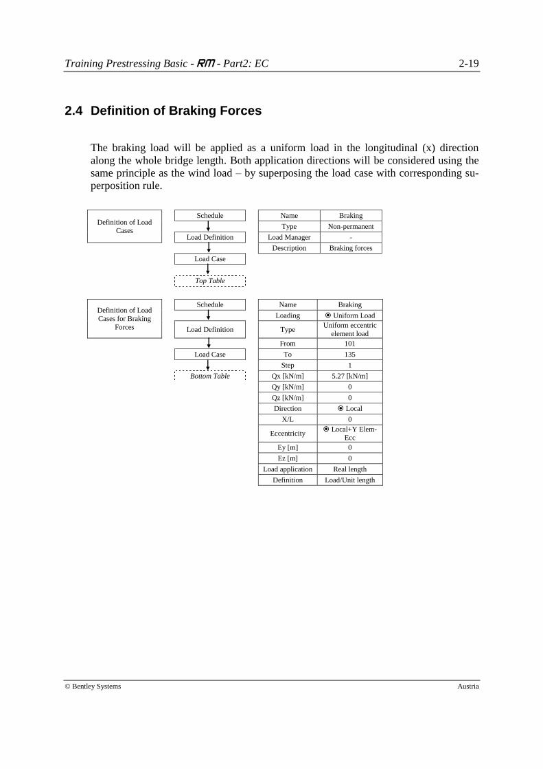
2.4 Definition of Braking Forces
The braking load will be applied as a uniform load in the longitudinal (x) direction
along the whole bridge length. Both application directions will be considered using the
same principle as the wind load – by superposing the load case with corresponding su-
perposition rule.
Definition of Load Cases
Schedule Name Braking
Type Non-permanent
Load Definition Load Manager -
Description Braking forces
Load Case
Top Table
Definition of Load
Cases for Braking
Forces
Schedule Name Braking
Loading Uniform Load
Load Definition Type Uniform eccentric
element load
From 101
Load Case To 135
Step 1
Bottom Table Qx [kN/m] 5.27 [kN/m]
Qy [kN/m] 0
Qz [kN/m] 0
Direction Local
X/L 0
Eccentricity Local+Y Elem-
Ecc
Ey [m] 0
Ez [m] 0
Load application Real length
Definition Load/Unit length
Training Prestressing Basic - RM - Part2: EC 3-20
© Bentley Systems Austria
3 Lesson 14: Calculation and Superposition of additional loads
The arrangement of the subsequent “Construction stages” can be made freely. They are
actually not real construction stages because there will be no elements activated or time
depended calculations made. They will be only recalculation stages. However, it is
recommended to group them with some logical principle.
Each type of additional load will be grouped together – this means that for each a calcu-
lation stage will be generated where the loads will be calculated and superposed into
one envelope. In this envelope the minimum and maximum results will be saved. The
same envelope will be used for the load combinations.
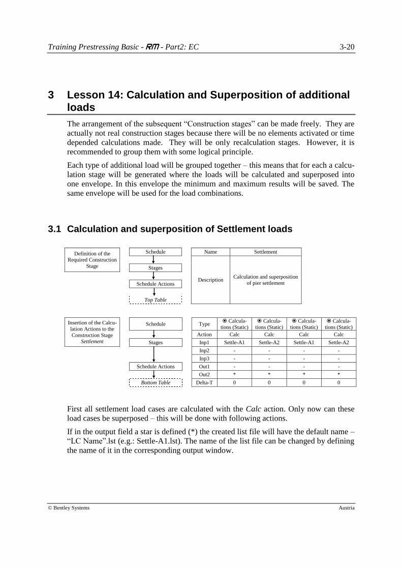
3.1 Calculation and superposition of Settlement loads
Definition of the
Required Construction
Stage
Schedule Name Settlement
Description Calculation and superposition
of pier settlement
Stages
Schedule Actions
Top Table
Insertion of the Calcu-
lation Actions to the
Construction Stage Settlement
Schedule Type Calcula-
tions (Static)
Calcula-
tions (Static)
Calcula-
tions (Static)
Calcula-
tions (Static)
Action Calc Calc Calc Calc
Stages Inp1 Settle-A1 Settle-A2 Settle-A1 Settle-A2
Inp2 - - - -
Inp3 - - - -
Schedule Actions Out1 - - - -
Out2 * * * *
Bottom Table Delta-T 0 0 0 0
First all settlement load cases are calculated with the Calc action. Only now can these
load cases be superposed – this will be done with following actions.
If in the output field a star is defined (*) the created list file will have the default name –
“LC Name”.lst (e.g.: Settle-A1.lst). The name of the list file can be changed by defining
the name of it in the corresponding output window.
Training Prestressing Basic - RM - Part2: EC 3-21
© Bentley Systems Austria
Type LC/Envelop
e action
LC/Envelop
e action
LC/Envelop
e action
LC/Envelop
e action
LC/Envelop
e action
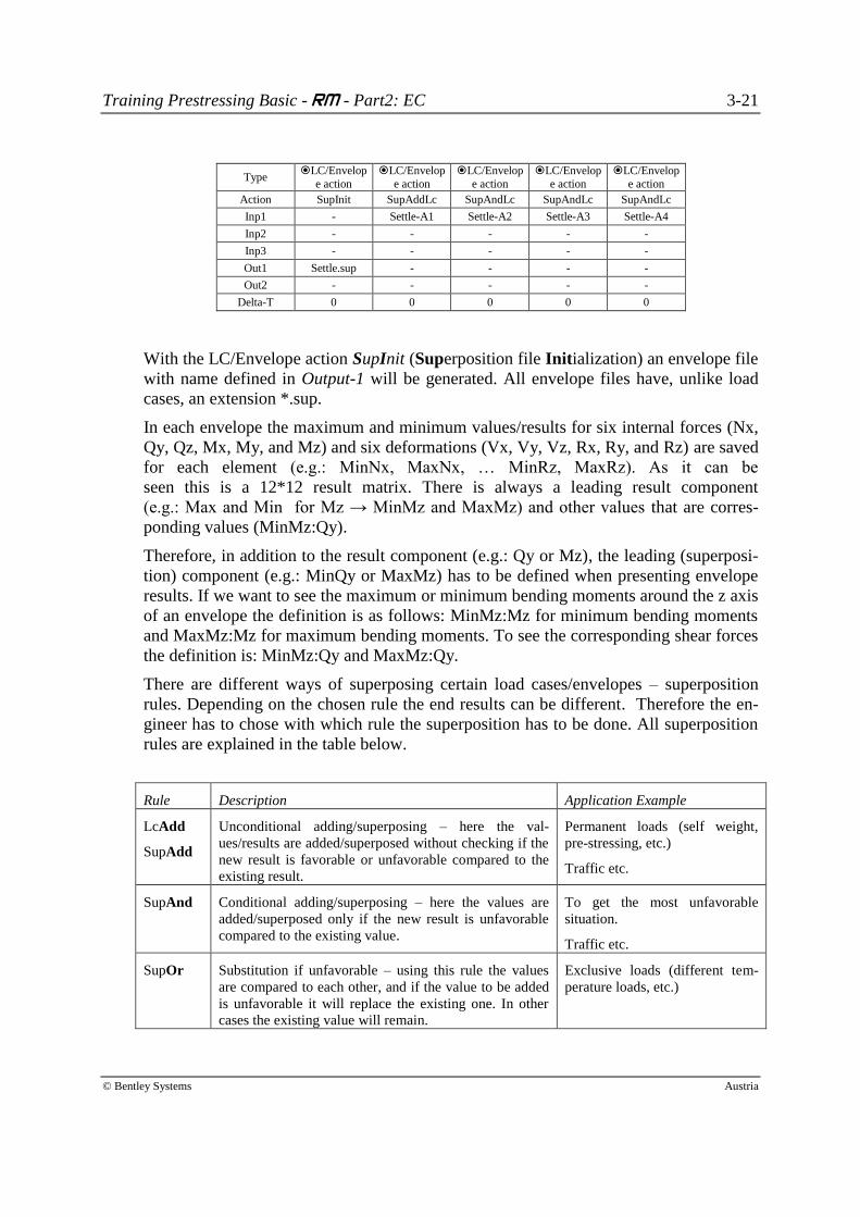
Action SupInit SupAddLc SupAndLc SupAndLc SupAndLc
Inp1 - Settle-A1 Settle-A2 Settle-A3 Settle-A4
Inp2 - - - - -
Inp3 - - - - -
Out1 Settle.sup - - - -
Out2 - - - - -
Delta-T 0 0 0 0 0
With the LC/Envelope action SupInit (Superposition file Initialization) an envelope file
with name defined in Output-1 will be generated. All envelope files have, unlike load
cases, an extension *.sup.
In each envelope the maximum and minimum values/results for six internal forces (Nx,
Qy, Qz, Mx, My, and Mz) and six deformations (Vx, Vy, Vz, Rx, Ry, and Rz) are saved
for each element (e.g.: MinNx, MaxNx, … MinRz, MaxRz). As it can be
seen this is a 12*12 result matrix. There is always a leading result component
(e.g.: Max and Min for Mz → MinMz and MaxMz) and other values that are corres-
ponding values (MinMz:Qy).
Therefore, in addition to the result component (e.g.: Qy or Mz), the leading (superposi-
tion) component (e.g.: MinQy or MaxMz) has to be defined when presenting envelope
results. If we want to see the maximum or minimum bending moments around the z axis
of an envelope the definition is as follows: MinMz:Mz for minimum bending moments
and MaxMz:Mz for maximum bending moments. To see the corresponding shear forces
the definition is: MinMz:Qy and MaxMz:Qy.
There are different ways of superposing certain load cases/envelopes – superposition
rules. Depending on the chosen rule the end results can be different. Therefore the en-
gineer has to chose with which rule the superposition has to be done. All superposition
rules are explained in the table below.
Rule Description Application Example
LcAdd
SupAdd
Unconditional adding/superposing – here the val-
ues/results are added/superposed without checking if the
new result is favorable or unfavorable compared to the
existing result.
Permanent loads (self weight,
pre-stressing, etc.)
Traffic etc.
SupAnd Conditional adding/superposing – here the values are
added/superposed only if the new result is unfavorable
compared to the existing value.
To get the most unfavorable
situation.
Traffic etc.
SupOr Substitution if unfavorable – using this rule the values
are compared to each other, and if the value to be added
is unfavorable it will replace the existing one. In other
cases the existing value will remain.
Exclusive loads (different tem-
perature loads, etc.)
Training Prestressing Basic - RM - Part2: EC 3-22
© Bentley Systems Austria
SupAndX Both have the same functionality as their basic rules
(SupAnd and SurOr). The difference is that the values to
be added are superposed once with positive factor (+1)
and once time with negative factor (-1).
Wind loads and Braking loads
which are defined only from one
side. SupOrX
Depending on the file to be added, load case or envelope, there are different actions –
SupAndLc or SupAndSup.
For further and more detailed information about the superposition rules see the RM
Bridge Analysis User Guide, Section 7.2.5.
In this particular example (Settlement of each axis) the values are conditionally super-
posed with the actions SupAndLc (to the Settle envelope a load case will be added with
the rule And – conditional adding). This means that individual result components (Nx,
Qy, … Mz) are added only if the respective maximum or minimum result value be-
comes unfavorable.
Note: By the definition of the envelope file (Output 1) using the SupInit action the extension
doesn’t have to be defined because it will be automatically added. This doesn’t apply for all
other superposition actions – it is necessary to write the extension (or selection from the
drop down menu).
Selecting the envelope from the drop down menu is possible only if the envelope already
exists (that it was created/initialized). To avoid a complete recalculation, the action for
creating the envelope can be started separately by clicking the Run Action button on the
right side between the top and bottom table. By clicking on it a new window opens where
the Run Action button has to be clicked and the currently selected action will be performed.
Using this principle the created envelope can be selected from the drop down menu.
For easier and faster definition the action can be copied and modified. The input can also
be defined by the copy-paste function.
Training Prestressing Basic - RM - Part2: EC 3-23
© Bentley Systems Austria
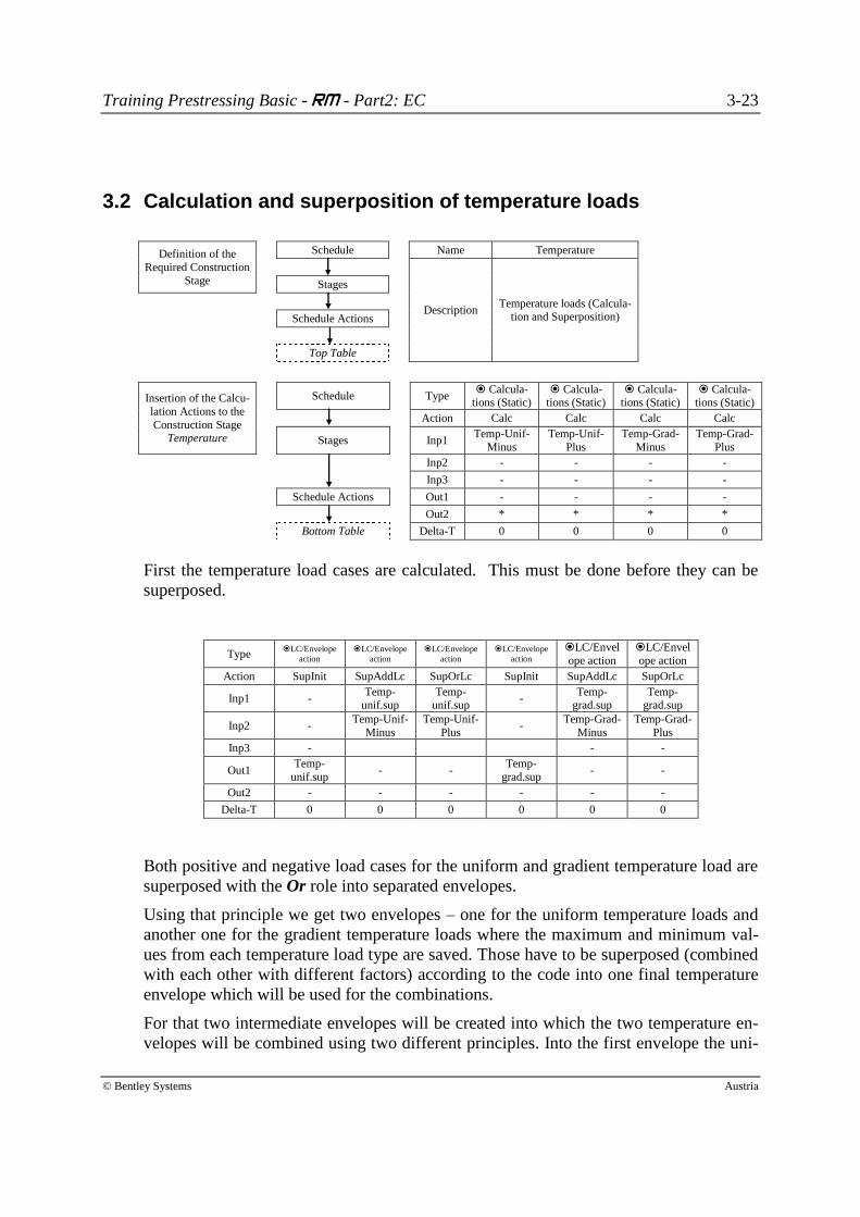
3.2 Calculation and superposition of temperature loads
Definition of the
Required Construction
Stage
Schedule Name Temperature
Description Temperature loads (Calcula-
tion and Superposition)
Stages
Schedule Actions
Top Table
Insertion of the Calcu-
lation Actions to the
Construction Stage Temperature
Schedule Type Calcula-
tions (Static) Calcula-
tions (Static) Calcula-
tions (Static) Calcula-
tions (Static)
Action Calc Calc Calc Calc
Stages Inp1 Temp-Unif-
Minus
Temp-Unif-
Plus
Temp-Grad-
Minus
Temp-Grad-
Plus
Inp2 - - - -
Inp3 - - - -
Schedule Actions Out1 - - - -
Out2 * * * *
Bottom Table Delta-T 0 0 0 0
First the temperature load cases are calculated. This must be done before they can be
superposed.
Type LC/Envelope
action
LC/Envelope
action
LC/Envelope
action
LC/Envelope
action
LC/Envel
ope action
LC/Envel
ope action
Action SupInit SupAddLc SupOrLc SupInit SupAddLc SupOrLc
Inp1 - Temp-
unif.sup Temp-
unif.sup -
Temp-grad.sup
Temp-grad.sup
Inp2 - Temp-Unif-
Minus
Temp-Unif-
Plus -
Temp-Grad-
Minus
Temp-Grad-
Plus
Inp3 - - -
Out1 Temp-
unif.sup - -
Temp-
grad.sup - -
Out2 - - - - - -
Delta-T 0 0 0 0 0 0
Both positive and negative load cases for the uniform and gradient temperature load are
superposed with the Or role into separated envelopes.
Using that principle we get two envelopes – one for the uniform temperature loads and
another one for the gradient temperature loads where the maximum and minimum val-
ues from each temperature load type are saved. Those have to be superposed (combined
with each other with different factors) according to the code into one final temperature
envelope which will be used for the combinations.
For that two intermediate envelopes will be created into which the two temperature en-
velopes will be combined using two different principles. Into the first envelope the uni-
Training Prestressing Basic - RM - Part2: EC 3-24
© Bentley Systems Austria
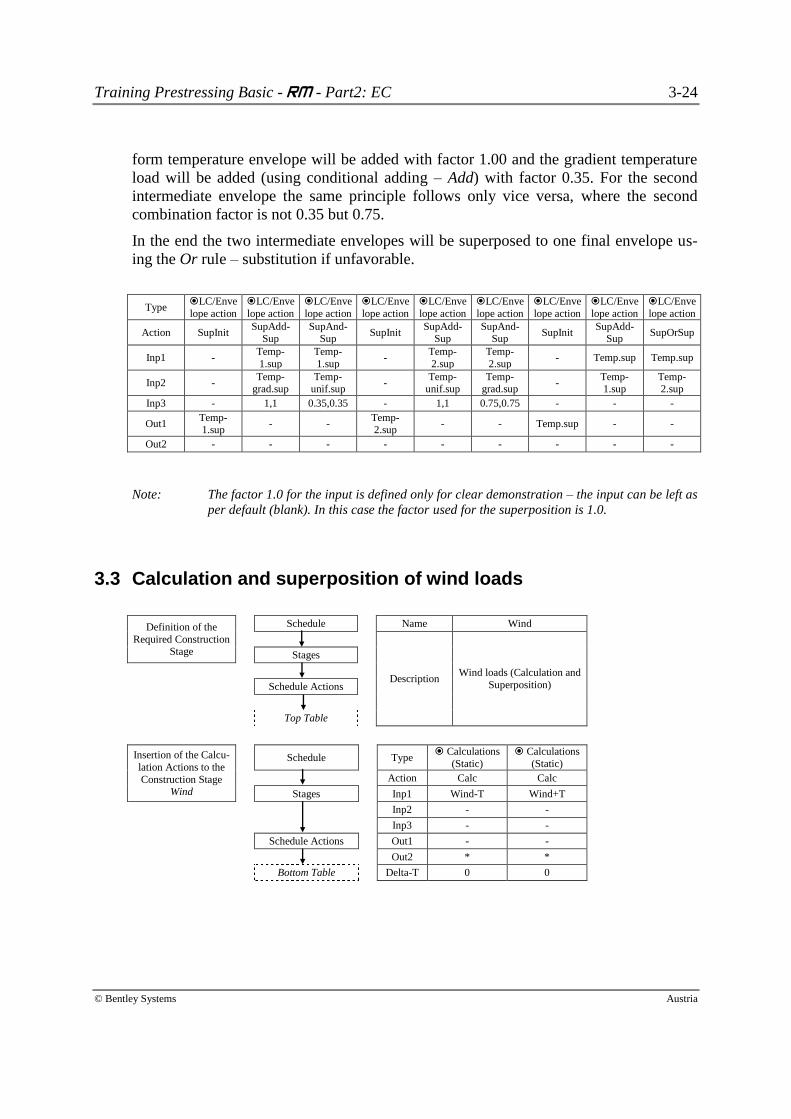
form temperature envelope will be added with factor 1.00 and the gradient temperature
load will be added (using conditional adding – Add) with factor 0.35. For the second
intermediate envelope the same principle follows only vice versa, where the second
combination factor is not 0.35 but 0.75.
In the end the two intermediate envelopes will be superposed to one final envelope us-
ing the Or rule – substitution if unfavorable.
Type LC/Enve
lope action
LC/Enve
lope action
LC/Enve
lope action
LC/Enve
lope action
LC/Enve
lope action
LC/Enve
lope action
LC/Enve
lope action
LC/Enve
lope action
LC/Enve
lope action
Action SupInit SupAdd-
Sup SupAnd-
Sup SupInit
SupAdd-Sup
SupAnd-Sup
SupInit SupAdd-
Sup SupOrSup
Inp1 - Temp-
1.sup
Temp-
1.sup -
Temp-
2.sup
Temp-
2.sup - Temp.sup Temp.sup
Inp2 - Temp-
grad.sup Temp-
unif.sup -
Temp-unif.sup
Temp-grad.sup
- Temp-1.sup
Temp-2.sup
Inp3 - 1,1 0.35,0.35 - 1,1 0.75,0.75 - - -
Out1 Temp-1.sup
- - Temp-2.sup
- - Temp.sup - -
Out2 - - - - - - - - -
Note: The factor 1.0 for the input is defined only for clear demonstration – the input can be left as
per default (blank). In this case the factor used for the superposition is 1.0.
3.3 Calculation and superposition of wind loads
Definition of the
Required Construction Stage
Schedule Name Wind
Description Wind loads (Calculation and
Superposition)
Stages
Schedule Actions
Top Table
Insertion of the Calcu-
lation Actions to the
Construction Stage Wind
Schedule Type Calculations
(Static)
Calculations
(Static)
Action Calc Calc
Stages Inp1 Wind-T Wind+T
Inp2 - -
Inp3 - -
Schedule Actions Out1 - -
Out2 * *
Bottom Table Delta-T 0 0
Training Prestressing Basic - RM - Part2: EC 3-25
© Bentley Systems Austria
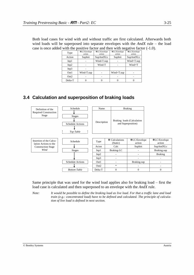
Both load cases for wind with and without traffic are first calculated. Afterwards both
wind loads will be superposed into separate envelopes with the AndX rule – the load
case is once added with the positive factor and then with negative factor (-1.0). Type
LC/Envelope
action
LC/Envelope
action
LC/Envelope
action
LC/Envelope
action
Action SupInit SupAndXLc SupInit SupAndXLc
Inp1 - Wind-T.sup - Wind+T.sup
Inp2 - Wind-T - Wind+T
Inp3 -
Out1 Wind-T.sup - Wind+T.sup -
Out2 - - - -
Delta-T 0 0 0 0
3.4 Calculation and superposition of braking loads
Definition of the
Required Construction Stage
Schedule Name Braking
Description Braking loads (Calculation
and Superposition)
Stages
Schedule Actions
Top Table
Insertion of the Calcu-
lation Actions to the
Construction Stage Wind
Schedule Type Calculations
(Static)
LC/Envelope
action
LC/Envelope
action
Acion Calc SupInit SupAndXLc
Stages Inp1 Braking-LC - Braking.sup
Inp2 - - Braking
Inp3 - - -
Schedule Actions Out1 - Braking.sup -
Out2 * - -
Bottom Table Delta-T 0 0 0
Same principle that was used for the wind load applies also for braking load – first the
load case is calculated and then superposed to an envelope with the AndX rule.
Note: It would be possible to define the braking load as live load. For that a traffic lane and load
train (e.g.: concentrated load) have to be defined and calculated. The principle of calcula-
tion of live load is defined in next section.
Training Prestressing Basic - RM - Part2: EC 4-26
© Bentley Systems Austria
4 Lesson 15: Traffic Loads
The definition and calculation of live loads is done differently than other loads. Instead
of load cases Traffic lanes and Load trains have to be defined. First the traffic lines are
evaluated in schedule actions – influence lines are calculated. Then the load trains are
combined with traffic lanes, and the results are saved into envelopes which are super-
posed into the final envelope(s).
The procedure is outlined below:
Load definition
1) Definition of traffic lanes (Schedule Load definition Traffic Lanes) via
different macros.
2) Definition of load trains (Schedule Load definition Load Trains) using
concentrated loads and uniform loads with fixed and unfixed length.
Schedule actions
3) Evaluation of Traffic Lanes – calculation of influence lines (Action Infl).
4) Initialization of envelopes used for evaluating load trains on influence lines (Ac-
tion SupInit).
5) Evaluation of load trains and influence lines (Action LiveL). The results are
saved into the previously created envelopes.
6) Superposition of envelopes where individual results of the evaluation are stored
to get the combination of (different) load trains in different positions. The final
result of the superposition is/are envelope(s) which is/are used later during the
calculation of combinations.
Training Prestressing Basic - RM - Part2: EC 4-27
© Bentley Systems Austria
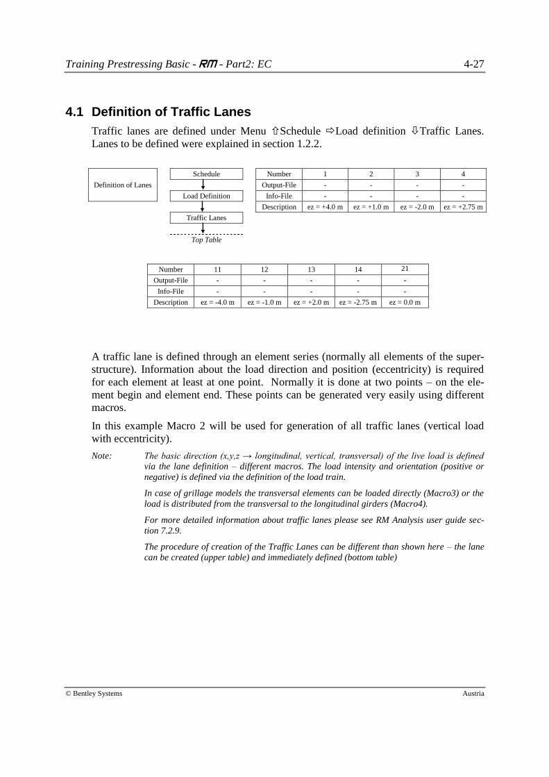
4.1 Definition of Traffic Lanes
Traffic lanes are defined under Menu Schedule Load definition Traffic Lanes.
Lanes to be defined were explained in section 1.2.2.
Definition of Lanes
Schedule Number 1 2 3 4
Output-File - - - -
Load Definition Info-File - - - -
Description ez = +4.0 m ez = +1.0 m ez = -2.0 m ez = +2.75 m
Traffic Lanes
Top Table
Number 11 12 13 14 21
Output-File - - - - -
Info-File - - - - -
Description ez = -4.0 m ez = -1.0 m ez = +2.0 m ez = -2.75 m ez = 0.0 m
A traffic lane is defined through an element series (normally all elements of the super-
structure). Information about the load direction and position (eccentricity) is required
for each element at least at one point. Normally it is done at two points – on the ele-
ment begin and element end. These points can be generated very easily using different
macros.
In this example Macro 2 will be used for generation of all traffic lanes (vertical load
with eccentricity).
Note: The basic direction (x,y,z → longitudinal, vertical, transversal) of the live load is defined
via the lane definition – different macros. The load intensity and orientation (positive or
negative) is defined via the definition of the load train.
In case of grillage models the transversal elements can be loaded directly (Macro3) or the
load is distributed from the transversal to the longitudinal girders (Macro4).
For more detailed information about traffic lanes please see RM Analysis user guide sec-
tion 7.2.9.
The procedure of creation of the Traffic Lanes can be different than shown here – the lane
can be created (upper table) and immediately defined (bottom table)
Training Prestressing Basic - RM - Part2: EC 4-28
© Bentley Systems Austria
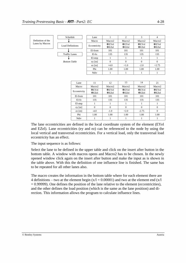
Definition of the
Lanes by Macros
Schedule Lane 1 2 3 4
Macro Macro2 Macro2 Macro2 Macro2
Load Definitions Eccentricity EYel EZel
EYel EZel
EYel EZel
EYel EZel
El-from 101 101 101 101
Traffic Lanes El-fo 135 135 135 135
El-step 1 1 1 1
Bottom Table ey [m] 0 0 0 0
ez [m] +4.0 +1.0 -2.0 +2.75
Phi 1.00 1.00 1.00 1.00
Ndiv 1 1 1 1
Lane 11 12 13 14 21
Macro Macro2 Macro2 Macro2 Macro2 Macro2
Eccentricity EYel
EZel
EYel
EZel
EYel
EZel
EYel
EZel
EYel
EZel
El-from 101 101 101 101 101
El-fo 135 135 135 135 135
El-step 1 1 1 1 1
ey [m] 0 0 0 0 0
ez [m] -4.0 -1.0 +2.0 -2.75 0
Phi 1.00 1.00 1.00 1.00 1.00
Ndiv 1 1 1 1 1
The lane eccentricities are defined in the local coordinate system of the element (EYel
and EZel). Lane eccentricities (ey and ez) can be referenced to the node by using the
local vertical and transversal eccentricities. For a vertical load, only the transversal load
eccentricity has an effect.
The input sequence is as follows:
Select the lane to be defined in the upper table and click on the insert after button in the
bottom table. A window with macros opens and Macro2 has to be chosen. In the newly
opened window click again on the insert after button and make the input as is shown in
the table above. With this the definition of one influence line is finished. The same has
to be repeated for all other lanes also.
The macro creates the information in the bottom table where for each element there are
4 definitions – two at the element begin (x/l = 0.00001) and two at the element end (x/l
= 0.99999). One defines the position of the lane relative to the element (eccentricities),
and the other defines the load position (which is the same as the lane position) and di-
rection. This information allows the program to calculate influence lines.
Training Prestressing Basic - RM - Part2: EC 4-29
© Bentley Systems Austria
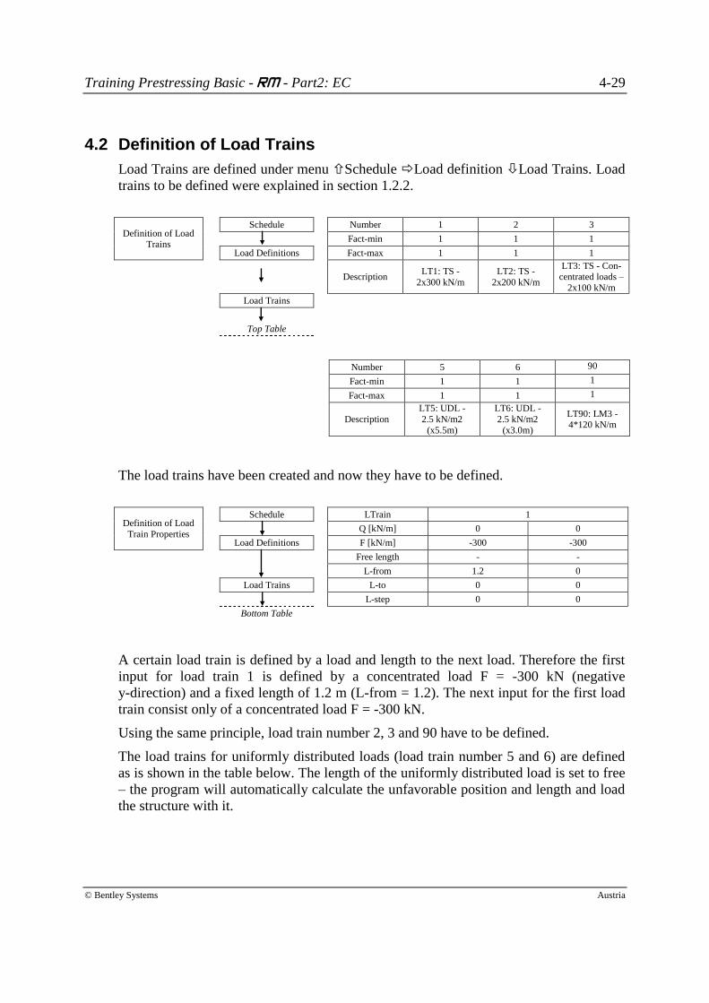
4.2 Definition of Load Trains
Load Trains are defined under menu Schedule Load definition Load Trains. Load
trains to be defined were explained in section 1.2.2.
Definition of Load Trains
Schedule Number 1 2 3
Fact-min 1 1 1
Load Definitions Fact-max 1 1 1
Description LT1: TS -
2x300 kN/m
LT2: TS -
2x200 kN/m
LT3: TS - Con-
centrated loads –
2x100 kN/m
Load Trains
Top Table
Number 5 6 90
Fact-min 1 1 1
Fact-max 1 1 1
Description
LT5: UDL -
2.5 kN/m2
(x5.5m)
LT6: UDL -
2.5 kN/m2
(x3.0m)
LT90: LM3 - 4*120 kN/m
The load trains have been created and now they have to be defined.
Definition of Load
Train Properties
Schedule LTrain 1
Q [kN/m] 0 0
Load Definitions F [kN/m] -300 -300
Free length - -
L-from 1.2 0
Load Trains L-to 0 0
L-step 0 0
Bottom Table
A certain load train is defined by a load and length to the next load. Therefore the first
input for load train 1 is defined by a concentrated load F = -300 kN (negative
y-direction) and a fixed length of 1.2 m (L-from = 1.2). The next input for the first load
train consist only of a concentrated load F = -300 kN.
Using the same principle, load train number 2, 3 and 90 have to be defined.
The load trains for uniformly distributed loads (load train number 5 and 6) are defined
as is shown in the table below. The length of the uniformly distributed load is set to free
– the program will automatically calculate the unfavorable position and length and load
the structure with it.
Training Prestressing Basic - RM - Part2: EC 4-30
© Bentley Systems Austria
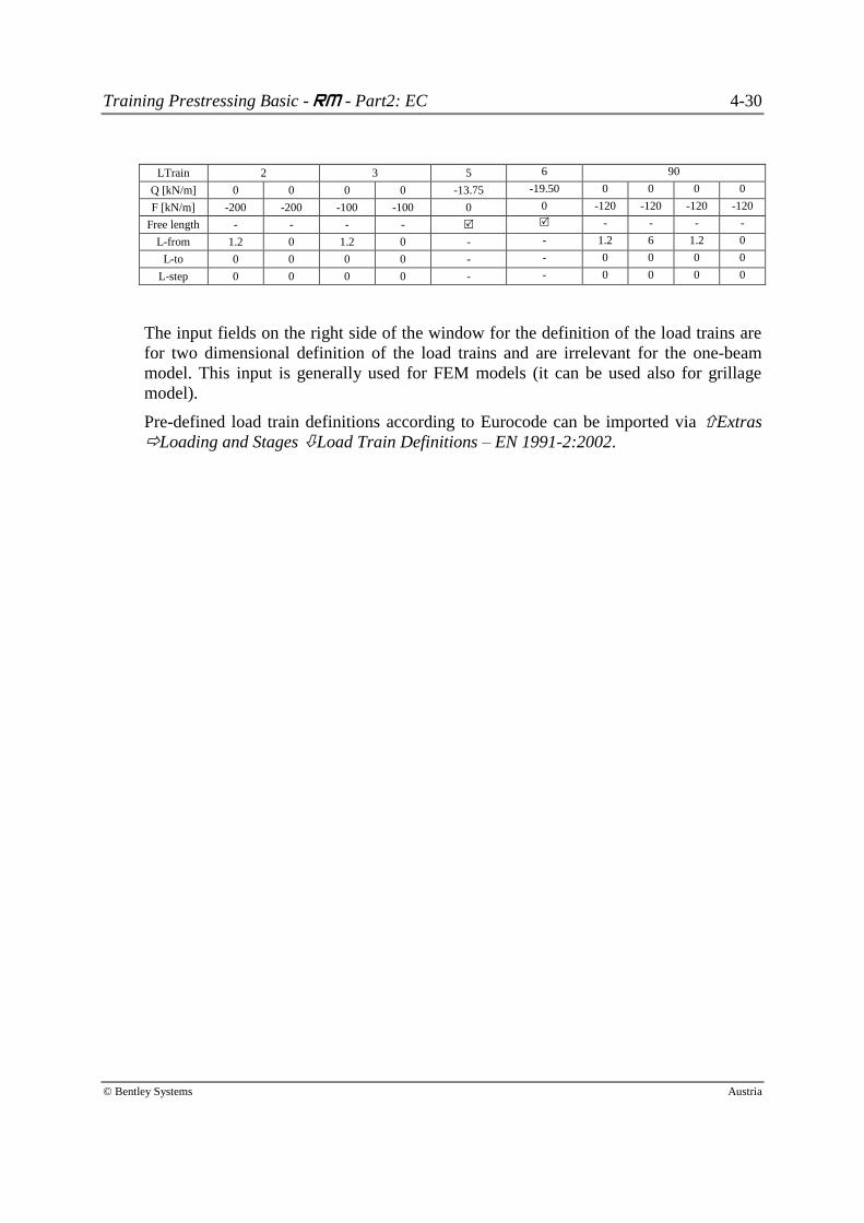
LTrain 2 3 5 6 90
Q [kN/m] 0 0 0 0 -13.75 -19.50 0 0 0 0
F [kN/m] -200 -200 -100 -100 0 0 -120 -120 -120 -120
Free length - - - - - - - -
L-from 1.2 0 1.2 0 - - 1.2 6 1.2 0
L-to 0 0 0 0 - - 0 0 0 0
L-step 0 0 0 0 - - 0 0 0 0
The input fields on the right side of the window for the definition of the load trains are
for two dimensional definition of the load trains and are irrelevant for the one-beam
model. This input is generally used for FEM models (it can be used also for grillage
model).
Pre-defined load train definitions according to Eurocode can be imported via Extras
Loading and Stages Load Train Definitions – EN 1991-2:2002.
Training Prestressing Basic - RM - Part2: EC 4-31
© Bentley Systems Austria
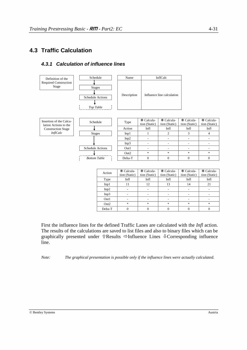
4.3 Traffic Calculation
4.3.1 Calculation of influence lines
Definition of the
Required Construction
Stage
Schedule Name InflCalc
Description Influence line calculation
Stages
Schedule Actions
Top Table
Insertion of the Calcu-lation Actions to the
Construction Stage
InflCalc
Schedule Type Calcula-tion (Static)
Calcula-tion (Static)
Calcula-tion (Static)
Calcula-tion (Static)
Action Infl Infl Infl Infl
Stages Inp1 1 2 3 4
Inp2 - - - -
Inp3 - - - -
Schedule Actions Out1 - - - -
Out2 * * * *
Bottom Table Delta-T 0 0 0 0
Action Calcula-tion (Static)
Calcula-tion (Static)
Calcula-tion (Static)
Calcula-tion (Static)
Calcula-tion (Static)
Type Infl Infl Infl Infl Infl
Inp1 11 12 13 14 21
Inp2 - - - - -
Inp3 - - - - -
Out1 - - - - -
Out2 * * * * *
Delta-T 0 0 0 0 0
First the influence lines for the defined Traffic Lanes are calculated with the Infl action.
The results of the calculations are saved to list files and also to binary files which can be
graphically presented under Results Influence Lines Corresponding influence
line.
Note: The graphical presentation is possible only if the influence lines were actually calculated.
Training Prestressing Basic - RM - Part2: EC 4-32
© Bentley Systems Austria
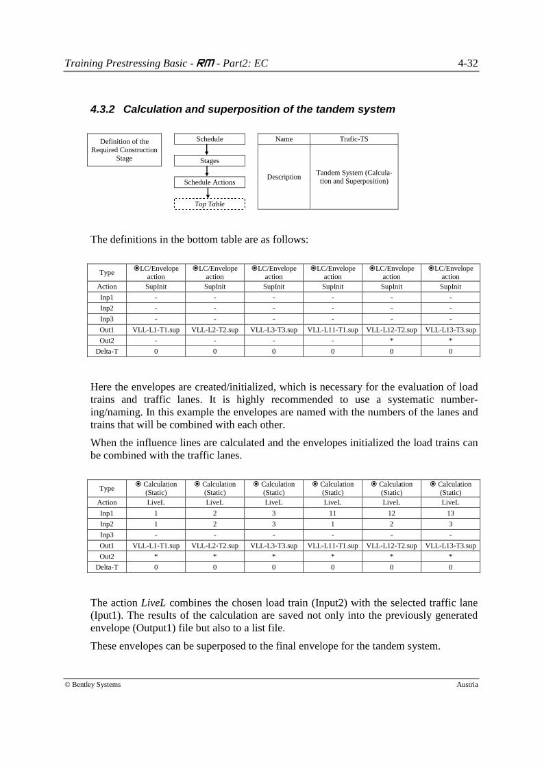
4.3.2 Calculation and superposition of the tandem system
Definition of the
Required Construction
Stage
Schedule Name Trafic-TS
Description Tandem System (Calcula-
tion and Superposition)
Stages
Schedule Actions
Top Table
The definitions in the bottom table are as follows:
Type LC/Envelope
action LC/Envelope
action LC/Envelope
action LC/Envelope
action LC/Envelope
action LC/Envelope
action
Action SupInit SupInit SupInit SupInit SupInit SupInit
Inp1 - - - - - -
Inp2 - - - - - -
Inp3 - - - - - -
Out1 VLL-L1-T1.sup VLL-L2-T2.sup VLL-L3-T3.sup VLL-L11-T1.sup VLL-L12-T2.sup VLL-L13-T3.sup
Out2 - - - - * *
Delta-T 0 0 0 0 0 0
Here the envelopes are created/initialized, which is necessary for the evaluation of load
trains and traffic lanes. It is highly recommended to use a systematic number-
ing/naming. In this example the envelopes are named with the numbers of the lanes and
trains that will be combined with each other.
When the influence lines are calculated and the envelopes initialized the load trains can
be combined with the traffic lanes.
Type Calculation
(Static)
Calculation
(Static)
Calculation
(Static)
Calculation
(Static)
Calculation
(Static)
Calculation
(Static)
Action LiveL LiveL LiveL LiveL LiveL LiveL
Inp1 1 2 3 11 12 13
Inp2 1 2 3 1 2 3
Inp3 - - - - - -
Out1 VLL-L1-T1.sup VLL-L2-T2.sup VLL-L3-T3.sup VLL-L11-T1.sup VLL-L12-T2.sup VLL-L13-T3.sup
Out2 * * * * * *
Delta-T 0 0 0 0 0 0
The action LiveL combines the chosen load train (Input2) with the selected traffic lane
(Iput1). The results of the calculation are saved not only into the previously generated
envelope (Output1) file but also to a list file.
These envelopes can be superposed to the final envelope for the tandem system.
Training Prestressing Basic - RM - Part2: EC 4-33
© Bentley Systems Austria
Type LC/Envelope
action
LC/Envelope
action
LC/Envelope
action
LC/Envelope
action
Action SupInit SupAndSup SupAndSup SupAndSup
Inp1 - LM1-TS-A.sup LM1-TS-A.sup LM1-TS-A.sup
Inp2 - VLL-L1-T1.sup VLL-L2-T2.sup VLL-L3-T3.sup
Inp3 - - - -
Out1 LM1-TS-A.sup - - -
Out2 - - - -
Delta-T 0 0 0 0
Type LC/Envelope
action
LC/Envelope
action
LC/Envelope
action
LC/Envelope
action
Action SupInit SupAndSup SupAndSup SupAndSup
Inp1 - LM1-TS-B.sup LM1-TS-B.sup LM1-TS-B.sup
Inp2 - VLL-L11-T1.sup VLL-L12-T2.sup VLL-L13-T3.sup
Inp3 - - - -
Out1 LM1-TS-B.sup - - -
Out2 - - - -
Delta-T 0 0 0 0
Type LC/Envelope
action
LC/Envelope
action
LC/Envelope
action
Action SupInit SupOrSup SupOrSup
Inp1 - LM1-TS.sup LM1-TS.sup
Inp2 - LM1-TS-A.sup LM1-TS-B.sup
Inp3 - - -
Out1 LM1-TS.sup - -
Out2 - - -
Delta-T 0 0 0
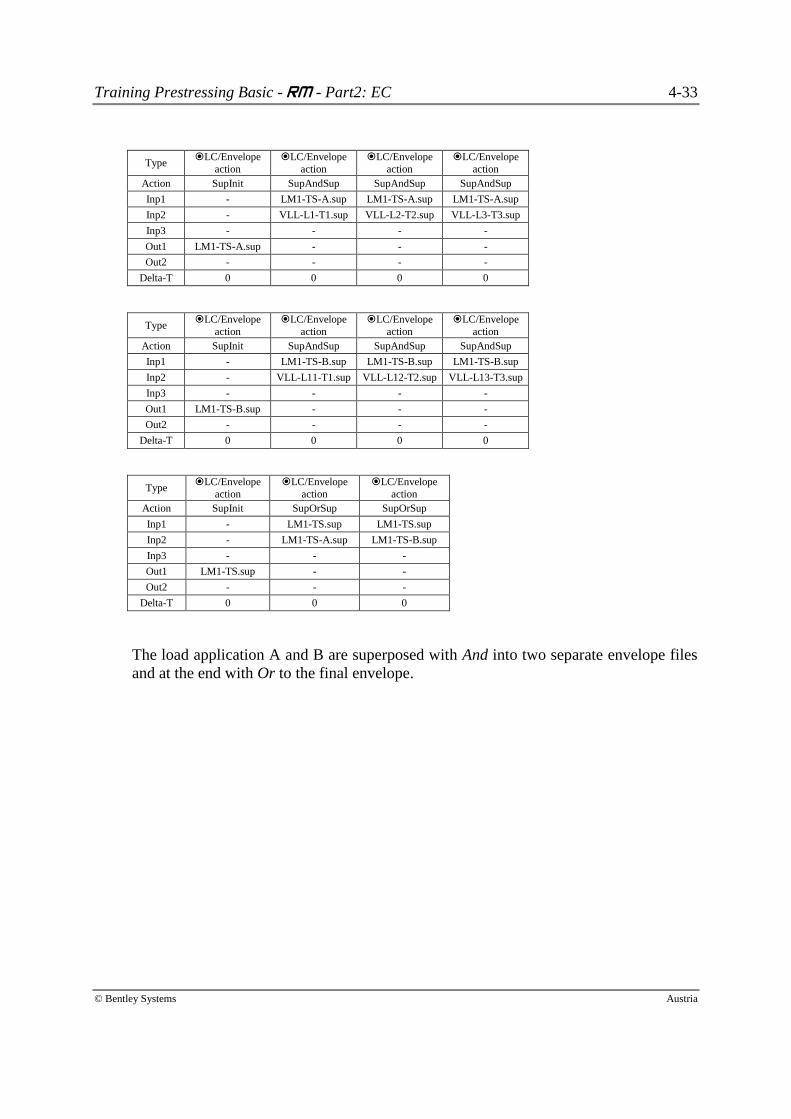
The load application A and B are superposed with And into two separate envelope files
and at the end with Or to the final envelope.
Training Prestressing Basic - RM - Part2: EC 4-34
© Bentley Systems Austria
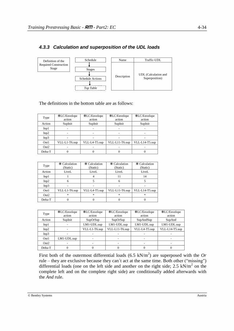
4.3.3 Calculation and superposition of the UDL loads
Definition of the
Required Construction
Stage
Schedule Name Traffic-UDL
Description UDL (Calculation and
Superposition)
Stages
Schedule Actions
Top Table
The definitions in the bottom table are as follows:
Type LC/Envelope
action LC/Envelope
action LC/Envelope
action LC/Envelope
action
Action SupInit SupInit SupInit SupInit
Inp1 - - - -
Inp2 - - - -
Inp3 - - - -
Out1 VLL-L1-T6.sup VLL-L4-T5.sup VLL-L11-T6.sup VLL-L14-T5.sup
Out2 - - - -
Delta-T 0 0 0 0
Type Calculation
(Static)
Calculation
(Static)
Calculation
(Static)
Calculation
(Static)
Action LiveL LiveL LiveL LiveL
Inp1 1 4 11 14
Inp2 6 5 6 5
Inp3 - - - -
Out1 VLL-L1-T6.sup VLL-L4-T5.sup VLL-L11-T6.sup VLL-L14-T5.sup
Out2 * * * *
Delta-T 0 0 0 0
Type LC/Envelope
action
LC/Envelope
action
LC/Envelope
action
LC/Envelope
action
LC/Envelope
action
Action SupInit SupOrSup SupOrSup SupAndSup SupAnd
Inp1 - LM1-UDL.sup LM1-UDL.sup LM1-UDL.sup LM1-UDL.sup
Inp2 - VLL-L1-T6.sup VLL-L11-T6.sup VLL-L4-T5.sup VLL-L14-T5.sup
Inp3 - - - - -
Out1 LM1-UDL.sup - - - -
Out2 - - - - -
Delta-T 0 0 0 0 0
First both of the outermost differential loads (6.5 kN/m2) are superposed with the Or
rule – they are exclusive because they can´t act at the same time. Both other (“missing")
differential loads (one on the left side and another on the right side; 2.5 kN/m2 on the
complete left and on the complete right side) are conditionally added afterwards with
the And rule.
Training Prestressing Basic - RM - Part2: EC 4-35
© Bentley Systems Austria
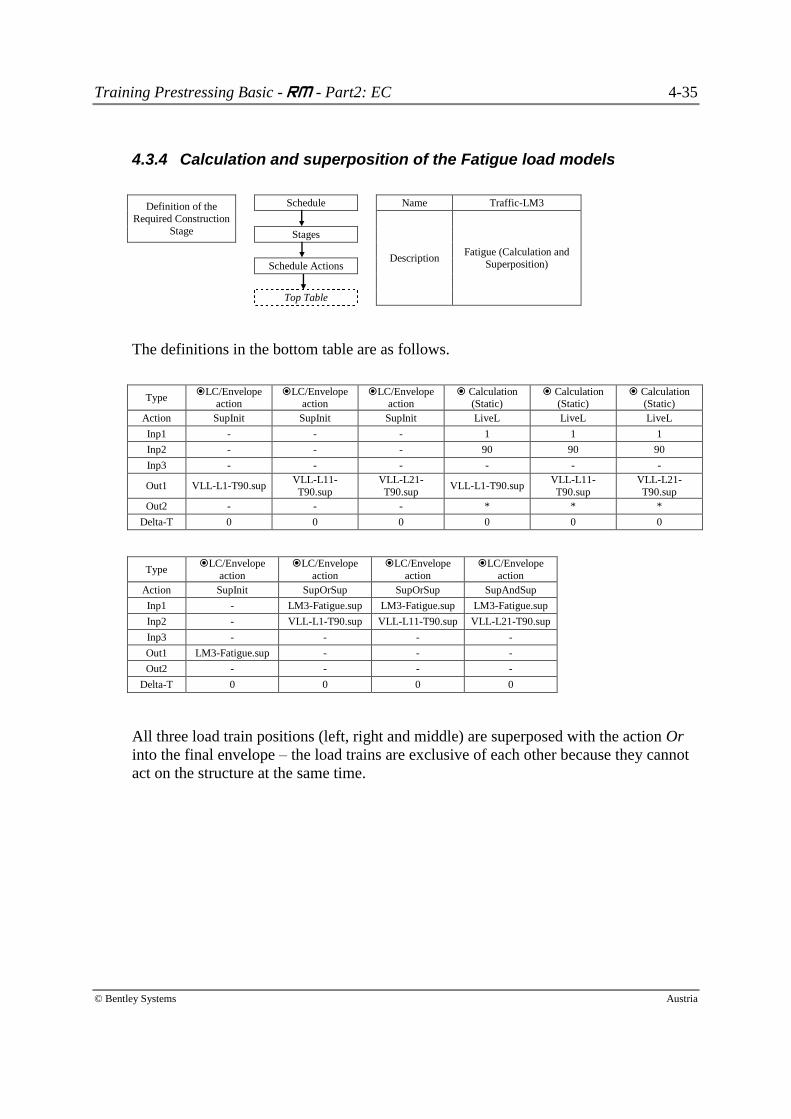
4.3.4 Calculation and superposition of the Fatigue load models
Definition of the
Required Construction
Stage
Schedule Name Traffic-LM3
Description Fatigue (Calculation and
Superposition)
Stages
Schedule Actions
Top Table
The definitions in the bottom table are as follows.
Type LC/Envelope
action LC/Envelope
action LC/Envelope
action Calculation
(Static) Calculation
(Static) Calculation
(Static)
Action SupInit SupInit SupInit LiveL LiveL LiveL
Inp1 - - - 1 1 1
Inp2 - - - 90 90 90
Inp3 - - - - - -
Out1 VLL-L1-T90.sup VLL-L11-
T90.sup
VLL-L21-
T90.sup VLL-L1-T90.sup
VLL-L11-
T90.sup
VLL-L21-
T90.sup
Out2 - - - * * *
Delta-T 0 0 0 0 0 0
Type LC/Envelope
action
LC/Envelope
action
LC/Envelope
action
LC/Envelope
action
Action SupInit SupOrSup SupOrSup SupAndSup
Inp1 - LM3-Fatigue.sup LM3-Fatigue.sup LM3-Fatigue.sup
Inp2 - VLL-L1-T90.sup VLL-L11-T90.sup VLL-L21-T90.sup
Inp3 - - - -
Out1 LM3-Fatigue.sup - - -
Out2 - - - -
Delta-T 0 0 0 0
All three load train positions (left, right and middle) are superposed with the action Or
into the final envelope – the load trains are exclusive of each other because they cannot
act on the structure at the same time.
Training Prestressing Basic - RM - Part2: EC 5-36
© Bentley Systems Austria
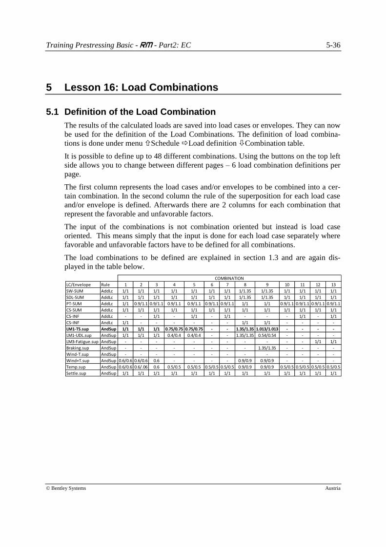
5 Lesson 16: Load Combinations
5.1 Definition of the Load Combination
The results of the calculated loads are saved into load cases or envelopes. They can now
be used for the definition of the Load Combinations. The definition of load combina-
tions is done under menu Schedule Load definition Combination table.
It is possible to define up to 48 different combinations. Using the buttons on the top left
side allows you to change between different pages – 6 load combination definitions per
page.
The first column represents the load cases and/or envelopes to be combined into a cer-
tain combination. In the second column the rule of the superposition for each load case
and/or envelope is defined. Afterwards there are 2 columns for each combination that
represent the favorable and unfavorable factors.
The input of the combinations is not combination oriented but instead is load case
oriented. This means simply that the input is done for each load case separately where
favorable and unfavorable factors have to be defined for all combinations.
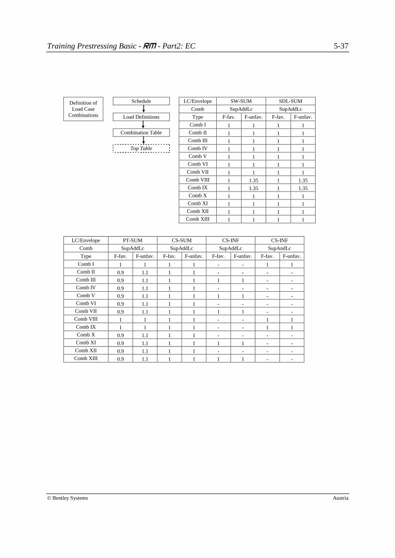
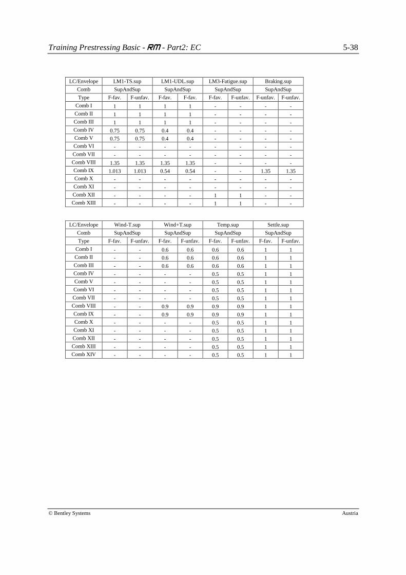
The load combinations to be defined are explained in section 1.3 and are again dis-
played in the table below.
LC/Envelope Rule 1 2 3 4 5 6 7 8 9 10 11 12 13
SW-SUM AddLc 1/1 1/1 1/1 1/1 1/1 1/1 1/1 1/1.35 1/1.35 1/1 1/1 1/1 1/1
SDL-SUM AddLc 1/1 1/1 1/1 1/1 1/1 1/1 1/1 1/1.35 1/1.35 1/1 1/1 1/1 1/1
PT-SUM AddLc 1/1 0.9/1.1 0.9/1.1 0.9/1.1 0.9/1.1 0.9/1.1 0.9/1.1 1/1 1/1 0.9/1.1 0.9/1.1 0.9/1.1 0.9/1.1
CS-SUM AddLc 1/1 1/1 1/1 1/1 1/1 1/1 1/1 1/1 1/1 1/1 1/1 1/1 1/1
CS-INF AddLc - - 1/1 - 1/1 - 1/1 - - - 1/1 - 1/1
CS-INF AndLc 1/1 - - - - - - 1/1 1/1 - - - -
LM1-TS.sup AndSup 1/1 1/1 1/1 0.75/0.75 0.75/0.75 - - 1.35/1.35 1.013/1.013 - - - -
LM1-UDL.sup AndSup 1/1 1/1 1/1 0.4/0.4 0.4/0.4 - - 1.35/1.35 0.54/0.54 - - - -
LM3-Fatigue.sup AndSup - - - - - - - - - - - 1/1 1/1
Braking.sup AndSup - - - - - - - - 1.35/1.35 - - - -
Wind-T.sup AndSup - - - - - - - - - - - - -
Wind+T.sup AndSup 0.6/0.6 0.6/0.6 0.6 - - - - 0.9/0.9 0.9/0.9 - - - -
Temp.sup AndSup 0.6/0.6 0.6/.06 0.6 0.5/0.5 0.5/0.5 0.5/0.5 0.5/0.5 0.9/0.9 0.9/0.9 0.5/0.5 0.5/0.5 0.5/0.5 0.5/0.5
Settle.sup AndSup 1/1 1/1 1/1 1/1 1/1 1/1 1/1 1/1 1/1 1/1 1/1 1/1 1/1
COMBINATION
Training Prestressing Basic - RM - Part2: EC 5-37
© Bentley Systems Austria
Definition of
Load Case
Combinations
Schedule LC/Envelope SW-SUM SDL-SUM
Comb SupAddLc SupAddLc
Load Definitions Type F-fav. F-unfav. F-fav. F-unfav.
Comb I 1 1 1 1
Combination Table Comb II 1 1 1 1
Comb III 1 1 1 1
Top Table Comb IV 1 1 1 1
Comb V 1 1 1 1
Comb VI 1 1 1 1
Comb VII 1 1 1 1
Comb VIII 1 1.35 1 1.35
Comb IX 1 1.35 1 1.35
Comb X 1 1 1 1
Comb XI 1 1 1 1
Comb XII 1 1 1 1
Comb XIII 1 1 1 1
LC/Envelope PT-SUM CS-SUM CS-INF CS-INF
Comb SupAddLc SupAddLc SupAddLc SupAndLc
Type F-fav. F-unfav. F-fav. F-unfav. F-fav. F-unfav. F-fav. F-unfav.
Comb I 1 1 1 1 - - 1 1
Comb II 0.9 1.1 1 1 - - - -
Comb III 0.9 1.1 1 1 1 1 - -
Comb IV 0.9 1.1 1 1 - - - -
Comb V 0.9 1.1 1 1 1 1 - -
Comb VI 0.9 1.1 1 1 - - - -
Comb VII 0.9 1.1 1 1 1 1 - -
Comb VIII 1 1 1 1 - - 1 1
Comb IX 1 1 1 1 - - 1 1
Comb X 0.9 1.1 1 1 - - - -
Comb XI 0.9 1.1 1 1 1 1 - -
Comb XII 0.9 1.1 1 1 - - - -
Comb XIII 0.9 1.1 1 1 1 1 - -
Training Prestressing Basic - RM - Part2: EC 5-38
© Bentley Systems Austria
LC/Envelope LM1-TS.sup LM1-UDL.sup LM3-Fatigue.sup Braking.sup
Comb SupAndSup SupAndSup SupAndSup SupAndSup
Type F-fav. F-unfav. F-fav. F-fav. F-fav. F-unfav. F-unfav. F-unfav.
Comb I 1 1 1 1 - - - -
Comb II 1 1 1 1 - - - -
Comb III 1 1 1 1 - - - -
Comb IV 0.75 0.75 0.4 0.4 - - - -
Comb V 0.75 0.75 0.4 0.4 - - - -
Comb VI - - - - - - - -
Comb VII - - - - - - - -
Comb VIII 1.35 1.35 1.35 1.35 - - - -
Comb IX 1.013 1.013 0.54 0.54 - - 1.35 1.35
Comb X - - - - - - - -
Comb XI - - - - - - - -
Comb XII - - - - 1 1 - -
Comb XIII - - - - 1 1 - -
LC/Envelope Wind-T.sup Wind+T.sup Temp.sup Settle.sup
Comb SupAndSup SupAndSup SupAndSup SupAndSup
Type F-fav. F-unfav. F-fav. F-unfav. F-fav. F-unfav. F-fav. F-unfav.
Comb I - - 0.6 0.6 0.6 0.6 1 1
Comb II - - 0.6 0.6 0.6 0.6 1 1
Comb III - - 0.6 0.6 0.6 0.6 1 1
Comb IV - - - - 0.5 0.5 1 1
Comb V - - - - 0.5 0.5 1 1
Comb VI - - - - 0.5 0.5 1 1
Comb VII - - - - 0.5 0.5 1 1
Comb VIII - - 0.9 0.9 0.9 0.9 1 1
Comb IX - - 0.9 0.9 0.9 0.9 1 1
Comb X - - - - 0.5 0.5 1 1
Comb XI - - - - 0.5 0.5 1 1
Comb XII - - - - 0.5 0.5 1 1
Comb XIII - - - - 0.5 0.5 1 1
Comb XIV - - - - 0.5 0.5 1 1
Training Prestressing Basic - RM - Part2: EC 5-39
© Bentley Systems Austria
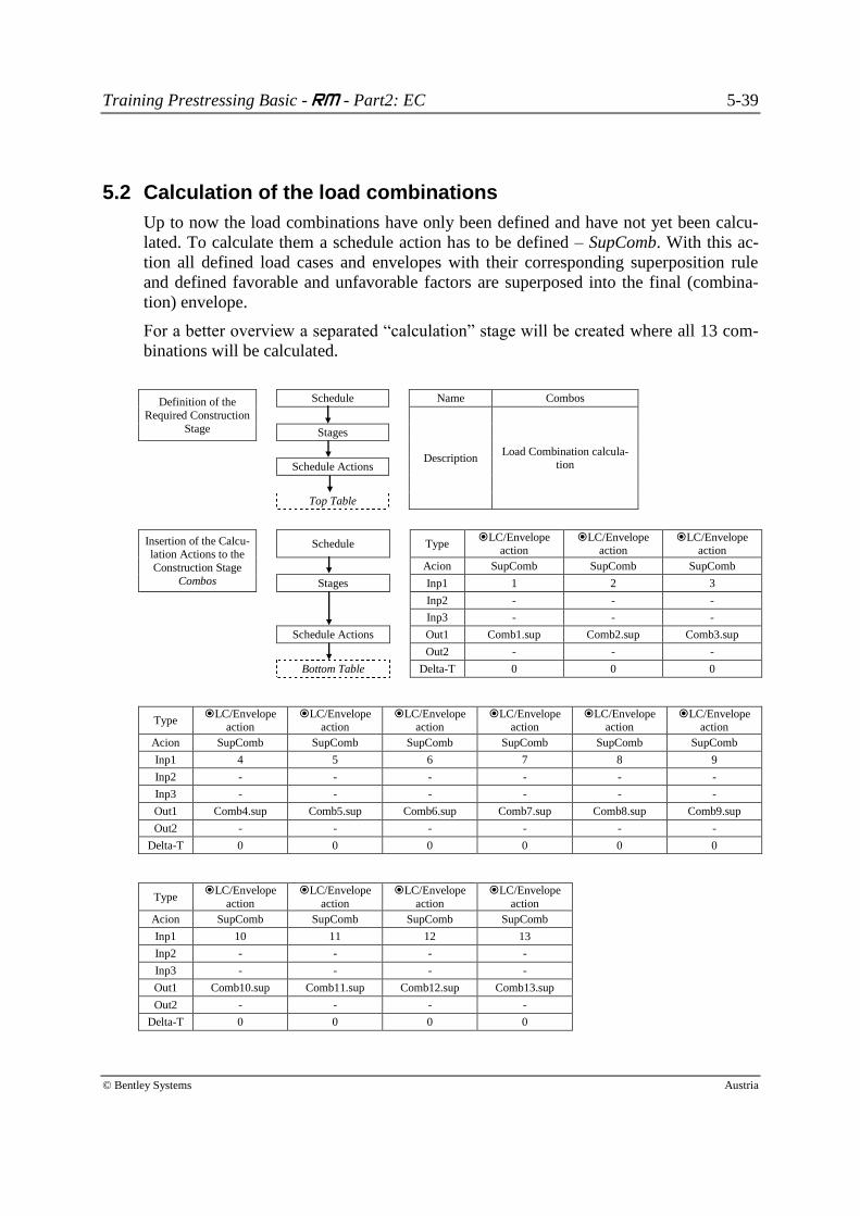
5.2 Calculation of the load combinations
Up to now the load combinations have only been defined and have not yet been calcu-
lated. To calculate them a schedule action has to be defined – SupComb. With this ac-
tion all defined load cases and envelopes with their corresponding superposition rule
and defined favorable and unfavorable factors are superposed into the final (combina-
tion) envelope.
For a better overview a separated “calculation” stage will be created where all 13 com-
binations will be calculated.
Definition of the
Required Construction
Stage
Schedule Name Combos
Description Load Combination calcula-
tion
Stages
Schedule Actions
Top Table
Insertion of the Calcu-lation Actions to the
Construction Stage
Combos
Schedule Type LC/Envelope
action LC/Envelope
action LC/Envelope
action
Acion SupComb SupComb SupComb
Stages Inp1 1 2 3
Inp2 - - -
Inp3 - - -
Schedule Actions Out1 Comb1.sup Comb2.sup Comb3.sup
Out2 - - -
Bottom Table Delta-T 0 0 0
Type LC/Envelope
action LC/Envelope
action LC/Envelope
action LC/Envelope
action LC/Envelope
action LC/Envelope
action
Acion SupComb SupComb SupComb SupComb SupComb SupComb
Inp1 4 5 6 7 8 9
Inp2 - - - - - -
Inp3 - - - - - -
Out1 Comb4.sup Comb5.sup Comb6.sup Comb7.sup Comb8.sup Comb9.sup
Out2 - - - - - -
Delta-T 0 0 0 0 0 0
Type LC/Envelope
action
LC/Envelope
action
LC/Envelope
action
LC/Envelope
action
Acion SupComb SupComb SupComb SupComb
Inp1 10 11 12 13
Inp2 - - - -
Inp3 - - - -
Out1 Comb10.sup Comb11.sup Comb12.sup Comb13.sup
Out2 - - - -
Delta-T 0 0 0 0
Training Prestressing Basic - RM - Part2: EC 6-40
© Bentley Systems Austria
6 Lesson 17: Fibre Stress Check
Definition of the
Required Construc-
tion Stage
Schedule Name SLS
Description
SLS-Fibre Stress
Check - Concrete compression stresses
and decompression
Stages
Activation
Top Table
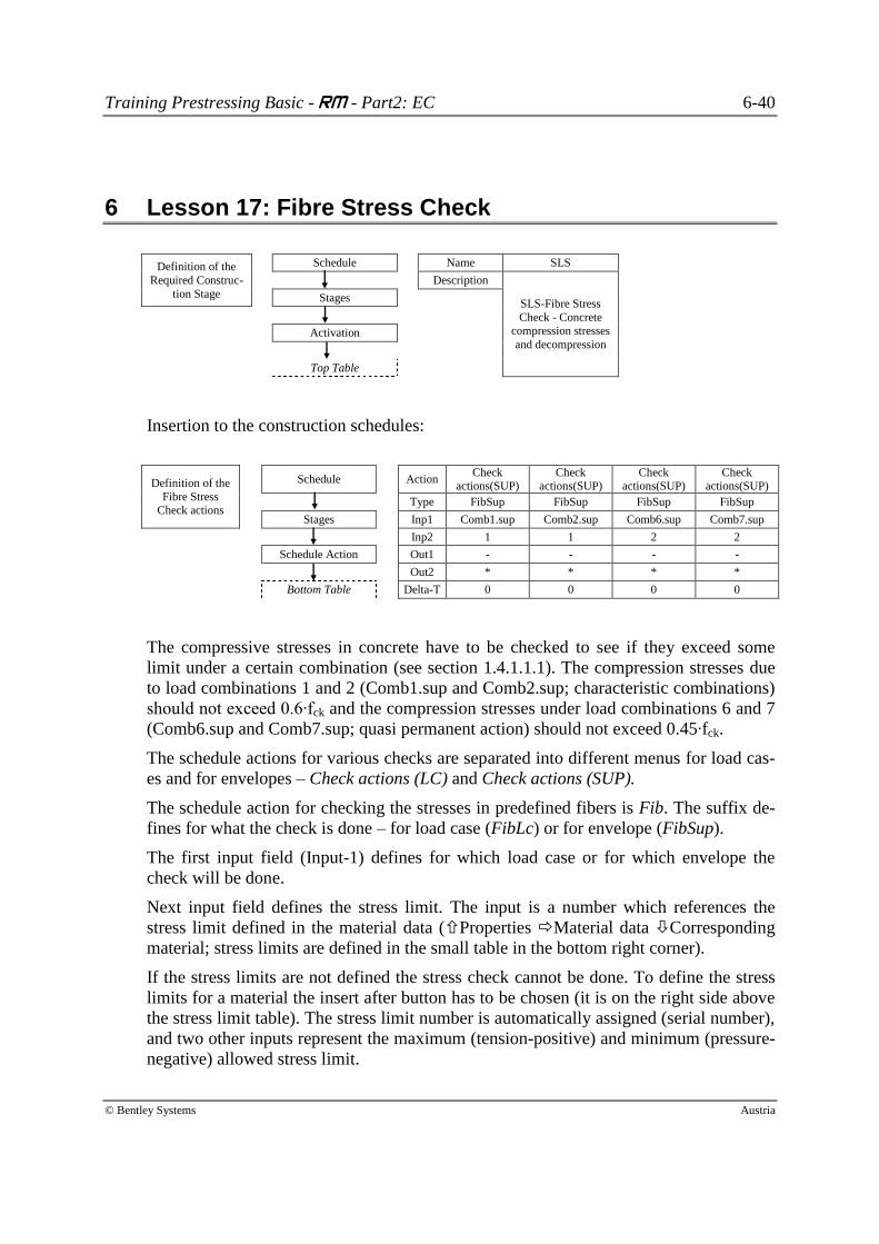
Insertion to the construction schedules:
Definition of the
Fibre Stress Check actions
Schedule Action Check
actions(SUP) Check
actions(SUP) Check
actions(SUP) Check
actions(SUP)
Type FibSup FibSup FibSup FibSup
Stages Inp1 Comb1.sup Comb2.sup Comb6.sup Comb7.sup
Inp2 1 1 2 2
Schedule Action Out1 - - - -
Out2 * * * *
Bottom Table Delta-T 0 0 0 0
The compressive stresses in concrete have to be checked to see if they exceed some
limit under a certain combination (see section 1.4.1.1.1). The compression stresses due
to load combinations 1 and 2 (Comb1.sup and Comb2.sup; characteristic combinations)
should not exceed 0.6∙fck and the compression stresses under load combinations 6 and 7
(Comb6.sup and Comb7.sup; quasi permanent action) should not exceed 0.45∙fck.
The schedule actions for various checks are separated into different menus for load cas-
es and for envelopes – Check actions (LC) and Check actions (SUP).
The schedule action for checking the stresses in predefined fibers is Fib. The suffix de-
fines for what the check is done – for load case (FibLc) or for envelope (FibSup).
The first input field (Input-1) defines for which load case or for which envelope the
check will be done.
Next input field defines the stress limit. The input is a number which references the
stress limit defined in the material data (Properties Material data Corresponding
material; stress limits are defined in the small table in the bottom right corner).
If the stress limits are not defined the stress check cannot be done. To define the stress
limits for a material the insert after button has to be chosen (it is on the right side above
the stress limit table). The stress limit number is automatically assigned (serial number),
and two other inputs represent the maximum (tension-positive) and minimum (pressure-
negative) allowed stress limit.
Training Prestressing Basic - RM - Part2: EC 6-41
© Bentley Systems Austria
In this case the stress limits are already defined. The stress limit number 1 corresponds
to 0.6∙fck, and the stress limit number 2 corresponds to 0.45∙fck.
The check determines the minimum and maximum stresses under the defined load
case/envelope in all stress check points defined in the cross-sections and compares them
with stress limits. Results are saved into a list file (Output-2). Those exceeding the lim-
its (if there are any) are saved into the list file (values marked with #), and a warning is
displayed after completion of the calculation.
The same check can also be done graphically. It can be seen at which places the re-
quirements are not satisfied. This is done by creating a diagram via RMSet. On this dia-
gram certain stresses in certain fibers are plotted along with stress limits.
Training Prestressing Basic - RM - Part2: EC 7-42
© Bentley Systems Austria
7 Reinforced concrete checks – General
The results of different design check actions are reinforcement areas that are saved into
their corresponding Attribute-Sets. They can be seen under menu Structure Ele-
ments Checks for each element.
In the upper table the element is selected and in the bottom table the results can be seen
by selecting one of the corresponding Attribute Set.
Some Attribute Sets have more than one result component (e.g.: Attribute Set for Shear-
Longitudinal reinforcement which has two result components – one for the top and
another for the bottom reinforcement).
The calculated reinforcement areas are stored and displayed under the A2 reinforcement
area. The A1 reinforcement area represents an input where a predefined reinforcement
area (e.g.: minimum reinforcement) can be defined (double click on the Attribute Set or
select it and click on the modify button). It is possible to define that this reinforcement
area is fixed or variable. If it is set to fixed, then the program will not increase the val-
ues even if it is necessary according to a certain design check. In the other case the rein-
forcement area will be increased by the necessary reinforcement area calculated by a
certain design check.
The reinforcement areas can be displayed also graphically via RM-Sets. The corres-
ponding elements and attribute sets have to be defined. In addition the results can be
presented numerically by creating an excel sheet or a list file.
It is also possible to specify for which elements certain design checks should not be
done (double click on an element in the upper table and check the OFF button next to a
certain design check). By default all design checks are ON for all elements. The pro-
gram distinguishes between beam elements and other elements (spring elements, stiff-
ness elements, tendons, etc.). In addition it is also possible to make a detailed list file
(export) for each design check.
In principal the reinforcement area calculated by previous design actions (depending on
the schedule sequence defined in under schedule actions) is taken into account in the
subsequent design actions.
The data of the calculated reinforcement area (A2) remains as an existing reinforcement
area even when a new recalculation of the project is run (it is also exported into TCL
files). Therefore it is necessary to initialize (delete) the A2 reinforcement areas (calcu-
lated areas) before the first design action. This is done with the ReinIni action (Rein-
forcement Initialization) where the A2 reinforcement area of a certain or all Attribute
sets is set to 0 for all elements.
Training Prestressing Basic - RM - Part2: EC 7-43
© Bentley Systems Austria
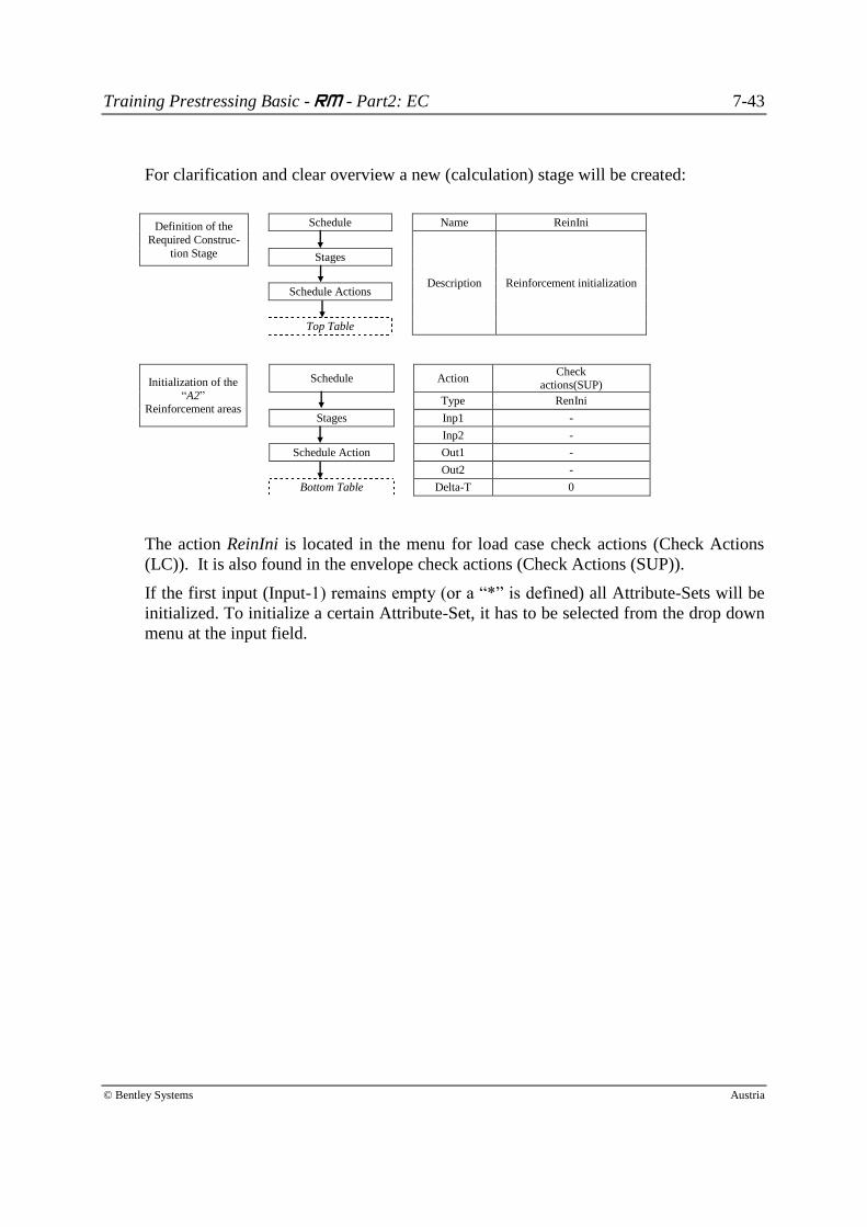
For clarification and clear overview a new (calculation) stage will be created:
Definition of the
Required Construc-
tion Stage
Schedule Name ReinIni
Description Reinforcement initialization
Stages
Schedule Actions
Top Table
Initialization of the
“A2” Reinforcement areas
Schedule Action Check
actions(SUP)
Type RenIni
Stages Inp1 -
Inp2 -
Schedule Action Out1 -
Out2 -
Bottom Table Delta-T 0
The action ReinIni is located in the menu for load case check actions (Check Actions
(LC)). It is also found in the envelope check actions (Check Actions (SUP)).
If the first input (Input-1) remains empty (or a “*” is defined) all Attribute-Sets will be
initialized. To initialize a certain Attribute-Set, it has to be selected from the drop down
menu at the input field.
Training Prestressing Basic - RM - Part2: EC 8-44
© Bentley Systems Austria
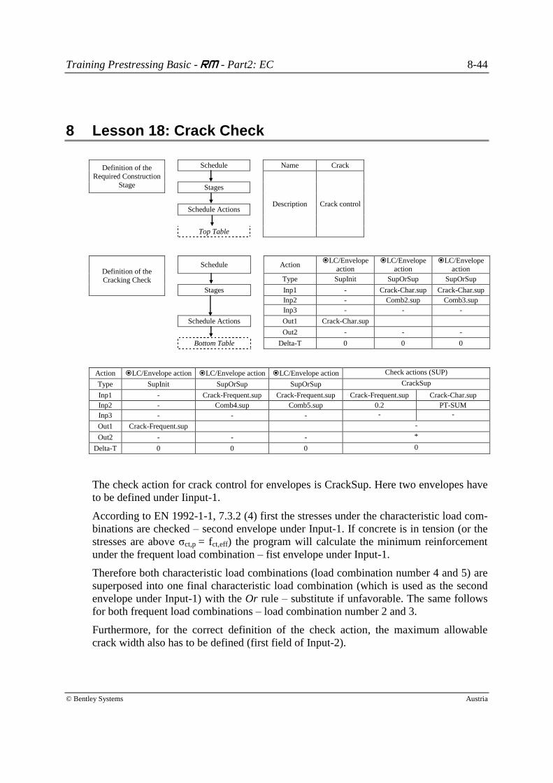
8 Lesson 18: Crack Check
Definition of the
Required Construction
Stage
Schedule Name Crack
Description Crack control
Stages
Schedule Actions
Top Table
Definition of the
Cracking Check
Schedule Action LC/Envelope
action LC/Envelope
action LC/Envelope
action
Type SupInit SupOrSup SupOrSup
Stages Inp1 - Crack-Char.sup Crack-Char.sup
Inp2 - Comb2.sup Comb3.sup
Inp3 - - -
Schedule Actions Out1 Crack-Char.sup
Out2 - - -
Bottom Table Delta-T 0 0 0
Action LC/Envelope action LC/Envelope action LC/Envelope action Check actions (SUP)
Type SupInit SupOrSup SupOrSup CrackSup
Inp1 - Crack-Frequent.sup Crack-Frequent.sup Crack-Frequent.sup Crack-Char.sup
Inp2 - Comb4.sup Comb5.sup 0.2 PT-SUM
Inp3 - - - - -
Out1 Crack-Frequent.sup -
Out2 - - - *
Delta-T 0 0 0 0
The check action for crack control for envelopes is CrackSup. Here two envelopes have
to be defined under Iinput-1.
According to EN 1992-1-1, 7.3.2 (4) first the stresses under the characteristic load com-
binations are checked – second envelope under Input-1. If concrete is in tension (or the
stresses are above σct,p = fct,eff) the program will calculate the minimum reinforcement
under the frequent load combination – fist envelope under Input-1.
Therefore both characteristic load combinations (load combination number 4 and 5) are
superposed into one final characteristic load combination (which is used as the second
envelope under Input-1) with the Or rule – substitute if unfavorable. The same follows
for both frequent load combinations – load combination number 2 and 3.
Furthermore, for the correct definition of the check action, the maximum allowable
crack width also has to be defined (first field of Input-2).
Training Prestressing Basic - RM - Part2: EC 8-45
© Bentley Systems Austria
The last necessary input for the check action is the Initial-strain load case (for more in-
formation see section 9 because the crack check is based on the ultimate load check).
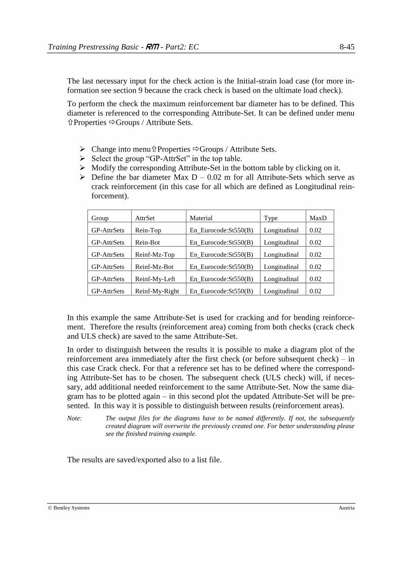
To perform the check the maximum reinforcement bar diameter has to be defined. This
diameter is referenced to the corresponding Attribute-Set. It can be defined under menu
Properties Groups / Attribute Sets.
Change into menuProperties Groups / Attribute Sets.
Select the group “GP-AttrSet” in the top table.
Modify the corresponding Attribute-Set in the bottom table by clicking on it.
Define the bar diameter Max D – 0.02 m for all Attribute-Sets which serve as
crack reinforcement (in this case for all which are defined as Longitudinal rein-
forcement).
Group AttrSet Material Type MaxD
GP-AttrSets Rein-Top En_Eurocode:St550(B) Longitudinal 0.02
GP-AttrSets Rein-Bot En_Eurocode:St550(B) Longitudinal 0.02
GP-AttrSets Reinf-Mz-Top En_Eurocode:St550(B) Longitudinal 0.02
GP-AttrSets Reinf-Mz-Bot En_Eurocode:St550(B) Longitudinal 0.02
GP-AttrSets Reinf-My-Left En_Eurocode:St550(B) Longitudinal 0.02
GP-AttrSets Reinf-My-Right En_Eurocode:St550(B) Longitudinal 0.02
In this example the same Attribute-Set is used for cracking and for bending reinforce-
ment. Therefore the results (reinforcement area) coming from both checks (crack check
and ULS check) are saved to the same Attribute-Set.
In order to distinguish between the results it is possible to make a diagram plot of the
reinforcement area immediately after the first check (or before subsequent check) – in
this case Crack check. For that a reference set has to be defined where the correspond-
ing Attribute-Set has to be chosen. The subsequent check (ULS check) will, if neces-
sary, add additional needed reinforcement to the same Attribute-Set. Now the same dia-
gram has to be plotted again – in this second plot the updated Attribute-Set will be pre-
sented. In this way it is possible to distinguish between results (reinforcement areas).
Note: The output files for the diagrams have to be named differently. If not, the subsequently
created diagram will overwrite the previously created one. For better understanding please
see the finished training example.
The results are saved/exported also to a list file.
Training Prestressing Basic - RM - Part2: EC 9-46
© Bentley Systems Austria
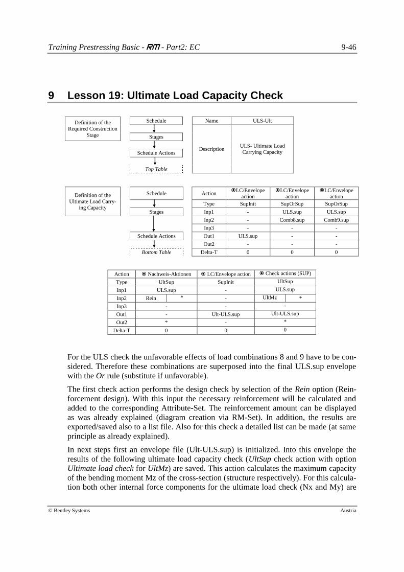
9 Lesson 19: Ultimate Load Capacity Check
Definition of the
Required Construction
Stage
Schedule Name ULS-Ult
Description ULS- Ultimate Load Carrying Capacity
Stages
Schedule Actions
Top Table
Definition of the
Ultimate Load Carry-ing Capacity
Schedule Action LC/Envelope
action LC/Envelope
action LC/Envelope
action
Type SupInit SupOrSup SupOrSup
Stages Inp1 - ULS.sup ULS.sup
Inp2 - Comb8.sup Comb9.sup
Inp3 - - -
Schedule Actions Out1 ULS.sup - -
Out2 - - -
Bottom Table Delta-T 0 0 0
Action Nachweis-Aktionen LC/Envelope action Check actions (SUP)
Type UltSup SupInit UltSup
Inp1 ULS.sup - ULS.sup
Inp2 Rein * - UltMz *
Inp3 - - -
Out1 - Ult-ULS.sup Ult-ULS.sup
Out2 * - *
Delta-T 0 0 0
For the ULS check the unfavorable effects of load combinations 8 and 9 have to be con-
sidered. Therefore these combinations are superposed into the final ULS.sup envelope
with the Or rule (substitute if unfavorable).
The first check action performs the design check by selection of the Rein option (Rein-
forcement design). With this input the necessary reinforcement will be calculated and
added to the corresponding Attribute-Set. The reinforcement amount can be displayed
as was already explained (diagram creation via RM-Set). In addition, the results are
exported/saved also to a list file. Also for this check a detailed list can be made (at same
principle as already explained).
In next steps first an envelope file (Ult-ULS.sup) is initialized. Into this envelope the
results of the following ultimate load capacity check (UltSup check action with option
Ultimate load check for UltMz) are saved. This action calculates the maximum capacity
of the bending moment Mz of the cross-section (structure respectively). For this calcula-
tion both other internal force components for the ultimate load check (Nx and My) are
Training Prestressing Basic - RM - Part2: EC 9-47
© Bentley Systems Austria
fixed, and only the bending moment Mz is increased until the maximum capacity of the
bending moment is reached. The iteration process varies the strain planes which are
based on the stress-strain diagram of the corresponding element (concrete, reinforce-
ment steel and pre-stressing steel). These diagrams are defined under material proper-
ties. Also these results are saved to a list file.
For pre-stressed structures the initial strain load case has to be defined to correctly con-
sider the initial strain of the pre-stressing steel caused by the primary state of pre-
stressing (V*e) when evaluating the stress-strain diagram. This state is saved in the
summation load case of pre-stressing (PT-SUM).
To consider the initial strain of creep and shrinkage and relaxation also, the total sum-
mation load case (STG-SUM) should be defined as the initial strain load case.
Furthermore, it is possible to consider the initial strain state from the envelope (load
case respectively) used for the design check. To do so, a “*” has to be defined, instead
of certain load case in the corresponding input field. This option considers also the fac-
tored initial strain of time effects. However, this is not allowed if the envelope includes
factored pre-stressing load cases and time effects and is not relevant in this form for
consideration of initial strain (see combination factors for combination used for crack
check).
If no initial strain load case is defined, then the load case defined in the recalc pad is
used as initial strain load case. If no load case is defined in the recalc pad, then the ini-
tial strain is not considered.
For more information about the ultimate load check and design of reinforced concrete
with or without pre-stressing see RM Analysis User Guide section 15.3 and 15.4.
A very instructive graphical comparison between demand moments (ULS.sup) and ul-
timate moments (Ult-SUL.sup) is done in the corresponding example.
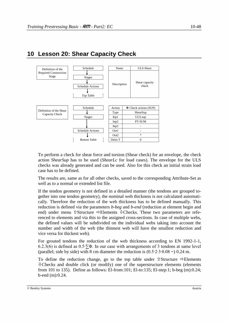
Training Prestressing Basic - RM - Part2: EC 10-48
© Bentley Systems Austria
10 Lesson 20: Shear Capacity Check
Definition of the
Required Construction
Stage
Schedule Name ULS-Shear
Description Shear capacity
check
Stages
Schedule Actions
Top Table
Definition of the Shear
Capacity Check
Schedule Action Check actions (SUP)
Type ShearSup
Stages Inp1 ULS.sup
Inp2 PT-SUM
Inp3 -
Schedule Actions Out1 -
Out2 *
Bottom Table Delta-T 0
To perform a check for shear force and torsion (Shear check) for an envelope, the check
action ShearSup has to be used (ShearLc for load cases). The envelope for the ULS
checks was already generated and can be used. Also for this check an initial strain load
case has to be defined.
The results are, same as for all other checks, saved to the corresponding Attribute-Set as
well as to a normal or extended list file.
If the tendon geometry is not defined in a detailed manner (the tendons are grouped to-
gether into one tendon geometry), the nominal web thickness is not calculated automati-
cally. Therefore the reduction of the web thickness has to be defined manually. This
reduction is defined via the parameters b-beg and b-end (reduction at element begin and
end) under menu Structure Elements Checks. These two parameters are refe-
renced to elements and via this to the assigned cross-sections. In case of multiple webs,
the defined values will be subdivided on the individual webs taking into account the
number and width of the web (the thinnest web will have the smallest reduction and
vice versa for thickest web).
For grouted tendons the reduction of the web thickness according to EN 1992-1-1,
6.2.3(6) is defined as 0.5∙∑Φ. In our case with arrangements of 3 tendons at same level
(parallel; side by side) with 8 cm diameter the reduction is (0.5∙2∙3∙0.08 =) 0.24 m.
To define the reduction change, go to the top table under Structure Elements
Checks and double click (or modify) one of the superstructure elements (elements
from 101 to 135). Define as follows: El-from:101; El-to:135; El-step:1; b-beg (m):0.24;
b-end (m):0.24.
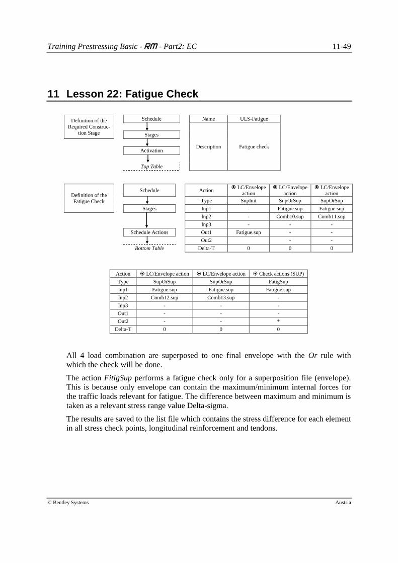
Training Prestressing Basic - RM - Part2: EC 11-49
© Bentley Systems Austria
11 Lesson 22: Fatigue Check
Definition of the
Required Construc-
tion Stage
Schedule Name ULS-Fatigue
Description Fatigue check
Stages
Activation
Top Table
Definition of the
Fatigue Check
Schedule Action LC/Envelope
action LC/Envelope
action LC/Envelope
action
Type SupInit SupOrSup SupOrSup
Stages Inp1 - Fatigue.sup Fatigue.sup
Inp2 - Comb10.sup Comb11.sup
Inp3 - - -
Schedule Actions Out1 Fatigue.sup - -
Out2 - -
Bottom Table Delta-T 0 0 0
Action LC/Envelope action LC/Envelope action Check actions (SUP)
Type SupOrSup SupOrSup FatigSup
Inp1 Fatigue.sup Fatigue.sup Fatigue.sup
Inp2 Comb12.sup Comb13.sup -
Inp3 - - -
Out1 - - -
Out2 - - *
Delta-T 0 0 0
All 4 load combination are superposed to one final envelope with the Or rule with
which the check will be done.
The action FitigSup performs a fatigue check only for a superposition file (envelope).
This is because only envelope can contain the maximum/minimum internal forces for
the traffic loads relevant for fatigue. The difference between maximum and minimum is
taken as a relevant stress range value Delta-sigma.
The results are saved to the list file which contains the stress difference for each element
in all stress check points, longitudinal reinforcement and tendons.
Training Prestressing Basic - RM - Part2: EC 12-50
© Bentley Systems Austria
12 Lesson 23: Lists and Plots
The different possibilities of post processing (RM-Sets and Plot Conatiners) were
shown already in section 11 of Part1. In the corresponding example there are multiple
Rm-Sets and Plots for presentation of internal forces, stresses and reinforcement areas
defined and created/plotted in schedule actions. This definition can be seen directly in
the program.
In addition a new stage is created (last stage) in which additional predefined plot actions
(Schedule Stages Schedule actins; Bottom table → List/Plot actions) are defined
for plotting: working diagrams, creep and shrinkage diagrams, cross-sections, tendon
geometry, tendon scheme, tendon positions in cross-sections, stressing actions, load
trains, influence lines, etc. Also these definitions can be seen directly in the program.
Related Documents