Risk Sharing with Collar Options in Infrastructure Investments · Risk Sharing with Collar Options in Infrastructure Investments Roger Adkins* Bradford University School of Management

Risk Sharing with Collar Options in Infrastructure Investments

Roger Adkins*

Bradford University School of Management

Dean Paxson**

Alliance Manchester Business School

Submitted to the ROC Boston

20 January 2017

Acknowledgements: We thank Alcino Azevedo, Carlos Bastian-Pinto, Graham Davis, Michael

Flanagan, Paulo Pereira, Artur Rodrigues, Anne Stafford, Pam Stapleton, and Luiz Brandão

for helpful comments on earlier versions.

*Bradford University School of Management, Emm Lane, Bradford BD9 4JL, UK.

[email protected]

+44 (0)1274233466.

**Alliance Manchester Business School, Booth St West, Manchester, M15 6PB, UK.

[email protected]

+44(0)1612756353.

2

Risk Sharing with Collar Options in Infrastructure Investments Abstract

A real option model is formulated for infrastructure investments with collars, which are devised

to guarantee a floor cash flow for an active real asset while capping any abnormally high cash

flows. Composed of pairs of put and call American perpetuity options, feasible collars perform

a similar role as investment subsidies by yielding a lower investment threshold, thereby

inducing an earlier exercise than the without-collar variant. While the investment threshold for

the with-collar model is governed only by the floor, the investment option value is influenced

positively by the floor but negatively by the cap, so by appropriately adjusting the floor and

cap, the with-collar investment option value can be engineered to equal that for the without-

collar variant, making it effectively “costless”. A volatility increase makes the with-collar

variant less valuable due to the greater chance of hitting the cap. The “profits” of the

concessionaire are compared to those of the concession granting government under collar, and

floor or ceiling only, viewing the arrangement as a real option game between principal and

agent. The collar analysis is extended to two more complex collar designs, and also compared

with floor only and ceiling only arrangements.

JEL Classifications: D81, G31, H25

Keywords: Decision Analysis, Collar Options, Revenue Floors and Ceilings, Infrastructure

3

1 Introduction

We present a collar option as a suitable policy device for a government (GOV) granting a

concession to induce Public-Private Partnership (PPP) infrastructure investment by a

concessionaire (CON) by guaranteeing a floor in the face of adverse circumstances, and

simultaneously capturing abnormally high returns when the circumstances are sufficiently

favourable. Implementing a collar results in an earlier exercise than for an investment

opportunity without a collar due to the guarantee, while its cost may be partially recouped from

significantly high profits. The analysis of collars adopts a real option formulation because the

guarantee on the downside and bonus compensation for the government on the upside are

expressible as real options, the sunk cost is partly irretrievable, deferral flexibility is present,

and uncertainty prevails. Using an American perpetuity model, we show that while the

minimum revenue guarantee enhances the attractiveness of the with-collar for the CON

compared to the without-collar opportunity and reduces its threshold resulting in an earlier

exercise, the compensation ceded to the GOV on the upside only reduces the real option value

(ROV). This finding produces a straightforward method for engineering a collar because the

guarantee level can first be ascertained from knowing the desired threshold prompting exercise,

and the compensation level can then be determined from deriving the appropriate ROV (which

may, or may not, be paid by the CON for the concession to the GOV).

With a significant decrease in the investment threshold and increase in the investment

opportunity value, private capital may be motivated not only to undertake these projects but to

implement them early. However, these policies are alleged to distort the risk-return profile in

favour of the private party and may be seen to be too generous. According to Shaoul et al.

(2012), PPPs are expensive and have failed to deliver value for public money.

Most of the authors considering PPP arrangements as a set of real options embedded in an

active project adopt numerical techniques like Monte-Carlo simulations, sometimes

in conjunction with a binomial lattice for obtaining their findings, but a few base their

conclusions on an analytical real option framework. By evaluating numerically an actual toll

road concession involving both a guarantee and compensation, Rose (1998) shows that the

minimum revenue guarantee contributes significant value to the Melbourne CityLink (toll road)

project. The project reverts to the government if the internal rate of return is very high, which

4

is a type of cap option. Brown (2005) also provides some details on the CityLink arrangements,

along with several other Australian toll road PPP, some of which have only ceilings (or an

increasing share of the revenues past a benchmark which are paid to the government). An

alternative analysis of CityLink is provided by Alonso-Conde et al. (2007), who show that the

guarantee not only acts as an incentive but also potentially transfers significant value to the

investor.

The implied value of several interacting flexibilities for a rail concession are investigated by

Bowe and Lee (2004), while Huang and Chou (2006) appraise minimum revenue guarantees

and abandonment rights for a similar concession using a European-style framework. Brandão

and Saraiva (2008) evaluate the real option value of a minimum traffic guarantee in Brazil

combined with a limit on government exposure, using a Monte Carlo simulation. They propose

and evaluate a floor and ceiling guarantee model (“it is only fair”). Blank et al. (2009)

investigate the role of a graduated series of guarantees and penalties incurred when operating

another Brazilian toll road concession as a risk transfer device for avoiding bankruptcy that

benefits both the investor and lender. Shan et al. (2010) value sharing of revenue risks in

transportation, which involve European collars of a revenue guarantee and upside

compensation to the government. Carbonara et al. (2014) evaluate the real option value of

revenue guarantee for an Italian toll road project, also using a Monte Carlo simulation.

Others consider a type of written call option for a successful PPP project which consists of a

transfer back to the government for a nil, minimum or residual price at the end of the concession

period. Atlantica (2015) has invested in a Polish toll road which has a profit sharing scheme

with the State share rising in line with increases in the shareholder returns, and on the

termination of the concession the infrastructure must have at least 50% of its remaining useful

life. Other possible benefits for a government are reductions in the feed-in-tariff for electricity

if construction costs are below expected levels, as in the proposed Hinkley Point C

arrangements in the U.K., National Audit Office (2016). Not all authors investigate the

incentives for the concessionaire, for instance to control construction costs, or to operate just

short of the level that triggers the upside call option, or to reduce the project volatility by

hedging or issuing risk sharing debt instruments.

Besides these numerical investigations, there are two key analytical studies. Takashima et al.

(2010) design a PPP deal involving government debt participation that incorporates a floor on

5

the future maximum loss level where the investor has the right to sell back the project whenever

adverse conditions emerge. Using an analytical model, they show the effect of such deals on

the investment timing decision. Also, Armada et al. (2012) make an analytical comparison of

various subsidy policies and a demand guarantee scheme. In summary, literature is full of

examples of floor only, ceiling only, and collar arrangements for PPP projects, which, however,

are often more complicated than the analytical models presented below.

Several authors focus on the conflict between a principal GOV and agent concessionaire CON

implicit in contracts. Chevalier-Roignant et al. (2011) and Azevedo and Paxson (2014) survey

many real option game problems between principal and agent. Páez-Pérez and Sándhez-Silva

(2016) focus on the conflictive roles in a PPP infrastructure arrangement. Scandizzo and

Ventura (2010) is the closest paper to ours with a focus on “calculating a baseline to organize

a concession contract…to measure the balance of power between the public and the private

party”, especially in Autostrade S.P.A.

Our contribution consists of analytical models for a post-investment (ACTIVE) collar and a

pre-investment (INVEST) collar, so the costs and benefits to the CON and GOV can be clearly

identified, initially and as the parameter values evolve over time. Also, it is easy to see what

initial parameter values the CON and GOV are likely to over (under) estimate or emphasize,

and what basic incentives are evident for the two parties to a PPP arrangement. The basic game

theory applicable to a principal and an agent is that the incentives for the agent should be allied

to the objectives of the principal, and that the principal monitors periodically the performance

of the agent to see whether those objectives are being met.

This paper is organized in the following way. The fundamental investment opportunity model

(without a collar) is reproduced to act as a benchmark for comparing the qualities of the with-

collar model. We then proceed to formulate the with-collar model analytically and examine its

key properties. This requires developing the collar representation for an active project and

incorporating its features within an investment opportunity model. In section 4, further insights

are gained from performing a numerical sensitivity analysis. Section 5 presents some of the

more interesting aspects of “who wins, who loses, why” between the CON and GOV as

parameter values change. The versatility of the analytical representation is demonstrated in

section 6 through extensions to two additional complex extensions. The last section is a

conclusion.

6

2 Fundamental Model

For a firm in a monopolistic situation confronting a single source of uncertainty due to output

price1 variability, and ignoring operating costs and taxes, the opportunity to invest in an

irretrievable project at cost K depends solely on the price evolution, which is specified by the

geometric Brownian motion process:

d d dP P t P W (1)

where denotes the expected price risk-neutral drift, the price volatility, and dW an

increment of the standard Wiener process. Using contingent claims analysis, the option to

invest in the project F P follows the risk-neutral valuation relationship:

2

2 212 2

0F F

P r P rFP P

(2)

where r denotes the risk-free interest rate and r the rate of return shortfall. The

generic solution to (2) is:

1 2

1 2F P A P A P

(3)

where 1 2,A A are to be determined generic constants and

1 2, are, respectively, the positive

and negative roots of the fundamental equation, which are given by:

2

1 11 2 2 22 2 2

2,

r r r

(4)

In (3), if 2 0A then F is a continuously increasing function of P and represents an American

perpetual call option, Samuelson (1965), while if 1 0A then F is a decreasing function and

represents a put option, Merton (1973), Merton (1990) and Alvarez (1999).

In the absence of other forms of optionality and a fixed output volume Y , a firm optimally

invests when the value matching relationship linking the call option value and the net proceeds

PY K holds:

1

0A P PY K . (5)

1 This model can easily be altered to involve quantity (Y) uncertainty, for toll roads with stochastic traffic and

tolls, where R=X=P*Y, as in CON vs. GOV and Case A and B.

7

Following standard methods, the without-collar optimal price threshold level triggering

investment 0P̂ is:

10

1

ˆ1

P KY

, (6)

and the value function is:

1

0

1 00

0

ˆforˆ1

ˆfor ,

K PP P

PF P

PYK P P

(7)

with:

1 11

0 00

1 1

ˆ ˆ.

1

P Y KPA

(8)

3 Investment and Collar Option

3.1 Real Collar Option for an ACTIVE Project

A collar option is designed to confine the output price for an active project to a tailored range,

by restricting its value to lie between a floor LP and a cap

HP . Whenever the price trajectory

falls below the floor, the received output price is assigned the value LP , and whenever it

exceeds the cap, it is assigned the value HP . By restricting the price to this range, the firm

benefits from receiving a price that never falls below LP and obtains protection against adverse

price movements, whilst at the same time, it is being forced never to receive a price exceeding

HP to sacrifice the upside potential. Protection against downside losses are mitigated in part by

sacrificing upside gains. If a government offers a firm a price collar in its provision of some

output Y , the government compensates the firm by a positive amount equalling LP P Y

whenever LP P , but if the cap is breached and

HP P , then the firm reimburses the

government by the positive amount HP P Y . It follows that for an active project, the revenue

accruing to the firm is given by min max ,C L HP P P P Y and its value CV is described

by the risk-neutral valuation relationship:

8

2

2 212 2

0C CC C

V VP r P rV P

P P

. (9)

The relationship (9) and (2) are identical in form except for the revenue function.

The valuation of a with-collar active project is conceived over three mutually exclusive

exhaustive regimes, I, II and III, specified on the P line, each with its own distinct valuation

function. Regimes I, II and III are defined by ,LP PL HP P P and

HP P , respectively.

Over Regime I, the firm is granted a more attractive fixed price LP compared with the variable

price P , but also possesses a call-style option to switch to the more favourable Regime II as

soon as P exceeds LP . This switch option increases in value with P and has the generic form

1AP , where A denotes a to be determined generic coefficient. Over Regime III, the firm is

not only obliged to accept the less attractive fixed price HP instead of P but also has to sell a

put-style option to switch to the less favourable Regime II as soon as P falls below HP . This

switch option decreases in value with P and has the generic form 2AP . Over Regime II, the

firm receives the variable price P , possesses a put-style option to switch to the more favourable

Regime I as soon as P falls to LP , but sells a call-style option to switch to the less favourable

Regime III as soon as P attains HP . The various switch options are displayed in Table 1, where

A denotes a generic coefficient.

Table 1: The Various Switch Options

From – To Option Type Value Sign of A

I – II Call 1AP +

II – I Put 2AP +

II – III Call 1AP -

III – II Put 2AP -

If the subscript C denotes the with-collar arrangement, then after paying the investment cost,

the valuation function for the firm managing the ACTIVE project is formulated as:

9

1

1 2

2

11

21 22

32

for

for

for .

LC L

C C C L H

HC H

P YA P P P

r

PYV P A P A P P P P

P YA P P P

r

(10)

In (10), a coefficient’s first numerical subscript denotes the regime 1 ,2 ,3I II III , while

the second denotes a call if 1 or a put if 2. The coefficients 11 22,C CA A are expected to be positive

because the firm owns the options and a switch is beneficial. In contrast, the 21 32,C CA A are

expected to be negative because the firm is writing the options and is being penalized by the

switch. The real collar is composed of a pair of both call and put options. The first pair

facilitates switching back and forth between Regime I and II, which results in an advantage for

the concessionaire, while the second pair facilitates switching back and forth between Regime

II and III, which results in a disadvantage for the firm. The real collar design differs from the

typical European collar, which only involves buying and selling two distinct options.

A switch in either direction between Regime I and II occurs when LP P . It is optimal

provided the value-matching relationship:

1 1 2

11 21 22L

C C C

P Y PYA P A P A P

r

(11)

and its smooth-pasting condition expressed as:

1 1 2

1 11 1 21 2 22C C C

PYA P A P A P

(12)

both hold when evaluated at LP P . Similarly, a switch in either direction between Regime II

and III occurs when HP P . It is optimal provided the value-matching relationship:

1 2 2

21 22 32H

C C C

P YPYA P A P A P

r

(13)

and its smooth-pasting condition expressed as:

1 2 2

1 21 2 22 2 32C C C

PYA P A P A P

(14)

10

both hold when evaluated at HP P . A novel expression for the option coefficients is:

1 1 1

2 2 2

2 2 2 2

11 21

1 2 1 2

1 1 1 1

22 32

1 2 1 2

0, 0,

0, 0.

HH LC C

H L H

L H LC C

L H L

r r P Y r rP Y P YA A

P P r P r

P Y r r r rP Y P YA A

P r P P r

(15)

The signs of the four option coefficients comply with expectations. Other findings can also be

derived. The coefficient 22CA for the option to switch from Regime II to I, which depends on

only LP and not on HP , increases in size with LP . This switch option becomes more valuable

to the firm as the floor level increases. Similarly, the coefficient 21CA for the option to switch

from Regime II to III, which depends on only HP and not on LP , decreases in magnitude with

HP . This switch option becomes less valuable to the government as the cap level increases.

The coefficients 11CA and 32CA for the switch option from Regime I to II and from Regime III

to II, respectively, depend on both LP and HP .

3.2 Investment Option

We conjecture that the with-collar optimal price threshold ˆCP triggering an investment lies

between the floor and cap limits, ˆL C HP P P . The floor limit holds because no optimal

solution exists in its absence, that is for ˆC LP P . We subsequently demonstrate that ˆ

CP attains

a minimum of LP rK Y and a maximum of 0P̂ for 0LP , so the introduction of a price floor

always produces at least an hastening of the investment exercise and never its postponement.

The cap limit holds because of the absence of any effective economic benefit from exercising

at a price exceeding the cap. Initially the price can be presumed to be near zero and the

investment option treated as out-of-the-money. With the passage of time, the price trajectory

can be expected to reach the cap HP before reaching some level exceeding HP , and since the

value outcome HP Y r is the same for both HP P and

HP P , there is no gain in waiting.

The following analysis treats the threshold ˆCP as lying between the lower and upper limits.

11

When ˆL C HP P P , the optimal solution is obtained from equating the investment option value

with the active project net value at the threshold ˆCP P . The optimal solution is determined

from both the value-matching relationship as in Clark and Easaw (2007):

1 1 2

0 21 22C C C

PYA P A P A P K

(16)

and its smooth-pasting condition expressed as:

1 1 2

1 0 1 21 2 22 C C C

PYA P A P A P

(17)

when evaluated for ˆCP P . This reveals that:

21 1 222

1 1

ˆˆ

1 1

CC C

P YK A P

(18)

1

2 1

1

20 22 21

1 1

2 2 21

1 2

ˆ 1 ˆ1 1

ˆ1 ˆ1 .

CC C C C

CC C

KPA A P A

P YK P A

(19)

The absence of a closed-form solution requires ˆCP to be solved numerically from (18), and

0CA from (19). The investment option value INVEST 0CF P for the project is:

1

1 2

0

0

21 22

ˆ for

ˆ for ,

C C

C

C C C H

A P P P

F P PYK A P A P P P P

(20)

where ˆL C HP P P .

From (18), the threshold ˆCP depends only on the floor LP through 22CA , but not on the cap

HP . Adjusting the cap of the collar has no material impact on the threshold, so the timing

decision is affected by the losses foregone by having a floor but not by the gains sacrificed by

having a cap. Since 22CA is non-negative, the with-collar threshold ˆCP is always no greater

than the without-collar threshold 0P̂ , and an increase in the floor produces an earlier exercise

12

due to the reduced threshold level. However, the floor cannot increase without bound and

consequently the with-collar threshold has a lower limit. In (18), if 0,LP then 22 0CA and

0ˆ ˆCP P , the optimal investment threshold without a floor. Further, if ˆ

C LP P , then LP Y rK

and consequently the investment threshold equals the zero NPV (Net Present Value) solution,

since the project remains being viable whatever price trajectory emerges subsequent to exercise

due to the presence of the floor level. It follows that the corresponding bounds for the optimal

investment trigger level ˆCP and the price floor level LP are 0

ˆ,LP P and 0, rK Y ,

respectively, and that ˆCP is a decreasing function of LP .

An investment opportunity with a collar having only a floor is always more valuable than one

without, and this value increases as the floor becomes increasingly more generous. We show

this by establishing that the investment option coefficient 0CA with

21 0CA , (19), is always

at least greater than 0A , (8), and that

0CA is an increasing function of ˆCP . Since 0

ˆ ˆCP P then

from (19):

1

10 00 2 2 0

1 2 1

ˆ ˆ1 ˆ11

C

PY KPA K P

In the absence of a cap, having a floor is always at least as valuable as not having a floor.

Further, by differentiating (19) with respect to ˆCP ,

0CA is an increasing function of ˆCP .

However, if a collar contains both a floor and a cap, then the sign and magnitude of the switch

option coefficient 21CA have to be taken into account. This coefficient is negative and its

magnitude decreases towards zero as HP becomes increasingly large, so the negative effect of

a cap on 0CA is strongest and most significant for relatively low

HP levels. This means that for

sufficiently low HP levels,

0 0CA A implying that an investment opportunity without a collar

is more valuable than one with a collar despite the latter having a lower investment threshold

and an earlier exercise time.

3.3 Floor and Cap Options

The analogous results, investment threshold and investment option value, for the floor only and

the cap only are reproduced in the Appendix.

13

4 Numerical Illustrations

Although the analytical results reveal some interesting properties, further insights into model

behaviour are obtainable from numerical evaluations. The base case parameter values are

K=100, Y=1, =25%, r=4%, and =4%. The evaluated power parameters for these values are

1 1.7369 and 2 0.7369 from (4), with 0

ˆ 9.4279P and 0 2.7547,A from (6) and (8)

, respectively. In this section, we consider first the behaviour of the switch options for the collar

model before proceeding to the properties of the investment threshold and option value of the

investment opportunity for the collar model, and ending with an investigation of changing

volatility on the investment decision.

4.1 Collar ACTIVE Switch Options

Using the base case parameter values, we illustrate in Table 2 the evaluated switch option

coefficients, 11 21 22 32, , ,C C C CA A A A in Panels A-D, respectively, for various floor and cap levels.

The floor levels are chosen to vary between a minimum 0LP and a maximum 4LP rK Y

, and the cap levels between a minimum 10HP , slightly in excess of 0P̂ , and a maximum

HP . As expected, all the four coefficients adopt the correct sign, 21CA is independent of

LP and 22CA of

HP , while 11 32,C CA A depend on both. Further,

11CA , the coefficient for the

option to switch from Regime I to II, decreases with LP but increases with

HP , since for any

feasible Regime I price level, the switch option is more valuable for lower LP levels because

of the time value of money and that the price level is closer to LP , and for higher

HP levels

because less is being sacrificed. Similarly, 32CA , the negative coefficient for the option to

switch from Regime III to II increases in magnitude with HP because of the time value of

money and decreases with LP because less is being sacrificed. Finally,

21CA , the negative

coefficient for the option to switch from Regime II to III decreases in magnitude with HP

because less is being sacrificed at higher HP levels, while

22CA , the coefficient for the option

to switch from Regime II to I increases with LP because more is being gained for higher

LP

levels. Note that the coefficients for the price floor are also available from Table 2 in the rows

where HP , while those for the price cap model are available from the columns where

0LP .

14

***Table 2 about here***

The switch option value CF P is derived from the active asset value CV P , (10) (15):

1

1 2

2

11

21 22

32

for

for

for .

C L

C C C L H

C H

A P P P

F P A P A P P P P

A P P P

(21)

The difference between CV , (10), and

CF , (21), is the present value in the absence of any

optionality. Since C CV F differs for each of the 3 regimes,

CF would normally experience a

discontinuity jump at LP P and

HP P . However, in our case, since r and are selected to

be equal, the discontinuity jumps are absent. Figure 1 illustrates the effect of LP and

HP

variations on CF P for constant HP and

LP , respectively. These profiles tend to follow a

similar pattern, being positive for P values around LP where the owned option to switch

between Regime I and II dominates, and negative around HP where the sold option to switch

between Regime II and III dominates. In Figure 1 where HP is held constant, a

LP increase

shifts the profile upwards for LP P that reflects the enhanced switch option value due to the

gain in downside protection.

*** Figure 1 about here***

4.2 Investment Option

Using base case values, the investment threshold and investment value option coefficient

solutions for variations in LP and

HP , where LP varies between 0 and rK Y and

HP between

10 and infinity are illustrated in Table 3. Panel A exhibits the threshold ˆCP , (18), and Panel B

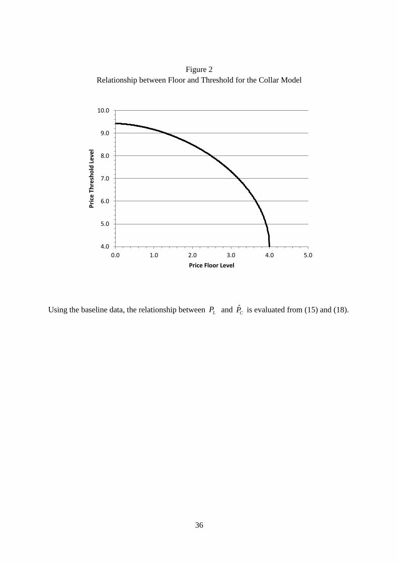
the option coefficient 0CA from (19). As expected, the threshold declines as LP increases

within its allowable range, showing that an earlier exercise is achievable only for improvements

in the floor. The locus relating the threshold ˆCP with the floor

LP defined by (18) is illustrated

in Figure 2, which reveals not only the feasible limits of ˆCP and

LP , but also their negative

relationship. In contrast, the choice of cap HP has no effect on the threshold and the timing

decision. In Panel B of Table 3, the option coefficient is observed to move in line with positive

changes in LP or .HP A

LP increase raises the extent of the downside protection thereby

15

making the investment option more attractive, while a HP increase reduces the extent of the

upside sacrifice thereby making it more valuable. In Table 3, the results for the floor model are

obtainable from the row where HP , and for the cap model from the column where 0LP

.

***Table 3 and Figure 2 about here***

The relationship between the before and after exercise investment value, with and without a

collar, and price is illustrated in Figure 3. We select the collar levels as 4.0LP and 20.0HP

, which yield a threshold of ˆ 4.000CP and option coefficient 0 2.5270CA . Despite having

a higher threshold level, which suggests an earlier exercise for the collar variant if exercised,

the collarless variant is always more favourable for the concessionaire by having a greater

option coefficient.

***Figure 3 about here***

The cost of the subsidy can be neutralized and the collar made “costless” by suitably

engineering its floor and cap levels. For the ACTIVE concessionaire, or for an investor owning

an ACTIVE project, a “costless collar” might be obtained from a third party equating the

written call and protective put 1 2

21 22 for C C L HA P A P P P P . For instance, for base case

parameter values when P=6, PL=4, PH=15.6, 1 2

21 22 .C CA P A P

For the INVEST opportunity, a “costless collar ” might be designed in the following way: (i)

the without-collar option coefficient 0A is evaluated from (8), (ii) for some pre-specified value

of the collar threshold ˆCP , perhaps equalling the prevailing price, the implied floor

LP can be

determined from (18) (19) because of its invariance with HP , and finally (iii), by setting

0 0CA A the implied cap is determined from (19). Some illustrative “costless” LP and

HP pairs

are presented in Table 4. The pairs are inversely related, as expected, since for the collar to

remain “costless”, any increase in the floor and reduction in downside risk has to be

compensated by an additional sacrifice in upside potential.

***Table 4 about here***

In the presence of a stochastic output price, a collar option can be designed that protects the

investor from downside risk by limiting adverse prices to a floor while simultaneously

16

compelling the investor to forego favourable prices above a cap. This trade-off between upside

potential and downside risk can be engineered to make the collar-variant to be more valuable

as well as supporting an earlier exercise. The floor and cap affect the solution in distinct ways.

Variations in HP have no effect at all on the investment threshold, but the sacrifice of additional

upside potential is reflected in decreases in the investment option coefficient. In contrast, an

improvement in LP and reduction in downside risk produces both a fall in investment threshold

prompting an earlier exercise and a rise in the investment option coefficient making it more

valuable. When designing a collar, initial attention focuses on the floor in determining the

threshold for ensuring the investment has a timely exercise, and then on the cap in assessing

the extent of the value created by the floor is to be sacrificed. While a viable floor increase for

a collar motivates early exercise as well as enhancing its attractiveness, a cap decrease incurs

a sacrifice leading to a reduction in its attractiveness.

4.2.1 Changes in Volatility

In the absence of a collar, a volatility increase is known to accompany a rise in both the

investment threshold and investment option value, Dixit and Pindyck (1994). By using base

case values except that the volatility varies incrementally up to a maximum of 50%, we

compare the impact of volatility changes on the with- and without-collar solutions for 3LP

and 500HP . The threshold for the without-collar variant is shown in Figure 4 to increase at

a faster rate as volatility increases as expected because 0LP and 0ˆ ˆCP P , so the with-collar

variant possesses a lower threshold and an earlier timing for all positive .

The comparative timing decisions for the with- and without-collar variants remain essentially

unaltered in the presence of a volatility change, because if 0LP then 0ˆ ˆCP P while if 0LP

then 0ˆ ˆCP P for all positive . However, a volatility increase can produce a distinctive change

in the with-collar option value, which can result in a change of the more preferred variant. If

for low , the chance of a price trajectory penetrating the cap is insignificant, then the

magnitude of the switch option coefficient 21CA is similarly insignificant and consequently the

option coefficient is virtually unaffected. However, as increases, the chance of penetrating

the cap becomes increasingly significant and likewise the coefficient 21CA , with the

consequence that increases in the with-collar option coefficient begin to retard and falter

enabling the without-collar option coefficient to assume dominance. In the design of a collar,

17

if a concessionaire perceives a likely volatility increase to be imminent, then the cap has to be

adjusted upwards to ensure its acceptance by the investor community.

*** Figure 4 about here ***

5 Who Wins, Who Loses, Why?

In the principal-agent problem (GOV-CON) and risk-sharing aspects of collar and floor or

ceiling only arrangements, who wins, and who loses, as parameter values change are likely to

be the indicators for CON versus GOV incentives after the initial transaction. For an ACTIVE

project post-investment with various PPP arrangements, it is assumed that the CON pays the

“fair value” of the concession to the GOV initially. In the base case, we also assume that the

GOV has offered the CON a “costless” real collar arrangement, where the value of a CALL

written by the CON to the GOV on upside revenues higher than the ceiling RH and a PUT

written by the GOV to the CON on downside revenues lower than a floor RL are equal and

RL<R<RH. Both the CON and the GOV agree on the initial parameter values. The effect of

changes in the parameter values can be divided generally into zero-sum games (where the CON

gain/loss is equal to the GOV loss/gain, so that the CON plus GOV profit is zero), constant-

sum games, and variable-sum games (where the CON gain/loss less the GOV loss/gain varies).

Changes in revenue volatility, interest rates, floor level, and ceiling level are zero-sum games,

while changes in revenue and yield are variable-sum games, that is both CON and GOV benefit

or both lose as the parameter values change, but not always by the same magnitude.

ACTIVE

We show here six examples of CON versus GOV results, as parameter values change (see a

complete description of these and other results in the Supplementary Appendix A (ACTIVE)

and B (INVEST). In Figure 5, from an initial “costless” collar if RL=4 and RH =15.6 and R=6,

if R increases, both CON and GOV benefit in a variable-sum game, but on the upside the CON

benefit less than the GOV due to the negative CALL increasing more than the PUT. But, the

CON loses less than the GOV on the downside due to the minimum revenue guarantee.

*** Figure 5 about here ***

18

In Figure 6, from an initial volatility of 25%, if volatility increases, in a zero-sum game (where

the benefits and costs change, but remain equal to each other) the CON suffers from the

negative CALL increasing more than the PUT, and GOV benefits. If volatility decreases from

25%, CON benefits from the negative CALL decreasing less than the PUT, but when the

volatility is close to zero, neither is of any value, thereby reverting to a costless collar.

*** Figure 6 about here ***

Since the GOV profit is increased when volatility increases past 25%, the GOV should

welcome R volatility increases, and the CON strive for decreased volatility, perhaps through

dynamic pricing or issuing debt instruments tied to revenue or traffic levels, or through hedging

if possible.

In Figure 7, from an initial interest rate of 4%, if the interest rate decreases, CON benefits from

the negative CALL decreasing and the PUT increasing significantly. If the interest rate

increases from 4%, CON suffers from the negative CALL increasing and the PUT decreasing

, and GOV experiences the opposite effect. So the CON might seek to protect herself from

interest rate increases by entering into fixed rate loans to fund infrastructure investments, but

with prepayment conditions which allow refinancing if interest rates decrease.

*** Figure 7 about here ** *

In Figure 8, changes in the asset yield result in a highly variable-sum game for the CON and

GOV. From an initial yield of 4%, if the yield decreases, CON benefits from the PV (R/)

increasing less the negative CALL increasing (which benefits the GOV). If the yield increases

from 4%, CON benefits from the negative CALL decreasing and the PUT increasing , offset

by the PV decreasing. GOV suffers from the negative CALL decreasing. The so-called asset

yield, dividend, or convenience yield, or return “shortfall” is a difficult concept to interpret in

most applications, illustrated in this case. The GOV might seek to benefit protect herself by

restricting the payouts of the CON, or by hedging using a term structure of revenue futures, but

since the revenue is probably not a traded security, it is hard to imagine how GOV could realize

this benefit practically.

*** Figure 8 about here ** *

It is interesting to compare collar arrangements with different floors and ceilings, and with

floor only or ceiling only arrangements. Figure 9 shows the risk sharing collar arrangements

19

between CON and GOV as a function of different levels of the floor. It is natural that the CON

benefits (and the GOV suffers) from higher floors, in a zero-sum game.

*** Figures 9 and 10 about here ** *

Equally dramatic in a zero-sum game is the effect of changes in revenue volatility on risk

sharing when there is only a floor, or alternatively only a ceiling. Figure 10 shows the risk

allocation with a floor only as a function of R volatility, but with the CON benefit increasing

with volatility up to a certain point (about 45%), when thereafter volatility increases result in a

decline of the CON benefit.

6 Two Additional Cases

We now consider two illustrative cases, case-A and case-B, to investigate whether the findings

for the plain vanilla collar formulation concerning the nature of the investment threshold and

option coefficient extend to more complicated collar designs. In case-A, we increase the

number of regimes by 1 and formulate the shared revenue for the outer regimes of the collar to

depend on a proportion of the revenue and not on a constant as for the vanilla version. Our

findings for this revision demonstrate that an analytical solution is obtainable despite the

increase in complexity. Some of the sensitivities to changes in parameter values are similar to

the previous collar model, but some are surprising. Similarly, the number of regimes for case-

B, is also increased by 1, but there is also the possibility of giving the investor a “sell-out” or

exit option. This revision does produce a notable change in the resulting solution compared

with the plain vanilla findings, which is due to the altered switch option structure. The notation

we use in section 6.1 and 6.2 are specific to each of those 2 sections, except that 1 and 2 are

specified by (4).

6.1 Case-A Partial Put and Partial Call

Shaoul et al. (2012) report that for a U.K. rail franchise agreement, investors are reimbursed

for 50% of any revenue shortfall below 98% of forecast and 80% below 96%, but suffer a claw-

back of 50% of revenue exceeding 102%, equivalent to partial puts and calls. In case-A, we

amend this arrangement as follows. The actual revenue generated from operating the franchise

through making an irrecoverable investment with cost K is denoted by X . For the purpose of

determining the revenue to be received by the investor, the agreement with the government

divides the revenue schedule into 4 distinct exhaustive regimes. The 3 junctions for

neighbouring regimes occur at LLX X , where

LLX represents the lowest limit, at LX X

20

where LX is the lower limit, and at

UX X where UX is the upper limit, with

LL L UX X X

. Under Regime I with LLX X , the “revenue received” by the concessionaire is the actual

revenue X plus a proportion 1 LLw of the shortfall below forecast, under Regime II with

LL LX X X , revenue received is X plus a proportion 1 Lw of the shortfall below forecast,

where 0 1LL Lw w , under Regime III with L UX X X , revenue received is X , and

under Regime IV with UX X , the revenue received is X less a proportion 1 Uw of the

excess over forecast where 0 1Uw . In the absence of any fixed costs and taxation, the

regime value is determined not only from the revenue schedule but also from the presence of

any switch options.

For each regime, if there exist opportunities for switching to an upper or lower neighbouring

regime, then these are represented by options, a call-style option for upward switching and a

put-style option for downward switching, so both Regime II and III are characterized by both

call and put options, while Regime I by a call and Regime IV by a put. Also, a switch producing

a revenue advantage is represented by a positive option value coefficient, while that for a

revenue disadvantage by a negative coefficient. The specification and associated revenue

values for each of the four regimes are listed in Table 5.

Table 5

Regime Specification and Revenue Schedule for Case-A

Regime Specification Value

I LLX X

1

11

1

I

L L L LL LLLL

V X A X

w X w w Xw X

r r

II LL LX X X

1 2

21 22

1

II

L LL

V X A X A X

w Xw X

r

III L UX X X 1 2

31 32IIIV X A X A X

X

21

IV UX X

2

42

1

IV

U LU

V X A X

w Xw X

r

The six unknown switch option coefficients, 11 21 22 31 32 42, , , , ,A A A A A A , are determined from the

value matching relationships and associated smooth pasting conditions. The value matching

relationships, defined at each of the 3 junctions of neighbouring regimes are, respectively:

0LL

II IX X

V X V X

(22)

0L

III IIX X

V X V X

(23)

0U

IV IIIX X

V X V X

(24)

Equations (22)-(24) together with the 3 associated smooth pasting conditions are sufficient to

solve for the unknowns. The resulting solutions together with their signs are presented in Table

6 in their order of calculation. The coefficients having a positive value indicate that the

corresponding switch options are owned by the investor and contribute to their investment

value, whilst those having a negative sign are sold and detract from the investment value.

Table 6

Case-A Solutions and Conditions for the Switch Option Coefficients Partial Collar Model

Coefficient Solution Condition

2

1 1

22

1 2

1L LL LL

LL

w w X rA

r X

22 0A

1

2 2

31

1 2

1 1U U

U

w X rA

r X

31 0A

1

2 2

21 31

1 2

1 1L L

L

w X rA A

r X

21 0A

2

1 1

32 22

1 2

1 1L L

L

w X rA A

r X

32 0A

2

1 111 21 22

L LL LLLL

LL LL

w w X rXA A A

X r X

11 0A

22

1

2 242 31 32

1 L UU

U U

w X rXA A A

X r X

42 0A

The optimal exercise of the investment opportunity is characterized by the unknown revenue

threshold denoted by 0X̂ , which is derived from the value matching relationship and optimality

condition. At 0ˆX X , the opportunity value, 1

0 0ˆA X

with unknown coefficient 0 0A , is

sufficient to compensate the value of net revenue generated by the project, less the investment

cost K, plus the values of any available switch options. For the purpose of analysis, we presume

that exercise occurs for L UX X X , where the revenue enjoys its greatest incremental rate.

The value matching relationship is:

1 1 200 0 31 0 32 0

ˆˆ ˆ ˆX

A X K A X A X

(25)

Due to the similarity between (16) and (25), it is straightforward to deduce that 0X̂ and 0 0A

are given by, respectively:

20 1 1 232 0

1 1

ˆˆ

1 1

XK A X

(26)

1

2 1

1

0 20 32 0 31

1 2 1

02 2 0 31

1 2

ˆ 1 ˆ1

ˆ1 ˆ1 .

KXA A X A

XK X A

(27)

Equations (26) and (27) reveal that while the investment threshold 0X̂ depends only on 32,A

the option coefficient 0A depends on both

31A and 32A . This result echoes the findings for the

plain vanilla collar formulation. The investment threshold depends on 32A , which depends on

the floor-like attributes LX and

Lw , and on 22A , which also depends on the floor-like attributes

LLX and LLw . The threshold is determined by only floor-like attributes. Similarly, the option

value depends not only on 32A but also

31A , which depends on the cap-like attributes UX and

Uw . The investment option value is determined by both floor- and cap-like attributes. A

systematic approach for a government in deciding suitable values for the floor- and cap-like

attributes is identify the threshold level, which may be aligned to the prevailing level to ensure

immediate exercise, in order to determine the floor-like attributes, and then to invoke policy

23

for identifying a subsidy level, which defined by the difference between the without- and with-

collar option values is used to determine the cap-like attributes. It is interesting to note that

although these findings are based on assuming that 0ˆ

L UX X X , they also result when

assuming that 0ˆ

LL LX X X (for numerical illustrations see the Supplementary Appendix).

6.2 Case-B

We now turn to a more sophisticated version of the collar option also having 4 regime layers

involving a differential tax structure and exit option. Its development combines some aspects

of the models proposed by Rose (1998) and Takashima et al. (2010). A firm in a monopolistic

situation possesses the opportunity to invest in an irretrievable project having a capital

expenditure of K . The revenue generated by the active project denoted by X is described by

a geometric Brownian motion process having identical parameter values as before. Out of

revenue is paid a constant fixed cost f yielding after-tax net revenue of 01X f ,

where 0 is the relevant corporate tax rate. The firm negotiates a contractual agreement with

the government, which offers the firm protection against adverse revenue movements but at

the risk that favourable movements incur higher tax rates. If an adverse movement produces a

net revenue loss 0X f , initially the government then reimburses the firm for the

difference so the net revenue is specified by max ,0X f . For subsequent adverse

movements, the firm has the right to dispose of the project asset to the government for the

amountDK , where

DK K . Optimal disposal occurs as soon as revenue falls to the exit

threshold, ˆDX where ˆ

DX f . In contrast, if the movement is favourable, then the project

attracts a higher tax rate 1 0 for revenues exceeding some pre-specified upper limit

UX .

For subsequent favourable movements where UUX X , with

UU UX X , the revenue is capped

at the pre-specified top upper limit UUX .

There are four identifiable distinct and exhaustive regimes for this collar arrangement, defined

over ˆ ,DX . Regime I is specified by ˆDX X f ; Regime II by the

Uf X X ; Regime

III by U UUX X X ; and Regime IV by

UUX X . For Regimes II and III, embedded options

exist for switching to the neighbouring lower and upper regimes, while for Regime I, there

exists options for switching to Regime II and for disposal, and for Regime IV, an option for

24

switching to Regime III. The regime specifications and values , , , ,JV J I II III IV are

reproduced in Table 7.

Table 7

Regime, Specification and Value for Case-B

Regime Specification Value

I ˆDX X f 1 2

11 12IV X A X A X

II Uf X X

1 2

21 22

0 01 1

IIV X A X A X

X f

r

III U UUX X X

1 2

31 32

1 1 1 01 1

III

U

V X A X A X

X f X f

r r

IV UUX X

2

42

1 1 01

IV

UU U

V X A X

X f X f

r r

At the disposal junction and at each of the three junctions having neighbouring regimes, there

is a value matching relationship:

ˆ

0D

I DX X

V X K

(28)

0II IX f

V X V X

(29)

0U

III IIX X

V X V X

(30)

0UU

IV IIIX X

V X V X

(31)

The 4 equations (28)-(31) together with the 4 associated smooth pasting conditions are

sufficient for solving the 8 unknowns 11 12 21 22 31 32 42ˆ, , , , , , , DA A A A A A A X 2. The solutions, which

are evaluated in the order of presentation, are presented in Table 8 together with any conditions.

2 Note that KD has to be specified so that ˆ0 DX f .

25

Table 8

Case-B Solutions and Conditions for the Switch Option Coefficients

1

2 2 1

31

1 2

1 1UU

UU

X rA

r X

0

1

2 2 1 0

21 31

1 2

1U

U

X rA A

r X

0

1

2 2 0

11 21

1 2

1 1f rA A

r f

0

1

1

2

11 1 2

ˆ DD

KX

A

ˆ0 DX f

2

112

1 2ˆ

D

D

KA

X

0

1

2 2

0 1 11 21

22 12

2 2

1f A A fA A

f f

0

1

2 2

1 0 1 21 31

32 22

2 2

U U

U U

X A A XA A

X X

0

1

2 2

1 1 3142 32

2 2

1UU UU

UU UU

X A XA A

X X

0

The investment threshold 0X̂ is determined as before. At 0ˆX X , the opportunity value 1

0 0ˆA X

where 0 0A equals the generated net value plus any switching options. The net value depends

on the relevant regime at exercise, which we presume occurs during Regime II because of its

higher net revenue and lower tax rate, so the net value is given by IIV X K . The value

matching relationship is given by:

1 1 20 0 0

0 0 21 0 22 0

ˆ 1 1ˆ ˆ ˆX fA X A X A X K

r

(32)

From (32) and its associated smooth pasting condition, the investment threshold is obtained

numerically from:

26

20 0 01 1 222 0

1 1

ˆ 1 1 ˆ1 1

X fK A X

r

(33)

and the option coefficient from:

1

2 1

1

0 0 20 22 0 21

1 2 1

0 0 0

2 2 0 21

1 2

ˆ1 1 ˆ1

ˆ 1 11 ˆ1 .

Kr f XA A X A

r

X Kr fX A

r

(34)

In the absence of any collar arrangement, but retaining the lower tax rate, the investment

threshold 00X̂ and option coefficient 00A are given by standard theory as, respectively:

00 0 1

0

1

ˆ 11

1

XrK f

r

(35)

1 1

0 0 0

00

1 0 1 0

ˆ 1 1.

ˆ ˆ1

X Kr fA

X r X

(36)

From (33) and (34), respectively, the investment threshold 0X̂ depends on 22A while

0A

depends on both 22A and

21A . This result is similar to the plain vanilla collar formulation, but

with an important exception. Whilst for the plain vanilla collar, 21A depend on the floor and

cap attributes and 22A on floor property alone, respectively, for case-B, they both depend on

both attributes. The value of 22A is composed of 3 components: the first depends on the fixed

cost, a basis for the floor specification, the second on the difference between 11A and

21A , and

third on 12A . The difference

11 21A A similarly depends on only the fixed cost, but 12A depends

on 11 21 31ˆ , , ,DX A A A , where

21A and 31A depend on

UX and UUX , bases for the cap specification.

The values of both the investment threshold and option coefficient are influenced by both the

floor and cap attributes.

The explanation underpinning the dependence of the case-B investment threshold on both the

floor and cap attributes hinges on its distinctive collar design. Unlike the plain vanilla variant

which permits switching between all neighbouring regimes, there is no recourse in the case-B

design to revert back to operating the active asset following its disposal. The plain vanilla and

case-B designs are subtly different, a distinction causing the threshold for the latter to depend

on both the floor and cap attributes (see the Supplementary Appendix).

27

The ACTIVE Case A and B collars have somewhat different sensitivities to changes in P and

P volatility. ACTIVE Case B partial collars combined increase more or less linearly with

increases in P, while Case A partial collars with the parameter values in the Supplementary

Appendix, the same proportional sharing over the regimes, show a decreasing sensitivity to

increases in P. The sensitivity of Case A and B to changes in P volatility (“vegas”) are

substantially different, with the VC partial collar A hardly changing as volatility increases, but

the VC partial collar B decreases sharply with volatility increases (see the Supplementary

Appendix).

The INVEST Case A and B collars have substantially different sensitivities to changes in P and

P volatility. INVEST Case B partial collars combined increase with increases in P, while Case

A partial collars first increase and then decrease with increases in P. The sensitivity of Case A

and B to changes in P volatility are opposite, with the VC partial collar A increasing as P

volatility increases, but the VC partial collar B decreases sharply with volatility increases. The

implications are that a prospective concessionaire expecting volatility increases in the future

would not expect to be compensated post-investment in Case A, but would for Case B, but for

pre-investment combined options the concessionaire would appreciate increased volatility in

the underlying P in Case A arrangements, but not for Case B schemes (see the Supplementary

Appendix).

Note that the incentives for volatility management of the concessionaire who is interested in

maximizing ROV pre-investment are completely different for the case A and B arrangements.

The concessionaire should prefer to reduce volatility both pre-investment for Case B (increases

ROV) and post-investment (ACTIVE), but not necessarily for Case A arrangements.

Governments seeking early investment should prefer reduced volatility in both cases.

7 Conclusion

In a mainly analytical way, the properties of a plain vanilla collar, made up of a floor and cap,

are investigated for an active asset using a real option formulation. The collar is composed of

pairs of American perpetuity put and call options that confine a focal variable, such as revenue,

price or volume, to a designated field specified by the floor and cap. We demonstrate that

provided that the floor is positive and selected from its feasible domain, then the investment

28

threshold for a with-collar is always less than that for a without-collar asset opportunity. Under

these conditions, the with-collar investment opportunity is exercised earlier and by inducing

investment, the collar acts in a similar way as an investment subsidy. Whether the with-collar

opportunity should be exercised in preference to the without-collar alternative depends on the

relative magnitudes of their investment option values. Although only the floor governs the

investment timing, both the floor and the cap are crucial in determining the real option value

of the investment opportunity, but in opposing ways. The floor provides partial if not complete

protection against the downside risk of the net cash flows rendered by the with-collar asset

being insufficiently viable, and any feasible increase in the floor is associated with

improvements in the investment value. In contrast, the cap affects only the investment value

by controlling the magnitude of the upside potential that the investor foregoes, and any cap

reduction enhances this sacrifice with a consequential loss in option value.

Only the floor of the collar governs the investment threshold while both the floor and cap

impact on the option value, but in opposing directions. Normally, the threshold exceeds the

zero NPV level in order to moderate the extent that future net cash flows are non-viable, and

greater volatility values are reflected in higher thresholds. Since a floor mitigates this extent,

its presence necessarily lowers the threshold while simultaneously enhancing the opportunity

value. In contrast, the cap representing a sacrifice to the investor depresses the opportunity

value and reduced cap levels are reflected in lower opportunity values. Further, since a

specified cap level gains in significance as the volatility increases, a with-collar variant may be

preferred at lower volatilities while the without-collar variant may be preferred by the

concessionaire at higher volatilities.

As a form of subsidy, the collar can be designed to clawback high profits as well as inducing

early investment or even immediate investment. The role of the cap is to mitigate the cost to

the government of guaranteeing a floor, and thereby inhibits the spread of any allegations of

being over-generous. Governments can even create a “costless” collar by selecting a floor to

induce investment and a cap that neutralizes the additional value it creates. A collar shares the

benefits of a more conventional subsidy-taxation model for inducing investment with the

additional merit of not having to incur an immediate subsidy payment.

We provide an analytical framework for viewing the real option value of various PPP

arrangements, ranging from no collar, floor only, ceiling only, and a collar (both floor and

29

ceiling). One use of this framework is to identify clearly the gains and losses for a principal

(GOV) and agent (CON) participants in a PPP infrastructure project as parameter values

change. Different real option games are envisioned, where changes in the parameter values

after an initial deal result in zero-sum games, or constant-sum games, or variable-sum games.

This basic framework may be useful in viewing the intended consequences of different

appropriate PPP arrangements, and in identifying incentives for the agent in holding an

investment opportunity or in operating an infrastructure facility.

The plain vanilla collar is extended in two directions. The first considers a design where the

floor and cap attributes are not constant but depend on the focal variable. This demonstrates

that the previous findings continue to hold, that the threshold is determined by only the floor

attributes while the option value is determined by both the floor and cap attributes. This

facilitates the engineering of the collar design, since adjustments to the floor attributes are first

made to yield the desired threshold and then the cap attributes are adjusted to meet the desired

government contribution. The second extension involves an exit option, which does not allow

any return to operating the active asset following its disposal. For this design, the plain vanilla

findings do not hold as both the floor and cap attributes influence the threshold and option

value.

There are several implicit assumptions behind our analytical framework. (i) The arrangements

are perpetual American call or put options, and a perpetual series of cash flows, viewed in

continuous time. Real arrangements may not perpetual, so both the options and the cash flows

would have to be reformatted as perpetuals less forward start options, or finite annuities,

especially for short-term arrangements and low discount rates. This may not be a significant

problem for 100 year arrangements when discount rates are high. (ii) Parameter values such

as interest rates, yield, revenue volatility, revenue floors and ceilings are considered constant

or deterministic. Relaxing some of these assumptions is an interesting extension. (iii)

Sometimes PPP arrangements specify that the concession termination is based on a specified

achieved internal rate of return, or cumulative net present value, or accumulated net cash flows.

We do not focus on negotiated exit prices or for CON or GOV determined exit timing, except

for Case B. (iv) PPPs are assumed to be monopolies, without competition or unexpected

failures or physical disasters. (v) The framework models are viewed in continuous time

whereas revenue (especially traffic), minimum and maximum revenue compensations and

payments are likely to occur in discrete time. (vi) We do not allow for operating costs that are

30

not already included in net revenues, or for periodic maintenance requirements. (vii) The

revenue stream ignores other possible real options such as project cancellation, downsizing,

renegotiation, expansion and resale, dynamic pricing for times of usage, and extensions into

other activities such as retail activities for motorway operators. (viii) PPP arrangements are

envisioned as enforceable, without credit or default risk for either party, and investments are

irrevocable, immediate, and terms cannot be re-negotiated over time. (ix) While many of the

PPP infrastructure arrangements cited herein concern transportation, other PPP arrangements

such as building and operating hospitals and educational establishments may not have clear

objectives such as sharing revenue risks and benefits. Suitably designed optional elements may

incorporate some of same, or conceivably completely different objectives. Most of these issues

present interesting aspects for future research.

31

8. References

Alonso-Conde, A. B., C. Brown, and J. Rojo-Suarez. "Public private partnerships: Incentives,

risk transfer and real options." Review of Financial Economics 16 (2007), 335-349.

Alvarez, L. “Optimal exit and valuation under demand uncertainty: A real options approach”

European Journal of Operational Research, 114 (1999), 320-329.

Armada, M. R. J., P. J. Pereira, and A. Rodrigues. "Optimal subsidies and guarantees in public–

private partnerships." The European Journal of Finance 18 (2012), 469-495.

Atlantica. "Annual Report". (2015).

Azevedo, A. and D. Paxson. “Developing real option game models” European Journal of

Operational Research 237 (2014), 909-920.

Blank, F. F., T. K. N. Baidya, and M. A. G. Dias. "Real options in public private partnerships:

A case of a toll road concession." In Real Options Conference. Braga, Portugal (2009).

Bowe, M., and D. L. Lee. "Project evaluation in the presence of multiple embedded real

options: evidence from the Taiwan High-Speed Rail Project." Journal of Asian

Economics 15 (2004), 71-98.

Brandão, L. and E. Saraiva. “The option value of government guarantees and infrastructure

projects”, Construction Management and Economics 26 (2008), 1171-1180.

Brown, C. "Financing transport infrastructure: For whom the road tolls." The Australian

Economic Review, 38 (2005), 431-438.

Carbonara, N., N. Costantino and R. Pellegrino. “Revenue guarantee in public-private

partnerships: a fair risk allocation model”, Construction Management and Economics 32

(2014), 403-415.

Chevalier-Roignant, B., C. Flath, A. Huchzermeier and L.Trigeorgis. “Strategic investment

under uncertainty” European Journal of Operational Research 215 (2011), 639-650.

Clark, E. and J.Z. Easaw. “Optimal access pricing for natural monopoly networks when costs

are sunk and revenues are uncertain” European Journal of Operational Research 178 (2007),

595-602.

Dixit, A. K., and R. S. Pindyck. Investment under Uncertainty. Princeton, NJ: Princeton

University Press (1994).

Huang, Y. L., and S. P. Chou. "Valuation of the minimum revenue guarantee and the option to

abandon in BOT infrastructure projects." Construction Management and Economics 24

(2006), 379-389.

32

Merton, R. C. "Theory of rational option pricing." Bell Journal of Economics and Management

Science 4 (1973), 141-183.

—. Continuous-Time Finance. Oxford: Blackwell Publishing (1990).

National Audit Office. "Nuclear power in the U.K.", London: HM Stationary Office (2016)

Páez-Pérez, D. and M. Sándhez-Silva. “A dynamic principal-agent framework for modeling

the performance of infrastructure” European Journal of Operational Research 254 (2016),

576-594.

Rose, S. "Valuation of interacting real options in a tollroad infrastructure project." The

Quarterly Review of Economics and Finance 38 (1998), 711-723.

Samuelson, P. A. "Rational theory of warrant pricing." Industrial Management Review 6

(1965), 13-32.

Scandizzo, P.L. and M. Ventura. “Sharing risk through concession contracts” European

Journal of Operational Research 207 (2010), 363-370.

Shan, L., M.J. Garvin and R. Kumar. “Collar options to manage revenue risks in real toll public-

private partnership transportation projects”, Construction Management and Economics 28

(2010), 1057-69.

Shaoul, J., A. Stafford, and P. Stapleton. "The fantasy world of private finance for transport via

public private partnerships." OECD Publishing, Discussion Paper No. 2012-6 (2012).

Takashima, R., K. Yagi, and H. Takamori. "Government guarantees and risk sharing in public–

private partnerships." Review of Financial Economics 19 (2010), 78-83.

33

Appendix

Price Floor Model

We use the additional subscript f to indicate a model with only a floor. From (10) the active

project valuation function becomes:

1

2

11

22

for

for ,

LCf L

Cf

Cf L

P YA P P P

rV P

PYA P P P

(A1)

with:

1 2

2 2 1 1

11 22

1 2 1 2

0, 0.L L

Cf Cf

L L

P Y r r P Y r rA A

P r P r

(A2)

The investment option value is specified by:

1

2

0

0

22

ˆ for

ˆ- for ,

Cf Cf

C f

Cf Cf

A P P P

F P PYA P K P P

(A3)

with ˆ ˆCf CP P determined from (18) with 22CA replaced by

22CfA , and the investment option

coefficient by:

1

0 2 2 0

1 2

ˆ1 ˆ1 CCf C

P YA K P A

. (A4)

A feasible floor for an active asset yields both a more valuable investment opportunity and one

that is exercisable at an earlier time. Consequently, a floor represents a government granted

subsidy, Armada et al. (2012).

Price Cap Model

We use the additional subscript c to indicate a model with only a cap. From (10) the active

project valuation function becomes:

34

1

2

21

32

for

for ,

Cc H

Cc

HC H

PYA P P P

V PP Y

A P P Pr

(A5)

with:

1 2

2 2 1 121 32

1 2 1 2

0, 0H HCc Cc

H H

P Y r r P Y r rA A

P r P r

. (A6)

The investment option value is specified by:

1

1

0

0

21

ˆ for

ˆ- for ,

Cc Cc

C c

Cc Cc H

A P P P

F P PYA P K P P P

(A7)

with 0

ˆ ˆCcP P determined from (6), and investment option coefficient:

1

0 21 0

1

ˆ

1

CCc Cc

KPA A A

. (A8)

The imposition of a cap has no effect on the investment threshold and the timing, but it does

produce a less valuable investment option. It is significantly less desirable for the

concessionaire than an opportunity without a cap, and consequently it is imposed by, for

example, a government intent on offering a subsidy while reducing its cost, or by limits to

growth due to firm or market characteristics.

35

Figure 1

Effect of Price on Switch Option Value

at Two Different Floor Levels

Using the baseline data, the switch option value is evaluated from (21) for the indicated LP and

HP values.

36

Figure 2

Relationship between Floor and Threshold for the Collar Model

Using the baseline data, the relationship between LP and ˆCP is evaluated from (15) and (18).

4.0

5.0

6.0

7.0

8.0

9.0

10.0

0.0 1.0 2.0 3.0 4.0 5.0

Pri

ce T

hre

sho

ld L

eve

l

Price Floor Level

37

Figure 3

The Effect of Price on the Investment Value

for the With- and Without-Collar Variants

0

50

100

150

200

250

300

350

400

0 5 10 15 20

Val

ue

Price

Without Collar With Collar

The selected floor and cap prices for the collar variant are 4.0LP and 20.0HP

, respectively. The evaluations for the two variants are based on base case values.

The solution values for the collarless variant are 0 2.7547A and 0ˆ 9.4273P ,

while those for the collar variant are drawn from Tables 2 and 3.

38

Figure 4

Effect of Volatility Variations on the Price Thresholds for the

With- and Without-Collar Variants

The evaluations for the two variants are based base case values, and the floor and

cap prices for the collar variant are 3.0LP and 500.0HP , respectively.

4

6

8

10

12

14

16

18

20

0% 10% 20% 30% 40% 50%

Pri

ce T

hre

sho

ld

Volatility

With Collar Without Collar

39

Figure 5

Figure 6

Assumes

At R=2, the CON would have lost -150+50=-100 without the Min R guarantee and ROV, but instead loses -42.

At R=18, the CON would have gained 450-150=300 without the ceiling ceded to the GOV, but instead gains 111.

Assumes the GOV has ceded control over a valuable monopoly, so GOV profit deducts the PV when R=6.

ACTIVE infrastructure is sold to Concessionaire (CON) at fair value R/ when R=6 and

Government (GOV) guarantees a minimum R of 4 and receives all R over 15.60.

At R=6 and the other parameter values, -CALL=PUT for a "costless collar",

so the combined "profit" over the fair value of the CON and GOV is 0.

-200

-100

0

100

200

300

400

2 4 6 8 10 12 14 16 18

R

Revenue Sharing PPP as Function of R

GOV Profit

CON + GOV

CON Profit

CON Profit 0.00 0.98 3.95 4.62 2.99 0.00 -3.64 -7.49 -11.27 -14.84 -18.13 -21.13 -23.82 -26.23 -28.38 -30.29

GOV Profit -Sale 0.00 -0.98 -3.95 -4.62 -2.99 0.00 3.64 7.49 11.27 14.84 18.13 21.13 23.82 26.23 28.38 30.29

Interpretation

At =.01, the CALL and PUT for both the CON and GOV would have been of little value, when R=6.

At =.75, the CALL would be worth 106.14 for the GOV (and -106.4 for the CON), while the PUT would be worth -75.85 for the GOV.

So with these values, the CON would welcome R volatility below 25%, and the GOV benefit from higher volatility.

Assumes the monopoly over which the GOV cedes control is of no value to the GOV.

ACTIVE infrastructure is sold to Concessionaire (CON) at fair value R/ when

Government (GOV) guarantees a minimum R of 4 and receives all R over 15.60.

At R=6 and the other parameter values, -CALL=PUT for a "costless collar",

so the combined "profit" over the fair value of the CON and GOV is 0.

-40

-30

-20

-10

0

10

20

30

40

0.01 0.05 0.10 0.15 0.20 0.25 0.30 0.35 0.40 0.45 0.50 0.55 0.60 0.65 0.70 0.75

R Volatility

Revenue Sharing PPP as function of R Volatility

CON Profit

GOV Profit -Sale

40

Figure 7

Figure 8

Assumes

Assumes the GOV has ceded control over a valuable monopoly, so GOV profit deducts the PV when R=6.

ACTIVE infrastructure is sold to Concessionaire (CON) at fair value R/ when R=6 and

Government (GOV) guarantees a minimum R of 4 and receives all R over 15.60, interest rate is 4%.

At R=6 and the other parameter values, -CALL=PUT for a "costless collar",

so the combined "profit" over the fair value of the CON and GOV is 0.

-300

-200

-100

0

100

200

300

0.01 0.02 0.03 0.04 0.05 0.06 0.07 0.08 0.09

Interest Rate

Risk Sharing as Function of the Interest Rate

GOV Profit

CON + GOV

CON Profit

Assumes

Assumes the GOV has ceded control over a valuable monopoly, so GOV profit deducts the PV when R=6.

ACTIVE infrastructure is sold to Concessionaire (CON) at fair value R/ when R=6 and is 4%.

Government (GOV) guarantees a minimum R of 4 and receives all R over 15.60, interest rate is 4%.

At R=6 and the other parameter values, -CALL=PUT for a "costless collar",

so the combined "profit" over the fair value of the CON and GOV is 0.

-100

0

100

200

300

400

500

0.01 0.02 0.03 0.04 0.05 0.06 0.07 0.08 0.09

Yield

Risk Sharing as a Function of Project Yield

GOV Profit

CON + GOV

CON Profit

41

Figure 9

Figure 10

Assumes

Assumes the GOV has ceded control over a valuable monopoly, so GOV profit deducts the PV when R=6.

ACTIVE infrastructure is sold to Concessionaire (CON) at fair value R/ when R=6 and is 4%. Base case is

GOV guarantees a minimum R of 4 and receives all R over 15.60, interest rate is 4%.

At R=6 and the other parameter values, -CALL=PUT for a "costless collar",

so the combined "profit" over the fair value of the CON and GOV is 0.

-100

-80

-60

-40

-20

0

20

40

60

80

100

1 2 3 4 5 6 7 8 9

RL

Risk Sharing as function of Floor

GOV Profit

CON + GOV

CON Profit

Interpretation

At =.01, the CALL and PUT for both the CON and GOV would have been of little value, when R=6 when there is a floor only.

At =.75, the CALL would be worth 46.93 for the GOV (and -46.93 for the CON), while the PUT would be worth -75.85 for the GOV.

So with these values, the CON would welcome R volatility especially around 45%.

Assumes the monopoly over which the GOV cedes control is of no value to the GOV.

ACTIVE infrastructure is sold to Concessionaire (CON) at fair value R/ when

-50

-40

-30

-20

-10

0

10

20

30

40

50

0.01 0.05 0.10 0.15 0.20 0.25 0.30 0.35 0.40 0.45 0.50 0.55 0.60 0.65 0.70 0.75

R Volatility

RISK ALLOCATION with Floor Only as function of R Volatility

CON Profit

GOV Profit -Sale

Table 2

Switch Option Coefficients for the With-Collar Model for Variations in Floor and Cap Levels

Panel A: 11CA Panel B: 21CA

HP 0LP 1LP 2LP 3LP 4LP HP 0LP 1LP 2LP 3LP 4LP

10 0.0000 8.2537 4.2116 2.6454 1.7862 10 -1.8520 -1.8520 -1.8520 -1.8520 -1.8520 20 0.0000 8.9944 4.9523 3.3862 2.5270 20 -1.1112 -1.1112 -1.1112 -1.1112 -1.1112

50 0.0000 9.5400 5.4979 3.9317 3.0726 50 -0.5656 -0.5656 -0.5656 -0.5656 -0.5656 100 0.0000 9.7663 5.7241 4.1580 3.2988 100 -0.3394 -0.3394 -0.3394 -0.3394 -0.3394 200 0.0000 9.9020 5.8599 4.2937 3.4346 200 -0.2036 -0.2036 -0.2036 -0.2036 -0.2036 500 0.0000 10.0020 5.9599 4.3937 3.5345 500 -0.1037 -0.1037 -0.1037 -0.1037 -0.1037 1000 0.0000 10.0435 6.0013 4.4352 3.5760 1000 -0.0622 -0.0622 -0.0622 -0.0622 -0.0622 Infinity 0.0000 10.1057 6.0635 4.4974 3.6382 Infinity 0.0000 0.0000 0.0000 0.0000 0.0000

Panel C: 22CA Panel D: 32CA

HP 0LP 1LP 2LP 3LP 4LP HP 0LP 1LP 2LP 3LP 4LP

10 0.000 10.106 33.685 68.123 112.280 10 -551 -541 -518 -483 -439 20 0.000 10.106 33.685 68.123 112.280 20 -1838 -1828 -1804 -1770 -1726 50 0.000 10.106 33.685 68.123 112.280 50 -9027 -9017 -8994 -8959 -8915 100 0.000 10.106 33.685 68.123 112.280 100 -30090 -30080 -30057 -30022 -29978 200 0.000 10.106 33.685 68.123 112.280 200 -100299 -100289 -100265 -100231 -100187 500 0.000 10.106 33.685 68.123 112.280 500 -492596 -492586 -492562 -492528 -492484

1000 0.000 10.106 33.685 68.123 112.280 1000 -1641948 -1641938 -1641914 -1641880 -1641836 Infinity 0.000 10.106 33.685 68.123 112.280 Infinity -Infinity -Infinity -Infinity -Infinity -Infinity

Using the baseline data, the coefficients 11 21 22 32, , ,C C C CA A A A are evaluated from (15) for the various indicated LP and HP values.

43

Table 3

Option Threshold and Coefficient Values for the With-Collar Model for Variations in Floor and Cap Levels

Panel A: ˆCP

Panel B: 0CA

HP 0LP 1LP 2LP 3LP 4LP HP 0LP 1LP 2LP 3LP 4LP

10 9.4279 9.1627 8.4930 7.3178 4.0000 10 0.9028 0.9434 1.0513 1.2581 1.7862

20 9.4279 9.1627 8.4930 7.3178 4.0000 20 1.6435 1.6842 1.7920 1.9989 2.5270 50 9.4279 9.1627 8.4930 7.3178 4.0000 50 2.1891 2.2298 2.3376 2.5444 3.0726 100 9.4279 9.1627 8.4930 7.3178 4.0000 100 2.4153 2.4560 2.5638 2.7707 3.2988 200 9.4279 9.1627 8.4930 7.3178 4.0000 200 2.5511 2.5918 2.6996 2.9064 3.4346 500 9.4279 9.1627 8.4930 7.3178 4.0000 500 2.6511 2.6917 2.7996 3.0064 3.5345 1000 9.4279 9.1627 8.4930 7.3178 4.0000 1000 2.6925 2.7332 2.8410 3.0479 3.5760 Infinity 9.4279 9.1627 8.4930 7.3178 4.0000 Infinity 2.7547 2.7954 2.9032 3.1101 3.6382

Using the baseline data, the investment threshold and option coefficient are evaluated from (18) and (19),

respectively, for the indicated LP and HP values. The solutions for the floor and cap models are obtainable from

(18), and from (6), respectively.

Table 4

Illustrative Pairs of LP and

HP for a Investment Opportunity “Costless” Collar

LP 0.5 1.0 1.5 2.0 2.5 3.0 3.5 4.0

HP 9430.5 1780.0 649.94 307.02 164.71 93.963 54.011 27.302 ˆCP 9.350 9.163 8.879 8.493 7.986 7.318 6.375 4.000

0CA 2.755 2.755 2.755 2.755 2.755 2.755 2.755 2.755

21CA -0.012 -0.041 -0.085 -0.148 -0.235 -0.355 -0.534 -0.883

22CA 3.032 10.106 20.437 33.685 49.632 68.123 89.038 112.280