© CHAPPUIS HALDER & CIE Risk management in exotic derivatives trading : Lessons from the recent past The example of interest rate & commodities structured derivatives desks 09/01/2015 By Jérôme FRUGIER (BNP Paribas) & Augustin Beyot (CH&Cie) Supported by Benoit GENEST (CH & Cie) DISCLAIMER The views and opinions expressed in this article are those of the authors and do not necessarily reflect the views or positions of their employers. Examples of products and portfolios described in this article are illustrative only and do not reflect the situation of any precise financial institution.

Welcome message from author
This document is posted to help you gain knowledge. Please leave a comment to let me know what you think about it! Share it to your friends and learn new things together.
Transcript
© CHAPPUIS HALDER & CIE
Risk management in exotic
derivatives trading :
Lessons from the recent past The example of interest rate & commodities structured derivatives desks
09/01/2015
By Jérôme FRUGIER (BNP Paribas)
& Augustin Beyot (CH&Cie) Supported by Benoit GENEST (CH & Cie)
DISCLAIMER
The views and opinions expressed in this article are those of the authors and do not
necessarily reflect the views or positions of their employers. Examples of products and
portfolios described in this article are illustrative only and do not reflect the situation of
any precise financial institution.
© Global Research & Analytics Dept.| 2015 | All rights reserved
16
Table of contents
Risk management in exotic derivatives trading ................................................................................. 17
Abstract ............................................................................................................................................ 17
1. Introduction .............................................................................................................................. 18
2. An accumulation of risky products ............................................................................................ 18
3. When risk comes true - A sudden and unexpected inversion of the EUR curve .......................... 24
4. The consequences - A basic illustration ..................................................................................... 30
5. A problematic shared with other asset classes - Focus on commodities ...................................... 31
6. It could have been avoided... ..................................................................................................... 34
7. Efficient risk management techniques ....................................................................................... 36
A. Bending strategies ............................................................................................................ 36
B. Examples of bending strategies ........................................................................................ 37
C. Manage risk concentration and limits ............................................................................... 38
1. Monitoring observation dates and distance to barrier ................................................... 38
2. Monitoring gamma by barrier strike ............................................................................. 39
D. Stress testing .................................................................................................................... 40
8. Conclusion ................................................................................................................................ 41
Bibliography .................................................................................................................................... 42
© Global Research & Analytics Dept.| 2015 | All rights reserved
17
Risk management in exotic derivatives trading The example of interest rate & commodities structured desks
Abstract Banks’ product offering has become more and more sophisticated with the emergence of financial products tailored to the specific needs of a more complex pool of investors. This particularity has made them very popular among investors. By contrast to liquid, easily understandable “vanilla products” with a simple payoff, “exotic” or structured products have a complex risk profile and expected payoff. As a result, risk management for these structured products has proven to be costly, complex and not always perfect, namely due to their inherent dynamic characteristics inherited from their optionality features. In particular, banks’ traders and investors in financial products with a digital optionality have experienced severe losses, either from pure downward pressure on asset prices or from difficulties to manage the inherent market risks properly. This white paper presents a particular occurrence of this issue on the interest rate market, extends it to commodities, and details some risk management techniques that could have been used in order to avoid losses.
Key words: Barrier, Gamma, Options, Hedging, Exotic, Trading, Derivatives
JEL Classification: G20; G28; G51

© Global Research & Analytics Dept.| 2015 | All rights reserved
18
1. Introduction
One of the riskiest and most technical activities in corporate and investment
banking is trading structured (or exotics) derivatives. The desks in charge of this activity
are supposed to buy or sell, sometimes in size, complex products with exotic, unhedgeable
risks: no liquid two-way market is necessarily available to hedge those risks by exchanging
more simple products. Discontinuous payoffs are a typical case as they can lead to
unexpected, strong variations of the risk exposures of the banks, especially for second-
order exposures like gamma risk.
As part of their activity, structured derivatives trading desks tend to pile up
important exposures to some exotic risks which, in case of a strong and sudden market
move, may become difficult to manage and can lead to important losses. This is precisely
what happened in June 2008, when interest rates structured derivatives desks were struck
by a sudden inversion of the EUR swap curve, which led to an inversion of their gamma
exposure. Many banking institutions lost important amounts on those interest rate
structured activities in a few days only.
This paper is focused on the example of derivatives desks and their behavior when
facing some market moves or inversions, as an illustration of the broader issue of the
management of exotic risks accumulation.
2. An accumulation of risky products
As a good illustration, the problem faced by interest rates structured derivatives desks in June 2008 is strongly related to Spread Range Accrual type products. Typically for this product, the payoff is discontinuous. These products are structured swaps, they are typically indexed on a reference spread between 2 rates of the same curve, e.g. CMS 30Y and CMS 2Y. At the end of each period (month, quarter, year...) the bank pays the following payoff to the counterparty:
� × ��
where F is a fixed rate, n is the number of days of the period when the fixing of the reference spread was above a defined strike K, and N is the total number of days in the period. The payoff of the structured leg of the swap (from the bank's point of view) is shown on figure 1:

© Global Research & Analytics Dept.| 2015 | All rights reserved
19
Figure 1: Payoff of a Spread Range Accrual
This type of products was very popular between 2005 and 2008. A major part of such products were sold with a strike at 0, on spreads like 30Y – 2Y, 30Y – 10Y and 10Y –
2Y. In practical terms, most clients bought this kind of product through a so-called “EMTN” (Euro Medium-Term Note)1. As long as the fixing of the spread was above the strike, they would receive a fixed rate higher than the swap rate with the same term. Some clients with a fixed-rate debt could also have a real interest for such product: by entering this swap, they paid a variable market rate (Libor, Euribor...) plus a funding spread and, if the fixing of the reference spread was above the strike, they received a fixed rate F which was greater than the initial debt rate. Thus these clients could keep the difference and reduce the cost of their debt. Of course, if the reference spread was below the strike, the clients would not receive anything from the bank and would lose a significant amount of money. However, thanks to historical analyses, banks were able to sell massively these Spread Range Accruals: since the creation of the EUR currency, the EUR curve had never been inverted, and the profit for the client was considered “almost sure”.
From the trader's point of view, as long as the spread was above the strike, which means as long as the curve was not inverted, the risk management of the product remained simple. To value this discontinuous payoff, a market consensus was to use a piecewise linearization, by valuing a combination of caps on spread, as we can see on figure 2:
1 “A medium-term note (MTN) is a debt note that usually matures in 5–10 years, but the term may be less
than one year or as long as 100 years. They can be issued on a fixed or floating coupon basis. Floating rate
medium-term notes can be as simple as paying the holder a coupon linked to Euribor +/- basis points or can
be more complex structured notes linked, for example, to swap rates, treasuries, indices, etc. When they are
issued to investors outside the US, they are called "Euro Medium Term Notes".” (Source: Wikipedia)

© Global Research & Analytics Dept.| 2015 | All rights reserved
20
Figure 2: Piecewise-linearized payoff
This figure shows clearly that the Spread Range Accrual linearized payoff is
equivalent to selling a cap on the spread at strike � � � and buying a cap on the spread at
strike �, the 2 caps being leveraged at � �⁄ . The � factor was chosen by the trader, usually around 10 to 20 bps. This linearization allows valuing this payoff as a simple linear combination of vanilla products, and ensures conservativeness as the amount to be paid to the client is overestimated.
The models used by banks to value this payoff are complex, using stochastic volatilities of the spread, in order to better simulate smile profiles for each component of the spread. Moreover, the product is in fact a sum of daily digital options, which complicates the valuation further. In this study, for clarity’s sake, we will simplify the payoff as a single digital option on spread S with maturity T and strike K. By using a simple Gaussian model, we can value this single digital option and calculate its sensitivities.
In the following calculations we consider a digital option at strike K, with maturity T, and height H. As we have seen above, it can be piecewise linearized and valued as the
sale of a cap on spread S at strike � � � and the purchase of a cap on spread S at strike K. We assume that the spread, the value of which is S at time t = 0, evolves according to the following equation:
� � ∙ � � � ∙ �� The parameters of this model are the spread evolution tendency , its volatility �,
and the risk-free rate r. It is a normal model, which means that the spread S follows a
Gaussian distribution. Then the value �� of the cap at strike K and maturity T can be obtained easily with Black’s formula2:
2 Iwasawa, K. (2001), Analytic Formula for the European Normal Black Scholes Formula

© Global Research & Analytics Dept.| 2015 | All rights reserved
21
���, �, �, , �, �� � ���� �� � � � �� �1 �! "� � � ��√� $% � �& �2( ��)*"+�,�-�.√� $/0
where ! is the standard normal cumulative distribution function:
!�1� � 1√2(2 ��3/* 45�6
The digital option is a sale of a cap at strike � � � and leverage 7 �⁄ , and a purchase of a cap at strike K and leverage 7 �⁄ . The value �8 of the digital option is easily calculated:
�8�, �, �, , �, �� � �7� :;<�, � � �, �, , �, �� � 7� :;<�, �, �, , �, �� � 7� ���� =�� � � � � � �� �1 �! "� � � � � ��√� $%
��& �2( ��)*"+�>�?�-�.√� $/
�� � � � �� �1 �! "� � � ��√� $%��& �2( ��)*"+�?�-�.√� $/0
Now we will calculate the basic sensitivities (also called greeks) of this payoff:
• delta @: defined as the variation of the value of the digital option when the level of spread S moves
• gamma A: defined as the variation of the delta of the digital option when the level of spread S moves (second order sensitivity)
• vega B: defined as the variation of the value of the digital option when the volatility � moves.
Mathematically, starting with the formula �8 for the digital option value, we obtain the following formulas for greeks:
@ � C�8C � 7� ���� �! "� � � � � ��√� $ �! "� � � ��√� $%

© Global Research & Analytics Dept.| 2015 | All rights reserved
22
A � C*�8C* � 7� �����√2(� D��)*"+�?�-�.√� $/ � ��)*"+�>�?�-�.√� $/E
B � C�8C� � 7� ����& �2( F��)*"+�?�-�.√� $/ � ��)*"+�>�?�-�.√� $/G
The profile of delta, gamma and vega can be seen respectively on figures 3, 4 et5:
Figure 3: Delta profile for the digital option
Figure 4: Gamma profile for the digital option

© Global Research & Analytics Dept.| 2015 | All rights reserved
23
Figure 5: Vega profile for the digital option
We notice that the spread delta is negative: when reference spread increases, the value decreases as the payoff is more likely to be paid. Besides, we notice that the gamma
profile reverses between strikes � � � and K. The vega profile is quite similar to gamma profile.
As long as the spread remains in the area above strike K, the risk management of this product is simple: delta is negative, yet it is not volatile and can be easily hedged with swaps. The vega profile is positive and not volatile, it can be hedged with swaptions. In his daily risk management, the trader faces an exposure that is almost delta-neutral, vega-neutral and gamma-neutral. Observations made for a simple digital option can easily be extended to Spread Range Accrual products.

© Global Research & Analytics Dept.| 2015 | All rights reserved
24
3. When risk comes true - A sudden and unexpected inversion of the
EUR curve
This situation was rather comfortable for structured derivatives trader on rates market, until the first half of 2008. As shown on figure 6, the 30Y – 2Y spread had remained positive:
Figure 6: Evolution of the 30Y – 2Y spread until 30 April 2008
However, in May 2008 the EUR curve began to flatten: 30Y – 10Y and 10Y – 2Y
spreads got closer to 0. Those spreads even became slightly negative, at -3 or -4bps (see figure 7), which was not enough for traders to see their risk exposures move strongly. As a
matter of fact, the use of a � factor to linearize the payoff slightly shifts the inversion of the gamma exposure: instead of happening at strike K, it happens when the spread is between � � � and K. In practical terms, there is a small area just below strike K where the
trader's gamma exposure remains positive, due to the choice of such a cap spread
model, while the gamma of the “real” payoff is already quite negative, as shown on
figure 8. The effect of a slight curve inversion (less than � 2⁄ ) will not be seen by the trader. On the contrary, he will see his gamma exposure become more positive on those products.

© Global Research & Analytics Dept.| 2015 | All rights reserved
25
Figure 7: Evolution of the 30Y – 2Y spread after 1st May 2008
Figure 8: Gamma profiles for discontinuous and linearized payoffs
For that reason, many structured desks could not see the danger of this situation before it was too late. On June 5th 2008, 10 months after the beginning of the subprime

© Global Research & Analytics Dept.| 2015 | All rights reserved
26
crisis, while the Federal Reserve had already cut its main rate from 5.25% to 2% in 6 months, the European Central Bank published its new monetary policy decision: European rates would remain unchanged. In the following press conference, the ECB president Jean-Claude Trichet declared that inflation risks in Europe were still greater than recession risks:
“...we noted that risks to price stability over the medium term have increased
further (...) upside risks to price stability over the medium term are also confirmed
by the continuing very vigorous money and credit growth and the absence of
significant constraints on bank loan supply up to now. At the same time, the
economic fundamentals of the euro area are sound. Against this background, we
emphasize that maintaining price stability in the medium term is our primary
objective in accordance with our mandate...”3
In the following question and answer sequence with journalists, The ECB President was even more explicit about the intentions of the ECB:
“...we consider that the possibility is not excluded that, after having carefully
examined the situation, we could decide to move our rates by a small amount in our
next meeting in order to secure the solid anchoring of inflation expectations, taking
into account the situation. I don't say it is certain, I say it is possible...”4
Rates markets were taken aback. Most analysts had foreseen that the ECB would follow the example of the Fed and emphasize the recession risks in its message, to prepare markets for a rate cut in July 2008, or even sooner. But the actual message was exactly the opposite.
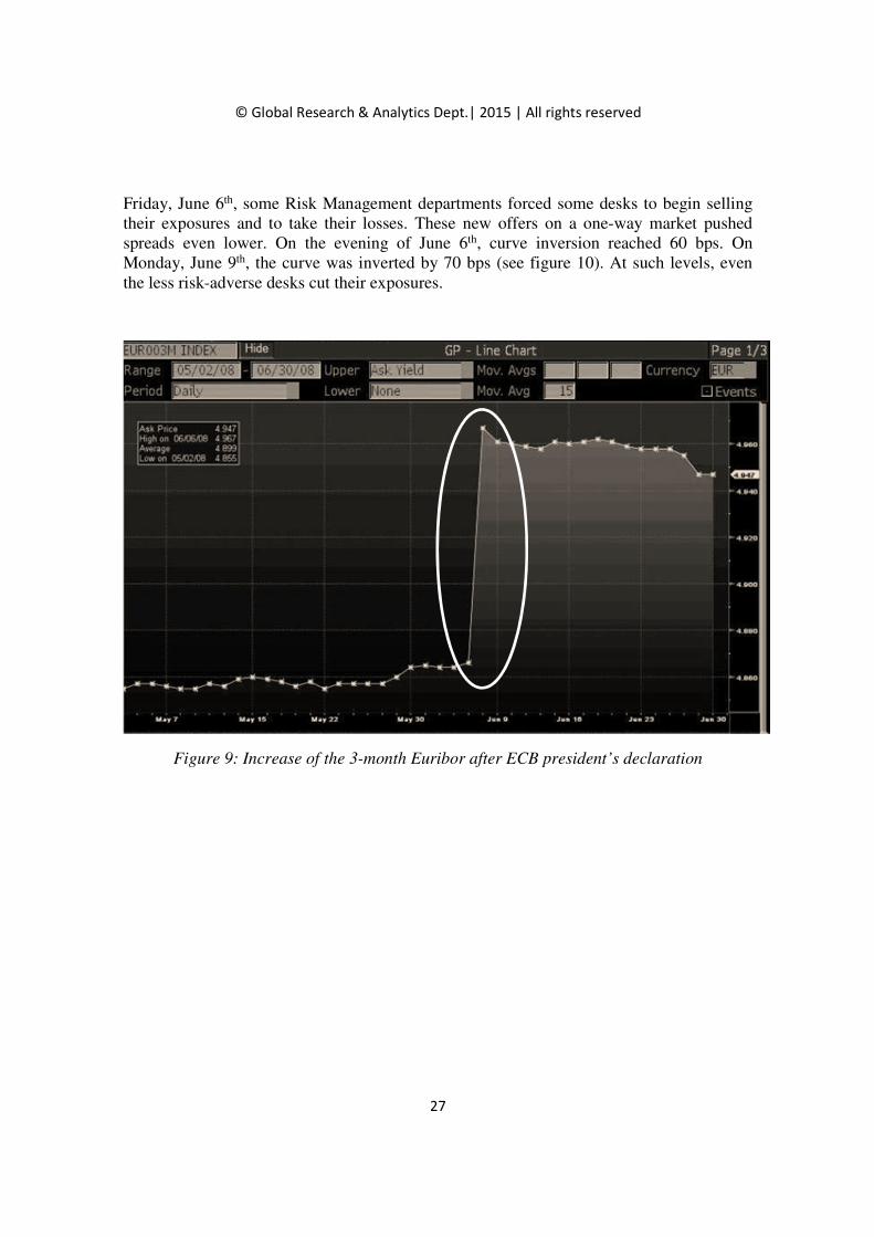
Immediately, markets went wild. Facing a highly probable rate increase in July, short rates climbed while long rates dropped (see on figure 9 the strong increase of 3-month Euribor). Structured desks were plunged into an extreme case scenario: in a few minutes’ time, their spread gamma and vega exposures reversed completely and they discovered that they were now strongly gamma-negative. The fall of spreads and these
gamma-negative exposures created significant positive delta-spread exposures: @ ≈ A∆ >0. All traders were long of the underlying, and no one wanted to buy spreads any more. Consequently bids on spreads disappeared and, mechanically, without any significant transaction, offers dropped. On the evening of June 5th, the curve was already inverted by 30 bps. In a parallel way, the important exposures of traders to the steepening of the curve began to cross their risk limits. The traders' dilemma was the following: would they stop losses and cut delta exposures by massively selling the spreads when the market was lower than it had ever been, or would they wait and keep their exposures, hoping for the market to recover soon, which could lead to far greater losses if the market kept falling? In the end, risk aversion took over as exposures to steepening reached unprecedented levels. On
3 Source: http://www.ecb.int/press/pressconf/2008/html/is080605.en.html 4 Source: http://www.ecb.int/press/pressconf/2008/html/is080605.en.html
© Global Research & Analytics Dept.| 2015 | All rights reserved
27
Friday, June 6th, some Risk Management departments forced some desks to begin selling their exposures and to take their losses. These new offers on a one-way market pushed spreads even lower. On the evening of June 6th, curve inversion reached 60 bps. On Monday, June 9th, the curve was inverted by 70 bps (see figure 10). At such levels, even the less risk-adverse desks cut their exposures.
Figure 9: Increase of the 3-month Euribor after ECB president’s declaration

© Global Research & Analytics Dept.| 2015 | All rights reserved
28
Figure 10: Evolution of the 30Y – 2Y spread after ECB president’s declaration
In the following days, a similar issue arose on spread vega exposures, as desks were extremely short. Short volatilities (3M2Y , 3M10Y , 3M30Y ) increased strongly after the ECB President 's announcement, as shown on figure 11:

© Global Research & Analytics Dept.| 2015 | All rights reserved
29
Figure 11: Evolution of the 3M2Y volatility after ECB president’s declaration
The same dilemma arose: cut the exposure by buying immediately or wait and hope for a recover. Again, Risk Management departments forced desks to cut most of the exposures and pushed volatilities higher, increasing losses.
Another strong impact of these market moves was indirect and arose from margin call effects: as the curve inverted, the fair value of the exotic spread-options in the portfolio rose rapidly, while the value of the hedges dropped. But the counterparties of the banks on spread-options were mainly corporates, and the collateral agreements that the banks had put in place with them did not require frequent margin calls. Therefore, the banks did not receive a lot of collateral from these counterparties. But the counterparties on hedges were mostly other banks, and the collateral agreements between banks were often more restrictive, requiring weekly or even daily margin calls. Soon the banks were required to post important amounts of collaterals.
In the following weeks and months, the EUR curve steepened again, but it was too late and exotic desks, who went back to delta-neutral positions when the spreads were at their lowest, did not profit from this return. Actually, they suffered more losses as they were still strongly gamma-negative. The final outcome was bad for everyone: for clients, who did not receive any coupons from the bank and suffered from strongly negative mark-to-market values, and for traders, who had not anticipated the inversion and were severely struck by this exotic risk they could neither hedge nor manage.

© Global Research & Analytics Dept.| 2015 | All rights reserved
30
4. The consequences - A basic illustration
If we come back to the simple case of a single digital option on spread as presented above, we can try to approximate the impact of such an extreme scenario (strong curve inversion).
We consider the case of a simple swap in which the bank pays on 1st December 2008 a payoff of 5% if EUR spread 30Y – 2Y ≥ 0 or 0% otherwise, the level of the EUR 30Y – 2Y spread being fixed on 1st September 2008. The notional is 10,000,000 Euros, and
the � coefficient used in the valuation is 10 bps.
Then the value of the digital option, given market data at the pricing date, can be calculated with the formula given above (formula (1), (2), (3) and (4)): on 1st June 2008 it is -247k EUR. The sensitivities of the swap are:
• @ = - 667,136 EUR,
• A = + 3,825 EUR and
• B = + 565 EUR.
Now we use the market data of 9th June 2008, when the curve inversion is at its peak. Then the value of the swap is -244k EUR, and sensitivities have changed to:
• @ = - 406,025 EUR,
• A = - 11,182 EUR and
• B = - 2,593 EUR.
The variation of value is positive (+ 3k EUR). However, one should keep in mind that the trader has hedged his delta and vega exposure on this product before 1st June 2008. He has bought and sold swaps in order to obtain an overall delta exposure of + 667 136 EUR, and swaptions in order to obtain a vega exposure of - 565 EUR. If we add to the variation of value of the product the variation of its hedges, we obtain the global impact on the portfolio value, which is - 2,267 EUR. If we extend this analysis, taking into account that most of the digital products sold by the banks had more than one coupon (typically those products pay quarterly coupons for 10 or 20 years), and taking into account the size of the portfolios held by banks (several billions of notional), the impact for a typical exotic book could reach a hundred million Euros or more. As a matter of fact, if we assume those products had an average maturity of 15 years (60 quarters) and their cumulated notional in
an average exotic book was 10 billion Euros, the loss would be around 1 000 × 60 ×
2 267 ≈ 136 million Euros.
Beyond the P&L effects described above, some key risk drivers were also impacted:
• indirectly by increasing the regulatory capital required under market risk (increase in Basel II VaR), as the risk positions of the exotic books increased strongly,
• directly by increasing drastically the funding risk of the bank (margin call effects)
• virtually if some internal short-term liquidity ratios had existed at that time (Liquidity Coverage Ratio in particular)

© Global Research & Analytics Dept.| 2015 | All rights reserved
31
5. A problematic shared with other asset classes - Focus on
commodities
Discontinuous payoffs popularity has spread across all financial asset classes and
soon enough volumes have picked up and payoffs have become more complex, driving
investment banks to find new sources of diversification and enticing risk (or income)
seeking investors into new product families. Whatever the asset class, the risks involved in
trading these discontinuous payoffs are similar, as not directly related to the underlying
asset: gamma and vega flip sign at the barrier, delta magnitude is maximum at the barrier.
Geopolitical, climatic, transportation or warehousing constraints can have drastic
impacts on commodity products supply & demand, and therefore sudden increase in
volatility on these markets is somewhat common. A commodity investor willing to take
advantage of a high volatility environment while receiving income with some protection
would be directed to discontinuous payoff products.
Indeed, income products are popular among Private bank investors as they either
provide a regular coupon or an upfront receivable coupled with an upside exposure to the
underlying commodity. In order to finance this coupon, banks usually package a hedging
instrument on the downside, usually with a barrier to offer some buffer protection to the
investor and therefore limit the potential loss. Alternatively, investor can just sell the
option to the investment bank in order to collect the premium and expect the underlying
price to maintain above the barrier. These types of products are very popular among private
bank investors as they offer decent return, are very competitively priced and payoff stay
relatively simple.
Let’s take an example on that kind of structure.
Say an investor has a flat-to-bullish view that gold will maintain within the 1200-
1250 (currently at $1,225 per troy ounce) range in the next year, and wants to monetize it.
He thinks about selling an option on gold that would provide him with some upfront cash
while being protected in case his view was erroneous and gold drops by up to 15%. The
option that fits these investor requirements would be a down-and-in put on gold with strike
equal to the spot market ($1,225 per troy ounce) and barrier price at 85% of current spot
($1,041.25 per troy ounce) with a maturity of 1 year. Another decision to be made is on the
observation dates: should it be with continuous observation, daily discrete, periodically
(like quarterly) or at expiry. This choice would have a great importance since the more
observation dates you have, the more chances you have to cross the barrier and activate the
put, hence a pricier option. So the investor would arbitrate between maximizing his
© Global Research & Analytics Dept.| 2015 | All rights reserved
32
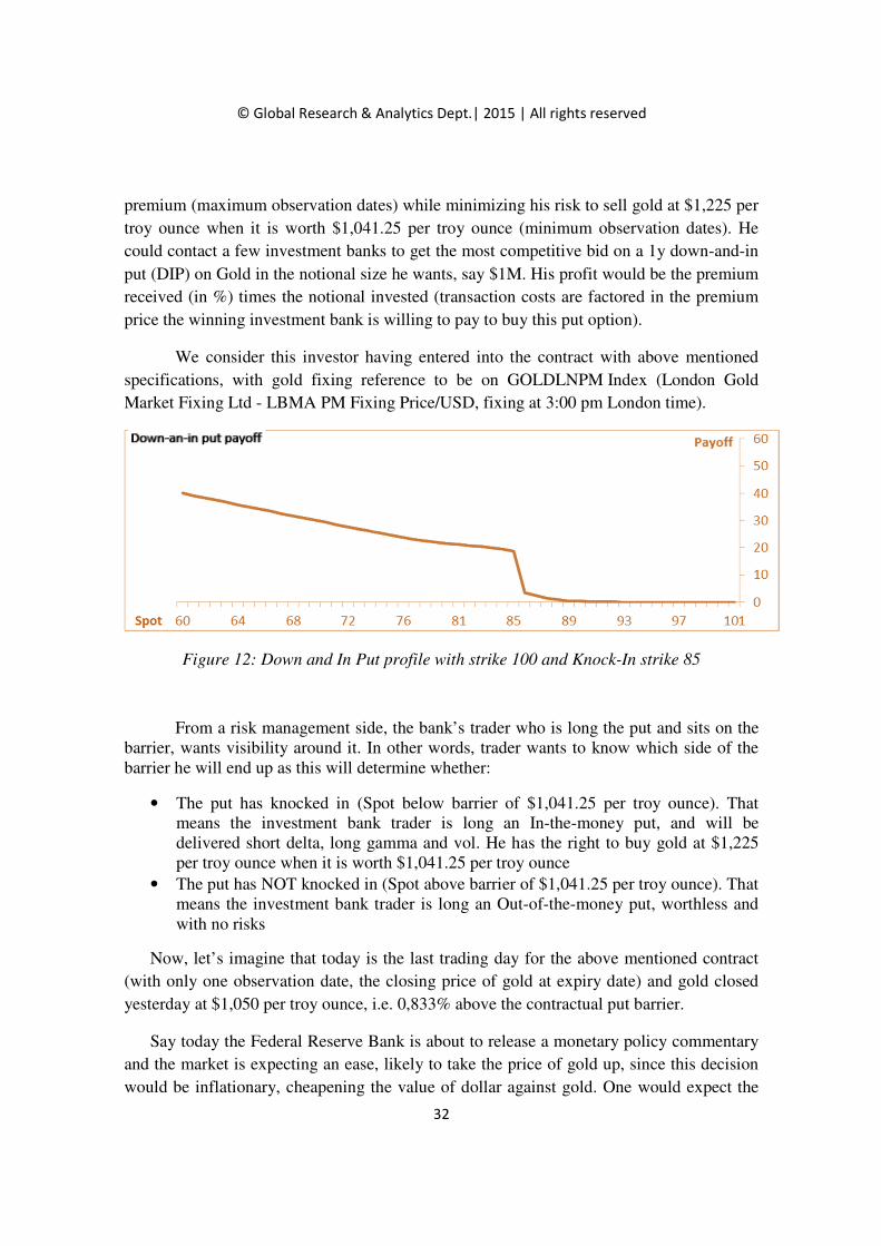
premium (maximum observation dates) while minimizing his risk to sell gold at $1,225 per
troy ounce when it is worth $1,041.25 per troy ounce (minimum observation dates). He
could contact a few investment banks to get the most competitive bid on a 1y down-and-in
put (DIP) on Gold in the notional size he wants, say $1M. His profit would be the premium
received (in %) times the notional invested (transaction costs are factored in the premium
price the winning investment bank is willing to pay to buy this put option).
We consider this investor having entered into the contract with above mentioned
specifications, with gold fixing reference to be on GOLDLNPM Index (London Gold
Market Fixing Ltd - LBMA PM Fixing Price/USD, fixing at 3:00 pm London time).
Figure 12: Down and In Put profile with strike 100 and Knock-In strike 85
From a risk management side, the bank’s trader who is long the put and sits on the barrier, wants visibility around it. In other words, trader wants to know which side of the barrier he will end up as this will determine whether:
• The put has knocked in (Spot below barrier of $1,041.25 per troy ounce). That means the investment bank trader is long an In-the-money put, and will be delivered short delta, long gamma and vol. He has the right to buy gold at $1,225 per troy ounce when it is worth $1,041.25 per troy ounce
• The put has NOT knocked in (Spot above barrier of $1,041.25 per troy ounce). That means the investment bank trader is long an Out-of-the-money put, worthless and with no risks
Now, let’s imagine that today is the last trading day for the above mentioned contract
(with only one observation date, the closing price of gold at expiry date) and gold closed
yesterday at $1,050 per troy ounce, i.e. 0,833% above the contractual put barrier.
Say today the Federal Reserve Bank is about to release a monetary policy commentary
and the market is expecting an ease, likely to take the price of gold up, since this decision
would be inflationary, cheapening the value of dollar against gold. One would expect the
© Global Research & Analytics Dept.| 2015 | All rights reserved
33
market to be nervous with a bias on the upside, many actors placing some stop losses on
the downside in case the FED base rate stays unchanged (or FED takes a hawkish stand).
The gold trading day would be very volatile, with gold price going below and above
$1,041.25 per troy ounce a few times (but no put activation since the official observation
price is the closing price). Understandably, both the investment bank trader and the private
bank investor are nervous as the payoff and risks for them are binary: all or nothing. The
trader would be either short gold for $1M or nothing. Alternatively, the investor would
have to pay the investment bank trader $1M x Max(Spot-Strike;0). Decision for the
investment bank trader is then ultimately: how can I maximize my profit while still protect
myself against a rise in gold price? Question which comes down to: shall I re-hedge my
delta, as he cannot predict with certainty whether the option will be exercised or not?
For instance, say GOLDLNPM trades at $1,043 per troy ounce at 2:58 pm. The DIP is
out of the money and therefore will expire worthless at this price. At 2:59 pm,
GOLDLNPM trades at $1,040 per troy ounce and the DIP is now in the money, and the
terms of the contract will favor an automatic exercise of the put option. At that time the
trader would flatten his short delta (that would be inherited from the put exercise) buy
buying $1M gold at $1,040 per troy ounce. Twenty seconds before the close, GOLDLNPM
moves back to $1,042 per troy ounce, DIP is out of the money and the trader must know
sell back his $1M gold delta just acquired….
Bullion products, namely gold and silver, have experienced very high volatility several
times since 2008. Sharp and sudden movements have pushed these barrier products near or
breach across their barrier. As a result, many investors as well as banks faced sudden losses
• Investors saw their investment mark-to-market drop suddenly (barrier [nearly]
breach bringing their short put position in the money). That means investment
banks became shorter as the long puts (nearly) activated. Long hedges on the
exchange received margin call since their value dropped and banks needed to post
initial margin for new longs needed to hedge the short position inherited from the
drop in price of gold. That sparked a rush for cash liquidity or high quality
collateral.
• Banks not applying conservative risk management techniques (like barrier bending)
had difficulties in hedging rapidly and adequately. Indeed, they had more difficulty
in monitoring the breach (no early warning as their risks were not smoothen) and
they experienced a binary switch in risks.
This was particularly telling mid-April 2013 as shown by the historical prices graph below.
Indeed, on April 15th, Gold plunged the most in 33 years amid record-high trading as an
unexpected slowdown in China’s economic expansion sparked a commodity selloff from
investors, concerned that more cash will be needed to cover position.

© Global Research & Analytics Dept.| 2015 | All rights reserved
34
Figure 13: Evolution of spot Gold in April 2013 amid fears on China’s economic slowdown
6. It could have been avoided...
Going back to the case of interest rate structured desks, the output was bad: the final
losses for most interest rate structured derivatives desks were huge, reaching hundreds of
millions of Euros. Facing such a disaster, one can only be surprised by the almost complete
lack of anticipation from traders: these losses could have been avoided. Such an inversion
was indeed a brand new move for the EUR curve, but it had already happened on other
curves, like the USD curve. Therefore it should not have been such a surprise for interest
rates desks to see the EUR curve invert. Besides, most structured desks frequently run
stress-tests on their book simulating the impact of predefined market scenarios (on a daily
or weekly basis), some of them being based on a strong decrease of spreads. The results of
these scenarios should have warned traders and/or risk departments that they were on the
edge of massive losses. Yet it seems that no one had considered these scenarios seriously.
There were solutions to hedge this risk, as the curve flattened slowly at first, and even
stayed flat for a few days. Meanwhile, the traders could have put in place some macro-
hedging strategies. For instance, when spreads were closing to zero, it was easy to enter a
strong curve flattening delta position (i.e. @ < 0). Thus in case of an inversion this negative
delta exposure would have given a strong profit: @ × ∆ ≫ 0. Gains on this exposure could
have offset losses on the gamma position of exotics. This strategy was rather cheap
compared to the losses that it could prevent.

© Global Research & Analytics Dept.| 2015 | All rights reserved
35
Going back to the calculation framework of the previous section, we can see that a
flattening position should be around 1.4 million Euros of delta in order to ensure a 100
million Euros profit during the inversion. Such an exposure could be obtained through a
30y receiver swap with a notional of 950 million euros, and a 2y payer swap with a
notional of 9.78 billion Euros. These notionals may seem big, but a trader who had seen the
danger soon enough would have at least a few days to put this exposure in place by smaller
tranches, with a limited impact on market prices and without suffering from important
transaction costs. By splitting these swaps in 20 pieces, transaction costs could have been
reduced to 1 or 2bps, i.e. a total of 1.4 to 2.8 million Euros. This is a small amount of
money, compared to the avoided losses.
Risk and control departments have also failed in this particular case, mostly because
they did not use the right indicators. As we have shown above, in this particular case the
risk could not be seen in the greeks of the portfolio, which was the main indicator used by
risk departments.
Even in VaR models, the danger was not clearly visible. Most banks use Monte-Carlo
schemes and random market scenarios in order to calculate their VaR, and clearly a
scenario in which the 30Y – 2Y spread dropped by almost 70bps in only 2 days was
perceived as extremely improbable then (or even impossible) and could not impact a 99.9%
VaR.
Different indicators could have raised a hint to risk departments. We have already
mentioned stress-tests (although, to be fair, it is highly improbable that any bank would
have considered a 70bps inversion scenario in its stress-tests before it happened…). But
even a 20 or 30bps inversion scenario could have shown risk departments that a huge risk
was hidden in the portfolios. More precisely, risk departments could also use a mapping of
every digital and barrier option of the portfolio and their strikes, in order to identify points
of accumulation. They could have defined exposure limits on a given strike, in terms of
notional exposures or greeks. These solutions are examined in details in section 7 of this
paper.
But the truth is, most structured desks were completely taken by surprise by the
inversion, which sheds light on the risk management practices inside banks' market
activities and their deficiencies. Besides, this episode also reveals an inner weakness of
exotic activities: a concentration of unhedgeable risks is a necessary consequence of this
business. Practically, when a product is popular, it is massively sold by banks to their
clients, leading to an uncomfortable situation where all banks accumulate the same risk
concentration. When market evolution triggers the realization of the risk, all banks turn to
the market to get rid of their products and the huge volume on the offer side of this one-
way market makes prices plunge deeper.

© Global Research & Analytics Dept.| 2015 | All rights reserved
36
7. Efficient risk management techniques
Discontinuity in barrier deals payoff together with high volatility in underlying asset
moves, requires that traders use effective techniques to both smoothen their daily risk
management and P&L volatility and plan their strike management. The following sections
aim to give guidance on the use of a few techniques to manage discontinuity risk: barrier
bending, concentration and limit risk management and stress testing.
A. Bending strategies
One can use dynamic hedges (delta hedging) or static hedges (use other options), but
this proves costly and not always efficient. A powerful way to manage risks around the
barrier is to “bend” it, namely with the use of put/call spreads, in order to limit barrier
discontinuity risk at observation date(s). This technique has already been mentioned above,
as it is widespread among structured derivatives desks. The objective for the bank’s trader
is to gradually and conservatively represent risks. Indeed, bank’s trader will gradually
come in the money from the barrier, thanks to a risk booking where the put will activate
below the contractual strike. Therefore, it is easier for the trader to manage sensitivities
around the barrier as the magnitude of the risk is more manageable and gradual compared
to a binary risk with the contractual booking (cf. Figure 2). This conservative risk
management technique is not directly impacting the financial product final payoff. Indeed,
the risk booking on bank’s side is not impacting the terms of the contract and any
underlying below the contractual barrier, say X, will activate the put even if the underlying
fixes between X and the risk booking barrier. On the other hand, if the trader used a put
with a barrier at 98% of X, he will be in the money thanks to a bigger drop in the
underlying. If 98% X < X, then Put (98% X) < Put(X). Therefore, the value the investor is
expected to receive or pay at contract maturity is greater than the risk-managed / bended
value. However, this would reflect mechanically in the daily valuations provided to bank’s
client as valuations provided to clients on a daily basis come from the Front Office risk
management system. This is also a “mid” value from which the bank’s trader would not be
willing to unwind the position: indeed, he is usually long the put and unwinding this
position at the risk managed mid would generate losses. It is therefore a challenge to show
a market to investors that is shifted from the FO systems. The usage in many investment
banks though is to give back one third of the bending value taken upfront to the client
when unwinding.

© Global Research & Analytics Dept.| 2015 | All rights reserved
37
For instance, say an investment bank buys a down-and-in-put with an underlying strike
price of 100 and a barrier at underlying price of 85, from a private bank (acting as an agent
for a private investor) for a theoretical value of 15%. The investment bank trader would be
willing to pay 14.5% to buy this option, as he would factor the conservative barrier
bending in the risk management cost to trade. In other words, the trader would enter this
product in his books at a lower value than what he would have done, had he not “bent” the
barrier. The investment bank trader, who is long the put option, would be in the money at a
lower price (say at underlying price 83.3) than where he would have been without the bend,
85: the put option is worth less to him and this view is therefore conservative. Investment
bank’s trader put will go in the money BELOW bent barrier strike (instead of AT
contractual barrier strike). The trader put will deliver sensitivities BEFORE the barrier is
touched, which serves 3 purposes:
1. Alert the trader the barrier is near breach 2. Prepare hedging strategy 3. Conservatively risk manage (Investment bank’s trader can expect some windfall)
Bending practice aims to smoothen greeks and mitigate/spread digital (or pin) risk around the barrier. Trading desks use different approaches to achieve this:
• In the past, these included namely: o Booking offsetting linear rebates (to a certain theta limit the desk/market
risk management felt comfortable to bear): offsetting risk management cashflows that activate as soon as the underlying nears the barrier
o Rainbow weights: assets are bent depending on their liquidity/standard deviation
o Booking different strikes or call spreads o Other ways to over-hedge (offsetting options in larger size than needed)
• Nowadays, trading desks apply outright bends (see below) o Changing strikes/barriers in the risk booking o Approximate digitals as call spreads
B. Examples of bending strategies
The below section presents different ways of bending a barrier that prove useful in a set of situations. Note that these ways can be combined for a maximum effect and command.

© Global Research & Analytics Dept.| 2015 | All rights reserved
38
C. Manage risk concentration and limits
A risk manager in an investment bank monitors digital risks (size, barrier, potential early unwind/redemption…) by observation dates and barrier strikes to avoid too much concentration on some barrier strike and/or underlying, and to allow effective risk management by the trading desk and other departments (Risks, Middle Office, Quants) to take precautionary measures.
1. Monitoring observation dates and distance to barrier
Observation dates for a barrier can be continuous (during trading hours), discrete daily or at expiry. That means the problematic risk management can occur on these dates where the underlying price of the financial product will be compared to the payoff conditions detailed in the contract binding the investment bank to the investor.
A daily dashboard can be submitted to the trading desk by risk managers and/or middle office, with a specific “urgency” time window. Aim for the trader is to see prospectively as and when a problematic risk management would arise. A simple and effective way to risk manage barrier products is to maintain a dynamic matrix with a double entry:
© Global Research & Analytics Dept.| 2015 | All rights reserved
39
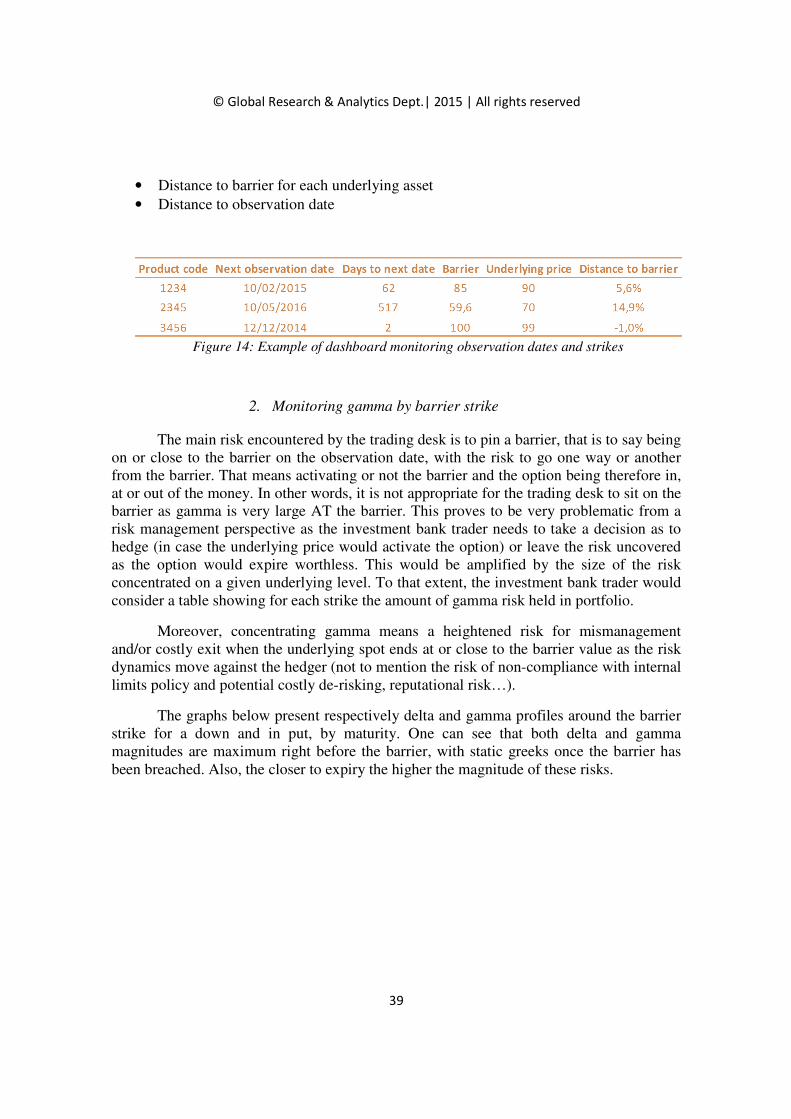
• Distance to barrier for each underlying asset
• Distance to observation date
Figure 14: Example of dashboard monitoring observation dates and strikes
2. Monitoring gamma by barrier strike
The main risk encountered by the trading desk is to pin a barrier, that is to say being on or close to the barrier on the observation date, with the risk to go one way or another from the barrier. That means activating or not the barrier and the option being therefore in, at or out of the money. In other words, it is not appropriate for the trading desk to sit on the barrier as gamma is very large AT the barrier. This proves to be very problematic from a risk management perspective as the investment bank trader needs to take a decision as to hedge (in case the underlying price would activate the option) or leave the risk uncovered as the option would expire worthless. This would be amplified by the size of the risk concentrated on a given underlying level. To that extent, the investment bank trader would consider a table showing for each strike the amount of gamma risk held in portfolio.
Moreover, concentrating gamma means a heightened risk for mismanagement and/or costly exit when the underlying spot ends at or close to the barrier value as the risk dynamics move against the hedger (not to mention the risk of non-compliance with internal limits policy and potential costly de-risking, reputational risk…).
The graphs below present respectively delta and gamma profiles around the barrier strike for a down and in put, by maturity. One can see that both delta and gamma magnitudes are maximum right before the barrier, with static greeks once the barrier has been breached. Also, the closer to expiry the higher the magnitude of these risks.

© Global Research & Analytics Dept.| 2015 | All rights reserved
40
Figure 15: Delta & Gamma profiles for down and in put
D. Stress testing
Running regular stress tests with appropriately chosen scenarios specifically on the
book comprised of barrier options can also help identify potential problematic situations
and help anticipate exit/hedging and capture extreme events that a regular VaR would not.
Specific scenarios can be built to suit the specificities of the underlying assets, offering
more granularity in the input as well as results. These “targeted” stress tests shall be quick
to design and implement, thanks to the expected limited number of positions in the book,
the consistency in the underlying set and similarities in payoffs. Risk management
departments shall set up an agile stress test platform that can be tailor-made to a specific
market environment and/or stricter risk appetite while maintaining a robust risk
management oversight on traders’ activities.
“What if” scenarios would therefore reveal potential market conditions under which
the investment bank trader would experience turbulences on the risk management of the
option position. An example could be the stress of a portfolio of gold digital options with a
global economic slowdown on a 2-year horizon, with a drop in China industrial output:
running this scenario could help reveal which trades would breach or come close to the
barrier. Consequently, appropriate barrier bending could be put in place to manage
effectively the risks involved.
© Global Research & Analytics Dept.| 2015 | All rights reserved
41
8. Conclusion
Risk management techniques within banks have become more and more sophisticated in
order to cope with products and underlying complexity, bearing very dynamic risks. On top
of helping banks better manage their exotic risks and P&L volatility, risk management
techniques have proven to be cost efficient tools in adverse market conditions. This
deployment is also another answer to recommendations from supervisory authorities on a
better management of market risk and liquidity. In this context, the present white paper
provides clarification on past situations where banks experienced unexpected losses on
portfolios that were deemed under control. Moreover, this study gives an introduction to
some risk management techniques for managing discontinuity risk and limit losses, with
specific examples on interest rate and commodity underlyings.

© Global Research & Analytics Dept.| 2015 | All rights reserved
42
Bibliography
Brigo, D. and Mercurio, F. – Springer – 2006, Interest Rate Models - Theory and Practice - With
Smile, Inflation and Credit.
Iwasawa, K. (2001), Analytic Formula for the European Normal Black Scholes Formula
European Central Bank (5th June 2008), new monetary policy press conference http://www.ecb.int/press/pressconf/2008/html/is080605.en.html
Christofferson, P., and S. GonCalves (2005): “Estimation risk in financial risk management,”
Journal of Risk, 7, 1–28.
Cont, R., R. Deguest, and G. Scandolo (2010): “Robustness and sen- sitivity analysis of risk
measurement procedures,” Quantitative finance, 10, 593–606.
Engle, R. (2002): “Dynamic conditional correlation: A simple class of mul- tivariate generalized
autoregressive conditional heteroskedasticity models,” Journal of Buisiness and Economic
Statistics, 20, 236–249.
Jorion, P. (2006): “Value at Risk,” McGraw-Hill, 3rd edn.
Kashyap, A., and J. Stein (2004): “Cyclical Implications of the Basel II Capital Standards,”
Federal Reserve Bank of Chicago Economic Perspectives, 20.
Lehar, A. (2005): “Measuring systemic risk: A risk management approach,”Journal of Banking
and Finance, 29, 2577–2603.
Nieto, M., and E. Ruiz (2009): “Measuring financial risk: Comparison of alternative procedures
to estimates VaR and ES,” Universidad Carlos III de Madirid Working paper.(2010): “Bootstrap
prediction intervals for VAR and ES in the context of GARCH models,” Universidad Carlos III
de Madirid Working paper.
Pascual, L., M. Nieto, and E. Ruiz (2006): “Bootstrap prediction for re- turns and volatilities in
GARCH models,” Computational Statistics and Data Analysis, 50, 2293–2312.
Carol ALEXANDER – John Wiley & Sons Ltd – 2008. Market Risk Analysis – Volume IV – Value-at-Risk Models,
John C. HULL – Prentice Hall – 2007, Options, futures et autres actifs dérivés,.
Carol ALEXANDER – John Wiley & Sons Ltd – 2001. Market Models, A Guide to Financial
Data Analysis –.
ARTZNER, DELBAEN, EBER & HEATH - Coherent Measures of Risk – Mathematical Finance – 1999.
Philip BEST , Implementing Value at Risk –– John Wiley & Sons Ltd – 1998.

© Global Research & Analytics Dept.| 2014 | All rights reserved
0
.
Related Documents


