Risk, jumps, and diversification

Risk, jumps, and diversification

Tim Bollersleva,1, Tzuo Hann Lawb, George Tauchena,�

aDepartment of Economics, Duke University, Durham, NC 27708-0097, USAb76, Lorong 7, Taman Suria, 34000 Taiping, Malaysia

Available online 13 February 2008

Abstract

We test for price discontinuities, or jumps, in a panel of high-frequency intraday stock returns and an equiweighted

index constructed from the same stocks. Using a new test for common jumps that explicitly utilizes the cross-covariance

structure in the returns to identify non-diversifiable jumps, we find strong evidence for many modest-sized, yet highly

significant, cojumps that simply pass through standard jump detection statistics when applied on a stock-by-stock basis.

Our results are further corroborated by a striking within-day pattern in the significant cojumps, with a sharp peak at the

time of regularly scheduled macroeconomic news announcements.

r 2008 Published by Elsevier B.V.

JEL classification: C12; C22; C32; G12; G14

Keywords: Jump-diffusions; Stock returns; Diversification; Tests for jumps; Cojumps; High-frequency data; Bipower variation

1. Introduction

We examine the relationship between jumps in individual stocks and jumps in an aggregate market index.Several studies have recently presented strong non-parametric high-frequency data-based empirical evidencein favor of jumps in financial asset prices, thus discrediting the classical continuous time paradigm withcontinuous sample price paths in favor of one with jump discontinuities.2 The tests that we implement herefurther corroborate this evidence for the presence of jumps at both the individual stock and aggregate marketlevel. Of particular interest, however, are the contrasts between the outcome of tests for jumps conducted atthe level of the individual stocks and the level of the index. Jumps in individual stocks can be generated byeither stock-specific news or common market-level news. Meanwhile, from basic portfolio theory one mightexpect that jumps in a well-diversified index should only be generated by market-level news that inducescojumps across many stocks. Below, we formalize these ideas and develop a new test for cojumps motivated

www.elsevier.com/locate/jeconom

0304 4076/$ f t tt r 2008 P bli h d b El i B V

�Corresponding author. Tel.: +1 919 660 1812.

E-mail addresses: [email protected] (T. Bollerslev), [email protected] (T.H. Law), [email protected] (G. Tauchen).1Tel.: + 1 919 660 1846.2Empirical studies and new statistical procedures include the work of Ait-Sahalia and Jacod (2008), Andersen et al. (2007b), Barndorff-

Nielsen and Shephard (2004), Fan and Wang (2006), Huang and Tauchen (2005), Jiang and Oomen (2006), Lee and Mykland (2008), and

Mancini (2004).

directly by these observations. As such, the test explicitly reflects all of the cross-covariances within a largepanel of high-frequency returns.

Jumps are clearly of importance for asset allocation and risk management. A risk averse investor might beexpected to shun investments with sharp unforeseeable movements. As an example of a jump, consider Fig. 1,which depicts the price of Proctor and Gamble (PG) on August 3, 2004 sampled once every 30 s. There is asharp discontinuity in the evolution of the prices a little after 11 am, where PG gains about 30 cents over aperiod of just 2min. Jumps like that are of great importance for standard arbitrage-based arguments andderivatives pricing in particular, as the effect cannot readily be hedged by a portfolio of the underlying asset,cash, and other derivatives.3

Of course, not all jumps are as sharply ex post identifiable as that shown in Fig. 1, so that a formal statisticalmethodology for identifying jumps is needed. In the results reported on below, we start with a univariateanalysis of stock-by-stock jump tests based on the seminal work by Barndorff-Nielsen and Shephard (2004)(BN–S). The BN–S theory provides a convenient non-parametric framework for measuring the relativecontribution of jumps to total return variation and for classifying days on which jumps have or have notoccurred.

Our empirical investigation is based on high-frequency intraday returns for a sample of forty large-cap U.S.stocks and the corresponding equiweighted index of these same stocks over the 2001–2005 sample period.Consistent with previous empirical results, we find strong evidence for the presence of jumps in each of theindividual stock price series as well as the aggregate index. Standard computations also indicate about 15–25large jumps for each of the individual stocks scattered randomly across the five-year sample, with jumpsaccounting for 12% of the total variation on average. In contrast, for the aggregate index there are only sevenhighly significant large jumps across the whole sample, and jumps as a whole account for just about 9% of thetotal return variation. Although these specific numbers obviously rely on our use of the popularBN–S procedure for identifying jumps, the same basic findings of more frequent and larger sized jumps forthe individual stocks compared to the index is entirely consistent with the limited empirical evidence based onthe univariate threshold-type statistic recently reported in Lee and Mykland (2008).

ARTICLE IN PRESS

10am 11am 12pm 1pm 2pm 3pm 4pm53

53.2

53.4

53.6

53.8

54

54.2

54.4

Time of Day

Pric

e, $

Fig. 1. Price of PG sampled every 30 s on August 3, 2004.

3More formally, the effect of a jump on the price of a derivative is locally nonlinear and thereby cannot be neutralized by holding an ex

ante-determined portfolio of other assets.

T. Bollerslev et al. / Journal of Econometrics 144 (2008) 234–256 235

The fact that the data reveal a less important role for jumps in the index than in each of its components isnot all surprising, since the idiosyncratic jumps should be diversified away in the aggregate portfolio. At thesame time, however, there is at best a very weak positive association between the significant jumps in eachof the individual stocks and the jumps in the index. The BN–S jump detection procedure relies on a dailyz-statistic, with large positive values of the statistic discrediting the null hypothesis of no jumps on that day.We find the z-statistics for the individual stocks to be essentially uncorrelated with the z-statistics for the index,despite the fact that most of the individual stocks have b’s close to unity with respect to the index.

As one might conjecture, this low degree of association appears to be due to the large amount ofidiosyncratic noise in individual returns. This noise masks the cojumps, making them nearly undetectable atthe level of the individual return. To circumvent this problem, we develop a new cojump test applicable tosituations involving large panels of high-frequency returns.4 Using this new test statistic we find strongevidence for many modest-sized common jumps that simply pass through the standard univariate jumpdetection statistic, while they appear highly significant in the cross-section based on the new cojumpidentification procedure.

As noted by Andersen et al. (2007b), Barndorff-Nielsen and Shephard (2006), Eraker et al. (2003), andHuang and Tauchen (2005) among others, many, although not all, of the statistically significant jumps inaggregate stock indexes coincide with macroeconomic news announcements and other ex post readilyidentifiable broad-based economic news which similarly impact financial markets in a systematic fashion.5

While macroeconomic events obviously also affect individual firms, individual stock prices are also affected bysudden unexpected firm-specific information that can force an abrupt revaluation of the firms’ stock.6 Ourresults suggest that firm-specific news events are indeed the dominant effect of the two in terms of theirimmediate price impact at the individual stock level, and only by properly considering the cross-section ofreturns do the non-diversifiable cojumps become visible in a formal statistical sense. These results are furthercorroborated by our findings of strong intraday patterns in the importance of jumps across the day, with thepeak in the pattern for the aggregate index closely aligned with the time of the release of regularly schedulednews announcements.

The rest of the paper proceeds as follows. Section 2 outlines the basic second-moment theory that underliesmost of the recent univariate high-frequency data-based jump detection work, along with the relevantmultivariate large-panel extensions. Section 3 briefly reviews the standard univariate (BN–S) jump test anddevelops our new test for cojumps based on the multivariate extensions from the preceding section. Section 4discusses the high-frequency data and sampling schemes underlying our empirical analysis, with some of thedetails relegated to Data Appendix. Section 5 presents our main empirical findings, while Section 6 concludeswith a few final remarks.

2. Generalized quadratic variation theory

2.1. Univariate second-moment variation measures

We start by considering the ith log-price process piðtÞ from a collection of n processes fpiðtÞgni¼1 evolving incontinuous time. We assume that piðtÞ evolves as

dpiðtÞ ¼ miðtÞdtþ siðtÞdwiðtÞ þ dLi;JðtÞ, (1)

where miðtÞ and siðtÞ refer to the drift and local volatility, respectively, wiðtÞ is a standard Brownian motion,and Li;JðtÞ is a pure jump Levy process.7 A common modeling assumption for the Levy process is thecompound Poisson process, or rare jump process, where the jump intensity is constant and the jump sizes are

ARTICLE IN PRESS

4Alternative statistical procedures for identifying common jump arrivals in pairs of returns have recently been developed by Jacod and

Todorov (2007) and Gobbi and Mancini (2007).5Notable examples include the monthly employment report, FED interest rate changes, oil prices, legislative alterations, and security

concerns.6For instance, lawsuits against a cigarette company, announcements of war for a defense company, or legislation of privacy issues for an

Internet search engine.7This particular notation is adopted from Basawa and Brockwell (1982).

T. Bollerslev et al. / Journal of Econometrics 144 (2008) 234–256236

independent and identically distributed. Throughout the paper we adopt the timing convention that one time-unit corresponds to a trading day, so that fpiðt� 1þ sÞgs2½0;1� represents the continuous log-price record overtrading day t, where the integer values t ¼ 1; 2; 3; . . . coincide with the end of the day.

In practice the price process is only available at a finite number of points in time. Let M þ 1 denote thenumber of equidistant price observations each day; i.e., piðt� 1Þ; piðt� 1þ 1=MÞ; . . . ; piðtÞ. The jth within-dayreturn is then defined by

ri;t;j ¼ pi t� 1þ j

M

� �� pi t� 1þ j � 1

M

� �; j ¼ 1; 2; . . . ;M, (2)

for a total of M returns per day.As discussed at length in, e.g., Andersen et al. (2008), the realized variance

RVi;t ¼XMj¼1

r2i;t;j (3)

provides a natural measure of the daily ex post variation. In particular, it is well known that for increasinglyfiner sampling frequencies, or M ! 1, RVi;t consistently estimates the total variation comprised of theintegrated variance plus the sum of the squared jumps

limM!1

RVi;t ¼Z t

t�1

s2i ðsÞdsþXNi;t

k¼1

k2i;t;k, (4)

where Ni;t denotes the number of within-day jumps on day t, and ki;t;k refer to the size of the kth such jump.In order to separately measure the two components that make up the total variation in (4), Barndorff-

Nielsen and Shephard (2004) and Barndorff-Nielsen et al. (2005) first proposed the so-called bipower variation

measure

BVi;t ¼ m�21

M

M � 1

� �XMj¼2

jri;t;j�1jjri;t;jj, (5)

where m1 ¼ffiffiffiffiffiffiffiffi2=p

p� 0:7979. Under reasonable assumptions, it follows that

limM!1

BVi;t ¼Z t

t�1

s2i ðsÞds, (6)

so that BVi;t consistently estimates the integrated variance for the ith price process, even in the presence ofjumps. Thus, as such the contribution to the total variation coming from jumps may be estimated byRVi;t � BVi;t, or the relative jump measure advocated by Huang and Tauchen (2005),8

RJi;t ¼RVi;t � BVi;t

RVi;t. (7)

It follows that in the limit asM ! 1, RJt40 only on days for which there are at least one jump, although forfinite M sampling variation can occasionally result in RJi;to0.

2.2. A portfolio-theoretic multivariate extension

The preceding subsection lays out the by now fairly standard univariate second-moment variation theory.However, from the point of view of financial economics, and in particular portfolio theory, we are generallymore interested in the behavior of a large ensemble of stock prices and returns. For a particular stock, say theith, the realized bipower variation BVi;t in (5) measures the combined common and idiosyncratic componentsof the continuous part of the total daily variation, while the realized variance RVi;t in (3) measures this plus thecontributions of both common jumps and idiosyncratic jumps. For a large portfolio that is well diversified in

ARTICLE IN PRESS

8An equivalent ratio statistic, �RJi;t, was proposed and studied independently by Barndorff-Nielsen and Shephard (2006).


the sense of the Arbitrage Pricing Theory, one might expect that the idiosyncratic jumps are diversified awayand only the common, or cojumps remain. This indeed turns out to be the case. For simplicity, we onlyconsider an equiweighted portfolio, but the arguments below hold with equal force for any well-diversifiedportfolio; there would just be the notational nuisance of including the portfolio weights in the proper places inthe formulas.

Consider the jth within-day return on an equiweighted portfolio of n stocks

rEQW;t;j ¼1

n

Xni¼1

ri;t;j.

Extending the arguments for the individual stocks with the same logic underlying equations (4) and (6), therealized variation for the EQW portfolio must satisfy

RVEQW;t ¼XMj¼1

1

n

Xni¼1

ri;t;j

!2

�!M!1 1

n2

Xni¼1

Z t

t�1

s2i ðsÞdsþ1

n2

Xni¼1

Xn‘¼1;‘ai

Z t

t�1

siðsÞs‘ðsÞds

þ 1

n2

Xni¼1

XNi;t

k¼1

k2i;t;k þ1

n2

Xni¼1

Xn‘¼1;‘ai

XN�t

k¼1

ki;t;kk‘;t;k,

where the last sum only includes the N�t jumps (a random number) that occur simultaneously across all n

stocks. Similarly,

BVEQW;t ¼ m�21

M

M � 1

� �XMj¼2

1

n

Xni¼1

ri;t;j�1

�� 1

n

Xni¼1

ri;t;j

��

�!M!1 1

n2

Xni¼1

Z t

t�1

s2i ðsÞdsþ1

n2

Xni¼1

Xn‘¼1;‘ai

Z t

t�1

siðsÞs‘ðsÞds.

Thus, it follows readily that

RVEQW;t � BVEQW;t �!M!1 1

n2

Xni¼1

XNt;i

k¼1

k2i;t;k þ1

n2

Xni¼1

Xn‘¼1;‘ai

XN�t

k¼1

ki;t;kk‘;t;k

¼ 1

nk2t þ

n� 1

n

XN�t

k¼1

k�;t;kk��;t;k,

where the bars the � and �� in the second term refer to the average over the relevant indices. For n large, the firstterm becomes negligible and ðn� 1Þ=n � 1 so that

RVEQW;t � BVEQW;t �XN�

t

k¼1

cot;k, (8)

where cot;k denotes the kth average cojump. In other words, in a large well-diversified portfolio only cojumpsthat occur simultaneously across many assets can cause the portfolio to jump; i.e., jumps that pervade themarket.

3. Jump test statistics

3.1. The (univariate) BN–S approach

High-frequency data-based testing for jumps in a particular stock or financial instrument has received a lotof attention in the recent literature, and several different univariate test procedures exist for possible use. Inthis paper, however, we concentrate on the popular BN–S methodology developed in a series of influentialpapers starting with Barndorff-Nielsen and Shephard (2004). The BN–S methodology essentially kick-started

ARTICLE IN PRESST. Bollerslev et al. / Journal of Econometrics 144 (2008) 234–256238

the entire line of inquiry, and it is by far the most developed and widely applied of the different methods. Inaddition to the extensive Monte Carlo validation provided in Huang and Tauchen (2005), empirical studiesthat have used the approach include the work of Andersen et al. (2007b) and Todorov (2006) among manyothers. As such, the BN–S methodology arguably represents the standard approach for non-parametricunivariate jump detection on a day-by-day basis.

All jump test statistics in the BN–S methodology work by forming a measure of the discrepancybetween RVi;t and BVi;t and then studentizing the difference. Of the various asymptotically equivalentpossibilities,9 Barndorff-Nielsen and Shephard (2004) observe that a studentized version of therelative contribution measure RJi;t in (7) can be expected to perform particularly well, since it largelymitigates the effects of level shifts in variance associated with time varying stochastic volatility. This conjectureis corroborated by the Monte Carlo evidence in Huang and Tauchen (2005), which indicates that thetest statistic

zi;t ¼RJi;tffiffiffiffiffiffiffiffiffiffiffiffiffiffiffiffiffiffiffiffiffiffiffiffiffiffiffiffiffiffiffiffiffiffiffiffiffiffiffiffiffiffiffiffiffiffiffiffiffiffiffiffiffiffiffiffiffi

ðnbb � nqqÞ1

Mmax 1;

TPi;t

BV 2i;t

!vuut, (9)

where nqq ¼ 2, nbb ¼ ðp=2Þ2 þ p� 3 � 2:6090, and the tripower quarticity is defined by

TPi;t ¼ m�34=3M

M

M � 2

� �XMj¼3

jri;t;j�2j4=3jri;t;j�1j4=3jri;t;jj4=3, (10)

and m4=3 ¼ 22=3Gð76Þ=Gð12Þ � 0:8309, closely approximates a standard normal distribution under the nullhypothesis of no jumps; i.e., zi;t !D Nð0; 1Þ.10 Moreover, the statistic also exhibits favorable power propertiesand, in general, provides an excellent basis for univariate jump detection.

3.2. The mcp cojump test

The discussion in Section 2.2 above suggests that the empirical results obtained by applying theBN–S z-statistic on a stock-by-stock basis, as we do farther below, need to be interpreted with cautionin a portfolio context. Of course, there is nothing inherently wrong with the univariate z-statistic; theissues are more interpretative. Idiosyncratic jumps that cannot carry a risk premium can trigger theunivariate test while, from a systematic risk perspective, we are primarily interested in the all-importantcojumps in Eq. (8). Conversely, the large amount of noise in individual stock returns can potentially mask thecontribution of a modest-sized cojump to a particular stock return, as appears to be the case in our empiricalresults below.

Testing for cojumps using high-frequency data is also an area of active interest. In early work, Barndorff-Nielsen and Shephard (2003) present a very clever way to adapt the univariate bipower approach to test forcojumps between a pair of returns, but the theory is difficult to implement due to the lack of a tractable way toestimate the divisor for the studentization in a jump-robust manner as in (9). More recently, Jacod andTodorov (2007) present a test for cojumps between a pair of returns based on higher order power variation,while Gobbi and Mancini (2007) propose a strategy to separate out the covariation between the diffusive andjump components of a pair of returns.

In this paper, however, we are not directly interested in cojumps between a particular pair of returns,but rather in the cojumps embodied in a large ensemble of returns. The expressions derived in Section 2.2naturally suggest such a test statistic for cojumps. In particular, motivated by Eq. (8), we consider themean cross-product statistic defined by the normalized sum of the individual high-frequency returns for each

ARTICLE IN PRESS

9All asymptotic analysis is ‘‘fill-in’’ where the sampling interval goes to zero with the span of the observations held fixed.10The denominator of the statistic in (9) also incorporates Jensen’s inequality-type adjustment for the (asymptotic) relationship between

TPi;t and BV2i;t. Other jump-robust estimators for the integrated quarticity based on the summation of adjacent returns raised to powers

less than two where the powers sum to four are also possible; see Barndorff-Nielsen and Shephard (2004). However, the Monte Carlo

evidence in Huang and Tauchen (2005) indicates that the tripower quarticity in (10) performs quite well.


within-day period:

mcpt;j ¼2

nðn� 1ÞXn�1

i¼1

Xn‘¼iþ1

ri;t;jr‘;t;j ; j ¼ 1; 2; . . . ;M. (11)

The mcp-statistic provides a direct measure of how closely the stocks move together. It is entirely analogous toa U-statistic.

For each day in the sample we have a realization fmcpt;jgMj¼1 of lengthM. Summing the mcpt;j statistics acrossday t, it follows readily that

mcpt ¼XMj¼1

mcpt;j ¼1

ðn� 1Þ nRVEQW;t �1

n

Xni¼1

RVi;t

" #. (12)

Hence, from reasoning much like that underlying the BN–S bipower variation statistic in (5), we can expectthe mcp-statistic to be reasonably insensitive to idiosyncratic jumps in the individual stocks. At the same time,the statistic is clearly very sensitive to cojumps and it will assume a large positive value whenever the ensembleof returns takes a large (positive or negative) move together. These characteristics become more apparent if weuse n=ðn� 1Þ � 1, for large n, and re-write Eq. (12) as

mcpt � BVEQW;t þ ðRVEQW;t � BVEQW;tÞ �1

nRVt, (13)

where

RVt ¼1

n

Xni¼1

RVi;t.

Thus, mcpt is essentially comprised of the overall continuous variance, BVEQW;t, and the overall jumpcontribution, RVEQW;t � BVEQW;t, as defined in (8); everything else is diversified away as n ! 1. It isimportant to keep in mind that it is not possible using just observations on the equiweighted index alone toestimate directly the bipower and realized variations for EQW on a tick-by-tick basis, or for every j, asrequired by the mcp-statistic in (11). The large cross-section of returns is crucial for the implementation of thenew mcp test.

Meanwhile, as is clear from Eq. (13), the cross-correlation among the diffusive components of the returnsimplies that the mcp-statistic in (11) does not have mean zero even in the absence of cojumps. Furthermore,the overall scale of the statistic fluctuates randomly with the general level of stochastic volatility in the market.We thus studentize the statistic as

zmcp;t;j ¼mcpt;j �mcpt

smcp;t; j ¼ 1; 2; . . . ;M, (14)

where

mcpt ¼1

Mmcpt ¼

1

M

XMj¼1

mcpt;j

and

smcp;t ¼ffiffiffiffiffiffiffiffiffiffiffiffiffiffiffiffiffiffiffiffiffiffiffiffiffiffiffiffiffiffiffiffiffiffiffiffiffiffiffiffiffiffiffiffiffiffiffiffiffiffiffiffiffiffi

1

M � 1

XMj¼1

ðmcpt;j �mcptÞ2vuut .

In practice we find that the mcpt;j realizations are essentially serially uncorrelated for j ¼ 1; 2; . . . ;M. Hence,we simply standardize each of the within-day mcp-statistics by their corresponding daily sample standarddeviation, smcp;t. The underlying presumption is that the location and scale are approximately constant within-days, but varies across days, which is consistent with the idea of a slowly varying stochastic return volatility.


As discussed further below, the presumption can be challenged by the known U-shaped pattern of within-dayequity volatility, but it turns that this does not affect our main findings.

In order to implement the zmcp-statistic in (14) as a test for cojumps, we need its distribution under the nullof no jumps. Since the mcp-statistic in (11) is itself the average of nðn� 1Þ=2 random variables, where n ¼ 40 inour data set, one might expect the distribution of the zmcp-statistic to be approximately standard Nð0; 1Þ. Inparticular, Borovkova et al. (2001) give a central limit theorem for U-statistics for dependent data that wouldapply to the zmcp-statistic for n ! 1 with t and j fixed if the dependence (mixing conditions) among theindividual stocks was sufficiently weak. However, the cross-correlation among stock returns is unlikely tosatisfy these necessary conditions. For instance, it is fairly easy to show that under a simple one-factorrepresentation for the returns, the mcp-statistic will, for large n, equal m2bw

2ð1Þ, where m2b is the square of theaverage (arithmetic) b. The average b is arguably unity, which gives an asymptotic w2ð1Þ representation for themcp-statistic. Still, the simple w2ð1Þ representation does not hold in empirically more realistic multi-factorsituations, and as such is of limited practical use. Lacking a viable approximate asymptotic distribution for thezmcp-statistic, we thus adopt below a straightforward bootstrap procedure to get its distribution under the nullof no jumps.

4. Data

4.1. Date source and sampling

Our original sample consists of all trades on 40 large capitalization stocks over the January 1, 2001 toDecember 31, 2005, five-year sample period.11 While the BN–S jump detection scheme is based on the notionof M ! 1, or ever finely sampled high-frequency returns, a host of practical market microstructurecomplications prevents us from sampling too frequently while maintaining the fundamental semimartingaleassumption underlying equation (1). Ways in which to best deal with these complications and the practicalchoice of M are the subject of intensive ongoing research efforts; see, e.g., Ait-Sahalia et al. (2005), Bandi andRussell (2008), Barndorff-Nielsen et al. (2006), and Hansen and Lunde (2006). In the analysis reported onbelow, we simply follow most of the literature in the use of a coarse sampling frequency as a way to strike areasonable balance between the desire for as finely sampled observations as possible on the one hand and thedesire not to be overwhelmed by the market microstructure noise on the other hand. The volatility signatureplots advocated by Andersen et al. (2000), as further detailed in the Data Appendix, suggest that a choice ofM ¼ 22, or 17.5min sampling, strikes such a balance and largely mitigates the effect of the ‘‘noise’’ for all ofthe 40 stocks in the sample.12

In addition to high-frequency returns for each of the individual stocks, we also construct an equiweightedportfolio comprised of the same 40 stocks. We will refer to this index as EQW in the sequel. It is noteworthythat at the 17.5min sampling frequency, the correlation between the return on EQW and the return on theexchange-traded SPY fund, which tracks the S&P 500, equals 0.93.13 As such, the return on the EQW indexmay be thought of as being representative of the return on the aggregate market, and we will sometimes referto the EQW index as the market portfolio in the sequel.

4.2. An illustrative look at PG

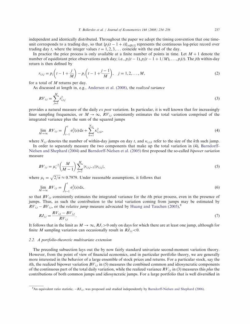
Before presenting the results for all of the 40 stocks and the EQW index, it is instructive to look at thedifferent variation measures and the BN–S test for a single stock and a few specific days in the sample. To thisend, Fig. 2 shows the price (adjusted for stock splits) and returns for PG. While the price appears to be steadily

ARTICLE IN PRESS

11The criteria used in selecting the 40 stocks are discussed in more detail in the Data Appendix. The specific ticker symbols for each of

the stocks are included in many of the figures.12For simplicity we decided to maintain the identical sampling frequency across all stocks. However, M ¼ 22 is clearly a conservative

choice for many of the stocks, and we also calculated the same statistics based on finer sampled high-frequency returns. Subsampling

techniques could also be used to further enhance the accuracy of the realized variation measures and test statistics. The results from some

of these additional calculations are briefly discussed below.13At the 5-min interval the correlation is 0.88.


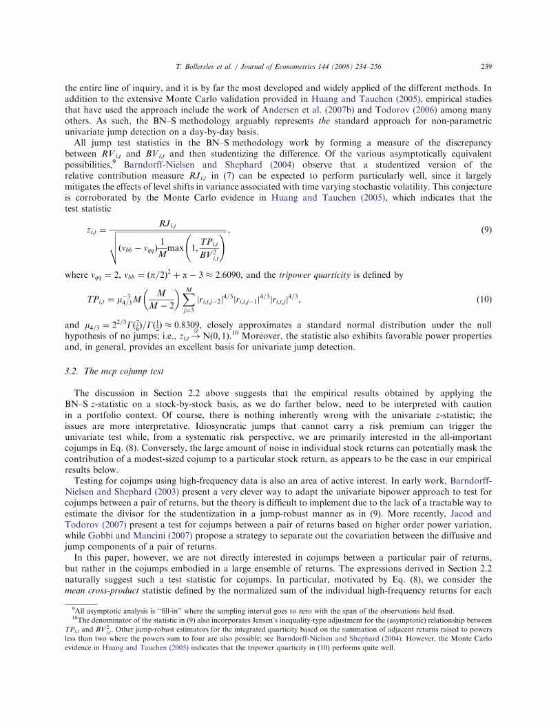
increasing over the 1,241 trading days in the 2001–2005 sample, the corresponding 27,302 high-frequency17.5min returns are all seemingly scattered around zero. At the same time, the return plot clearly indicates thepresence of volatility clustering. This is further underscored by Fig. 3, which plots the RVt and BVt variation

ARTICLE IN PRESS

2001 2002 2003 2004 200560708090

100110

Year

Year

Pric

e, $

2001 2002 2003 2004 2005−6−4−2

0246

Ret

ums,

%

Fig. 2. Prices and returns for PG from 2001 to 2005, M ¼ 22.

2001 2002 2003 2004 2005

5

10

15

Realized Variance

Year

2001 2002 2003 2004 2005

5101520

Bipower Variation

Year

2001 2002 2003 2004 2005−40−20

0204060

Relative Jump

Year

2001 2002 2003 2004 2005

−2

0

2

4z

Year

Φ−1(0�999)

Fig. 3. Return, realized variance, bipower variation, relative jump, and zt-statistic for PG from 2001 to 2005, M ¼ 22.


measures, the relative jump contribution RJt, along with the BN–S z-statistic in Eq. (9). Comparing the BN–Stest statistic in the lower plot to the horizontal reference line for the 99.9% significance level included in theplot, indicates that PG jumped at least once during the active part of the trading day on 17 days in the sample.

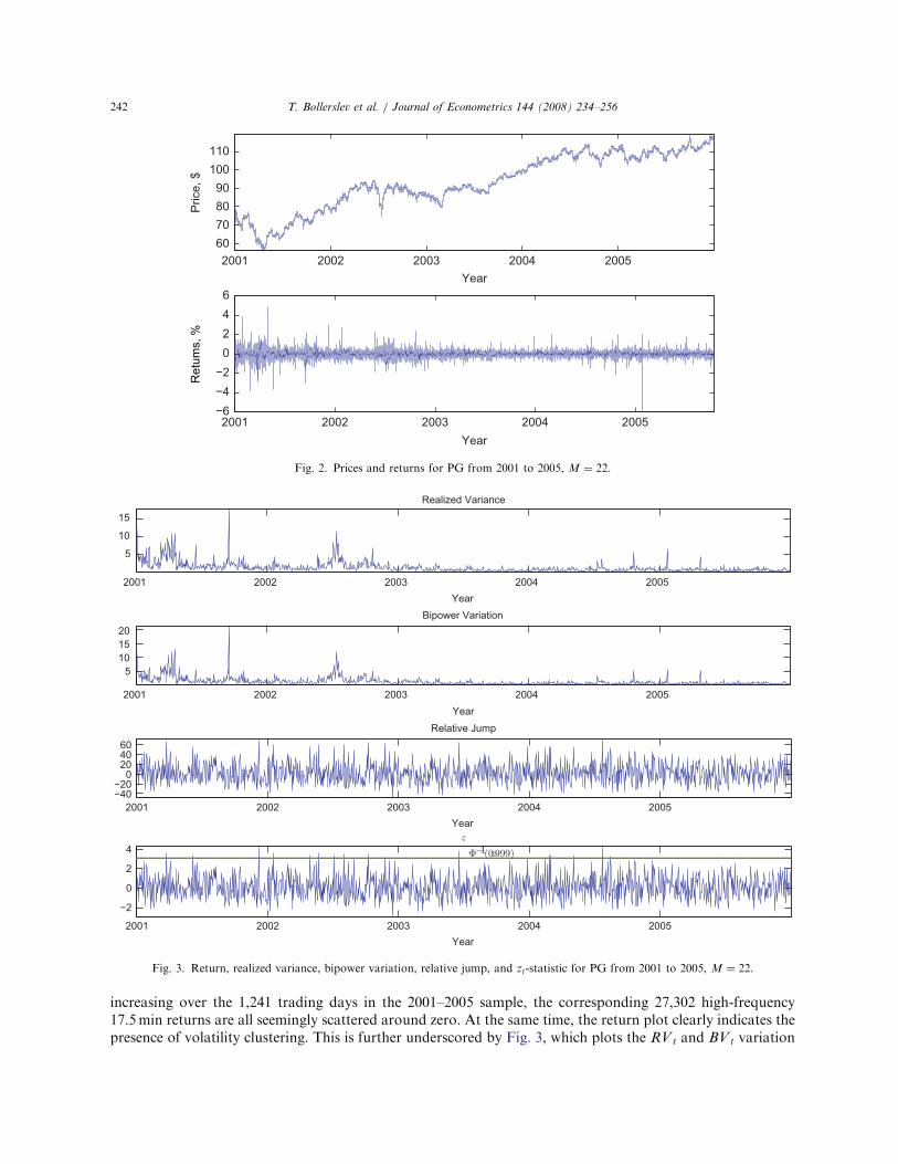
To further illustrate the working of the jump detection scheme, Fig. 4 shows the intraday prices and returnsfor PG on March 26 and 27, 2001. At a first glance it appears as if the price evolves rather smoothly on the26th, while it shows a rather sharp increase just before noon on the 27th. Nonetheless, the correspondingBN–S z-statistics equal to 3.63 and �0:20 for each of the two days, respectively, suggest at least one highlysignificant jump on the 26th and no jumps on the 27th. Importantly, the jump test statistic depends on boththe magnitude of the largest price change(s) over the day and the overall level of the volatility for the day. Assuch, relatively small price changes may be classified as jumps on otherwise calm days, while apparentdiscontinuities may be entirely compatible with a continuous sample path process in a statistical sense on veryvolatility days. Indeed, looking at the plot of the returns in the lower panel, the overall level of the volatilitywas clearly much higher on the 27th than on the 26th, with the BVt estimate for the continuous sample pathvariation for each of the two days equal to 5.11 and 1.04, respectively. Thus, while some of the statisticallysignificant jumps identified by the BN–S test can rather easily be spotted by ex post visual inspection of theintraday prices that is not necessarily always the case.

5. Jumps and cojumps

5.1. Univariate analysis

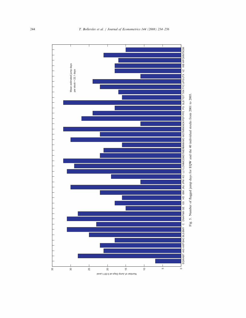
We start with a univariate analysis using the standard BN–S approach applied to the index and each of theindividual stocks on a stock-by-stock basis. Fig. 5 shows the number days over the 2001–2005 sample periodon which the BN–S z-statistics indicate that the EQW index and each of the 40 stocks comprising the indexjumped. A day is classified as containing at least one jump if the z-statistic exceeds the critical value of theGaussian distribution at the 0.001 significance level. From the figure, the index is seen to jump on far fewer

ARTICLE IN PRESS

10am 11am 12pm 1pm 2pm 3pm 4pm 10am 11am 12pm 1pm 2pm 3pm 4pm59

59.560

60.561

61.562

62.563

j

Pric

e, $

10am 11am 12pm 1pm 2pm 3pm 4pm 10am 11am 12pm 1pm 2pm 3pm 4pm−1.5

−1

−0.5

0

0.5

1

1.5

j

Ret

urns

, %

Fig. 4. Prices and returns for PG on March 26–27, 2001, M ¼ 22.


ARTICLE IN PRESS

EQ

WA

BT

AIG

AX

PB

AC

BLS

BM

YC

DN

AFN

MG

EG

SH

DIB

MJN

JJP

MK

OLL

YLO

WM

CD

MD

TME

RMM

MM

OM

OTM

RK

NO

KP

EP

PFE

PG

SLB

TGT

TXN

TYC

UP

SU

TXV

ZW

BW

FCW

MTX

OM

05101520253035

Number of Jump Days at 0.001 Level

Mea

n es

timat

ed ju

mp

days

per s

tock

= 2

2.1

days

Fig.5.Number

offlagged

jumpdaysforEQW

andthe40individualstocksfrom

2001to

2005.


days than its components; the count for EQW is seven days while there are 22 jump days on average for theindividual stocks. This finding is a simple consequence of diversification as discussed in Section 2.2.

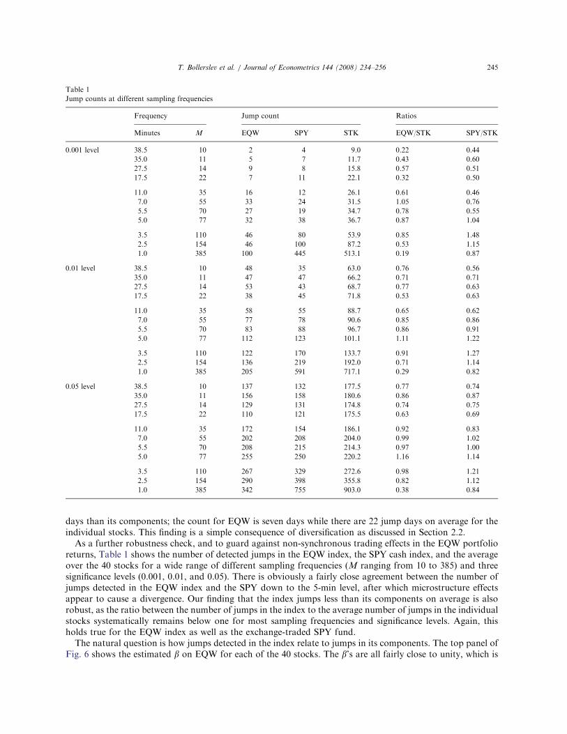
As a further robustness check, and to guard against non-synchronous trading effects in the EQW portfolioreturns, Table 1 shows the number of detected jumps in the EQW index, the SPY cash index, and the averageover the 40 stocks for a wide range of different sampling frequencies (M ranging from 10 to 385) and threesignificance levels (0.001, 0.01, and 0.05). There is obviously a fairly close agreement between the number ofjumps detected in the EQW index and the SPY down to the 5-min level, after which microstructure effectsappear to cause a divergence. Our finding that the index jumps less than its components on average is alsorobust, as the ratio between the number of jumps in the index to the average number of jumps in the individualstocks systematically remains below one for most sampling frequencies and significance levels. Again, thisholds true for the EQW index as well as the exchange-traded SPY fund.

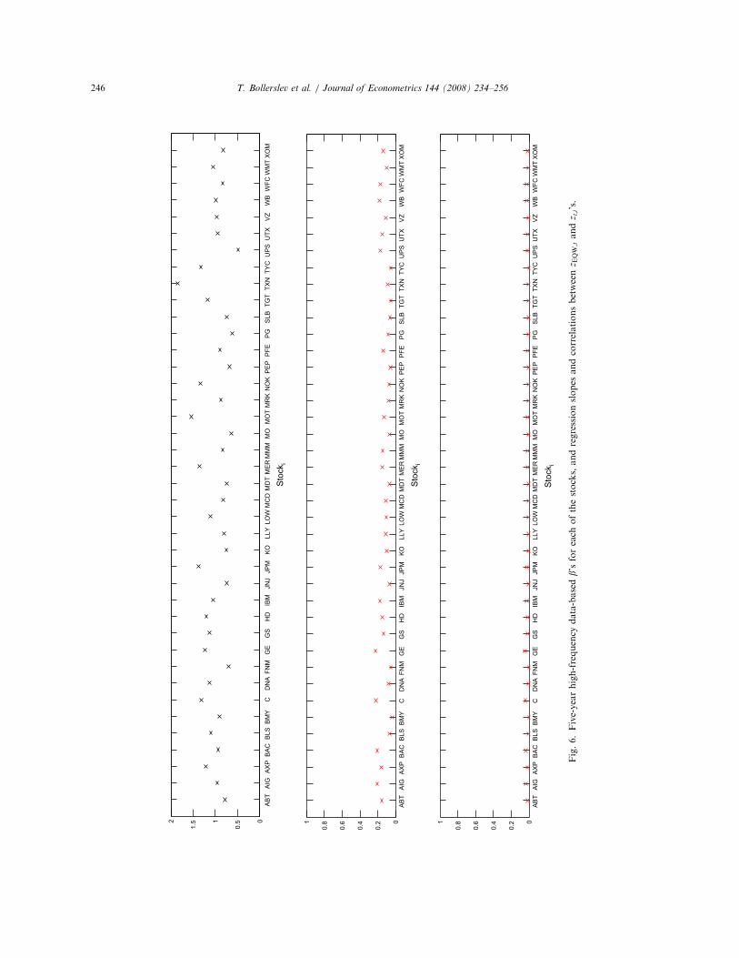
The natural question is how jumps detected in the index relate to jumps in its components. The top panel ofFig. 6 shows the estimated b on EQW for each of the 40 stocks. The b’s are all fairly close to unity, which is

ARTICLE IN PRESS

Table 1

Jump counts at different sampling frequencies

Frequency Jump count Ratios

Minutes M EQW SPY STK EQW/STK SPY/STK

0.001 level 38.5 10 2 4 9.0 0.22 0.44

35.0 11 5 7 11.7 0.43 0.60

27.5 14 9 8 15.8 0.57 0.51

17.5 22 7 11 22.1 0.32 0.50

11.0 35 16 12 26.1 0.61 0.46

7.0 55 33 24 31.5 1.05 0.76

5.5 70 27 19 34.7 0.78 0.55

5.0 77 32 38 36.7 0.87 1.04

3.5 110 46 80 53.9 0.85 1.48

2.5 154 46 100 87.2 0.53 1.15

1.0 385 100 445 513.1 0.19 0.87

0.01 level 38.5 10 48 35 63.0 0.76 0.56

35.0 11 47 47 66.2 0.71 0.71

27.5 14 53 43 68.7 0.77 0.63

17.5 22 38 45 71.8 0.53 0.63

11.0 35 58 55 88.7 0.65 0.62

7.0 55 77 78 90.6 0.85 0.86

5.5 70 83 88 96.7 0.86 0.91

5.0 77 112 123 101.1 1.11 1.22

3.5 110 122 170 133.7 0.91 1.27

2.5 154 136 219 192.0 0.71 1.14

1.0 385 205 591 717.1 0.29 0.82

0.05 level 38.5 10 137 132 177.5 0.77 0.74

35.0 11 156 158 180.6 0.86 0.87

27.5 14 129 131 174.8 0.74 0.75

17.5 22 110 121 175.5 0.63 0.69

11.0 35 172 154 186.1 0.92 0.83

7.0 55 202 208 204.0 0.99 1.02

5.5 70 208 215 214.3 0.97 1.00

5.0 77 255 250 220.2 1.16 1.14

3.5 110 267 329 272.6 0.98 1.21

2.5 154 290 398 355.8 0.82 1.12

1.0 385 342 755 903.0 0.38 0.84


ARTICLE IN PRESS

AB

TA

IGA

XP

BA

CB

LSB

MY

CD

NA

FNM

GE

GS

HD

IBM

JNJ

JPM

KO

LLY

LOW

MC

DM

DT

ME

RM

MM

MO

MO

TM

RK

NO

KP

EP

PFE

PG

SLB

TGT

TXN

TYC

UP

SU

TXV

ZW

BW

FCW

MT

XO

M0

0.51

1.52

Sto

cki

AB

TA

IGA

XP

BA

CB

LSB

MY

CD

NA

FNM

GE

GS

HD

IBM

JNJ

JPM

KO

LLY

LOW

MC

DM

DT

ME

RM

MM

MO

MO

TM

RK

NO

KP

EP

PFE

PG

SLB

TGT

TXN

TYC

UP

SU

TXV

ZW

BW

FCW

MT

XO

M0

0.2

0.4

0.6

0.81

Sto

cki

AB

TA

IGA

XP

BA

CB

LSB

MY

CD

NA

FNM

GE

GS

HD

IBM

JNJ

JPM

KO

LLY

LOW

MC

DM

DT

ME

RM

MM

MO

MO

TM

RK

NO

KP

EP

PFE

PG

SLB

TGT

TXN

TYC

UP

SU

TXV

ZW

BW

FCW

MT

XO

M0

0.2

0.4

0.6

0.81

Sto

cki

Fig.6.Five-yearhigh-frequency

data-basedb’sforeach

ofthestocks,andregressionslopes

andcorrelationsbetweenz E

QW;tandz t;i’s.


not surprising for large-cap stocks. The b’s suggest that the returns on each stock moves approximately one-for-one with the index return, apart from the idiosyncratic component. In particular, large movements, orjumps, in the index should show up as large movements or jumps in the stock prices. On the basis of theestimated b’s, one might expect a reasonably high correlation between a measure of the likelihood of a jump inthe index and a jump in the individual stock prices. The BN–S z-statistic (9) is such a measure. The middlepanel of Fig. 6 shows the 40 regression slope coefficients while the bottom panel shows the 40 estimatedcorrelations between the stock z-statistics and the EQW z-statistic. Interestingly, the correlations areexceedingly low: rarely above 0.05 and frequently lower than 0.01, while the regression slope coefficients aresimilarly small and insignificant.

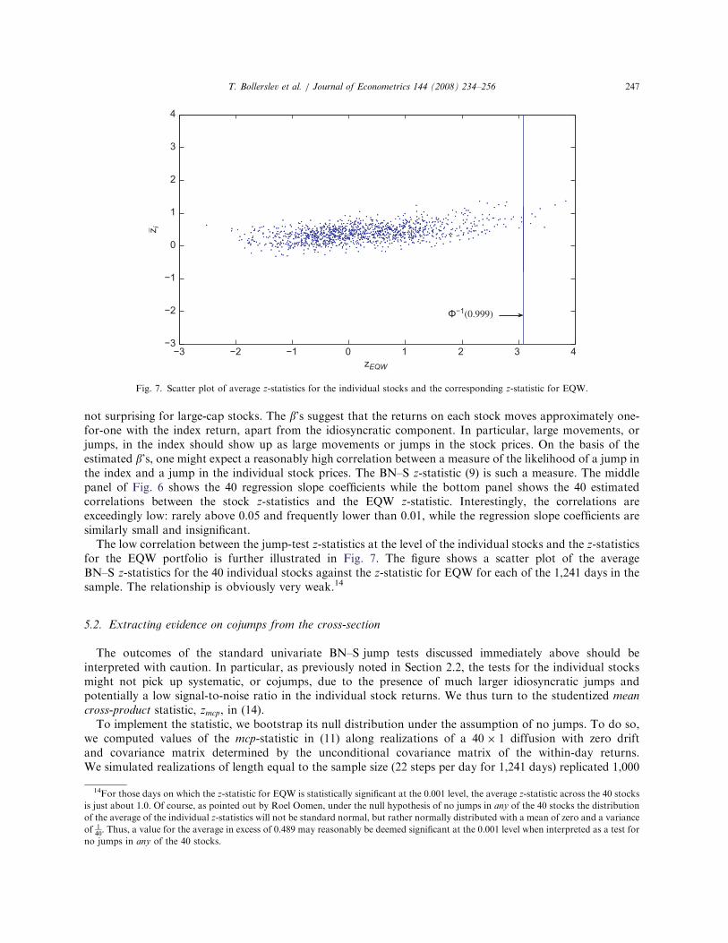
The low correlation between the jump-test z-statistics at the level of the individual stocks and the z-statisticsfor the EQW portfolio is further illustrated in Fig. 7. The figure shows a scatter plot of the averageBN–S z-statistics for the 40 individual stocks against the z-statistic for EQW for each of the 1,241 days in thesample. The relationship is obviously very weak.14

5.2. Extracting evidence on cojumps from the cross-section

The outcomes of the standard univariate BN–S jump tests discussed immediately above should beinterpreted with caution. In particular, as previously noted in Section 2.2, the tests for the individual stocksmight not pick up systematic, or cojumps, due to the presence of much larger idiosyncratic jumps andpotentially a low signal-to-noise ratio in the individual stock returns. We thus turn to the studentized mean

cross-product statistic, zmcp, in (14).To implement the statistic, we bootstrap its null distribution under the assumption of no jumps. To do so,

we computed values of the mcp-statistic in (11) along realizations of a 40� 1 diffusion with zero driftand covariance matrix determined by the unconditional covariance matrix of the within-day returns.We simulated realizations of length equal to the sample size (22 steps per day for 1,241 days) replicated 1,000

ARTICLE IN PRESS

−3 −2 −1 0 1 2 3 4−3

−2

−1

0

1

2

3

4

zEQW

z i

Φ−1(0.999)

Fig. 7. Scatter plot of average z-statistics for the individual stocks and the corresponding z-statistic for EQW.

14For those days on which the z-statistic for EQW is statistically significant at the 0:001 level, the average z-statistic across the 40 stocks

is just about 1.0. Of course, as pointed out by Roel Oomen, under the null hypothesis of no jumps in any of the 40 stocks the distribution

of the average of the individual z-statistics will not be standard normal, but rather normally distributed with a mean of zero and a variance

of 140. Thus, a value for the average in excess of 0.489 may reasonably be deemed significant at the 0.001 level when interpreted as a test for

no jumps in any of the 40 stocks.


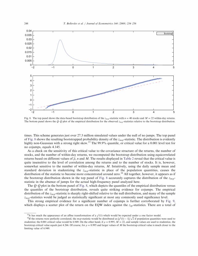
times. This scheme generates just over 27.3 million simulated values under the null of no jumps. The top panelof Fig. 8 shows the resulting bootstrapped probability density of the zmcp-statistic. The distribution is evidentlyhighly non-Gaussian with a strong right skew.15 The 99.9% quantile, or critical value for a 0.001 level test forno cojumps, equals 4.145.

As a check on the sensitivity of this critical value to the covariance structure of the returns, the number ofstocks, and the number of within-day returns, we recomputed the bootstrap distribution using equicorrelatedreturns based on different values of r, n and M. The results displayed in Table 2 reveal that the critical value isquite insensitive to the level of correlation among the returns and to the number of stocks. It is, however,somewhat sensitive to the number of within-day returns, M. Intuitively, using the daily sample mean andstandard deviation in studentizing the zmcp-statistic in place of the population quantities, causes thedistribution of the statistic to become more concentrated around zero.16 All together, however, it appears as ifthe bootstrap distribution shown in the top panel of Fig. 8 accurately captures the distribution of the zmcp-statistic in the absence of jumps for the actual high-frequency panel analyzed here.

The Q–Q plot in the bottom panel of Fig. 8, which depicts the quantiles of the empirical distribution versusthe quantiles of the bootstrap distribution, reveals quite striking evidence for cojumps. The empiricaldistribution of the zmcp-statistic is sharply right-shifted relative to the null distribution, and many of the samplezmcp-statistics would be judged as statistically significant at most any commonly used significance level.

This strong empirical evidence for a significant number of cojumps is further corroborated by Fig. 9,which displays a scatter plot of the return on the EQW index against the zcp-statistics. There are a total of

ARTICLE IN PRESS

−2 −1 0 1 2 3 4 50

0.0050.01

0.0150.02

0.0250.03

0.0350.04

Bootstrap

−2 −1 0 1 2 3 4 5−2

−1

0

1

2

3

4

5

Fig. 8. The top panel shows the data-based bootstrap distribution of the zmcp-statistic with n ¼ 40 stocks and M ¼ 22 within-day returns.

The bottom panel shows the Q–Q plot of the empirical distribution for the observed zmcp-statistics relative to the bootstrap distribution.

15It has much the appearance of an affine transformation of a w2ð1Þ which would be expected under a one factor model.16If the returns were perfectly correlated, the mcp-statistic would be distributed as ½w2ð1Þ � 1�=

ffiffiffi2

pif population quantities were used to

studentize; the 0:001 critical value would be 6:949. On the other hand, if r ¼ 0:995, M ¼ 22, and sample values are used to studentize, the

bootstrap critical value equals just 4.266. Of course, for r ¼ 0:995 and larger values of M the bootstrap critical value is much closer to the

limiting value of 6.949.


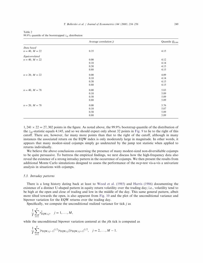
1; 241� 22 ¼ 27; 302 points in the figure. As noted above, the 99.9% bootstrap quantile of the distribution ofthe zcp-statistic equals 4.145, and so we should expect only about 32 points in Fig. 9 to lie to the right of thiscutoff. There are, however, far many more points than that to the right of the cutoff, although in manyinstances the associated return on the EQW index is only moderately large in magnitude. In other words, itappears that many modest-sized cojumps simply go undetected by the jump test statistic when applied toreturns individually.

We believe the above conclusions concerning the presence of many modest-sized non-diversifiable cojumpsto be quite persuasive. To buttress the empirical findings, we next discuss how the high-frequency data alsoreveal the existence of a strong intraday pattern in the occurrence of cojumps. We then present the results fromadditional Monte Carlo simulations designed to assess the performance of the mcp-test vis-a-vis a univariateanalysis in situations with cojumps.

5.3. Intraday patterns

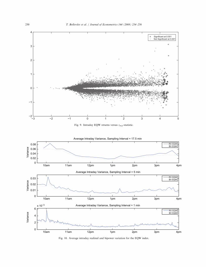
There is a long history dating back at least to Wood et al. (1985) and Harris (1986) documenting theexistence of a distinct U-shaped pattern in equity return volatility over the trading day; i.e., volatility tend tobe high at the open and close of trading and low in the middle of the day. This same general pattern, albeitmore tilted towards the open, is also apparent from Fig. 10 and the plot of the unconditional variance andbipower variation for the EQW returns over the trading day.

Specifically, we compute the unconditional realized variance for tick j as

1

T

XTt¼1

r2EQW;t;j ; j ¼ 1; . . . ;M,

while the unconditional bipower variation centered at the jth tick is computed as

1

T

XTt¼1

jrEQW;t;j�1j1=2jrEQW;t;jjjrEQW;t;jþ1j1=2; j ¼ 2; . . . ;M � 1.

ARTICLE IN PRESS

Table 2

99.9% quantile of the bootstrapped zcp distribution

Average correlation r Quantile Q0:999

Data based

n ¼ 40, M ¼ 22 0.35 4.15

Equicorrelated

n ¼ 40, M ¼ 22 0.00 4.12

0.10 4.14

0.50 4.15

0.80 4.15

n ¼ 20, M ¼ 22 0.00 4.09

0.10 4.14

0.50 4.15

0.80 4.15

n ¼ 40, M ¼ 78 0.00 5.83

0.10 5.89

0.50 5.89

0.80 5.89

n ¼ 20, M ¼ 78 0.00 5.76

0.10 5.87

0.50 5.89

0.80 5.89


ARTICLE IN PRESS


0.02

0.04

0.06

0.08

Var

ianc

e

Average Intraday Variance, Sampling Interval = 17.5 min

RV EQWBV EQW


0.01

0.02

0.03

Var

ianc

e

Average Intraday Variance, Sampling Interval = 5 min

RV EQWBV EQW


2

4

6x 10−3

Var

ianc

e


RV EQWBV EQW

Fig. 10. Average intraday realized and bipower variation for the EQW index.

−3 −2 −1 0 1 2 3 4 5−2

−1

0

1

2

3

4Significant at 0.001Not Significant at 0.001

Fig. 9. Intraday EQW returns versus zmcp-statistic.


Fig. 10 shows these unconditional variance measures at three increasingly finer sampling frequencies:M ¼ 22; 77, and 385, corresponding to 17.5, 5, and 1min, respectively.17 The unconditional realized variancesystematically lies above the unconditional bipower variation over the entire day, thus reflecting the existenceof jumps across the day. Interestingly, however, the plot also reveals a sharp rise in the realized variationrelative to the bipower variation at 10 am EST, corresponding to the time of the release of several regularlyscheduled macroeconomic news announcements.18 This therefore indirectly suggests that some of the cojumpsmay be associated with these types of systematic news. This is also consistent with the work of Andersen et al.(2003, 2007a) among others, which document a significant response in high-frequency financial market pricesto surprises in macroeconomic announcement immediately after the release of the news. Moreover, Andersenand Bollerslev (1998) among others have previously noted a sharp increase in the average total intradayvolatility at the exact time of important macroeconomic news announcements. What is particularlynoteworthy is the much less dramatic increase in the average within-day bipower variation measure, in turnattributing most of the variation at that specific time-of-day to jumps.

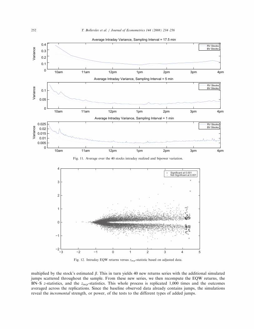
Instead of averaging all of the individual returns before calculating the intraday variation measures as inFig. 10, Fig. 11 shows a similar plot in which the two variation measures are first computed on a stock-by-stock basis and then averaged across all of the 40 stocks in the panel. This explicitly excludes the effect ofdiversification, and as a result the vertical scale of Fig. 11 is much larger than that of Fig. 10. Moreimportantly, however, comparing the general shape between the two sets of pictures, the increase in the within-day variation at 10 am is much less apparent for the individual stock averages. The relative importance ofjumps also appears to be much more evenly distributed across the entire day, and as such lend further credenceto our hypothesis of the cojumps drowning in the firm-specific variation inherent in the individual stockreturns.

The zmcp-statistic in (14) that we used in testing for cojumps was based on the assumption of constant scalewithin the day. The average within-day patterns in Fig. 11 clearly seem to violate this assumption. There is noobvious right way to adjust the individual returns for the intraday volatility patterns, as the relativeimportance of the jump variation to the total variation may be changing over the day. Fortunately, that doesnot seem to matter much for our main conclusions. The cojump statistics depicted in Fig. 9 were based on theraw unadjusted returns ignoring the intraday pattern. As a robustness check we redid the same calculations inwhich we scaled the return for the ith stock over the jth time-interval by the reciprocal of the square root of thecorresponding unconditional bipower variation for that particular stock and time-interval. This adjustment isextreme, in that it deflates returns near the beginning and the end of the day while inflating returns in themiddle of the day under the implicit presumption that the share of the jump variance remains constantover the day. Nonetheless, the resulting Fig. 12 depicting the returns on the EQW index against the adjustedzcp-statistics, is so similar to the original Fig. 9 that we conjecture any reasonable adjustment for the intradaypattern would result in the same basic conclusions.

5.4. Power

Our main conclusions hinge on the argument that the zmcp-statistic is more sensitive to modest-sizedcojumps than the BN–S z-statistic applied stock-by-stock because it explicitly utilizes the cross-sectionalinformation. To investigate this hypothesis further, we use another bootstrap-type procedure where we takethe observed data set as given, sprinkle in additional simulated jumps, and then recompute the jump teststatistics. Importantly, this circumvents the need to specify a complete data generating process for the full40-dimensional vector return process, as would be required by a more traditional simulation-based procedure.

Specifically, for idiosyncratic jumps we simulated 40 independent Gaussian compound Poisson processeswith intensity li and magnitude Nð0;s2J ;iÞ, while for the common jumps we simulated one Gaussian compoundPoisson process with intensity l and magnitude Nð0;s2JÞ. The idiosyncratic jumps are then added to theactually observed within-day 17.5min returns for each of the individual stocks as are the common jumps

ARTICLE IN PRESS

17For visual comparisons, we extended the bipower variation directly to the left for j ¼ 1 and to the right for j ¼ M.18There is also a smaller less pronounced peak at 1:15 pm. However, other computations by Peter Van Tassel, not shown here, suggest

that this early afternoon peak is more fragile. Also, the pattern in Fig. 10 for the EQW portfolio essentially mirrors that for the SPY.


multiplied by the stock’s estimated b. This in turn yields 40 new returns series with the additional simulatedjumps scattered throughout the sample. From these new series, we then recompute the EQW returns, theBN–S z-statistics, and the zmcp-statistics. This whole process is replicated 1,000 times and the outcomesaveraged across the replications. Since the baseline observed data already contains jumps, the simulationsreveal the incremental strength, or power, of the tests to the different types of added jumps.

ARTICLE IN PRESS

−3 −2 −1 0 1 2 3 4 5−2

−1

0

1

2

3

4Significant at 0.001Not Significant at 0.001

Fig. 12. Intraday EQW returns versus zmcp-statistic based on adjusted data.


0.1

0.2

0.3

0.4

Var

ianc

e

Average Intraday Variance, Sampling Interval = 17.5 min

RV StocksBV Stocks


0.05

0.1

Var

ianc

e


RV StocksBV Stocks


0.0050.01

0.0150.02

0.025

Var

ianc

e


RV StocksBV Stocks

Fig. 11. Average over the 40 stocks intraday realized and bipower variation.


The findings for different jump sizes holding the intensities constant are readily described and intuitivelyplausible. In the absence of any common jumps, as the idiosyncratic jump sizes increase from 0% to 1.50%,the jump detection rate of the BN–S z-statistic applied to the individual stocks gradually increases. However, itremains unchanged when applied to the EQW return, as does the detection rate of the zmcp-statistic. Theidiosyncratic jumps are effectively diversified away. On the other hand, if the idiosyncratic jumps are left outwhile the size of the common jump increases from 0% to 1.50%, the detection rates of both the BN–Sz-statistics and zmcp-statistics increase, with the zmcp-statistic being slightly more sensitive to larger jump sizes.Still, the contrasts between the two tests appear rather small, as they both fairly easily detect the occasionalrare common jump.

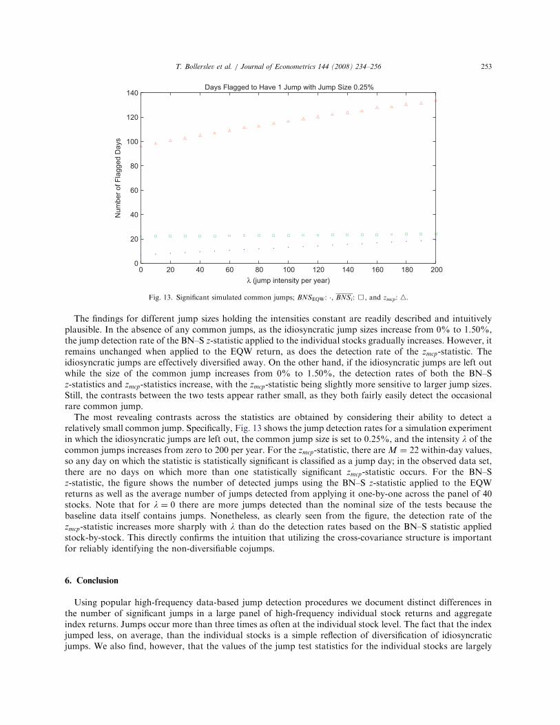
The most revealing contrasts across the statistics are obtained by considering their ability to detect arelatively small common jump. Specifically, Fig. 13 shows the jump detection rates for a simulation experimentin which the idiosyncratic jumps are left out, the common jump size is set to 0.25%, and the intensity l of thecommon jumps increases from zero to 200 per year. For the zmcp-statistic, there are M ¼ 22 within-day values,so any day on which the statistic is statistically significant is classified as a jump day; in the observed data set,there are no days on which more than one statistically significant zmcp-statistic occurs. For the BN–Sz-statistic, the figure shows the number of detected jumps using the BN–S z-statistic applied to the EQWreturns as well as the average number of jumps detected from applying it one-by-one across the panel of 40stocks. Note that for l ¼ 0 there are more jumps detected than the nominal size of the tests because thebaseline data itself contains jumps. Nonetheless, as clearly seen from the figure, the detection rate of thezmcp-statistic increases more sharply with l than do the detection rates based on the BN–S statistic appliedstock-by-stock. This directly confirms the intuition that utilizing the cross-covariance structure is importantfor reliably identifying the non-diversifiable cojumps.

6. Conclusion

Using popular high-frequency data-based jump detection procedures we document distinct differences inthe number of significant jumps in a large panel of high-frequency individual stock returns and aggregateindex returns. Jumps occur more than three times as often at the individual stock level. The fact that the indexjumped less, on average, than the individual stocks is a simple reflection of diversification of idiosyncraticjumps. We also find, however, that the values of the jump test statistics for the individual stocks are largely

ARTICLE IN PRESS

0 20 40 60 80 100 120 140 160 180 2000

20

40

60

80

100

120

140

λ (jump intensity per year)

Days Flagged to Have 1 Jump with Jump Size 0.25%

Num

ber o

f Fla

gged

Day

s

Fig. 13. Significant simulated common jumps; BNSEQW: �, BNSi: &, and zmcp: n.


uncorrelated with the values of the test statistic for an index constructed from the very same stocks. This lackof correlation is interesting in view of the fact that all of the stocks have a b of about unity with respect to theindex. Apparently, the high level of idiosyncratic noise in the individual stock returns masks many of thecojumps that cause the index to jump. To more effectively detect cojumps, we develop a new cross-product

statistic, termed the mcp-statistic, that is motivated by portfolio theory and directly uses the cross-covariationstructure of the high-frequency returns. Employing this statistic we successfully detect many modest-sizedcojumps embodied in the panel of returns.

We also find new evidence for an important intraday pattern in the arrival of cojumps. The stocks in ourpanel show a strong tendency to move sharply together, i.e., cojump, around 10 am Eastern time,corresponding to the regularly scheduled release-time for many macroeconomic news announcements. Thisnewly documented within-day shift in the relative importance of cojumps is overlaid on top of the usualdistinct U-shaped pattern in equity return volatility over the trading day along with the secular longer-runday-to-day movements in the overall level of the volatility.

Documenting the presence of cojumps and understanding their economic determinants and dynamics arecrucial from a risk measurement and management perspective. Basic portfolio theory implies that the onlykind of jumps that can carry a risk premium are a non-diversifiable cojumps. Measuring the risk premium oncojumps is far beyond the scope of the present paper. However, using index-level data Todorov (2006) makesprogress towards separating the aggregate jump risk premium from the continuous volatility risk premiumand understanding its dynamics. The ideas and techniques developed here may prove especially useful infuture work along these lines.

Acknowledgments

The work of Bollerslev was supported by a grant from the NSF to the NBER and CREATES funded by theDanish National Research Foundation. We would like to thank the editor, two anonymous referees, and RoelOomen for their comments, which helped to improve the exposition and sharpen the focus of the paper. Wewould also like to thank members of the Duke University Econometrics and Finance Lunch Group andparticipants at the April 21–22, 2007 Stevanovich conference on ‘‘Volatility and High Frequency Data’’ andthe May 18–19, 2007, ‘‘Financial Econometrics Conference’’ at Imperial College, London, for usefulsuggestions and comments. We are especially grateful to Viktor Todorov and Xin Huang for many discussionsand encouragement along the way.

Appendix A. Data appendix

We initially selected the 50 most actively traded stocks on the New York Stock Exchange (NYSE) accordingto their 10-day trading volume (number of shares) at the beginning of June 2006. Of these 50 stocks, we wereable to successfully download reliable high-frequency prices for 40. The ticker symbols for these 40 stocks areincluded in many of the figures.

A.1. Data source and cleaning

Data on all completed trades were obtained from the Trade and Quote Database (TAQ) available via theWharton Research Data Services (WRDS). This includes trades from all North American exchanges as well asover-the-counter trades. Each exchange has its own distinct market structure which might affect the structureof observed prices. Hence, to homogenize the data, we decided to only consider trades on the NYSE. TheNYSE also accounts for the majority of the trades for all of the stocks in the sample.

Our sample covers the period from January 1st 2001 to December 31st 2005. Trading frequency increasedsignificantly in the late 1990s, and by the end of 2001 all NYSE listed stocks had moved from fractional todecimalized trading, in turn allowing for the extraction of highly reliable high-frequency prices. Illogical datavalues such as time stamp errors (e.g., hour #25, minute #78, month #43 and year #3001) and negative pricesare removed from the data. All-in-all, these errors represent a relatively small number of data points. We alsoexclude trades that occur outside of 9.30 am and 4 pm, as well as days with only partial trading. Examples of


such days are September 11, 2001, and certain holidays when the NYSE is only open for part of the day.A listing of all of these dates is available on the NYSE web-site.

Because of the unusual activity associated with trading at the beginning of each day, we start our intradaysampling at 9.35 am, 5-min after the market officially opens. This ensures a more homogenous trading andinformation gathering mechanism for all of the prices. The price series are sampled every 30-s using a slightlymodified version of the previous tick method from Dacorogna et al. (2001). The previous tick method simplyfixes the time where prices are ideally sampled at regular intervals and selects a completed trade prior to thetime should there be no trade at that particular time. For instance, a trade completed at 9:34:58 is used in placeof 9:35:00 when there is no actual trade at 9:35:00. In this case, there is therefore a 2-s backtrack, as defined bythe time difference between the ideal sampling time and the actual sampling time. The first trade of the day isused if there are no prior trades on that day. With 30-s sampling from 9.35 am to 4.00 pm this leaves us with771 prices per day. Also, the sample period from January 1st 2001 through December 31st 2005 consists of1,241 normal trading days, for a total of close to a million transaction prices for each of the 40 individualstocks.

The raw high-frequency prices invariable contains a number of mis-recordings and other data errors. Insome cases these errors are obvious by visual inspection of time series plots of the data, sometimes they arenot. Thus, in addition to manually inspecting and correcting the data, we also employed a threshold filter of1.5%, which appears to work well for removing and cleaning the remaining data errors at the 30-s samplinginterval.

A.2. Sampling frequency

The statistics used in the paper formally becomes more accurate as the sampling frequency increases.However, as noted in the main text of the paper, there is a limit to how finely we can sample the price processwhile maintaining the basic underlying semimartingale assumption as a host of market microstructureinfluences start to materially affect the observed price changes; most importantly features having to do withspecifics of the trading mechanism, Black (1976) and Amihud and Mendelson (1987), and discreteness of thedata (Harris, 1990, 1991). As discussed at length in Hansen and Lunde (2006), the design of new proceduresand ‘‘optimal’’ ways in which to deal with these complications is currently the focus of extensive researchefforts. Rather than employing any of these more advanced procedures, in the analysis reported on here, wesimply rely on the volatility signature plots proposed by Andersen et al. (2000) as an easy-to-implementprocedure for choosing the highest possible sampling frequency so that the realized variation measures remainunbiased for the unconditional daily variance.

The corresponding plots for each of the 40 stocks (available upon request) suggest that by sampling M ¼ 22times per day, or equivalently by using 17.5min returns, the market microstructure influences have essentiallyceased and the plots for the realized variation measures become flat. Of course, for many of the stocks wecould safely sample more frequently, but for simplicity we decided to maintain the identical samplingfrequency across all 40 stocks throughout the entire sample. Importantly, the choice of M ¼ 22 also involvesrelatively little interpolation in the construction of the equidistant 17.5min returns. The median backtrackfrom the previous tick method for each of the 40 stocks is just about 6.5 s, and for none of the stocks does themedian backtrack exceed 12 s.

References

Ait-Sahalia, Y., Jacod, J., 2008. Testing for jumps in a discretely observed process. Annals of Statistics, forthcoming.

Ait-Sahalia, Y., Mykland, P., Zhang, L., 2005. How often to sample a continuous time process in the presence of market microstructure

noise. Review of Financial Studies 18, 351–416.

Amihud, Y., Mendelson, H., 1987. Trading mechanisms and stock returns: an empirical investigation. Journal of Finance 42, 533–553.

Andersen, T., Bollerslev, T., 1998. Deutschemark-dollar volatility: intraday activity patterns, macroeconomic announcements, and longer

run dependencies. Journal of Finance 53, 219–265.

Andersen, T., Bollerslev, B., Diebold, F., Labys, P., 2000. Great realizations. Risk 13, 105–108.

Andersen, T., Bollerslev, T., Diebold, F., 2008. Parametric and nonparametric volatility measurement. In: Ait-Sahalia, Y., Hansen, L.P.

(Eds.), Handbook of Financial Econometrics. North-Holland, Amsterdam.

ARTICLE IN PRESST. Bollerslev et al. / Journal of Econometrics 144 (2008) 234–256 255

Andersen, T., Bollerslev, B., Diebold, F., Vega, C., 2003. Micro effects of macro announcements: real-time price discovery in foreign

exchange. American Economic Review 93, 38–62.

Andersen, T., Bollerslev, B., Diebold, F., Vega, C., 2007a. Real-time price discovery in stock, bond and foreign exchange markets. Journal

of International Economics 73, 251–277.

Andersen, T., Bollerslev, T., Diebold, F., 2007b. Roughing it up: including jump components in the measurement, modeling and

forecasting of return volatility. Review of Economics and Statistics 89, 701–720.

Bandi, F., Russell, J., 2008. Microstructure noise, realised volatility, and optimal sampling. Reviews of Economic Studies, forthcoming.

Barndorff-Nielsen, O., Shephard, N., 2003. Measuring the impact of jumps in multivariate price processes using bipower covariation.

Working paper, Nuffield College, Oxford University.

Barndorff-Nielsen, O., Shephard, N., 2004. Power and bipower variation with stochastic volatility and jumps. Journal of Financial

Econometrics 2, 1–37.

Barndorff-Nielsen, O., Shephard, N., 2006. Econometrics of testing for jumps in financial economics using bipower variation. Journal of

Financial Econometrics 4, 1–30.

Barndorff-Nielsen, O., Graversen, S., Jacod, J., Podolskij, M., Shephard, N., 2005. A central limit theorem for realised power and bi-

power variations of continuous semimartingales. Working paper, Nuffield College, Oxford University.

Barndorff-Nielsen, O., Hansen, P., Lunde, A., Shephard, N., 2006. Designing realised kernels to measure the ex post variation of equity

prizes in the presence of noise. Working paper, Nuffield College, Oxford University.

Basawa, I., Brockwell, P., 1982. Non-parametric estimation for non-decreasing Levy processes. Journal of the Royal Statistical Society

Series B 44, 262–269.

Black, F., 1976. Noise. Journal of Finance 41, 529–543.

Borovkova, S., Burton, R., Dehling, H., 2001. Limit theorems for functionals of mixing processes with applications to U-statistics and

dimension estimation. Transactions of the American Mathematical Society 353, 4261–4318.

Dacorogna, M., Gencay, R., Muller, U., Olsen, R., Pictet, O., 2001. An Introduction to High Frequency Finance. Academic Press, San

Diego.

Eraker, B., Johannes, M., Polson, N., 2003. The impact of jumps in volatility and returns. Journal of Finance 58, 1269–1300.

Fan, J., Wang, Y., 2006. Multi-scale jump and volatility analysis for high-frequency financial data. Working paper, Princeton University.

Gobbi, F., Mancini, C., 2007. Identifying the covariation between the diffusion parts and the co-jumps given discrete observations.

Working paper, Dipartimento di Matematica per le Decisioni, Universita degli Studi di Firenze.

Hansen, P., Lunde, A., 2006. Realized variance and market microstructure noise. Journal of Business and Economic Statistics 24, 127–161.

Harris, L., 1986. A transaction data study of weekly and intradaily patterns in stock returns. Journal of Financial Economics 16, 99–117.

Harris, L., 1990. Estimation of stock variance and serial covariance from discrete observations. Journal of Financial and Quantitative

Analysis 25, 291–306.

Harris, L., 1991. Stock price clustering and discreteness. Review of Financial Studies 4, 389–415.

Huang, X., Tauchen, G., 2005. The relative contributions of jumps to total variance. Journal of Financial Econometrics 3, 456–499.

Jacod, J., Todorov, V., 2007. Testing for common arrivals of jumps for discretely observed multidimensional processes. Working paper,

Duke University.

Jiang, G., Oomen, R., 2006. A new test for jumps in asset prices. Working paper, University of Warwick.

Lee, S., Mykland, P., 2008. Jumps in financial markets: a new nonparametric test and jump dynamics. Review of Financial Studies,

forthcoming.

Mancini, C., 2004. Estimation of the characteristics of the jumps of a general Poisson-diffusion model. Scandinavian Actuarial Journal,

42–52.

Todorov, V., 2006. Variance risk premium dynamics. Working paper, Duke University.

Wood, R., McInish, T., Ord, J., 1985. An investigation of transaction data for NYSE stocks. Journal of Finance 25, 723–739.


Risk, jumps, and diversification

Documents