1 Risk and Return Within the Stock Market: What Works Best? Roger G. Ibbotson * and Daniel Y.-J. Kim ** January 14, 2014 Abstract This paper studies return-predictive characteristics of U.S. securities, including beta, volatility, size, value, liquidity, and momentum. Value and low liquidity have the largest impact on returns, while low beta, low volatility, and low liquidity have the best performance when measured on a risk adjusted basis. Contrary to the conventional wisdom on risk and reward, most portfolio sorting metrics exhibit an inverse risk-return relationship, with lower risk portfolios outperforming higher risk portfolios. A broad theme that emerges from the empirical evidence is that popularity underperforms. * Roger G. Ibbotson is a Professor in Practice at Yale School of Management and Chairman & CIO of Zebra Capital Management, LLC. ** Daniel Y.-J. Kim is Research Director at Zebra Capital Management, LLC.

Welcome message from author
This document is posted to help you gain knowledge. Please leave a comment to let me know what you think about it! Share it to your friends and learn new things together.
Transcript

1
Risk and Return Within the Stock Market:
What Works Best?
Roger G. Ibbotson* and Daniel Y.-J. Kim**
January 14, 2014
Abstract
This paper studies return-predictive characteristics of U.S. securities,
including beta, volatility, size, value, liquidity, and momentum. Value and low
liquidity have the largest impact on returns, while low beta, low volatility, and
low liquidity have the best performance when measured on a risk adjusted
basis. Contrary to the conventional wisdom on risk and reward, most portfolio
sorting metrics exhibit an inverse risk-return relationship, with lower risk
portfolios outperforming higher risk portfolios. A broad theme that emerges
from the empirical evidence is that popularity underperforms.
* Roger G. Ibbotson is a Professor in Practice at Yale School of Management and Chairman & CIO of Zebra Capital Management, LLC. ** Daniel Y.-J. Kim is Research Director at Zebra Capital Management, LLC.
2
It is well known that across asset classes, more risky asset classes beat
less risky assets. Over the long run, stocks outperform bonds in the U.S.1 and
worldwide for almost all extended periods. For example, Dimson, Marsh, and
Staunton (2013) examine equity risk premiums starting in 1900, and find that
stocks outperform bonds in all 20 developed countries studied.
Instead of across stock markets, we look within a single market, the U.S.
stock market. We study the risk and return relationships when categorizing
stocks by various characteristics including beta, volatility, size, value, liquidity,
and momentum. We determine which characteristics have the largest impact
on returns and observe whether higher risk always accompanies higher
returns. Relative to the conventional wisdom on risk and reward, many of the
empirical results are surprising; we offer the underperformance of popularity
as a common explanation for several of these unexpected results.
The Data Set
We use the CRSP (market data) and Compustat (accounting data)
datasets on U.S. stocks, as accessed through the WRDS website2. Portfolios
are constructed annually on the final trading day of each calendar year
between 1971 and 2012, using trailing 12-month (“selection year”) data. In
each selection year, the universe is limited to a maximum of 3,000 stocks, but
1 See Ibbotson SBBI 2013 Classic Yearbook, Market Results for Stocks, Bonds, Bills, and Inflation 1926-2012, Morningstar Inc. Stocks had a compounded annual return of 9.8% over the full period while long-term U.S. Government bonds returned 5.7% and U.S. Treasury Bills returned 3.5%. 2 CRSP (Center for Research in Security Prices) data is from the University of Chicago, Booth School of Business, and Compustat is a trademark of Standard & Poor's, a division of the McGraw-Hill Companies. WRDS (Wharton Research Data Services) is available at wrds-web.wharton.upenn.edu.

3
in about half of the sample period years, the universe consists of fewer than
3,000 stocks, after culling the sample for low capitalizations, low stock prices,
or missing data3. We make use of selection-year data on revenue, earnings,
book equity, and assets when available. Selected portfolios are passively held
in the following calendar year (the “performance year”) to determine the total
returns of portfolios.
In Table 1 we list the equally weighted and capitalization weighted
benchmarks, derived from the universe of stocks in the study. The period
consists of 42 performance years from 1972-2013 (1971 is only used as a
selection year), over which the average number of stocks in the universe
portfolio is 2,602. This period covers several economic cycles, including the
recessions of 1973-74, 1980-81, 1991-92, 2000-2001, and the financial crisis
of 2008. It also includes the strong bull markets of the 1980s and 1990s, so
that the overall returns are still reasonably high and are far in excess of
riskless rates. Thus there is a substantial equity risk premium over the period.
Table 1. Benchmark returns, 1972-2013.
Portfolio Weighting Result
Universe
Equal weight
geom 12.98%
arith 15.22%
SD 22.03%
Cap weight
geom 10.72%
arith 12.27%
SD 17.86% 3 The inclusion criteria for stocks are: common stocks listed on the NYSE, AMEX, or NASDAQ markets, but excluding REITs, warrants, ADRs, ETFs, Americus Trust Components, and closed-end funds. Data for trading volume, total returns, earnings, shares outstanding, and price must be available for the 12 months of the selection year. The stock price at the end of the selection year must be at least $2. Finally, the market capitalization of included companies must both rank within the largest 3,000 for the year, and also exceed a fixed fraction of the total universe market cap at year end, equal to that of a $100 million company at the end of 2011.

4
We will examine the general categories of beta & volatility, size, value,
liquidity, momentum, Fama & French betas, and factor betas of portfolios,
where each of these categories includes various sorting metrics with which the
stock universe is ranked in the selection year by quartiles, with total returns
measured in the following performance year.
In Table 2 as an illustration, we list the median metric values of all
quartile portfolios constructed on the last trading day of selection year 2012.
For example, the row labeled “CAPM beta” lists the median beta of the 4
quartile portfolios constructed by sorting each stock in the universe by beta (as
calculated from daily stock returns during 2012.) Likewise, the row labeled
“Market cap [$B]” shows the median market cap of the 4 size quartiles
constructed using year-end 2012 market cap data.
Accounting data is lagged by 2 months beyond the end of the accounting
reporting period, in order to reflect reporting delays. Thus, in Table 2, the sort
metrics for total assets, revenue, net income, book/market, earnings/price,
and ROE for selection year 2012 are measured using accounting data from
reporting periods ending between November 2011 and October 2012. In
contrast, market cap, market turnover, and momentum are ranked using
calendar year 2012 data.
In Table 2, our naming convention for the quartile portfolios is that the
geometric mean of portfolio Q1 over the 42-year study period always
outperforms that of portfolio Q4.

5
Table 2. Median metric values of all quartile portfolios selected in 2012.
Category Portfolio Sort Metric Q1 Q2 Q3 Q4
Beta & Volatility
CAPM beta 0.714 1.049 1.308 1.738
Daily volatility 0.013 0.018 0.023 0.033
Monthly volatility 0.045 0.071 0.097 0.151
Size
Market Cap [$B] 0.211 0.620 1.792 8.977
Total Assets [$B] 12.712 2.622 0.878 0.224
Revenue [$B] 7.399 1.572 0.506 0.109
Net Income [$B] 0.510 0.085 0.021 -0.023
Value Book/Market 1.099 0.661 0.402 0.175
Earnings/Price 0.099 0.061 0.038 -0.054
ROE 0.236 0.123 0.068 -0.096
Liquidity Amihud [10-6] 0.057 0.007 0.001 0.000
Turnover 0.436 1.041 1.718 3.303
Momentum 12-month 0.577 0.242 0.080 -0.145
2-12 month 0.530 0.204 0.048 -0.173
Fama & French Factor Coefficients
FF Market beta 0.612 0.912 1.155 1.574
FF SMB small size beta -0.046 0.501 0.986 1.604
FF HML high value beta 0.864 0.362 -0.025 -0.529
Single Factor Coefficients
SMB small size beta 0.622 1.207 1.702 2.368
HML high value beta 0.695 0.231 -0.106 -0.606
WML high momentum beta -1.541 -0.997 -0.690 -0.320
LMH low liquidity beta -0.529 -0.877 -1.203 -1.784

6
Comparing the Quartile Portfolios Across Characteristics
Portfolios constructed using selection-year (1971-2012) metrics are
passively held in the subsequent performance year (1972-2013). During the
performance year, no rebalancing takes place, so the position weights are
allowed to float throughout the performance year. The end of each calendar
year thus marks both the end of the performance year for the portfolios
selected one year previously, as well as the construction date for a new set of
selection-year portfolios using recalculated sort metrics listed in Table 2. In
effect, the 84 quartile portfolios listed in Table 2 last for the entire study period
and are rebalanced annually.
We report the annualized geometric mean, the annualized arithmetic
mean, and the annualized monthly standard deviation in the tables that follow.
In Figures 1-8 and Figure 10, we plot the annualized geometric mean
during the study period on the vertical axis and the annualized standard
deviations on the horizontal axis.
Beta and Volatility. We first look at the impact of beta and volatility upon
returns over the period. According to the Sharpe (1964) and Lintner (1965)
capital asset pricing model, there should be a positive relationship between
beta and returns. Even according to more general theories of capital markets,
there should be a positive relationship between risk and return. Thus higher
volatility should also be associated with high returns.

7
In Table 3, we report the long-term performance-year returns for each
quartile portfolio within the Beta & Volatility category of sort metrics. We list
the annualized geometric mean, arithmetic mean, and annualized standard
deviation that were realized during the study period. Again, portfolios Q1
through Q4 are in either strictly increasing or strictly decreasing order in the
portfolio sorting metric, and Q1 denotes whichever extreme in the sorting
metric outperformed over the study time period. For this category of return-
predictive metrics, the Q1 outperforming quartiles are associated with low beta,
low daily volatility, and low monthly volatility from the selection year.
Table 3. Beta & Volatility Quartile portfolio returns, 1972-2013.
Portfolio sort metric Result Q1 Q2 Q3 Q4
CAPM beta Q1 = low
geom 14.42% 14.50% 12.93% 8.80%
arith 15.99% 16.52% 15.41% 12.97%
SD 18.52% 21.16% 23.24% 29.99%
Daily volatility Q1 = low
geom 14.01% 14.53% 13.85% 7.84%
arith 15.27% 16.36% 16.47% 12.79%
SD 16.60% 19.97% 23.86% 33.08%
Monthly volatility Q1 = low
geom 14.41% 14.66% 13.37% 8.00%
arith 15.76% 16.53% 16.05% 12.56%
SD 17.33% 20.23% 24.04% 31.68%
Graphing the quartiles in Figure 1 illustrates these results on an annual
geometric mean vs. annual standard deviation plot. The Q1 quartiles are
shown with pointed up triangles, while the Q4 quartiles are shown with the
pointed down triangles. The middle quartiles Q2 and Q3 are shown with
smaller dots. The risk and return of the equally weighted universe and
capitalization weighted universe portfolios are shown in diamonds. Note that

8
for the Q4 portfolios, high beta, high monthly volatility and high daily volatility
had by far the lowest realized returns, even though they had the most risk.
The Q1 and Q2 portfolios had the highest returns, but with a risk less than the
equally weighted universe portfolio.
Other researchers have previously found that a positive beta and
volatility risk and return relationship do not hold. For example, Black, Jensen,
and Scholes (1972) and Frazzini and Pedersen (2011) find that high beta stocks
are associated with low excess returns, while Haugen and Baker (1991) and
Ang, Hodrick, Xing and Zhang (2006) find that high volatility stocks
consistently underperform.
Figure 1. Beta & Volatility Quartile Portfolios

9
Frazzini and Pedersen (2011) show that leverage aversion on the part of
some market participants results in the popularity of high-volatility, high-beta
securities; this popularity in turn bids up prices and reduces returns.
Size of Companies. The size portfolios are presented in Table 4.
Comparing the quartiles, the small cap premium is positive in that the
geometric mean of small-cap Q1 is 14.08% vs. 11.70% from large-cap Q4, with
small caps having a higher standard deviation.
When we measure company size by total assets, revenue, or net income,
however, it is the larger companies that outperform the smaller companies.
The differences in arithmetic mean return between the Q1 and Q4 portfolios
are not significant, a result that is consistent with previous results (Berk 1997)
that examine accounting-based measures of company size as a predictor of
expected returns.
Table 4. Size Quartile portfolio returns, 1972-2013.
Portfolio sort metric Result Q1 Q2 Q3 Q4
Market Cap Q1 = small cap
geom 14.08% 12.65% 12.92% 11.70%
arith 17.36% 15.18% 15.03% 13.32%
SD 26.98% 23.63% 21.38% 18.33%
Total Assets Q1 = high assets
geom 12.85% 14.36% 13.08% 11.27%
arith 14.63% 16.21% 15.43% 14.78%
SD 19.38% 20.19% 22.58% 27.86%
Revenue Q1 = high revenue
geom 13.79% 13.66% 13.59% 10.68%
arith 15.56% 15.78% 15.98% 13.90%
SD 19.52% 21.39% 22.80% 26.80%
Net Income Q1 = high income
geom 12.83% 13.63% 14.01% 10.76%
arith 14.39% 15.48% 16.48% 14.80%
SD 18.14% 20.12% 23.20% 29.79%

10
Regardless of the metric used, we find that the standard deviation of
returns is much higher for the smaller companies than the larger companies.
As shown in Figure 2, high volatility is associated with small size, however
defined. For small caps, high risk is associated with high returns, while for
small companies, high risk is associated with low returns.
Figure 2. Size Quartiles
11
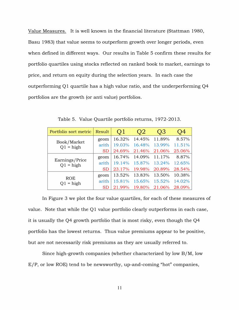
Value Measures. It is well known in the financial literature (Stattman 1980,
Basu 1983) that value seems to outperform growth over longer periods, even
when defined in different ways. Our results in Table 5 confirm these results for
portfolio quartiles using stocks reflected on ranked book to market, earnings to
price, and return on equity during the selection years. In each case the
outperforming Q1 quartile has a high value ratio, and the underperforming Q4
portfolios are the growth (or anti value) portfolios.
Table 5. Value Quartile portfolio returns, 1972-2013.
Portfolio sort metric Result Q1 Q2 Q3 Q4
Book/Market Q1 = high
geom 16.32% 14.45% 11.89% 8.57%
arith 19.03% 16.48% 13.99% 11.51%
SD 24.69% 21.46% 21.06% 25.06%
Earnings/Price Q1 = high
geom 16.74% 14.09% 11.17% 8.87%
arith 19.14% 15.87% 13.24% 12.65%
SD 23.17% 19.98% 20.89% 28.54%
ROE Q1 = high
geom 13.52% 13.83% 13.50% 10.38%
arith 15.81% 15.65% 15.52% 14.02%
SD 21.99% 19.80% 21.06% 28.09%
In Figure 3 we plot the four value quartiles, for each of these measures of
value. Note that while the Q1 value portfolio clearly outperforms in each case,
it is usually the Q4 growth portfolio that is most risky, even though the Q4
portfolio has the lowest returns. Thus value premiums appear to be positive,
but are not necessarily risk premiums as they are usually referred to.
Since high-growth companies (whether characterized by low B/M, low
E/P, or low ROE) tend to be newsworthy, up-and-coming “hot” companies,

12
within the category of value metrics, popularity is again associated with
underperformance in the long term.
Figure 3. Value Quartiles
Liquidity. We measure returns from portfolios formed by ranking two
different measures of liquidity premiums. One measure is the Amihud (2002)
“ILLIQ” metric, defined as the absolute value of the daily return divided by the
daily dollar value of shares traded, averaged over the course of the selection
year. Stocks are ranked during the selection year by this metric, and are
placed into the four quartile portfolios for each performance year. Another
measure of liquidity is the turnover rate (Datar, Naik and Radcliffe 1998), for
which we calculate the monthly ratios of the number of shares traded to the

13
number of shares outstanding, with the twelve monthly turnover rates summed
over the selection year to get the annual turnover rate for each stock. The
stocks are then ranked and placed into the four quartile portfolios.
In Table 6 we show the returns for liquidity according to the two
methods. The low liquidity portfolios are labeled Q1 and the high liquidity
portfolios Q4. For both measures, the low liquidity portfolios outperform by a
wide margin.
Table 6. Liquidity Quartile portfolio returns, 1972-2013.
Portfolio sort metric Result Q1 Q2 Q3 Q4
Amihud Q1 = low liquidity
geom 14.85% 12.31% 12.35% 11.43%
arith 17.74% 14.92% 14.60% 13.17%
SD 25.54% 23.94% 22.11% 18.99%
Turnover Q1 = low liquidity
geom 15.51% 14.42% 12.80% 8.27%
arith 17.33% 16.34% 15.18% 12.05%
SD 20.18% 20.66% 22.74% 28.35%
In Figure 4 we graph the four liquidity quartiles from the Amihud and
turnover measures. Although for both measures the low liquidity Q1 portfolios
outperform, the two measures have completely different risk characteristics.
The low liquidity Amihud measure is the most risky portfolio, whereas the low
turnover portfolios exhibit less risk.
Idiosyncratic liquidity is a multifaceted concept. Since turnover
measures the fraction of a company that changes owners, it encodes popularity
through trading volume, whereas the Amihud metric measures the price
impact of trading and thus is a more “pure” measure of liquidity. Like the

14
categories of beta and volatility previously discussed, here we find that the
quartile portfolios associated with less popularity outperform with lower risk.
Figure 4. Liquidity Quartiles
Momentum. In Table 7 we measure the returns from the portfolios formed
from ranking the returns of the last 12 months and from the last 11 months (2-
12) as of calendar year end. This second measure is often used since the near-
in month is usually considered a reversal month (Jegadeesh 1990). The results
show that both measures of momentum predicted returns over the period.

15
Table 7. Momentum Quartile portfolio returns, 1972-2013.
Portfolio sort metric Result Q1 Q2 Q3 Q4
12-month momentum Q1 = high
geom 13.58% 14.73% 13.85% 8.69%
arith 16.10% 16.48% 15.80% 12.52%
SD 23.48% 19.65% 20.73% 29.14%
2-12 month momentum Q1 = high
geom 13.76% 14.84% 13.43% 8.92%
arith 16.22% 16.70% 15.32% 12.65%
SD 23.27% 20.24% 20.41% 28.69%
When we plot the momentum results in Figure 5, it is clear that the
momentum results are driven by the poor performance of the loser Q4
portfolios. These loser portfolios not only have the worst performance, but also
the highest risk.
Figure 5. Momentum Quartiles

16
Fama & French Factors. We obtain Fama and French (1993) factors on the
market, size, and value from Kenneth R. French’s website.4 We regress our
universe of stocks from the selection year on the factors, using daily return
data from each selection year. We then rank the stocks according to their
market, size, and value factor loadings and assign them into quartile portfolios.
From Table 8, we can see that the low beta portfolio outperforms, similar
to CAPM beta result from Table 3. The Fama & French Q1 value portfolio also
outperforms the Q4 growth portfolio, similar to the results in Table 5 for the
book/market characteristic. Surprisingly, when sorting by the Fama & French
SMB size coefficient, the portfolio with low SMB size coefficients (associated
with large cap stocks) outperforms the portfolio with high SMB size coefficients
(associated with small cap stocks).
Table 8. Fama & French Factor Coefficient quartile returns, 1972-2013.
Portfolio sort metric Result Q1 Q2 Q3 Q4
FF Market beta Q1 = low beta
geom 14.23% 13.99% 12.71% 10.20%
arith 15.73% 15.87% 15.13% 14.16%
SD 18.03% 20.15% 22.86% 29.52%
FF SMB size beta Q1 = large cap beta
geom 12.94% 14.13% 13.80% 10.37%
arith 14.49% 16.14% 16.21% 14.06%
SD 18.08% 20.76% 22.87% 28.73%
FF HML B/M beta Q1 = high value beta
geom 14.00% 14.09% 13.67% 9.39%
arith 16.45% 16.10% 15.61% 12.73%
SD 23.27% 21.12% 20.49% 26.88%
4 We used Kenneth French’s labels for the following factors: SMB (small minus big) for size, HML (high minus low back-to-market ratio) for value. See http://mba.tuck.dartmouth.edu/pages/faculty/ken.french/data_library.html.

17
Figure 6 illustrates the impact of the Fama & French ranked coefficient
portfolios. The underperforming Q4 coefficient portfolios (high market beta,
small cap beta, high growth beta) not only have the lowest returns, but also the
highest risk.
Figure 6. Fama & French Factor Coefficient Quartiles
Single Beta Factors. We create our own long-short daily liquidity factor
(Ibbotson, Chen, Kim and Hu 2013) by taking the difference of the Q1 (low
turnover) portfolio returns versus Q4 (high turnover) returns. We then regress
our universe of stock returns on each of these factors individually, and rank
the coefficients. The stocks are then placed into one of the four quartile
portfolios according to their ranking.

18
We then repeat this procedure using the Fama-French size and value
daily factors described in the previous section, as well as the Fama-French
daily momentum factor as obtained from Kenneth R. French’s website.
The performance year results are shown in Table 9. As anticipated, the
factor coefficient portfolios associated with high value and less liquidity both
outperform. Surprisingly, the factor coefficient portfolios associated with small
caps and high momentum both underperform. The negative coefficient on
momentum suggests that the use of factor analysis in portfolio selection (a
popular strategy among many quant investment firms) may be leading to bad
bets.
Table 9. Single Factor Coefficient quartile portfolio returns, 1972-2013.
Portfolio sort metric Result Q1 Q2 Q3 Q4
SMB size beta Q1 = large cap beta
geom 13.11% 13.98% 14.04% 10.07%
arith 14.79% 16.11% 16.43% 13.57%
SD 19.16% 21.49% 22.78% 27.31%
HML B/M beta Q1 = high value beta
geom 15.58% 14.74% 12.88% 7.39%
arith 17.53% 16.82% 15.14% 11.40%
SD 20.65% 21.57% 22.27% 29.36%
WML momentum beta Q1 = loser beta
geom 13.58% 14.54% 13.08% 9.71%
arith 16.75% 16.68% 15.08% 12.38%
SD 26.02% 21.68% 20.90% 23.59%
LMH turnover beta Q1 = low liquidity beta
geom 14.62% 14.12% 13.27% 8.41%
arith 16.17% 16.03% 15.76% 12.94%
SD 18.58% 20.42% 23.29% 31.39%

19
Figure 7 illustrates the results of Table 9 in graphical form. The
outperformers are the high value beta, low liquidity beta, large cap (low SMB)
beta, and the loser (low WML) momentum betas. The three highest risk
portfolios are the small cap beta, high growth beta, and high liquid betas, even
though these portfolios have the lowest returns.
Figure 7. Single Factor Coefficient Quartiles

20
What Works Best?
In Figure 8 we present a summary of the compound annual returns and
annualized standard deviation for the top-performing quartile (Q1) of each sub
category. Value is observed to be the highest returning category with high
earnings/price and high book to market ranking #1 and #2, with value beta
and low turnover close behind. On a risk adjusted basis, the best performers
are the low volatility, low beta, and low turnover portfolios. These portfolios
not only outperform, but also are less risky than the universe equally weighted
portfolio.
Figure 8. Risk & Return: Top Quartiles5
5 To maintain legibility in the figure, we do not label every data point.

21
The results in Figure 8 contrast with the popularity of return-predictive
characteristics as measured by citation counts in the academic literature.
Green, Hand, and Zhang (2013) find that seminal papers of predictive factors
with higher citation counts are associated with lower long-term returns: in
terms of citations, the most popular signal is momentum.
Figure 9 shows all quartile portfolios for all metric categories in risk and
arithmetic mean return space. Here, rather than clustering along the Capital
Market Line as one might expect from classical theory, a negative relationship
between return and risk within the stock market is clearly seen.
Figure 9. Risk vs. Arithmetic Return Within The Stock Market Capital Market Line (solid line), OLS fit6 of all quartile portfolios (dashed line).
6 The slope of the arithmetic-return regression line is –0.201 with a t-statistic of –4.9. The constant term is 0.198, and the adjusted R-squared is 0.21.

22
One disadvantage of arithmetic mean returns is that they ignore the
detrimental effect of volatility on long-term realizable returns. Since the
geometric mean is more relevant to real stock investors, Figure 10 shows a
geometric mean return version of Figure 9. In geometric space, the Capital
Market Line becomes curved, and the regression line tilts even more strongly
negative, since portfolios with a higher standard deviation drop farther in
geometric mean relative to their arithmetic mean.
Figure 10. Risk vs. Geometric Return Within The Stock Market
Capital Market Line (solid line), OLS fit7 of all quartile portfolios (dashed line).
7 The slope of the geometric-return regression line is –0.423 with a t-statistic of –9.9. The constant term is 0.225, and the adjusted R-squared is 0.53.

23
Conclusions
We have ranked stock characteristics on beta & volatility, size of firms,
value measures, liquidity, and momentum, and formed quartile portfolios. We
have also ranked stock coefficients on the Fama and French factors, as well as
on our own factors created by taking the difference between top and bottom
quartile returns. These were all done in the prior selection year, with the
ranked quartile portfolios returns measured in the following performance years
(out of sample) for the years 1972-2013.
Relative to the popular wisdom that greater reward comes with greater
risk, the results presented here include many surprises. Contrary to theory,
low beta and low volatility portfolios outperform high beta and high volatility
portfolios. Small capitalization stocks outperform, but not small companies,
since large companies measured by assets, revenue, and income outperform.
Less liquid stocks outperform on both Amihud and turnover measures, but
these less liquid portfolios are more risky by the Amihud measure, and less
risky by the turnover measure. High momentum portfolios outperform as
anticipated, but it is the low momentum portfolios which are more risky.
There are also surprising results when we regress the stocks on Fama &
French and our own created factors. The coefficients do not always line up
with the factors, even by direction. The Fama & French market beta gets a
negative return, and so does the size coefficient, indicating the companies that
are negatively sensitive to their SMB factor. Portfolios ranked by loadings on
single factors also do not always work as anticipated. The coefficients on value

24
and low liquidity are positive, but the coefficients on small size and high
momentum turn out to be negative.
Overall the best returning characteristics are high earning/price, high
book to market, and low turnover. On risk adjusted basis, the best
performances were low beta, low volatility, and low turnover.
When considered individually, the results presented here mainly confirm
previously reported results. However, by presenting these results together in a
common framework, we have shown that there has been a clear negative
relationship between risk and return within the U.S. stock market.
Within this anomaly, a common theme emerges. Whether it be through
factors that encode popularity among investors (turnover, growth), academic
popularity (citations), or popularity caused by leverage aversion (beta,
volatility), popularity underperforms.

25
References
Amihud, Yakov. 2002. “Illiquidity and Stock Returns: Cross-Section and Time-Series Effects,” Journal of Financial Markets, vol. 5, no.1 (January): 31-56.
Ang, Andrew, Robert J. Hodrick, Yuhang Xing, and Xiaoyan Zhang. 2006. “The Cross-Section of Volatility and Expected Returns.” Journal of Finance, vol. 61, no. 1 (February):259-299.
Basu, Sanjoy. 1983. “The Relationship Between Earnings Yield, Market Value, and Return for NYSE Common Stocks: Further Evidence,” Journal of Financial Economics, vol. 12, vol. 1 (June):129-156.
Berk, Jonathan B. 1997. “Does Size Really Matter?” Financial Analysts Journal, vol. 53, no. 5 (September-October):12-18.
Black, Fischer, Michael C. Jensen, and Myron Scholes. 1972. “The Capital Asset Pricing Model: Some Empirical Tests.” In Studies in the Theory of Capital Markets, Michael C. Jensen, ed., Praeger Publishers Inc. (New York).
Datar, Vinay, Narayan Naik and Robert Radcliffe. 1998. “Liquidity and Stock Returns: An Alternative Test.” Journal of Financial Markets, vol. 1, no. 2(August):203-219.
Dimson, Elroy, Paul Marsh, and Mike Staunton. 2013. “The Low-Return World.” In: Credit Suisse Global Investment Returns Yearbook 2013, Credit Suisse Research Institute. ISBN 978-3-9523513-8-3.
Fama, Eugene F., and Kenneth R. French. 1992. “The Cross-Section of Expected Stock Returns”, Journal of Finance, vol. 47, no. 2 (June): 427-465.
Fama, Eugene F., and Kenneth R. French. 1993. “Common Risk Factors in the Returns on Stocks and Bonds.” Journal of Financial Economics, vol. 33, no. 1 (February):3-56.
Frazzini, Andrea, and Lasse H Pedersen. 2011. “Betting Against Beta.” Swiss Finance Institute Research Paper No. 12-17.
Green, Jeremiah, John R. M. Hand, and X. Frank Zhang. 2013. “The Supraview of Return Predictive Signals.” Review of Accounting Studies, forthcoming.
Haugen, Robert A. and Nardin L. Baker. 1991. “The Efficient Market Inefficiency of Capitalization-Weighted Stock Portfolios.” Journal of Portfolio Management, vol. 17, no. 3 (Spring):35-40.

26
Ibbotson, Roger G., Zhiwu Chen, Daniel Y.-J. Kim, and Wendy Y. Hu. 2013. “Liquidity as an Investment Style.” Financial Analysts Journal, vol. 69, no. 3 (May/June):30-44.
Jegadeesh, Narasimhan. 1990. “Evidence of Predictable Behavior of Security Returns.” Journal of Finance, vol. 45, no. 3 (July):881-898.
Lintner, John. 1965. “The Valuation of Risk Assets and the Selection of Risky Investments in Stock Portfolios and Capital Budgets.” The Review of Economics and Statistics, vol. 47, no. 1 (February):13-37.
R Core Team. 2013. R: A language and environment for statistical computing. R Foundation for Statistical Computing (Vienna, Austria). ISBN 3-900051-07-0, URL http://www-R-project.org/.
Sharpe, William F. 1964. “Capital Asset Prices: A Theory of Market Equilibrium under Conditions of Risk.” Journal of Finance, vol. 19, no. 3 (September):425-442.
Stattman, Dennis. 1980. “Book Values and Stock Returns,” The Chicago MBA: A Journal of Selected Papers, vol. 4:25-45.
Related Documents