Risk and Growth: Theoretical Relationships and Preliminary ...

Risk and Growth: Theoretical Relationships and

Preliminary Estimates for South Africa Russel J. Cooper Kieran P. Donaghy University of Western Sydney University of Illinois at Urbana-Champaign AUSTRALIA USA In the recent literature on economic growth there is disagreement over the relationship between growth and volatility and their relative benefits and costs in welfare terms. An analytical resolution of this issue, which has serious implications for domestic and international development policies, has been seen to be contingent upon how relative risk aversion and intertemporal substitutability are related in frameworks characterizing utility maximization of representative agents. It is commonly assumed that these aspects of preferences are rigidly linked, casting doubt on the expected utility maximizing paradigm as an appropriate modeling methodology for analyzing this important issue. In this paper it is first shown that these concerns are only relevant for special functional forms that enforce a unitary consumption elasticity of wealth. Next, a theoretical approach is employed to specify a more general relationship between risk aversion and intertemporal substitutability. The theoretical model is developed in the context of a two country representative agent model where risk affects domestic and direct foreign investment in both countries. The two country orientation is also capable of interpretation of the relationship between one country and the rest of the world. In a preliminary empirical application of the methodology to South African data, we attempt estimation of the parameters of generalized functions for preferences and technology which are capable of distinguishing between risk aversion and intertemporal substitutability. JEL Classifications: C51, C61, D90, F43, O55, R11, R15 Keywords: Intertemporal elasticity of substitution; risk aversion;

representative agent; duality theory; growth; volatility Address for Correspondence: Russel J. Cooper

University of Western SydneyPO Box 10 Kingswood NSW 2747 AUSTRALIA

2

1. Introduction The issue of the costs of economic instability relative to the costs of reduced growth is one which has created considerable controversy both politically and amongst the ranks of economists. The publication of Lucas’s (1987) calculations, which claimed to show an enormous relative welfare benefit in favour of promoting growth rather than stability, has been accepted in some quarters as a strong justification for small government. On the other hand, a significant but much less influential rearguard action continues to be fought. At the level of macroeconomic research, Ramey and Ramey (1995) present evidence on a negative link between volatility and growth. They conclude that: “..... by assuming no interaction between volatility and growth, the theoretical business cycle and growth literatures omit important elements. These omissions can lead to questionable conclusions, such as Lucas’s (1987) calculation of the potential benefits of eliminating business-cycle volatility.” (Ramey and Ramey (1995) p. 1148). The Lucas calculation was based upon a “microfoundations” or “optimising” approach to macroeconomics, however, and it would be rather easy in this context to consign the Ramey and Ramey results to the fate of those aggregative studies which do not have the status of explicit microeconomic underpinnings. On the other hand, work of Obstfeld (1994) set in a similar “representative consumer” microfoundations context to that of Lucas, lends weight to the view that the issue should be regarded as far from settled. Obstfeld concludes that: “.....the cost of U.S. consumption variability is substantially higher than in Lucas (1987), although still quite small compared with the benefit of an extra annual percentage point of trend consumption growth”. (Obstfeld (1994), p.1472), and “.....application of this paper’s framework to other countries yields many instances, especially in the developing world, of much higher variability costs than those found for the United States”. (Obstfeld (1994), p.1473). Interestingly, Obstfeld’s results arise, at least in part, not from conjecturing a link between volatility and growth but from actually breaking a rather rigid link between the microeconomic influences of volatility and growth which is present in the great majority of the microfoundations approaches - namely the link between a measure of the representative consumer’s willingness to forgo current consumption for the sake of growth (typically constructed as the intertemporal elasticity of substitution) and a measure of risk aversion (usually defined in terms of the Arrow-Pratt measure of relative risk aversion and often applied to what is termed “consumption risk”). By breaking the rigid link between aspects of consumer preferences which dictate willingness to substitute current for future consumption and other aspects which dictate willingness to accept variability in circumstances, the data may be allowed to play a greater role in deciding the issue of the relative importance of volatility and growth. The difficulty, however, is to break the link realistically - from an empirical viewpoint - while maintaining the microfoundations approach.

3

Obstfeld’s choice of the non-expected utility maximising framework, based on the specification of Weil (1990) and the theoretical developments of Epstein and Zin (1989, 1991), is an explicit recognition of the need to break the nexus between the intertemporal elasticity of substitution and the coefficient of risk aversion. In this paper an alternative approach to breaking this link is pursued, an approach which generalizes the functional forms underlying the specification of preferences and technology. It is shown that, if the focus for measurement of risk aversion is made consistent with the microeconomic optimisation problem of an intertemporal utility maximising consumer and if a natural interpretation of the concept of intertemporal substitutability is adopted which is not dependent on a particular constant parametric specification, then it is not necessary to depart from the intertemporally additive expected utility paradigm to break the rigid link between risk aversion and intertemporal substitutability. However, it is necessary to generalise the functional form of the period utility or felicity function beyond the commonly employed isoelastic form. This allows explicit emphasis on the issue of functional form specification, an approach which seems warranted in view of the potential sensitivity of volatility versus growth welfare calculations to the specification of the functional form of utility and technology. In the introduction to his book Methods of Macroeconomic Dynamics, Turnovsky (1995) describes the process of increasing sophistication in the development of microeconomic foundations for macroeconomic models. This has become apparent in the increasing attention to logical detail which is given in the specification of the objectives, choices and constraints facing consumers, firms and government. The environment of analysis has moved from an earlier paradigm in which agents operated in an atemporal closed economy context, with intertemporal aspects tacked on in an ad hoc manner, to a fully intertemporal optimizing framework in a deterministic context, with increasing attention being paid to open economy choices and constraints, and more recently into an explicitly stochastic environment which introduces options for studying a range of real world phenomena previously treated in a cursory manner. Naturally, the developments in the attention of macroeconomics to microeconomic foundations have not been achieved without cost. In those cases where explicit closed form solutions for agents’ optimal behaviour have been derived, these have typically been with the aid of simplifying assumptions both on preferences and technology. However, for analyses supported by empirically based parameter values, general (“flexible”) functional form specifications are desirable. The point of departure of the current paper is therefore to bring together theoretical developments associated with the modeling of representative agents in a continuous time stochastic environment, along the lines expounded by Turnovsky, with specifications of preferences and technology more general than the typical linear or linearly homogeneous technology and isoelastic preferences which are commonly employed in the theoretical literature, with the objective of providing a theoretical basis for specification of empirically robust macroeconomic models based upon microeconomic foundations in which there is no a priori rigid link between concepts of critical relevance to distinguishing the relative importance of volatility and growth.

4

The plan of this paper is as follows. In Section 2 the relationship between intertemporal substitutability and risk aversion is considered in more detail in a stochastic intertemporal expected utility maximising framework. It is shown that the key to maintaining flexibility in this relationship is the modelling of either sufficiently complex preferences or sufficiently complex technology, or preferably both, so as to imply a non-unitary wealth elasticity of consumption. Since specifications of this level of generality are rarely employed, Section 3 is devoted to summarising a method which allows the derivation of consumption functions of this type for which the corresponding utility functions can be explicitly evaluated. The approach is based on intertemporal duality and the specification of consumer profit functions and is more fully detailed in a deterministic context in Cooper (1999) and in a stochastic context in Cooper (2000). Section 4 sets out a two country model using generalized preference and technology specifications. Section 5 begins to employ the model framework in a preliminary application to South African data. 2. The Relationship Between Intertemporal Substitutability and Risk Aversion Consider a representative consumer with an instantaneous von Neumann-Morgenstern utility function U(c) where c is real total consumption expenditure. Following Pratt (1964) and Arrow (1965), for a consumer who faces consumption risk, the expression -Ucc/Uc may be used as a measure of relative risk aversion. However, in the Arrow-Pratt framework it is because the consumer uses the function U(c) as an evaluation of the optimized objective that -cUcc/Uc has a natural interpretation as a relative risk premium which a consumer would be willing to pay to avoid an undesirable risk. That is, the Arrow-Pratt measure applied to U(c) presupposes that U represents the consumer’s optimised, indirect, utility function so that the consumer, constrained by a random initial resource, c, uses the function U(c) as a basis for welfare evaluation. Suppose, however, that the consumer is an intertemporal optimiser with an intertemporally additive preference ordering. The consumer chooses ct in order to maximise the expected discounted present value of the future stream of U(ct) over all future t, conditional on a given initial wealth, w. Let V(w, .) denote this optimised value. Clearly V depends upon parameters of the process of evolution of w as well as upon the choice of the path of ct. Applying the Arrow-Pratt reasoning to risky initial wealth suggests that -wVww/Vw is an appropriate measure of relative risk aversion. If other sources of risk are involved, say in the returns on stored wealth, these could be measured by the dependence of V on the parameters defining the risks. While risky initial wealth may lead to volatility in consumption, it is nevertheless clear that -wVww/Vw is a more appropriate measure of risk aversion than -cUcc/Uc

in the intertemporal case. This is because, firstly, in such models c is actually chosen by the consumer so that fluctuations in c are endogenous, not exogenous. Consequently, c is not “risky” in the same sense that w is. Secondly, it is V which measures the consumer’s optimised satisfaction, not U. Therefore, the premium in terms of the initial wealth resource foregone to avoid a possible loss in V has meaning in an intertemporal optimising context, but the premium in terms of consumption foregone to avoid a possible loss in U does not have the same claim to meaning since U is not maximised in this context.

5

Consider the situation where initial wealth is given but where risk enters through the evolution of wealth. A case can still be made for the use of -wVww/Vw as a measure of relative risk aversion, even though the Arrow-Pratt type derivation in terms of random initial wealth does not apply; it can be shown that -wVww/Vw (inversely) influences the proportion of wealth held in risky assets. Having established that the Arrow-Pratt concept of relative risk aversion applies to the (scaled) curvature of the indirect utility function V(w, .), it should be noted that, for a variety of reasons, one would not expect this concept, measured by the construct –wVww/Vw, to be represented adequately by a constant parameter. In the first instance, V(w, .) depends not only upon the level of wealth but also upon all the intertemporal and risk factors in the model. There is no reason, a priori, why these factors could be expected to impact to the same extent on consumers drawn from different locations in the wealth distribution or with different demographic characteristics. This is particularly pertinent to modelling the behaviour of a so called representative consumer, since in this case sensitivity of the risk aversion “parameter” to average wealth, its distribution, and to factors driving the evolution of wealth is likely to be important. Secondly, there is even less justification in specifying this concept as a parameter of a consumer’s instantaneous utility function. As a concept related to optimised utility it is likely to be extremely unrealistic empirically to link this rigidly to a parameter of the instantaneous function since this implies that all intertemporal factors cancel out in terms of their potential influence on the consumer’s extent of risk aversion. It should be noted that the specifications of Weil (1990) and Epstein and Zin (1991), were not intended to examine the parameter constancy issue. Their specifications use a functional form in which relative risk aversion is represented by a constant parameter. However, this constant relative risk aversion specification has proven to be empirically problematic. The empirical work reported by Epstein and Zin (1991) illustrates the point that the extension to a constant relative risk aversion non-expected utility formulation does not necessarily resolve specification issues. They note that: “A troubling pattern that emerges is that the rate of time preference, δ, is often significantly less than zero ... [which] indicates a problem that this model shares with the [constant relative risk aversion] expected utility model ...” (Epstein and Zin (1991), p.282). Turning to the concept of the intertemporal elasticity of substitution, let us restrict instantaneous utility function specifications U(c) and the process driving w to those for which an optimal expected utility maximising decision rule exists in autonomous feedback form. The feedback rule is the solution to the first order necessary condition Uc(c) = Vw(w, .), or, if random initial wealth is allowed, Uc(c) = E Vw(w, .). The first order optimisation condition may be inverted either to emphasise the dependence of the solution on the evolution of marginal utility c = Cλ(Vw(w, .)) or to emphasise the feedback solution as a synthesised form c = Cw(w, .)1. In the former formulation Cλ

1 Wherever possible upper case letters are reserved for functions which evaluate the variable represented by the corresponding lower case letter. Additionally, a superscript is employed where necessary to distinguish functions by their conditioning variables. Thus Cλ denotes the marginal utility

6

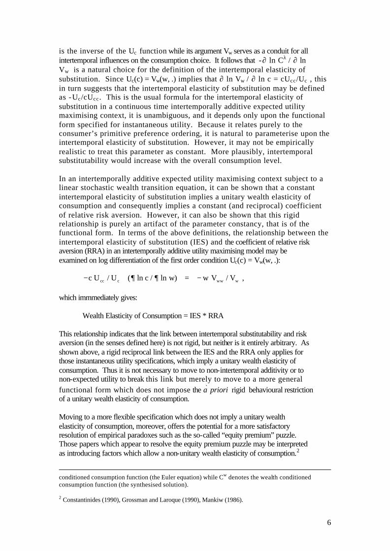
is the inverse of the Uc function while its argument Vw serves as a conduit for all intertemporal influences on the consumption choice. It follows that -∂ ln Cλ / ∂ ln Vw is a natural choice for the definition of the intertemporal elasticity of substitution. Since Uc(c) = Vw(w, .) implies that ∂ ln Vw / ∂ ln c = cUcc/Uc , this in turn suggests that the intertemporal elasticity of substitution may be defined as -Uc/cUcc. This is the usual formula for the intertemporal elasticity of substitution in a continuous time intertemporally additive expected utility maximising context, it is unambiguous, and it depends only upon the functional form specified for instantaneous utility. Because it relates purely to the consumer’s primitive preference ordering, it is natural to parameterise upon the intertemporal elasticity of substitution. However, it may not be empirically realistic to treat this parameter as constant. More plausibly, intertemporal substitutability would increase with the overall consumption level. In an intertemporally additive expected utility maximising context subject to a linear stochastic wealth transition equation, it can be shown that a constant intertemporal elasticity of substitution implies a unitary wealth elasticity of consumption and consequently implies a constant (and reciprocal) coefficient of relative risk aversion. However, it can also be shown that this rigid relationship is purely an artifact of the parameter constancy, that is of the functional form. In terms of the above definitions, the relationship between the intertemporal elasticity of substitution (IES) and the coefficient of relative risk aversion (RRA) in an intertemporally additive utility maximising model may be examined on log differentiation of the first order condition Uc(c) = Vw(w, .): − = −c U / U ( ln c / ln w) w V / Vcc c ww w∂ ∂ , which immmediately gives: Wealth Elasticity of Consumption = IES * RRA This relationship indicates that the link between intertemporal substitutability and risk aversion (in the senses defined here) is not rigid, but neither is it entirely arbitrary. As shown above, a rigid reciprocal link between the IES and the RRA only applies for those instantaneous utility specifications, which imply a unitary wealth elasticity of consumption. Thus it is not necessary to move to non-intertemporal additivity or to non-expected utility to break this link but merely to move to a more general functional form which does not impose the a priori rigid behavioural restriction of a unitary wealth elasticity of consumption. Moving to a more flexible specification which does not imply a unitary wealth elasticity of consumption, moreover, offers the potential for a more satisfactory resolution of empirical paradoxes such as the so-called “equity premium” puzzle. Those papers which appear to resolve the equity premium puzzle may be interpreted as introducing factors which allow a non-unitary wealth elasticity of consumption.2

conditioned consumption function (the Euler equation) while Cw denotes the wealth conditioned consumption function (the synthesised solution). 2 Constantinides (1990), Grossman and Laroque (1990), Mankiw (1986).

7

Those papers which appear unable to resolve the puzzle, even if they break the link between alleged measures of risk aversion and intertemporal substitutability, generally retain a unitary wealth elasticity of consumption.3 Consideration of the issues raised above suggests that it would be worthwhile to explore the specification of functional forms which do not imply a unitary wealth elasticity. These forms allow recognition of some of the issues which in the quoted literature are raised as important, such as the requirement for a more flexible but intuitively reasonable relationship between intertemporal substitutability and risk aversion, without abandoning either the intertemporal additivity assumption or the expected utility paradigm. 3. Notation, Assumptions and Preliminary Results In this section a general methodology is proposed to enable the examination of intertemporal substitutability and risk aversion in a representative consumer/firm context. For the purpose of allowing the theoretical specification to represent the microfoundations of a macro model, the aggregate consumption variable is generalised beyond simply consumer aggregate expenditure to represent the “full” expenditure of a representative consumer/firm, and the transition equation is generalized to allow nonlinear technology and to represent the national income identity. The analysis concentrates on the real open economy. Monetary factors are not considered but the model is developed in an explicit two-country context – a home and a foreign country – where the second country could be interpreted either as a major trading partner with other partners exogenous, or possibly as an aggregate of the rest of the world. Define )(zU as the home country representative consumer/firm’s instantaneous utility function, where z is an aggregate of real consumption, net exports and balancing items, representing total current expenditure in the national income identity. Ignoring minor items such as depreciation and valuation adjustments, essentially xcz += where c is real consumption and x is net exports. The representative agent derives instantaneous utility not only from current consumption but also from the implications of net exports in terms of foreign debt reduction or foreign exchange accumulation.

)(zU is interpreted as an indirect utility function. Its dependence on the relative prices of c and x is suppressed for convenience as attention is concentrated on intertemporal aspects of the optimization problem. The budgeting process is essentially two stage. While optimal c and x - conditional on aggregate expenditure z - could be determined by Roy’s Identity applied to )(zU , the following analysis concentrates on the intertemporal choice between z and investment in the country’s capital stock. It is assumed that 0)( >zU z , 0)( <zU zz , where single (double) subscripts denote first (second) derivatives respectively. Let *)(* zU denote the foreign country 3 Weil (1989), Attanasio and Weber (1989), Kocherlakota (1990). See also the survey articles by Abel (1991) and Kocherlakota (1996).

8

representative agent’s utility function, which will be subject to analogous assumptions. The home and foreign countries’ representative consumer-firms’ optimisation problems are linked in the sense that each acts under constraints arising from the evolution of variables which are determined as the outcome of the optimization problem of the other. It is assumed that in each case the representative agent acts as if it is in a competitive situation in which its decision making does not affect that of the agent in the other country. In fact, this competitiveness assumption will be strengthened to facilitate derivations below. The optimal value functions implied by the optimisations may be defined by:

∫∞ −

∞=00)(),(

))((max),*,,(0

dttzUeEskkJ ttatz

δµ (1a)

∫∞ −

∞=0

*0)*(),*(

))(*(*max*),/1,*,(*0

dttzUeEskkJ ttatz

δµ (1a*)

subject to the constraints:

)()()()()())(()( 2 tdtadttztattkFtdk ξσγσ +−+= (1b)

)(*)(**)(*)(*)(**)(*(*)(* 2 tdtadttztattkFtdk ξσγσ +−+= (1b*)

[ ]2

)(/))(()(*/))(*(*1)()(

σχµγ tktkFtktkFt

t−+= (1c)

[ ] [ ]

2*

)(*/))(*(*)(/))((*1)(/1)(*

σ

χµγ

tktkFtktkFtt

−+= (1c*)

)()( tdtd µµ ξσµ = (1d)

kk =)0( (1e)

*)0(* kk = (1e*)

µµ =)0( (1f) where (assumed constant) parameters are collected for notational convenience from the perspective of the objectives of the two countries as:

)*,*,,,*,,( ′= δδχχσσσ µs , )*,,*,,,*,(* 2 ′= δδχχσµσσ µs .

9

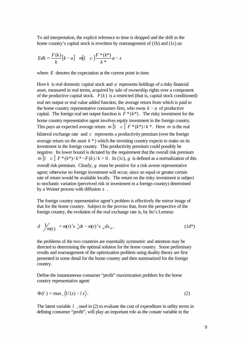
To aid interpretation, the explicit reference to time is dropped and the drift in the home country’s capital stock is rewritten by rearrangement of (1b) and (1c) as:

[ ] [ ] zak

kFak

kkF

Edk −++−=*

*)(*1

)( χµ

where E denotes the expectation at the current point in time. Here k is real domestic capital stock and a represents holdings of a risky financial asset, measured in real terms, acquired by sale of ownership rights over a component of the productive capital stock. F k( ) is a restricted (that is, capital stock conditioned) real net output or real value added function, the average return from which is paid to the home country representative consumer-firm, who owns ak − of productive capital. The foreign real net output function is *)(* kF . The risky investment for the home country representative agent involves equity investment in the foreign country. This pays an expected average return [ ] */*)(*1 kkFχµ + . Here µ is the real

bilateral exchange rate and χ represents a productivity premium (over the foreign average return on the asset *k ) which the investing country expects to make on its investment in the foreign country. This productivity premium could possibly be negative. Its lower bound is dictated by the requirement that the overall risk premium

[ ] 0/)(*/*)(*1 >−+ kkFkkFχµ . In (1c), γ is defined as a normalization of this overall risk premium. Clearly, γ must be positive for a risk averse representative agent; otherwise no foreign investment will occur, since an equal or greater certain rate of return would be available locally. The return on the risky investment is subject to stochastic variation (perceived risk in investment in a foreign country) determined by a Weiner process with diffusion σ . The foreign country representative agent’s problem is effectively the mirror image of that for the home country. Subject to the proviso that, from the perspective of the foreign country, the evolution of the real exchange rate is, by Ito’s Lemma:

µµµ ξσµσµµ dtdtttd 223 )()()(1 −=

, (1d*)

the problems of the two countries are essentially symmetric and attention may be directed to determining the optimal solution for the home country. Some preliminary results and rearrangement of the optimization problem using duality theory are first presented in some detail for the home country and then summarized for the foreign country. Define the instantaneous consumer “profit” maximization problem for the home country representative agent:

zzUz λλ −=Φ )(max)( . (2) The latent variable λ , used in (2) to evaluate the cost of expenditure in utility terms in defining consumer “profit”, will play an important role as the costate variable in the

10

intertemporal optimization problem. The instantaneous optimization problem (2) has first order condition:

λ=)(zU z . (3) Importantly, optimal expenditure as a function of λ can be recovered from the optimized consumer profit function by Hotelling’s (envelope) theorem:

)(λλΦ−=z . (4) We note for later use that λ conditioned (“Frischian”) utility, defined by

))(()( 1 λλ −= zF UUU , may be constructed from the profit function on combination of

(4) with a rearrangement of (2) as:

)()()( λλλλ λΦ−Φ=FU . (5) Next, define the (optimized, current value, deterministic component of the) Hamiltonian:

)()(),( kFkH λλλ +Φ= . (6) Now define a latent variable, ρ say, to represent the implicit rental rate of capital. It can be shown that an appropriate measure of economy-wide economic profit is:

[ ] [ ]kkFzzUkz ρλλρλ −+−=Π )()(max),( , (7)

This follows from a definition of economy-wide economic profit obtained by combining consumer and producer profit, where producer profit is defined firstly as

kkFk ρ−)(max and then converted to utility terms by use of the scale factor λ . However, using (2) and (6), it will be convenient to work with the intermediate functions Φ and H in what follows. Thus, (7) is rewritten as:

kkHk ρλλρλ −=Π ),(max),( . (8) The concept of economy wide profit represented by (8) has many useful implications. We highlight four of them. Firstly, the first order condition for (8) implies ρλλ =),(kH k , which in view of (6) further implies:

)(kFk=ρ (9) and, in view of the assumption that 0<kkF , optimal k , denoted by k , may be written in terms of ρ as:

11

)(ˆ 1 ρ−= kFk . (10)

In cases where it is appropriate to make use of the competitiveness assumption – that the representative consumer-firm takes the aggregate average capital stock as given and contemporaneously optimal in the sense that arbitrage opportunities are exhausted and instantaneous profits are maximized – (10) allows the optimal capital stock to be explicitly eliminated in terms of the implicit rental rate ρ . Second, it is possible to rearrange (8) to translate the Hamiltonian into a form, conditioned on both λ and ρ , which is, very conveniently, linear affine in k :

kkH ˆ),(),,ˆ(ˆ ρλρλρλ +Π= . (11) Before proceeding, it is worth emphasising that the sense in which k is optimal here is that it is chosen to maximize instantaneous economic profits in a deterministic context in which capital is costed at the implicit rental rate ρ . If the representative agent has the option of an alternative safe investment at this rate of return, then the absence of arbitrage opportunities will be sufficient to ensure that k is contemporaneously optimal in the intertemporal problem. The assumption of absence of arbitrage opportunities is maintained here. With this assumption it will be possible

to replace k in (11) by the solution to a compatibly defined intertemporal optimization problem. Third, in view of (10) the average rate of return on holdings of productive assets can be defined in terms of ρ as:

)(

))(()(

1

1

ρρ

ρ−

−

=k

k

F

FFM . (12)

Similar concepts may be defined for the foreign country. Of particular relevance at this point are:

*)(** * kFk=ρ (9*)

*)(**ˆ 1* ρ−= kFk (10*)

*)(*

*))(*(**)(*

1*

1*

ρρ

ρ−

−

=k

k

F

FFM , (12*)

where **kF denotes the foreign marginal product function and 1

* *−kF denotes the

inverse function. Fourth, using the concepts of ρ and *ρ , the basic intertemporal optimization problems for the agents may be redefined, conditioned on the initial values of ρ , *ρ

12

and other exogenous explanators, as special cases of the more general optimization problems:

∫∞ −

∞=00)(),(

))((max),*,,*,,(0

dttzUeEskkJ ttatz

δµρρ (13a)

∫∞ −

∞=0

*0)*(),*(

))(*(*max*),/1,*,,*,(*0

dttzUeEskkJ ttatz

δµρρ (13a*)

subject to:

)()()()()()())(()( 2 tdtadttztattktMtdk ξσγσρ +−+= (13b)

)(*)(**)(*)(*)(**)(*))(*(*)(* 2 tdtadttztattktMtdk ξσγσρ +−+= (13b*)

[ ] )()()())(()()()())(())(()( 22

212 tdtadttatkFtztattkFtkFtd kkkkk ξσσγσρ ++−+=

(13c)

[ ]

)(*)(**

)(**))(*(*

)(*)(*)(**))(*(*))(*(*)(*

22***2

1

2**

tdta

dttatkF

tztattkFtkFtd

kkk

kk

ξσ

σ

γσρ

+

+

−+=

(13c*)

[ ]2

))(())(*(*1)()(

σρρχµγ tMtMt

t−+= (13d)

[ ] [ ]

2*

))(*(*))((*1)(/1)(*

σ

ρρχµγ

tMtMtt

−+= (13d*)

)()( tdtd µµ ξσµ = (13e)

kk =)0( (13f)

*)0(* kk = (13f*)

ρρ =)0( (13g)

*)0(* ρρ = (13g*)

µµ =)0( (13h)

13

and where, as before, )*,*,,,*,,( ′= δδχχσσσ µs , )*,,*,,,*,(* 2 ′= δδχχσµσσ µs . In the absence of initial arbitrage, defined by the additional requirement that the relationships between the initial conditions for the capital stock and its marginal product are given by (9) and (9*), problem (13) reduces to problem (1). It is convenient, however, to maintain the artificial separation of these initial conditions and work with the more general problem (13). At the same time, attention is restricted to the competitive optimizations implied by the assumption that the representative agent in each country takes the paths of ρ and *ρ as exogenously given, though optimal. It is clear from the structure of problem (13) that optimal solutions for **,,, azaz in synthesized form, if they exist, may be written in terms of the contemporaneous values of the predetermined variables µρρ *,,*,,kk and the parameter vector s . Let:

),*,,(ˆ),*,,*,,(ˆ sZskkZz µρρµρρ == (14a)

),*,,(ˆ),*,,*,,(ˆ sAskkAa µρρµρρ == (14b)

),*,,(*ˆ*),/1,*,,*,(**ˆ sZskkZz µρρµρρ == (14a*)

),*,,(*ˆ*),/1,*,,*,(**ˆ sAskkAa µρρµρρ == (14b*) denote the optimal competitive solutions, that is, the solutions for the choice variables if the home and foreign country representative agents take the paths of ρ and *ρ as exogenously given but consistent with their optimal choices, and where the second equality in each of (14) uses (10) and (10*). To aid presentation, let us further define:

))(()( 10 ρρ −≡ kFFN , ))(()( 12 ρρ −≡ kkk FFN , ))(()( 13 ρρ −≡ kkkk FFN (15)

*))(*(**)(* 1*

0 ρρ −≡ kFFN , *))(*(**)(* 1***

2 ρρ −≡ kkk FFN ,

*))(*(**)(* 1****

3 ρρ −≡ kkkk FFN (15*) Problem (13) may then be decoupled into separate home country and foreign country decision making problems. The home country problem is:

∫∞ −

∞=00)(),(

))((max),*,,*,,(0

dttzUeEskkJ ttatz

δµρρ (16a)

subject to:

)()()()()()())(()( 2 tdtadttztattktMtdk ξσγσρ +−+= (16b)

)(*)(*ˆ*)(*ˆ)(*ˆ)(**)(*))(*(*)(* 2 tdtadttztattktMtdk ξσγσρ +−+=

(16c)

14

[ ] )()(ˆ

)(ˆ))(()(ˆ)(ˆ)())(())(()( 2232

1202

tdta

dttatNtztattNtNtd

ξσσργσρρρ

++−+=

(16d)

[ ]

)(*)(*ˆ*

)(*ˆ*))(*(*

)(*)(*ˆ)(**))(*(*))(*(*)(*

2232

1

202

tdta

dttatN

tztattNtNtd

ξσσρ

γσρρρ

+

+

−+=

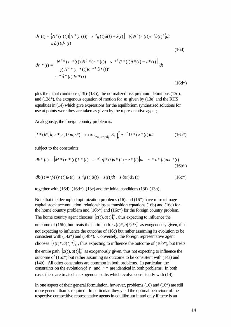
(16d*) plus the initial conditions (13f)-(13h), the normalized risk premium definitions (13d), and (13d*), the exogenous equation of motion for µ given by (13e) and the RHS equalities in (14) which give expressions for the equilibrium synthesized solutions for use at points were they are taken as given by the representative agent; Analogously, the foreign country problem is:

∫∞ −

∞=0

*0)*(),*(

))(*(*max*),/1,*,,*,(*0

dttzUeEskkJ ttatz

δµρρ (16a*)

subject to the constraints:

)(*)(**)(*)(*)(**)(*))(*(*)(* 2 tdtadttztattktMtdk ξσγσρ +−+= (16b*)

)()(ˆ)()(ˆ)()())(()( 2 tdtadttztattktMtdk ξσγσρ +−+= (16c*)

together with (16d), (16d*), (13e) and the initial conditions (13f)-(13h). Note that the decoupled optimization problems (16) and (16*) have mirror image capital stock accumulation relationships as transition equations (16b) and (16c) for the home country problem and (16b*) and (16c*) for the foreign country problem.

The home country agent chooses ∞0)(),( tatz , thus expecting to influence the

outcome of (16b), but treats the entire path ∞0*)()*,( tatz as exogenously given, thus

not expecting to influence the outcome of (16c) but rather assuming its evolution to be consistent with (14a*) and (14b*). Conversely, the foreign representative agent

chooses ∞0*)()*,( tatz , thus expecting to influence the outcome of (16b*), but treats

the entire path ∞0)(),( tatz as exogenously given, thus not expecting to influence the

outcome of (16c*) but rather assuming its outcome to be consistent with (14a) and (14b). All other constraints are common in both problems. In particular, the constraints on the evolution of ρ and *ρ are identical in both problems. In both cases these are treated as exogenous paths which evolve consistently with (14). In one aspect of their general formulation, however, problems (16) and (16*) are still more general than is required. In particular, they yield the optimal behaviour of the respective competitive representative agents in equilibrium if and only if there is an

15

absence of initial arbitrage opportunities. Thus, the equilibrium requires that the synthesized solutions for (16) and (16*) have superimposed upon them the contemporaneous constraints (9) and (9*). 4. Solution of the Intertemporal Optimisation This section presents the solution to problem (16) and, by analogy, the solution to the mirror image problem (16*), in a form capable of adaptation to econometric estimation of the model equations for quite general preference and technology specifications. The Hamilton-Jacobi-Bellman (HJB) equation for the home country representative competitive agent problem (16), constructed by Bellman’s Principle of Optimality, involves the representative agent making a trade-off between the acquisition of utility from current expenditure and the acquisition of potential for additional utility in future as an outcome of capital accumulation. The decision making is undertaken by the competitive agent given that what is believed to be under its influence is the expected path of k , but not that of *k , ρ , *ρ or µ . It is

assumed that the Weiner processes )(tdξ , )(* tdξ and )(td µξ are independent and that the representative competitive agent makes decisions consistently with the correctly evolving value of ))(( ρddkE but in the belief that the value of this covariance is not affected by individual optimization decisions. Note also that

0)( =tEdµ for simplicity, though this is inconsequential. Under these conditions, the HJB equation for the competitive optimum for the home country is:4

+

+++

+++

+++

+

=

22

1

22

12**2

122

1

2**2

1**

**

,

)(

)(*)()(

*)(*)*)(())((

*)()(*)()(

1)(max

),*,,*,,(

dkEJ

dEJdEJdEJ

dkEJddkEJddkEJ

dEJdEJdkEJdkEJ

dtzU

skkJ

kk

kkkk

kk

azµρρ

ρρ

ρρ

µρρδ

µµρρρρ

ρρ

ρρ

(17)

where the mean expectations, covariances and variances may be calculated from the assumptions and the relationships (16b), (16c), (16d) , (16d*) and (13e) as:

zakMdkEdt

−+= γσρ 2)()(1

(18a)

),*,,(*ˆ),*,,(*ˆ***)(*)(1 2 sZsAkMdkEdt

µρρµρργσρ −+= (18b)

4 The assumptions on the independence of the Weiner processes imply that

0)*)((,0)*)((,0))((,0*))((,0*))(( ===== µρµρ ddkEddkEddkEddkEdkdkE . These restrictions, in addition to the structural assumption on zero drift in the real exchange rate, are imposed in (17). The assumption on the exogeneity of the covariance ))(( ρddkE from the point of

view of the optimization decision of the representative competitive agent is reflected in the use of (14b) in (18e) below.

16

[ ][ ]223

21

202

),*,,(ˆ)(

),*,,(ˆ),*,,(ˆ)()()(1

sAN

sZsANNdEdt

µρρσρ

µρρµρργσρρρ

+

−+= (18c)

[ ][ ]223

21

202

),*,,(*ˆ**)(*

),*,,(*ˆ),*,,(*ˆ***)(**)(**)(1

sAN

sZsANNdEdt

µρρσρ

µρρµρργσρρρ

+

−+= (18d)

[ ]222 ),*,,(ˆ)())((1

sANddkEdt

µρρσρρ = (18e)

[ ]222 ),*,,(*ˆ**)(**)*)((1

sANddkEdt

µρρσρρ = (18f)

[ ]222 ),*,,(*ˆ**)(1

sAdkEdt

µρρσ= (18g)

[ ] [ ]22222 ),*,,(ˆ)()(1

sANdEdt

µρρσρρ = (18h)

[ ] [ ]22222 ),*,,(*ˆ**)(**)(1

sANdEdt

µρρσρρ = (18i)

22)(

1µσµ =dE

dt (18j)

222)(

1adkE

dtσ= (18k)

Given (18), the first order conditions for (17) are:

kz JzU =)( (19) and

kkk JJa /γ−= (20) and, using (2), (3) and (6), this allows the (optimized from the viewpoint of the representative competitive agent) HJB equation implied by (17) to be written as:

ωγσδ +−= kkkk JJJkHJ /),( 2222

1 (21) where:

17

++++

++++=

22

12**2

122

12**2

1

****

)(*)()(*)(

*)*)(())((*)()(*)(1

µρρ

ρρρρω

µµρρρρ

ρρρρ

dEJdEJdEJdkEJ

ddkEJddkEJdEJdEJdkEJ

dtkk

kkk(22)

Using (10) and (10*) to eliminate k and *k from the partial derivative expressions, and substituting in the relevant terms from (18), an explicit though complex expression for the term ω which depends explicitly only on µρρ *,, and s may be obtained and summarized as:

),*,,( sµρρω Ω= . (22’) The objective of this section is to rewrite the HJB equation in a form which ultimately provides a source of endogenisation of the costate variable λ . In order to complete this task, use is made of the optimal value function, treating it as “output” and defining its dual, optimal intertemporal profit. Concentrating on the home country optimization in what follows, it will be convenient and involve no loss of generality to use (10*) to eliminate *k in terms of *ρ and define:

),*,,*),(*,(),*,,,(ˆ 1* sFkJskJ k µρρρµρρ −≡ . (23)

Dual to problem (16) is the following “intertemporal profit” maximizing problem:

kskJs k λµρρµρρλ −=Ψ ),*,,,(ˆmax),*,,,( (24)

which implies, consistently with (19) and (2), and hence ultimately with (1) under the additional condition of competitive decision making, the first order condition:

λµρρ =),*,,,(ˆ skJ k . (25) An envelope result (Hotelling’s Theorem) gives:

),*,,,( sk µρρλλΨ−= . (26) Together, (25) and (26) yield an identity:

λµρρµρρλλ ≡Ψ− ),*,,),,*,,,((ˆ ssJ k , (27) differentiation of which further implies:

λλΨ−= /1ˆkkJ . (28)

Using (25) and (28), optimal foreign asset holdings may be written as:

λλγλΨ=a (29)

18

Additionally, using (25), (24) may be rearranged to give a costate conditioned form of the optimal value function:

),*,,,(),*,,,(),*,,,(~

sssJ µρρλλµρρλµρρλ λΨ−Ψ= (30) Then, using (11), (25), (28) and (30), the HJB equation (21) may be rewritten in terms of the intertemporal profit function Ψ as:

[ ]),*,,(),*,,,(

),*,,,(),(),*,,,(),*,,,(222

21 ss

sss

µρρµρρλλγσ

µρρλρλρλµρρλλµρρλδ

λλ

λλ

Ω+Ψ+

Ψ−Π=Ψ−Ψ

(31) a second order linear differential equation which may be explicitly solved for Ψ . Assuming 0≠σ , as is natural for the stochastic case, the solution of (31) can be verified by direct examination to be (see Cooper (1999) and Cooper (2000) for more details on the deterministic and stochastic cases, respectively):

[ ] δµρρ

ββγσ

ζρζζλζρζζλλ

λ

ββββ),*,,(),(),(

1222

21

0

11 2211sdd Ω+

−

Π+Π=Ψ ∫ ∫

∞ −−−−

(32)

where:

22

2

22

222

1

22

222

1

1

2γσδ

γσγσδρ

γσγσδρβ +

+−−+−= (33a)

22

2

22

222

1

22

222

1

2

2γσδ

γσγσδρ

γσγσδρβ +

+−++−= (33b)

The requirement that the integrals in (32) converge to finite values effectively imposes the transversality condition for the optimization. This imposes parameter restrictions on the function Π and hence on the underlying preferences and technology which need to be checked for specific functional form specifications. For development of the model it is useful to employ (30) together with (32) to generate an expression for the optimal value function. As an aid to simplification, it is first noted that, by an envelope theorem applied to (8) and use of (6):

kkF ˆ)ˆ()(),( ρλρλ λλ −+Φ=Π where k is the optimal solution of (6), itself a function of λ and ρ . Then, comparing this result with (6) and (8), it may be noted that:

19

)()(),(),( λλλρλλρλ λλ Φ−Φ=Π−Π , (34) an expression which eliminates ρ and which, by virtue of (5), may be seen to represent costate conditioned, or Frischian, instantaneous utility. Now, integrating RHS (32) by parts and using (30) and (34), the optimal value function may be derived in a form conditioned on λ and ρ as:

[ ] [ ][ ]

δµρρ

ββγσ

ζζζζζλζζζζζλµρρλ

λ

λ λββ

λββ

),*,,(

)()()()(),*,,,(

~

1222

21

0

11 2211

s

ddsJ

Ω+

−

Φ−Φ+Φ−Φ= ∫ ∫

∞ −−−−

(35) In order to collect the complete set of model equations into a coherent form, it is useful to record some ancillary results. Firstly, defining a latent variable, j say, to represent the endogenous (to the decision maker) component of the optimal value function, we have:

),*,,,(~),*,,(

),*,,,(~ 0 sJ

ssJj µρρλ

δµρρµρρλ =Ω−= . (36)

In what follows (36) will be referred to as the truncated optimal value function. It may be noted for later reference that the truncated optimal value function is capable of explicit evaluation by integrating the term on the top line of (35). Moreover, by combining (30) and (36) with the HJB equation (31), in view of (6), (8), (27), and (29) a (non-linear) equation for the costate variable may be written as a rearrangement of the HJB equation:

akFj

γσλδλ

22

1)()(

+Φ−= (37)

Additionally, from (25), (26) and (28), the Arrow-Pratt coefficient of relative risk aversion may be characterized as:

λλλΨ=−= k

JkJr kkk / (38)

and, in terms of the risk aversion coefficient, the risky asset choice (29) may be represented as:

kr

aγ= . (39)

In bringing together these results some further latent variables are defined to simplify expressions. These additional definitions, and their relationships to the results derived

20

above, are explained following a listing of the full set of equations for the home country component of the model, which is set out below.

)(kFf = (40a)

)(kFk=ρ (40b)

[ ]2

/*/*1

σ

χµγ

kfkf −+= (40c)

22

2

22

222

1

22

222

1

1

2γσδ

γσγσδρ

γσγσδρβ +

+−−+−= (40d)

22

2

22

222

1

22

222

1

2

2γσδ

γσγσδρ

γσγσδρβ +

+−++−= (40e)

)(λφ Φ= (40f)

[ ] [ ][ ] 22222

21

1

0

1

2

)()()()( 2211

γδσγσδρ

ζζζζζλζζζζζλλ λ

ββλ

λββ

++−

Φ−Φ+Φ−Φ= ∫∫

∞ −−−− ddj (40g)

[ ][ ] [ ]∫∫

∞ −−−−−− Φ−Φ+Φ−Φ

++−−=

λ λββλ

λββ ζζζζζλβζζζζζλβ

γδσγσδρ

dd

kr

)()()()(

211

20

111

222222

1

2211

(40h)

kr

aγ= (40i)

af

j

γσ

φδλ

22

1+

−= (40j)

)(λλΦ−=z (40k)

ζσγσ addtzafdk +−+= 2 (40l)

Equation (40a) represents some general specification of technology for the home country. Real output is represented by a latent variable f and is modeled as a

21

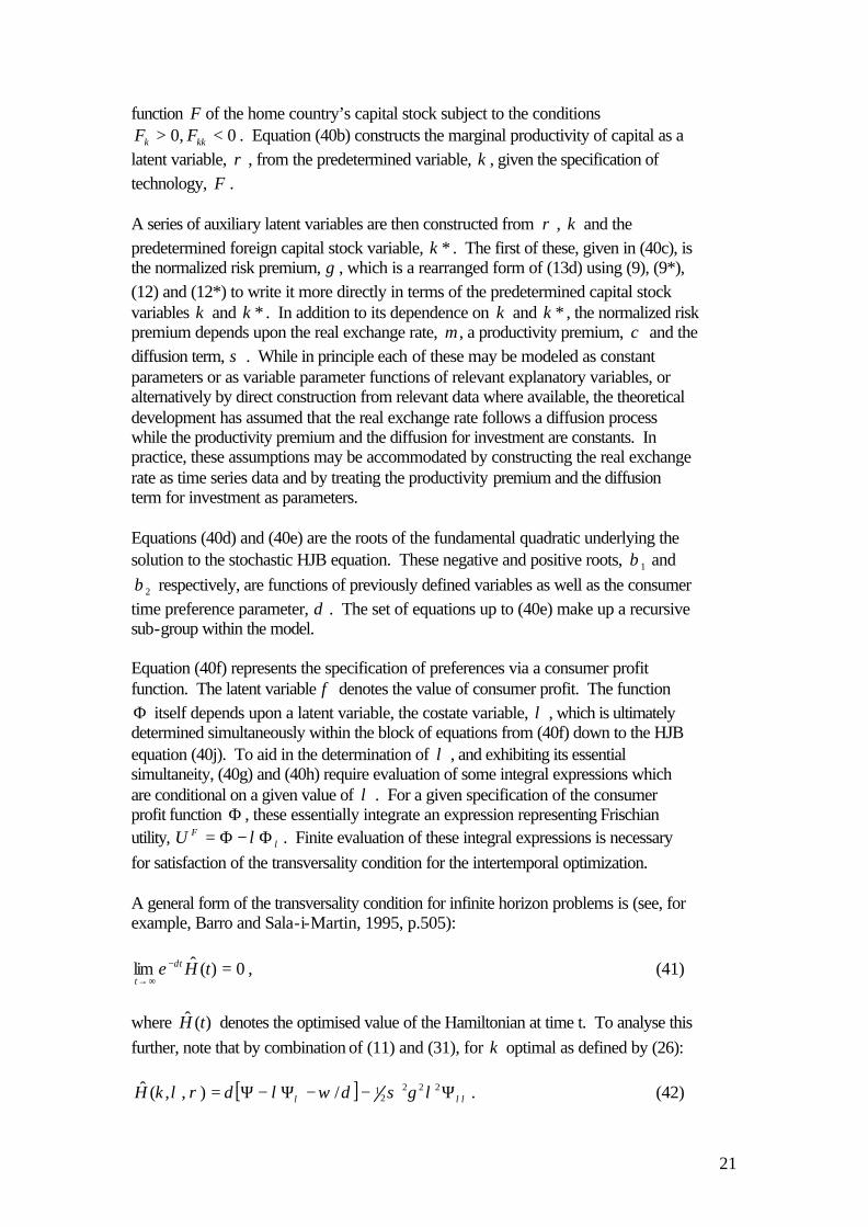
function F of the home country’s capital stock subject to the conditions 0,0 <> kkk FF . Equation (40b) constructs the marginal productivity of capital as a

latent variable, ρ , from the predetermined variable, k , given the specification of technology, F . A series of auxiliary latent variables are then constructed from ρ , k and the predetermined foreign capital stock variable, *k . The first of these, given in (40c), is the normalized risk premium, γ , which is a rearranged form of (13d) using (9), (9*), (12) and (12*) to write it more directly in terms of the predetermined capital stock variables k and *k . In addition to its dependence on k and *k , the normalized risk premium depends upon the real exchange rate, µ , a productivity premium, χ and the diffusion term, σ . While in principle each of these may be modeled as constant parameters or as variable parameter functions of relevant explanatory variables, or alternatively by direct construction from relevant data where available, the theoretical development has assumed that the real exchange rate follows a diffusion process while the productivity premium and the diffusion for investment are constants. In practice, these assumptions may be accommodated by constructing the real exchange rate as time series data and by treating the productivity premium and the diffusion term for investment as parameters. Equations (40d) and (40e) are the roots of the fundamental quadratic underlying the solution to the stochastic HJB equation. These negative and positive roots, 1β and

2β respectively, are functions of previously defined variables as well as the consumer time preference parameter, δ . The set of equations up to (40e) make up a recursive sub-group within the model. Equation (40f) represents the specification of preferences via a consumer profit function. The latent variable φ denotes the value of consumer profit. The function Φ itself depends upon a latent variable, the costate variable, λ , which is ultimately determined simultaneously within the block of equations from (40f) down to the HJB equation (40j). To aid in the determination of λ , and exhibiting its essential simultaneity, (40g) and (40h) require evaluation of some integral expressions which are conditional on a given value of λ . For a given specification of the consumer profit function Φ , these essentially integrate an expression representing Frischian utility, λλΦ−Φ=FU . Finite evaluation of these integral expressions is necessary for satisfaction of the transversality condition for the intertemporal optimization. A general form of the transversality condition for infinite horizon problems is (see, for example, Barro and Sala-i-Martin, 1995, p.505):

0)(ˆlim =−

∞→tHe t

t

δ , (41)

where )(ˆ tH denotes the optimised value of the Hamiltonian at time t. To analyse this further, note that by combination of (11) and (31), for k optimal as defined by (26):

[ ] λλλ λγσδωλδρλ Ψ−−Ψ−Ψ= 2222

1/),,(ˆ kH . (42)

22

Evaluating this using (32) gives:

[ ] 222222

1

12

222

10

11

222

1

2

)()()()(

),,(ˆ

2211

γδσγσδρ

ζζζλβγσδζζζλβγσδ

ρλ

λ

ββλ ββ

++−

+++

=

∫∫∞ −−−− dUdU

kH

FF

(43) Satisfaction of the transversality condition therefore requires two things in this context. First the integral expressions in (43) must be capable of finite evaluation. However, these are the same integral expressions involved in the model equations (40g) for the truncated optimal value function and (40h) for the coefficient of relative risk aversion. They need to be evaluated for choice of a specific functional form. Second, even if these expressions are finite for given t, there is a restriction on their growth over time along an optimal path. Clearly this will also depend upon the functional form specification. (40g) constructs the truncated optimal value, defined as that component of the value of the optimised objective which is under the control of the decision making economic agent, and denoted here by the latent variable j . Note that equation (40g) is an equivalent expression to the truncated optimal value function (36). In a similar manner, the Arrow-Pratt measure of relative risk aversion is constructed in (40h) as the latent variable r , by first deriving λλΨ from (32) and then applying this to (38). The risky asset choice is then given in (40i). Note that, no matter how complex the specification of preferences and technology, the proportion of resources held in the risky asset is simply the risk premium relative to the risk aversion coefficient. Finally, in (40j) the simultaneous loop determining the costate variable is closed by use of the HJB equation in the form (37), generatingλ as a latent variable. Given a value of λ determined by simultaneous solution of (40f)-(40j), equation (40k) then generates optimal current expenditure, z . This is then used along with previously determined variables to evaluate optimal investment in (40l). It should be noted that while data may be available on z , an alternative is to treat it as a latent variable. The same applies to the risky asset choice a and the real output variable f . The key equation ultimately is the growth equation (40l) and this is the only equation for which a stochastic disturbance term naturally arises from the theory. The equations for the foreign country are the mirror images of the set (40), with starred and unstarred variables interchanged. In the context of modeling two countries, the equation groups are linked through each country’s dependence on the evolution of the capital stock of the other. 5. Specification of the Home Country Component of the Model In this section the system (40) is set out for a particular specification of technology and preferences. The specification of preferences is chosen to contain the isoelastic utility specification as a special case. The technology specification contains the

23

typical power function specification as a special case. The general specifications are structured to enable investigation of the variability of the intertemporal elasticity of substitution (IES) and the Arrow-Pratt coefficient of relative risk aversion (RRA) over time and to examine empirically the nature of the relationship between them. In the following section a preliminary investigation is undertaken with South African data. 5.1 Preferences We choose the consumer profit function specification:

2

12

1

11

1)1(

1)(

21

ελεη

ελεηλ

εε

−−−+

−−=Φ

−−

(44)

where η , 1ε and 2ε are parameters, 10 << η and without loss of generality it may be assumed that ∞<≤< 210 εε . Implied optimal costate conditioned (Frischian) expenditure is, by (4):

21 )1()( εελ ληηλλ −− −+=Φ−=z (45)

and the intertemporal elasticity of substitution (IES) is:

IES = 21

21

)1()1(

log/log 21εε

εε

ληηλληεηλελ

−−

−−

−+−+=− dzd . (46)

In this specification, the IES is variable, being a weighted arithmetic mean of 1ε and

2ε , with weights which vary with the value of the costate variable. Given 21 εε < ,

when the representative consumer is poor and λ is large, 1ελ− dominates 2ελ− and IES 1ε→ . On the other hand, when the representative consumer is rich and λ is small, the reverse applies and IES 2ε→ . From (5), Frischian utility can be expressed as:

2

1

21

1

1 11

)1(1

1)()()(

21

ελεη

εληελλλλ

εε

λ −−−+

−−=Φ−Φ=

−−FU (47)

In the special case εεε == 21 , (44) corresponds to the isoelastic specification:

ελελ

ε

−−=Φ

−

1)(

1

(44’)

which implies:

ελ−=z , (45’) IES = ε (46’)

24

and

ελελ

ε

−−=

−

11

)(1

FU . (47’)

In this case the instantaneous utility function (in Marshallian form) is explicitly recoverable as:

ε

ε

/111

)(/11

−−=

−zzU .

Although an equivalent explicit expression for utility in Marshallian form is not recoverable under the more general specification (44), it is clear from (47) and (47’), where the representations in Frischian form may be compared, that utility for the representative agent in the general case (47) may be interpreted as a weighted average of the utility which would apply separately to the poor and the rich if the extreme poor and the extreme rich had separate isoelastic preferences with IES parameters 1ε and

2ε respectively. An important point about specification (44) is that the IES (46) is a variable and will ultimately be compatible, even in the intertemporally additive expected utility maximising context, with an Arrow-Pratt coefficient of relative risk aversion (RRA) which is not linked to it rigidly by reciprocality. This would be true even if the technology were specified to be linear. Another useful feature is that (45), by contrast with (45’) provides the prospect for considerably enhanced empirical fit. In two-country modeling, it would be natural to assume a similar preference specification for the foreign country. In the absence of evidence on cultural differences, there is no reason why preference parameters will differ at all and although this is trivial to generalise it would be interesting to assume in the first instance that the parameters 1ε and 2ε are identical in the two countries. That is, the extreme rich could be assumed to have similar preferences with respect to current versus future consumption in the two countries, and the same might reasonably apply across the two countries for the extreme poor. However, we allow the general preference specification of the representative consumer to be made up of a country-specific blend of these extremes, representing different wealth distributions. Of course, the costate variable will also, in general take a different value at any point in time in the two countries. The preference specification for the foreign country could therefore be represented as:

2

12

1

11

1*

*)1(1

***)(*

21

ελεη

ελεηλ

εε

−−−+

−−=Φ

−−

. (44*)

5.2 Technology We choose the specification:

25

[ ]

k

k

eekkk

kF−

−

+−+=

12

)(212

212θθθ ααα

. (48)

We assume 10 12 <≤≤ θθ , 210 αα ≤< . As 0→k the technology is dominated by

11)( θα kkF → , while as ∞→k it is dominated by 2

2)( θα kkF → . This function therefore nests standard specifications at its extremes and allows for more complex technology to apply for finite k . Under the parameter restrictions θθθ == 21 and

ααα == 21 , it reduces to the commonly employed power specification for all k ,

θαkkF =)( . (48’) If 021 == θθ , the function has the logistic form:

k

k

ee

kF−

−

+−+=

1)2(

)( 212 ααα. (48’’)

with )(kF ranging from 1α at 0=k to 2α as ∞→k . In the case of specification (48), the definition of ρ in (9) implies:

[ ] [ ]( )2

2122

11121

111

122

1

22)(

212112

k

kk

ke

ekkekkkkkF

−

−−−−−−

+

−++−+=θθθθθθ θαθαααθαθα

,

a result which is used to endogenise ρ as a latent variable in (58b) below. Given the generality of specification (48), the positivity of kF and, in an even more complex

fashion, the negativity of kkF (not displayed) will in general be parameter and data value dependent, and satisfaction of these restrictions may be checked as a test of the model empirically. Of course, in the special cases it is trivial to check that these restrictions will be automatically satisfied under the parameter value conditions specified above. It is convenient at this point to record the mirror image specification of technology for the foreign country in the two-country modeling case (with, of course, potentially different technological parameters):

[ ]*

**2

*1

*2

1****2**

*)(*212

k

k

eekkk

kF−

−

+−+=

θθθ ααα. (48*)

5.3 Integral evaluations and transversality conditions In order to employ specifications (44) and (48) to construct a specific model of the equation set (40) it is necessary to provide expressions for the evaluation of the integral expressions which are involved in (40g) and (40h) under specifications (44)

26

and (48). Utilising (47), it can be seen that these involve evaluation of expressions, 0i

and ∞i say, where:

ζε

ζεη

εζ

ηεζλ εε

β di ∫

−

−−+

−−

=−−

−−

02

1

21

1

11

0 11

)1(1

1 211 (49)

ζε

ζεη

εζ

ηεζλ

εεβ di ∫

∞ −−−−

∞

−

−−+

−−

=2

1

21

1

11

11

)1(1

1 212 (50)

Noting the definitions of 1β and 2β given in (40d) and (40e), it can be shown after considerable manipulation that:

011

2

2

222

21

22

2222

21

011

1

1

122

21

11

1222

21

2

2

1

1222

21

0

2121

1111

1

1)1(

))(1()1(

1))(1()1(

1)1(

1

=−−

=−−

=−−

=−−

−

−

−

−+−+

−−+

−

−+−+

−−+

−

−+−

=

ζεβ

λζεβ

ζεβ

λζεβ

β

ζζε

εηεγσρεδε

εβγσ

ζζε

εη

εγσρεδεεβγσ

λε

εη

εε

ηδ

βγσi

(49’)

In order for 0i to return a finite value it is necessary for the restrictions 01 11 >−− εβ

and 01 21 >−− εβ to ensure that the terms 01 11

=−−

ζεβζ and 0

1 21=

−−ζ

εβζ do not go to

infinity. Since 012 >≥ εε , a sufficient condition is the second of these, that involving 2ε , as this then implies satisfaction of the first. On manipulation of the definition of 1β the condition may be written:

( ) 0)1( 222

21

22 >+−+ εγσρεδε . (51) If 12 <ε this condition is necessarily satisfied. However, if 12 >ε the condition may be violated. Evaluating the positive root of the above quadratic, the condition may be written as:

22

2

2221

2221

2

2γσρ

γσρδ

γσρδε +

−++−+< . (52)

In a similar manner, it can be shown that:

27

λζεβ

ζεβ

λζεβ

ζεβ

β

ζζε

εηεγσρεδε

εβγσ

ζζε

εη

εγσρεδεεβγσ

λε

εη

εε

ηδ

βγσ

=−−

∞=−−

=−−

∞=−−

−∞

−

−

−+−+

−−−

−

−+−+

−−−

−

−+−

−=

2222

1212

2

11

2

2

222

21

22

2122

21

11

1

1

122

21

11

1122

21

2

2

1

1122

21

1)1(

))(1()1(

1))(1()1(

1)1(

1i

(50’)

In this case, to provide a finite value for ∞i it is necessary that the terms ∞=

−−ζ

εβζ 121

and ∞=−−

ζεβζ 221 do not explode. These conditions require 01 12 <−− εβ and

01 22 <−− εβ . Now, given 21 εε ≤ , satisfaction of the first condition implies the second. On manipulation of the definition of 2β , the condition can be written as:

( ) 0)1( 122

21

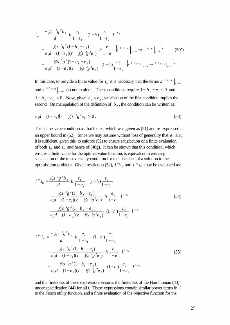
11 >+−+ εγσρεδε . (53) This is the same condition as that for 2ε which was given as (51) and re-expressed as an upper bound in (52). Since we may assume without loss of generality that 21 εε ≤ it is sufficient, given this, to enforce (52) to ensure satisfaction of a finite evaluation of both 0i and ∞i and hence of (40g). It can be shown that this condition, which ensures a finite value for the optimal value function, is equivalent to ensuring satisfaction of the transversality condition for the existence of a solution to the optimisation problem. Given restriction (52), 0

1iβλ and ∞i2βλ may be evaluated as:

2

1

1

1

2

2

222

21

22

2222

21

1

1

1

122

21

11

1222

21

2

2

1

1222

21

0

1)1(

))(1()1(

1))(1()1(

1)1(

1

ε

ε

β

λε

εηεγσρεδε

εβγσ

λε

εη

εγσρεδεεβγσ

εε

ηε

εη

δβγσ

λ

−

−

−

−+−+

−−+

−+−+

−−+

−

−+−

=i

(54)

2

1

2

1

2

2

222

21

22

2122

21

1

1

1

122

21

11

1122

21

2

2

1

1122

21

1)1(

))(1()1(

1))(1()1(

1)1(

1

ε

ε

β

λε

εηεγσρεδε

εβγσ

λε

εη

εγσρεδεεβγσ

εε

ηε

εη

δβγσ

λ

−

−

∞

−

−+−+

−−−

−+−+

−−−

−

−+−

−=i

(55)

and the finiteness of these expressions ensures the finiteness of the Hamiltonian (43) under specification (44) for all t. These expressions contain similar power terms in λ to the Frisch utility function, and a finite evaluation of the objective function for the

28

intertemporal optimization is therefore equivalent to satisfaction of the transversality condition. However, the finite value of the truncated optimal value function may actually be constructed, given restriction (52), as the evaluation of (40g) under specification (44). Specifically, in view of definitions (49) and (50), (40g) may be written:

( ) 22222

1

0

2

21

γδσγσδρ

λλ ββ

++−

+= ∞ii

j (56)

However, using (54) and (55) together with (40d) and (40e), (56) simplifies to:

+−+

−

−

−+

+−+

−

−

=

−

−

))(1(1

1)1(

))(1(1

1

222

21

22

1

2

2

122

21

11

1

1

1

2

1

εγσρεδελ

δεεη

εγσρεδελ

δεε

η

ε

ε

j

(56’)

In an analogous manner, for this specification equation (40h) becomes:

( )∞+++−−

=ii

kr

21201

22222

1 2ββ λβλβ

γδσγσδρλ. (57)

and once again using (54), (55), (40d) and (40e), this allows (57) to be simplified to:

))(1()1(

))(1( 222

21

22

2

122

21

11

121

εγσρεδελε

ηεγσρεδε

λεη

εε

+−+−+

+−+

=−−

kr (57’)

5.3 The complete model of the home country To summarise the specification under (44) and (48), the home country model equation system (40), treating relevant foreign country information as exogenous, becomes:

[ ]k

k

eekkk

f−

−

+−+=

12 212

212θθθ ααα

(58a)

[ ] [ ]( )2

2122

11121

111

122

1

22 212112

k

kk

e

ekkekkkk−

−−−−−−

+

−++−+=θθθθθθ θαθαααθαθαρ (58b)

[ ]2

/*/*1

σ

χµγ

kfkf −+= (58c)

29

22

2

22

222

1

22

222

1

1

2γσδ

γσγσδρ

γσγσδρβ +

+−−+−= (58d)

22

2

22

222

1

22

222

1

2

2γσδ

γσγσδρ

γσγσδρβ +

+−++−= (58e)

2

12

1

11

1)1(

1

21

ελεη

ελεηφ

εε

−−−+

−−=

−−

(58f)

+−+

−

−

−+

+−+

−

−

=

−

−

))(1(1

1)1(

))(1(1

1

222

21

22

1

2

2

122

21

11

1

1

1

2

1

εγσρεδελ

δεεη

εγσρεδελ

δεε

η

ε

ε

j

(58g)

))(1()1(

))(1( 222

21

22

2

122

21

11

121

εγσρεδελε

ηεγσρεδε

λεη

εε

+−+−+

+−+

=−−

kr (58h)

kr

aγ= (58i)

af

j

γσ

φδλ

22

1+

−= (58j)

21 )1( εε ληηλ −− −+=z (58k)

ξσγσ addtzafdk +−+= 2 . (58l)

30

6. Estimation To date we have been able to investigate the model empirically only in single-economy form for South Africa. The structural model of the “home country” elaborated above comprises a single equation of motion - a stochastic differential equation (SDE), equation (58l) - and several zero-order equilibrium relationships, equations (58a)-(58k). Under the assumption that ξd is a Wiener process, k is not differentiable. The equation of motion (58l), however, may be reinterpreted as an integral equation of the form:

∫∫ +−+=−tt

addtzafktk00

2)0()( ξσγσ (59)

Recognizing that LHS (59) is the flow of real net capital formation (or investment) over the interval dt , say [ ]tI ,0 , we can, by suitable redefinition and exchange of variables and rearrangement of terms, isolate the Wiener process on the right-hand side such that the investment equation can be solved numerically over a period of time in which 0.1=dt . Bergstrom (1997) and others have developed approaches to estimating systems of linear SDEs. We are not aware of any work in the econometrics literature on the estimation of systems of non-linear SDEs. But in view of the nature of the model, an existing non-linear estimation program of Wymer, discussed in Wymer (1993), may be used to obtain serviceable approximations to quasi-full-information-maximum-likelihood (quasi-FIML) estimates of the model's parameters. The adequacy of this approach in the present context remains to be evaluated. To estimate the model we use published annual data from 1980-1998 on GDP, capital formation and consumption, aggregates of non-investment items in national income identities, direct investment abroad, the rand/US$ exchange rate, and price deflators, for South Africa and “the industrial economies”, as reported on by the IMF, which stand in as “country two” or the rest of the world.5 The exact quasi-FIML non-linear continuous-time estimator of Wymer (1993) is implemented (in his program ESCONA) according to a two step algorithm. 1. For a given set of parameter estimates (or initial values) the equation system is integrated forward over each observation interval by a numerical variable-order, variable-step Adams method, residuals are computed by comparing the one-period-forward solution values with the observed values for variables on which there are

5 The data were obtained from various IMF and OECD publications. All real quantities were deflated by appropriate 1990 GDP price deflators. The real exchange rate was constructed by dividing the nominal rand/US$ exchange rate by the South African 1990 GDP price deflator and multiplying by the industrialized economies’ 1990 GDP price deflator. Series on capital stocks were constructed by the “perpetual inventory” method on base stocks that conform to the stylized facts of industrialized economies. Capital consumption is not reported for South Africa. We estimated this variable from the ratio of capital consumption to gross capital formation for the industrialized countries. This practice may introduce distortions in capital stock figures, but we deem it superior to the use of a constant percentage or an estimated depreciation parameter.

31

observations (for latent variables, of course, there will be none), and the variance covariance matrix is then formed. 2. The natural logarithm of the variance-covariance matrix is minimized by a quasi-Newton method to update parameter estimates. Convergence criteria are then checked and, if not met, another iteration is begun. Across-equation restrictions that are implied by theory are, of course, imposed in estimation. In estimating the model we have also imposed constraints on the values that parameters can assume. Estimates of all parameters must be non-negative, 1α

may not exceed 2α , 2θ may not exceed 1θ , 1ε may not exceed 2ε and η must be less than unity. The estimated model tracks the historical data very well with percentage root-mean-square errors of less than 3% in static in-sample forecasts of real variables. The quasi-FIML parameter estimates and the estimates of their asymptotic standard errors are given in Table 1.

Table 1: Preliminary Parameter Estimates6

Parameter Parameter Estimate Asymptotic Standard Error (Estimate)

1α 0.06574* 32.80894

2α 0.41837 0.09151

1θ 0.81758 0.08640

2θ 0.71596 0.08418

1ε 0.78652 0.01128

2ε 4.84622 0.10755 χ 1.08904 0.30624 δ 0.00001* 0.00007 η 0.98999 0.000003

2σ 0.14677 0.04288 There are several troubling aspects to the parameter estimates in Table1. Of most

concern is the estimate of the subjective time preference rate, δ , which is insignificantly different from zero. At the same time, the estimate of the asymptotic elasticity of substitution for the extremely wealthy, 2ε , is very large. As it turns out, the fact that 2ε is so large is not, in and of itself, a matter for concern. On the contrary, the very large difference between 1ε at 0.79 and 2ε at 4.85 is a matter of considerable interest, and points to a tendency in the data to support a variable elasticity of substitution which rises with wealth. The difficulty arises, however, with the transversality condition (51), which in view of the combination of these results turns out to be violated at all points in the sample. 6 * denotes an estimate not statistically discernible from zero at the 0.05 level of significance.

32

Possibly as a result of the violation of transversality, there is also a tendency in the parameter estimates for the influence of 2ε to be reduced. In fact, by virtue of the estimated value of η , which is insignificantly different from unity, the influence of

2ε is for all practical purposes eliminated. This reduces the preference specification virtually to the isoelastic form, in an apparent attempt to restore compatibility with the transversality condition which in the isoelastic case merely requires IES < 1. As will be discussed further below, for the current set of parameter estimates this attempt was not entirely successful and the model estimates remain incompatible with satisfaction of the transversality condition and hence with intertemporal optimisation. It would have been possible to maintain the more general preference specification compatibly with satisfaction of the transversality condition by enforcing a further restriction 2ε < 1. However, this would have done violence to what the data is saying. Our preferred option is to refine the data series, possibly investigate alternative generalisations of the isoelastic specification, and additionally conduct a more extensive search over a complex likelihood surface in what is a reasonably high dimensional parameter space. For present purposes, we continue the discussion conceding that the parameter estimate of 2ε is too high for comfort, that of δ is too low for comfort, that the combination of these violates transversality, that the closeness of the estimate of η to unity is an apparent attempt to redress this by enforcing isoelasticity, but that this compromise is not fully successful either. We turn now to the technology estimates and some additional overall implications of the combination of preference and technology estimates for the vaules of some key latent variables. We note firstly in passing (and discuss more fully below) that the results support the existence of a non-linear technology and hence (subject to the caveat of the preference parameter violations of optimality) the results tend to support a decoupling of strict reciprocality of the intertemporal elasticity of substitution (IES) and the Arrow-Pratt coefficient of relative risk aversion applied to resource risk (RRA). Results supporting the breaking of this link are reported in Table 2, where some key latent variables are presented as estimated over the final 10 years of the sample period.

Table 2: Time Series Estimates of Some Key Latent Variables

λ ρ IES RRA

1988 0.40019 0.14380 1.97911 1.98621 1989 0.40548 0.14311 1.93471 1.96419 1990 0.41795 0.14171 1.83619 1.89929 1991 0.42194 0.14070 1.80648 1.91020 1992 0.42011 0.14003 1.82001 1.96578 1993 0.41534 0.13951 1.85614 2.04495 1994 0.41836 0.13908 1.83310 2.03591 1995 0.42331 0.13832 1.79646 2.02801 1996 0.39510 0.13778 2.02336 2.42142 1997 0.39635 0.13723 2.01231 2.44064

33

As pointed out above, the implication of the parameter estimates, and of the closeness of η to unity in particular, is that the IES is virtually constant. Table 2 gives the calculation of this “constant” IES at approximately 2. This value is a weighted average of 0.78 and 4.85, using weights given in equation (46). These weights depend upon the value of the costate variable, λ , which has some small variation but is close to 0.4 on average over the examined time period. The large value of 2ε at 4.85 would have lead to considerable variation in the IES were it not for the negation of this effect by the multiplicative term )1( η− in (46). The equation for the RRA is given as one of the model’s latent variable equations, (58h). It is the second term in the denominator of (58h) which is problematic, as this term’s divisor, which should be positive in view of the transversality condition (51), is in fact negative due to the unfortunate combination of parameter estimates discussed above. Of course, in (58h) the multiplicative term )1( η− , being estimated as essentially zero, acts to reduce the influence of the transversality violating term (although, as conceded above, it does not do this completely successfully and consequently suggests that rationality is violated in the sense that the full set of necessary optimality conditions are not satisfied). As noted above (and subject to the caveat of the violation of rationality), the implied IES is virtually constant. Despite this, the RRA is very clearly not equal to the reciprocal of the IES. Examination of the formulae for the IES and the RRA (and a rather complex expression for the capital elasticity of expenditure which is implied by (58k) together with the simultaneous solution of (58a)-(58j) which theoretically provides λ as a function of k ) shows that this lack of reciprocality is due to the divergence of the technology from linearity rather than to the violation of rationality. That is, for the specifications considered here, the capital elasticity of expenditure (which is the natural analogue in the representative consumer-firm context of the wealth elasticity of consumption discussed in Section 2) is decidedly non-unity. The technology estimates are rather interesting in their own right. As can be seen by referring back to Table 1, the estimate of the parameter 1α is clearly insignificantly different from zero. This implies that too much was expected from the data in trying to determine with precision the shape of the power function for technology at 0=k . All that the data is saying at this point is that 0)0( =F , which is at least comforting.

However, the results have more to say asymptotically, where the estimates of 2α and

2θ imply that:

72.042.0)( kkF → as ∞→k . Subject to a caveat on the precision of estimation of the asymptotic standard error of

2θ , the technology appears to be significantly different from linear asymptotically. It

is also non-linear for finite k . In fact, setting 1α to zero as is implied strongly by the data, the best estimate of the production function for finite k is:

34

+−

= −

−

k

k

ee

kkF11

42.0)( 72.0

It is this non-linearity which produces estimates of a relatively high degree of risk aversion compatibly with a high degree of intertemporal substitutability. These kinds of results can help in explaining the equity premium paradox because they can justify a high equity premium to provide recompense for high risk aversion at the same time as they allow a substantial willingness to substitute current for future consumption. 7. Conclusion In this paper we have sought to provide the theoretical background to an examination of the relationship between volatility and growth from a representative agent modelling perspective. We have argued firstly that the issues may be fruitfully examined within the context of the intertemporally additive expected utility maximising paradigm, provided that sufficiently general functional forms are employed. We have then proposed and developed at some length a methodology based on reasonably extensive use of results in duality theory to enable the complete derivation of estimating forms which are consistent with these microeconomic foundations. Finally, we have undertaken a preliminary empirical investigation using South African data. The issue of the relative weight which policy makers should give to reduction in variability at the apparent expense of growth versus opting for growth at the apparent expense of variability is one of vital importance to many countries, but particularly to countries which are at crucial stages of economic and social development such as South Africa. The microeconomic perspective enables the conflicting criteria to be examined in an overall consistent framework under a utility maximising objective in which welfare variations due to policy changes can be explicitly examined. The preliminary estimates obtained and discussed in this paper suggest that the proposed methodology can provide a viable means of addressing these important issues. It also points, however, to the need for an ongoing effort to refine the data and to generalise to a point of empirical satisfaction the types of preference relationships and technologies which are specified and maintained behind these types of relatively sophisticated microeconomic foundations based analyses. The methodology described in this paper has been researched and purpose built precisely to enable generalisations of the tightly theoretically specified functional forms which are now current in the theoretical growth literature in order to align them more closely with the probably more flexible specifications which will be required to offer practical input to the policy debate. The reported results are mixed but they point clearly to a promising research path.

35

References Abel, A.B., (1991), “The Equity Premium Puzzle”, Business Review: Federal Reserve Bank of Philadelphia, Sept/Oct, 3-14. Attanasio, O.P. and G. Weber, (1989), “Intertemporal Substitution, Risk Aversion and the Euler Equation for Consumption”, The Economic Journal, 99, 59-73. Barro, R.J. and X. Sala-i-Martin, (1995), Economic Growth, McGraw-Hill. Bergstrom, A.R., (1997) "Gaussian Estimation of Mixed-Order Continuous-Time Dynamic Models with Unobservable Stochastic Trends from Mixed Stock and Flow Data," Econometric Theory, 13, 467-505. Browning, M., (1982), “Profit Function Representations for Consumer Preferences”, Discussion Paper 82/125, Bristol University. Browning, M., A. Deaton and M. Irish, (1985), “A Profitable Approach to Labor Supply and Commodity Demands over the Life Cycle”, Econometrica, 53:3, 503-543. Constantinides, G.M., (1990), “Habit Formation: A Resolution of the Equity Premium Puzzle”, Journal of Political Economy, 98: 3, 519-543. Cooper, R.J., (1999), “General Structural Dynamic Economic Modelling”, Paper presented to 28th Conference of Economists, La Trobe University, Melbourne, Australia, 26-30 September. Cooper, R.J., (2000), “An Approach to the Solution of Stochastic Growth Models with Generalised Preference and Technology Specifications”, manuscript in preparation. Deaton, A., (1992), Understanding Consumption, Clarendon Lectures in Economics, Oxford University Press. Epstein, L.G. and S.E. Zin, (1989), “Substitution, Risk Aversion, and the Temporal Behavior of Consumption and Asset Returns: A Theoretical Framework”, Econometrica, 57: 4, 937-969. Epstein, L.G. and S.E. Zin, (1991), “Substitution, Risk Aversion, and the Temporal Behavior of Consumption and Asset Returns: An Empirical Analysis”, Journal of Political Economy, 99: 2, 263-286. Grossman, S.J. and G. Laroque, (1990), “Asset Pricing and Optimal Portfolio Choice in the Presence of Illiquid Durable Consumption Goods”, Econometrica, 58: 1, 25-51. Kocherlakota, N.R., (1990), “The Equity Premium: It’s Still a Puzzle”, Journal of Economic Literature, XXXIV (1996), 42-71. Lucas, R.E., Models of Business Cycles, Yrjo Johnsson Lectures, Helsinki (1987), Oxford: Basil Blackwell (1987).

36

Lucas, R.E., (1988), “On the Mechanics of Economic Development”, Journal of Monetary Economics, 22, 3-42. Mankiw, G.N., (1986), “The Equity Premium and the Concentration of Aggregate Shocks”, Journal of Financial Economics, 17, 211-219. Mehra, R. and E.C. Prescott, (1985), “The Equity Premium: A Puzzle”, Journal of Monetary Economics, 15, 145-161. Naik, N.Y. and M.J. Moore, (1996), “Habit Formation and Intertemporal Substitution in Individual Food Consumption”, Review of Economics and Statistics, LXXVIII, 321-328. Obstfeld, M., (1994), “Evaluating Risky Consumption Paths: The Role of Intertemporal Substitutability”, European Economic Review, 38, 1471-1486. Pratt, J.W., (1964), “Risk Aversion in the Small and in the Large”, Econometrica, 32: 1-2, 122-136. Ramey, G. and V.A. Ramey, (1995), “Cross-Country Evidence on the Link Between Volatility and Growth”, American Economic Review, 85: 5, 1138-1151. Romer, P.M., (1986), “Increasing Returns and Long-Run Growth”, Journal of Political Economy, 94:5, 1002-1037. Turnovsky, S.J., (1995), Methods of Macroeconomic Dynamics, Cambridge, Ma.: MIT Press. Weil, P., (1989), “The Equity Premium Puzzle and the Risk-Free Puzzle”, Journal of Monetary Economics, 24, 401-421. Weil, P., (1990), “Nonexpected Utility in Macroeconomics”, Quarterly Journal of Economics, CV: 1, 29-42. Wymer, C.R., (1993) "Estimation of Non-Linear Continuous Time Models from Discrete Data," in P. Phillips and V. Hall (eds.), Models, Methods, and Applications of Econometrics," Oxford: Basil Blackwell.