IZA DP No. 2098 Rising Wage Dispersion, After All! The German Wage Structure at the Turn of the Century Karsten Kohn DISCUSSION PAPER SERIES Forschungsinstitut zur Zukunft der Arbeit Institute for the Study of Labor April 2006

Welcome message from author
This document is posted to help you gain knowledge. Please leave a comment to let me know what you think about it! Share it to your friends and learn new things together.
Transcript

IZA DP No. 2098
Rising Wage Dispersion, After All!The German Wage Structure at the Turn of the Century
Karsten Kohn
DI
SC
US
SI
ON
PA
PE
R S
ER
IE
S
Forschungsinstitutzur Zukunft der ArbeitInstitute for the Studyof Labor
April 2006
Rising Wage Dispersion, After All!
The German Wage Structure at the Turn of the Century
Karsten Kohn Goethe University of Frankfurt
and IZA Bonn
Discussion Paper No. 2098 April 2006
IZA
P.O. Box 7240 53072 Bonn
Germany
Phone: +49-228-3894-0 Fax: +49-228-3894-180
Email: [email protected]
Any opinions expressed here are those of the author(s) and not those of the institute. Research disseminated by IZA may include views on policy, but the institute itself takes no institutional policy positions. The Institute for the Study of Labor (IZA) in Bonn is a local and virtual international research center and a place of communication between science, politics and business. IZA is an independent nonprofit company supported by Deutsche Post World Net. The center is associated with the University of Bonn and offers a stimulating research environment through its research networks, research support, and visitors and doctoral programs. IZA engages in (i) original and internationally competitive research in all fields of labor economics, (ii) development of policy concepts, and (iii) dissemination of research results and concepts to the interested public. IZA Discussion Papers often represent preliminary work and are circulated to encourage discussion. Citation of such a paper should account for its provisional character. A revised version may be available directly from the author.

IZA Discussion Paper No. 2098 April 2006
ABSTRACT
Rising Wage Dispersion, After All! The German Wage Structure at the Turn of the Century*
Using register data from the IAB employment sample, this paper studies the wage structure in the German labor market throughout the years 1992-2001. Wage dispersion has generally been rising. The increase was more pronounced in East Germany and occurred predominantly in the lower part of the wage distribution for women and in the upper part for men. Censored quantile wage regressions reveal diverse age and skill patterns. Applying Machado/Mata (2005)-type decompositions I conclude that differences in the composition of the work force only had a small impact on the observed wage differentials between East and West Germany, but changes in the characteristics captured better parts of the observed wage changes over time. JEL Classification: J31, C24 Keywords: wage inequality, censored quantile regression, Machado/Mata decomposition,
IABS, East Germany, West Germany Corresponding author: Karsten Kohn Goethe-University Frankfurt Department of Economics 60054 Frankfurt am Main Germany Email: [email protected]
* I thank Melanie Arntz, Martin Biewen, and Bernd Fitzenberger for fruitful discussions and participants of the workshop Wage Growth and Mobility: Micro-, Macro- and Intergenerational Evidence at the ZEW Mannheim for constructive comments on an earlier version. The responsibility for all errors is, of course, mine.
1 Introduction
The structure of wages is crucial for economic performance and the evolution of employ-
ment in particular; see the handbook article of Katz and Autor (1999) and the more
recent survey of Autor, Katz, and Kearney (2005b). With the growing availability of
large micro data sets not only the wage level, but also the degree of wage dispersion or
compression has received increasing attention. The evolution of the West German wage
structure between the mid-1970s and the mid-1990s has been extensively studied. By and
large, the wage structure has been found to be relatively compressed in international com-
parison and rather stable over time; see Fitzenberger (1999) and Prasad (2000) and the
literature cited therein. Returns to human capital components as well as residual wage
inequality showed fairly little variation. In face of an ongoing skill-biased technical change
(Acemoglu, 2002), this “unbearable stability” (Prasad, 2000) is considered a key aspect
for the growing unemployment among low-skilled workers and it is frequently attributed
to institutional rigidities.
Studies of the East German wage structure report an even higher degree of wage com-
pression in the late years of the GDR, reflecting the egalitarian doctrine of the socialist
system; see Krueger and Pischke (1995). This finding of strong wage compression still
holds for the early years after the German unification. Exceptionally flat age-earnings or
experience-earnings profiles suggest that experience accumulated under the old system is
poorly remunerated afterwards. The unification shock led to a massive depreciation of
human capital. However, as post-unification labor market cohorts started to age, wage
dispersion increased, catching up to the West German level; see Franz and Steiner (2000)
and Burda and Hunt (2001).
More up-to-date data lately allow to trace the evolution of the wage structure toward the
turn of the century. Recent evidence from survey data in Gernandt and Pfeiffer (2006) and
from administrative data in Moller (2005) suggests that inequality has in fact been rising
in both East and West Germany. In this paper, I employ the recently available regional
file of the IAB employment sample (IABS) 1975–2001 for a comprehensive description
of the structure of wages for different labor market groups in the first decade after the
German unification.
An inspection of year-specific unconditional wage distributions for the different groups
generally supports the notion of rising wage inequality. As measured by the interquintile
range QD8020, in the year 1992 dispersion was lower in East Germany than in West
Germany, but it was even higher by the year 2001. The increase was highest for full-
1

time working women in East Germany, for whom QD8020 went up by remarkable 25
log percentage points. Moreover, the larger part of the increase in dispersion among
women happened in the lower parts of the respective distributions. Dispersion among
men increased disproportionately in the upper parts, though. Convergence in wage levels
between East and West Germany has essentially not been achieved.
The subsequent analysis contributes to the literature by means of two approaches. First,
I estimate wage equations in order to shed light on the determinants of observed wages.
The large sample size of the IABS allows the application of quantile regression techniques,
which are more flexible than the least squares estimations employed by most existing
studies. Due to censoring of the wage data at the social security taxation threshold, I use
censored quantile regressions (CQR). The bottom line of the regression results meets a-
priori expectations. Age-earnings profiles not only are the steeper the higher the skill level,
but they are also relatively flat in East Germany in 1992. The effect of the unification
shock in fact wears out with the aging of post-unification labor market cohorts, and
differences in the profiles have lessened by the year 2001. The quantile regression approach
reveals significant differences in the effects across the wage distribution. The result that
low-skilled women working full-time in East Germany are left particularly worse-off at the
lower end of the distribution substantiates the high and asymmetric increase in dispersion
for this group.
Second, I employ the decomposition technique introduced by Machado and Mata (MM,
2005), which builds on the estimation of quantile regressions, in order to shed light on (1)
differences of the wage distributions between East and West Germany and (2) changes of
the wage structure over time. The MM decomposition is well-suited to depict heteroge-
neous characteristics and coefficients effects across the wage distribution. In East-West
comparison, differences in the composition of the work force turn out to be largely negli-
gible for men. However, characteristics of full-time working women are mostly in favor of
higher wages in the East. Yet this effect ceases to apply at the lower end of the distribution
in 2001. With respect to the evolution of wages over time, characteristics effects capture
major parts of the respective wage increases in the upper half of the wage distribution
for West Germany. This finding reflects a skill upgrading in the work force. Restructur-
ing and skill upgrading yet played only a minor role in explaining the wage increases in
East Germany. For women in the lower parts of the distribution the characteristics effect
even worked toward real wage cuts, substantiating also the particular increase in wage
dispersion among this group.
With these two approaches, the paper goes beyond the recent studies of Moller (2005) and
2
Gernandt and Pfeiffer (2006) which also report rising wage dispersion in Germany. Using
the IABS 2001, Moller compares raw decile ratios of wage distributions for some selective
labor market groups, but he does not investigate into the nature of observed differences by
means of regression or decomposition techniques. Gernandt and Pfeiffer do employ wage
regressions and decompositions, but their analysis is restricted by the small sample size
of the GSOEP survey data such that they do not run separate analyses for women and
have to rely on OLS regressions and the decomposition technique introduced by Juhn,
Murphy, and Pierce (1993). As it turns out in this paper below, the more flexible MM
decompositions unveil important differences across the respective distributions.
The course of the paper is organized as follows. Section 2 starts out from related analyses
of the German wage structure in the literature. It introduces the data at use and offers a
snapshot of raw wage distributions for different labor market groups. Section 3 introduces
the estimation approach and discusses estimation results. The particular focus is on
differences in estimated coefficients for age and skill and on the shape of age-earnings
profiles. Decomposition techniques for the setting at hand are introduced in section 4. The
subsequent discussion of results scrutinizes patterns in the respective wage distributions
and discusses the effects underlying the wage differentials between East and West Germany
as well as the changes of the wage structure over time. Section 5 concludes.
2 Approaching the German Wage Structure
The evolution of the West German wage structure between the mid-1970s and the mid-
1990s has been extensively studied since large micro data sets have become available.
Studies used the survey data provided by the German Socio-Economic Panel (GSOEP) or
the administrative IAB employment samples (IAB-Beschaftigtenstichproben, IABS ). By
and large, the wage structure has been found to be relatively compressed in international
comparison and rather stable over time; see Fitzenberger (1999) and Prasad (2000) and
the literature cited therein. Returns to human capital components such as skill and
experience as well as residual wage inequality showed fairly little variation. In face of
an ongoing skill-biased technical change (Acemoglu, 2002), this “unbearable stability”
(Prasad, 2000) is considered a key aspect for the growing unemployment among low-
skilled workers. Compression and stability is often attributed to institutional factors.
However, some degree of variability is found by a few studies with more in-depth focus.
For example, Riphahn (2003) reports higher income inequality among foreign workers,
Fitzenberger (1999) reports some changes in the upper and in the lower parts of the wage
3
structure, and when looking separately at different age groups Fitzenberger and Kohn
(2005) find that there was quite some variation in the skill premia across age: cohort
effects differently affected the different skill groups. Observed trends prove consistent
with steady skill-biased technical change.
In their early study of the East German wage structure, Krueger and Pischke (1995) use
the 1988 Survey on Income of Blue and White Collar Households in the GDR (Einkom-
mensstichprobe in Arbeiter- und Angestelltenhaushalten) and the retrospective 1989 in-
formation of the 1990 GSOEP-East to find an even more compressed wage structure in
the late years of the GDR, expressing the egalitarian doctrine of the socialist system.
Follow-up comparative studies using different GSOEP waves1 confirm this effect for the
first years after the German unification. In particular, they report flat age-earnings or
experience-earnings profiles in the East. The findings suggest that experience accumu-
lated under the old system is poorly remunerated afterwards. The unification shock led
to a massive depreciation of human capital. However, as post-unification labor market
cohorts start to age, increasing wage dispersion is observed in East Germany during the
1990s.
More up-to-date administrative data for both parts of the country have recently been
made available with the regional file of the IAB employment sample (IABS) 1975–2001.
This version of the IABS is a 2% random sample of German social security accounts;
see Hamann et al. (2004) for a description of the data set.2 While excluding mainly
self-employed workers and civil servants, the IABS covers about 80% of all employed
persons. Employment in East Germany is included from 1992 onwards. The IABS offers
a large sample size and—due to its administrative character—a reliable quality of data.
In particular, the wage data are very accurate compared to survey data. On the downside,
the data set provides relatively few covariates and no information on working time except
from a distinction between full-timers and part-timers. Besides, the wage data are top-
coded at the social security taxation threshold (SSTT).
1Schwarze and Wagner (1992), Schwarze (1993), and Bird, Schwarze, and Wagner (1994) also use the
retrospective information for 1989 in addition to waves up to 1991. Burda and Schmidt (1997) employ
the waves 1990–1993. Steiner and Wagner (1997), Franz and Steiner (2000), as well as Steiner and Holzle
(2000) estimate wage regressions based on the waves 1990–1995 or 1990–1997, respectively. Burda and
Hunt (2001) compare the waves 1990–1999 and Hunt (2001) studies wage growth and job mobility in
East Germany based on the waves 1990–1996. She concludes that the observed wage growth patterns
provided insufficient incentives for worker mobility, which impeded efficient restructuring and employment
recovery.2For further information (on antecedent versions of the IABS) see also Bender, Hilzendegen, Rohwer,
and Rudolph (1996) and Bender, Haas, and Klose (2000).
4
Moller (2005) uses the years 1992–2001 of the IABS to compare raw decile ratios of log
wage distributions for some selective labor market groups in 1992 to the respective ratios
in 2001. His main findings are that wage inequality has generally been rising between
1992 and 2001 and that the rise in equality has been more pronounced for low-skilled
compared to medium-skilled workers and for women compared to men. Starting out at
a lower level in 1992, wage inequality in East Germany has largely caught up with the
level of inequality in West Germany by 2001. GSOEP survey data employed by Gernandt
and Pfeiffer (2006) suggest that the trends toward increasing inequality continued at least
until the year 2004.
In this paper, I also employ the years 1992–2001 of the IABS. In order to give a com-
prehensive description for different groups in the labor market I take advantage of the
large sample size and consider separate distributions for men working full-time, women
working full-time, and women working part-time in East and West Germany in each of
the years 1992–2001. For each of these subsamples, I select individuals aged between 25
and 55 years who are not currently in education. Marginal part-time workers (geringfugig
Beschaftigte) are not included in the analysis in order to avoid spurious effects through
changes in the employment of this group.
Figure 1 depicts the evolution of log nominal daily wages for the different labor market
groups.3 The deciles changed rather smoothly over the period 1992–2001 so that it makes
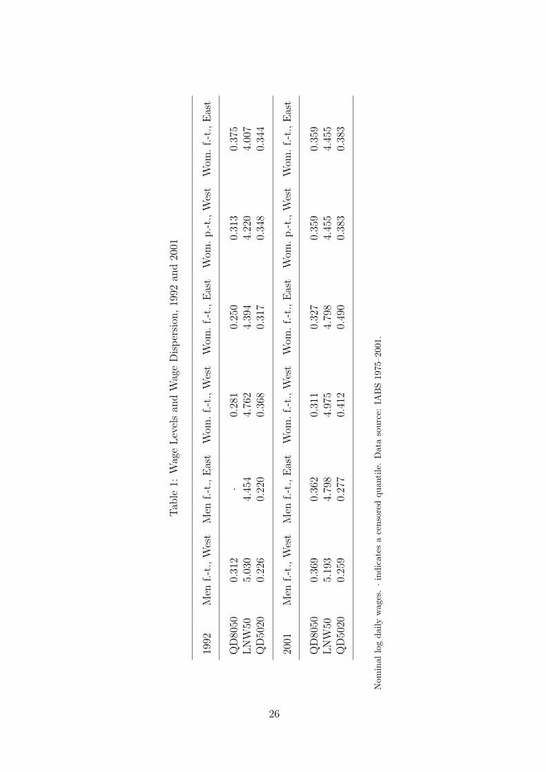
sense to focus on the two boundary years in the following. Table 1 depicts median wages
LNW50 and percentile differences QD8050 and QD5020 for the different groups in 1992
and 2001. As expected, the wage level is generally higher for men compared to women
and for workers in West Germany compared to East Germany in 1992. Until 2001, the
gender wage gap narrowed especially in East Germany. The East-West wage gap in the
wage level also went down, but persisted to some degree for full-time employees. Figure
2 reveals that convergence in—nominal as well as real—wage levels took place until the
year 1996, but then basically stopped: Starting out at 58%, 34%, and 17% in 1992, the
respective nominal differences for men, full-time working women, and part-time working
women all shrunk by 7 to 10 real log percentage points (pp). However, only little variation
is observed from 1996 on. Nominal differences of 38–40% and 18–20% remain for full-time
working men and women, but there is virtually no more difference for part-time working
3At this point I examine nominal wages in order to facilitate East-West comparisons because it is
not clear a priori which price deflator and which base year to choose when comparing East and West
Germany in real terms; see the discussion in Franz and Steiner (2000). When comparing East and West
German wage levels in figure 2 below I also present alternative price normalizations. All comparisons
across time in section 4 are based on real wages, deflated by consumer price indices.
5

women.4
Table 1 further shows that wage dispersion as measured by the percentile differences
generally increased for all groups between 1992 and 2001. With the only exception of
part-time working women the increase was considerably stronger in East Germany than
in West Germany. By the year 2001, the level of wage dispersion in the East even exceeds
the level in the West. Moreover, there are remarkable differences across groups. For
Men in West Germany, QD8050 increased by about 6 pp and QD5020 by 3 pp, adding
up to an increase in the interquintile range QD8020 of 9 pp. The larger part of this
increase therefore is due to changes in the upper part of the distribution.5 Since the
80th percentile for men in East Germany is censored in 1992, an analogous statement
for this group cannot be inferred directly from table 1. Yet the results in section 4 show
that wages for men in East Germany also went up disproportionately in the upper part
of the distribution.6 Having said that, wage inequality among full-time working women
increased disproportionately in the lower half of the distribution, and most strikingly so
in East Germany: whereas QD8050 and QD5020 went up by 3 and 4 pp in the West,
the respective numbers for East Germany are 8 and 17 pp, adding up to a remarkable
increase of the interquintile range QD8020 of 25 pp.
In what follows, the observed distributions are investigated by means of wage regressions
for the years 1992 and 2001 to capture the changes over time. The application of (cen-
sored) quantile regressions allows to look at between and within inequality, and it sets the
stage for the decomposition analyses in section 4. Considering the years 1992 and 2001
is warranted for the following two reasons. First, both years are similar with respect to
their location in the West German business cycle: Whereas the unification boom faded
out in 1992, the year 2001 marked the end of the new economy boom. Second, the labor
force in East Germany dropped sharply from about 10 to below 7 million in the course
of the German unification and most of the immediate downturn took place in 1990 and
1991; see Kommission (1996). Net emigration from East Germany was highest between
1989 and 1991; see Hunt (2006). 1992 was the first year with positive GDP growth in
East Germany after the unification shock (Burda and Hunt, 2001) and thus is the first
year not heavily exposed to distortions resulting from the unification.
4This effect has already been extensively discussed in the literature; see, e. g., Burda and Schmidt
(1997) and Burda and Hunt (2001).5This finding is similar to the trends observed by Fitzenberger (1999) for the period 1975–1990.6The conclusion is also corroborated by Moller’s (2005) result for the core group of medium-skilled
men.
6
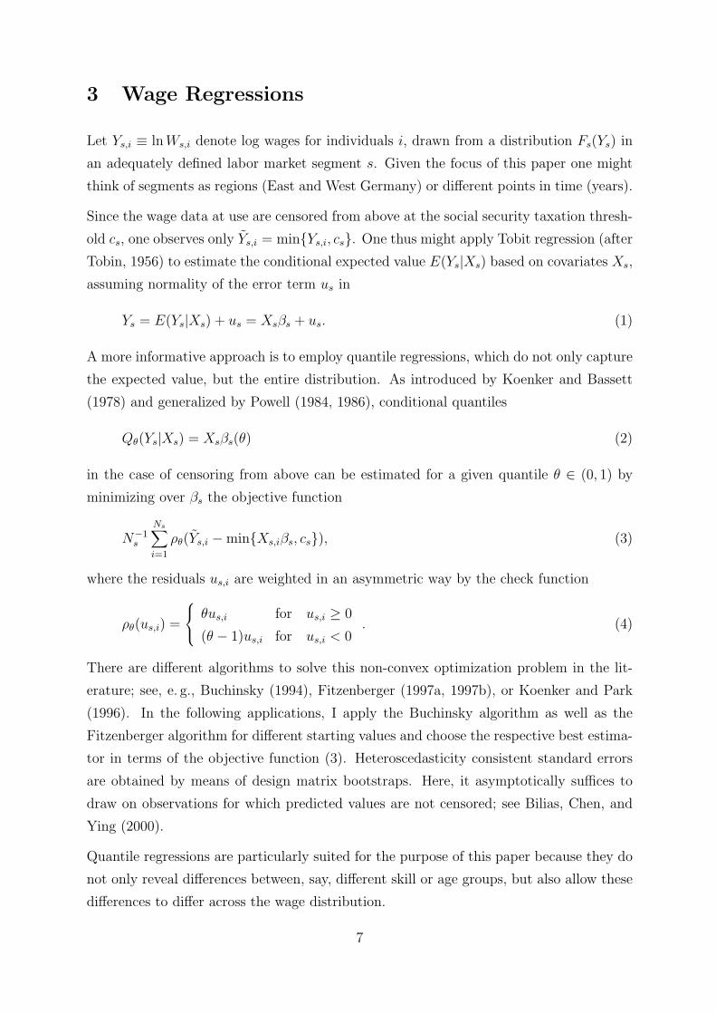
3 Wage Regressions
Let Ys,i ≡ ln Ws,i denote log wages for individuals i, drawn from a distribution Fs(Ys) in
an adequately defined labor market segment s. Given the focus of this paper one might
think of segments as regions (East and West Germany) or different points in time (years).
Since the wage data at use are censored from above at the social security taxation thresh-
old cs, one observes only Ys,i = min{Ys,i, cs}. One thus might apply Tobit regression (after
Tobin, 1956) to estimate the conditional expected value E(Ys|Xs) based on covariates Xs,
assuming normality of the error term us in
Ys = E(Ys|Xs) + us = Xsβs + us. (1)
A more informative approach is to employ quantile regressions, which do not only capture
the expected value, but the entire distribution. As introduced by Koenker and Bassett
(1978) and generalized by Powell (1984, 1986), conditional quantiles
Qθ(Ys|Xs) = Xsβs(θ) (2)
in the case of censoring from above can be estimated for a given quantile θ ∈ (0, 1) by
minimizing over βs the objective function
N−1s
Ns∑
i=1
ρθ(Ys,i −min{Xs,iβs, cs}), (3)
where the residuals us,i are weighted in an asymmetric way by the check function
ρθ(us,i) =
θus,i for us,i ≥ 0
(θ − 1)us,i for us,i < 0. (4)
There are different algorithms to solve this non-convex optimization problem in the lit-
erature; see, e. g., Buchinsky (1994), Fitzenberger (1997a, 1997b), or Koenker and Park
(1996). In the following applications, I apply the Buchinsky algorithm as well as the
Fitzenberger algorithm for different starting values and choose the respective best estima-
tor in terms of the objective function (3). Heteroscedasticity consistent standard errors
are obtained by means of design matrix bootstraps. Here, it asymptotically suffices to
draw on observations for which predicted values are not censored; see Bilias, Chen, and
Ying (2000).
Quantile regressions are particularly suited for the purpose of this paper because they do
not only reveal differences between, say, different skill or age groups, but also allow these
differences to differ across the wage distribution.
7
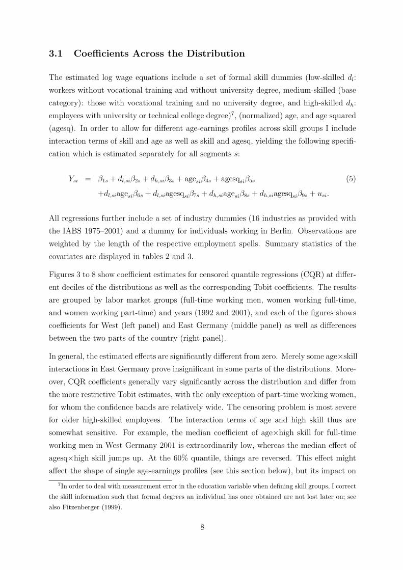
3.1 Coefficients Across the Distribution
The estimated log wage equations include a set of formal skill dummies (low-skilled dl:
workers without vocational training and without university degree, medium-skilled (base
category): those with vocational training and no university degree, and high-skilled dh:
employees with university or technical college degree)7, (normalized) age, and age squared
(agesq). In order to allow for different age-earnings profiles across skill groups I include
interaction terms of skill and age as well as skill and agesq, yielding the following specifi-
cation which is estimated separately for all segments s:
Ysi = β1s + dl,siβ2s + dh,siβ3s + agesiβ4s + agesqsiβ5s (5)
+dl,siagesiβ6s + dl,siagesqsiβ7s + dh,siagesiβ8s + dh,siagesqsiβ9s + usi.
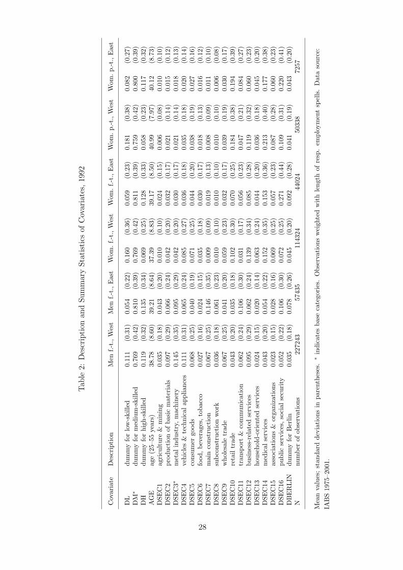
All regressions further include a set of industry dummies (16 industries as provided with
the IABS 1975–2001) and a dummy for individuals working in Berlin. Observations are
weighted by the length of the respective employment spells. Summary statistics of the
covariates are displayed in tables 2 and 3.
Figures 3 to 8 show coefficient estimates for censored quantile regressions (CQR) at differ-
ent deciles of the distributions as well as the corresponding Tobit coefficients. The results
are grouped by labor market groups (full-time working men, women working full-time,
and women working part-time) and years (1992 and 2001), and each of the figures shows
coefficients for West (left panel) and East Germany (middle panel) as well as differences
between the two parts of the country (right panel).
In general, the estimated effects are significantly different from zero. Merely some age×skill
interactions in East Germany prove insignificant in some parts of the distributions. More-
over, CQR coefficients generally vary significantly across the distribution and differ from
the more restrictive Tobit estimates, with the only exception of part-time working women,
for whom the confidence bands are relatively wide. The censoring problem is most severe
for older high-skilled employees. The interaction terms of age and high skill thus are
somewhat sensitive. For example, the median coefficient of age×high skill for full-time
working men in West Germany 2001 is extraordinarily low, whereas the median effect of
agesq×high skill jumps up. At the 60% quantile, things are reversed. This effect might
affect the shape of single age-earnings profiles (see this section below), but its impact on
7In order to deal with measurement error in the education variable when defining skill groups, I correct
the skill information such that formal degrees an individual has once obtained are not lost later on; see
also Fitzenberger (1999).
8

predictions (as used for the decomposition analyses in the next section) can be expected
to be small.
Due to the inclusion of the interaction effects, the interpretation of some of the coefficients
is not apparent, and I resort to looking at age-earnings profiles in the next subsection.
Nevertheless, there are some notable differences of coefficients across quantiles. For exam-
ple, the effect of age is found to become steeper and more concave at higher quantiles for
full-timers. The (negative) base effect of low skill tends to be smallest at low quantiles,
and so does the (positive) base effect of high skill. These results are well in line with the
predictions of human capital theory; see Becker (1993) and Card (1999).
Looking at West-East differences in the coefficients for the year year 1992, differences in
the base effects of skill turn out to be are relatively small. The base trajectory of age is
steeper and slightly more concave for men in West Germany, but the picture is reversed for
full-time working women, most strikingly in the lower half of the distribution. Differences
in the returns to skill among part-time working women are relatively large in the lower
half of the distribution. In the year 2001, the differences in the age effects are basically
the same as in 1992, but now low-skilled men are particularly worse off in East Germany
in the lower half of the distribution. On the other hand, the base return to high skill in
East Germany has increased disproportionately at the upper end of the distribution so
that one finds a negative difference there.
Changes of the coefficients between 1992 and 2001 can be inferred from figures 9 to
14, which rearrange the estimation results in the left two panels and show the changes
between 1992 and 2001 explicitly in the right panel. In West Germany, the base wage
has increased, and for full-timers this effect was stronger at higher quantiles. Base skill
differentials for both men and women (except for high-skilled part-timers at the top of
the distribution) have increased, hinting at an increasing inequality between skill groups.
The base returns to age only changed little, though. The changes in East Germany are
qualitatively comparable to those in the West. Yet the baseline increased even more
distinctly over time, and more pronounced differences across quantiles hint at a higher
degree of within dispersion. The negative base wage premium for low skill has grown most
strikingly at the lower end of the distribution, whereas the base premium for high-skilled
men has grown most at the top of the distribution.
9
3.2 Age-Earnings Profiles
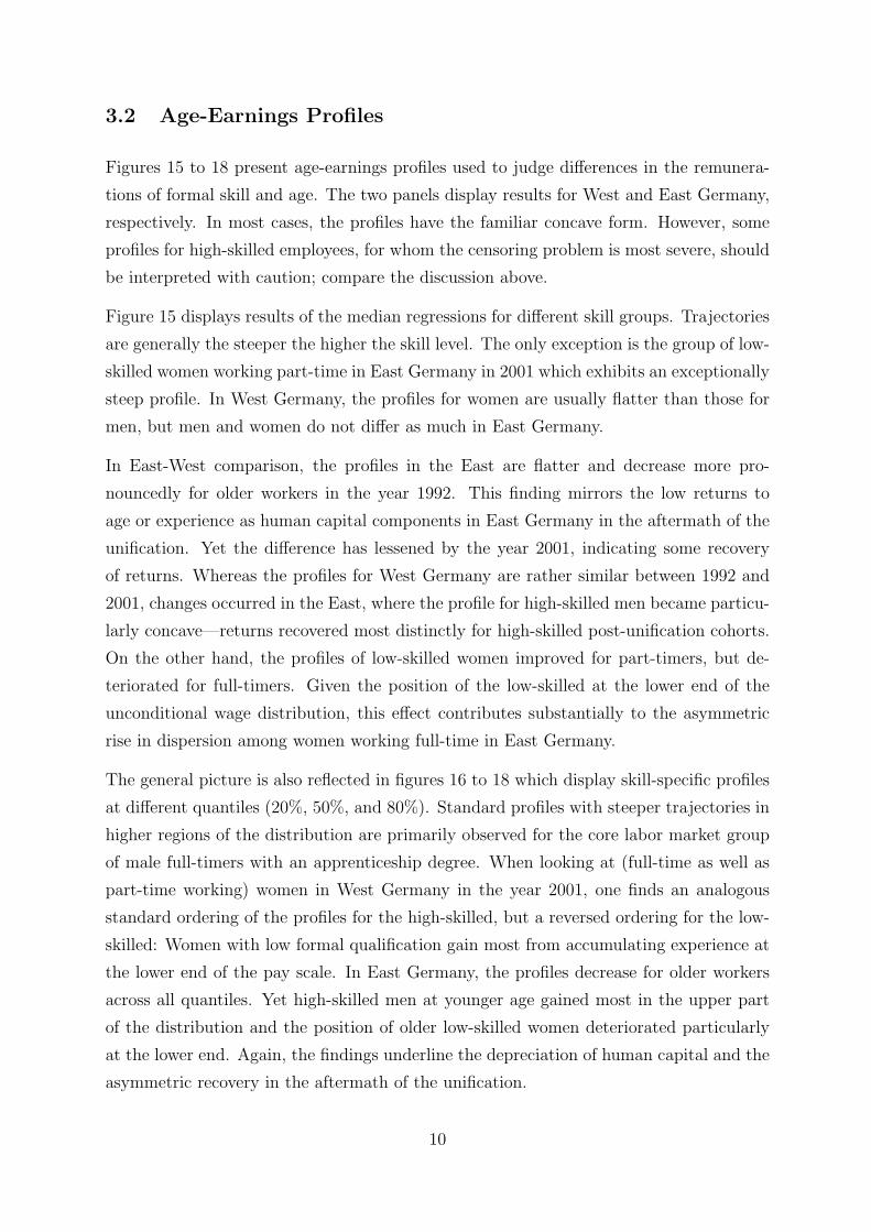
Figures 15 to 18 present age-earnings profiles used to judge differences in the remunera-
tions of formal skill and age. The two panels display results for West and East Germany,
respectively. In most cases, the profiles have the familiar concave form. However, some
profiles for high-skilled employees, for whom the censoring problem is most severe, should
be interpreted with caution; compare the discussion above.
Figure 15 displays results of the median regressions for different skill groups. Trajectories
are generally the steeper the higher the skill level. The only exception is the group of low-
skilled women working part-time in East Germany in 2001 which exhibits an exceptionally
steep profile. In West Germany, the profiles for women are usually flatter than those for
men, but men and women do not differ as much in East Germany.
In East-West comparison, the profiles in the East are flatter and decrease more pro-
nouncedly for older workers in the year 1992. This finding mirrors the low returns to
age or experience as human capital components in East Germany in the aftermath of the
unification. Yet the difference has lessened by the year 2001, indicating some recovery
of returns. Whereas the profiles for West Germany are rather similar between 1992 and
2001, changes occurred in the East, where the profile for high-skilled men became particu-
larly concave—returns recovered most distinctly for high-skilled post-unification cohorts.
On the other hand, the profiles of low-skilled women improved for part-timers, but de-
teriorated for full-timers. Given the position of the low-skilled at the lower end of the
unconditional wage distribution, this effect contributes substantially to the asymmetric
rise in dispersion among women working full-time in East Germany.
The general picture is also reflected in figures 16 to 18 which display skill-specific profiles
at different quantiles (20%, 50%, and 80%). Standard profiles with steeper trajectories in
higher regions of the distribution are primarily observed for the core labor market group
of male full-timers with an apprenticeship degree. When looking at (full-time as well as
part-time working) women in West Germany in the year 2001, one finds an analogous
standard ordering of the profiles for the high-skilled, but a reversed ordering for the low-
skilled: Women with low formal qualification gain most from accumulating experience at
the lower end of the pay scale. In East Germany, the profiles decrease for older workers
across all quantiles. Yet high-skilled men at younger age gained most in the upper part
of the distribution and the position of older low-skilled women deteriorated particularly
at the lower end. Again, the findings underline the depreciation of human capital and the
asymmetric recovery in the aftermath of the unification.
10
4 Decomposing Differences Across Wage Distribu-
tions
The above regression analyses provided detailed insights into the remuneration of observed
worker characteristics in different labor market segments and in different parts of the
wage distribution. Decomposition analyses are well-suited to complement the regression
evidence by answering the question whether differences in observed distributions result
from differences in estimated coefficients or from differences in the composition of the
workforce. I focus on differences between East and West Germany and on changes of the
respective wage structures over time.
A Blinder (1973)-Oaxaca (1973)-type decomposition for the difference between the ex-
pected wages in two segments s and s is:
E(Ys|Xs)− E(Ys|Xs) = (Xs −Xs)βs + Xs(βs − βs). (6)
To apply the Blinder-Oaxaca (B-O) decomposition in case of censored data, I evaluate
equation (6) at mean values of the characteristics and use the coefficients estimated by
means of Tobit regressions.8
The first summand on the right hand side of equation (6), traditionally labelled “char-
acteristics effect”, captures the part of the difference that is attributable to differences
in the covariates across the two segments. The second summand known as “returns” or
“coefficients effect” captures the part of the difference that is attributed to differences
in the returns to the covariates. When decomposing West-East wage gaps in the next
section, I choose the counterfactual XEastβWest to answer the question what the expected
log wage would have been, had a population with the same distribution of characteristics
as East Germany faced returns to characteristics as in the West.9 The approach assumes
that the West German returns are the relevant benchmark for the distribution in the
absence of any “discrimination”. In case of the comparison across time in section 4.2 the
8In contrast to the traditional OLS case, however, the predicted conditional difference does not nec-
essarily coincide with the observed mean difference. “Observed” mean wages in the censoring case have
to be estimated by means of Tobit regressions on a constant.9It is well known that the partition depends on the ordering of the effects and that the decomposition
results may not be invariant with respect to the choice of the involved counterfactual Xsβs; see the surveys
of Oaxaca and Ransom (1994) and Silber and Weber (1999). Therefore, the choice of a counterfactual
should be guided by the question of economic interest.
11
counterfactual X1992β2001 hypothesizes what the expected wage would have been in face of
returns in the year 2001, had the distribution of characteristics not changed since 1992.10
A further method introduced by Juhn, Murphy, and Pierce (1991) and applied in a series
of papers by Blau and Kahn (1992, 1994, 1997) also decomposes the change of a wage gap
over time. This approach has got the additional merit that it decomposes also residual
effects into a quantity and a price effect. However, it suffers from the shortcoming that
it assumes unique coefficients across segments s and s. What is more, the decomposition
of the residual terms is inapplicable in the case of censored data, in which residuals can
only be used for uncensored observations.
The main disadvantage of all techniques discussed so far is that all of them consider only
mean effects. In contrast, Machado and Mata (2005) build on quantile regressions to
decompose differences across entire distributions. They propose an estimator F ∗s (Ys) of
the marginal distribution of wages which conforms to the linear conditional model (2) as
follows:
1. Draw M numbers θ1, ..., θM at random from a uniform distribution U(0, 1).
2. For each θm, estimate the conditional quantile (2), using the sample {Ys,i, Xs,i}Nsi=1.
This yields coefficient estimates βs(θ1), ..., βs(θ
M).
3. Draw M random draws X1s , ..., XM
s from the sample {Xs,i}Nsi=1.
4. Then, the data set {Y ∗ms ≡ Xm
s βs(θm)}M
m=1 constitutes a random sample from
F ∗s (Ys).
An estimator F ∗s (Ys(Xs)) of the counterfactual marginal distribution, which relies on the
coefficients of segment s but on the characteristics of segment s, can be obtained in an
analogous way by drawing resamples from Xs rather than from Xs in the third step.
10There are alternative methodologies to the standard B-O decompositions in the literature. In light
of the present focus on differences in two dimensions, techniques to decompose changes of wage gaps over
time in one single exercise—as proposed by Smith and Welch (1989) or Wellington (1993)—would be of
particular interest. However, I opt to consider both decompositions separately for two reasons. First, any
combination of involved counterfactuals—be it with or without interaction terms between the differences
in characteristics and differences in coefficients—bears an even higher degree of arbitrariness; see Le and
Miller (2004). Second, and most importantly, each of the two comparisons, the differences between East
and West Germany as well as the changes of the wage distributions within the two regions over time, is
interesting of its own.
12
The Machado/Mata (MM) decomposition based on the estimated distributions therefore
writes
Fs(Ys)− Fs(Ys) = F ∗s (Ys)− F ∗
s (Ys) + ε (7)
= [F ∗s (Ys)− F ∗
s (Ys(Xs))] + [F ∗s (Ys(Xs))− F ∗
s (Ys)] + ε,
where Fs(·) denotes an estimator of the distribution based on the observed sample. Similar
to the B-O decomposition, the term in the first brackets on the right hand side of (7)
is a characteristics effect, and the one in the second brackets a returns effect. Provided
that the linear specification (2) is appropriate, the residual term ε is negligible for large
samples. With respect to the choice of a counterfactual distribution the same caveat as
in the B-O case applies.
I employ the MM technique, resorting to quantile measures for the involved distributions
in order to gauge the elements of the decompositions. However, a couple of adaptations
are undertaken. First, I estimate CQR as explained above. Second, I follow Albrecht,
Bjorklund, and Vroman (2001) to save computation time: Rather than drawing M random
numbers for θm and then estimating M (censored) quantile regressions, I estimate one
regression for each single percentile and then draw M = 1000 random draws from the
distributions of the covariates for each βs(·). Third, and finally, predictions above the
SSTT are censored to this value in order to replicate the censoring of the wage data.
As a consequence, all comparisons of the simulated distributions F ∗s (·) consider only the
respective uncensored parts.
There are also alternative approaches in the literature for decomposing differences across
entire distributions. The decomposition introduced by Juhn, Murphy, and Pierce (JMP,
1993), which is also used by Blau and Kahn (1996) for cross-country comparisons and
by Steiner and Wagner (1997, 1998) and Gernandt and Pfeiffer (2006) for German data,
employs the distribution of residuals resulting from wage regressions to rank observations.
This approach gives a structural interpretation to the regression residual. Yet it faces
a couple of shortcomings. First, its focus on the distribution of residuals renders the
approach as inapplicable in the case of censored data as the related (1991) approach.
Second, even without censoring of the data, the JMP (1993) decomposition is valid only
in the case of homoscedasticity, which is usually rejected for empirical wage regressions.
Third, and most importantly, it is more restrictive than the MM technique because it
assumes a single linear model to hold for the entire wage distribution, whereas the latter
approach based on quantile regressions allows for flexibility across the distribution.
13

Autor, Katz, and Kearney (2005a) also build on the MM approach, while DiNardo, Fortin,
and Lemieux (1996) exploit kernel density estimations to decompose differences in a non-
parametric setting. Compared to this approach, the semiparametric MM framework is
restrictive by nature. Yet by quantifying differences in the coefficients it sheds light on
that part of a difference which would be left unexplained in the nonparametric framework.
4.1 Differences between East and West Germany
Table 4 reports observed and predicted West-East differences in log wages across quantiles
for the years 1992 and 2001.11 Observed and predicted quantiles of the unconditional
wage distributions show a close resemblance, therefore suggesting that the estimation and
specification error is of minor importance. The predicted gaps thus broaden the snapshot
discussion of section 2. Decile differences which cannot be interpreted due to the censoring
problem are marked by a dot. The Tobit results reported in the last column are usually
close to the values at the median.
For the group of full-time working men the gap varies between 55% at the first decile
and 61% at the eighth decile in 1992. The observation that the gap at the upper end
of the distribution exceeds the gap at the lower end by 6 pp indicates a higher wage
dispersion in the West as compared to the East. In 2001 the East-West differential varies
less between quantiles (38% at the first decile and 40% at the eighth): Wage dispersion in
East Germany has caught up to a large degree. Except for the difference in the level, the
picture for women working full-time in 1992 is very similar to that for males in the upper
two thirds of the distribution: The gaps at the third and at the eighth decile differ by 4
pp. However, the gap of 22% at the first decile falls below the gap at the third decile by
remarkable 14 pp—at the very low end of the distribution the West-East gap is less severe.
This finding still holds for the year 2001, but now the differential at the third decile also
exceeds the differential at the eighth by 9 pp: The upper half of this group’s distribution
participated most strikingly in the closing of the West-East wage gap. Women working
part-time in East Germany in 1992 were relatively well off at the low and at the high
end of the distribution, and the West-East differential was highest around the median.
The differential for this group had basically vanished by 2001, though. At the first decile
wages were even slightly higher in the East.
When decomposing West-East wage differentials in order to judge whether the differentials
stem from different decompositions of the work force or whether employees’ characteristics
11The analysis in this section is based on nominal numbers; see the discussion in section 2.
14
are remunerated differently in East and West Germany, one generally finds relatively
small impacts of the characteristics. The better parts of the differentials are in most cases
captured by differences in the coefficients.
For full-time working men the characteristics effect is largely negligible in both years 1992
and 2001. If anything, different characteristics explain 2 pp of the West-East differential
in the upper part of the distribution in 2001. In the group of women working full-time in
1992, the characteristics effect ranges between –9 pp at the first decile and –6 pp at the
eighth. It therefore is in favor of higher earnings in East Germany and most pronounced
in the lower half of the distribution. In relative terms, women selecting into full-time
jobs in East Germany had more preferable characteristics in 1992. This tendency still
holds for 2001, but to a lesser degree and mainly in the upper half of the distribution. In
the lower part of the distribution the relative deterioration of characteristics contributed
substantially to the worsened position in the pay scale. A similar reasoning also applies for
women working part-time in 1992. However, there are only little offsetting characteristics
and coefficients effects in the year 2001, by which convergence of wages has been achieved
for this group.
The conclusion that differences in employees’ characteristics only play a minor role in
explaining East-West wage differentials is supported by the summary statistics of the
covariates in tables 2 and 3. By and large, differences are very small. In both years 1992
and 2001 and for all labor market groups, the level of formal education in East Germany
is higher than in the West. Only the proportion of male employees with a university
degree is higher in West Germany in 2001.
The latter finding is in line with the results of the B-O decompositions in Burda and
Schmidt (1997) and the JMP decompositions in Steiner and Wagner (1997), both of
which use GSOEP data for the early 1990s and report a minor importance of differences
in the characteristics of the work forces. Gorzig, Gornig, and Werwatz (2004), using
a decomposition based on establishment-level data, compare wages in East and West
Germany for the years 1994 and 1998. They stress the importance of differences in
establishment types and conclude that the catching-up in the East was in part offset by
an increasing share of low-wage-type establishments in East Germany. The analysis of
East-West migrants in Kirbach and Smolny (2004) also concludes that only a small part of
observed East-West wage gaps can be attributed to observed socioeconomic characteristics
of the workers.
15
4.2 Changes in the Wage Structure Over Time
In order to analyze changes in the wage structure over time, I use real wages (normalized
by consumer prices of 1992, differentiated by regions). In a setup analogous to that of
table 4 in the previous section, the panels in table 5 display the observed and predicted
log wage changes between 1992 and 2001. Differences of the numbers across quantiles
give account of the evolution of wage inequality.
Among the group of men working full-time in West Germany, inequality as measured by
percentile differences QD8020 has increased by 9 pp and this increase was slightly more
pronounced in the upper half of the distribution. The eighth decile gained 5% while the
second decile lost by 4%. Due to the censoring problem, changes at the very high end of
the distribution cannot be assessed, but wages at the very low end exhibited a remarkable
real loss of almost 8%. The (predicted) interquintile range QD8020 of 14 pp for men
in East Germany shows that wage dispersion went up even more remarkably. Moreover,
most of this increase (10 pp) took place in the upper half of the distribution. Yet even at
the lower end real wage growth was positive for this group.
Real wages of women working full-time in West Germany did hardly change in the lower
third of the distribution. Only the first decile exhibited a decline of 2%. Negative real
wage growth of up to –4% is found in the lower third of the distribution for this group
in East Germany. The gender wage gap in East Germany thus did not close, but rather
widen in this part of the distribution. Wage growth further differed substantially at higher
quantiles: Whereas Western wages increased by up to 8%, wages in the East went up by
remarkable 23% at the eighth decile. The corresponding interquintile range QD8020 of
25 pp shows that the increase in inequality was most striking among this group.
The group of part-time working women in West Germany experienced real wage growth
between 5 and 11%, with highest increases at the extreme deciles. In East Germany, the
range of differences across quantiles is 9 pp. However, the biggest increase is observed
in the middle part of the distribution and—well in line with the observed closing of the
East-West gap for this group—the level of changes exceeds that in the West by about 10
pp.
The decomposition of the wage changes reveals characteristics effects in the range between
1 pp (in favor of higher earnings in 2001) at the first decile and 5 pp at the eighth decile for
all three labor market groups working in West Germany. With shares of about one half for
women and virtually full coverage for men, changes in the characteristics therefore capture
the better part of the respective wage increases in the upper halves of the distributions.
16
The finding likely reflects some skill upgrading in the prime-age work force. In fact,
reconsidering the summary statistics of the covariates in tables 2 and 3, one finds that
skill upgrading took place in both East and West Germany between 1992 and 2001. As
the proportion of low-skilled workers decreased in all labor market groups, the proportion
of high-skilled went up. This increase was more pronounced in West Germany than in the
East. With respect to changes in the industry structure of the work force, employment in
public and social security system services (sector 16) decreased most remarkably in East
Germany.
Restructuring and skill upgrading yet played only a minor role in explaining the strik-
ing wage increase (especially in the upper half of the distribution) for men working in
East Germany: The characteristics effect does not exceed 2 pp. A similar result holds
for the majority of women working full-time in East Germany, but for this group the
characteristics effect goes down up to –7 pp in the lower middle of the distribution. The
characteristics in that part of the distribution working toward real wage cuts, the increas-
ing inequality was driven by a more advantageous development of characteristics at the
upper end. Finally, the contribution of changes in the characteristics is largely negligi-
ble across the entire distribution of wage changes for women working part-time in East
Germany.
A bottom line of this exercise is that the diverse patterns of changing wage levels and
increasing inequality are due to changes in the composition of the respective work forces
and changing remunerations of relevant characteristics. This result differs from that of
related studies in the literature12, all of which use the more restrictive B-O or JMP
decompositions for different periods of time and find basically no composition effects
among prime-age employees.
5 Conclusions
The German wage structure has been rather compressed in international comparison
and “unbearabl[y] stable” (Prasad, 2000) between the mid 1970s and the mid-1990s.
Newly available register data from the IAB employment sample 1975–2001 now allow
12Steiner and Wagner (1998) analyze the evolution of wage inequality among West German males by
means of JMP decompositions applied to GSOEP and IABS data for the years 1984–1990. Note that
their analysis for the IABS bears some problems because it only considers uncensored wages. Burda and
Hunt (2001) apply B-O decompositions to the GSOEP East 1990–1999. Gernandt and Pfeiffer (2006)
also use GSOEP data for 1984–2004 and apply JMP decompositions.
17
to reinvestigate the empirical evidence for more recent years. This paper studies the
evolution of wage levels and wage inequality within and between different labor market
groups for the years 1992–2001. I find that wage inequality has in fact been rising in
many dimensions throughout this period.
A comparison of mean wage differences reveals that convergence in wage levels between
West and East Germany took place up to the year 1996, but nominal differences of about
40% for men and 20% for full-time working women persisted until 2001. No more difference
is observed in the wages of part-time working women.
The inspection of year-specific wage distributions unveils rising wage dispersion. As mea-
sured by interquintile ranges QD8020, dispersion was generally lower in East Germany
than in West Germany in the year 1992, but it caught up until 2001: Whereas QD8020
increased by 8 to 9 log percentage points (pp) for men and full-time working women in
West Germany, the corresponding numbers are 14 to 25 pp in the East. Moreover, the
larger part of the increase in dispersion among women happened in the lower parts of the
respective distributions, but dispersion among men increased disproportionately in the
upper parts.
The estimation of censored quantile wage regressions provides insights into the determi-
nants of the observed differences and changes. The bottom line of the regression results
meets a-priori expectations. Age-earnings profiles not only are the steeper the higher the
skill level, but they are also relatively flat in East Germany in 1992. The unification
shock clearly led to a depreciation of human capital in the East. However, this effect
wears out with the aging of post-unification labor market cohorts, and differences in the
profiles between East and West Germany have lessened by the year 2001. The quantile
regression approach further reveals significant differences in the effects across the wage
distribution. The result that low-skilled women working full-time in East Germany are
left particularly worse-off at the lower end of the distribution substantiates the high and
asymmetric increase in dispersion for this group.
Drawing on the flexible quantile regression approach, the decomposition technique intro-
duced by Machado and Mata (2005) is well-suited to depict heterogeneous characteristics
and coefficients effects across the respective wage distributions. In East-West compari-
son, differences in the composition of the work force turn out largely negligible for men.
However, characteristics of full-time working women are mostly in favor of higher wages
in the East. Yet this effect ceased to apply at the lower end of the distribution by the
year 2001.
18

With respect to the evolution of wages over time, characteristics effects capture major
parts of the respective wage increases in the upper halves of the wage distributions for
West Germany. This finding reflects a skill upgrading in the work force. Restructuring
and skill upgrading yet played only a minor role in explaining the wage increases in East
Germany. For women in the lower parts of the Eastern distribution the characteristics
effect even worked toward real wage cuts, substantiating again the particular increase in
wage dispersion among this group.
The finding of rising wage inequality is broadly in line with the evidence in Moller (2005),
who compares decile ratios for selective labor market groups and also stresses the impor-
tance to distinguish between men and women when assessing asymmetries in the evolution
of wage inequality. Gernandt and Pfeiffer (2006), also reporting increasing wage inequal-
ity, do not distinguish between sexes and therefore do not give account of the striking
asymmetries between the groups in East Germany. As a consequence, their JMP decom-
positions do not detect this effect, either.
All of the results discussed in this paper are descriptive by nature. Unfortunately, the
IABS provides only relatively few covariates, such that it is impossible to venture upon
instrumental variable estimation or a control function approach in order to account for a
possible endogeneity of educational attainment or differences in the selection into the labor
market. The analysis focusses on core labor market groups and leaves aside marginal part-
time workers (geringfugig Beschaftigte), among others. This is important to note because
it renders the finding of increasing inequality even more meaningful.
An analogous argument applies with respect to migration, which is not modeled explicitly.
East-West migration in the aftermath of the unification had already come down to stable
numbers by the year 1992 and the evidence for the existence of a brain drain is mixed; see
Arntz (2006), Buchel, Frick, and Witte (2002), and Hunt (2006). However, if emigration
from East Germany during the observation period is skill- or age-biased, i. e., if migrants
are in fact either better educated workers or low-skilled who have been laid-off (Hunt,
2006), the observation that wage inequality increases faster in East Germany is even
more remarkable.
Finally, it is not the aim of this paper to speculate about the economic causes and con-
sequences of the unveiled trends. In face of alternative explanatory hypotheses—such as
accelerating non-neutral technical change, increasingly heterogenous work environments,
more flexible labor market institutions, or a decline in union power—estimates of struc-
tural models may be expected to complement the descriptive evidence in future research.
19

References
Acemoglu, D. (2002): “Technical Change, Inequality, and the Labor Market,” Journal
of Economic Literature, 40, 7–72.
Albrecht, J., A. Bjorklund, and S. Vroman (2001): “Is There a Glass Ceiling in
Sweden?,” Journal of Labor Economics, 21(1), 145–177.
Arntz, M. (2006): “What attracts human capital? Understanding the skill composition
of internal migration flows in Germany,” unpublished manuscript, ZEW Mannheim.
Autor, D. H., L. F. Katz, and M. S. Kearney (2005a): “Rising Wage Inequality:
The Role of Composition and Prices,” Working Paper 11628, NBER.
(2005b): “Trends in U.S. Wage Inequality: Re-Assessing the Revisionists,”
Working Paper 11627, NBER.
Buchel, F., J. R. Frick, and J. C. Witte (2002): “Regionale und berufliche Mo-
bilitat von Hochqualifizierten – Ein Vergleich Deutschland–USA,” in Arbeitsmarkte
fur Hochqualifizierte, ed. by L. Bellmann, and J. Velling, Beitrage zur Arbeitsmarkt-
und Berufsforschung 256, pp. 207–243. Institut fur Arbeitsmarkt- und Berufsforschung,
Nurnberg.
Becker, G. S. (1993): Human Capital: A Theoretical and Empirical Analysis with
Special Reference to Education. The University of Chicago Press, Chicago, London, 3rd
edn.
Bender, S., A. Haas, and C. Klose (2000): “The IAB Employment Subsample
1975–1995,” Schmollers Jahrbuch, 120(4), 649–662.
Bender, S., J. Hilzendegen, G. Rohwer, and H. Rudolph (1996): Die IAB-
Beschaftigtenstichprobe 1975–1990, Beitrage zur Arbeitsmarkt- und Berufsforschung
197. Institut fur Arbeitsmarkt- und Berufsforschung, Nurnberg.
Bilias, Y., S. Chen, and Z. Ying (2000): “Simple Resampling Methods for Censored
Regression Quantiles,” Journal of Econometrics, 99, 373–386.
Bird, E. J., J. Schwarze, and G. Wagner (1994): “Wage Effects of the Move
Toward Free Markets in East Germany,” Industrial and Labor Relations Review, 47(3),
390–400.
20
Blau, F. D., and L. M. Kahn (1992): “The Gender Earning Gap: Learning from In-
ternational Comparisons,” American Economic Review, 82(2, Papers and Proceedings),
533–538.
(1994): “Rising Wage Inequality and the U.S. Gender Gap,” American Economic
Review, 84(2, Papers and Proceedings), 23–28.
(1996): “International Differences in Male Wage Inequality: Institutions versus
Market Forces,” Journal of Political Economy, 104(4), 791–837.
(1997): “Swimming Upstream: Trends in the Gender Wage Differential in the
1980s,” Journal of Labor Economics, 15(1), 1–42.
Blinder, A. S. (1973): “Wage Discrimination: Reduced Form and Structural Esti-
mates,” Journal of Human Resources, 8(4), 436–455.
Buchinsky, M. (1994): “Changes in the U.S. Wage Structure 1963–1987: Application
of Quantile Regression,” Econometrica, 62(2), 405–458.
Burda, M. C., and J. Hunt (2001): “From Reunification to Economic Integration:
Productivity and the Labor Market in Eastern Germany,” Brookings Papers on Eco-
nomic Activity, 2, 1–92, including discussions.
Burda, M. C., and C. M. Schmidt (1997): “Getting behind the East-West Wage
Differential: Theory and Evidence,” in Wandeln oder Weichen – Herausforderungen
der wirtschaftlichen Integration fur Deutschland, ed. by R. Pohl, and H. Schneider, pp.
170–201. IWH Halle, Sonderheft Wirtschaft im Wandel.
Card, D. (1999): “The Causal Effect of Education on Earnings,” in Handbook of Labor
Economics, ed. by O. Ashenfelter, and D. Card, vol. 3, chap. 30, pp. 1801–1863. Elsevier
Science.
DiNardo, J., N. M. Fortin, and T. Lemieux (1996): “Labor Market Institutions and
the Distribution of Wages, 1973–1992: A Semiparametric Approach,” Econometrica,
64(5), 1001–1044.
Fitzenberger, B. (1997a): “A Guide to Censored Quantile Regressions,” in Handbook
of Statistics, ed. by G. S. Maddala, and C. R. Rao, vol. 15: Robust Inference, pp.
405–437. Elsevier Science.
21

(1997b): “Computational aspects of censored quantile regression,” in L1-
Statistical Procedures and Related Topics, ed. by Y. Dodge, vol. 31 of IMS Lecture Notes
– Monograph Series, pp. 171–186. Institute of Mathematical Statistics, Hayward, CA.
(1999): Wages and Employment Across Skill Groups: An Analysis for West
Germany. Physica, Heidelberg.
Fitzenberger, B., and K. Kohn (2005): “Skill Wage Premia, Employment, and Co-
hort Effects in a Model of German Labor Demand,” unpublished manuscript, Goethe-
University Frankfurt.
Franz, W., and V. Steiner (2000): “Wages in the East German Transition Process:
Facts and Explanations,” German Economic Review, 1(3), 241–269.
Gernandt, J., and F. Pfeiffer (2006): “Rising Wage Inequality in Germany,” Dis-
cussion Paper 06-19, ZEW Mannheim.
Gorzig, B., M. Gornig, and A. Werwatz (2004): “East Germanys Wage Gap:
A non-parametric decomposition based on establishment characteristics,” Discussion
Paper 451, DIW Berlin.
Hamann, S., G. Krug, M. Kohler, W. Ludwig-Mayerhofer, and A. Hacket
(2004): “Die IAB-Regionalstichprobe 1975–2001: IABS-R01,” ZA-Information, 55, 34–
59.
Hunt, J. (2001): “Post-Unification Wage Growth in East Germany,” Review of Eco-
nomics and Statistics, 83(1), 190–195.
(2006): “Staunching Emigration from East Germany: Age and the Determinants
of Migration,” Journal of the European Economic Association, p. forthcoming.
Juhn, C., K. M. Murphy, and B. Pierce (1991): “Accounting for the slowdone in
black-white wage convergence,” in Workers and their Wages, ed. by M. H. Kosters, pp.
107–143. AEI Press.
(1993): “Wage Inequality and the Rise in Returns to Skill,” Journal of Political
Economy, 101(3), 410–442.
Katz, L. F., and D. H. Autor (1999): “Changes in the Wage Structure and Earnings
Inequality,” in Handbook of Labor Economics, ed. by O. Ashenfelter, and D. Card,
vol. 3, chap. 26, pp. 1463–1555. Elsevier Science.
22
Kirbach, M., and W. Smolny (2004): “Wage differentials between East and West
Germany – Is it related to the location or to the people?,” unpublished manuscript,
University of Ulm and ZEW, Mannheim.
Koenker, R., and G. Bassett, Jr. (1978): “Regression Quantiles,” Econometrica,
46(1), 33–50.
Koenker, R., and B. J. Park (1996): “An interior point algorithm for nonlinear
quantile regression,” Journal of Econometrics, 71, 265–283.
Kommission fur Zukunftsfragen der Freistaaten Bay-
ern und Sachsen (1996): “Erwerbstatigkeit und Arbeitslosigkeit
in Deutschland – Entwicklung, Ursachen und Maßnahmen,”
http://www.bayern.de/imperia/md/content/stk/allgemein/bericht1.pdf.
Krueger, A., and J.-S. Pischke (1995): “A Comparative Analysis of East and West
German Labor Markets: Before and After Unification,” in Differences and Changes in
Wage Structures, ed. by R. B. Freeman, and L. F. Katz, pp. 405–445. University of
Chicago Press, Chicago, London.
Le, A. T., and P. W. Miller (2004): “Inter-Temporal Decompositions of Labour
Market and Social Outcomes,” Australian Economic Papers, 43(1), 10–20.
Machado, J. A. F., and J. Mata (2005): “Counterfactual Decomposition of Changes
in Wage Distributions using Quantile Regression,” Journal of Applied Econometrics,
20(4), 445–465.
Moller, J. (2005): “Die Entwicklung der Lohnspreizung in West- und Ostdeutschland,”
in Institutionen, Lohne und Beschaftigung, ed. by L. Bellmann, O. Hubler, W. Meyer,
and G. Stephan, Beitrage zur Arbeitsmarkt- und Berufsforschung 294, pp. 47–63. In-
stitut fur Arbeitsmarkt- und Berufsforschung, Nurnberg.
Oaxaca, R. (1973): “Male-female wage differentials in urban labour markets,” Interna-
tional Economic Review, 14, 693–709.
Oaxaca, R. L., and M. R. Ransom (1994): “On discrimination and the decomposition
of wage differentials,” Journal of Econometrics, 61, 5–21.
Powell, J. L. (1984): “Least absolute deviations for the censored regression model,”
Journal of Econometrics, 25, 303–325.
(1986): “Censored regression quantiles,” Journal of Econometrics, 32, 143–155.
23
Prasad, E. S. (2000): “The Unbearable Stability of the German Wage Structure: Evi-
dence and Interpretation,” Working Paper 00/22, IMF.
Riphahn, R. (2003): “Bruttoeinkommensverteilung in Deutschland 1984–1999 und Un-
gleichheit unter auslandischen Erwerbstatigen,” in Wechselwirkungen zwischen Arbeits-
markt und sozialer Sicherung II, ed. by W. Schmahl, vol. 294 of Schriften des Vereins
fur Socialpolitik, pp. 135–174. Duncker & Humblot, Berlin.
Schwarze, J. (1993): “Qualifikation, Uberqualifikation und Phasen des Transforma-
tionsprozesses – Die Entwicklung der Lohnstruktur in den neuen Bundeslandern,”
Jahrbucher fur Nationalokonomie und Statistik, 211, 90–107.
Schwarze, J., and G. Wagner (1992): “Lohnstruktur und Lohnniveau in den neuen
Bundeslandern,” Wirtschaftsdienst, pp. 202–206, Heft IV.
Silber, J., and M. Weber (1999): “Labour market discrimination: are there significant
differences between the various decomposition procedures?,” Applied Economics, 31,
359–356.
Smith, J. P., and F. R. Welch (1989): “Black Economic Progress After Myrdal,”
Journal of Economic Literature, 27, 519–564.
Steiner, V., and T. Holzle (2000): “The Development of Wages in Germany in the
1990s – Description and Explanations,” in The Personal Distribution of Income in an
International Perspective, ed. by R. Hauser, and I. Becker, pp. 7–30. Springer.
Steiner, V., and K. Wagner (1997): “East-West Wage Convergence – How Far Have
We Got?,” Discussion Paper 97-25, ZEW Mannheim.
(1998): “Has Earnings Inequality in Germany Changed in the 1980’s?,”
Zeitschrift fur Wirtschafts- und Sozialwissenschaften, 118(1), 29–59.
Tobin, J. (1956): “Estimation of Relationships for Limited Dependent Variables,”
Econometrica, 26, 24–36.
Wellington, A. J. (1993): “Changes in the Male/Female Wage Gap, 1976–85,” Journal
of Human Resources, 28(2), 383–411.
24
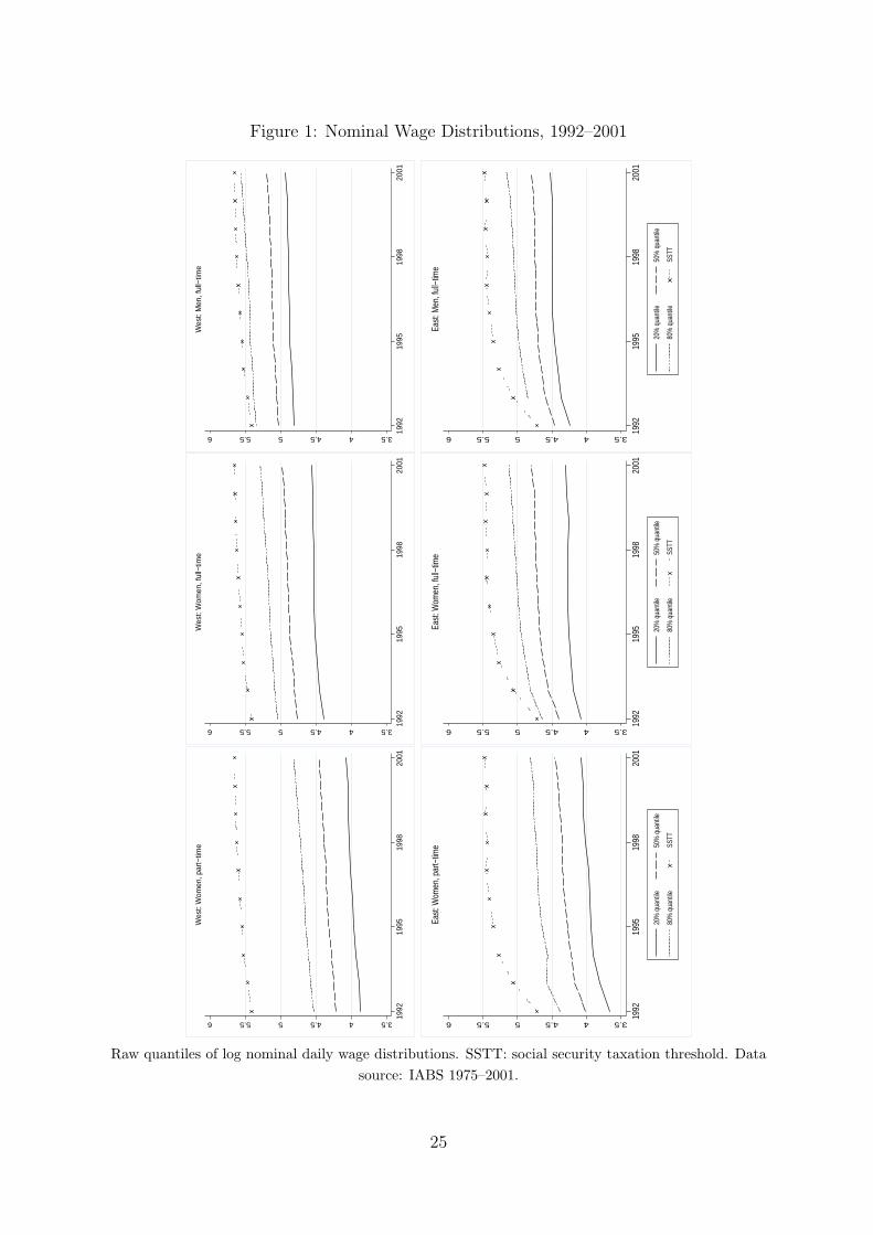
Figure 1: Nominal Wage Distributions, 1992–2001
3.544.555.56 1992
1995
1998
2001
Wes
t: M
en, f
ull−
time
3.544.555.56 1992
1995
1998
2001
20%
qua
ntile
50%
qua
ntile
80%
qua
ntile
SSTT
East
: Men
, ful
l−tim
e
3.544.555.56 1992
1995
1998
2001
Wes
t: W
omen
, ful
l−tim
e
3.544.555.56 1992
1995
1998
2001
20%
qua
ntile
50%
qua
ntile
80%
qua
ntile
SSTT
East
: Wom
en, f
ull−
time
3.544.555.56 1992
1995
1998
2001
Wes
t: W
omen
, par
t−tim
e3.544.555.56 19
9219
9519
9820
01
20%
qua
ntile
50%
qua
ntile
80%
qua
ntile
SSTT
East
: Wom
en, p
art−
time
Raw quantiles of log nominal daily wage distributions. SSTT: social security taxation threshold. Datasource: IABS 1975–2001.
25
Tab
le1:
Wag
eLev
els
and
Wag
eD
isper
sion
,19
92an
d20
01
1992
Men
f.-t
.,W
est
Men
f.-t
.,E
ast
Wom
.f.-t
.,W
est
Wom
.f.-t
.,E
ast
Wom
.p.-t.
,W
est
Wom
.f.-t
.,E
ast
QD
8050
0.31
2·
0.28
10.
250
0.31
30.
375
LN
W50
5.03
04.
454
4.76
24.
394
4.22
04.
007
QD
5020
0.22
60.
220
0.36
80.
317
0.34
80.
344
2001
Men
f.-t
.,W
est
Men
f.-t
.,E
ast
Wom
.f.-t
.,W
est
Wom
.f.-t
.,E
ast
Wom
.p.-t.
,W
est
Wom
.f.-t
.,E
ast
QD
8050
0.36
90.
362
0.31
10.
327
0.35
90.
359
LN
W50
5.19
34.
798
4.97
54.
798
4.45
54.
455
QD
5020
0.25
90.
277
0.41
20.
490
0.38
30.
383
Nom
inal
log
daily
wag
es.·i
ndic
ates
ace
nsor
edqu
anti
le.
Dat
aso
urce
:IA
BS
1975
–200
1.
26

Figure 2: West-East Wage Gaps, 1992–2001
.35
.4.4
5.5
.55
.6
1992 1995 1998 2001
Men, full−time
.15
.2.2
5.3
.35
1992 1995 1998 2001
Women, full−time
0.0
5.1
.15
.2
1992 1995 1998 2001
nominal real, P1992 = 1 real, P2001 = 1
Women, part−time
Differences of mean log wages, estimated by Tobit regressions on a constant. Data source: IABS1975–2001.
27
Tab
le2:
Des
crip
tion
and
Sum
mar
ySta
tist
ics
ofC
ovar
iate
s,19
92
Cov
aria
teD
escr
ipti
onM
enf.-
t.,W
est
Men
f.-t.
,E
ast
Wom
.f.-
t.,W
est
Wom
.f.-
t.,E
ast
Wom
.p.
-t.,
Wes
tW
om.p.
-t.,
Eas
t
DL
dum
my
for
low
-ski
lled
0.11
1(0
.31)
0.05
4(0
.22)
0.16
0(0
.36)
0.05
9(0
.23)
0.18
1(0
.38)
0.08
2(0
.27)
DM∗
dum
my
for
med
ium
-ski
lled
0.76
9(0
.42)
0.81
0(0
.39)
0.76
9(0
.42)
0.81
1(0
.39)
0.75
9(0
.42)
0.80
0(0
.39)
DH
dum
my
for
high
-ski
lled
0.11
9(0
.32)
0.13
5(0
.34)
0.06
9(0
.25)
0.12
8(0
.33)
0.05
8(0
.23)
0.11
7(0
.32)
AG
Eag
e(2
5–55
year
s)38
.78
(8.6
0)39
.21
(8.6
4)37
.39
(8.8
3)39
.17
(8.5
0)40
.99
(7.9
7)40
.12
(8.7
3)D
SEC
1ag
ricu
ltur
e&
min
ing
0.03
5(0
.18)
0.04
3(0
.20)
0.01
0(0
.10)
0.02
4(0
.15)
0.00
6(0
.08)
0.01
0(0
.10)
DSE
C2
prod
ucti
onof
basi
cm
ater
ials
0.09
7(0
.29)
0.06
6(0
.24)
0.04
2(0
.20)
0.03
2(0
.17)
0.02
1(0
.14)
0.01
5(0
.12)
DSE
C3∗
met
alin
dust
ry,m
achi
nery
0.14
5(0
.35)
0.09
5(0
.29)
0.04
2(0
.20)
0.03
0(0
.17)
0.02
1(0
.14)
0.01
8(0
.13)
DSE
C4
vehi
cles
&te
chni
calap
plia
nces
0.11
1(0
.31)
0.06
5(0
.24)
0.08
5(0
.27)
0.03
6(0
.18)
0.03
5(0
.18)
0.02
0(0
.14)
DSE
C5
cons
umer
good
s0.
068
(0.2
5)0.
040
(0.1
9)0.
071
(0.2
5)0.
044
(0.2
0)0.
038
(0.1
9)0.
027
(0.1
6)D
SEC
6fo
od,be
vera
ges,
toba
cco
0.02
7(0
.16)
0.02
4(0
.15)
0.03
5(0
.18)
0.03
0(0
.17)
0.01
8(0
.13)
0.01
6(0
.12)
DSE
C7
mai
nco
nstr
ucti
on0.
067
(0.2
5)0.
146
(0.3
5)0.
009
(0.0
9)0.
019
(0.1
3)0.
008
(0.0
9)0.
011
(0.1
0)D
SEC
8su
bcon
stru
ctio
nw
ork
0.03
6(0
.18)
0.06
1(0
.23)
0.01
0(0
.10)
0.01
0(0
.10)
0.01
0(0
.10)
0.00
6(0
.08)
DSE
C9
who
lesa
letr
ade
0.06
7(0
.25)
0.04
1(0
.20)
0.05
9(0
.23)
0.03
2(0
.17)
0.03
9(0
.19)
0.03
0(0
.17)
DSE
C10
reta
iltr
ade
0.04
3(0
.20)
0.03
5(0
.18)
0.10
2(0
.30)
0.07
0(0
.25)
0.18
4(0
.38)
0.19
4(0
.39)
DSE
C11
tran
spor
t&
com
mun
icat
ion
0.06
2(0
.24)
0.10
6(0
.30)
0.03
1(0
.17)
0.05
6(0
.23)
0.04
7(0
.21)
0.08
4(0
.27)
DSE
C12
busi
ness
-rel
ated
serv
ices
0.09
5(0
.29)
0.06
2(0
.24)
0.13
9(0
.34)
0.08
5(0
.28)
0.11
9(0
.32)
0.06
0(0
.23)
DSE
C13
hous
ehol
d-or
ient
edse
rvic
es0.
024
(0.1
5)0.
020
(0.1
4)0.
063
(0.2
4)0.
044
(0.2
0)0.
036
(0.1
8)0.
045
(0.2
0)D
SEC
14m
edic
alse
rvic
es0.
043
(0.2
0)0.
054
(0.2
2)0.
152
(0.3
5)0.
153
(0.3
6)0.
213
(0.4
0)0.
177
(0.3
8)D
SEC
15as
soci
atio
ns&
orga
niza
tion
s0.
023
(0.1
5)0.
028
(0.1
6)0.
069
(0.2
5)0.
057
(0.2
3)0.
087
(0.2
8)0.
060
(0.2
3)D
SEC
16pu
blic
serv
ices
,so
cial
secu
rity
0.05
2(0
.22)
0.10
6(0
.30)
0.07
2(0
.25)
0.27
1(0
.44)
0.10
9(0
.31)
0.22
0(0
.41)
DB
ER
LIN
dum
my
for
Ber
lin0.
035
(0.1
8)0.
078
(0.2
6)0.
045
(0.2
0)0.
092
(0.2
8)0.
041
(0.1
9)0.
043
(0.2
0)N
num
ber
ofob
serv
atio
ns22
7243
5743
511
4324
4402
450
338
7257
Mea
nva
lues
;st
anda
rdde
viat
ions
inpa
rent
hese
s.∗
indi
cate
sba
seca
tego
ries
.O
bser
vati
ons
wei
ghte
dw
ith
leng
thof
resp
.em
ploy
men
tsp
ells
.D
ata
sour
ce:
IAB
S19
75–2
001.
28

Tab
le3:
Des
crip
tion
and
Sum
mar
ySta
tist
ics
ofC
ovar
iate
s,20
01
Cov
aria
teD
escr
ipti
onM
enf.-
t.,W
est
Men
f.-t.
,E
ast
Wom
.f.-
t.,W
est
Wom
.f.-
t.,E
ast
Wom
.p.
-t.,
Wes
tW
om.p.
-t.,
Eas
t
DL
dum
my
for
low
-ski
lled
0.08
7(0
.28)
0.01
9(0
.13)
0.10
3(0
.30)
0.01
9(0
.13)
0.11
8(0
.32)
0.03
5(0
.18)
DM∗
dum
my
for
med
ium
-ski
lled
0.75
3(0
.43)
0.83
2(0
.37)
0.78
6(0
.41)
0.81
8(0
.38)
0.78
9(0
.40)
0.83
8(0
.36)
DH
dum
my
for
high
-ski
lled
0.15
8(0
.36)
0.14
8(0
.35)
0.11
0(0
.31)
0.16
2(0
.36)
0.09
1(0
.28)
0.12
5(0
.33)
AG
Eag
e(2
5–55
year
s)39
.47
(7.8
9)40
.10
(7.8
3)38
.82
(8.3
4)40
.77
(7.6
8)41
.57
(7.2
5)40
.65
(7.5
1)D
SEC
1ag
ricu
ltur
e&
min
ing
0.02
9(0
.17)
0.05
8(0
.23)
0.01
1(0
.10)
0.03
6(0
.18)
0.00
6(0
.08)
0.01
6(0
.12)
DSE
C2
prod
ucti
onof
basi
cm
ater
ials
0.08
2(0
.27)
0.05
4(0
.22)
0.03
3(0
.18)
0.02
1(0
.14)
0.01
5(0
.12)
0.00
3(0
.06)
DSE
C3∗
met
alin
dust
ry,m
achi
nery
0.13
4(0
.34)
0.09
1(0
.28)
0.03
7(0
.19)
0.02
1(0
.14)
0.01
7(0
.13)
0.00
5(0
.07)
DSE
C4
vehi
cles
&te
chni
calap
plia
nces
0.10
6(0
.30)
0.05
9(0
.23)
0.07
0(0
.25)
0.03
6(0
.18)
0.02
5(0
.15)
0.00
9(0
.09)
DSE
C5
cons
umer
good
s0.
060
(0.2
3)0.
044
(0.2
0)0.
048
(0.2
1)0.
036
(0.1
8)0.
021
(0.1
4)0.
011
(0.1
0)D
SEC
6fo
od,be
vera
ges,
toba
cco
0.02
3(0
.15)
0.02
0(0
.14)
0.03
1(0
.17)
0.03
5(0
.18)
0.01
5(0
.12)
0.01
7(0
.12)
DSE
C7
mai
nco
nstr
ucti
on0.
051
(0.2
2)0.
119
(0.3
2)0.
008
(0.0
9)0.
015
(0.1
2)0.
005
(0.0
7)0.
010
(0.1
0)D
SEC
8su
bcon
stru
ctio
nw
ork
0.03
5(0
.18)
0.06
8(0
.25)
0.01
0(0
.10)
0.01
2(0
.10)
0.00
7(0
.08)
0.00
5(0
.07)
DSE
C9
who
lesa
letr
ade
0.06
9(0
.25)
0.04
8(0
.21)
0.05
9(0
.23)
0.03
3(0
.17)
0.03
1(0
.17)
0.01
8(0
.13)
DSE
C10
reta
iltr
ade
0.04
6(0
.21)
0.04
3(0
.20)
0.09
6(0
.29)
0.07
8(0
.26)
0.16
1(0
.36)
0.20
3(0
.40)
DSE
C11
tran
spor
t&
com
mun
icat
ion
0.06
7(0
.25)
0.10
3(0
.30)
0.03
6(0
.18)
0.04
8(0
.21)
0.03
2(0
.17)
0.02
8(0
.16)
DSE
C12
busi
ness
-rel
ated
serv
ices
0.14
4(0
.35)
0.11
3(0
.31)
0.18
6(0
.38)
0.14
1(0
.34)
0.14
1(0
.34)
0.10
3(0
.30)
DSE
C13
hous
ehol
d-or
ient
edse
rvic
es0.
027
(0.1
6)0.
028
(0.1
6)0.
065
(0.2
4)0.
067
(0.2
5)0.
040
(0.1
9)0.
047
(0.2
1)D
SEC
14m
edic
alse
rvic
es0.
048
(0.2
1)0.
060
(0.2
3)0.
157
(0.3
6)0.
188
(0.3
9)0.
261
(0.4
3)0.
245
(0.4
3)D
SEC
15as
soci
atio
ns&
orga
niza
tion
s0.
028
(0.1
6)0.
034
(0.1
8)0.
082
(0.2
7)0.
095
(0.2
9)0.
108
(0.3
1)0.
129
(0.3
3)D
SEC
16pu
blic
serv
ices
,so
cial
secu
rity
0.04
4(0
.20)
0.04
9(0
.21)
0.06
4(0
.24)
0.13
2(0
.33)
0.10
7(0
.30)
0.14
3(0
.35)
DB
ER
LIN
dum
my
for
Ber
lin0.
027
(0.1
6)0.
070
(0.2
5)0.
039
(0.1
9)0.
077
(0.2
6)0.
032
(0.1
7)0.
068
(0.2
5)N
num
ber
ofob
serv
atio
ns24
0974
4684
512
1960
3259
365
083
1298
2
Mea
nva
lues
;st
anda
rdde
viat
ions
inpa
rent
hese
s.∗
indi
cate
sba
seca
tego
ries
.O
bser
vati
ons
wei
ghte
dw
ith
leng
thof
resp
.em
ploy
men
tsp
ells
.D
ata
sour
ce:
IAB
S19
75–2
001.
29

Figure 3: Regression Coefficients by Deciles in East-West Comparison: Men WorkingFull-Time, 1992
4.6
4.8
55.
25.
4
.1 .3 .5 .7 .9
INTERCEPT, West
44.
24.
44.
64.
85
.1 .3 .5 .7 .9
INTERCEPT, East
0.2
.4.6
.81
.1 .3 .5 .7 .9
Diff. INTERCEPT−.
16−.
15−.
14−.
13−.
12−.
11
.1 .3 .5 .7 .9
DU, West
−.2
−.15
−.1
−.05
.1 .3 .5 .7 .9
DU, East
−.06
−.04
−.02
0.0
2
.1 .3 .5 .7 .9
Diff. DU
.2.2
5.3
.35
.4
.1 .3 .5 .7 .9
DH, West
.2.3
.4.5
.6
.1 .3 .5 .7 .9
DH, East
−.2
−.1
0.1
.1 .3 .5 .7 .9
Diff. DH
.05
.1.1
5.2
.25
.1 .3 .5 .7 .9
AGE, West
0.0
5.1
.15
.2
.1 .3 .5 .7 .9
AGE, East
0.0
5.1
.15
.2
.1 .3 .5 .7 .9
Diff. AGE
−.08
−.06
−.04
−.02
0
.1 .3 .5 .7 .9
AGESQ, West
−.06
−.04
−.02
0
.1 .3 .5 .7 .9
AGESQ, East
−.05
−.04
−.03
−.02
−.01
0
.1 .3 .5 .7 .9
Diff. AGESQ
−.15
−.1
−.05
0.0
5
.1 .3 .5 .7 .9
DU_AGE, West
−.2
−.1
0.1
.1 .3 .5 .7 .9
DU_AGE, East
−.15
−.1
−.05
0.0
5
.1 .3 .5 .7 .9
Diff. DU_AGE
−.02
0.0
2.0
4
.1 .3 .5 .7 .9
DU_AGESQ, West
−.05
0.0
5.1
.1 .3 .5 .7 .9
DU_AGESQ, East
−.02
0.0
2.0
4.0
6
.1 .3 .5 .7 .9
Diff. DU_AGESQ
−.15
−.1
−.05
0.0
5.1
.1 .3 .5 .7 .9
DH_AGE, West
−.4
−.2
0.2
.4
.1 .3 .5 .7 .9
DH_AGE, East
−.2
−.1
0.1
.1 .3 .5 .7 .9
Diff. DH_AGE
−.05
0.0
5.1
.15
.2
.1 .3 .5 .7 .9
DH_AGESQ, West
−.2
0.2
.4.6
.1 .3 .5 .7 .9
DH_AGESQ, East
−.4
−.2
0.2
.1 .3 .5 .7 .9
Diff. DH_AGESQ
Coefficients from censored quantile regressions. Left panel: West Germany; middle panel: EastGermany; right panel: West-East difference. Dashed lines: 95% confidence bands based on 50 bootstrap
resamples. Long dashed lines: Tobit regression coefficients. Data source: IABS 1975–2001.

Figure 4: Regression Coefficients by Deciles in East-West Comparison: Women WorkingFull-Time, 1992
4.4
4.6
4.8
55.
2
.1 .3 .5 .7 .9
INTERCEPT, West
3.8
44.
24.
44.
6
.1 .3 .5 .7 .9
INTERCEPT, East
0.2
.4.6
.8
.1 .3 .5 .7 .9
Diff. INTERCEPT−.
24−.
22−.
2−.
18−.
16−.
14
.1 .3 .5 .7 .9
DU, West
−.3
−.25
−.2
−.15
−.1
.1 .3 .5 .7 .9
DU, East
−.06
−.04
−.02
0.0
2.0
4
.1 .3 .5 .7 .9
Diff. DU
.2.2
5.3
.35
.4.4
5
.1 .3 .5 .7 .9
DH, West
.2.2
5.3
.35
.4.4
5
.1 .3 .5 .7 .9
DH, East
−.1
−.05
0.0
5.1
.1 .3 .5 .7 .9
Diff. DH
−.3
−.2
−.1
0.1
.2
.1 .3 .5 .7 .9
AGE, West
.08
.1.1
2.1
4.1
6
.1 .3 .5 .7 .9
AGE, East
−.4
−.3
−.2
−.1
0.1
.1 .3 .5 .7 .9
Diff. AGE
−.05
0.0
5.1
.15
.1 .3 .5 .7 .9
AGESQ, West
−.07
−.06
−.05
−.04
−.03
.1 .3 .5 .7 .9
AGESQ, East
0.0
5.1
.15
.2
.1 .3 .5 .7 .9
Diff. AGESQ
−.2
0.2
.4
.1 .3 .5 .7 .9
DU_AGE, West
−.2
−.1
0.1
.2
.1 .3 .5 .7 .9
DU_AGE, East
−.1
0.1
.2.3
.4
.1 .3 .5 .7 .9
Diff. DU_AGE
−.15
−.1
−.05
0.0
5
.1 .3 .5 .7 .9
DU_AGESQ, West
−.1
−.05
0.0
5
.1 .3 .5 .7 .9
DU_AGESQ, East
−.15
−.1
−.05
0.0
5
.1 .3 .5 .7 .9
Diff. DU_AGESQ
−.2
−.1
0.1
.2
.1 .3 .5 .7 .9
DH_AGE, West
−.2
−.1
0.1
.2
.1 .3 .5 .7 .9
DH_AGE, East
−.2
−.1
0.1
.2
.1 .3 .5 .7 .9
Diff. DH_AGE
−.1
0.1
.2
.1 .3 .5 .7 .9
DH_AGESQ, West
−.1
−.05
0.0
5.1
.1 .3 .5 .7 .9
DH_AGESQ, East
−.05
0.0
5.1
.15
.1 .3 .5 .7 .9
Diff. DH_AGESQ
Coefficients from censored quantile regressions. Left panel: West Germany; middle panel: EastGermany; right panel: West-East difference. Dashed lines: 95% confidence bands based on 50 bootstrap
resamples. Long dashed lines: Tobit regression coefficients. Data source: IABS 1975–2001.

Figure 5: Regression Coefficients by Deciles in East-West Comparison: Women WorkingPart-Time, 1992
3.5
44.
55
.1 .3 .5 .7 .9
INTERCEPT, West
3.2
3.4
3.6
3.8
44.
2
.1 .3 .5 .7 .9
INTERCEPT, East
0.2
.4.6
.8
.1 .3 .5 .7 .9
Diff. INTERCEPT−.
2−.
15−.
1−.
05
.1 .3 .5 .7 .9
DU, West
−.8
−.6
−.4
−.2
0
.1 .3 .5 .7 .9
DU, East
−.2
0.2
.4.6
.1 .3 .5 .7 .9
Diff. DU
0.1
.2.3
.4
.1 .3 .5 .7 .9
DH, West
.1.2
.3.4
.5.6
.1 .3 .5 .7 .9
DH, East
−.4
−.2
0.2
.1 .3 .5 .7 .9
Diff. DH
0.0
5.1
.15
.1 .3 .5 .7 .9
AGE, West
−.05
0.0
5.1
.15
.2
.1 .3 .5 .7 .9
AGE, East
−.1
−.05
0.0
5.1
.1 .3 .5 .7 .9
Diff. AGE
−.06
−.04
−.02
0.0
2
.1 .3 .5 .7 .9
AGESQ, West
−.1
−.05
0
.1 .3 .5 .7 .9
AGESQ, East
−.02
0.0
2.0
4.0
6
.1 .3 .5 .7 .9
Diff. AGESQ
−.1
0.1
.2
.1 .3 .5 .7 .9
DU_AGE, West
−.5
0.5
1
.1 .3 .5 .7 .9
DU_AGE, East
−.6
−.4
−.2
0.2
.1 .3 .5 .7 .9
Diff. DU_AGE
−.1
−.05
0.0
5
.1 .3 .5 .7 .9
DU_AGESQ, West
−.4
−.2
0.2
.4
.1 .3 .5 .7 .9
DU_AGESQ, East
−.1
0.1
.2
.1 .3 .5 .7 .9
Diff. DU_AGESQ
−.2
−.1
0.1
.2.3
.1 .3 .5 .7 .9
DH_AGE, West
−.6
−.4
−.2
0.2
.4
.1 .3 .5 .7 .9
DH_AGE, East
−.4
−.2
0.2
.4
.1 .3 .5 .7 .9
Diff. DH_AGE
−.3
−.2
−.1
0.1
.1 .3 .5 .7 .9
DH_AGESQ, West
−.2
0.2
.4
.1 .3 .5 .7 .9
DH_AGESQ, East
−.4
−.3
−.2
−.1
0.1
.1 .3 .5 .7 .9
Diff. DH_AGESQ
Coefficients from censored quantile regressions. Left panel: West Germany; middle panel: EastGermany; right panel: West-East difference. Dashed lines: 95% confidence bands based on 50 bootstrap
resamples. Long dashed lines: Tobit regression coefficients. Data source: IABS 1975–2001.
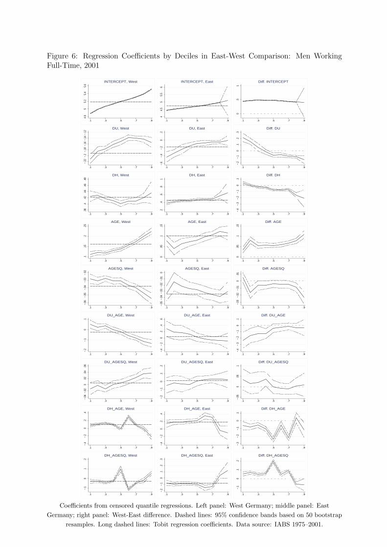
Figure 6: Regression Coefficients by Deciles in East-West Comparison: Men WorkingFull-Time, 2001
4.8
55.
25.
45.
6
.1 .3 .5 .7 .9
INTERCEPT, West
44.
55
5.5
6
.1 .3 .5 .7 .9
INTERCEPT, East
0.5
1
.1 .3 .5 .7 .9
Diff. INTERCEPT−.
22−.
2−.
18−.
16−.
14−.
12
.1 .3 .5 .7 .9
DU, West
−.6
−.4
−.2
0.2
.1 .3 .5 .7 .9
DU, East
−.2
−.1
0.1
.2.3
.1 .3 .5 .7 .9
Diff. DU
.38
.4.4
2.4
4.4
6.4
8
.1 .3 .5 .7 .9
DH, West
.2.4
.6.8
1
.1 .3 .5 .7 .9
DH, East
−.4
−.3
−.2
−.1
0.1
.1 .3 .5 .7 .9
Diff. DH
.1.1
5.2
.25
.1 .3 .5 .7 .9
AGE, West
0.0
5.1
.15
.1 .3 .5 .7 .9
AGE, East
0.0
5.1
.15
.1 .3 .5 .7 .9
Diff. AGE
−.06
−.05
−.04
−.03
−.02
.1 .3 .5 .7 .9
AGESQ, West
−.05
−.04
−.03
−.02
−.01
0
.1 .3 .5 .7 .9
AGESQ, East
−.03
−.02
−.01
0.0
1
.1 .3 .5 .7 .9
Diff. AGESQ
−.2
−.1
0.1
.1 .3 .5 .7 .9
DU_AGE, West
−.4
−.2
0.2
.4.6
.1 .3 .5 .7 .9
DU_AGE, East
−.4
−.3
−.2
−.1
0.1
.1 .3 .5 .7 .9
Diff. DU_AGE
−.04
−.02
0.0
2.0
4.0
6
.1 .3 .5 .7 .9
DU_AGESQ, West
−.2
−.1
0.1
.2
.1 .3 .5 .7 .9
DU_AGESQ, East
−.05
0.0
5.1
.1 .3 .5 .7 .9
Diff. DU_AGESQ
−.4
−.2
0.2
.4
.1 .3 .5 .7 .9
DH_AGE, West
−.4
−.2
0.2
.4
.1 .3 .5 .7 .9
DH_AGE, East
−.3
−.2
−.1
0.1
.1 .3 .5 .7 .9
Diff. DH_AGE
−.1
0.1
.2
.1 .3 .5 .7 .9
DH_AGESQ, West
−.2
−.1
0.1
.2.3
.1 .3 .5 .7 .9
DH_AGESQ, East
−.1
0.1
.2
.1 .3 .5 .7 .9
Diff. DH_AGESQ
Coefficients from censored quantile regressions. Left panel: West Germany; middle panel: EastGermany; right panel: West-East difference. Dashed lines: 95% confidence bands based on 50 bootstrap
resamples. Long dashed lines: Tobit regression coefficients. Data source: IABS 1975–2001.
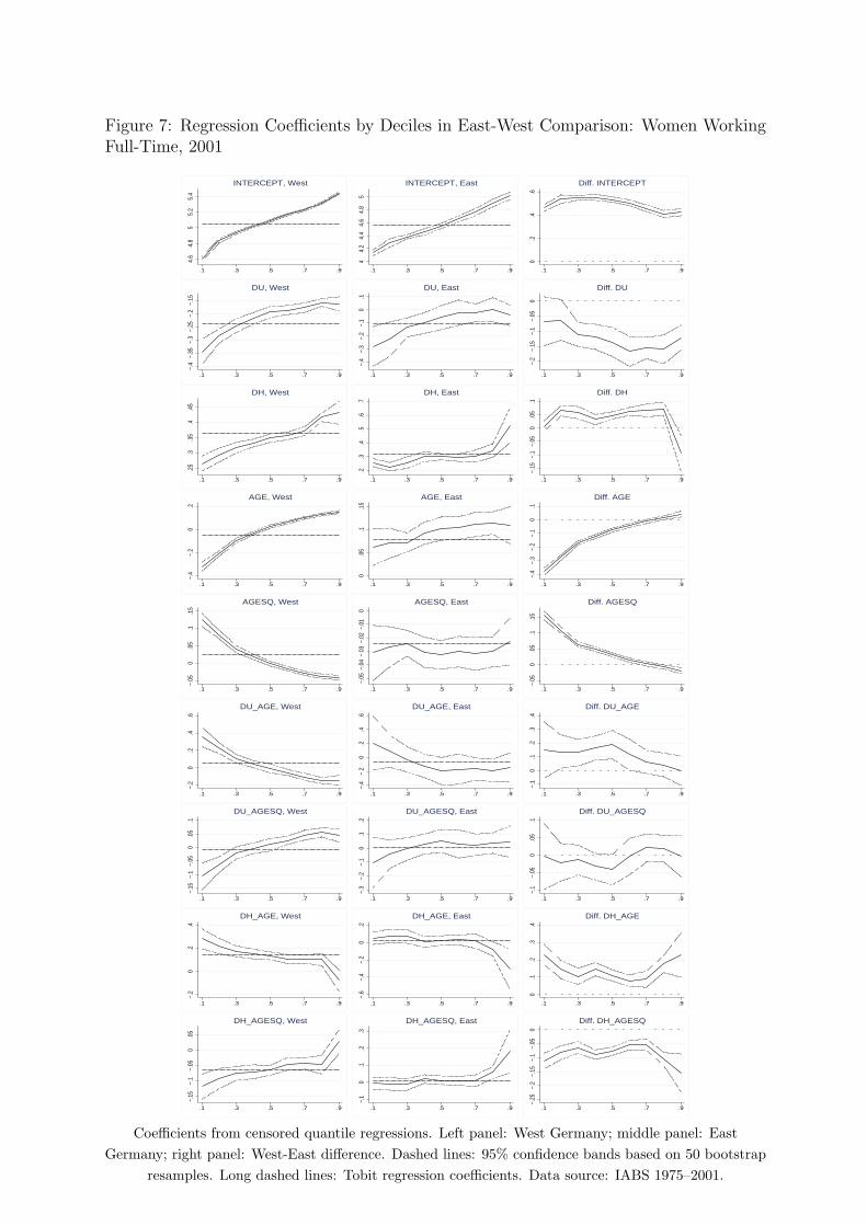
Figure 7: Regression Coefficients by Deciles in East-West Comparison: Women WorkingFull-Time, 2001
4.6
4.8
55.
25.
4
.1 .3 .5 .7 .9
INTERCEPT, West
44.
24.
44.
64.
85
.1 .3 .5 .7 .9
INTERCEPT, East
0.2
.4.6
.1 .3 .5 .7 .9
Diff. INTERCEPT−.
4−.
35−.
3−.
25−.
2−.
15
.1 .3 .5 .7 .9
DU, West
−.4
−.3
−.2
−.1
0.1
.1 .3 .5 .7 .9
DU, East
−.2
−.15
−.1
−.05
0
.1 .3 .5 .7 .9
Diff. DU
.25
.3.3
5.4
.45
.1 .3 .5 .7 .9
DH, West
.2.3
.4.5
.6.7
.1 .3 .5 .7 .9
DH, East
−.15
−.1
−.05
0.0
5.1
.1 .3 .5 .7 .9
Diff. DH
−.4
−.2
0.2
.1 .3 .5 .7 .9
AGE, West
0.0
5.1
.15
.1 .3 .5 .7 .9
AGE, East
−.4
−.3
−.2
−.1
0.1
.1 .3 .5 .7 .9
Diff. AGE
−.05
0.0
5.1
.15
.1 .3 .5 .7 .9
AGESQ, West
−.05
−.04
−.03
−.02
−.01
0
.1 .3 .5 .7 .9
AGESQ, East
−.05
0.0
5.1
.15
.1 .3 .5 .7 .9
Diff. AGESQ
−.2
0.2
.4.6
.1 .3 .5 .7 .9
DU_AGE, West
−.4
−.2
0.2
.4.6
.1 .3 .5 .7 .9
DU_AGE, East
−.1
0.1
.2.3
.4
.1 .3 .5 .7 .9
Diff. DU_AGE
−.15
−.1
−.05
0.0
5.1
.1 .3 .5 .7 .9
DU_AGESQ, West
−.3
−.2
−.1
0.1
.2
.1 .3 .5 .7 .9
DU_AGESQ, East
−.1
−.05
0.0
5.1
.1 .3 .5 .7 .9
Diff. DU_AGESQ
−.2
0.2
.4
.1 .3 .5 .7 .9
DH_AGE, West
−.6
−.4
−.2
0.2
.1 .3 .5 .7 .9
DH_AGE, East
0.1
.2.3
.4
.1 .3 .5 .7 .9
Diff. DH_AGE
−.15
−.1
−.05
0.0
5
.1 .3 .5 .7 .9
DH_AGESQ, West
−.1
0.1
.2.3
.1 .3 .5 .7 .9
DH_AGESQ, East
−.25
−.2
−.15
−.1
−.05
0
.1 .3 .5 .7 .9
Diff. DH_AGESQ
Coefficients from censored quantile regressions. Left panel: West Germany; middle panel: EastGermany; right panel: West-East difference. Dashed lines: 95% confidence bands based on 50 bootstrap
resamples. Long dashed lines: Tobit regression coefficients. Data source: IABS 1975–2001.
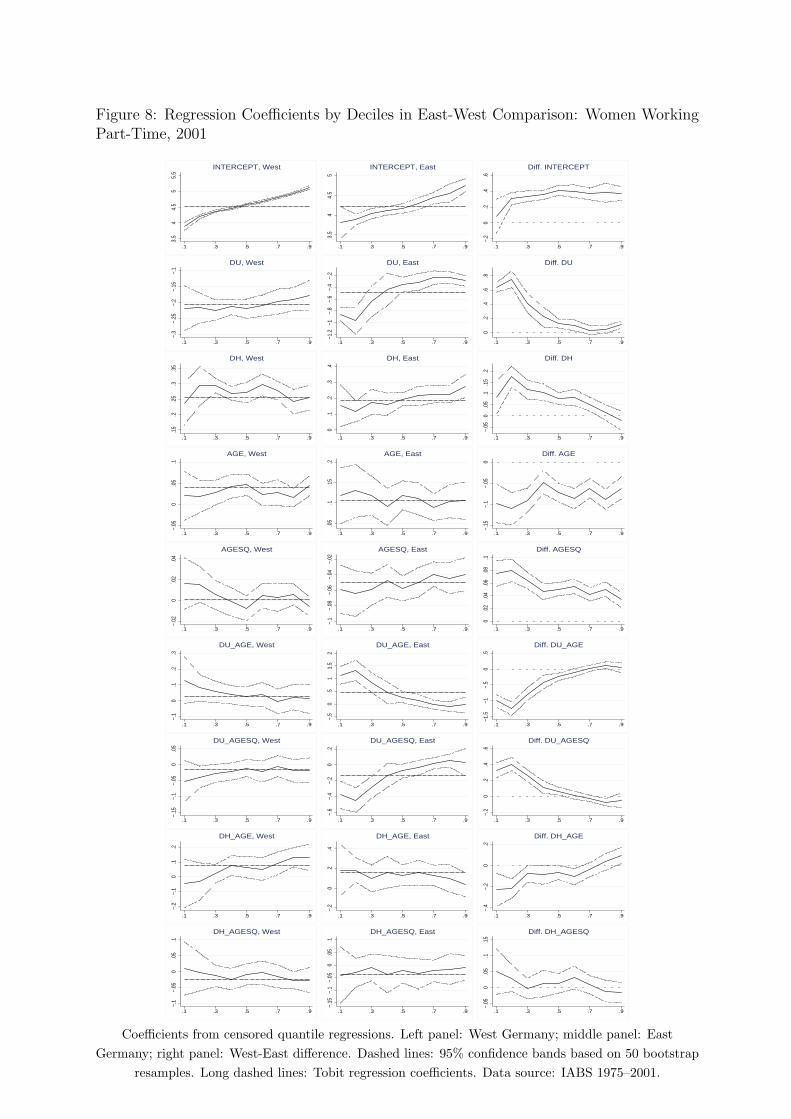
Figure 8: Regression Coefficients by Deciles in East-West Comparison: Women WorkingPart-Time, 2001
3.5
44.
55
5.5
.1 .3 .5 .7 .9
INTERCEPT, West
3.5
44.
55
.1 .3 .5 .7 .9
INTERCEPT, East
−.2
0.2
.4.6
.1 .3 .5 .7 .9
Diff. INTERCEPT−.
3−.
25−.
2−.
15−.
1
.1 .3 .5 .7 .9
DU, West
−1.2
−1−.
8−.
6−.
4−.
2
.1 .3 .5 .7 .9
DU, East
0.2
.4.6
.8
.1 .3 .5 .7 .9
Diff. DU
.15
.2.2
5.3
.35
.1 .3 .5 .7 .9
DH, West
0.1
.2.3
.4
.1 .3 .5 .7 .9
DH, East
−.05
0.0
5.1
.15
.2
.1 .3 .5 .7 .9
Diff. DH
−.05
0.0
5.1
.1 .3 .5 .7 .9
AGE, West
.05
.1.1
5.2
.1 .3 .5 .7 .9
AGE, East
−.15
−.1
−.05
0
.1 .3 .5 .7 .9
Diff. AGE
−.02
0.0
2.0
4
.1 .3 .5 .7 .9
AGESQ, West
−.1
−.08
−.06
−.04
−.02
.1 .3 .5 .7 .9
AGESQ, East
0.0
2.0
4.0
6.0
8.1
.1 .3 .5 .7 .9
Diff. AGESQ
−.1
0.1
.2.3
.1 .3 .5 .7 .9
DU_AGE, West
−.5
0.5
11.
52
.1 .3 .5 .7 .9
DU_AGE, East
−1.5
−1−.
50
.5
.1 .3 .5 .7 .9
Diff. DU_AGE
−.15
−.1
−.05
0.0
5
.1 .3 .5 .7 .9
DU_AGESQ, West
−.6
−.4
−.2
0.2
.1 .3 .5 .7 .9
DU_AGESQ, East
−.2
0.2
.4.6
.1 .3 .5 .7 .9
Diff. DU_AGESQ
−.2
−.1
0.1
.2
.1 .3 .5 .7 .9
DH_AGE, West
−.2
0.2
.4
.1 .3 .5 .7 .9
DH_AGE, East
−.4
−.2
0.2
.1 .3 .5 .7 .9
Diff. DH_AGE
−.1
−.05
0.0
5.1
.1 .3 .5 .7 .9
DH_AGESQ, West
−.15
−.1
−.05
0.0
5.1
.1 .3 .5 .7 .9
DH_AGESQ, East
−.05
0.0
5.1
.15
.1 .3 .5 .7 .9
Diff. DH_AGESQ
Coefficients from censored quantile regressions. Left panel: West Germany; middle panel: EastGermany; right panel: West-East difference. Dashed lines: 95% confidence bands based on 50 bootstrap
resamples. Long dashed lines: Tobit regression coefficients. Data source: IABS 1975–2001.

Figure 9: Regression Coefficients by Deciles in Comparison over Time: Men WorkingFull-Time, West
4.6
4.8
55.
25.
4
.1 .3 .5 .7 .9
INTERCEPT, 1992
4.8
55.
25.
45.
6
.1 .3 .5 .7 .9
INTERCEPT, 2001
0.0
5.1
.15
.2
.1 .3 .5 .7 .9
Diff. INTERCEPT−.
16−.
15−.
14−.
13−.
12−.
11
.1 .3 .5 .7 .9
DU, 1992
−.22
−.2
−.18
−.16
−.14
−.12
.1 .3 .5 .7 .9
DU, 2001
−.08
−.06
−.04
−.02
0
.1 .3 .5 .7 .9
Diff. DU
.2.2
5.3
.35
.4
.1 .3 .5 .7 .9
DH, 1992
.38
.4.4
2.4
4.4
6.4
8
.1 .3 .5 .7 .9
DH, 2001
0.0
5.1
.15
.2
.1 .3 .5 .7 .9
Diff. DH
.05
.1.1
5.2
.25
.1 .3 .5 .7 .9
AGE, 1992
.1.1
5.2
.25
.1 .3 .5 .7 .9
AGE, 2001
−.02
−.01
0.0
1.0
2
.1 .3 .5 .7 .9
Diff. AGE
−.08
−.06
−.04
−.02
0
.1 .3 .5 .7 .9
AGESQ, 1992
−.06
−.05
−.04
−.03
−.02
.1 .3 .5 .7 .9
AGESQ, 2001
−.01
0.0
1.0
2
.1 .3 .5 .7 .9
Diff. AGESQ
−.15
−.1
−.05
0.0
5
.1 .3 .5 .7 .9
DU_AGE, 1992
−.2
−.1
0.1
.1 .3 .5 .7 .9
DU_AGE, 2001
−.05
0.0
5.1
.1 .3 .5 .7 .9
Diff. DU_AGE
−.02
0.0
2.0
4
.1 .3 .5 .7 .9
DU_AGESQ, 1992
−.04
−.02
0.0
2.0
4.0
6
.1 .3 .5 .7 .9
DU_AGESQ, 2001
−.04
−.02
0.0
2.0
4
.1 .3 .5 .7 .9
Diff. DU_AGESQ
−.15
−.1
−.05
0.0
5.1
.1 .3 .5 .7 .9
DH_AGE, 1992
−.4
−.2
0.2
.4
.1 .3 .5 .7 .9
DH_AGE, 2001
−.2
−.1
0.1
.2.3
.1 .3 .5 .7 .9
Diff. DH_AGE
−.05
0.0
5.1
.15
.2
.1 .3 .5 .7 .9
DH_AGESQ, 1992
−.1
0.1
.2
.1 .3 .5 .7 .9
DH_AGESQ, 2001
−.2
−.1
0.1
.1 .3 .5 .7 .9
Diff. DH_AGESQ
Coefficients from censored quantile regressions. Left panel: 1992; middle panel: 2001; right panel:difference 2001–1992. Dashed lines: 95% confidence bands based on 50 bootstrap resamples. Long
dashed lines: Tobit regression coefficients. Data source: IABS 1975–2001.
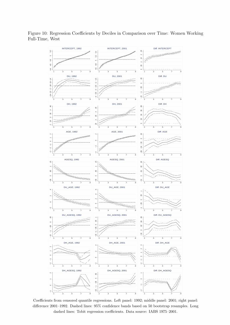
Figure 10: Regression Coefficients by Deciles in Comparison over Time: Women WorkingFull-Time, West
4.4
4.6
4.8
55.
2
.1 .3 .5 .7 .9
INTERCEPT, 1992
4.6
4.8
55.
25.
4
.1 .3 .5 .7 .9
INTERCEPT, 2001
0.0
5.1
.15
.2.2
5
.1 .3 .5 .7 .9
Diff. INTERCEPT−.
24−.
22−.
2−.
18−.
16−.
14
.1 .3 .5 .7 .9
DU, 1992
−.4
−.35
−.3
−.25
−.2
−.15
.1 .3 .5 .7 .9
DU, 2001
−.15
−.1
−.05
0.0
5
.1 .3 .5 .7 .9
Diff. DU
.2.2
5.3
.35
.4.4
5
.1 .3 .5 .7 .9
DH, 1992
.25
.3.3
5.4
.45
.1 .3 .5 .7 .9
DH, 2001
0.0
2.0
4.0
6.0
8
.1 .3 .5 .7 .9
Diff. DH
−.3
−.2
−.1
0.1
.2
.1 .3 .5 .7 .9
AGE, 1992
−.4
−.2
0.2
.1 .3 .5 .7 .9
AGE, 2001
−.06
−.04
−.02
0.0
2
.1 .3 .5 .7 .9
Diff. AGE
−.05
0.0
5.1
.15
.1 .3 .5 .7 .9
AGESQ, 1992
−.05
0.0
5.1
.15
.1 .3 .5 .7 .9
AGESQ, 2001
−.01
0.0
1.0
2.0
3
.1 .3 .5 .7 .9
Diff. AGESQ
−.2
0.2
.4
.1 .3 .5 .7 .9
DU_AGE, 1992
−.2
0.2
.4.6
.1 .3 .5 .7 .9
DU_AGE, 2001
−.1
−.05
0.0
5.1
.1 .3 .5 .7 .9
Diff. DU_AGE
−.15
−.1
−.05
0.0
5
.1 .3 .5 .7 .9
DU_AGESQ, 1992
−.15
−.1
−.05
0.0
5.1
.1 .3 .5 .7 .9
DU_AGESQ, 2001
−.02
0.0
2.0
4.0
6
.1 .3 .5 .7 .9
Diff. DU_AGESQ
−.2
−.1
0.1
.2
.1 .3 .5 .7 .9
DH_AGE, 1992
−.2
0.2
.4
.1 .3 .5 .7 .9
DH_AGE, 2001
−.2
−.1
0.1
.2.3
.1 .3 .5 .7 .9
Diff. DH_AGE
−.1
0.1
.2
.1 .3 .5 .7 .9
DH_AGESQ, 1992
−.15
−.1
−.05
0.0
5
.1 .3 .5 .7 .9
DH_AGESQ, 2001
−.2
−.1
0.1
.1 .3 .5 .7 .9
Diff. DH_AGESQ
Coefficients from censored quantile regressions. Left panel: 1992; middle panel: 2001; right panel:difference 2001–1992. Dashed lines: 95% confidence bands based on 50 bootstrap resamples. Long
dashed lines: Tobit regression coefficients. Data source: IABS 1975–2001.

Figure 11: Regression Coefficients by Deciles in Comparison over Time: Women WorkingPart-Time, West
3.5
44.
55
.1 .3 .5 .7 .9
INTERCEPT, 1992
3.5
44.
55
5.5
.1 .3 .5 .7 .9
INTERCEPT, 2001
0.1
.2.3
.4
.1 .3 .5 .7 .9
Diff. INTERCEPT−.
2−.
15−.
1−.
05
.1 .3 .5 .7 .9
DU, 1992
−.3
−.25
−.2
−.15
−.1
.1 .3 .5 .7 .9
DU, 2001
−.15
−.1
−.05
0.0
5
.1 .3 .5 .7 .9
Diff. DU
0.1
.2.3
.4
.1 .3 .5 .7 .9
DH, 1992
.15
.2.2
5.3
.35
.1 .3 .5 .7 .9
DH, 2001
−.1
−.05
0.0
5.1
.15
.1 .3 .5 .7 .9
Diff. DH
0.0
5.1
.15
.1 .3 .5 .7 .9
AGE, 1992
−.05
0.0
5.1
.1 .3 .5 .7 .9
AGE, 2001
−.15
−.1
−.05
0.0
5
.1 .3 .5 .7 .9
Diff. AGE
−.06
−.04
−.02
0.0
2
.1 .3 .5 .7 .9
AGESQ, 1992
−.02
0.0
2.0
4
.1 .3 .5 .7 .9
AGESQ, 2001
−.02
0.0
2.0
4.0
6
.1 .3 .5 .7 .9
Diff. AGESQ
−.1
0.1
.2
.1 .3 .5 .7 .9
DU_AGE, 1992
−.1
0.1
.2.3
.1 .3 .5 .7 .9
DU_AGE, 2001
−.05
0.0
5.1
.15
.2
.1 .3 .5 .7 .9
Diff. DU_AGE
−.1
−.05
0.0
5
.1 .3 .5 .7 .9
DU_AGESQ, 1992
−.15
−.1
−.05
0.0
5
.1 .3 .5 .7 .9
DU_AGESQ, 2001
−.08
−.06
−.04
−.02
0.0
2
.1 .3 .5 .7 .9
Diff. DU_AGESQ
−.2
−.1
0.1
.2.3
.1 .3 .5 .7 .9
DH_AGE, 1992
−.2
−.1
0.1
.2
.1 .3 .5 .7 .9
DH_AGE, 2001
−.3
−.2
−.1
0.1
.2
.1 .3 .5 .7 .9
Diff. DH_AGE
−.3
−.2
−.1
0.1
.1 .3 .5 .7 .9
DH_AGESQ, 1992
−.1
−.05
0.0
5.1
.1 .3 .5 .7 .9
DH_AGESQ, 2001
−.1
0.1
.2
.1 .3 .5 .7 .9
Diff. DH_AGESQ
Coefficients from censored quantile regressions. Left panel: 1992; middle panel: 2001; right panel:difference 2001–1992. Dashed lines: 95% confidence bands based on 50 bootstrap resamples. Long
dashed lines: Tobit regression coefficients. Data source: IABS 1975–2001.
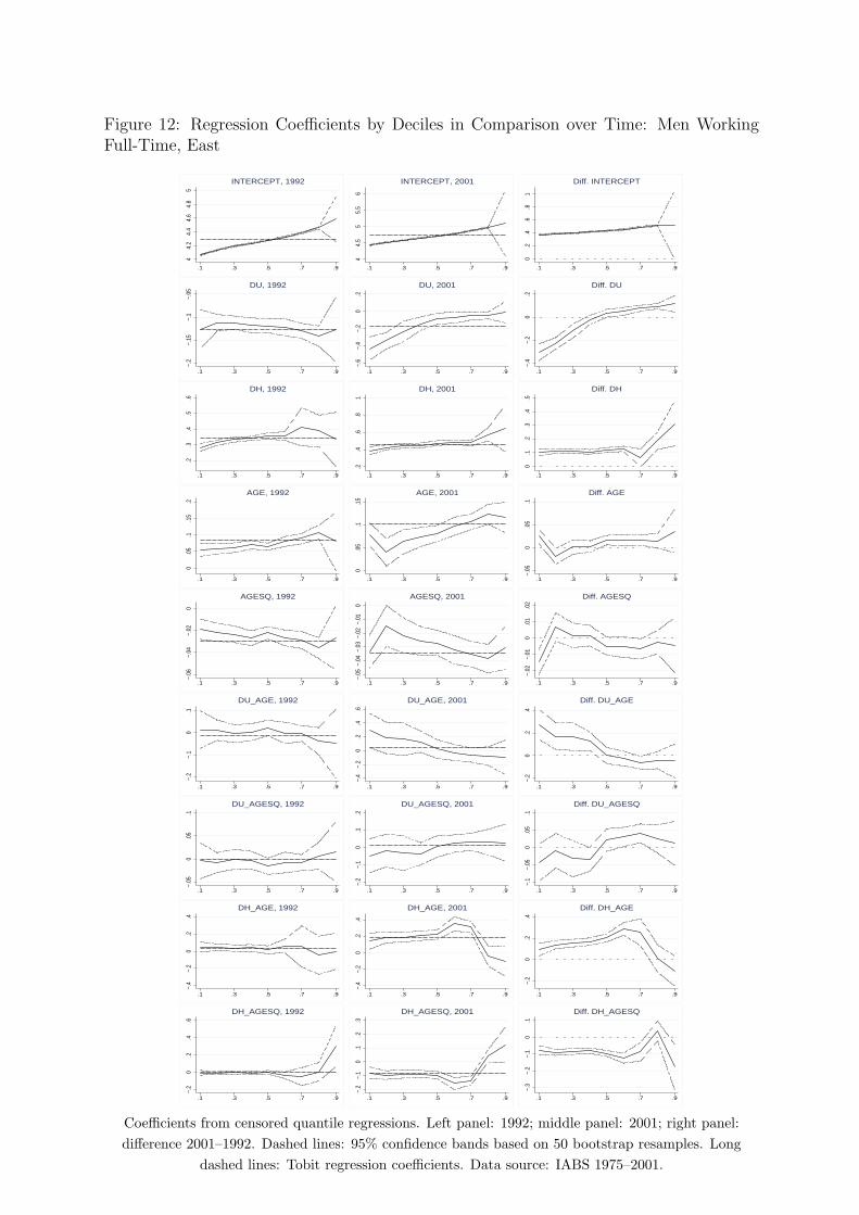
Figure 12: Regression Coefficients by Deciles in Comparison over Time: Men WorkingFull-Time, East
44.
24.
44.
64.
85
.1 .3 .5 .7 .9
INTERCEPT, 1992
44.
55
5.5
6
.1 .3 .5 .7 .9
INTERCEPT, 2001
0.2
.4.6
.81
.1 .3 .5 .7 .9
Diff. INTERCEPT−.
2−.
15−.
1−.
05
.1 .3 .5 .7 .9
DU, 1992
−.6
−.4
−.2
0.2
.1 .3 .5 .7 .9
DU, 2001
−.4
−.2
0.2
.1 .3 .5 .7 .9
Diff. DU
.2.3
.4.5
.6
.1 .3 .5 .7 .9
DH, 1992
.2.4
.6.8
1
.1 .3 .5 .7 .9
DH, 2001
0.1
.2.3
.4.5
.1 .3 .5 .7 .9
Diff. DH
0.0
5.1
.15
.2
.1 .3 .5 .7 .9
AGE, 1992
0.0
5.1
.15
.1 .3 .5 .7 .9
AGE, 2001
−.05
0.0
5.1
.1 .3 .5 .7 .9
Diff. AGE
−.06
−.04
−.02
0
.1 .3 .5 .7 .9
AGESQ, 1992
−.05
−.04
−.03
−.02
−.01
0
.1 .3 .5 .7 .9
AGESQ, 2001
−.02
−.01
0.0
1.0
2
.1 .3 .5 .7 .9
Diff. AGESQ
−.2
−.1
0.1
.1 .3 .5 .7 .9
DU_AGE, 1992
−.4
−.2
0.2
.4.6
.1 .3 .5 .7 .9
DU_AGE, 2001
−.2
0.2
.4
.1 .3 .5 .7 .9
Diff. DU_AGE
−.05
0.0
5.1
.1 .3 .5 .7 .9
DU_AGESQ, 1992
−.2
−.1
0.1
.2
.1 .3 .5 .7 .9
DU_AGESQ, 2001
−.1
−.05
0.0
5.1
.1 .3 .5 .7 .9
Diff. DU_AGESQ
−.4
−.2
0.2
.4
.1 .3 .5 .7 .9
DH_AGE, 1992
−.4
−.2
0.2
.4
.1 .3 .5 .7 .9
DH_AGE, 2001
−.2
0.2
.4
.1 .3 .5 .7 .9
Diff. DH_AGE
−.2
0.2
.4.6
.1 .3 .5 .7 .9
DH_AGESQ, 1992
−.2
−.1
0.1
.2.3
.1 .3 .5 .7 .9
DH_AGESQ, 2001
−.3
−.2
−.1
0.1
.1 .3 .5 .7 .9
Diff. DH_AGESQ
Coefficients from censored quantile regressions. Left panel: 1992; middle panel: 2001; right panel:difference 2001–1992. Dashed lines: 95% confidence bands based on 50 bootstrap resamples. Long
dashed lines: Tobit regression coefficients. Data source: IABS 1975–2001.

Figure 13: Regression Coefficients by Deciles in Comparison over Time: Women WorkingFull-Time, East
3.8
44.
24.
44.
6
.1 .3 .5 .7 .9
INTERCEPT, 1992
44.
24.
44.
64.
85
.1 .3 .5 .7 .9
INTERCEPT, 2001
0.2
.4.6
.1 .3 .5 .7 .9
Diff. INTERCEPT−.
3−.
25−.
2−.
15−.
1
.1 .3 .5 .7 .9
DU, 1992
−.4
−.3
−.2
−.1
0.1
.1 .3 .5 .7 .9
DU, 2001
−.2
−.1
0.1
.2
.1 .3 .5 .7 .9
Diff. DU
.2.2
5.3
.35
.4.4
5
.1 .3 .5 .7 .9
DH, 1992
.2.3
.4.5
.6.7
.1 .3 .5 .7 .9
DH, 2001
−.1
0.1
.2.3
.1 .3 .5 .7 .9
Diff. DH
.08
.1.1
2.1
4.1
6
.1 .3 .5 .7 .9
AGE, 1992
0.0
5.1
.15
.1 .3 .5 .7 .9
AGE, 2001
−.08
−.06
−.04
−.02
0.0
2
.1 .3 .5 .7 .9
Diff. AGE
−.07
−.06
−.05
−.04
−.03
.1 .3 .5 .7 .9
AGESQ, 1992
−.05
−.04
−.03
−.02
−.01
0
.1 .3 .5 .7 .9
AGESQ, 2001
0.0
1.0
2.0
3.0
4
.1 .3 .5 .7 .9
Diff. AGESQ
−.2
−.1
0.1
.2
.1 .3 .5 .7 .9
DU_AGE, 1992
−.4
−.2
0.2
.4.6
.1 .3 .5 .7 .9
DU_AGE, 2001
−.2
0.2
.4
.1 .3 .5 .7 .9
Diff. DU_AGE
−.1
−.05
0.0
5
.1 .3 .5 .7 .9
DU_AGESQ, 1992
−.3
−.2
−.1
0.1
.2
.1 .3 .5 .7 .9
DU_AGESQ, 2001
−.2
−.1
0.1
.1 .3 .5 .7 .9
Diff. DU_AGESQ
−.2
−.1
0.1
.2
.1 .3 .5 .7 .9
DH_AGE, 1992
−.6
−.4
−.2
0.2
.1 .3 .5 .7 .9
DH_AGE, 2001
−.6
−.4
−.2
0.2
.1 .3 .5 .7 .9
Diff. DH_AGE
−.1
−.05
0.0
5.1
.1 .3 .5 .7 .9
DH_AGESQ, 1992
−.1
0.1
.2.3
.1 .3 .5 .7 .9
DH_AGESQ, 2001
−.1
0.1
.2.3
.1 .3 .5 .7 .9
Diff. DH_AGESQ
Coefficients from censored quantile regressions. Left panel: 1992; middle panel: 2001; right panel:difference 2001–1992. Dashed lines: 95% confidence bands based on 50 bootstrap resamples. Long
dashed lines: Tobit regression coefficients. Data source: IABS 1975–2001.

Figure 14: Regression Coefficients by Deciles in Comparison over Time: Women WorkingPart-Time, East
3.2
3.4
3.6
3.8
44.
2
.1 .3 .5 .7 .9
INTERCEPT, 1992
3.5
44.
55
.1 .3 .5 .7 .9
INTERCEPT, 2001
0.2
.4.6
.8
.1 .3 .5 .7 .9
Diff. INTERCEPT−.
8−.
6−.
4−.
20
.1 .3 .5 .7 .9
DU, 1992
−1.2
−1−.
8−.
6−.
4−.
2
.1 .3 .5 .7 .9
DU, 2001
−.8
−.6
−.4
−.2
0
.1 .3 .5 .7 .9
Diff. DU
.1.2
.3.4
.5.6
.1 .3 .5 .7 .9
DH, 1992
0.1
.2.3
.4
.1 .3 .5 .7 .9
DH, 2001
−.4
−.2
0.2
.1 .3 .5 .7 .9
Diff. DH
−.05
0.0
5.1
.15
.2
.1 .3 .5 .7 .9
AGE, 1992
.05
.1.1
5.2
.1 .3 .5 .7 .9
AGE, 2001
−.05
0.0
5.1
.15
.1 .3 .5 .7 .9
Diff. AGE
−.1
−.05
0
.1 .3 .5 .7 .9
AGESQ, 1992
−.1
−.08
−.06
−.04
−.02
.1 .3 .5 .7 .9
AGESQ, 2001
−.06
−.04
−.02
0.0
2
.1 .3 .5 .7 .9
Diff. AGESQ
−.5
0.5
1
.1 .3 .5 .7 .9
DU_AGE, 1992
−.5
0.5
11.
52
.1 .3 .5 .7 .9
DU_AGE, 2001
−.5
0.5
11.
5
.1 .3 .5 .7 .9
Diff. DU_AGE
−.4
−.2
0.2
.4
.1 .3 .5 .7 .9
DU_AGESQ, 1992
−.6
−.4
−.2
0.2
.1 .3 .5 .7 .9
DU_AGESQ, 2001
−.6
−.4
−.2
0.2
.1 .3 .5 .7 .9
Diff. DU_AGESQ
−.6
−.4
−.2
0.2
.4
.1 .3 .5 .7 .9
DH_AGE, 1992
−.2
0.2
.4
.1 .3 .5 .7 .9
DH_AGE, 2001
−.2
0.2
.4.6
.1 .3 .5 .7 .9
Diff. DH_AGE
−.2
0.2
.4
.1 .3 .5 .7 .9
DH_AGESQ, 1992
−.15
−.1
−.05
0.0
5.1
.1 .3 .5 .7 .9
DH_AGESQ, 2001
−.3
−.2
−.1
0.1
.1 .3 .5 .7 .9
Diff. DH_AGESQ
Coefficients from censored quantile regressions. Left panel: 1992; middle panel: 2001; right panel:difference 2001–1992. Dashed lines: 95% confidence bands based on 50 bootstrap resamples. Long
dashed lines: Tobit regression coefficients. Data source: IABS 1975–2001.
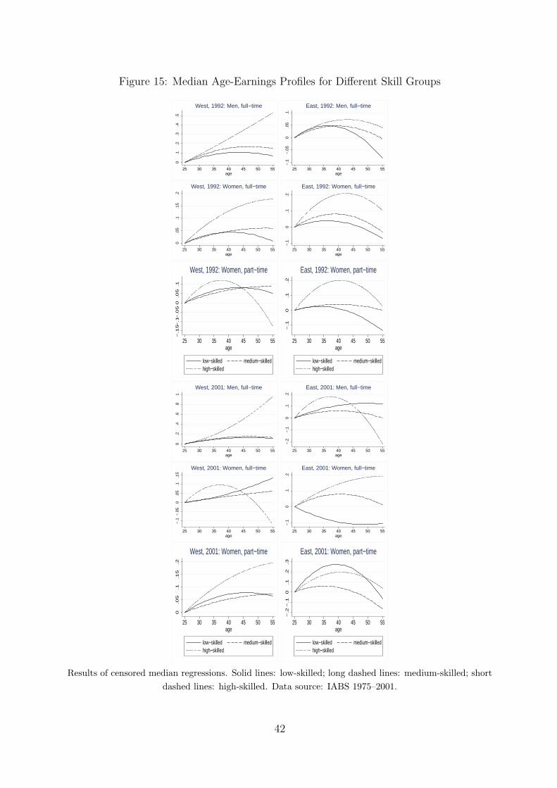
Figure 15: Median Age-Earnings Profiles for Different Skill Groups
0.1
.2.3
.4.5
25 30 35 40 45 50 55age
West, 1992: Men, full−time
−.1
−.0
50
.05
.1
25 30 35 40 45 50 55age
East, 1992: Men, full−time
0.0
5.1
.15
.2
25 30 35 40 45 50 55age
West, 1992: Women, full−time
−.1
0.1
.2
25 30 35 40 45 50 55age
East, 1992: Women, full−time
−.1
5−.1
−.0
50
.05
.1
25 30 35 40 45 50 55age
low−skilled medium−skilledhigh−skilled
West, 1992: Women, part−time
−.1
0.1
.2
25 30 35 40 45 50 55age
low−skilled medium−skilledhigh−skilled
East, 1992: Women, part−time
0.2
.4.6
.81
25 30 35 40 45 50 55age
West, 2001: Men, full−time
−.2
−.1
0.1
.2
25 30 35 40 45 50 55age
East, 2001: Men, full−time
−.1
−.0
50
.05
.1.1
5
25 30 35 40 45 50 55age
West, 2001: Women, full−time
−.1
0.1
.2
25 30 35 40 45 50 55age
East, 2001: Women, full−time
0.0
5.1
.15
.2
25 30 35 40 45 50 55age
low−skilled medium−skilledhigh−skilled
West, 2001: Women, part−time
−.2
−.1
0.1
.2.3
25 30 35 40 45 50 55age
low−skilled medium−skilledhigh−skilled
East, 2001: Women, part−time
Results of censored median regressions. Solid lines: low-skilled; long dashed lines: medium-skilled; shortdashed lines: high-skilled. Data source: IABS 1975–2001.
42
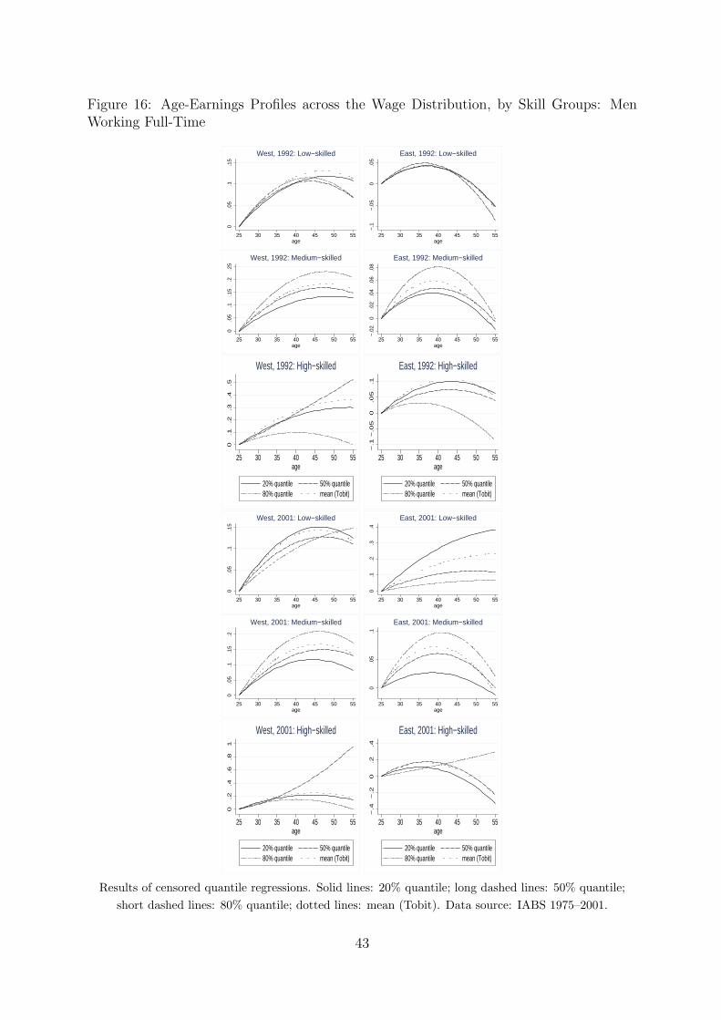
Figure 16: Age-Earnings Profiles across the Wage Distribution, by Skill Groups: MenWorking Full-Time
0.0
5.1
.15
25 30 35 40 45 50 55age
West, 1992: Low−skilled
−.1
−.0
50
.05
25 30 35 40 45 50 55age
East, 1992: Low−skilled
0.0
5.1
.15
.2.2
5
25 30 35 40 45 50 55age
West, 1992: Medium−skilled
−.0
20
.02
.04
.06
.08
25 30 35 40 45 50 55age
East, 1992: Medium−skilled
0.1
.2.3
.4.5
25 30 35 40 45 50 55age
20% quantile 50% quantile80% quantile mean (Tobit)
West, 1992: High−skilled−
.1−
.05
0.0
5.1
25 30 35 40 45 50 55age
20% quantile 50% quantile80% quantile mean (Tobit)
East, 1992: High−skilled
0.0
5.1
.15
25 30 35 40 45 50 55age
West, 2001: Low−skilled
0.1
.2.3
.4
25 30 35 40 45 50 55age
East, 2001: Low−skilled
0.0
5.1
.15
.2
25 30 35 40 45 50 55age
West, 2001: Medium−skilled
0.0
5.1
25 30 35 40 45 50 55age
East, 2001: Medium−skilled
0.2
.4.6
.81
25 30 35 40 45 50 55age
20% quantile 50% quantile80% quantile mean (Tobit)
West, 2001: High−skilled
−.4
−.2
0.2
.4
25 30 35 40 45 50 55age
20% quantile 50% quantile80% quantile mean (Tobit)
East, 2001: High−skilled
Results of censored quantile regressions. Solid lines: 20% quantile; long dashed lines: 50% quantile;short dashed lines: 80% quantile; dotted lines: mean (Tobit). Data source: IABS 1975–2001.
43
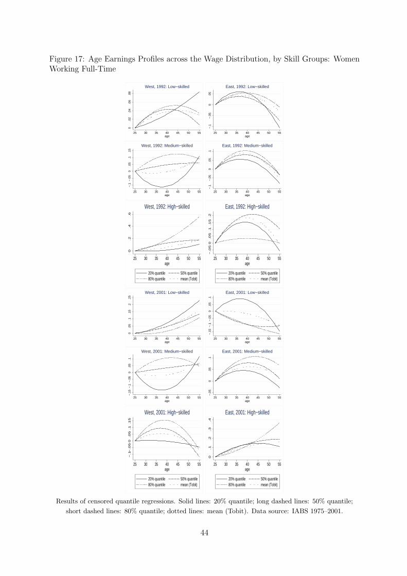
Figure 17: Age Earnings Profiles across the Wage Distribution, by Skill Groups: WomenWorking Full-Time
0.0
2.0
4.0
6.0
825 30 35 40 45 50 55
age
West, 1992: Low−skilled
−.1
−.0
50
.05
25 30 35 40 45 50 55age
East, 1992: Low−skilled
−.1
−.0
50
.05
.1.1
5
25 30 35 40 45 50 55age
West, 1992: Medium−skilled
−.1
−.0
50
.05
.1
25 30 35 40 45 50 55age
East, 1992: Medium−skilled
0.2
.4.6
25 30 35 40 45 50 55age
20% quantile 50% quantile80% quantile mean (Tobit)
West, 1992: High−skilled−
.05
0.0
5.1
.15
.2
25 30 35 40 45 50 55age
20% quantile 50% quantile80% quantile mean (Tobit)
East, 1992: High−skilled
0.0
5.1
.15
.2.2
5
25 30 35 40 45 50 55age
West, 2001: Low−skilled
−.1
5−
.1−
.05
0.0
5.1
25 30 35 40 45 50 55age
East, 2001: Low−skilled
−.1
5−
.1−
.05
0.0
5.1
25 30 35 40 45 50 55age
West, 2001: Medium−skilled
−.0
50
.05
.1
25 30 35 40 45 50 55age
East, 2001: Medium−skilled
−.1
−.0
50
.05
.1.1
5
25 30 35 40 45 50 55age
20% quantile 50% quantile80% quantile mean (Tobit)
West, 2001: High−skilled
0.1
.2.3
.4
25 30 35 40 45 50 55age
20% quantile 50% quantile80% quantile mean (Tobit)
East, 2001: High−skilled
Results of censored quantile regressions. Solid lines: 20% quantile; long dashed lines: 50% quantile;short dashed lines: 80% quantile; dotted lines: mean (Tobit). Data source: IABS 1975–2001.
44
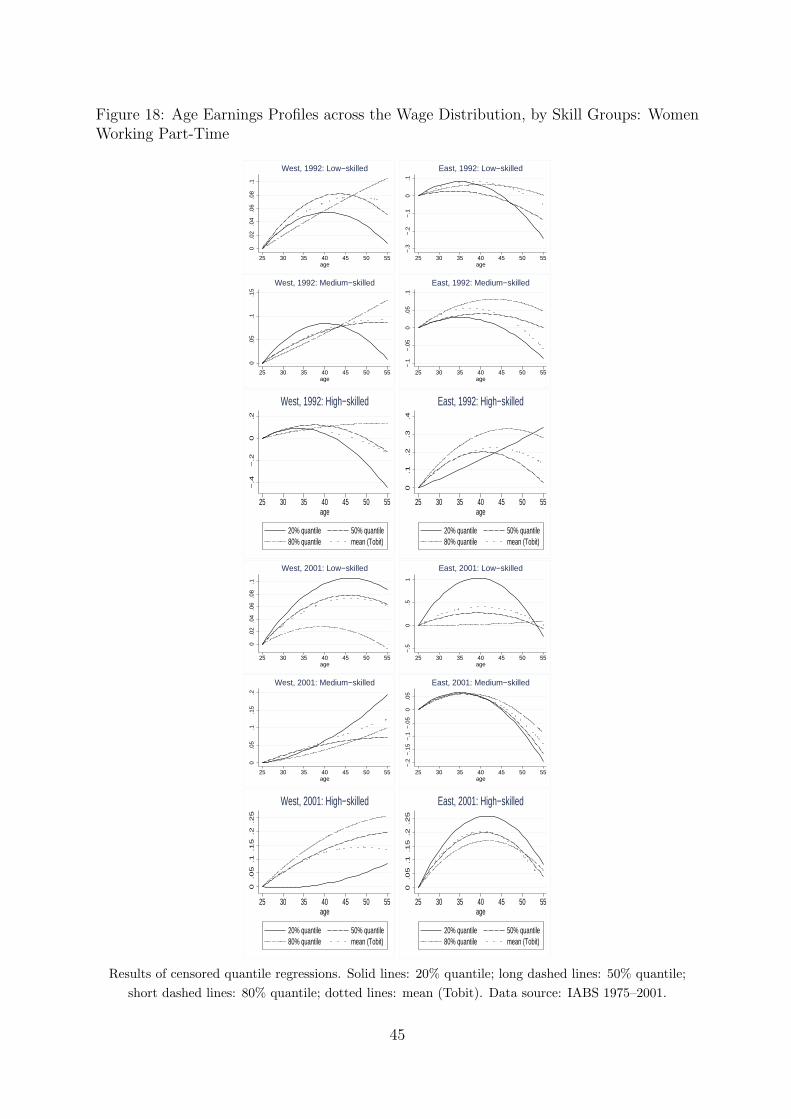
Figure 18: Age Earnings Profiles across the Wage Distribution, by Skill Groups: WomenWorking Part-Time
0.0
2.0
4.0
6.0
8.1
25 30 35 40 45 50 55age
West, 1992: Low−skilled
−.3
−.2
−.1
0.1
25 30 35 40 45 50 55age
East, 1992: Low−skilled
0.0
5.1
.15
25 30 35 40 45 50 55age
West, 1992: Medium−skilled
−.1
−.0
50
.05
.1
25 30 35 40 45 50 55age
East, 1992: Medium−skilled
−.4
−.2
0.2
25 30 35 40 45 50 55age
20% quantile 50% quantile80% quantile mean (Tobit)
West, 1992: High−skilled0
.1.2
.3.4
25 30 35 40 45 50 55age
20% quantile 50% quantile80% quantile mean (Tobit)
East, 1992: High−skilled
0.0
2.0
4.0
6.0
8.1
25 30 35 40 45 50 55age
West, 2001: Low−skilled
−.5
0.5
1
25 30 35 40 45 50 55age
East, 2001: Low−skilled
0.0
5.1
.15
.2
25 30 35 40 45 50 55age
West, 2001: Medium−skilled
−.2
−.1
5−
.1−
.05
0.0
5
25 30 35 40 45 50 55age
East, 2001: Medium−skilled
0.0
5.1
.15
.2.2
5
25 30 35 40 45 50 55age
20% quantile 50% quantile80% quantile mean (Tobit)
West, 2001: High−skilled
0.0
5.1
.15
.2.2
5
25 30 35 40 45 50 55age
20% quantile 50% quantile80% quantile mean (Tobit)
East, 2001: High−skilled
Results of censored quantile regressions. Solid lines: 20% quantile; long dashed lines: 50% quantile;short dashed lines: 80% quantile; dotted lines: mean (Tobit). Data source: IABS 1975–2001.
45
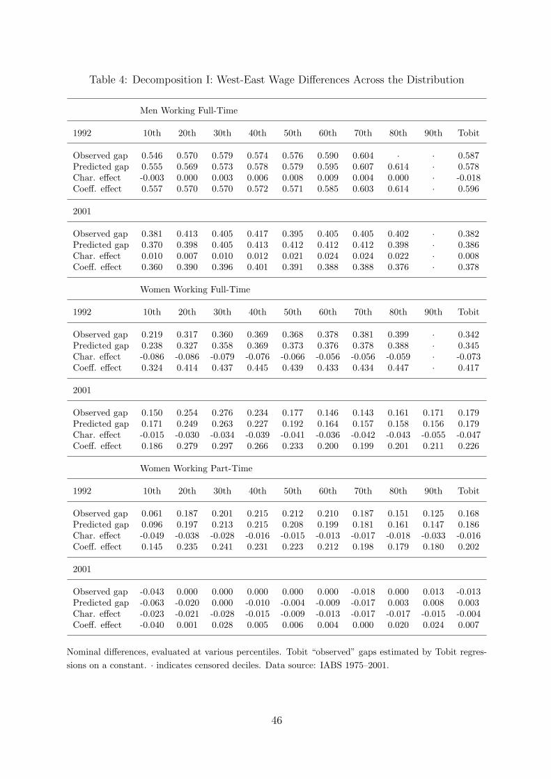
Table 4: Decomposition I: West-East Wage Differences Across the Distribution
Men Working Full-Time
1992 10th 20th 30th 40th 50th 60th 70th 80th 90th Tobit
Observed gap 0.546 0.570 0.579 0.574 0.576 0.590 0.604 · · 0.587Predicted gap 0.555 0.569 0.573 0.578 0.579 0.595 0.607 0.614 · 0.578Char. effect -0.003 0.000 0.003 0.006 0.008 0.009 0.004 0.000 · -0.018Coeff. effect 0.557 0.570 0.570 0.572 0.571 0.585 0.603 0.614 · 0.596
2001
Observed gap 0.381 0.413 0.405 0.417 0.395 0.405 0.405 0.402 · 0.382Predicted gap 0.370 0.398 0.405 0.413 0.412 0.412 0.412 0.398 · 0.386Char. effect 0.010 0.007 0.010 0.012 0.021 0.024 0.024 0.022 · 0.008Coeff. effect 0.360 0.390 0.396 0.401 0.391 0.388 0.388 0.376 · 0.378
Women Working Full-Time
1992 10th 20th 30th 40th 50th 60th 70th 80th 90th Tobit
Observed gap 0.219 0.317 0.360 0.369 0.368 0.378 0.381 0.399 · 0.342Predicted gap 0.238 0.327 0.358 0.369 0.373 0.376 0.378 0.388 · 0.345Char. effect -0.086 -0.086 -0.079 -0.076 -0.066 -0.056 -0.056 -0.059 · -0.073Coeff. effect 0.324 0.414 0.437 0.445 0.439 0.433 0.434 0.447 · 0.417
2001
Observed gap 0.150 0.254 0.276 0.234 0.177 0.146 0.143 0.161 0.171 0.179Predicted gap 0.171 0.249 0.263 0.227 0.192 0.164 0.157 0.158 0.156 0.179Char. effect -0.015 -0.030 -0.034 -0.039 -0.041 -0.036 -0.042 -0.043 -0.055 -0.047Coeff. effect 0.186 0.279 0.297 0.266 0.233 0.200 0.199 0.201 0.211 0.226
Women Working Part-Time
1992 10th 20th 30th 40th 50th 60th 70th 80th 90th Tobit
Observed gap 0.061 0.187 0.201 0.215 0.212 0.210 0.187 0.151 0.125 0.168Predicted gap 0.096 0.197 0.213 0.215 0.208 0.199 0.181 0.161 0.147 0.186Char. effect -0.049 -0.038 -0.028 -0.016 -0.015 -0.013 -0.017 -0.018 -0.033 -0.016Coeff. effect 0.145 0.235 0.241 0.231 0.223 0.212 0.198 0.179 0.180 0.202
2001
Observed gap -0.043 0.000 0.000 0.000 0.000 0.000 -0.018 0.000 0.013 -0.013Predicted gap -0.063 -0.020 0.000 -0.010 -0.004 -0.009 -0.017 0.003 0.008 0.003Char. effect -0.023 -0.021 -0.028 -0.015 -0.009 -0.013 -0.017 -0.017 -0.015 -0.004Coeff. effect -0.040 0.001 0.028 0.005 0.006 0.004 0.000 0.020 0.024 0.007
Nominal differences, evaluated at various percentiles. Tobit “observed” gaps estimated by Tobit regres-sions on a constant. · indicates censored deciles. Data source: IABS 1975–2001.
46
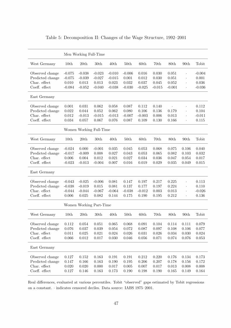
Table 5: Decomposition II: Changes of the Wage Structure, 1992–2001
Men Working Full-Time
West Germany 10th 20th 30th 40th 50th 60th 70th 80th 90th Tobit
Observed change -0.075 -0.038 -0.023 -0.010 -0.006 0.016 0.030 0.051 · -0.004Predicted change -0.075 -0.039 -0.027 -0.015 0.001 0.012 0.030 0.051 · 0.001Char. effect 0.010 0.013 0.013 0.023 0.032 0.037 0.045 0.052 · 0.036Coeff. effect -0.084 -0.052 -0.040 -0.038 -0.030 -0.025 -0.015 -0.001 · -0.036
East Germany
Observed change 0.001 0.031 0.062 0.058 0.087 0.112 0.140 · · 0.112Predicted change 0.022 0.044 0.052 0.062 0.080 0.106 0.136 0.179 · 0.104Char. effect 0.012 -0.013 -0.015 -0.013 -0.007 -0.003 0.006 0.013 · -0.011Coeff. effect 0.034 0.057 0.067 0.076 0.087 0.109 0.130 0.166 · 0.115
Women Working Full-Time
West Germany 10th 20th 30th 40th 50th 60th 70th 80th 90th Tobit
Observed change -0.024 0.000 -0.001 0.035 0.045 0.053 0.068 0.075 0.106 0.040Predicted change -0.017 -0.009 0.008 0.027 0.043 0.053 0.065 0.082 0.103 0.032Char. effect 0.006 0.004 0.012 0.021 0.027 0.034 0.036 0.047 0.054 0.017Coeff. effect -0.023 -0.013 -0.004 0.007 0.016 0.019 0.029 0.035 0.049 0.015
East Germany
Observed change -0.043 -0.025 -0.006 0.081 0.147 0.197 0.217 0.225 · 0.113Predicted change -0.038 -0.019 0.015 0.081 0.137 0.177 0.197 0.224 · 0.110Char. effect -0.044 -0.044 -0.067 -0.064 -0.038 -0.012 0.003 0.013 · -0.026Coeff. effect 0.006 0.025 0.082 0.144 0.175 0.190 0.195 0.212 · 0.136
Women Working Part-Time
West Germany 10th 20th 30th 40th 50th 60th 70th 80th 90th Tobit
Observed change 0.112 0.054 0.051 0.065 0.068 0.091 0.104 0.114 0.111 0.079Predicted change 0.076 0.037 0.039 0.054 0.072 0.087 0.097 0.108 0.106 0.077Char. effect 0.011 0.025 0.021 0.024 0.026 0.031 0.026 0.034 0.030 0.024Coeff. effect 0.066 0.012 0.017 0.030 0.046 0.056 0.071 0.074 0.076 0.053
East Germany
Observed change 0.127 0.152 0.163 0.191 0.191 0.212 0.220 0.176 0.134 0.173Predicted change 0.147 0.166 0.163 0.190 0.195 0.206 0.207 0.178 0.156 0.172Char. effect 0.020 0.020 0.000 0.017 0.005 0.007 0.017 0.013 0.008 0.008Coeff. effect 0.127 0.146 0.163 0.173 0.190 0.198 0.190 0.165 0.149 0.164
Real differences, evaluated at various percentiles. Tobit “observed” gaps estimated by Tobit regressionson a constant. · indicates censored deciles. Data source: IABS 1975–2001.
47
Related Documents