Rigid-body pose and twist estimation using an accelerometer array

Archive of Applied Mechanics 74 (2004) 223-236 �9 Springer-Veflag 2004 DOI lo.loo7/soo419-oo4-o345-6

Rigid-body pose and twist estimation using an accelerometer array

K. Parsa, J. Angeles, A. K. Misra

Summary A novel technique for the determination of the pose and the twist of rigid bodies using point-acceleration data is proposed. These data are collected from an accelerometer array, which is a kinematically redundant set of triaxial accelerometers. Because orientational error in the installation of the accelerometers can be fatal to the accuracy of the results, a calibration procedure based on the consistency of the point accelerations is outlined. The formulation developed is then utilized in the simulation analysis of two sample motions. The relations required to estimate the pose and the twist are derived in a body-fixed frame. The body angular acceleration and angular velocity, in this order, are determined directly from the acceleration data; the body attitude is then computed through integration.

Keywords Accelerometer, gyroscope-free inertial navigation, pose and twist

1 Introduction The real-time estimation of the pose and the twist of rigid bodies has been the focus of research for several decades. (By pose we mean the position and the orientation of the rigid body, and by twist the velocity and the angular velocity of the rigid body is meant). The principal reason for this interest was perhaps, its application in the guidance and navigation of aircraft, spacecraft, and satellites. However, new applications are being found in the realm of robotics and auto- mation; all mobile robots are equipped with systems that can help determine their pose and twist, for example.

In inertial navigation systems, accelerometers have long been used beside other types of sensors, such as rate-gyros, inclinometers, or combinations thereof, for dead reckoning. In such a system, the rate-gyro is used to measure the absolute angular velocity, upon the numerical integration of which the body attitude is obtained. Then, by reading the acceler- ometer signals, the navigation system can determine an inertial-frame representation of the absolute acceleration of the body, [9]. Next, this acceleration is integrated to infer the full twist and pose of the body. Such an approach has been used in a number of works, e.g., in [5, 10, 18, 21], to name a few.

The determination of the angular-velocity vector of a rigid-body from the velocity data of three noncollinear points of the body was studied in [1]. Then, in a related work, [2], the same

Received 4 March 2004; accepted for publication 14 June 2004

K. Parsa (~J) Currently Visiting Fellow, Space Technologies Canadian Space Agency 6767 route de I'Aeroport Saint-Hubert, Qc ]3Y 8Y9 Canada e-mail: [email protected]

J. Angeles, A. K. Misra Department of Mechanical Engineering and Centre for Intelligent Machines, McGill University, 817 Sherbrooke St. W., Montreal, QC, Canada H3A 2K6 e-mail: [email protected], [email protected]

This research work was supported by the Natural Sciences and Engineering Research Council of Canada, under Research Grants OGP0004532 and OGP0000967.

223

224

author discussed the determination of the angular-acceleration using the velocity and accel- eration information of three noncoUinear points of the body; the results were then extended to the redundant-measurement case, for which the underlying compatibility relations were ob- tained. Apparently, having the angular acceleration of the body, one can compute the body angular velocity through integration, which would cause cumulative angular-velocity error.

Since measurements are unavoidably contaminated by noise, a pose- and twist-estimation algorithm was developed, [3], that filtered the noise content of the pose- and twist-measure- ment signals through a least-square approach. Later, the results of [2] were generalized, [19], to cases whereby statistical weighting is desired. Even though the estimation of pose, twist, and angular acceleration of a rigid-body was the subject of these four works, it was assumed that the data were available in a fixed reference frame.

Other researchers, [11, 13], have solved the problem of angular-acceleration determination under the assumption that only one acceleration component of different points of the body are known. It has been reported in [13] that, to be able to determine both translational and angular accelerations of a rigid-body, only six single-axis accelerometers are needed; furthermore, the solution becomes easier by adding three extra accelerometers to the array of accelerometers. However, in both these cases, the angular velocity of the body has to be computed through integration. A similar idea has been used in a number of gyroscope-free inertial navigation system designs aided by the Global Positioning System, [6, 12, 20].

The problem of pose and twist estimation using a kinematically redundant--i.e., more than three--array of triaxial accelerometers, which is called an accelerometer array, was discussed in [15]. Considering the possibility of accelerometers having installation error in their orientation, the authors showed that orientation errors as small as 0.1 ~ can cause even the angular-velocity estimate, obtained by integrating the angular acceleration, to rapidly diverge from its actual value, thereby completely undermining the accuracy of the results.

To overcome the problem of orientational installation error, one can put the array at given attitudes, and then measure the gravitational acceleration. The results are then used to identify the accelerometer axes, [6]. One such algorithm using redundant measurements was discussed in [16]. This type of calibration, however, is imperfect as its accuracy is dependent upon the accuracy of the attitudes at which the measurements are made.

In this paper, a calibration scheme which is based on the consistency of point-acceleration data is proposed. It will be shown here that the scheme is capable of identifying accelerometer- attitude errors with high accuracy. Moreover, we propose a novel formulation for pose and twist estimation, through which the angular velocity and angular acceleration are determined directly from the accelerometer data in closed form.

The paper is organized as follows: The underlying kinematic relations through which the pose and the twist can be estimated from the accelerometer-array signals are the subject of Sec. 2. The attitude-calibration scheme, which is based on the compatibility of the rigid-body point-acceleration measurements, is explained in Sec. 3. Some simulation results are reported in Sec. 4. The issue of the real-time applicability of our methods is addressed in Sec. 5, the paper concluding in Sec. 6.

Throughout this paper, all vectors and cross-product matrices are expressed in their local frames, unless otherwise specified by use of a left-superscript. For exam~..le, while Pi represents the position vector of the origin of the body-frame o~/i expressed in J i , ~ Pi is the same position vector expressed in the inertial frame ~. Furthermore, overdots represent element-wise dif- ferentiation of a vector array with respect to time.

2 Accelerometer-array kinematics Assume that a triaxial accelerometer is attached at each of the pickup points Pi(i = 1 ,2 , . . . , m), with position vectors Pi of the rigid body shown in Fig. 1; point C, having position vector

1 m

c = - - } , p i ,

is the centroid of {Pi}~. Obviously, due to installation errors, not only are the accelerometer axes skewed with

respect to their nominal installation orientations but also the accelerometers are located at points different from the nominal ones specified by the relative position vectors ri. The effect of the latter is minimized by choosing Ilri[[ considerably larger than the upper bound of the

Am

/ / Fig. 1. A rigid body and its related frames

225

existing position errors, and by choosing Pi to be the vertices of a Platonic solid, [3]. Here, we further assume that the three accelerometer axes are mutually orthogonal.

Assuming that an estimate t)i of the actual rotation matrix Q~,~,, from the ith accelerometer frame to the body frame is known, one can relate the two through a third rotation matrix t)i representing the calibration error as

Q~.#, -- QiOi, i = 1 , 2 , . . . , m . (1)

The calibration error can be calculated as, [4],

(~i = ee~iEi ~ 1 + s i n ~iEi + (1 - - COS ~ i ) E ~ , (2)

where ~b i and Ei are the angular error and the cross-product matrix of the unit vector ei lying along the orientational-error axis, respectively, 1 being the 3 x 3 identity matrix. Notice that the cross-product matrix V of a vector v, not dependent upon x, is the skew-symmetric matrix given by

v - CPM(v)~ O ( ~ x ) , Vx c ~3 ~ Vx - v • x . (3)

Unfortunately, however, both tki and Ei are unknown constants. Because of the preliminary calibration of the array, all ~b i can be assumed small, and hence,

the right-hand side of Eq. (2) can be approximated linearly as

Oi ~ 1 + flPiEi, i ---- 1, 2 , . . . , m . (4)

2.1 Angular acceleration From rigid-body kinematics, the absolute acceleration ai of Pi and that of the centroid, denoted by ac, are related by

a i : a c + 0 ~ • r i + ~ o • (a~ x ri) , (5)

in which to and ~t are the body angular velocity and angular acceleration, respectively. Neglecting the accelerometer bias, this acceleration in terms of the accelerometer signals '~r is given by

a i : Q:~,~, ( '~iai + ' ~ i g ) , (6)

with g representing the gravitational acceleration. The element-wise time derivative of the angular velocity of a body in its local frame, however, is exactly equal to its absolute angular acceleration expressed in the same frame, [15], i.e.,

& = ~ . (7)

Therefore, using the cross-product matrices ~ and ~ of to and &, respectively, one can rewrite Eq. (5) in a more suitable form

ai--ac----- ( ~ + ~ 2 ) r i �9 (8)

Moreover, using Eqs. (1 & 6), and recalling the definition of C, one can calculate the left- hand side of Eq. (8) as

2 2 6 1 m

ai - ac = (~iOi(~r + ~/'g) - m ~ (~jQj('~/Jaj + ~/Jg) j l "~

.= OiOiJ ia i _ _1 ~ QjQf~r m j=l

= a~ + n a , (9)

r and n a, after utilizing Eq. (4), are defined as in which a i

1 m ^

a r zx ~ .~r __ ~ i = "(i ai m Qj'~CJaj (lO)

^ a A c ~ i Q i E i J , a i _ __1 qbjQjEj,~lja j .

n i = m j = l (11)

Note that, even though the gravitational acceleration g must be added to each of the acceler- ometer measurements in order to obtain the acceleration of the corresponding pickup point, this effect vanishes in ai - ac, no matter how accurate, or inaccurate for that matter, the calibration is. Of course, the less accurate the calibration, the larger the norm [[na[[, which, in turn, affects the accuracy of the final results.

Furthermore, let us define the 3 • m matrices R, Ar, and Na as

R~[ r l r2 . . . rm] , (12)

Ar~[a~ a ~ . . . a r ] , (13)

Na~[n~ n ~ . . . n a ] . (14)

Then, by equating the right-hand sides of Eqs. (8 & 9), assembling all the equations in matrix form, and noticing the definitions given by Eqs. (10-14), one can write

WR = Ar + Na , (15)

in which, by definition, the angular-acceleration tensor W is given by

(16)

Hence, the least-square solution of Eq. (15) is

W = (Ar + Na)R t, Rt~RT(RRT) -1 , (17)

in which the Moore-penrose generalized inverse R~ of matrix R need be calculated only once. Since ~ and f~2 are skew-symmetric and symmetric, respectively, one can readily calculate

the angular acceleration of the body by taking the axial vector of the estimate ~" of W, namely,

= vect(W) ,

where the axial vector of a real, 3 • 3 matrix V = [vii] is defined as

I IT v = v e c t ( V ) : ~ v32 - v23 vl3 - v31 v21 - v12

Matrix W used in Eq. (18) is computed using Eq. (17) while neglecting N a, i.e.,

---- ArRT(RRT) -1

(18)

(19)

(20) 2 2 7

2.2 Angular velocity The calculation of the angular velocity from ~2, however, is not as straightforward as that of the angular acceleration when there is a substantial calibration error. The reason is that, in such a case, there are six inconsistent second-order equations in three unknowns. Therefore, solving them, i.e., calculating the best estimate for the angular-velocity vector, requires an optimum estimation scheme, which can be computationally expensive; moreover, the result will not necessarily be consistent with the angular acceleration calculated from Eq, (18). Our simula- tions demonstrate that, in the presence of calibration errors, the numerical integration of the angular acceleration alone will provide results suitable enough for the highly accurate cali- bration method proposed here.

After the installation errors are identified and accounted for, however, the angular velocity can be determined quite accurately from f~2 either by using a numerical procedure such as Newton-Raphson's (NR), as suggested in [16], or in closed form, as explained below.

Because f~2 can be written as, [14],

-[Io llZl § T , (21)

the system of nonlinear equations to be solved for oJ is given by

-II,o1121 + = Ws , (22)

where Ws is the symmetric part of the angular-acceleration tensor, i.e.,

^ , x l ^ Ws = ~ (W + "v~ rr) . (23)

Upon taking the trace of both sides of Eq. (22), one obtains

1 tr(' s) . (24) II~ = 2

As a result, Eq. (22) can be rewritten as

1 ^ oJoff = T~r s - ~ t r(Ws)l , (25)

from which, by taking the square root of the diagonal elements of the foregoing 3 • 3 matrix equation, the components of oJ are obtained up to a sign uncertainty; the correct sign can be determined by looking at the sign of the components of the approximate value of oJ at the (i + 1)-st sampling time obtained using Simpson's rule, namely,

r = (/~i -~- h ( s 4 - ~i) , (26)

with h representing the sampling period.

228

Obviously, the norm of the angular velocity cannot be negative. However, when the angular velocity is at the verge of vanishing, the trace in Eq. (24) can become positive due to round-off or measurement errors. In such cases, one has to assume the trace to be zero. The same has to be done when any of the diagonal elements of the right-hand side of Eq. (25) becomes negative. In other words, the method explained here loses accuracy when the angular-velocity compo- nents go through a sign change or when they become zero and remain so.

As seen from Eq. (18), using the procedure outlined here, one can calculate the angular acceleration of the body without a priori knowledge of the body angular velocity; neither does the procedure require integration of the angular acceleration. These features bring about a major accuracy improvement when compared with the procedure proposed in [15].

2.3 Translational velocity and position Using elementary kinematics, it can be shown that the element-wise time-rate of the centroid velocity Vc is given by

Vc = ac -g2Vc , (27)

and

~: = vc - ~c. (28)

Integrating the two above relations, given the initial conditions, one can obtain Vc and c. Of course, in the absence of direct measurements of the velocity and position, these vectors should be seen as unobservable; as such, the estimation errors are expected to grow without bounds, [17].

2.4 The rigid-body attitude The attitude of a rigid body can be expressed using many different three- or four-parameter representations, [4, 8, 22], among which Euler parameters have proven to be the best regarding the ease of algebraic manipulation, algebraic robustness, and ease of integration into the dynamics models of rigid bodies.

The Euler parameters constitute a set of unit quaternions and can be expressed as a unit four-dimensional array t/, given by

[ ] [ T __(~ COS q = u Tuo & e Ts in2 (29)

where u and u0 are the vector and the scalar parts of the Euler-parameter array, respectively. The foregoing equation defines the two parts in terms of the rotation angle (p and rotation-axis unit vector e. This representation means that the rigid body has arrived at its new attitude, from a reference orientation, via a rotation through an angle q~ about an axis parallel to the unit vector e. This rotation can also be represented by the rotation matrix Q given by, [4],

Q = 1 + 2 u o U + 2 U 2 , (30)

where U-~ CPM(u). The time-rate of change of the Euler parameters in the body-frame is related to the angular

velocity of the body, expressed in the same frame by, [14],

/ / = K(m)F/ , (31a)

l[. o] K-- K ( r - ~ r (31b)

One may be tempted to find the solution of this differential equation in closed-form as

However, this solution can be correct only if the two matrices exp (ft Kdt) and K commute under multiplication, which is not always the case.

Therefore, Eq. (3 la) is integrated numerically to compute the orientation of the body. Due to truncation and round-off errors, however, the result of the integration at each time-step most likely will not be consistent, i.e, the norm of q most likely will fail to be unity. To overcome this problem, one can find a least-square-error approximation by normalizing the quaternion thus obtained, i.e., by replacing q by q/Jlqll at each time step. The reason is that the normal projection of any given point in the four-dimensional euclidean space onto the unit hyper- sphere yields the closest point on the hypersphere to the given point.

It has been proven in [7] that, if the non-normalized quaternion is used to calculate a corresponding non-orthogonal rotation matrix from Eq. (30), then the orthogonalization of this matrix through the polar-decomposition theorem yields an orthogonal matrix which is exactly the same as the rotation matrix corresponding to the normalized quaternion.

Hence, the system of differential equations to be integrated to estimate the pose and twist of the rigid body is composed of Eqs. (27, 28, 31a). The important feature of these equations is that, since they are all written in the body-frame, no knowledge of the body attitude is required for the calculation of the twist. Consequently, the error incurred at the pose-estimation level does not propagate back to the twist-estimation level, although it causes inaccuracies in the reference-frame representation of the twist.

3 ginematic attitude calibration As will be seen in Sec. 4, due to gravitational calibration errors, the integration results are not stable even in the presence of small angular errors; in fact, the estimation errors for any of the pose and twist components, as well as the rate at which these errors grow, increase with the calibration errors. Therefore, to remedy the situation and to obtain a better estimate of the actual value of the states, a second calibration scheme, not requiring an accurate knowledge of the accelerometer-array pose, is needed to estimate the calibration-error rotation matrices (~i. One such scheme is proposed in this section.

Firstly, vectors ei are defined as

e i ~ i e i , i = 1 , 2 , . . . , m . (32)

229

Using these definitions, n~, given by Eq. (11), can be rewritten as

a :_ QiEi .4 ia i_ 1 ~ OjEj.~C)aj ni m j = l (33)

where Ei&CPM(ei). Then, from Eq. (15), an estimate lq, of matrix Na of Eq. (14) is evaluated from

l~ a = W R -- A r (34)

in which W is given by Eq. (20). Calculating Na, one can obtain an approximate value for n a by just picking up the ith column

of Na. On the other hand, from Eq. (33), it can be seen that

1 m ^ m 1 - - m QjAjej " QiAiei + = n i , m ._

J#

(35)

where AiACPM('~C~ai), and one thus arrives at a set of 3m linear equations in 3m unknowns, which are the elements of el. Assembling all these equations, one obtains

= n ' , (36)

230

where the (i,j) block of A, ~, and n a are defined by

(37)

(38)

(39)

and 6ij is the Kronecker delta. However, the system of equations (36) cannot be solved for ~ as it is because it is not linearly

independent, given that

i=1

Therefore, Eq. (36) is written for N different measurements during an arbitrary maneuver of the body, and all 3mN equations thus generated are then assembled:

(40)

Upon solving this system of equations in the least-square sense, we obtain an approximation of eo

Using the vector ~ thus calculated, one can improve the 0i estimates by calculating (~i from Eq_ (2), after computing tp i and ei using ~b i -- [l~i[[ and ei = ei/l[ei[I, and then replacing Qi by Q/Q/. Notice that Eq. (2) is used to calculate 0i even though its linear approximation, Eq. (4), was originally used to simplify the equations involved; the reason is that Qi will not turn out to be orthogonal otherwise. This procedure may be implemented iteratively off-line in order to achieve a small-enough norm of

As seen from the simulation results, using this procedure, angular installation errors as large as 20 ~ can be dealt with.

4 Simulation results The formulation proposed in Secs. 2 and 3 was implemented in MATLAB. To integrate the system of differential equations, we used the second-order Runge-Kutta method. It is assumed that the accelerometer data, coming from an array of five accelerometers, are read at the rate of 100 Hz, and that these data are corrupted by attitude calibration errors about arbitrarily chosen axes; the data corruption was implemented in the MATLAB code using rotation matrices corresponding to the attitude errors.

Two rigid-body motions are considered here: The fixed-point harmonic rotation of a disk about its axis, and the motion of a spinning top. In the first case, we obtain the angular velocity of the body using the NR method, whereas in the second we calculate the angular velocity using the closed-form solution explained below Eq. (25).

4.1 The rotating disk The fixed-point harmonic rotation of the disk is assumed to occur about a vertical axis with an amplitude of 1.5 rad and a circular frequency of 1.0 rad/s. Figures 2 show the estimated angular velocity and its error, respectively; by "error" we mean the difference between the "actual" value, i.e., the value dictated by the kinematics of the prescribed motion, and the value

~1 50

40

~ , 30 2 �9

-~- 2o

~ i=1

- 1 0 10 20 30 40 50

T i m e ( s )

b lO

•%•-10 ~ - 2 0

i - 3 0

- 4 0

-% 6 2'0 3'o 4'o 50 T i m e ( s )

Fig. 2. a T h e a n g u l a r - v e l o c i t y

e s t i m a t e a n d b i t s e r r o r ; ~b i : 10 ~

2 3 t

T a b l e 1. T h e a x i s o f t h e a t t i t u d e e r r o r o f t h e a c c e l e r o m e t e r s

No . D i r e c t i o n C o s i n e s

1 1.000 0.000 0 .000 2 0 .577 0 .577 0 .577 3 0.408 0.816 0.408

4 0.381 0.889 0.254 5 0.324 0.487 0.811

T a b l e 2. A c c e l e r o m e t e r o r i e n t a t i o n - e r r o r e s t i m a t e s for t h e r o t a t i n g - d i s k p r o b l e m

1 7 .82 ~ 11.0 ~ 10.3 ~ 10.5 ~ 9.31 ~

2 2 .25 ~ 2 .63 ~ 2 .71~ 2 .46 ~ 2 .68 ~ 3 ( x 10 2) 3 . 1 5 ~ 3 .03 ~ 4 .07 ~ 4 .77 ~ 4 .79 ~ 4 ( x 105) 1.62 ~ 1.96 ~ 2 .38 ~ 1.61 ~ 1.29 ~ 5 ( x l 0 t2) 5 .95 ~ 5 .97 ~ 8 .55 ~ 7 .97 ~ 7 .10 ~

6 ( X 1014) 1.63 ~ 1.63 ~ 4 .40 ~ 2.51 ~ 1.54 ~

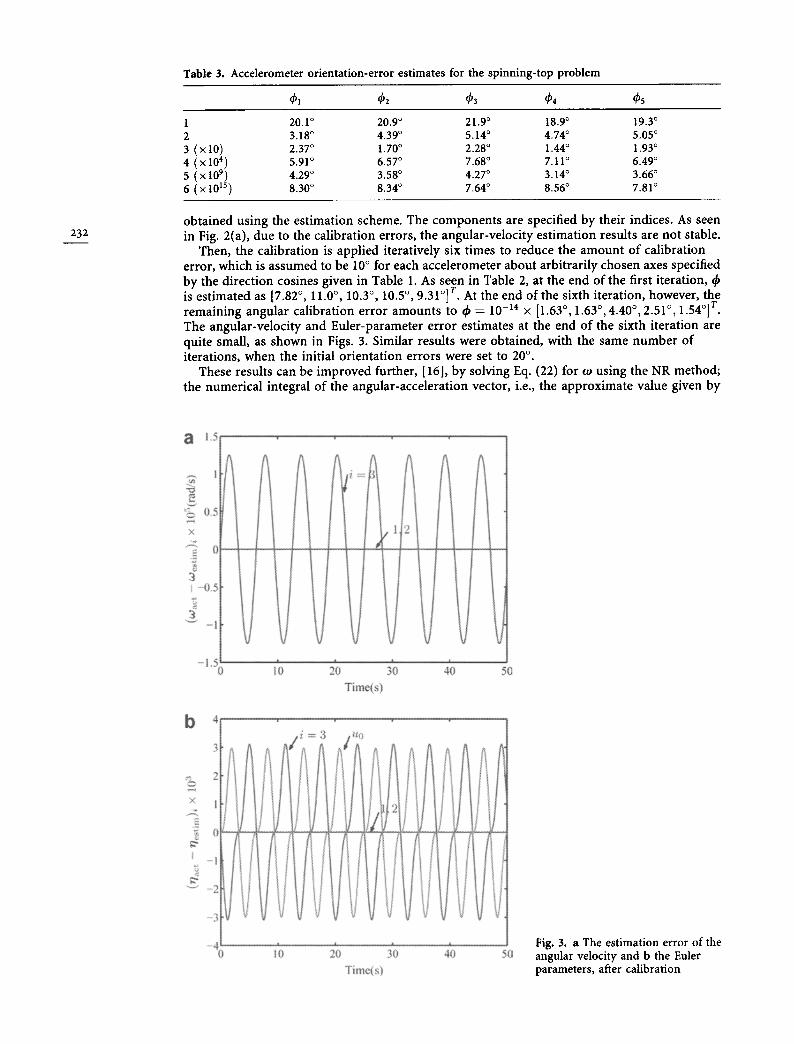
Table 3. Accelerometer orientation-error estimates for the spinning-top problem

1 20.1 ~ 20.9 ~ 21.9 ~ 18.9 ~ 19.3 ~ 2 3.18 ~ 4.39 ~ 5.14 ~ 4.74 ~ 5.05 ~ 3 ( x 10) 2.37 ~ 1.70 ~ 2.28 ~ 1.44 ~ 1.93 ~ 4 (x 104) 5.91 ~ 6.57 ~ 7.68 ~ 7.11 ~ 6.49 ~ 5 ( x 109) 4.29 ~ 3.58 ~ 4.27 ~ 3.14 ~ 3.66 ~ 6 ( x 1015) 8.30 ~ 8.34 ~ 7.64 ~ 8.56 ~ 7.81 ~

232 ob ta ined us ing the es t ima t ion scheme. The c o m p o n e n t s are specif ied by their indices . As seen in Fig. 2(a), due to the ca l ib ra t ion errors , the angula r -ve loc i ty e s t ima t ion resul ts are not stable.

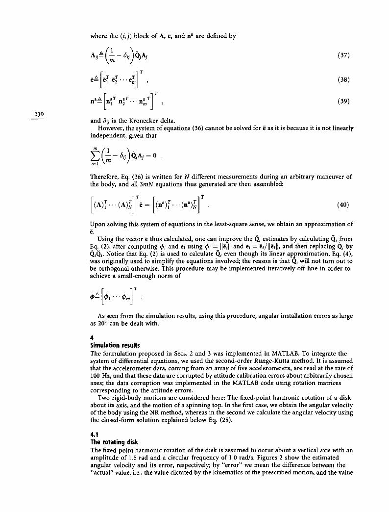
Then, the ca l ibra t ion is app l i ed i tera t ively six t imes to reduce the a m o u n t o f ca l ibra t ion error , which is a s sumed to be 10 ~ for each acce le romete r abou t a rb i t ra r i ly chosen axes specif ied by the d i rec t ion cosines given in Table 1. As seen in Table 2, at the end of the first i te ra t ion , is e s t ima ted as [7.82 ~ 11.0 ~ 10.3 ~ 10.5 ~ 9.31~ T. At the end of the sixth i te ra t ion , however , the r ema in ing angu la r ca l ibra t ion e r ro r amoun t s to ~b = 10 -14 • [1.63 ~ 1.63 ~ 4.40 ~ 2.51 ~ 1.54~ r. The angula r -ve loc i ty and Eu le r -pa ramete r e r ro r es t imates at the end o f the s ixth i te ra t ion are qui te small , as shown in Figs. 3. Similar resul ts were ob ta ined , wi th the same n u m b e r of i tera t ions , when the ini t ial o r i en ta t ion e r rors were set to 20 ~ .

These resul ts can be i m p r o v e d further , [16], b y solving Eq. (22) for to using the NR method; the numer ica l in tegral o f the angu la r -acce le ra t ion vector, i.e., the a p p r o x i m a t e value given by

a t,5

~ 0,.5

X

!4 -0-5

~ ' - I

-1.5

T r T 1"

10 20 30 40 50 Time(s)

4i . . . . ! ! / ~=3 l,,o /

0 t0 20 30 40 50 Time(s)

Fig. 3. a The estimation error of the angular velocity and b the Euler parameters, after calibration

a t.5

~ 0.5

~ ,.,-0, 5

-!,5 10 20 30 40 50

Time(s)

b 5t. ~- r T v a

'f/I II II I111 II tt fl/t/I If/t/1/I/l t17 -'~

~',-~0 ~ Fig. 4. a The estimation error of - 0 10 20 30 40 50 skew-symmetric v ~ and b that of

Time(s) the Euler parameters

Eq. (26), provides the required initial guess. Figures 4 show the errors after applying the Newton-Raphson scheme with a relative tolerance of 10 -7. One interesting point in Fig. 4(a) is that, as opposed to Fig. 3(a), the errors are the largest when the angular velocity undergoes a sign change, the sole reason being the inherent sign indeterminacy of the square-root problem. The angular-velocity results obtained at this stage are by three orders of magnitude more accurate than the results reported in [15]. As for the quaternion errors, the results shown in Fig. 4(b) are at least as accurate, without resorting to an additional sensor.

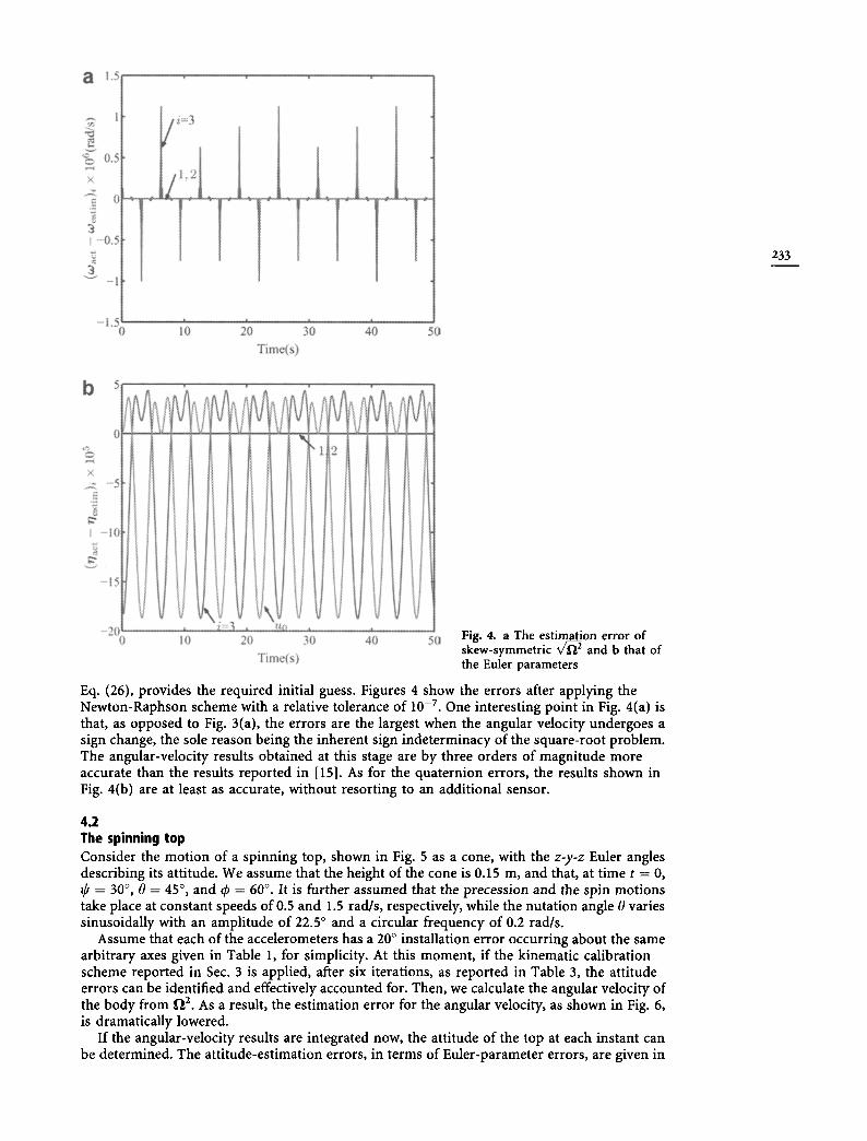
4.2 The spinning top Consider the motion of a spinning top, shown in Fig. 5 as a cone, with the z-y-z Euler angles describing its attitude. We assume that the height of the cone is 0.15 m, and that, at time t = 0, ~b = 30 ~ 0 = 45 ~ and ~b = 60 ~ It is further assumed that the precession and the spin motions take place at constant speeds of 0.5 and 1.5 rad/s, respectively, while the nutation angle 0 varies sinusoidally with an amplitude of 22.5 ~ and a circular frequency of 0.2 rad/s.

Assume that each of the accelerometers has a 20 ~ installation error occurring about the same arbitrary axes given in Table 1, for simplicity. At this moment, if the kinematic calibration scheme reported in Sec. 3 is applied, after six iterations, as reported in Table 3, the attitude errors can be identified and effectively accounted for. Then, we calculate the angular velocity of the body from f12. As a result, the estimation error for the angular velocity, as shown in Fig. 6, is dramatically lowered.

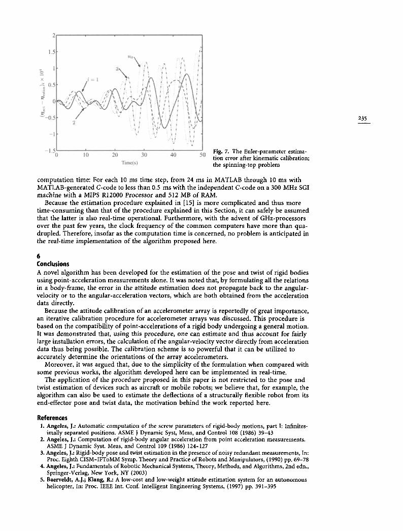
If the angular-velocity results are integrated now, the attitude of the top at each instant can be determined. The attitude-estimation errors, in terms of Euler-parameter errors, are given in

233

234

Z , ~1

0

? Yl

2~

X2

Y

X

~L" 1

X Fig. 5. A spinning top

-0.5 x

E

3 -1 I

- 1.5

I 3 I

I I I I I t 2

t i = l

W ~ m

20 10 20 30 40 50 Time(s)

Fig. 6. Error in calculating to after kinematic calibration; the spinning- top problem

Fig. 7. As seen from this figure, the error is increasing; this was actually expected, for the integration operation is inherently unstable.

5 R e a l - t i m e o p e r a t i o n

As explained in [15], in order to render the formulation real-time operational, the authors "translated" the MATLAB m-files into C-code, and subsequently compiled the code thus generated using MATLAB's m c c translator. Even though special attention was paid to the minimization of the number of calculations in MATLAB, simulations revealed that the m c c -

generated C-code was not fast enough. Therefore, an independent estimation program was developed in C. As reported in that paper, the simulations showed a dramatic improvement in

2

1,5 i~:~ \ ,.. ~ :i:!i x t.: i, i i

• / ; , t \ . . . . i \ 1

! o :

i " - ; ; i ' + ' - ' : . i : ~ It,: / j ~ I t / t

- i , !!'.v ! - r . . : . . . .

.... I 20 30 40 50 Time(s)

Fig. 7. The Euler-parameter estima- tion error after kinematic calibration; the spinning-top problem

235

computation time: For each 10 ms time step, from 24 ms in MATLAB through 10 ms with MATLAB-generated C-code to less than 0.5 ms with the independent C-code on a 300 MHz SGI machine with a MIPS R12000 Processor and 512 MB of RAM.

Because the estimation procedure explained in [15] is more complicated and thus more time-consuming than that of the procedure explained in this Section, it can safely be assumed that the latter is also real-time operational. Furthermore, with the advent of GHz-processors over the past few years, the clock frequency of the common computers have more than qua- drupled. Therefore, insofar as the computation time is concerned, no problem is anticipated in the real-time implementation of the algorithm proposed here.

6 Conclusions A novel algorithm has been developed for the estimation of the pose and twist of rigid bodies using point-acceleration measurements alone. It was noted that, by formulating all the relations in a body-frame, the error in the attitude estimation does not propagate back to the angular- velocity or to the angular-acceleration vectors, which are both obtained from the acceleration data directly.

Because the attitude calibration of an accelerometer array is reportedly of great importance, an iterative calibration procedure for accelerometer arrays was discussed. This procedure is based on the compatibility of point-accelerations of a rigid body undergoing a general motion. It was demonstrated that, using this procedure, one can estimate and thus account for fairly large installation errors, the calculation of the angular-velocity vector directly from acceleration data thus being possible. The calibration scheme is so powerful that it can be utilized to accurately determine the orientations of the array accelerometers.

Moreover, it was argued that, due to the simplicity of the formulation when compared with some previous works, the algorithm developed here can be implemented in real-time.

The application of the procedure proposed in this paper is not restricted to the pose and twist estimation of devices such as aircraft or mobile robots; we believe that, for example, the algorithm can also be used to estimate the deflections of a structurally flexible robot from its end-effector pose and twist data, the motivation behind the work reported here.

References 1. Angeles, I.: Automatic computation of the screw parameters of rigid-body motions, part I: Infinites-

imally separated positions. ASME I Dynamic Syst, Meas, and Control 108 (1986) 39-43 2. Angeles, 1.: Computation of rigid-body angular acceleration from point acceleration measurements.

ASME ] Dynamic Syst. Meas, and Control 109 (1986) 124-127 3. Angeles, l.: Rigid-body pose and twist estimation in the presence of noisy redundant measurements, In:

Proc. Eighth CISM-IFToMM Symp. Theory and Practice of Robots and Manipulators, (1990) pp. 69-78 4. Angeles, 1.: Fundamentals of Robotic Mechanical Systems, Theory, Methods, and Algorithms, 2nd edn.,

Springer-Vedag, New York, NY (2003) 5. Baerveldt, A.I.; Klang, R.: A low-cost and low-weight attitude estimation system for an autonomous

helicopter, In: Proc. IEEE Int. Conf. Intelligent Engineering Systems, (1997) pp. 391-395

236

6. Chen, J.H.; Lee, S.C.; De Bra, D.B.: Gyroscope fee strapdown inertial measurement unit by six linear accelerometers. AIAA J of Guidance, Control, and Dynamics 17 (1994) 286-290

7. Giardina, C.IL; Bronson, R.; Wallen, L.: An optimal normalization scheme. IEEE Trans Aerospace and Electronic Systems 11 (1975) 443-446

8. Goldstein, H.: Classical Mechanics, 2nd edn., Addison-Wesley, Reading, MA (1980) 9. Grubin, C.: Attitude determination for a strapdown inertial system using the euler axis/angle and

quaternion parameters, In: AIAA (1973) paper 73-900, Key Biscayne, FL 10. Markeley, F.L.; Berman, N.; Shaked, U.: Deterministic EKF-like estimator for spacecraft attitude

estimation, In: Proc. American Control Conference, (1994) pp. 247-251 11. Mital, N.K.; King, A.I.: Computation of rigid-body rotation in three-dimensional space from body-fixed

linear acceleration. ASME J of Appl Mech 46 (1979) 925-930 12. Mostov, K.S.; Soloviev, A.A.; John Koo, T.K.: Accelerometer based gyro-free multi-sensor generic

inertial device for automotive applications, In: IEEE Conf. Intelligent Transportation Systems, (1998) pp. 1047-1052

13. Padagonakar, A.J.; Krieger, K.W.; King, A.I.: Measurement of angular acceleration of a rigid body using linear accelerometers. ASME J of Appl Mech (1975) : 552-556

14. Parsa, K.: Dynamics, state estimation, and control of manipulators with rigid and flexible subsystems. Ph.D. thesis, McGill University, Montreal, Canada (2003)

15. Parsa, K.; Angeles, J.; Misra, A.K.: Pose and twist estimation of a rigid body using accelerometers, In: Proc. IEEE Int. Conf. Robotics and Automation, (2001) pp. 2873-2878

16. Parsa, K.; Angeles, J.; Misra, A.K.: Attitude calibration of an accelerometer array, In: Proc. IEEE Int. Conf. Robotics and Automation on CD Rom (2002)

17. Roumeliotis, S.L; Sukhatme, G.S.; Bekey, G.A.: Smoother based 3-D attitude estimaton for mobile robot localization, Tech. Rep. IRIS-98-363, USC, h t t p : / / i r i s .usc. edu / , .~ i r i s l i b / (1998)

18. Roumeliotis, S.I.; Sukhatme, G.S.; Bekey, G.A.: Circumventing dynamic modelling: Evaluation of the error-state Kalman fluter applied to mobile-robot localization, In: Proc. IEEE Int. Conf. Robotics and Automation, (1999) pp. 1656-1663

19. Sommer Ill, H.J.: Determination of first and second order instant screw parameters from landmark trajectories. ASME ] Mechanical Design 114 (1992) 274-282

20. Tan, C.W.; Park, S.; Mostov, K.; Varaiya, P.: Design of gyroscope-free navigation systems. In: IEEE Intelligent Systems Conference, (2001) pp. 286-291

21. Vaganay, l.; Aldon, M.J.; Fournier, A.: Mobile robot attitude estimation by fusion of inertial data, In: Proc. IEEE Int. Conf. Robotics and Automation, (1993) pp. 277-282

22. Wertz, J.R.: Spacecraft attitude determination and control 73 of Astrophysics and Space Science Library, D. Reidel Publishing Company, Dordrecht (1978)