Riemann Normal Coordinate expansions using Cadabra

Preprint: arXiv:0903.2087

Journal: Class.Quantum.Grav. 26 175017 (2009)

Riemann Normal Coordinate expansions

using Cadabra

Leo Brewin

School of Mathematical SciencesMonash University, 3800

Australia

12-Aug-2009

Abstract

We present the results of using the computer algebra program Cadabrato develop Riemann normal coordinate expansions of the metric andother geometrical quantities, in particular the geodesic arc-length. Allof the results are given to sixth-order in the curvature tensor.

1 Introduction

In a previous paper [1] we demonstrated, through a series of simple exam-ples, how a new computer algebra program, Cadabra ([2], [3], [4], [5]) couldbe employed to do the kinds of tensor computations often encountered inGeneral Relativity. The examples were deliberately chosen to be simple. Soit is reasonable to wonder how Cadabra might handle much more challengingcomputations. To explore this question we put Cadabra to the task of com-puting the Riemann normal coordinate expansions of the metric and othergeometrical quantities, in particular the geodesic arc length. Such computa-tions are known to be, at higher orders, very demanding and prohibitivelydifficult to compute by hand. Here we will show that Cadabra handles thesecomputations with ease.

There is also a direct practical purpose to these calculations. We are devel-oping ([6], [7]) an approach to numerical relativity that uses a lattice, similarto that used in the Regge calculus ([8], [9], [10]), as a way to record the

1

metric (through the table of leg-lengths) and topology (through the connec-tions between vertices) of the spacetime. Central to that approach is theuse of Riemann normal coordinates in the computation of the Riemann cur-vatures given just the leg-lengths and (some) angles. For this to work weneed an equation that links the curvatures to the geodesic arc-length (theleg-lengths). The result is equation (11.21) in section (11).

The basic idea behind Riemann normal coordinates is to use the geodesicsthrough a given point to define the coordinates for nearby points. Let thegiven point be O (this will be the origin of the Riemann normal frame) andconsider some nearby point P . If P is sufficiently close to O then there existsa unique geodesic joining O to P . Let va be the components of the unittangent vector to this geodesic at O and let s be the geodesic arc lengthmeasured from O to P . Then the Riemann normal coordinates of P relativeto O are defined to be xa = sva. These coordinates are well defined providedthe geodesics do not cross (which we can always ensure by choosing theneighbourhood of O to be sufficiently small).

One trivial consequence of this definition is that all geodesics through O areof the form xa(s) = sva and that the va are constant along each geodesic.This implies, by direct substitution into the geodesic equation, that Γcab = 0at O which in turn implies that gab,c = 0 at O. Suppose now that we wereto expand the metric as a Taylor series in xa about O. In that series therewould only be the zero, second and higher derivatives of the gab. Thus theleading terms of the metric could be expressed as a sum of a constant partplus a curvature part. If the curvature is weak this can be interpreted asan expansion of the metric in powers (and derivatives) of the curvature.Likewise one can imagine similar expansions of other geometrical quantities(e.g. geodesics, arc length) in terms of a flat space part plus a curvaturecontribution.

Higher order expansions are extremely tedious to compute by hand. Somehardy souls ([11], [12], [13]) have endured the journey (Muller et al ([14])venture as far as 11-th order expansions for the metric (i.e. to terms involvingthe 8-th derivative of the curvatures, the notion of order will be defined inthe following section). However most people settle for just the first two non-trivial curvature terms (i.e. R and ∇R).

As we will see, the easiest expansion to compute is that for the metric inpowers of the curvatures and its derivatives. Much more challenging is theexpression that allows the Riemann normal coordinates to be constructedfrom a given set of coordinates. This later calculation involves the solutionof a two point boundary value problem – not a job for the faint-hearted.

2

The expansion of the metric in Riemann normal form can be found in manyarticles. For those with a mathematical bent see ([15], [16], [17]) and inparticular the elegant exposition by Gray ([18], [19]). For applications inphysics see ([20], [21], [22]).

2 Conformal coordinates

Each algorithm given later in this paper yields polynomial approximationsto particular geometric quantities (e.g. the metric). Higher order approxi-mations are obtained by recursive application of the algorithms.

In this section we will define what we mean when we say that the polynomialSε is an expansion of S up to and including terms of order O (εn). We willdo so by introducing a conformal transformation of the original metric.

Consider some neighbourhood of O and let ε be a typical length scale forO (for example, ε might be the length of the largest geodesic that passesthrough O and confined by the neighbourhood). Construct any regular setof coordinates xa (i.e. such that the metric components are non-singular) inthe neighbourhood of O and let the coordinates of O be xa?. We will use theword patch to denote the neighbourhood of O in which these coordinates aredefined. Now define a new set of coordinates ya by

xa = xa? + εya

and thusds2 = gab(x)dxadxb = ε2gab(x? + εy)dyadyb

Now define the conformal metric ds by ds = ds/ε2. This leads to

ds2 = gab(x? + εy)dyadyb = gab(y, ε)dyadyb

andgab = gab , gab,c = εgab,c , gab,cd = ε2gab,cd at O

where the partial derivatives on the left are with respect to y and those onthe right are with respect to x. Since gab(x?) does not depend on ε we havethe general result that

gab,i1i2i3···in = O (εn) at O

3

From this it follows, by simple inspection of the standard equations, that

Γabc,i1i2i3···in = O(εn+1

)at O

Rabcd,i1i2i3···in = O

(εn+2

)at O

There are now two ways to look at the patch. We can view it as patch oflength scale ε with a curvature independent of ε. Or we can view it as patchof fixed size but with a curvature that depends on ε (and where the limitε → 0 corresponds to flat space). This later view is useful since in using itwe can be sure that the series expansions around flat space are convergent(for a sufficiently small ε).

We will use these conformal coordinates for the remainder of this paper. Asthere is no longer any reason to distinguish between xa and ya we replaceya with xa. The xa will now be treated as generic coordinates (but keep inmind that we are working in a conformal gauge).

Finally, when we say that Sε is an expansion of S up to and including termsof order O (εn) we mean that

0 < limε→0

|S − Sε|εn+1

< M

for some finite positive M i.e. if S were expanded as a Taylor series in εaround ε = 0 then S and Sε would differ by terms proportional to εn+1.

3 Riemann Normal Coordinates

Suppose, as is almost always the case, that our coordinates xa are not inRiemann normal form. How might we transform to a local set of Riemannnormal coordinates? If we were to appeal to the simple definition ya =sva we would soon encounter a hurdle. The quantities va are rarely knownexplicitly but must instead be computed by solving a two-point boundaryvalue problem. This is non-trivial but it can be dealt with in stages. Firstconstruct a Taylor series expansion for an arbitrary geodesic passing throughO. This solution to the initial value problem will depend on two integrationconstants, xa and xa, being the respective values of xa(s) and dxa/ds at s = 0.Next use a fixed-point iterative scheme to produce successive approximationsto xa so that the geodesic passes through both points O and P . Then finallycompute va as dxa/ds at s = 0. This is exactly the plan which we will follow.

4

It is well known that Riemann normal coordinates can always be constructedlocally around any non singular point (see [19]). Thus we will not concernourselves here with issues such as existence and convergence but rather wewill focus our attention on developing algorithms for expressing various quan-tities in Riemann normal form.

3.1 The initial value problem

Our aim here is to obtain a Taylor series, about the point O, for solution ofthe geodesic equation

0 =d2xa

ds2+ Γabc(x)

dxb

ds

dxc

ds

subject to the initial conditions xa(s) = xa and dxa/ds = xa at s = 0.

We choose s = 0 at O and we write the Taylor series for xa(s) as

xa(s) = xa|s=0 + sdxa

ds

∣∣∣∣s=0

+∞∑n=2

sn

n!

dnxa

dsn

∣∣∣∣s=0

The second and higher derivatives can be obtained by successive differentia-tion of the geodesic equation leading to

xa(s) = xa + sxa −∞∑n=2

sn

n!Γai1i2i3···inx

i1xi2xi3 · · · xin (3.1)

where the Γai1i2i3···in , known as generalised connections, are defined recur-sively by

Γai1i2i3···in = Γa(i1i2i3···in−1,in) − nΓap(i2i3···in−1Γpi1in) (3.2)

Note that the use of round brackets (...) denotes total symmetrisation overthe included indices (see Appendix A for more details).

A convenient shorthand for equation (3.2) in terms of covariant derivativescan be obtained if you ignore (in this context alone) the single upper index.This leads to the compact notation

Γai1i2i3···in = Γa(i1i2;i3i4i5···in) (3.3)

5

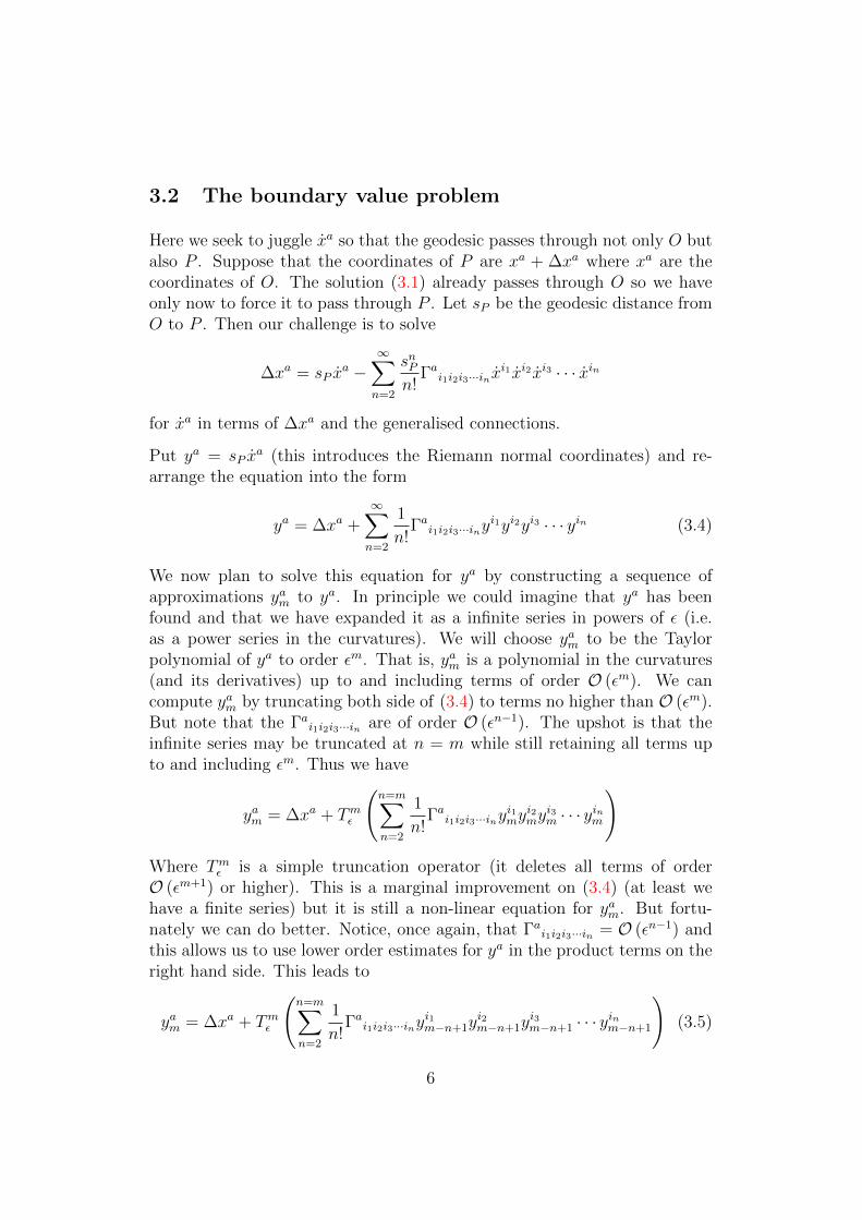
3.2 The boundary value problem

Here we seek to juggle xa so that the geodesic passes through not only O butalso P . Suppose that the coordinates of P are xa + ∆xa where xa are thecoordinates of O. The solution (3.1) already passes through O so we haveonly now to force it to pass through P . Let sP be the geodesic distance fromO to P . Then our challenge is to solve

∆xa = sP xa −

∞∑n=2

snPn!

Γai1i2i3···inxi1xi2xi3 · · · xin

for xa in terms of ∆xa and the generalised connections.

Put ya = sP xa (this introduces the Riemann normal coordinates) and re-

arrange the equation into the form

ya = ∆xa +∞∑n=2

1

n!Γai1i2i3···iny

i1yi2yi3 · · · yin (3.4)

We now plan to solve this equation for ya by constructing a sequence ofapproximations yam to ya. In principle we could imagine that ya has beenfound and that we have expanded it as a infinite series in powers of ε (i.e.as a power series in the curvatures). We will choose yam to be the Taylorpolynomial of ya to order εm. That is, yam is a polynomial in the curvatures(and its derivatives) up to and including terms of order O (εm). We cancompute yam by truncating both side of (3.4) to terms no higher than O (εm).But note that the Γai1i2i3···in are of order O (εn−1). The upshot is that theinfinite series may be truncated at n = m while still retaining all terms upto and including εm. Thus we have

yam = ∆xa + Tmε

(n=m∑n=2

1

n!Γai1i2i3···iny

i1my

i2my

i3m · · · yinm

)

Where Tmε is a simple truncation operator (it deletes all terms of orderO (εm+1) or higher). This is a marginal improvement on (3.4) (at least wehave a finite series) but it is still a non-linear equation for yam. But fortu-nately we can do better. Notice, once again, that Γai1i2i3···in = O (εn−1) andthis allows us to use lower order estimates for ya in the product terms on theright hand side. This leads to

yam = ∆xa + Tmε

(n=m∑n=2

1

n!Γai1i2i3···iny

i1m−n+1y

i2m−n+1y

i3m−n+1 · · · yinm−n+1

)(3.5)

6

Now we see that yam appears only on the left hand side and thus we can usethis equation to recursively compute yap for p = 2, 3, 4, · · ·. Here are the firstfew yam. We start with the lowest order approximation,

ya0 = ∆xa

and as there are no ε1 terms in (3.4) we have

ya1 = ya0 = ∆xa

Now set m = 2 in equation (3.5) to obtain

ya2 = ∆xa + T 2ε

(1

2!Γai1i2y

i11 y

i21

)= ∆xa +

1

2Γai1i2∆x

i11 ∆xi21

and once more, with m = 3, with the result

ya3 = ∆xa + T 3ε

(1

2!Γai1i2y

i12 y

i22 +

1

3!Γai1i2i3y

i11 y

i21 y

i31

)= ∆xa +

1

2Γai1i2∆x

i1∆xi2 +1

6

(Γabi1Γ

bi2i3 + Γai1i2,i3

)∆xi1∆xi2∆xi3

This process may seem simple but looks can be deceiving – the higher orderyam contain a profusion of terms that, when computed by hand, are largelyunmanageable beyond m ≈ 7. We will return to this point later when wediscuss the use of Cadabra to perform these computations.

This completes our first objective – to find a way to transform from anynon-singular set of coordinates to a local set of Riemann normal coordinates.The question we now pose is – what form does the metric take in thesecoordinates? This is the subject of the second next section. But first weshall take a short moment to introduce some new notation.

4 Notation

The calculations we are undertaking are flooded with expression such as

Γai1i2i3···in+1 = Γa(i1i2i3···in,in+1) − (n+ 1)Γap(i2i3···inΓpi1in+1)

in which long stretches of indices like i1i2i3 · · · in abound. This is tedious towrite and, in the authors opinion, rather untidy. Here we propose a variation

7

on the notation that is both easy to read and write while not detracting fromthe meaning in the expression. The proposal is that a sequence of indicessuch as i1i2i3 · · · in be replaced with a single index of the form i. In thisnotation the previous equation could be written as

Γabcd = Γa(bc,d) − (n+ 1)Γap(cΓpbd)

where c contains n > 0 indices. In cases where the number of hidden indicesneeds to be made clear we will either say so in words (as we did in theprevious example) or we will include the number as a subscript, for example

Γabcnd = Γa(bcn,d) − (n+ 1)Γap(cnΓpbd)

This version is however, not as clean as the previous version.

For equations like

0 = Γabc,i1i2i3···inAi1Ai2Ai3 · · ·Ain

we will write0 = Γabc,dA

.d

We chose this notation of single dot in A.d because of its suggestive form(of multiplication of as many copies of A as required to exhaust the indiceswithin d). Here is another common construction(

· · ·((

Γabc,i1Ai1),i2Ai2),i3Ai3 · · ·

),in

Ain

How might we tidy this up? By including a dot before the derivative indexd, like this

Γabc,.dA.d

These simple changes bring some degree of normalcy to the printed form butthose gains rapidly pale into insignificance when we ask Cadabra (in section(11)) to display the results for the sixth order Riemann normal expansions.These results contain expressions with symmetries in some of the indiceswhich when printed can stretch over many A4-pages. The reason is in partthat the expressions are inherently long but also because Cadabra does notuse the round-bracket notation to denote symmetrisation over a set of indices.Instead it uses the fully expanded form which, on paper, can lead to an n!explosion in otherwise similar looking terms. We will try to minimise thisproblem as follows. Suppose we have an object Aabcde which we know tobe symmetric on the indices (cde). We create an arbitrary Ba and instruct

8

Cadabra to simplify the expression AabcdeBcBdBe as much as possible. Then

we set Ba equal to one just prior to printing the expression. But how do weconvey to the reader that this operation has been performed? The expressionthat we are trying to print will always be the right hand side of some equationsuch as Dabcde = Aab(cde) and thus Dabcde is also symmetric on (cde). Sowhen we print this equation we will include the round brackets on the lefthand side. Thus we would display the results as Dab(cde) = Aabcde and wewould understand that the right hand side should be symmetrised over (cde).Clearly this notational device should only ever be used at the end of thecalculations.

Our final notational device concerns cases where we want to exclude an indexfrom symmetrisation. The normal practise is to exclude an index by enclosingit in a pair of vertical lines. In our variation we will place a dot abovethe excluded index. Thus, where other authors might write (ab|c|d|e|fg) tosignify symmetrisation over only a, b, d, f and g, we will write (abcdefg).

Though these variations might appear to make only marginal improvementsin the printed equations they have made it considerably easier for the authorin creating the LaTeX code for this document.

5 The metric in Riemann normal form

In the preceding section we chose to distinguish between generic and Riemannnormal coordinates by using the symbols xa and ya respectively. We will now,for notational convenience and to accord with convention, revert to usingxa for the Riemann normal coordinates while stripping ya of any specialmeaning.

Our aim in this section is to express the metric in Riemann normal form.This will take the form of an infinite series in powers of the curvature tensorand its derivatives. We start by writing out the Taylor series for the metricaround xa = 0

gab(x) = gab +∞∑n=1

1

n!gab,c x

.c

where c contains n indices and gab are constants (e.g. gab = diag(1, 1, 1, · · ·)).

Our present task is to express the partial derivatives of the metric in termsof the Riemann tensor. From the standard definition of a metric compatibleconnection we have

gab,cd = (gaeΓebc + gebΓ

eac),d

9

and since gab,cd is totally symmetric in cd we also have

gab,cd =(gaeΓ

eb(c

),d) +

(gebΓ

ea(c

),d)

Two points should be noted, first, the connection appears only in the formΓab(c,d), second, the left hand side contains derivatives one order higher thanin the corresponding terms on the right hand side. The upshot is that we canuse this equation to recursively compute all of the metric derivatives solelyin terms of the Γab(c,d) and the constants gab. In this way we could expressthe above Taylor series for the metric in terms of the connection. But wecan go one stage further – the derivatives of the connection must surely tiein with the curvatures. Thus we are led to review the standard definition forthe curvature, which after a series of derivatives, can be written in the form

Ra(bcd,e) = Γad(bc,e) − Γa(bc,e)d +

(Γai(cΓ

ibd

),e) −

(ΓaidΓ

i(bc

),e)

(Please note that the Γadbc in Γad(bc,e) is the first of the generalised connectionsdiscussed earlier in section (3.1)). Can we use this to eliminate the connectionand its derivatives from the metric? Yes, but only after we specialise to theRiemann normal coordinates.

Recall that, in Riemann normal coordinates, all geodesics through O are ofthe form

xa(s) = sva

which upon substitution into the geodesic equations leads to

0 = Γa(bc) at O

It follows, by recursion on equation (3.3), that

0 = Γa(bc,d) at O (5.1)

We also know that Γabc,ed is separately symmetric in its first pair of indicesand in the remaining (n + 1) lower indices (assuming e contains n indices).Thus using equation (A.1) we have

0 = (n+ 3)Γa(bc,ed) = 2Γad(b,ce) + (n+ 1)Γa(bc,e)d

We can use this to eliminate the Γa(bc,e)d term in the previous equation forthe curvature. The result, after a minor shuffling of terms is

(n+ 3)Γad(b,ce) = (n+ 1)(Ra

(bcd,e) −(Γai(cΓ

ibd

),e) +

(ΓaidΓ

i(bc

),e)

)10

(the reason for rearranging the terms will become clear in a moment). Notealso that the last term in the previous equation can be eliminated by equation(5.1) and the product rule.

In summary, the equations of interest are

gab(x) = gab +∞∑n=1

1

n!gab,c x

.c (5.2)

gab,cd =(gaeΓ

eb(c

),d) +

(gebΓ

ea(c

),d) (5.3)

(n+ 3)Γad(b,ce) = (n+ 1)(Ra

(bcd,e) −(Γai(cΓ

ibd

),e)

)(5.4)

We use these equations as follows. First, equation (5.4) is used to recursivelycompute the Γab(c,ed) in terms of the Riemann tensor and its partial deriva-tives (this was the reason behind the shuffling of terms noted above). Notethat e in equation (5.4) contains n hidden indices. The Γab(c,d) are then sub-stituted into (5.3) which in turn is used to recursively express all of the gab,cin terms of the Riemann tensor and its partial derivatives. When the dustsettles we will have a finite series expansion for the metric in terms of theRiemann tensor and its partial derivatives. The result, accurate to O (ε4), is

gab (x) = gab −1

3xcxdRacbd −

1

6xcxdxe∂cRadbe +O

(ε4)

We conclude this section by introducing one final variation to the algorithmjust given – an option to re-express the metric in terms of the covariant ratherthan partial derivatives of the curvatures.

It is not hard to see that after a series of covariant derivatives one wouldobtain an equation of the form, in any coordinate frame,

Ra(bcd;e) = Ra

(bcd,e) +Qa(bcde)

where Qa(bcde) is a function of the Γabc, the Ra

bcd and their partial derivatives.If this is going to sit nicely with our algorithm given above then we will needto show, in the Riemann normal frame, that this equation only containsconnection terms of the form Γpq(r,s). Fortunately this is rather easy to do.

Each term of the form Γpqr,s in Q arose during one round of covariant dif-ferentiation. Thus at least one of the indices q, r and all of the indices ins must be drawn from the index list e. If both q and r are contained in ethen the term is of the form Γp(qr,s) and thus will vanish when we specialise

11

to the Riemann normal frame. This completes the proof. If we re-arrangethe above equation into the following form

Ra(bcd,e) = Ra

(bcd;e) −Qa(bcde) (5.5)

we can use it to recursively compute all of the partial derivatives of the cur-vatures in terms of their covariant derivatives. The Qa

(bcde) will contain lowerorder derivatives of the curvatures and partial derivatives of the connectionall of which can be eliminated (in favour of covariant derivatives) using previ-ously computed results. For the first two derivatives we find that the partialand covariant derivatives are equal but differences do appear in higher orderderivatives. More details will be given in a later section.

These calculations, as simple as they may appear, are exceedingly tedious todo except for the first few terms. The recursive nature of the calculationsrequires frequent substitution of one result into another which causes anexplosion in the number of terms that must be handled. Not only is thistedious but its is also extremely prone to human error. Calculations of thiskind are clearly best left to a computer. We shall return to this point lateron.

6 The inverse metric in Riemann normal form

Most of the hard work is now behind us and we can now develop algorithmsfor Riemann normal expansions for other interesting quantities, in this in-stance the inverse metric gab(x). In the previous section we used 0 = gab;c asour starting point. On this occasion we start with 0 = gab;c. Then, followinga path similar to that used in the previous section, we arrive at the followingequations

gab(x) = gab +∞∑n=1

1

n!gab,c x

.c (6.1)

gab,cd = −(gaeΓbe(c

),d) −

(gebΓae(c

),d) (6.2)

(n+ 3)Γad(b,ce) = (n+ 1)(Ra

(bcd,e) −(Γai(cΓ

ibd

),e)

)(5.4)

These equations can be used to construct the series expansion for gab(x),which to O (ε4) is

gab (x) = gab +1

3xcxdRa

cbd +

1

6xcxdxe∂cR

adbe +O

(ε4)

12

7 Generalised connections

In section (3.1) we saw that the generalised connections Γabcd arose fromsuccessive differentiation of the geodesic equation and that they can be com-puted recursively using

Γabcd = Γa(bc,d) − (n+ 1)Γap(cΓpbd) (3.2)

where the index list c contains n > 0 indices, or directly using

Γabcd = Γa(bc;d) (3.3)

Here are the first three generalised connections

Γa(bc)(x) = Γa bc

Γa(bcd)(x) = ∂bΓacd − 2 Γa beΓ

ecd

Γa(bcde)(x) = −Γf bc∂fΓade − 4 Γf bc∂dΓ

aef + ∂bcΓ

ade

+ 2 Γa fgΓfbcΓ

gde + 4 Γa bfΓ

fcgΓ

gde − 2 Γa bf∂cΓ

fde

and when we specialise to Riemann normal coordinates we obtain

Γa(bc)(x) =2

3xdRa

bdc +1

12xdxe (2∇bR

adec + 4∇dR

abec +∇aRdbec) +O

(ε4)

Γa(bcd)(x) =1

2xe∇bR

aced +O

(ε4)

Γa(bcde)(x) = O(ε4)

8 Geodesics

When first we spoke of Riemann normal coordinates we restricted our at-tention to the geodesics that passed through the point O. Now we wish tobe somewhat less restrictive. We would like to know how to construct anygeodesic in the neighbourhood of O. Here we will once again be buildingsolutions of the geodesic equations and as before we will consider two sepa-rate cases, first, the geodesic initial value problem and second, the geodesicboundary value problems.

Most of the machinery that we need to tackle these questions has alreadybeen developed. Here we apply the formalism developed in sections (3.1) and(3.2) to the metric in Riemann normal form as obtained in section (5).

13

8.1 Geodesic initial value problem

Consider a point P distinct from O. At P we can assume that the generalisedconnections do not vanish (which is generally true, the exception being flatspace). Thus the coordinates xa in the neighbourhood of P do not constitutea Riemann normal frame relative to P . But as P lies in the patch for O weknow that the metric is non-singular at P and thus we should be able toconstruct a new set of Riemann normal coordinates, ya, with P as the origin.

We have seen this problem once before, in section (3.2). Using equation (3.1)and the generalised connections from section (7) we find

xa (s) = xa + sxa − 1

24s2xbxc

(8xdRa

bdc + 2xdxe∇bRadec + 4xdxe∇dR

abec

+ xdxe∇aRdbec

)− 1

12s3xbxcxdxe∇bR

aced +O

(ε4)

8.2 Geodesic boundary value problem

Consider now the case where we have three distinct points O, P and Q. Inthis section we seek to compute the geodesic that passes through P and Q.We use the equation (3.5) of the generalised connections from section (7) toobtain

xa (λ) = xa + λxa1 + λ2xa2 + λ3xa3 +O(ε4)

xa1 = ∆x a +1

3xb∆x c∆x dRa

cbd +1

12xbxc∆x d∆x e∇dR

abce

+1

6xbxc∆x d∆x e∇bR

adce +

1

24xbxc∆x d∆x e∇aRbdce

+1

12xb∆x c∆x d∆x e∇cR

adbe

xa2 = −1

3xb∆x c∆x dRa

cbd −1

12xbxc∆x d∆x e∇dR

abce

− 1

6xbxc∆x d∆x e∇bR

adce −

1

24xbxc∆x d∆x e∇aRbdce

xa3 =

(−1

12

)xb∆x c∆x d∆x e∇cR

adbe

where λ = s/LPQ is the scaled geodesic distance from P (λ = 0) to Q(λ = 1).

14

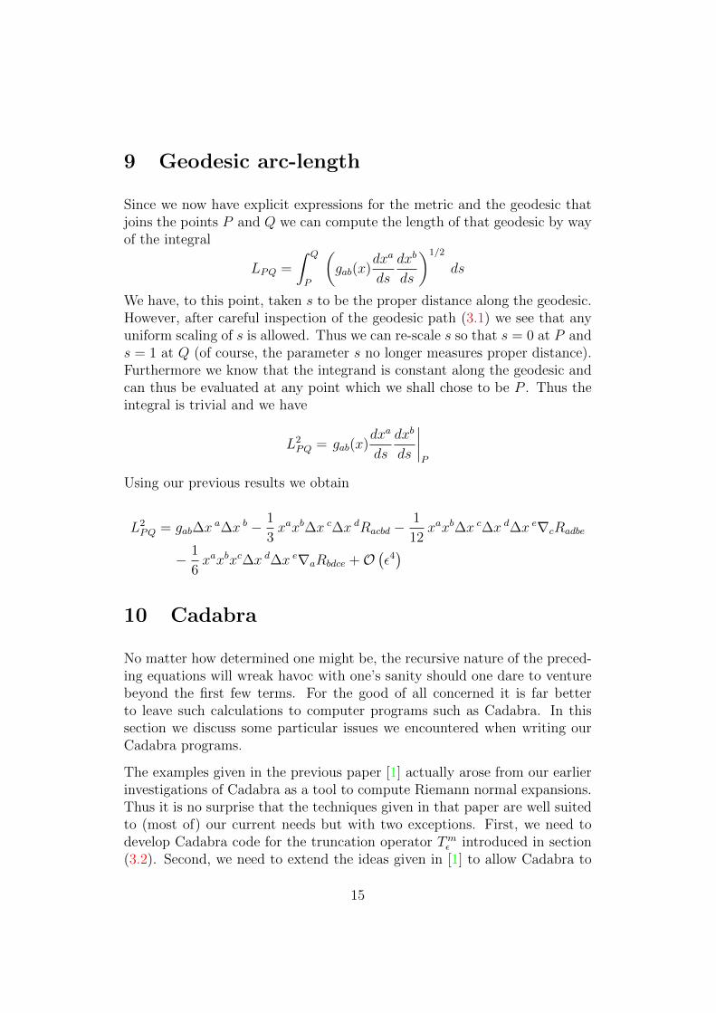
9 Geodesic arc-length

Since we now have explicit expressions for the metric and the geodesic thatjoins the points P and Q we can compute the length of that geodesic by wayof the integral

LPQ =

∫ Q

P

(gab(x)

dxa

ds

dxb

ds

)1/2

ds

We have, to this point, taken s to be the proper distance along the geodesic.However, after careful inspection of the geodesic path (3.1) we see that anyuniform scaling of s is allowed. Thus we can re-scale s so that s = 0 at P ands = 1 at Q (of course, the parameter s no longer measures proper distance).Furthermore we know that the integrand is constant along the geodesic andcan thus be evaluated at any point which we shall chose to be P . Thus theintegral is trivial and we have

L2PQ = gab(x)

dxa

ds

dxb

ds

∣∣∣∣P

Using our previous results we obtain

L2PQ = gab∆x

a∆x b − 1

3xaxb∆x c∆x dRacbd −

1

12xaxb∆x c∆x d∆x e∇cRadbe

− 1

6xaxbxc∆x d∆x e∇aRbdce +O

(ε4)

10 Cadabra

No matter how determined one might be, the recursive nature of the preced-ing equations will wreak havoc with one’s sanity should one dare to venturebeyond the first few terms. For the good of all concerned it is far betterto leave such calculations to computer programs such as Cadabra. In thissection we discuss some particular issues we encountered when writing ourCadabra programs.

The examples given in the previous paper [1] actually arose from our earlierinvestigations of Cadabra as a tool to compute Riemann normal expansions.Thus it is no surprise that the techniques given in that paper are well suitedto (most of) our current needs but with two exceptions. First, we need todevelop Cadabra code for the truncation operator Tmε introduced in section(3.2). Second, we need to extend the ideas given in [1] to allow Cadabra to

15

compute the symmetrised derivatives of arbitrary tensors, such as Rab(cd;e).

We shall deal with these issues in the following sections after which we willpresent the final Cadabra generated expressions (to O (ε6) and in all theirgory detail).

10.1 Truncation of polynomials

In section (3.2) we introduced a truncation operator Tmε . Here we discusshow we constructed that operator in our Cadabra code. It happens to bean extremely useful piece of code and is used extensively throughout ourCadabra code.

Suppose you are asked to extract the leading terms from an expression suchas

P a(x) = ca + cabxb + cabcx

bxc + cabcdxbxcxd

A standard approach would be to compute the derivatives of P a(x) at x =0. This approach would be rather simple to code in Cadabra. However aminor issue does pop up. Unless otherwise told, Cadabra will assume thatall objects have non-zero derivatives. Thus if Cadabra were instructed tocompute d/ds of the above expression it would dutifully do so but it wouldtreat the x’s and the coefficients cab as possibly depending on s. Cadabra canbe coaxed to restrict the derivative operators to act only on specific objectsby using the ::Depends property and the @unwrap algorithm.

A better solution, one that does not involve derivatives, is to use Cadabra’s::Weight property and the @keep_weight algorithm. The idea is to assignweights to nominated objects (through the ::Weight property) and thenextract terms matching a chosen weight (using the @keep_weight algorithm).Here is a small piece of Cadabra code that does the job.

x^{a}::Weight(label=xterms,value=1).

poly:= c^{a}

+ c^{a}_{b} x^{b}

+ c^{a}_{b c} x^{b} x^{c}

+ c^{a}_{b c d} x^{b} x^{c} x^{d};

term00:=@(poly): @keep_weight!(term00){xterms}{0};

term01:=@(poly): @keep_weight!(term01){xterms}{1};

term02:=@(poly): @keep_weight!(term02){xterms}{2};

16

The first line identifies the xa terms as our target (which we name as xtermsso that they can be distinguished from other targets decalared by other in-stances of ::Weight). The next three lines then extract the 0th, 1st and2nd terms in the expression poly. The result would be exactly as if we hadwritten

term00:=c^{a};

term01:=c^{a}_{b} x^{b};

term02:=c^{a}_{b c} x^{b} x^{c};

The truncated polynomial (in this case a quadratic) could then be computedsimply as @(term00)+@(term01)+@(term02).

10.2 Symmetrised covariant derivatives

Let va be a tensor field and suppose we wish to compute va;b at the originof the Riemann normal frame, O. Construct any geodesic through P and anauxiliary field Aa throughout the patch containing O. Let the geodesic beparametrised by the proper distance s and described by xa = xa(s) with unittangent vector Da = dxa/ds. We choose Aa so that it is auto-parallel alongthe geodesic. Thus we have

dvads

= va,bDb

0 = ∇D Da =

dDa

ds+ ΓabcD

bDc

0 = ∇D Aa =

dAa

ds+ ΓabcA

bDc

from which it follows that

va;bAaDb =

dn(vaAa)

dsnat O

where b contains n indices. Thus any higher order covariant derivative canbe obtained simply by expanding the right hand side, one derivative at atime, while using the parallel transport conditions listed above to eliminatederivatives in Aa and Da. The Cadabra code for this is much the same. Eachsuccessive covariant derivative is obtained by applying d/ds to the previousresult then using substitutions to eliminate the newly introduced derivativesof Aa and Da. Comparing coefficients of AaDb across the equals sign willthen reveal an expression for va(;b), the fully symetrised covariant derivativeof va at O.

17

Note that 0 = Γa(bc,d) at O in Riemann normal coordinates and thus 0 =dnDa/dsn. This can be used to considerably simplify the above computa-tions.

This idea can be easily extended to other cases. For example, suppose werequire vab(c;de) at O. In this case we would introduce two auxiliary fields,Aa and Ba, each constrained to be auto-parallel along the chosen geodesic.Then following the above procedure we obtain

vab(c;de)AaBbDcDdDe =

d2(vabcAaBbDc)

ds2at O

10.3 Symmetrised derivatives of the Riemann tensor

By inspection of equation (5.4) we see that the only derivatives of the Rie-mann tensor that enter our calculations are of the form Ra

(bcd,e) and Ra(bcd;e).

According to the prescription given above we can compute the covariantderivatives in terms of the partial derivatives by the following procedure.

0 = ∇D Da =

dDa

ds

0 = ∇D Bab =

dBab

ds+ ΓadcB

dbD

c − ΓdbcBadD

c

Ra(bcd;e)B

caD

bDdDe =dn

dsn(Ra

bcdBcaD

bDd)

This is not exactly what we want – it yields the covariant derivatives in termsof the partial derivatives. We need instead, the partial derivatives expressedin terms of the covariant derivatives. In section (5) we provided one solutionto this problem. There we argued that the equations could be re-written inthe form

Ra(bcd,e) = Ra

(bcd;e) −Qa(bcde) (5.5)

where Qa(bcde) contains all the lower order symmetrised partial derivatives of

Rabcd. This algorithm certainly works but it is computationally expensive. If

for the moment we label the equation for the n-th derivative as En then ouralgorithm entails a whole hierarchy of substitutions of Ej into Ek for j < k.For example, to compute E4 we need to substitute E1 into E2, then E1 andE2 into E3, and finally, E1, E2 and E3 into E4. Our code took about 4 secondsto compute the first four derivatives but with one extra derivative this timegrew to 11 minutes. We did not bother to compute the sixth derivative (infact for the results given here we only need the first three derivatives).

18

It seems reasonable to ask : is there a better way? Indeed there is and thechanges required are very simple.

The auxiliary field Bab can be freely chosen so there is nothing stopping us

from setting Bab to be constant throughout the neighbourhood of O. Thus

every partial derivative of Bab is zero at O. What use is this to us? Consider

the equation (Ra

bcdBcaD

bDd);eD

e =dn

dsn(Ra

bcdBcaD

bDd)

This is clearly true for any Bab and Da = dxa/ds (and in any coordi-

nate frame). In our Riemann normal frame we have 0 = dnDa/dsn andwe have chosen 0 = Ba

c,e. Thus the right hand side can be reduced toRa

bcd,eBcaD

bDdDe. This leads to the following modified scheme (after swap-ping the left and right hand sides)

0 = Da;bD

b =dDa

ds

∇D Bab = Ba

b;cDc = ΓadcB

dbD

c − ΓdbcBadD

c

Rabcd,eB

caD

bDdDe = (RabcdB

ca) ;eD

bDdDe

This algorithm computes all the partial derivatives directly, without requiringany substitutions from previous results. It took less than 10 seconds tocompute the first five derivatives which is a dramatic improvement over ourprevious algorithm (11 minutes).

In our Cadabra code we compute all of the symmetrised partial derivatives(using the above algorithm) before we compute the metric expansion (equa-tions (5.2, 5.3, 5.4)). In this way we obtain a series expansions for the metricin terms of the covariant derivatives of the curvatures.

11 Expansions to sixth order

All of our O (ε6) Cadabra programs were not overly demanding on compu-tational resources, taking less than 2 minutes to run (on a MacOSX with anIntel cpu) and requiring less than 13 Mbyte of memory.

The Cadabra codes and several support scripts are available from the author’sweb site http://users.monash.edu.au/~leo.

19

Some of the following expansions can be compared directly with results ob-tained by traditional methods. In particular our expansions for the metricand its inverse, equations (11.1) and (11.2) agree exactly with those given inequations (17) and (18) respectively of [11]. Also, our equation (11.3) agreeswith that given in equation (A12) of [20].

The metric

180gab (x) = 180 gab−60xcxdRacbd−30xcxdxe∇cRadbe+8xcxdxexfRacgdRbegf

− 9xcxdxexf∇cdRaebf + 4xcxdxexfxgRachd∇eRbfhg

+ 4xcxdxexfxgRbchd∇eRafhg − 2xcxdxexfxg∇cdeRafbg +O(ε6)

(11.1)

The inverse metric

180gab (x) = 180 gab + 60xcxdRacbd + 30xcxdxe∇cR

adbe

+ 12xcxdxexfRacdgR

befg + 9xcxdxexf∇cdR

aebf

+ 6xcxdxexfxgRacdh∇eR

bfgh + 6xcxdxexfxgRb

cdh∇eRafgh

+ 2xcxdxexfxg∇cdeRafbg +O

(ε6)

(11.2)

Generalised connections

180Γa(bc)(x) = 120 xdRabdc + 15xdxe (2∇bR

adec + 4∇dR

abec +∇aRdbec)

+ xdxexf (32RadegRfbcg − 16Ra

bdgRecfg − 8RadbgRecfg

+ 18∇dbRaefc + 18∇deR

abfc − 8Ra

gdbRecfg + 9∇adRebfc)

+ xdxexfxg (16Rdbch∇eRafgh + 6Ra

deh∇bRfcgh

+ 16Radeh∇fRgbch − 8Ra

bdh∇eRfcgh − 4Radbh∇eRfcgh

− 4Rdbeh∇cRafgh − 8Rdbeh∇fR

acgh − 4Rdbeh∇fR

agch

+ 6∇debRafgc + 4∇defR

abgc − 5Ra

deh∇hRfbgc

− 4Rahdb∇eRfcgh − 4Rdbeh∇aRfcgh − 4Rdbeh∇fR

ahgc

+ 3∇adeRfbgc) +O

(ε6)

(11.3)

20

180Γa(bcd)(x) = 90 xe∇bRaced

+ 3xexf (8RaebgRfcdg + 32Ra

begRfcdg − 8RabcgRedfg

+ 18∇ebRacfd + 6∇bcR

aefd + 24Ra

gebRfcdg + 3∇abRecfd)

+ 10xexfxg (2Rebch∇dRafgh + 2Rebch∇hR

afgd

+ 4Rebch∇fRadgh + 4Rebch∇fR

ahgd + 2Rebch∇aRfdgh

+ 2Rabeh∇cRfdgh + 4Ra

beh∇fRgcdh −Rabeh∇hRfcgd

+2Raheb∇cRfdgh+4Ra

heb∇fRgcdh−Raheb∇hRfcgd)+O

(ε6)

(11.4)

18Γa(bcde)(x) = 8xfRabcgRfdeg

+ xfxg (2Rabch∇dRfegh + 4Ra

bch∇fRgdeh −Rabch∇hRfdge

+ 2Rfbch∇dRageh + 10Rfbch∇dR

ahge + 4Rfbch∇gR

adeh

+ 8Rfbch∇hRadge + 2Rfbch∇aRgdeh + 12Rfbch∇dR

aegh

+ 6Rabfh∇cRgdeh + 6Ra

hfb∇cRgdeh) +O(ε6)

(11.5)

(11.6)3Γa(bcdef)(x) = xg (2Rabch∇dRgefh + 3Rgbch∇dR

aefh) +O

(ε6)

(11.7)Γa(bcdefg)(x) = O(ε6)

Partial derivatives of the Riemann curvature tensor.

(11.8)Ru(bcv,a) = ∇aR

ubcv

(11.9)Ru(cdv,ab) = ∇abR

ucdv

(11.10)2Ru(dev,abc) = 2∇abcR

udev −Rvabf∇cR

udef +Ru

abf∇cRvdef

5Ru(efv,abcd) = 5∇abcdR

uefv − 7Rvabg∇cdR

uefg + 7Ru

abg∇cdRvefg

(11.11)

Riemann normal coordinates

21

(11.12)ya = ∆xa + yabc∆xb∆xc + yabcd∆x

b∆xc∆xd + yabcde∆xb∆xc∆xd∆xe

+ yabcdef∆xb∆xc∆xd∆xe∆xf +O

(ε6)

(11.13)2yabc = Γa bc

(11.14)6yabcd = Γa beΓecd + ∂bΓ

acd

(11.15)24yabcde = 2 Γa bf∂cΓfde + Γa fgΓ

fbcΓ

gde + Γf bc∂fΓ

ade + ∂bcΓ

ade

360yabcdef = −4 Γa bgΓgchΓ

hdiΓ

ief + 2 Γa bgΓ

gch∂dΓ

hef + 3 Γa bgΓ

ghiΓ

hcdΓ

ief

+ 6 Γa bgΓhcd∂hΓ

gef − 6 Γa bgΓ

hcd∂eΓ

gfh + 9 Γa bg∂cdΓ

gef

+ 4 Γa ghΓgbcΓ

hdiΓ

ief + 13 Γa ghΓ

gbc∂dΓ

hef

+ Γg bcΓhdg∂hΓ

aef − 4 Γg bcΓ

hdg∂eΓ

afh + 7 ∂gΓ

abc∂dΓ

gef

+ 2 ∂bΓacg∂dΓ

gef + 3 Γg bcΓ

hde∂gΓ

afh + 3 Γg bcΓ

hde∂fΓ

agh

+ 6 Γg bc∂dgΓaef − 3 Γg bc∂deΓ

afg + 3 ∂bcdΓ

aef

(11.16)

360yabc = 120xdRabdc + 15xdxe (2∇bR

adec + 4∇dR

abec +∇aRdbec)

+ xdxexf (32RadgeRgbfc − 16Ra

bgdRgefc − 8RadgbRgefc

+ 18∇dbRaefc + 18∇deR

abfc + 8Ra

gdbRgefc + 9∇adRebfc)

+xdxexfxg (16Rhbdc∇eRafhg +6Ra

dhe∇bRhfgc+16Radhe∇fRhbgc

− 8Rabhd∇eRhfgc − 4Ra

dhb∇eRhfgc − 4Rhdeb∇cRafhg

− 8Rhdeb∇fRachg − 4Rhdeb∇fR

aghc + 6∇debR

afgc + 4∇defR

abgc

+ 5Radhe∇hRfbgc + 4Ra

hdb∇eRhfgc − 4Rhdeb∇aRhfgc

+ 4Rhdeb∇fRahgc + 3∇a

deRfbgc)

(11.17)

1080yabcd = 90xe∇bRaced+3xexf (8Ra

egbRgcfd+32RabgeRgcfd−8Ra

bgcRgefd

+ 18∇ebRacfd + 6∇bcR

aefd + 56Ra

gebRgcfd + 3∇abRecfd)

+ 10xexfxg (2Rhbec∇dRafhg + 4Rhbec∇hR

afgd + 4Rhbec∇fR

adhg

+ 8Rhbec∇fRahgd −Rhbec∇aRhfgd + 2Ra

bhe∇cRhfgd

+ 4Rabhe∇fRhcgd +Ra

bhe∇hRfcgd + 4Raheb∇cRhfgd

+ 8Raheb∇fRhcgd + 2Ra

heb∇hRfcgd)

22

(11.18)

432yabcde = 8xfRabgcRgdfe + xfxg (2Ra

bhc∇dRhfge + 4Rabhc∇fRhdge

+Rabhc∇hRfdge + 2Rhbfc∇dR

aghe − 10Rhbfc∇dR

ahge

+ 4Rhbfc∇gRadhe + 28Rhbfc∇hR

adge + 2Rhbfc∇aRhdge

+ 12Rhbfc∇dRaehg + 6Ra

bhf∇cRhdge + 18Rahfb∇cRhdge)

(11.19)

(11.20)360yabcdef = xg (2Rabhc∇dRhegf + 3Rhbgc∇dR

aehf )

Geodesic arc-length

(11.21)L2PQ = fab∆x

a∆xb + fabc∆xa∆xb∆xc + fabcd∆x

a∆xb∆xc∆xd

+ fabcde∆xa∆xb∆xc∆xd∆xe +O

(ε6)

180fab = 180 gab − 60xcxdRcadb − 30xcxdxe∇cRdaeb

+ xcxdxexf (8RgcdaRgefb − 9∇cdReafb)

+ 2xcxdxexfxg (4Rhcda∇eRhfgb −∇cdeRfagb)

(11.22)

180fabc = −15xdxe∇aRdbec + xdxexf (8RgdeaRgbfc − 9∇daRebfc)

+ xdxexfxg (4Rhadb∇eRhfgc + 4Rhdea∇bRhfgc + 4Rhdea∇fRhbgc

− 3∇deaRfbgc)

(11.23)

540fabcd = −3xexf (44RgaebRgcfd + 3∇abRecfd)− 5xexfxg (8Rhaeb∇cRhfgd

+ 9Rhaeb∇hRfcgd + 20Rhaeb∇fRhcgd − 6Rhefa∇bRhcgd)

(11.24)

(11.25)54fabcde = xfxgRhafb∇cRhdge

23

12 Discussion

The value of any new computational tool comes not just in being able to doroutine computations, computations that we could do by hand, but ratherin giving us the option to perform computations we would not otherwiseundertake. New tools should open new opportunities for research. Cadabraseems to be such a tool.

13 Source

A .tar.gz archive of the Cadabra files used in preparing this paper can befound at this URL http://users.monash.edu.au/~leo/research/papers/

files/lcb09-03.html

14 Acknowledgements

I am very grateful to Kasper Peeters for his many helpful suggestions. Anyerrors, omissions or inaccuracies in regard to Cadabra are entirely my fault.

Appendix A. Symmetrisation of tensors

The totally symmetric part of a tensor Ai1i2i3···in is commonly defined by

A(i1i2i3···in) =1

n!(Ai1i2i3···in + Ai1i2i3···in + Ai1i2i3···in + · · ·)

where the sum on the right hand side includes every permutation of theindices of i1i2i3 · · · in. If the tensor Ai1i2i3···in happens to be symmetric inevery pair of indices then we observe

A(i1i2i3···in) = Ai1i2i3···in

24

From the above definition it is very easy to establish the following theorems

A(i1i2i3···(j1j2j3···jm)···in) = A(i1i2i3···j1j2j3···jm···in)

A(i1i2i3···inBj1j2j3···jm) = A((i1i2i3···in)B(j1j2j3···jm))

nA(i1i2i3i4···in) = Ai1(i2i3i4···in) + Ai2(i1i3i4···in) + Ai3(i1i2i4···in) + · · ·

+ Ain(i1i2i3···in−1)

nA(i1i2i3i4···in) = A(i2i3i4···in)i1 + A(i1i3i4···in)i2 + A(i1i2i4···in)i3 + · · ·

+ A(i1i2i3···in−1)in

Suppose now that we have Ai1i2i3···in = A(i1i2i3···in), that is, Ai1i2i3···in is totallysymmetric. Then for any Bj we have

(n+ 1)A(i1i2i3···inBj) = Aji2i3···inBi1 + Ai1ji3···inBi2 + Ai1i2j···inBi3

+ · · ·+ Ai1i2i3···in−1jBin

and

(n+ 1)A(i1i2i3···in,j) = Aji2i3···in,i1 + Ai1ji3···in,i2 + Ai1i2j···in,i3

+ · · ·+ Ai1i2i3···in−1j,in + Ai1i2i3···in,j

All of the above are very easy to prove but one result which requires just alittle more thought is the following.

Suppose Ai1i2j3j4j5···jn is symmetric in the pair i1i2 and symmetric in all theindices j3j4j5 · · · jn. That is, it is symmetric under the interchange of anypair of i’s and any pair of j’s but it is not necessarily symmetric when any iis swapped with any j. What can we say about A(i1i2j3j4j5···jn)? Here is theresult

nA(i1i2i3···in) = 2Ain(i1i2i3···in−1) + (n− 2)A(i1i2i3···in−1)in (A.1)

The proof is very easy. Begin by writing out n!A(i1i2i3···in) in full. Thenpartition the terms into two disjoint sets, one set in which in appears inone of the first two index slots, the other set in which in appears in any ofthe remaining n − 2 slots. The terms in the first set are exactly those thatdefine Ain(i1i2i3···in−1) while those in the second set define A(i1i2i3···in−1)in . Theabove equation follows by simply counting the number of terms in each set

25

(2(n− 1)! and (n− 2)(n− 1)! respectively) and the simple observation thatn!A(i1i2i3···in) equals the sum of the terms from both sets.

Finally we note that if Q = Ai1i2i3···inxi1xi2xi3 · · ·xin then we have

Q,i1i2i3···in = n!A(i1i2i3···in)

Q = A(i1i2i3···in)xi1xi2xi3 · · ·xin

References

[1] L. Brewin, A brief introduction to Cadabra: a tool for tensorcomputations in General Relativity, arXiv:0903.2085.http://users.monash.edu.au/~leo/research/papers/files/

lcb09-02.html.

[2] K. Peeters, Introducing Cadabra: a symbolic computer algebra systemfor field theory problems, arXiv:hep-th/0701238.

[3] K. Peeters, A field-theory motivated approach to symbolic computeralgebra, arXiv:cs/0608005v2.

[4] K. Peeters, Cadabra: a field-theory motivated symbolic computeralgebra system, Computer Physics Communications 176 (2007) no. 8,550–558.

[5] K. Peeters. The Cadabra home page.http://www.aei.mpg.de/~peekas/cadabra/.

[6] L. Brewin, Long term stable integration of a maximally slicedSchwarzschild black hole using a smooth lattice method, Classical andQuantum Gravity 19 (2002) 429–455.

[7] L. Brewin and J. Kajtar, A Smooth Lattice construction of theOppenheimer-Snyder spacetime, arXiv:0903.5367. http://users.monash.edu.au/~leo/research/papers/files/lcb09-05.html.

[8] A. P. Gentle, Regge calculus: a unique tool for numerical relativity,Gen. Rel. Grav. 34 (2002) 1701–1718, gr-qc/0408006.

[9] T. Regge, General Relativity without coordinates, Il Nuovo CimentoXIX (1961) no. 3, 558–571.

26

[10] R. Willimas and P. Tuckey, Regge calculus : A bibliography and abrief review, Classical and Qunatum Gravity 9 (1992) 1409–1422.

[11] A. Hatzinikitas, A note on Riemann normal coordinates,arXiv:hep-th/0001078v1.

[12] K. Higashijima, E. Itou, and M. Nitta, Normal Coordinates in KahlerManifolds and the Background Field Method, Prog.Theor.Phys. 108(2002) 185–202, arXiv:hep-th/0203081v3.

[13] Y. Yamashita, Computer calculation of tensors in riemann normalcoordinates, General Relativity and Gravitation 16 (1984) no. 2,99–110.

[14] U. Muller, C. Schubert, and A. E. van de Ven, A Closed Formula forthe Riemann Normal Coordinate Expansion, Gen.Rel.Grav 31 (1999)1759–1768, arXiv:gr-qc/9712092v2.

[15] S. Chern, W. Chen, and K. Lam, Lectures on Differential Geometry.World Scientific, Singapore, 2000.

[16] I. Chavel, Riemannian Geometry. A modern introduction, 2nd ed.Cambridge University Press, Cambridge., 2006.

[17] L. P. Eisenhart, Riemannian Geometry. Princeton University Press,Princeton, 1926.

[18] A. Gray, The volume of a small geodesic ball of a Riemannianmanifold, Michigan.Math.J. 20 (1973) 329–344.

[19] T. Willmore, Riemannian Geometry. Oxford University Press, Oxford,1996.

[20] E. Calzetta, S. Habib, and B. Hu, Quantum kinetic field theory incurved spacetime: Covariant Wigner function and Liouville-Vlasovequations, Phys.Rev.D 37 (1988) no. 10, 2901–2919.

[21] A. Petrov, Einstein Spaces. Pergamon Press, Oxford, 1969.

[22] A. I. Nesterov, Riemann normal coordinates, Fermi reference systemand the geodesic deviation equation, Classical and Quantum Gravity16 (1999) 465–477, arXiv:gr-qc/0010096v1.

27