RIDING THE WAVE: SELF-ORGANIZED CRITICALITY IN M\u0026A WAVES

1

RIDING THE WAVE: SELF-ORGANIZED CRITICALITY IN M&A WAVES

Jason Park

Katz Graduate School of Business

University of Pittsburgh

209 Mervis Hall

Pittsburgh, PA 15260

Phone: 412-648-1670

Fax: 412-624-3633

Email: [email protected]

Benoit Morel

Department of Engineering and Public Policy

Department of Physics

Carnegie-Mellon University

Baker Hall 129A

Pittsburgh, PA 15213

Phone: (412) 268-3758

Email: [email protected]

Ravi Madhavan

Katz Graduate School of Business

University of Pittsburgh

236 Mervis Hall

Pittsburgh, PA 15260

Phone: 412-648-1530

Fax: 412-648-1693

Email: [email protected]

October 2, 2009

2

ABSTRACT

Although Mergers and Acquisitions (M&A) are potential value-creation opportunities, why they

tend to occur in waves is a mystery to scholars and managers alike. Most extant models of M&A waves

are unilevel, reductionist, and Gaussian, whereas wave patterns are arguably multi-level, emergent, and

non-normally distributed. Using complexity theory, we describe M&A waves as emergent expressions of

a self-organized critical ecology of firms conceptualized as a complex adaptive system. Our observation

that U.S. M&A waves from 1895 to 2008 are power-law-distributed lends support. The view that M&A

waves are self-organized critical phenomena, similar to earthquakes and avalanches, facilitates integration

of prior theories of M&A waves.

Keywords: Merger and acquisition waves, complex adaptive system, power law, punctuated equilibrium,

self-organized criticality

3

INTRODUCTION

Even after a century of theoretical and empirical debate, Mergers and Acquisitions (M&A) waves

remain a mystery to economists, econometricians, sociologists, finance scholars and strategists alike. For

instance, Brealey and Myers (2007) regard M&A waves as one of the ten most important unsolved

questions in financial economics. Various explanations for their occurrence have been suggested, such as

capital markets drivers (Nelson, 1959), technological innovations (Gort, 1969; Mitchell & Mulherin,

1996), firm securities misvaluations (Shleifer & Vishny, 2003), corporate board interlocks (Haunschild,

1993) and managerial responses to performance feedback (Iyer & Miller, 2008). However, while each of

these accounts has merit, they emerge from competing theoretical paradigms, and provide only partial

explanation. In this paper, we develop an integrated model of M&A waves and provide preliminary

empirical support.

Existing M&A wave models tend to be unilevel, reductionist and Gaussian; yet they attempt to

describe a phenomenon that is arguably multilevel, emergent (Lovejoy, 1927) and non-normally

distributed. Thus, we suggest that a complex adaptive systems (CAS) model is a likely candidate for

better explanation of M&A waves. In a CAS model, M&A waves are treated as emergent macro-level

patterns resulting from the collective behavior many firms competing with each other for resources at the

micro-level. M&A waves occur when the ecology of firms is unstable and out of balance, and are a

mechanism of return to a form of dynamic equilibrium. The theoretical mechanism that consistently

generates instability in the firm ecology is termed self-organized criticality (SOC) (Bak, 1996). Over

time, long periods of near-dormant equilibrium (low M&A activity) alternate with short, spasmodic bursts

of dissipative energy (the M&A waves), a longitudinal dynamic known as punctuated equilibrium

(Eldredge & Gould, 1972). Several other SOC phenomena are known to Science, such as earthquakes in

plate tectonics, avalanches in piles of sand, or mass extinctions in biological ecosystems.

4

The empirical signature of SOC phenomena is ―1/f noise‖, otherwise known as the power law

distribution (Bak, Tang, & Wiesenfeld, 1987, 1988). Thus, if M&A waves are SOC, then their size

distribution should generate a negatively sloping straight line on double-log paper. Hence, we looked to

see if M&A waves’ size distribution demonstrates a power law pattern. We observed that from 1895

through 2008, most aggregate U.S. M&A waves are small, some are medium, and a few are very large.

This observation supports a CAS model of M&A waves, and suggests that they are indeed multilevel,

emergent and non-Gaussian. The CAS model is multi-level because it features a large number of

adaptive organizations which interact using simple rules to generate complex aggregate M&A wave

patterns. The CAS model also expresses emergence because the power law distribution ―mysteriously‖

originates from SOC M&A waves and cannot be easily explained by modeling the interactions of the

individual firms (Morel & Ramanujam, 1999). And CAS models are non-Gaussian because they rely on

Paretian power laws instead of Gaussian bell-curves.

Because SOC M&A waves share the dynamical processes of SOC earthquakes and avalanches,

we analogize from these phenomena in order to integrate prior M&A wave explanations. In the rest of

this paper, we review past M&A wave literature, and then use complexity theory to posit a CAS model.

The empirical analysis and results follow, and we conclude with a discussion of implications to research

and practice.

LITERATURE REVIEW

We first cover the three economic theories of M&A waves, followed by behavioral and

sociological accounts of M&A waves. Subsequently, we introduce complexity theory.

Economic theories of M&A waves

Capital Markets. This hypothesis suggests that macroeconomic variables such as stock prices,

interest rates, and GDP, among others, drive M&A activity. Nelson (1959) hypothesized that expansions

via merger require public funding vis-à-vis new capital issues and new securities issued in a stock

5

exchange. Since stock prices are indicators of the market prices of the securities of the merging firms,

mergers occur when stock prices exhibit a sustained upward increase over time. However, as Nelson

noted, a reverse causality may exist: the health of capital markets may positively influence M&As, but

M&A activity may also positively influence the general welfare of the capital markets. For example,

Cook (2007) observed bidirectional causality between M&A activity and industrial production (a measure

of macroeconomic health) in the United Kingdom. Furthermore, the capital markets thesis does not

adequately explain M&A boom-bust patterns.

Industry Shocks. Neoclassical economists focus on external industry-level shocks, whether

technological, regulatory or economic, that trigger an industry-wide reallocation of asset ownership via

the least-cost method: M&A. Shocks create discrepancies in firm valuations by altering the mean and

variance of investors’ assessments of a firm’s intrinsic value, thus fostering M&A activity when the

firm’s assets are valued more highly by non-owners than owners (Gort, 1969). Non-owners then

rationally buy out current firm owners. In times of non-disturbance, an efficient market assures that

firms are not systematically mispriced, while during disturbances the market mechanism returns the

system to efficiency. Aggregate waves are combinations of multiple industry waves occurring

simultaneously (Harford, 2005).

The shock thesis is persuasive as well as compatible with the capital markets thesis, and it also

explains industry wave clustering. However, both hypotheses are based on two somewhat problematic

assumptions: (1) efficient markets and (2) manager rationality. The first is difficult to defend against

evidence of market manias (e. g., the Internet M&A bubble of 1995-2000) and recent discoveries in

behavioral finance (Shleifer, 2000). Further, Moeller, Schlingemann & Stulz (2005) observed that M&A

returns in the 1990s wave were non-normally distributed, violating the random walk hypothesis that

securities price changes reflect random information.1 With respect to the second assumption, behavioral

1 Random walk theory implies a normal probability distribution of returns, which in turn implies efficient markets.

6

economics research (Kahneman & Tversky, 1979) reveals subtle but important cognitive biases in human

economic decision-making. Also, humans arguably rely on rules of thumb and experience—induction—

just as much as rational utility-maximizing calculus—deduction (Mauboussin, 1997). The shock thesis

thus rests on assumptions which behaviorally oriented researchers may find problematic.

Firm Misvaluation. Another set of economists focus on the M&A transaction and assume

inefficient markets. When a buoyant stock market overvalues some firms above their intrinsic values,

managers of highly overvalued acquirer firms rationally take advantage of these misvaluations by

purchasing relatively undervalued target firms with stock. M&As thus serve as a form of arbitrage

(Shleifer & Vishny, 2003): acquirers’ private information reveals that their stock’s long-term value is

lower than reflected in the current price, so by buying targets for stock, acquirers make these returns less

negative. In turn, targets achieve short-term gains from being acquired. Thus, cash deals occur more

often during undervalued markets.

In an extension of the above, Rhodes-Kropf & Viswanathan (2004) considered why target firms

would not hold out for better concessions from these overvalued acquirers. Assuming that acquirer and

target managers have inside information on the potential value of their own misvalued firms, targets

cannot correctly assess the upside value of merging because acquirers can better assess the value of an

M&A. Each new M&A in an inefficient market increases the general expectation that the synergies of

all firms are high, motivating managers to engage in more M&A. Yet, with each additional new M&A

the increase in expectations decreases, until the true value of the synergies is recognized and the M&A

market crashes when individuals begin to question the value of the deals (Bruner, 2004).

In sum, the misvaluation thesis is a plausible twist on the neoclassical economic model.

However, unlike the shock thesis, it does not address wave clustering by industry.

Behavioral Explanations of M&A Waves

7

For behavioral scholars (Iyer & Miller, 2008), a rational-actor model of strategic action cannot

account for the variations among firms and over time in the intensity of search for potential M&A deals.

Assuming that all firms are the same, if all managers reacted rationally, they would all act identically

toward targets.

Instead, managers are boundedly rational due to psychological limits on their cognitive

information-processing capacities when operating in complex, uncertain environments. They therefore

satisfice or attain realistic goals instead of economically maximize. M&As allow managers to adjust to

firm performance feedback or achieve performance expectations. Additionally, managers make

decisions as a political truce among different factions within the organization, and the resulting

inefficiency generates organizational slack, or extra unused human and financial capital, which can be

used for experimentation in the pursuit of new acquisitions.

Although Iyer & Miller’s unique framework helps us understand the drivers of M&A timing

patterns, industry and aggregate waves are left unexplained. Also, bounded rationality and satisficing

compete with economic assumptions of pure rationality and maximizing.

Sociological Explanations of M&A Waves

Another research stream examining diffusion processes in social movements and institutional

isomorphism in organizational fields exists in the M&A literature. These contagion models involve an

originating source disseminating and communicating the M&A strategy to adopters exposed to the

practice or its beneficial consequences, and who therefore engage in mimicry or social learning (Strang &

Soule, 1998).

Haunschild (1993) observed that for the 1980s wave, board interlocks allowed knowledge about

M&As to disseminate, diffusing the practice among firms. Stearns and Allan (1996) noted similarly that

then-fringe players and institutions like Michael Milken and Kohlberg, Kravis & Roberts adopted

financial innovations like the leveraged buy-out or junk bond financing to execute M&A deals, the initial

8

success of which facilitated widespread imitation throughout the business community. Stearns et al. thus

concluded that all waves are preceded by: 1) a permissive politico-legal climate; 2) ―challenger‖ actors as

fringe players in the organizational field; 3) challengers’ greater access to capital markets; 3) an

innovation playing a key role in increasing M&A activity; and 4) the introduction of the innovation by the

challenger.

Yet by Haunschild’s own admission, we know board interlocks enable imitation, but the drivers

of imitation are less well understood. It is also not known why for Stearns and Allan fringe actors

abruptly emerge to challenge the business establishment, or why innovations suddenly arise to facilitate

M&A activity.

COMPLEXITY THEORY AND M&A WAVES

In sum, we know that waves can be preceded by technological or industrial shocks, and can occur

in a positive economic and regulatory environment, amidst rapid credit expansion, and during stock

market booms (Martynova & Renneboog, 2008). But these observations are assembled from competing

theories, and provide partial explanation at best. Is there a more integrative account of M&A wave

patterns that can extend prior theories and explain some of the anomalies?

We turn to complexity theory, or the study of complex adaptive systems (CAS), in search of such

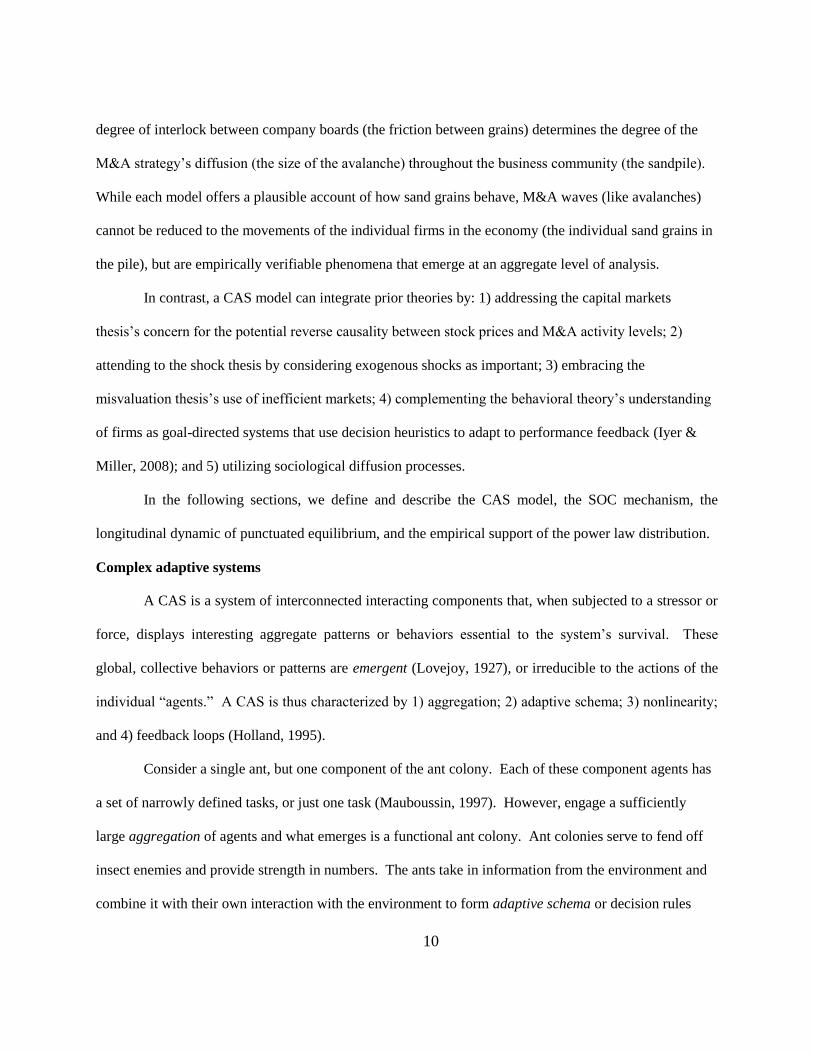
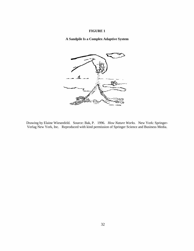
an integrative model. The central intuition is best illustrated by a pile of sand (Bak et al., 1987), as shown

in Figure 1.

---------------------------------------

Insert Figure 1 about here

---------------------------------------

Adding sand grains sequentially onto a flat surface generates a pile with an increasingly steep

slope until, at a critical point, an avalanche occurs, collapsing the pile. A larger pile of sand or a faster

addition of sand grains can potentially generate more frequent and larger avalanches. Poking the pile

with one’s finger generates an avalanche in the poked region of the pile; likewise, poking the pile with

9

multiple fingers results in multiple avalanches which may combine to affect more of the pile. The unique

physical properties of the grains—their mass and volume, for example—suggest that gravity acts upon

them during avalanches to generate smooth slopes. Because the friction between adjacent grains

influences the likelihood of an avalanche, a wet pile of sand will be less likely to collapse while a dry pile

of sand is more likely to collapse (Bak et al., 1988). After enough grains are dropped onto the pile, an

avalanche occurs, collapsing the pile until a sufficient amount of additional grains has again been

deposited, suggesting a pattern over time of short periods of substantial movement alternating with longer

periods of relative calm. The avalanches themselves cannot be reduced to the individual movements of

the sand grains, but rather are empirically verifiable phenomena that emerge at an aggregate level of

analysis.

Analogizing from the sandpile to M&A activity shows the theoretical value of a CAS model.

M&As (the dropped sand grains) occur all the time, but most do not generate a M&A wave (an

avalanche) unless some apparently critical point is reached. The capital market thesis argues that high

stock prices (the larger sand pile representing the macroeconomy) are correlated with high M&A activity

(the faster addition of sand grains representing more M&A deals), and vice versa. The extant models of

M&A waves described earlier represent attempts to theorize largely at the level of the sand grain. The

firm misvaluation thesis argues that each new misvalued M&A (each new dropped grain of sand)

motivates other, less misvalued M&As (the tension in the sand pile) until their true value is revealed, at

which point the M&A market crashes (an avalanche). Behavioral scholars suggest that organizations (the

grains of sand) are uniquely goal-directed systems (i.e. the unique properties of the sand) that respond

deterministically to performance feedback (i.e., the law of gravity). The shock thesis argues that a

disturbance to an industry (i.e., poking a finger in a region of the pile) can set off an industry M&A wave

(a local avalanche), while multiple disturbances across industries (poking multiple fingers in the pile) can

generate an aggregate M&A wave (a combination of regional avalanches). Sociologists believe that the

10

degree of interlock between company boards (the friction between grains) determines the degree of the

M&A strategy’s diffusion (the size of the avalanche) throughout the business community (the sandpile).

While each model offers a plausible account of how sand grains behave, M&A waves (like avalanches)

cannot be reduced to the movements of the individual firms in the economy (the individual sand grains in

the pile), but are empirically verifiable phenomena that emerge at an aggregate level of analysis.

In contrast, a CAS model can integrate prior theories by: 1) addressing the capital markets

thesis’s concern for the potential reverse causality between stock prices and M&A activity levels; 2)

attending to the shock thesis by considering exogenous shocks as important; 3) embracing the

misvaluation thesis’s use of inefficient markets; 4) complementing the behavioral theory’s understanding

of firms as goal-directed systems that use decision heuristics to adapt to performance feedback (Iyer &

Miller, 2008); and 5) utilizing sociological diffusion processes.

In the following sections, we define and describe the CAS model, the SOC mechanism, the

longitudinal dynamic of punctuated equilibrium, and the empirical support of the power law distribution.

Complex adaptive systems

A CAS is a system of interconnected interacting components that, when subjected to a stressor or

force, displays interesting aggregate patterns or behaviors essential to the system’s survival. These

global, collective behaviors or patterns are emergent (Lovejoy, 1927), or irreducible to the actions of the

individual ―agents.‖ A CAS is thus characterized by 1) aggregation; 2) adaptive schema; 3) nonlinearity;

and 4) feedback loops (Holland, 1995).

Consider a single ant, but one component of the ant colony. Each of these component agents has

a set of narrowly defined tasks, or just one task (Mauboussin, 1997). However, engage a sufficiently

large aggregation of agents and what emerges is a functional ant colony. Ant colonies serve to fend off

insect enemies and provide strength in numbers. The ants take in information from the environment and

combine it with their own interaction with the environment to form adaptive schema or decision rules

11

(Gell-Mann, 1995) which compete according to their utility, creating adaptive behavior. CAS are also

nonlinear: the aggregate behavior is more complicated than would be predicted by summing the parts

(Mauboussin, 1997). For example, a basic predator/prey model with ―feast and famine‖ patterns is

generated from the product of variables, not the sum, such that cause and effect relationships are no

longer simply linear (ibid). Positive feedback loops occur when the output of one iteration becomes the

input of another iteration, thus amplifying the effect, much like how an electric guitar amplifies the noise

generated by the speaker it is plugged into, generating audio feedback. Positive feedback loops generate

potentially explosive, self-reinforcing and destabilizing behaviors. Conversely, negative feedback loops

dampen a system’s response to a stimulus.

Now let us analogize to firms. In the economic sense, individual firms have two basic tasks: (1)

consume inputs and (2) produce outputs. But engage a sufficiently large aggregation of firms, with one

firm’s output being another firm’s input, and the outcome is a thriving economy replete with competitive,

cooperative, and predatory firm behaviors (such as M&A). Firms engage in these adaptive behaviors

through the decision-rules obtained from the performance feedback managers receive from the

surrounding economic environment. An M&A of one firm changes the competitive stance of nearby

firms, and their subsequent interdependent actions and reactions may result in feedback loops among the

firms, setting off surges of M&A. This predator-prey dynamic between acquirers and targets generates

the non-linear ―feast and famine‖ pattern of emergent M&A waves alternating with long stretches of little

M&A activity.

Self-organized criticality

CAS naturally evolve to the self-organized critical (SOC) state, when they transition from mere

collections of individual agents into vibrant emergent phenomena (Bak, 1996) poised far out of

equilibrium (Bak & Sneppen, 1993). As shown in Figure 1, adding more grains to a sand pile leads to

more avalanches every time the critically steep slope is reached, so that the pile ―self-organizes‖ to this

12

state. Avalanches are the mechanisms for the SOC system to dissipate built-up tension and energy in a

non-linear return to unstable equilibrium, much like earthquakes that violently dissipate the accumulated

tension of continental plates when the earth’s crust cracks. Analogously, economies can also be SOC.

Suppose M&A activity (like dropping sand grains) occurs at a nominal, ―linear‖ rate in an economy.

None of the individual M&As may immediately incite a wave. But each additional deal, like each falling

grain of sand, adds to the instability under the seeming stasis. Once the economy achieves the SOC state,

an additional M&A can unleash an outbreak of deals. These M&A waves are SOC phenomena

expressing a non-linear return to dynamic equilibrium (Morel & Ramanujam, 1999).

Punctuated equilibrium

CAS are ―alive,‖ and their activity over time is one of relative equilibrium interrupted by

catastrophic instabilities, similar to mass extinctions in the fossil record. Kauffman (1993) has argued

that life itself, in its nonlinear evolution over time and its admixture of inert order and random chaos, is

complex. Do M&A patterns over time express an evolutionary dynamic similar to that of biological

evolution?

If so, perhaps their overall development and change embody punctuated equilibrium (Eldredge &

Gould, 1972). Punctuated equilibrium theory positions itself in distinction from the Darwinist argument

for gradual smooth evolutionary change. In a biological ecosystem, long periods of incremental

evolutionary change are ―punctuated‖ by mass extinctions which precede periods in which the ecology

undergoes a fast rebuild, hence the appearance of so many new species seemingly instantaneously.

For example, consider an ecosystem comprising organisms, species and the surrounding habitat.

Ongoing natural selection aggregates random changes over many successive generations of species as the

less fit are naturally ―discarded,‖ so the interaction of interdependent organisms is relatively stable most

of the time. But at some point in time, a significant advantageous variation cumulates to a species’

organisms, leading quickly to frustrated and intensified predation of predator and prey species,

13

respectively. These species, in turn, become ravaged, and their sad fate in turn harms other related

predators but benefits other related prey. Thus, one adaptation in a single organism or species can trigger

mass extinctions throughout the entire ecosystem.2

Analogously, consider organisms as firms, species as industries, and the economy as their habitat.

The adaptation processes of evolution proceed in natural selection as the aggregated effect of random

M&A activity as less ―fit,‖ i.e. economically viable, firms naturally become ―extinct,‖ i.e. acquired. For

long periods, this competitive dynamic among firms is relatively stable. But over time, some firms accrue

slack resources in interacting with competitors, and these firms build on their adaptive success by

engaging in M&As (Iyer & Miller, 2008) which represent the subsuming of a firm by a ―fitter‖ one in an

ecological niche (Bak & Sneppen, 1993). Soon thereafter, intraindustry competitors become horizontal

M&A targets as the adapted firms sow the seeds for future generations of the industry/species. Along the

value chain, ―prey‖ firms providing inputs to the adapted firms or ―predator‖ firms consuming adapted

firms’ outputs become preemptive targets of vertical integration. The adapted firms also diversify vis-à-

vis M&A as they interact in selection processes and establish symbiotic relationships with other species’

organisms, i.e., with related and unrelated industries’ firms. Eventually, whole industries-species

compete with other industry-species, resulting in mass firm extinctions: an aggregate M&A wave. Thus,

a single M&A deal can trigger off an aggregate M&A wave throughout the entire economy.

The power law signature

In punctuated equilibrium, a CAS builds up evolutionary pressures over long periods of seeming

stasis until the SOC state is reached, destabilizing the system and generating sudden bursts of systemic,

revolutionary change. This pattern violates Gaussian assumptions that extreme events happen but rarely,

that the future can be predicted from the past, and that linear proportional cause-effect relationships hold.

2 Bak & Sneppen (1993) modeled punctuated equilibrium of species in an ecosystem by simulating their adaptive

mutations and interdependencies, an exercise that produced intermittent bursts of evolutionary activity alternating with long periods of calm.

14

In contrast, Paretian statistics seem to fit a punctuated equilibrium account of waves better. In a Paretian

world, the past is not a good predictor of the future, small causes can have big effects (or large influences

can lead to insignificant outcomes), and large earthquakes, stock market crashes, torrential floods and

mass epidemics occur often.3 Likewise, M&A waves are hard to predict, their purported causes are

disproportionately small to the wave effect, and they are non-trivial and extreme events.

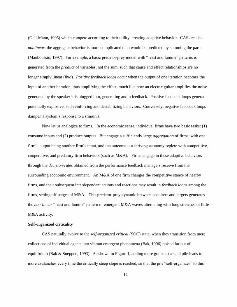
But how can we test whether a phenomenon hews to the CAS model? By observing a Paretian

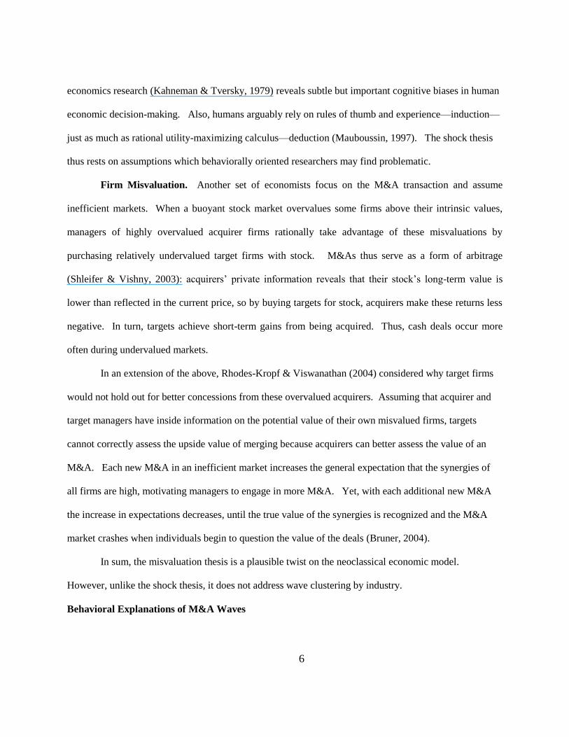
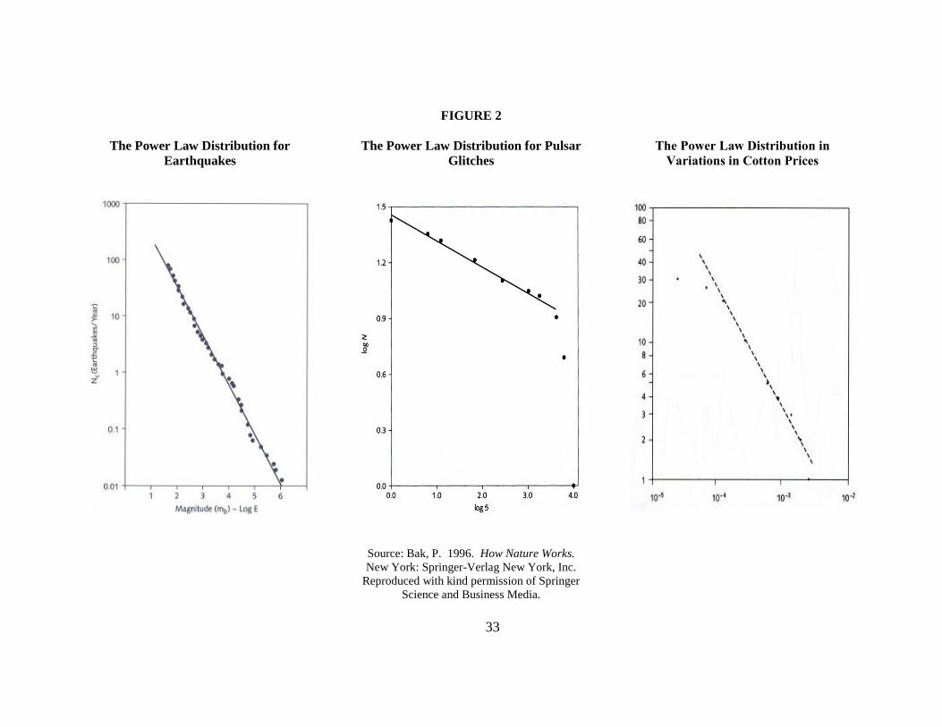
power law distribution for the wave system. Bak, Tang and Wiesenfeld (1987, 1988) originally described

the spatial and temporal ―fingerprint‖ of the SOC state as ―1/f noise,‖ or the power law distribution, (also

known as Zipf’s law or the Pareto distribution). Some real-world power laws are shown in Figure 2. For

example, in geophysics, for every 1000 earthquakes of magnitude 4 on the Richter scale, there are 100

magnitude-5 earthquakes, 10 of magnitude 6, and so on. A similar mathematical relationship holds for

pulsar glitches. Pulsars are stars made up of neutrons spinning at high velocity. Glitches of all sizes

happen when the pulsar’s rotation changes suddenly. The relationship of a glitch’s size to its frequency of

occurrence follows a power law. Benoit Mandelbrot in 1966 recorded the number of months in which

cotton prices changed from the prior month by 10% – 20%, 5% - 10%, and so on. The relationship of the

number of months to percent variation follows a power law.

-----------------------------------------

Insert Figure 2 about here

-----------------------------------------

The power law, Zipf’s law and the Pareto distribution are mathematically equivalent. George

Zipf, a Harvard linguistics professor, initially examined the ―size‖ or frequency of words in an English

text. Zipf's Law states that the size of the rth largest occurrence of the event is inversely proportional to

its rank:

y ~r-b

,

3 In other words, traditional statistical analysis is Gaussian; a power law distribution reflects a Paretian dynamic.

15

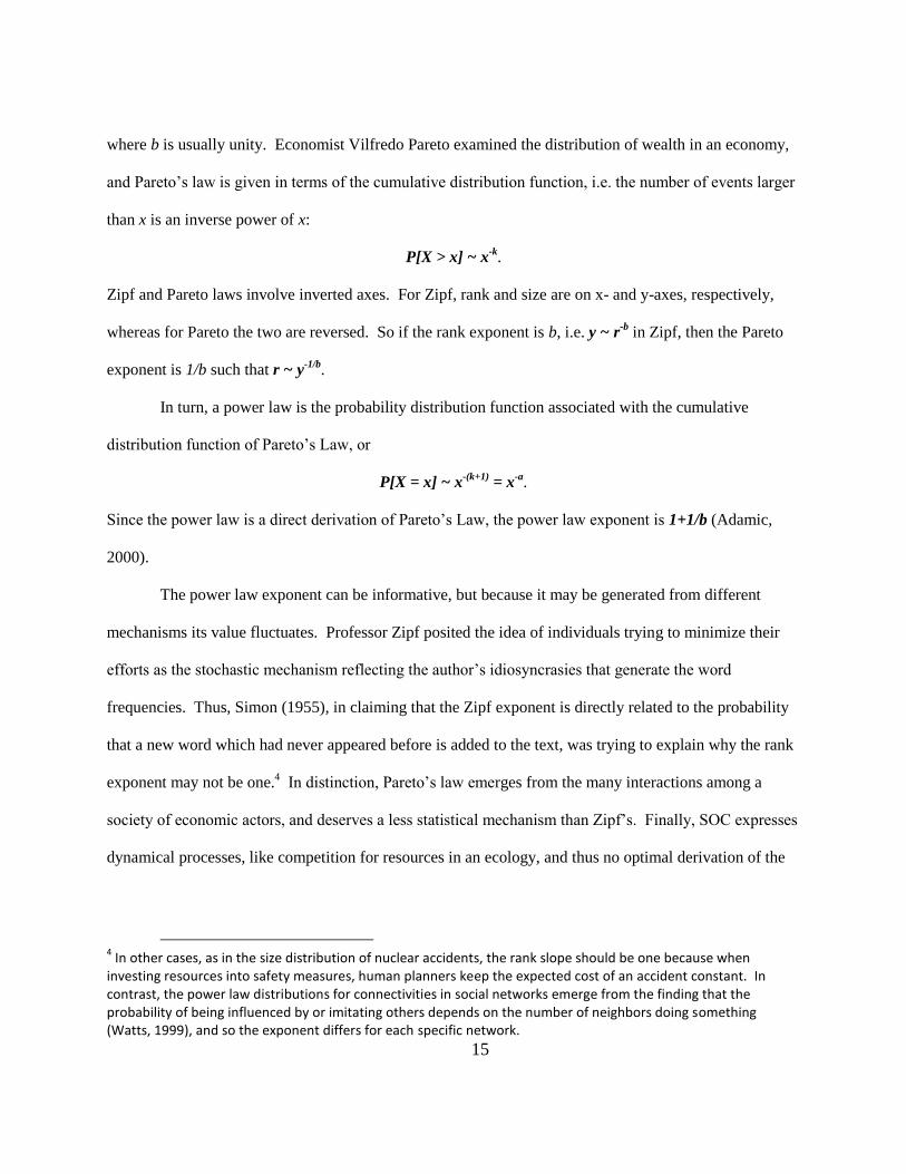
where b is usually unity. Economist Vilfredo Pareto examined the distribution of wealth in an economy,

and Pareto’s law is given in terms of the cumulative distribution function, i.e. the number of events larger

than x is an inverse power of x:

P[X > x] ~ x-k

.

Zipf and Pareto laws involve inverted axes. For Zipf, rank and size are on x- and y-axes, respectively,

whereas for Pareto the two are reversed. So if the rank exponent is b, i.e. y ~ r-b

in Zipf, then the Pareto

exponent is 1/b such that r ~ y-1/b

.

In turn, a power law is the probability distribution function associated with the cumulative

distribution function of Pareto’s Law, or

P[X = x] ~ x-(k+1)

= x-a

.

Since the power law is a direct derivation of Pareto’s Law, the power law exponent is 1+1/b (Adamic,

2000).

The power law exponent can be informative, but because it may be generated from different

mechanisms its value fluctuates. Professor Zipf posited the idea of individuals trying to minimize their

efforts as the stochastic mechanism reflecting the author’s idiosyncrasies that generate the word

frequencies. Thus, Simon (1955), in claiming that the Zipf exponent is directly related to the probability

that a new word which had never appeared before is added to the text, was trying to explain why the rank

exponent may not be one.4 In distinction, Pareto’s law emerges from the many interactions among a

society of economic actors, and deserves a less statistical mechanism than Zipf’s. Finally, SOC expresses

dynamical processes, like competition for resources in an ecology, and thus no optimal derivation of the

4 In other cases, as in the size distribution of nuclear accidents, the rank slope should be one because when

investing resources into safety measures, human planners keep the expected cost of an accident constant. In contrast, the power law distributions for connectivities in social networks emerge from the finding that the probability of being influenced by or imitating others depends on the number of neighbors doing something (Watts, 1999), and so the exponent differs for each specific network.

16

power law exists, only evidence vis-à-vis ―cellular automata‖ like Bak et al.’s (1987) sand piles.

Therefore, the interpretation of the value of the exponent is ultimately context dependent.

Power law-distributed M&A waves would imply that they are SOC and that a CAS model of

waves is a good fit to the phenomenon. This is because power laws imply systemic instability vis-à-vis

SOC, a known mechanism for generating complexity (Bak, 1996). SOC waves would thus be the

mechanisms for dissipating the accumulated tension of long-range forces in the M&A system, returning it

to dynamic equilibrium in a non-linear fashion. Further, M&A waves would share the same underlying

mechanism generating complex behavior as in avalanches for sandpiles, earthquakes for tectonic plates,

glitches for pulsars and price variations for commodities markets.

METHODOLOGY

For our empirical analysis, we first obtained a complete time-series of M&A activity. We then

analyzed the data with a wave-identification procedure to create a Zipf plot.

Obtaining U.S. M&A data

We used Town’s (1992) z-score data covering 1895:1-1989:1, at the Research Papers in

Economics (RePEc) website: http://ideas.repec.org/p/boc/bocins/merger.html. We added z-scores from

1989:2–2008:2. We sought consistency with the inclusion criteria of the four series comprising Town’s

(1992): Nelson (1959) 1895:1–1919:4; Thorp (listed in Nelson, 1959) 1920:1–1954:4; the Federal Trade

Commission’s (FTC) Large Merger Series 1955:1–1979:4; Mergers and Acquisitions Magazine 1980:1–

1989:1. Each source, except for the non-appraised Thorp series, differed from the others on one or more

of the following categories: (1) public vs. private transactions; (2) whole or partial deals; (3) U.S. or non-

U.S. buyers; (4) announcement date vs. completed/effective date; (5) industry inclusion.

Public transactions only. All series except for M&A magazine included only publicly listed

firms, so we excluded private transactions.

17

100% whole M&A deals. Nelson utilized whole firm disappearances; FTC did not distinguish

between full and majority deals; and M&A magazine included deals of 5% ownership or more changing

hands. We chose 100% whole ownership deals, since M&As should represent a significant shift in the

market for corporate control.

U.S. and non-U.S. buyers of U. S. targets. Nelson mentioned no cross-border deals, but FTC

and M&A magazine included non-U.S. buyers. Furthermore, U.S. M&A by non-U.S. buyers represented

an increasingly significant portion of the M&A market from 1989-2008.

Announcement date (of completed deals). Nelson, FTC and M&A magazine were based on

announcements in the financial press, and SDC provided announcement dates. We included completed

announced deals since Nelson considered long-standing firm disappearances, FTC took into account

consummated deals, and M&A Magazine removed cancelled deals.

All industries. Manufacturing and mining for Nelson and FTC comprised the majority of the

U.S. economy then (although this is debatable toward the end of FTC). M&A magazine included all

industries in its universe of firms. Thus, we included all industries for 1989-2008 to capture the overall

economy.

We then normalized and standardized the raw data. SDC records corporate transactions of $1

million and over from 1979–1992, and all deals from 1993-present. Coverage in SDC from 1979-1982 is

spotty, and not all items were available. Therefore, for 1983:1-1992:4 we divided the number of M&As

by the yearly number of active U.S. corporations with assets above US $1 million, and for 1993:1-2008:1,

by the yearly number of all active U.S. corporations. We obtained data on corporations 1990–2005 from

the Internal Revenue Service’s Statistics of Income online at

http://www.irs.gov/taxstats/article/0,,id=175843,00. html. We standardized the two series (1983:1-1992:4

and 1993:1-2008:2) per the equation

y

y

y

yn

where yt is the series and μy and σy are the sample

18

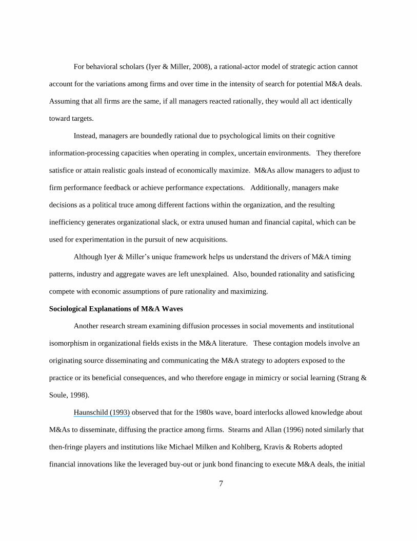
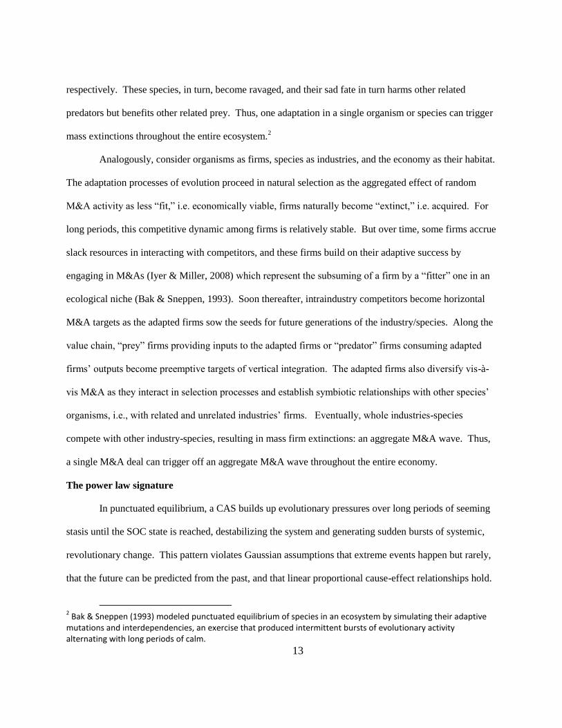
mean and standard deviation of yt, respectively. Figure 3 below shows the resulting time-series of

aggregate U.S. M&A activity from 1895 through 2008.

--------------------------------

Insert Figure 3 about here

--------------------------------

Defining a Wave

We sought to improve on existing wave identification methods. Carow et al. (2004) identified

heightened periods of annual M&A activity from inception to peak and back down in six-year windows.

Harford (2005) detected the highest concentration of industry M&A activity in 24-month windows, and

compared the frequency to the 95th percentile of simulations. McNamara et al. (2008) used both

procedures and also required that M&As increase over 100% from the base year and decrease by over

50% from peak year, in six-year windows. In contrast, we avoided arbitrary time windows and

probabilistic simulations in favor of a more rigorous approach.

We employed strucchange in R (Bai & Perron, 2003; Zeileis, Kleiber, Krämer, & Hornik,

2003; Zeileis, Leisch, Hornik, & Kleiber, 2002), which tests for structural change in linear regression

models. For Figure 3, it recorded significant shifts in the mean of the series but disregarded random

noise. We defined a M&A wave as a significant upward structural change from a baseline z = 0 M&A

activity to a peak, with a subsequent significant decrease below z =0. The minimum wave length was set

as three quarters (beginning, middle and end). Strucchange produced 27 ―breakpoint‖ quarters where

mean shifts occurred, creating 28 segments. We identified changes in the series mean from negative to

positive and back to negative. A wave began with the quarter after the breakpoint separating a negative

from a positive segment. The wave ended with the breakpoint quarter (inclusive) preceding the next

negative-mean segment. At one point a negative trough preceded a positive peak, descended to a positive

trough, and then increased to a positive peak before descending to a negative-mean trough. Therefore,

the first wave ended at the breakpoint quarter (inclusive) separating the first positive-mean peak and the

19

positive-mean trough. The second wave began with the quarter after the breakpoint separating the

positive-mean trough from the second peak. Consequently there was no overlap between the two waves,

and they were not considered adjacent to each other.

For wave size, we considered amplitude (highest z-score), duration (length in quarters), a

combination of amplitude and duration, and intensity (average z-score). For Zipf’s Law, we ranked the

waves by intensity from largest to smallest, placing ―1‖ first, and plotted rank to size.

RESULTS

Table 1 presents the descriptive statistics.

---------------------------------

Insert Table 1 about here

---------------------------------

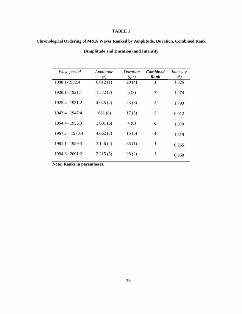
Table 1 lists the waves in chronological order with the rankings. Strucchange dates the historical

M&A waves more accurately than anecdotal evidence: 1898:1–1902:4, 1925:4–1931:2, 1967:2–1970:4,

1981:1–1989:3 and 1994:3–2001:2. In terms of amplitude, the 1890s wave was the largest in recorded

history, with the 1920s wave placing second, the 1960s wave in third, and the 1980s and 1990s waves

finishing fourth and fifth, respectively. The duration rankings show the 1980s wave as the longest, the

1990s wave second longest, the 1920s wave in third place and the 1900s wave in fourth place. The 1960s

wave comes in sixth, with a post-WWII wave in fifth place. Missing from the accounts of Bruner (2004),

Ravenscraft (1987) and Scherer & Ross (1990)—notable M&A scholars who list the same five largest

M&A waves—are M&A spikes in 1920-1921 and 1954-1955 (that admittedly rank lowest).

The amplitude and duration rankings are at odds with each other and previous accounts.

However, if we weigh the two metrics equally, a more historically congruent picture emerges, as shown

in the combined ranking of Table 1: tied for first, (1) 1900s and 1980s, (3) 1990s, (4) 1960s and (5)

20

1920s.5 The last three smallest waves—1920:1–1921:1, 1943:4–1947:4 and 1954:4–1955:3—are

mentioned in Nelson (1959), who lists them as 1920, 1946-47 and 1954-56, respectively. Town (1992)

corroborates, with waves identified at 1919:2–1921:4, 1945:4–1946:1 and 1954:3–1955:3. Town further

adds 1960:1–1960:2 and 1962:1–1962:2. These last two were not listed by Bruner, Ravenscraft or Sherer

and Ross, and were not detected by strucchange, presumably because a wave had to be at least three

quarters long.

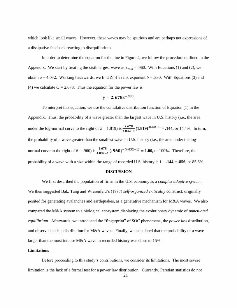
To combine the amplitude and duration metrics into a general intensity ranking we averaged the

z-scores of the quarters comprising each wave. The results, shown in the right column of Table 1, reveal

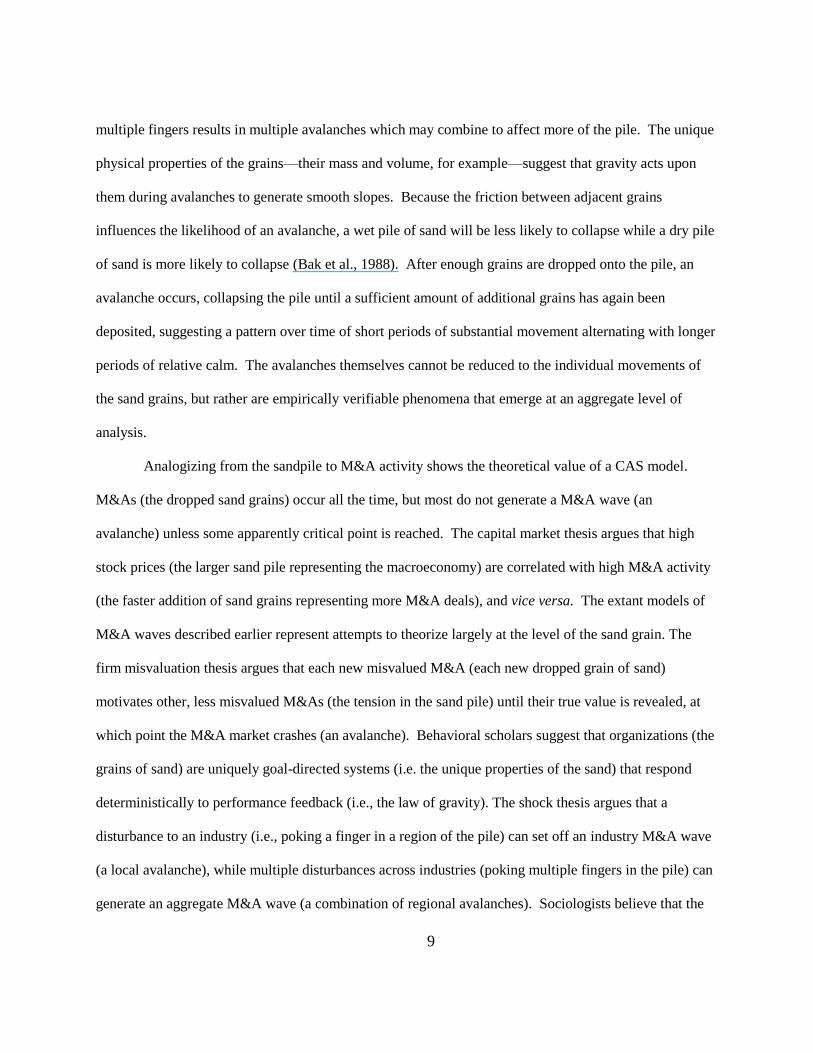
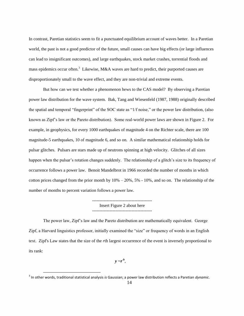
that the largest wave is 𝑧 = 1.819 and the smallest is 𝑧 =.012. Figure 4 shows Zipf’s law for M&A waves

by intensity on log-log paper, revealing the power law signature, a line of negative slope connecting all

but two small waves.

-------------------------------

Insert Figure 4 about here

-------------------------------

These last two waves may signify a threshold for a dissipative return to dynamic equilibrium to

occur via M&A (similar to how the three smallest pulsar glitches in Figure 3 fall off the power law). In

other words, M&A activity is continuous, meaning that M&As are simply routine in the life of some

firms, as when small entrepreneurial biotech start-ups are acquired by large established pharmaceutical

firms to exploit a new drug discovery, or when large computer software firms take over search engine

sites to outsource that activity. These M&A do not generate dissipative effects. Of course, because

M&A activity’s stochastic nature generates uneven distributions in time there may be some fluctuations

5 To combine the two rankings, we first compared both for each wave, and chose the higher of the two to represent

the wave rank. In the case of a tie between two waves, we gave precedence to the wave for which the second-

category rank was higher. For example, the 1920s wave ranked second in amplitude and third in duration, while the

1990s wave ranked fifth in amplitude and second in duration. By ranking with the higher number, these two waves

were tied for second. But because the 1920’s wave was ranked third and the 1990’s wave was ranked fifth in the

secondary category, the former was ranked second, and the 1990’s wave placed third.

21

which look like small waves. However, these waves may be spurious and are perhaps not expressions of

a dissipative feedback reacting to disequilibrium.

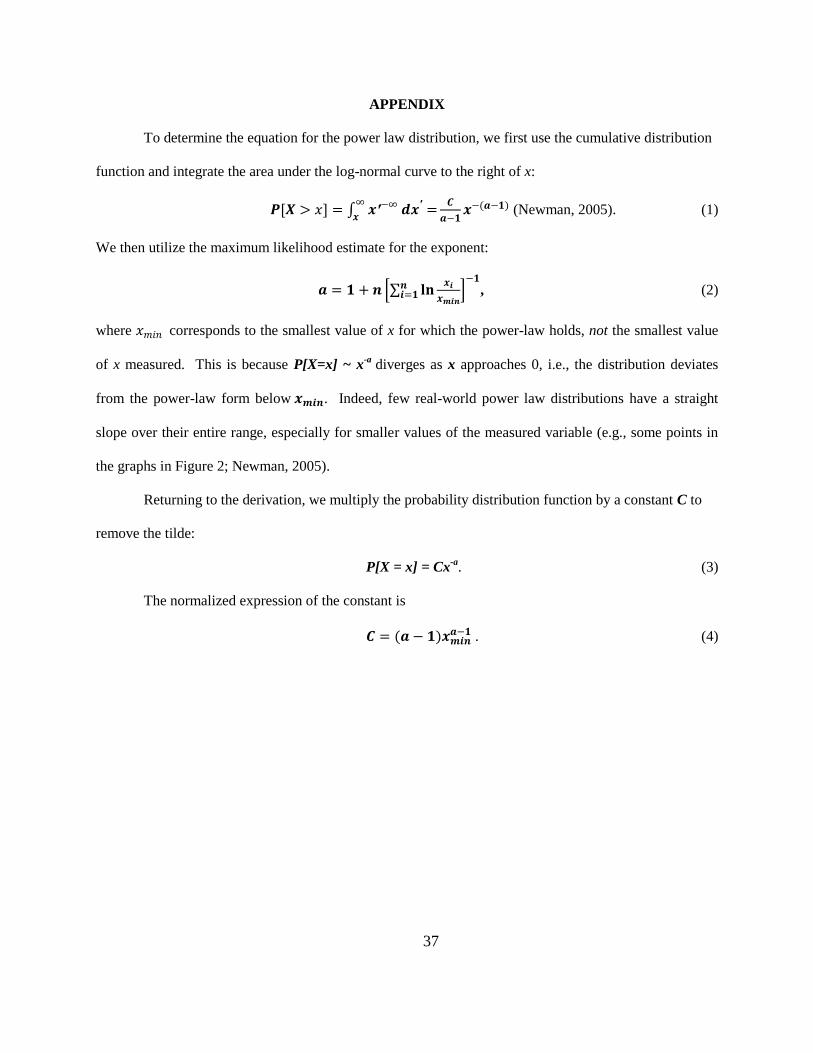
In order to determine the equation for the line in Figure 4, we follow the procedure outlined in the

Appendix. We start by treating the sixth largest wave as 𝑥𝑚𝑖𝑛 = .960. With Equations (1) and (2), we

obtain a = 4.032. Working backwards, we find Zipf’s rank exponent b = .330. With Equations (3) and

(4) we calculate C = 2.678. Thus the equation for the power law is

𝒚 = 𝟐. 𝟔𝟕𝟖𝒙−.𝟑𝟑𝟎.

To interpret this equation, we use the cumulative distribution function of Equation (1) in the

Appendix. Thus, the probability of a wave greater than the largest wave in U.S. history (i.e., the area

under the log-normal curve to the right of 𝑧 = 1.819) is 𝟐.𝟔𝟕𝟖

𝟒.𝟎𝟑𝟐−𝟏

(1.819)

-(4.032 - 1) = .144, or 14.4%. In turn,

the probability of a wave greater than the smallest wave in U.S. history (i.e., the area under the log-

normal curve to the right of 𝑧 = .960) is 𝟐.𝟔𝟕𝟖

𝟒.𝟎𝟑𝟐−𝟏(. 𝟗𝟔𝟎)−(𝟒.𝟎𝟑𝟐−𝟏) = 1.00, or 100%. Therefore, the

probability of a wave with a size within the range of recorded U.S. history is 1 – .144 = .856, or 85.6%.

DISCUSSION

We first described the population of firms in the U.S. economy as a complex adaptive system.

We then suggested Bak, Tang and Wiesenfeld’s (1987) self-organized criticality construct, originally

posited for generating avalanches and earthquakes, as a generative mechanism for M&A waves. We also

compared the M&A system to a biological ecosystem displaying the evolutionary dynamic of punctuated

equilibrium. Afterwards, we introduced the ―fingerprint‖ of SOC phenomena, the power law distribution,

and observed such a distribution for M&A waves. Finally, we calculated that the probability of a wave

larger than the most intense M&A wave in recorded history was close to 15%.

Limitations

Before proceeding to this study’s contributions, we consider its limitations. The most severe

limitation is the lack of a formal test for a power law distribution. Currently, Paretian statistics do not

22

admit of formal tests of power laws comparable to tests of linearity in Gaussian statistics. Furthermore,

many rank/frequency plots often follow power laws primarily in the tail of the distribution. The only

alternative would have been to collect a sample size of waves large enough to analyze and test their

distribution. However, over a 113-year period strucchange only produced eight waves, of which two

were appropriately discarded. And given that the six remaining M&A waves clearly matched other

scholarly and anecdotal accounts, the chosen methodology properly generated the correct data structure;

yet, we cannot offer an absolute, definitive conclusion. Notwithstanding the exploratory nature of this

investigation, we feel that the CAS model has much to offer. Some of those insights we share below.

Embracing Existing Theory

Our CAS model serves to integrate previous theories. First, regarding the capital markets thesis,

it may be that the stock market itself is a CAS that displays emergent properties (Sornette, 2003). For

example, financial markets are comprised of millions of interdependent economic actors whose aggregate

patterns include emergent stock price bubbles and crashes. Thus, the potential reverse causality between

M&A activity and the stock market during bubbles may be a manifestation of a positive feedback loop, in

which a rising trend in the former amplifies and effects a rising trend in the latter, and vice versa.

Similarly, a negative feedback loop during stock market and M&A market busts involves a decreasing

trend in the stock markets heavily dampening M&A activity levels, and vice versa. Thus, M&A activity

oscillates from frozen inactive states to ―hot‖ disordered states (Bak & Sneppen, 1993) in response to the

stock market in a non-linear, predator/prey type dynamic.

Second, regarding the industry shocks thesis, if external shocks generated waves, we would

expect a peak in the distribution at large events, which runs counter to the evidence. Shocks happen, but

they may not be the primary cause, just as the cracking of the earth’s crust is the more visible external

trigger for earthquakes, while the underlying friction between tectonic plates is the less visible but more

23

basic reason.6 Analogously, an industry shock may hasten an M&A wave as the more visible but

ultimately less important precursor. Instead, evolutionary pressures in the firm ecology that have built up

over time are the less visible but more fundamental triggers.

Third, regarding the competing market (in)efficiency and (ir)rational actor assumptions of the

industry shock and firm misvaluation theses, complexity theory clearly suggests that during M&A waves,

firm behavior is irrationally herd-like in a ―cooperative,‖ inefficient M&A market, analogous to how the

grains of sand in a sandpile naturally slide and fall together to generate a powerful avalanche. However,

during non-wave periods, traditional neoclassical economic assumptions concerning efficiency and

competition hold, as suggested in the stillness of a sand pile as individual grains are added one-by-one

(which can be explained by classical physics). Furthermore, at the SOC state, when the ecology of firms

(like the pile of sand) is just barely stable with respect to further perturbations, firm behavior is based on

cooperation and competition to respond adaptively to the environment in the name of survival.

Fourth, a CAS model can generate the industry waves lacking in the firm misvaluation thesis.

The biological ecosystem metaphor describes how mass extinctions (aggregate M&A waves) begin with

certain organisms (firms) achieving evolutionary fitness sooner than competitors to become ―progenitors‖

for the rest of the species (industry). Soon thereafter, predator and prey species (industries along the

value chain) become endangered (become vertical integration targets). Meanwhile, the fitter organisms

establish new relationships with other, previously uninvolved prey species (other firms in related and

unrelated industries become diversification targets). Thus, industry waves can occur with aggregate

waves.

Fifth, we think a CAS model agrees with the behavioral theory’s conception of firms as open,

goal-directed systems that use simple decision heuristics to adapt responsively to performance feedback.

6 Similarly, some evolutionary biologists have suggested that an exogenous meteorite impact caused the dinosaurs’

extinction, but arguably the dinosaurs were by then already becoming extinct (Bak, 1996). Rather than being the prime mover, a meteorite impact hastened extinction.

24

Managers utilize M&A as a convenient adaptation response to organizational slack and falling

performance aspiration levels. The goal of a CAS is survival, and the decision heuristics are reminiscent

of the adaptive schema that complex systems use to learn by directing and modifying behavior to shifting

environmental contexts. Such heuristics are not consciously derived per se (though there is a logic to

them), but they are not purely based on instinct either (though there is an effortlessness to them). Rather,

this juncture characterizes the SOC state, where the CAS is most visibly alive.

Sixth, regarding sociological theories, they, too, draw from complexity theory. Watts (1999)

suggested that the probability of being influenced by or imitating others depends on the number of

neighbors doing something. A power law mathematically satisfied this description, i.e., most nodes in a

social network are related to a few neighbors, while a much smaller number of ―hub‖ actors are

disproportionately connected to a very large number of neighbors. Such a structure allows for small local

changes to lead to large-scale global cataclysms; alternatively, the same network may be robust to a

significant mutation. In other words, a single localized M&A may create cascade or ―percolation‖ effects

throughout the entire business community, while conversely the global effect of a large number of

simultaneous M&A transactions may be quite minimal. Such scale-free networks may serve an

evolutionary raison d’être (Barabasi & Albert, 1999), as if M&A waves are virus-like ―infections‖ that

spread throughout a weakened host (while non-wave periods signal an organism’s immunity to disease).

These may indicate a business community’s weakness (as well as resistance) to a corporate strategy

―syndrome.‖

A CAS model of SOC M&A waves may also explain why fringe actors and innovations abruptly

arise in a business community. The endogenous process begins with the community in a relatively

unagitated state, with the occurrence of few M&A deals, but underneath the seeming stability are

macroeconomic forces that push the community towards disequilibrium, leading to large waves of

dealmaking. The existence of challenger actors and financial innovations (Stearns & Allan, 1996)

25

indicate a SOC business community, similar to the critical slope of a SOC sandpile right before an

avalanche or the stressed position of SOC tectonic plates immediately before a earthquake. The

challenger actors and financial innovations may be the early-warning indicators of M&A waves.

Managerial Implications and Future Research

Apart from being academic curiosities, M&A waves also present opportunities for value-creation

(or destruction). Moeller, Schlingemann and Stulz (2005) observed that acquiring-firm shareholders

gained $24 billion from 1991 through 1997—the start of the 1990s M&A wave—before losing $240

billion at the end of the wave, from 1998 through 2001. Given this and the large probability of another

M&A wave at some point in the future, it is important to know when the next one will happen. Yet at

first glance the managerial relevance of the complexity perspective may seem limited. The indeterminacy

of complex systems makes prediction difficult, and their inherent variability makes feasible only a

narrative account of distinguishable events post mortem (Bak, 1996).

But as Goldstone (1991) noted, geologists may not be able to predict the precise number and

location of fossils in a particular sort of rock, but can predict the types of fossils and their rough

proportions if they know that the rock was formed at a time when certain species lived. Likewise, waves

are unique in terms of timing, amplitude, duration and strategic motivation, thus precluding exact

prediction, but they do share certain recognizable, generic patterns that managers can identify as the

patterns emerge before an oncoming M&A wave. In other words, scholars can identify 1) similar (but not

identical) initial conditions with which 2) regular laws would produce 3) similar (but not identical or

exactly predictable) results—a robust process (ibid.). For example, (1) runaway consumer demand may

intensify investment in property, plant and equipment vis-à-vis M&A; (2) low interest rates may induce

heavy borrowing to leverage more speculative M&A transactions; and (3) pro-business economic policies

may allow more M&A deals to avoid anti-trust scrutiny. A combination of such processes may generate

M&A waves, and timely adaptation to them may be built around identifying and preparing for such

26

processes. Thus, from a managerial viewpoint, it may be more important to strive for situational

awareness combined with fast response rather than for (an unattainable) predictive capacity.

Other compelling managerial implications come from the analogies to other SOC phenomena.

Bak, Tang and Wiesenfeld (1988) noted that the angle of repose is higher for a pile of wet sand so that as

the water evaporates, small and large avalanches occur at random places on the pile. If ―sticky,‖ wet sand

grains are more resistant to avalanches, perhaps firms with many inter-organizational linkages—―sticky

linkages‖—are more capable of withstanding takeovers during M&A waves. Sticky linkages are similar

to equity strategic alliances, but are more accurately a set of cross-shareholdings between a focal firm and

its broad constellation of stakeholders, like Japanese keiretsu firms with vertical relationships connecting

all factors of production of a certain product, and horizontal relationships with owner banks and trading

companies. In contrast, U.S. firms may be embedded in an atomistic social, economic, legal, political and

institutional ―fabric‖ loosely comprised of antagonistic constituencies. This implies that fostering sticky

linkages among U.S. entities may ameliorate the likelihood of disruptive acquisition during M&A waves

by weaving a strong, localized ―safety net‖ comprised of law firms, investment banks, shareholders, the

government, suppliers, and customers. By aligning their interests, these stakeholders may generate in-

group keiretsu-like biases that keep opportunistic ―outsider‖ acquirers at bay and foster ―thick‖ internal

cross-ownership structures. On the other hand, existing financial market and anti-trust regulations have

the express purpose of acting as a counterweight to such embedding tendencies – leading both to robust

markets for corporate control and to M&A waves.

CONCLUSION

Prior research on M&A waves, drawn from often conflicting scholarly disciplines, has produced

reductionist models that throw little light on the emergent properties of such waves. Our CAS model

provides a more integrated account, and generates a useful metaphor to facilitate managerial

27

understanding and preparation for M&A waves . While but an initial step, we hope our work enriches

future studies on this fascinating and important phenomenon.

28

REFERENCES

Adamic, L. A. 2000. Zipf, Power-law, Pareto - a ranking tutorial: Hewlett-Packard.

Bai, J., & Perron, P. 2003. COMPUTATION AND ANALYSIS OF MULTIPLE STRUCTURAL

CHANGE MODELS. Journal of Applied Econometrics, 18(1): 1-22.

Bak, P. 1996. How nature works: The science of self-organized criticality. New York: Springer-Verlag,

New York, Inc.

Bak, P., & Sneppen, K. 1993. Punctuated equilibrium and criticality in a simple model of evolution.

Physical Review Letters, 71(24): 4083-4086.

Bak, P., Tang, C., & Wiesenfeld, K. 1987. Self-organized criticality: An explanation of the 1/f noise.

Physical Review Letters, 59(4): 381-384.

Bak, P., Tang, C., & Wiesenfeld, K. 1988. Self-organized criticality. Physical Review A, 38(1): 364-374.

Barabasi, A.-L., & Albert, R. 1999. Emergence of Scaling in Random Networks. Science, 286(5439):

509.

Brealey, R. A., & Myers, S. C. 2007. Principles of corporate finance (8th edition ed.). New York:

McGraw-Hill/Irwin.

Bruner, R. F. 2004. Applied mergers and acquisitions. Hoboken: John Wiley & Sons, Inc.

Carow, K., Heron, R., & Saxton, T. 2004. DO EARLY BIRDS GET THE RETURNS? AN EMPIRICAL

INVESTIGATION OF EARLY-MOVER ADVANTAGES IN ACQUISITIONS. Strategic

Management Journal, 25(6): 563-585.

Cook, S. 2007. On the relationship between mergers and economic activity: Evidence from an optimised

hybrid method. Physica A: Statistical Mechanics and its Applications, 379(2): 628-634.

Eldredge, N., & Gould, S. J. 1972. Punctuated equilibria: An alternative to phyletic gradualism. In T. J.

M. Schopf (Ed.), Models in Paleobiology: 82-115. San Francisco, CA: Freeman, Cooper and Co.

29

Gell-Mann, M. 1995. The quark and the jaguar: Adventures in the simple and the complex.: Holt

Paperbacks.

Goldstone, J. A. 1991. Revolutions and rebellion in the early modern world. Berkeley and Los Angeles,

California: University of California Press.

Gort, M. 1969. AN ECONOMIC DISTURBANCE THEORY OF MERGERS. Quarterly Journal of

Economics, 83(4): 624-642.

Harford, J. 2005. What drives merger waves? Journal of Financial Economics, 77(3): 529-560.

Haunschild, P. R. 1993. Interorganizational Imitation: The Impact of Interlocks on Corporate Acquisition

Activity. Administrative Science Quarterly, 38(4): 564-592.

Holland, J. H. 1995. Hidden order: How adaptation builds complexity.: Addison-Wesley.

Iyer, D. N., & Miller, K. D. 2008. PERFORMANCE FEEDBACK, SLACK, AND THE TIMING OF

ACQUISITIONS. Academy of Management Journal, 51(4): 808-822.

Kahneman, D., & Tversky, A. 1979. PROSPECT THEORY: AN ANALYSIS OF DECISION UNDER

RISK. Econometrica, 47(2): 263-291.

Kauffman, S. A. 1993. The origins of order: Self organization and selection in evolution. New York:

Oxford University Press.

Lovejoy, A. O. 1927. The meaning of 'emergence' and its modes. Journal of Philosophical Studies, 2:

167-189.

Martynova, M., & Renneboog, L. 2008. A century of corporate takeovers: What have we learned and

where do we stand? Journal of Banking & Finance, 32(10): 2148-2177.

Mauboussin, M. J. 1997. Shift happens: On a new paradigm of the financial markets as a complex

adaptive system: Credit Suisse First Boston Corporate Equity Research - Americas.

McNamara, G. M., Haleblain, J., & Dykes, B. J. 2008. THE PERFORMANCE IMPLICATIONS OF

PARTICIPATING IN AN ACQUISITION WAVE: EARLY MOVER ADVANTAGES,

30

BANDWAGON EFFECTS, AND THE MODERATING INFLUENCE OF INDUSTRY

CHARACTERISTICS AND ACQUIRER TACTICS. Academy of Management Journal, 51(1):

113-130.

Mitchell, M. L., & Mulherin, J. H. 1996. The impact of industry shocks on takeover and restructuring

activity. Journal of Financial Economics, 41(2): 193-229.

Moeller, S. B., Schlingemann, F. P., & Stulz, R. M. 2005. Wealth Destruction on a Massive Scale? A

Study of Acquiring-Firm Returns in the Recent Merger Wave. Journal of Finance, 60(2): 757-

782.

Morel, B., & Ramanujam, R. 1999. Through the Looking Glass of Complexity: The Dynamics of

Organizations as Adaptive and Evolving Systems. Organization Science, 10(3): 278-293.

Nelson, R. L. 1959. Merger movements in American history, 1895-1956. Princeton: Princeton University

Press.

Newman, M. E. J. 2005. Power laws, Pareto distributions and Zipf's law. Contemporary Physics, 46(5):

323-351.

Ravenscraft, D. 1987. The 1980s merger wave: An industrial organizational perspective. In L. E. Brown,

& E. S. Ronsenren (Eds.), The merger boom: 17-37: Federal Reserve Bank of Boston Conference

Series.

Rhodes-Kropf, M., & Viswanathan, S. 2004. Market Valuation and Merger Waves. Journal of Finance,

59(6): 2685-2718.

Scherer, F. M., & Ross, D. 1990. Industrial market structure and economic performance. Boston:

Houghton-Mifflin.

Shleifer, A. 2000. Inefficient markets. New York: Oxford University Press.

Shleifer, A., & Vishny, R. W. 2003. Stock market driven acquisitions. Journal of Financial Economics,

70(3): 295.

Simon, H. A. 1955. On a class of skew distribution functions. Biometrika, 42: 425-440.

31

Sornette, D. 2003. Why stock markets crash: Critical events in complex financial systems. Princeton:

Princeton University Press.

Stearns, L. B., & Allan, K. D. 1996. ECONOMIC BEHAVIOR IN INSTITUTIONAL

ENVIRONMENTS: THE CORPORATE MERGER WAVE OF THE 1980s. American

Sociological Review, 61(4): 699-718.

Strang, D., & Soule, S. A. 1998. DIFFUSION IN ORGANIZATIONS AND SOCIAL MOVEMENTS:

From Hybrid Corn to Poison Pills. Annual Review of Sociology, 24(1): 265.

Town, R. J. 1992. MERGER WAVES AND THE STRUCTURE OF MERGER AND ACQUISITION

TIME-SERIES. Journal of Applied Econometrics, 7: S83-S100.

Watts, D. J. 1999. Small worlds: The dynamics of networks between order and randomness. Princeton:

Princeton University Press.

Zeileis, A., Kleiber, C., Krämer, W., & Hornik, K. 2003. Testing and dating of structural changes in

practice. Computational Statistics & Data Analysis, 44(1/2): 109.

Zeileis, A., Leisch, F., Hornik, K., & Kleiber, C. 2002. Strucchange: An R package for testing for

structural change in linear regression models. Journal of Statistical Software, 7: 1-38.

32

FIGURE 1

A Sandpile Is a Complex Adaptive System

Drawing by Elaine Wiesenfeld. Source: Bak, P. 1996. How Nature Works. New York: Springer-

Verlag New York, Inc. Reproduced with kind permission of Springer Science and Business Media.

33

The Power Law Distribution for

Earthquakes

FIGURE 2

The Power Law Distribution for Pulsar

Glitches

Source: Bak, P. 1996. How Nature Works.

New York: Springer-Verlag New York, Inc.

Reproduced with kind permission of Springer

Science and Business Media.

The Power Law Distribution in

Variations in Cotton Prices

34

FIGURE 3

M&A Time Series, 1895:1 – 2008:2

Sources: 1895:1–1989:1 Town, RJ. 1992. Merger waves and the structure of merger and acquisition

time-series. Journal of Applied Econometrics 7: S83-S100. 1989:2 – 2008:2 Securities & Data

Company (SDC) database published by Thomson Financial.

-2

-1

0

1

2

3

4

5

6

7

M&A activity(z-score)

35

TABLE 1

Chronological Ordering of M&A Waves Ranked by Amplitude, Duration, Combined Rank

(Amplitude and Duration) and Intensity

Wave period Amplitude

(z)

Duration

(qtr) Combined

Rank

Intensity

(𝑧 ) 1898:1-1902:4 6.012 (1) 20 (4) 1 1.326

1.274

1.793

0.012

1.070

1.819

0.265

0.960

1920:1– 1921:1 1.572 (7) 5 (7) 7

1925:4– 1931:2 4.045 (2) 23 (3) 2

1943:4– 1947:4 .681 (8) 17 (5) 5

1954:4– 1955:3 2.001 (6) 4 (8) 6

1967:2 – 1970:4 4.062 (3) 15 (6) 4

1981:1– 1989:3 3.146 (4) 35 (1) 1

1994:3– 2001:2 2.215 (5) 28 (2) 3

Note: Ranks in parentheses.

36

FIGURE 4

Zipf’s Law for M&A Waves, 1895-2008

37

APPENDIX

To determine the equation for the power law distribution, we first use the cumulative distribution

function and integrate the area under the log-normal curve to the right of x:

𝑷[𝑿 > 𝑥] = 𝒙′−∞ 𝒅𝒙′ =∞

𝒙

𝑪

𝒂−𝟏𝒙−(𝒂−𝟏) (Newman, 2005). (1)

We then utilize the maximum likelihood estimate for the exponent:

𝒂 = 𝟏 + 𝒏 𝐥𝐧𝒙𝒊

𝒙𝒎𝒊𝒏

𝒏𝒊=𝟏

−𝟏, (2)

where 𝑥𝑚𝑖𝑛 corresponds to the smallest value of x for which the power-law holds, not the smallest value

of x measured. This is because P[X=x] ~ x-a

diverges as x approaches 0, i.e., the distribution deviates

from the power-law form below 𝒙𝒎𝒊𝒏. Indeed, few real-world power law distributions have a straight

slope over their entire range, especially for smaller values of the measured variable (e.g., some points in

the graphs in Figure 2; Newman, 2005).

Returning to the derivation, we multiply the probability distribution function by a constant C to

remove the tilde:

P[X = x] = Cx-a

. (3)

The normalized expression of the constant is

𝑪 = (𝒂 − 𝟏)𝒙𝒎𝒊𝒏𝒂−𝟏 . (4)