Copyright © 2019 the authors Research Articles: Behavioral/Cognitive Rhythmic temporal expectation boosts neural activity by increasing neural gain https://doi.org/10.1523/JNEUROSCI.0925-19.2019 Cite as: J. Neurosci 2019; 10.1523/JNEUROSCI.0925-19.2019 Received: 24 April 2019 Revised: 12 September 2019 Accepted: 19 September 2019 This Early Release article has been peer-reviewed and accepted, but has not been through the composition and copyediting processes. The final version may differ slightly in style or formatting and will contain links to any extended data. Alerts: Sign up at www.jneurosci.org/alerts to receive customized email alerts when the fully formatted version of this article is published.

Welcome message from author
This document is posted to help you gain knowledge. Please leave a comment to let me know what you think about it! Share it to your friends and learn new things together.
Transcript
Copyright © 2019 the authors
Research Articles: Behavioral/Cognitive
Rhythmic temporal expectation boosts neuralactivity by increasing neural gain
https://doi.org/10.1523/JNEUROSCI.0925-19.2019
Cite as: J. Neurosci 2019; 10.1523/JNEUROSCI.0925-19.2019
Received: 24 April 2019Revised: 12 September 2019Accepted: 19 September 2019
This Early Release article has been peer-reviewed and accepted, but has not been throughthe composition and copyediting processes. The final version may differ slightly in style orformatting and will contain links to any extended data.
Alerts: Sign up at www.jneurosci.org/alerts to receive customized email alerts when the fullyformatted version of this article is published.
1
Title: Rhythmic temporal expectation boosts neural activity by increasing neural gain 1
Abbreviated title: Temporal expectation increases neural gain 2
3
Ryszard AUKSZTULEWICZ1,2,3,*, Nicholas E. MYERS3,4, Jan W. SCHNUPP1, Anna C. 4
NOBRE3,4 5
6
1 Department of Biomedical Sciences, City University of Hong Kong, Hong Kong SAR (no 7
postal code) 8
2 Max Planck Institute for Empirical Aesthetics, 60322 Frankfurt am Main, Germany 9
3 Department of Experimental Psychology, University of Oxford, Oxford OX2 6GG, UK 10
4 Oxford Centre for Human Brain Activity, University of Oxford, Oxford OX3 7JX, UK 11
* Corresponding author; email: [email protected] 12
13
Number of pages: 27 14
Number of figures: 4; tables: 1; multimedia: 0; 3D models: 0 15
Number or words for the abstract: 203; introduction: 650, discussion: 1499. 16
17
Conflict of interest: The authors declare no competing financial interests. 18
19
Acknowledgments: This work has been supported by the European Commission’s Marie 20
Skłodowska-Curie Global Fellowship (750459 to R.A.) and the Wellcome Trust Senior 21
Investigator Award (104571/Z/14/ Z to A.C.N.). We would like to thank Sven Braeutigam, 22
Sammi Chekroud, Simone Heideman, and Alex Irvine for help with data acquisition, as well 23
as Freek van Ede, Lucia Melloni, and Vani Rajendran for useful discussions. 24
25
2
ABSTRACT 26
27
Temporal orienting improves sensory processing, akin to other top-down biases. However, it 28
is unknown whether these improvements reflect increased neural gain to any stimuli 29
presented at expected time points, or specific tuning to task-relevant stimulus aspects. 30
Furthermore, while other top-down biases are selective, the extent of trade-offs across time is 31
less well characterised. Here, we tested whether gain and/or tuning of auditory frequency 32
processing in humans is modulated by rhythmic temporal expectations, and whether these 33
modulations are specific to time points relevant for task performance. Healthy participants 34
(N=23) of either sex performed an auditory discrimination task while their brain activity was 35
measured using magneto- and electroencephalography (M/EEG). Acoustic stimulation 36
consisted of sequences of brief distractors interspersed with targets, presented in a rhythmic 37
or jittered way. Target rhythmicity not only improved behavioural discrimination accuracy 38
and M/EEG-based decoding of targets, but also of irrelevant distractors preceding these 39
targets. To explain this finding in terms of increased sensitivity and/or sharpened tuning to 40
auditory frequency, we estimated tuning curves based on M/EEG decoding results, with 41
separate parameters describing gain and sharpness. The effect of rhythmic expectation on 42
distractor decoding was linked to gain increase only, suggesting increased neural sensitivity 43
to any stimuli presented at relevant time points. 44
45
46
47
48
49
50
3
SIGNIFICANCE STATEMENT 51
52
Being able to predict when an event may happen can improve perception and action related to 53
this event, likely due to alignment of neural activity to the temporal structure of stimulus 54
streams. However, it is unclear whether rhythmic increases in neural sensitivity are specific 55
to task-relevant targets, and whether they competitively impair stimulus processing at 56
unexpected time points. By combining magneto/encephalographic (M/EEG) recordings, 57
neural decoding of auditory stimulus features, and modelling, we found that rhythmic 58
expectation improved neural decoding of both relevant targets and irrelevant distractors 59
presented and expected time points, but did not competitively impair stimulus processing at 60
unexpected time points. Using a quantitative model, these results were linked to non-specific 61
neural gain increases due to rhythmic expectation. 62
63
64
65
66
67
68
69
70
71
72
73
74
75
4
INTRODUCTION 76
77
As our brains receive multiple sensory inputs over time, predicting when relevant 78
events may happen can optimise perception and action (Nobre & van Ede, 2018). The 79
behavioural and neural enhancement effects of temporal expectation are likely due to a time-80
specific increase in neural excitability coinciding with the expected target onset (Zanto et al., 81
2011; Praamstra et al., 2006; Rohenkohl & Nobre, 2011; Rohenkohl et al., 2012). In the 82
context of rhythmic temporal expectation, these dynamic gain-modulation effects have led to 83
the hypothesis of neural entrainment, or phase-alignment of ongoing neural activity to 84
external rhythms. Invasive studies showed that attention to one of two rhythmic streams, 85
presented in parallel, aligns the excitability peaks in primary cortical regions to the expected 86
event onsets in the attended stream (Lakatos et al., 2018; 2013). Similar effects associated 87
with neural entrainment have been observed in non-invasive human studies using 88
electroencephalography (EEG) and magnetoencephalography (MEG) (Cravo et al., 2013; 89
Stefanics et al., 2010; Henry et al., 2014; Costa-Faidella et al., 2017; ten Oever et al., 2017; 90
but see Breska & Deouell, 2017). 91
However, it is unclear to what extent these rhythmic gain increases are target-specific. 92
First, it is unknown whether rhythmic expectations adaptively adjust gain due to temporal 93
trade-offs, upregulating neural sensitivity to expected stimuli but competitively 94
downregulating the neural processing of events occurring earlier or later. A recent 95
behavioural study suggested that temporal cues enhance visual target processing at expected 96
time points at the cost of unexpected time points (Denison et al., 2017) – but whether 97
rhythmic gain modulation operates in a similarly competitive manner, impairing neural 98
processing at irrelevant phases of rhythmic stimulus streams relative to contexts in which no 99
temporal expectation can be established, is an important open question, especially in light of 100
5
a recently demonstrated double dissociation between temporal expectation based on rhythms 101
vs. specific intervals (Breska & Ivry, 2018). 102
Second, it is unclear whether rhythmic modulation of excitability is specific to 103
relevant target features (akin to sharpened tuning of neural populations processing 104
discriminant features), or non-specific, i.e., also enhancing the processing of irrelevant 105
distractors occurring in temporal proximity to targets (consistent with a true gain effect). 106
Modelling of behavioural responses to visual targets presented under different kinds of 107
attention has suggested that spatial and feature-based attention rely on gain and tuning 108
mechanisms to a different extent (Ling et al., 2009). In the auditory modality, sustained 109
attention to auditory rhythms (Lakatos et al., 2013; O’Connell et al., 2014) and gradually 110
increasing temporal expectation (Jaramillo & Zador, 2011) sharpen frequency tuning, i.e., 111
boost neural responses to the preferred acoustic frequency but dampen responses to other 112
frequencies. However, it is unclear whether the same holds for rhythmic temporal orienting in 113
more complex streams where distractors and targets cannot be easily separated by their 114
frequency contents. In this case, both increased gain and sharpened tuning may provide 115
plausible mechanisms of increasing sensory precision leading to improved processing of task-116
relevant features. 117
Time-specific modulation of sensory processing can be measured as changes of the 118
quality of stimulus information encoded in neural signals. Multivariate decoding of 119
electrophysiological data provides useful tools for quantifying the dynamic modulation of 120
stimulus-related information (Garcia et al., 2013), also in the context of temporal expectation 121
(Myers et al., 2015; van Ede et al., 2018). Here, we used multivariate decoding of M/EEG 122
responses to examine how processing auditory targets (tone chords), and distractors (pure 123
tones) presented at variable intervals, is modulated by rhythmic temporal expectation. The 124
auditory modality was chosen as a natural testing ground for the mechanisms of neural 125
6
alignment to rhythmic stimulus sequences (Zoefel & VanRullen, 2017; Obleser, Henry & 126
Lakatos, 2017). We used a model of population tuning, with separate parameters coding for 127
gain and sharpness of auditory frequency decoding, and tested whether temporal expectation 128
modulates the processing in a specific way (sharpening the tuning of frequencies useful for 129
discriminating targets), or in a non-specific way (adjusting the gain of all frequencies). 130
131
MATERIALS AND METHODS 132
133
Participant sample 134
Healthy volunteers (N=23, 12 female, mean age 27.8, range 18-40 years) were invited to 135
participate in the experiment upon written informed consent. All participants had normal 136
hearing, no history of neurological or psychiatric diseases, and normal or corrected-to-normal 137
vision. With the exception of one ambidextrous participant, all remaining participants were 138
right-handed by self report. The experimental procedures were conducted in accordance with 139
the Declaration of Helsinki (1991) and approved by the local ethics committee. One 140
participant withdrew from the study prior to completing the experimental session and their 141
incomplete data were discarded from analysis, so that data from 22 participants were included 142
in the analysis. 143
144
Experimental design and statistical analysis: Behavioural paradigm and stimulus design 145
Participants were instructed to listen to an acoustic stream comprising sequences of pure 146
tones interleaved with chords. (Figure 1AB). Each pure tone had a carrier frequency drawn 147
randomly with replacement from a set of 15 logarithmically spaced frequencies spanning two 148
octaves (range: 460-1840 Hz), and a duration drawn randomly with replacement from a set of 149
5 possible durations (23-43 ms in steps of 5 ms). The tones were tapered with a Hanning 150
7
window (5 ms rise/fall time) and formed otherwise gapless sequences of spectrally and 151
temporally non-overlapping stimuli interspersed by chord stimuli. 152
Chords comprised 6 out of the 15 frequencies used for the tones. Each chord was of one of 153
two possible “types”, A, and B, depending on their spectral profile. Two of the 6 constituent 154
tone amplitudes for the A and B tones were identical (“common”), while the remaining four 155
amplitudes differed between A and B (“discriminant”: two with amplitudes higher for each 156
chord, see Figure 1C for an example). The six frequencies making up the chords were chosen 157
pseudo-randomly for each participant. Frequencies were chosen such that the chords could 158
not be distinguished simply by overall pitch (i.e., the two discriminant frequencies with a 159
larger amplitude in chord A were never both higher or lower than the other two discriminant 160
frequencies). The remaining 9 frequency bands which were not part of the chord could be 161
divided into those “adjacent” vs. “distant” to the discriminant frequencies. The amplitude of 162
each pure tone and chord was normalised by its mean loudness over time (Glasberg & Moore, 163
2002) to render the loudness of each stimulus in the sequence constant. 164
While most chord durations were drawn from the same set as for pure tones (23-43 ms), a 165
subset of chords (20%) was markedly longer (165 ms) and constituted “targets”. The 166
participants were instructed to listen out for these target chords and to indicate quickly 167
whenever they heard a long A or a B chord. In each trial, targets were presented after a 168
sequence of pure tones interspersed with 3-5 short chords, and upon hearing a longer chord, 169
participants were asked to press one of two buttons (using their right index and middle 170
fingers) assigned to chords A and B respectively. Button assignment was counterbalanced 171
across participants. Tone sequences continued for 715 ± 10 ms (mean ± SD) following target 172
onset, including a 200 ms fadeout. The entire sequence duration ranged between 3.846-7.742 173
s with no difference in duration across conditions (mean ± SD sequence duration: 5.683 ± 174
0.818 vs. 5.676 ± 0.891 s in the rhythmic and jittered blocks respectively). While performing 175
8
the task, participants were instructed to maintain fixation on a centrally presented yellow 176
fixation cross whose colour changed to green (red) following correct (incorrect) responses. 177
Following feedback, a new trial started after 500 ± 100 ms (mean ± jitter) of fixation. In 178
addition to the fixation cross, participants viewed silent greyscale videos of semi-static 179
landscapes which were irrelevant to the task; these videos were displayed to prevent fatigue 180
due to prolonged fixation on an otherwise empty screen. All visual stimulation was delivered 181
using a projector (60-Hz refresh rate) in the experimenter room and transmitted to the MEG 182
suite using a system of mirrors onto a screen located approximately 90 cm from the 183
participants. 184
In separate blocks, chords formed either a rhythmic sequence (with each two chords 185
separated by a constant ISI of 1 s) or a jittered sequence (with 50% of the ISIs equal 1 s, 25% 186
of the ISIs drawn randomly from 570-908 ms, and 25% drawn randomly from 1092-1430 187
ms). Each block contained 60 trials (targets) and 240 short chords. Our analysis focused 188
completely on the chords preceded by ISI = 1 s, so that any behavioural or neural differences 189
between rhythmic and jittered blocks were not due to physical differences in stimuli 190
presented immediately before a given chord. To obtain equal numbers of samples for the 191
jittered and rhythmic conditions, each participant completed 6 blocks of target discrimination 192
in jittered sequences and 3 blocks in rhythmic sequences. Block duration was kept constant 193
across the two conditions. Block order was randomised per participant. Participants were not 194
briefed on the ISI distribution between the rhythmic and jittered conditions. 195
Prior to performing the task, participants were familiarised with the stimuli. First, they heard 196
30 examples of each chord (A and B) in a randomised order, whereby A and B each 197
contained two common frequencies and two discriminant frequencies at maximum amplitude. 198
Next, they performed a training block of the chord discrimination task (using a jittered 199
sequence) in which the relative amplitude of discriminant frequencies between chords A and 200
9
B was adjusted (using a 1 up, 2 down staircase procedure with an adaptive step size) to ~70% 201
discrimination accuracy. Following the training session, task stimuli (including chords with 202
individually adjusted amplitude of discriminant frequencies) were rendered offline and stored 203
as 16-bit .wav files at 48 kHz, delivered to the subjects’ ears with tube ear phones and 204
presented at a comfortable listening level (self-adjusted by each listener). The stimulus set 205
was generated anew for each participant. 206
207
Neural data acquisition 208
Each participant completed one session of concurrent EEG and MEG recording lasting 209
approximately one hour for the entire experiment, excluding preparation. Participants were 210
comfortably seated in the MEG scanner in a magnetically shielded room. MEG signals were 211
acquired using a whole-head VectorView system (204 planar gradiometers, 102 212
magnetometers, Elekta Neuromag Oy, Helsinki, Finland), sampled at a rate of 1 kHz and on-213
line band-pass filtered between 0.03 and 300 Hz. The participant’s head position inside the 214
scanner was continuously tracked using head-position index coils placed at four distributed 215
points on the scalp. Vertical electrooculogram (EOG) electrodes were placed above and 216
below the right eye. Additionally, eye movements and pupil size were monitored using a 217
remote infrared eye-tracker (SR research, EyeLink 1000, sampling both eyes at 1 kHz and 218
controlled via Psychophysics Toolbox, Cornelissen et al., 2002). Electrocardiogram (ECG) 219
electrodes were placed on both wrists. EEG data were collected using 60 channels distributed 220
across the scalp according to the international 10–10 positioning system at a sampling rate of 221
1 kHz. 222
223
Experimental design and statistical analysis: Behavioural data analysis 224
10
Behavioural responses to targets were analysed with respect to their accuracy (percentage 225
correct responses), sensitivity (d’), criterion, and reaction times (RT). For each participant, 226
trials with RTs longer than the individual median RT + 2 SD were excluded from analysis. In 227
the behavioural analyses, all responses were averaged in the rhythmic condition, while in the 228
jittered condition only responses to targets preceded by ISI = 1s were taken into analysis to 229
ensure that targets are preceded by the same ISI across conditions. Mean accuracy and RT 230
data were subject to separate paired t-tests and compared between the rhythmic and jittered 231
conditions. 232
233
Neural data preprocessing 234
The SPM12 toolbox (Wellcome Trust Centre for Neuroimaging, University College London) 235
for Matlab (Mathworks, Inc.) was used to perform all preprocessing steps. Continuous 236
M/EEG data were high-pass filtered at 0.1 Hz, notch-filtered at 50 Hz and harmonics, and 237
low-pass filtered at 200 Hz (all filters: 5th order zero-phase Butterworth filters). Different 238
channel types (EEG, MEG gradiometers and magnetometers) were preprocessed together. 239
Blink artefact correction was performed by detecting eye blink events in the vertical EOG 240
channel and subtracting their two principal modes from the sensor data (Ille et al., 2002). 241
Similarly, heart beats were detected in the ECG channel and their two principal modes were 242
subtracted from sensor data. EEG data (but not MEG data) were re-referenced to the average 243
of all scalp channels. 244
245
Experimental design and statistical analysis: neural correlations with pure tone frequency 246
To establish a basis for multivariate decoding of tone frequency from M/EEG data, we first 247
tested whether M/EEG amplitude correlates with tone frequency in a mass-univariate way, 248
and whether any such correlations can be source-localised to auditory regions. Our rationale 249
11
was that, given the short ISIs between the tones (~33 ms), auditory frequency decoding 250
would rest on the amplitude on relatively early-latency M/EEG signals likely arising from 251
tonotopically organized regions (Su et al., 2014); consequently, different dipole orientations 252
associated with neural activity evoked by different tone frequencies should translate into 253
systematic variability in M/EEG amplitude. To test whether M/EEG amplitude covaries with 254
pure tone frequency, we epoched M/EEG data from 200 ms before to 400 ms after each pure 255
tone onset. The epochs were averaged for each tone frequency and smoothed with a 20-ms 256
moving average window. The smoothing applied an effective low-pass frequency cut-off at 257
approx. 20Hz, implemented to ensure that the time-series of M/EEG activity evoked by each 258
given tone are not dominated by sharp peaks of responses evoked by consecutive tones 259
presented at ISI rates of ~23-43 Hz). M/EEG time-series smoothing has also been shown to 260
improve subsequent decoding accuracy (Grootswagers et al., 2017). This resulted in 15 time-261
series of mean M/EEG amplitude per participant and channel. Spearman’s rank-order 262
correlation coefficients were calculated per participant, channel and time point between the 263
mean M/EEG amplitude and tone frequency (specifically, with a monotonic vector in which 264
the lowest frequency was assigned the lowest value and the highest frequency the highest 265
value). Spearman’s rank-order correlation coefficients were chosen as they capture any 266
monotonic relation between variables. To establish whether different M/EEG channel types 267
(EEG electrodes, MEG magnetometers and planar gradiometers) contain signals sensitive to 268
the frequency of presented pure tones, the grand-average channel-by-time matrices of 269
correlation coefficients between M/EEG amplitude and tone frequency were decomposed into 270
principal modes using singular value decomposition. Per channel type, a set of principal 271
modes (EEG: 7 modes out of 60 original channels, magnetometers: 7 out of 102, 272
gradiometers: 11 out of 204) explaining more than 95% of the original variance was retained. 273
This form of principal component analysis-based data dimensionality reduction has been 274
12
shown to substantially improve the accuracy of M/EEG multivariate decoding (Grootswagers 275
et al., 2017), used in subsequent analysis steps (see below). The corresponding component 276
weights were applied to individual participants’ channel-by-time coefficient matrices and 277
averaged. The resulting time-series – effectively summarizing the individual participants’ 278
correlation time-series across channels – were analysed using cluster-based permutation tests 279
(Maris & Oostenveld, 2007) which are an established method of analysing M/EEG data, 280
without making any assumptions about the normality of data distribution, while correcting 281
for multiple comparison over time. Specifically, single-participant data were entered per 282
channel type into separate cluster-based permutation one-sample t-tests (which do not rely on 283
any assumptions about the underlying data distribution), while correcting for multiple 284
comparisons over time at a cluster-based threshold p < 0.05. 285
While several other studies found monotonic effects on EEG amplitude (especially for 286
frequencies above 500 Hz) at both early (tens of milliseconds: Tabachnick & Toscano, 2018) 287
and late (hundreds of milliseconds: Picton et al., 1978) latencies, non-monotonic effects of 288
tone frequency on EEG amplitude have also been reported (e.g. a quadratic relationship 289
between tone frequency and N1 amplitude: Herrmann et al., 2013a). Although a visual 290
inspection of our data suggested a primarily monotonic relationship between tone frequency 291
and M/EEG amplitude (see Figure 2D), we have also tested for quadratic effects in the data. 292
To this end, we have repeated the analysis described above, this time correlating M/EEG 293
amplitudes with a vector representing the frequency axis quadratically (whereby the lowest 294
and highest frequencies were assigned the highest value, and the medium frequency the 295
lowest value). The remaining steps (principal component analysis and cluster-based 296
permutation tests of correlation coefficient time-series) were identical as above. 297
The time window in which we identified significant correlations between M/EEG amplitude 298
and tone frequency was used for subsequent source reconstruction. Specifically, individual 299
13
participants’ channel-by-time correlation coefficient time-series (for all channel types) were 300
projected into source space using the multiple sparse priors algorithm under group constraints 301
(Litvak & Friston, 2008), as implemented in SPM12; the group constraints ensure that 302
responses are reconstructed in the same subset of sources for the entire participant sample. 303
MEG and EEG data were source-localised using a single generative model which assumes 304
that signals from different channel types arise from the same underlying current sources but 305
map onto the sensors through different forward models (MEG: single shell; EEG: Boundary 306
Element Model) which also account for differences in units across data modalities (Henson et 307
al., 2009). Source activity maps were smoothed in 3D with a Gaussian kernel at FWHM = 8 308
mm and tested for statistical significance in paired t-tests between each participant’s 309
estimated sources (for the 26-126 ms time window, i.e., within a 100-ms time window around 310
the correlation peak – i.e., 76 ms – for all channel types; see Results) and the corresponding 311
pre-stimulus baseline. The reason for this time window selection was that, in source 312
reconstruction using multiple sparse priors, it is usually recommended to include rise and fall 313
times of signals peaking at a specific latency, since sources of activity are estimated based on 314
signal variance across time rather than mere amplitude differences between channels at a 315
specific time point (López et al., 2014). The resulting statistical parametric maps were 316
thresholded at a peak-level uncorrected p<.001 and corrected for multiple comparisons across 317
voxels using a family-wise error rate of 0.05 under random field theory assumptions (Kilner 318
et al., 2005). Sources were assigned probabilistic anatomical labels using a 319
Neuromorphometrics atlas implemented in SPM12. 320
Finally, to plot tone-evoked and chord-evoked responses (ERPs and ERFs) in the time 321
domain, continuous M/EEG data were subject to singular value decomposition, as described 322
above. Per participant, the principal components explaining more than 95% of the original 323
variance were summarized and plotted over time in Figure 2DE. 324
14
325
Experimental design and statistical analysis: phase-locking to rhythmic stimulus structure 326
To test whether rhythmic presentation of chords influenced ongoing low-frequency activity, 327
we quantified the phase-locking value (PLV; Lachaux et al., 1999) at chord onset. Since we 328
were primarily interested in PLV at low frequencies including 1 Hz, we calculated 329
instantaneous power and phase of ongoing activity in the 0.5-5 Hz range (in 0.1 Hz steps) at 330
each time point from -500 to 500 ms (in 50 ms steps) relative to chord onset using a Morlet 331
wavelet transform with a fixed time window of 2000 ms for each time-frequency estimate. 332
To control for physical differences in stimulation between rhythmic and jittered blocks, we 333
took into the analysis only these chords that were preceded and followed by ISI of 1000 ms. 334
By this criterion, the first chord was excluded in each trial, as any temporal expectation could 335
only be established after its presentation. Based on the extracted phase values, per participant, 336
channel and condition (rhythmic vs. jittered), we calculated PLV for each time-frequency 337
point according to the following equation, where φ is a single-trial instantaneous phase of the 338
wavelet transform, calculated for each of N trials: 339
Given that PLV values are bound between 0 and 1, we used the (paired, two-tailed) non-340
parametric test to assess whether phase-locking is significantly different between the 341
rhythmic and jittered conditions. To control for multiple comparisons across channels and 342
time-frequency points, we used cluster-based permutation tests as implemented in Fieldtrip. 343
The tests were conducted for each channel type (EEG, MEG magnetometers and planar 344
gradiometers) separately. 345
To ensure that the PLV analysis reveals effects that are not simply explained by differences 346
in the amplitude of event-related potentials/fields (ERP/ERFs), we also extracted power 347
15
estimates for each channel and time-frequency point and entered them into paired non-348
parametric cluster-based permutation tests as above. 349
350
Experimental design and statistical analysis: decoding pure tone frequency 351
To quantify population-level gain and tuning of neural responses to acoustic inputs, we used 352
M/EEG-based decoding of pure tone frequency (Figure 3AB). The decoding methods are 353
based on previous work in decoding continuous features (e.g. visual orientation) from 354
M/EEG signals (Myers et al., 2015; Wolff et al., 2017; van Ede et al., 2018), and additional 355
preprocessing steps are based on a recent study (Grootswagers et al., 2017) quantifying the 356
effects of several analysis parameters on decoding accuracy, as detailed below; however, it 357
should be noted that choices regarding optimal preprocessing and decoding methods are 358
subject to an ongoing debate (Guggenmos et al., 2018; Kriegeskorte & Douglas, 2019). In 359
this analysis, we calculated the trial-wise Mahalanobis distances (De Maesschalck et al., 360
2000) of multivariate M/EEG signal amplitudes between the full range of pure tone 361
frequencies and obtained frequency-by-frequency distance matrices which were then 362
parameterised in terms of gain and tuning (Ling et al., 2009). First, we segmented the M/EEG 363
data from all channels (principal components – see above) into separate trials, defined in 364
relation to pure tones presented from 500 ms before to 500 ms after each (short) chord. For 365
instance, for tones presented 500 ms before a chord, we calculated (1) a vector of tone 366
frequencies presented at this time point in each trial, and (2) a series of vectors of M/EEG 367
amplitudes measured in the 26-126 ms time window (in steps of 5 ms) after this time point in 368
each trial. The selected time window corresponded to the cluster in which a significant 369
correlation between tone-evoked responses and tone frequency was observed (see Results). In 370
a leave-one-out cross-validation approach (optimal for M/EEG decoding; cf. Grootswagers et 371
al., 2017), per trial, we calculated 15 pair-wise distances between M/EEG amplitudes 372
16
observed in a given test trial and mean vectors of M/EEG amplitudes averaged for each of the 373
15 tone frequencies in the remaining trials. The decision to perform our decoding analyses in 374
a single-trial jack-knife approach is actually quite conservative, as calculating averages across 375
a small number of trials during jack-knifing has been shown to further improve overall 376
decoding (Grootswagers et al., 2017). The Mahalanobis distances were computed using the 377
shrinkage-estimator covariance calculated from all trials excluding the test trial (Ledoit et al., 378
2004). Although data from different channels (components) should in principle be orthogonal 379
(given the previous dimensionality reduction using principal component analysis based on 380
continuous data from the entire experiment) and therefore warrant calculating Euclidean 381
rather than Mahalanobis distance values, trial-wise data may still retain useful (noise) 382
covariance that may improve decoding. Indeed, multivariate decoding based on Mahalanobis 383
distance with Ledoit-Wolf shrinkage has been shown to outperform other correlation-based 384
methods of measuring (dis)similarity between brain states (Bobadilla-Suarez et al., 2019). 385
Mahalanobis distance-based decoding has also been shown to be more reliable and less 386
biased than linear classifiers and simple correlation-based metrics (Walther et al., 2016). 387
Furthermore, rank correlation-based methods combined with data dimensionality reduction 388
(such as in Mahalanobis distance calculation) have been shown to approach decoding 389
accuracy achieved with linear discriminant analysis, Gaussian naïve Bayes, and linear 390
support vector machines (Grootswagers et al., 2017); thus, it is reasonable to assume that 391
choosing Mahalanobis distance rather than rank correlation coefficient as a measure of neural 392
(dis)similarity further improves decoding accuracy, while at the same time being more 393
computationally efficient than decoding based on other methods such as naïve Bayes and 394
support vector machines. 395
The minimum single-trial distance estimates observed in the 26-126 ms time window were 396
selected, to accommodate frequency-dependent peak latencies of the middle-latency auditory 397
17
evoked potential (Woods et al., 1995). These distance estimates were then averaged across 398
trials per tone frequency, resulting in a 15x15 distance matrix for all tones presented, at the 399
relevant time bin relative to chord onset. This procedure was repeated for time bins relative to 400
chord onset from 500 ms before to 500 ms after the chord, in steps of 10 ms. As before, only 401
trials in which chords were preceded by ISI = 1 s were taken into the analysis, which was 402
conducted separately for rhythmic and jittered blocks. In this manner we computed single-403
participant distance matrices for each time point relative to temporally predictable vs. 404
unpredictable chord presentation. 405
The quality of decoding of pure tone frequency was assessed by comparing the estimated 406
distance matrices with an “ideal decoding” distance matrix, with the lowest distance values 407
along the diagonal, and progressively higher distance values along the off-diagonal (see 408
Figure 3B). To this end, for each participant and time point (from 500 ms before to 500 ms 409
after the expected chord onset), we calculated the Spearman’s rank correlation coefficient 410
between the estimated distance matrix and the ideal distance matrix. Spearman’s correlation 411
coefficient was chosen to avoid making any assumptions about the shape of the ideal distance 412
matrix (e.g., linear or log-spaced along the frequency axes), as it quantifies the strength of a 413
monotonic relationship between two variables. The resulting time-series of correlation 414
coefficients were entered into a cluster-based permutation paired t-test between rhythmic and 415
jittered conditions. Time windows in which clusters of significant tests were observed were 416
based on correction for multiple comparisons over the entire time window (-500 ms to +500 417
ms) at a cluster-based threshold of p < 0.05 (two-tailed). 418
419
Neural data analysis: decoding chords 420
Besides decoding pure tone frequency from the trial segments ranging from -500 ms to +500 421
ms relative to expected chord onset, we also decoded chord identity itself based on M/EEG 422
18
data evoked by short chord presentation (Figure 3FG). The decoding methods were identical 423
to those described above, except that instead of calculating pairwise distance values between 424
a given trial and each of the 15 frequencies, we calculated pairwise distance values between a 425
given (test) trial and (1) all remaining trials in which the same chord was presented as in the 426
test trial, as well as (2) all trials in which the other chord was presented. The relative distance 427
was quantified per trial by subtracting the distance to “same chord” trials from the distance to 428
“other chord” trials and averaged across trials. This procedure was repeated for each 429
participant and time point from -100 to +400 ms relative to chord onset, separately for 430
rhythmic and jittered conditions. Only chords preceded by ISI = 1 s were included in the 431
analysis. The resulting single-subject time-series of chord decoding accuracy were subject to 432
cluster-based permutation statistics, as above. 433
434
Neural data analysis: gain/tuning model of frequency encoding 435
To characterise the effects of rhythmic expectation on pure tone decoding in terms of gain 436
and tuning to acoustic inputs, we fitted a simple model to individual participants’ distance 437
matrices, averaged across the time window in which significant results were observed (-100 438
to -80 ms prior to expected chord onset; see Results). Specifically, for each participant and 439
condition, we fitted a three-parameter model to the observed distance matrices Z, with free 440
parameters describing the gain g (i.e., M/EEG distance independent of relative tone 441
frequency Δf), tuning σ (i.e., a sharper or broader distribution of distance values along the 442
relative tone frequency axis), and a constant term c (i.e., mean distance across all relative 443
tone frequencies): 444
This model equation is based on previous modelling work in humans investigating the gain 445
and tuning effects of top-down attention in the visual domain (Ling et al., 2009). Figure 4B 446
19
depicts the effects of each of these parameters on overall decoding matrices. Crucially, the 447
gain parameter describes overall decoding quality (i.e., the relative similarity of neural 448
responses to similar vs. dissimilar frequencies, akin to non-specific sensitivity modulation), 449
while the tuning parameter describes the smoothness of the decoding matrix across the 450
diagonal (i.e., the relative similarity of neural responses to identical vs. adjacent frequencies, 451
akin to frequency-specific sharpening). The resulting decoding matrices were assumed to be 452
symmetric along the diagonal, based on previous literature suggesting overall frequency 453
symmetry in spectrotemporal receptive fields of neurons in auditory cortex (Miller et al., 454
2002). All model fitting was performed using built-in Matlab robust fitting functions, with 455
starting points based on the model fit to the grand-average distance matrix (Figure 3C). First, 456
per participant, we fitted the full model with three free parameters, as well as a set of 6 457
reduced models in which each combination of the three parameters could be fixed to the 458
value based on the model fit to the grand-average distance matrix. In total, 7 models were 459
fitted for each participants’ distance matrix (averaged across conditions). The models were 460
compared using individual participants’ Akaike information criterion (AIC) values which 461
reward models for their goodness of fit but penalise them for model complexity. The AIC 462
values were treated as an approximation to log-model evidence and entered into a formal 463
Bayesian model selection, as implemented in SPM12 (see Peters et al., 2012). The winning 464
model was then fitted per participant and condition, and the resulting parameter estimates 465
were subject to three paired t-tests (one per parameter) between fits to distance matrices 466
estimated from rhythmic and jittered conditions. The t-tests were corrected for multiple 467
comparisons using a Bonferroni correction. 468
In addition to testing the effects of rhythm on gain and tuning across all tone frequencies, we 469
also considered the possibility that gain and/or tuning modulation might be specific for those 470
tone frequencies that were diagnostic to chord discrimination (see Figure 1C). To this end, we 471
20
repeated the model fitting procedure described above, this time fitting the (full) models 472
separately to four categories of tone frequencies: (1) discriminant frequencies, whose 473
amplitude differentiated between chords A and B; (2) frequencies adjacent to discriminant 474
frequencies, which however do not constitute either chords A or B; (3) frequencies non-475
adjacent (distant) to discriminant frequencies, which do not belong to either chords A or B; 476
(4) frequencies common to chords A and B. The resulting parameter estimates were entered 477
into a 2 x 4 repeated-measures ANOVA with factors temporal expectation (rhythmic vs. 478
jittered) and tone frequency (discriminant, adjacent, distant, common). We specifically tested 479
for the interaction between the two factors, which would indicate that gain and/or tuning 480
modulation by temporal expectation may depend on type of tone frequency. 481
Finally, to test whether the effects of rhythm on tone (distractor) processing and chord 482
(potential target) processing are interrelated, the following measures were contrasted between 483
conditions (rhythmic vs. jittered blocks), and the resulting differences z-scored and Pearson-484
correlated across participants: (1) tone decoding (i.e., correlation coefficient with the ideal 485
decoding matrix, averaged across the time window between -100 and -80 ms relative to chord 486
onset); (2) the gain parameter of the gain/tuning model; (3) chord decoding (average 487
Mahalanobis distance in the 115-136 ms post-chord time window); (4) behavioural accuracy. 488
Correlations between measures were Bonferroni-corrected for multiple comparisons. 489
490
RESULTS 491
492
Behavioural results 493
Behavioural performance in a chord discrimination task was affected by the temporal 494
predictability of the chords (Figure 1DE). Participants discriminated the target chords more 495
accurately in the rhythmic blocks than in the jittered blocks (mean ± SD: 72.04% ± 15.82% in 496
21
the rhythmic blocks; 68.63% ± 16.07% in the jittered blocks; paired t-test t21 = 2.797, p = 497
0.011). This behavioural advantage was reflected in the participants’ sensitivity d’ (mean ± 498
SD: 0.944 ± 0.809 in the rhythmic blocks; 0.785 ± 0.782 in the jittered blocks; paired t-test t21 499
= 2.144, p = 0.044). There was no difference in criterion (mean ± SD: -0.008 ± 0.738 in the 500
rhythmic blocks; 0.006 ± 0.756 in the jittered blocks; paired t-test t21 = -0.222, p = 0.827). 501
Mean reaction times also did not differ between rhythmic and jittered blocks (mean ± SD: 502
713 ± 69 ms in the rhythmic blocks; 717 ± 61 ms in the jittered blocks; paired t-test t21 = 503
0.751, p = 0.461), although the overall long mean reaction times indicate that some 504
participants did not follow the instructions to respond as soon as possible upon hearing the 505
target chords, and instead waited until the end of the tone sequence. 506
507
Activity in auditory regions covaries with tone frequency 508
To establish a basis for subsequent decoding, we tested whether tone frequency is reflected in 509
evoked M/EEG signals. M/EEG amplitudes were correlated with tone frequency for all 510
sensor types (Figure 2A): for time-series summarizing signal amplitudes obtained from MEG 511
magnetometers (see Methods for details), we observed a significant monotonic correlation 512
between signal amplitude and tone frequency at 22-61 ms following tone onset (all t21 within 513
the cluster > 2.133; cluster-level p = 0.002); for MEG gradiometers, significant correlations 514
were observed at 28-86 ms following tone onset (all t21 within the cluster > 2.079; cluster-515
level p = 0.011); finally, EEG amplitudes correlated with tone frequency at 48-83 ms 516
following tone onset (all t21 within the cluster > 2.087; cluster-level p = 0.028). Sensor 517
topography of mean correlation coefficients are shown per channel type in Figure 2B. No 518
significant clusters were observed for the analysis of quadratic effects of tone frequency on 519
M/EEG amplitude (all clusters: p>.05). 520
22
Source reconstruction of the correlation coefficient time-series, contrasting source-level 521
activity estimates for the 100-ms time window around the latency (76 ms) at which the peak 522
correlation between M/EEG amplitude and tone frequency has been observed (26-126 ms) 523
and the corresponding pre-stimulus baseline (-126 to -26 ms relative to tone onset) revealed 524
two significant clusters of source-level activity (Figure 2C), encompassing bilateral primary 525
auditory cortex (transverse temporal gyrus), planum temporale, and more lateral regions of 526
superior temporal gyrus (STG). MNI (Montreal Neurological Institute) coordinates of peak 527
voxels, the corresponding statistics and anatomical labels are reported in Table 1. 528
529
Rhythmic stimulus structure increases phase-locking to chord onset 530
Rhythmic temporal expectation increased the low-frequency PLV at chord onset. Increased 531
phase locking was observed in EEG channels (28/60 channels; paired t-test statistic peaking 532
at 1 Hz, -50 ms relative to chord onset; cluster-level p = 0.028). A similar trend was observed 533
in MEG magnetometers (37/102 channels; paired t-test statistic peaking at 1.8 Hz, 0 ms 534
relative to chord onset; cluster-level p = 0.067; see Figure 2FG), encompassing the chord 535
presentation rate of 1 Hz. There was no accompanying increase in the power of ongoing 536
activity for these or any other time-frequency points in the analysed range (0.5-5 Hz, -1000 to 537
1000 ms relative to chord onset; all clusters p > 0.4), suggesting that the observed PLV 538
increase is not merely due to power differences between conditions (van Diepen & Mazaheri, 539
2018). No significant differences in either PLV or power estimates were observed for MEG 540
planar gradiometers (p > 0.1). 541
542
Tone frequency can be decoded per time point relative to chord onset 543
Based on M/EEG amplitudes observed at all sensors, we calculated individual tone-by-tone 544
Mahalanobis distance matrices, per time point, from -500 ms to +500 ms relative to chord 545
23
onset (see Methods). Averaging across rhythmic and jittered blocks, the corresponding 546
distance matrices showed significant above-chance tone frequency decoding for all inspected 547
frequencies (Spearman’s rank correlation coefficient ρ between the observed distance matrix 548
and a matrix representing ideal decoding; one-sample t-test: all t21 > 8.173, all p < 0.001; 549
Figure 3D) and time points (all t21 > 2.766, all p < 0.012). Crucially, tone decoding was also 550
influenced by rhythmic temporal expectation (Figure 3E). Specifically, when testing for 551
differences between tone decoding per time point in rhythmic vs. jittered blocks, a significant 552
effect of temporal expectation was identified in a time window ranging between -100 and -80 553
ms prior to chord onset (permutation-based paired t-test: all t > 2.136, cluster p = 0.016; 554
Cohen’s d = 0.900). In this time window, a higher correlation with the ideal decoding matrix 555
was observed in rhythmic blocks (mean±SD ρ: 0.215±0.173) than in the jittered blocks 556
(mean±SD ρ: 0.070±0.146). 557
558
Chord decoding 559
In addition to establishing that pure tone frequency can be robustly decoded and identifying 560
the effects of rhythmic expectation on processing tones presented at different latencies 561
relative to chords, we also examined whether rhythmic expectation influences chord decoding 562
itself. To this end, we calculated relative Mahalanobis distance between M/EEG topographies 563
of responses evoked by chord presentation. A significant effect of rhythmic expectation was 564
identified in the time window between 115 and 136 ms after chord onset (permutation-based 565
paired t-test between rhythmic and jittered blocks: all t > 2.099, cluster p = 0.044; Cohen’s d 566
= 0.783; Figure 3H). In this time window, chord decoding was enhanced in the rhythmic 567
condition (mean±SD relative Mahalanobis distance: .009±.008), relative to the jittered 568
condition (mean±SD relative Mahalanobis distance: .001±.011). 569
570
24
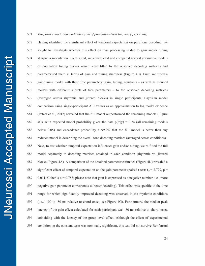
Temporal expectation modulates gain of population-level frequency processing 571
Having identified the significant effect of temporal expectation on pure tone decoding, we 572
sought to investigate whether this effect on tone processing is due to gain and/or tuning 573
sharpness modulation. To this end, we constructed and compared several alternative models 574
of population tuning curves which were fitted to the observed decoding matrices and 575
parameterised them in terms of gain and tuning sharpness (Figure 4B). First, we fitted a 576
gain/tuning model with three free parameters (gain, tuning, constant) – as well as reduced 577
models with different subsets of free parameters – to the observed decoding matrices 578
(averaged across rhythmic and jittered blocks) in single participants. Bayesian model 579
comparison using single-participant AIC values as an approximation to log model evidence 580
(Peters et al., 2012) revealed that the full model outperformed the remaining models (Figure 581
4C), with expected model probability given the data p(m|y) = 0.74 (all remaining models 582
below 0.05) and exceedance probability > 99.9% that the full model is better than any 583
reduced model in describing the overall tone decoding matrices (averaged across conditions). 584
Next, to test whether temporal expectation influences gain and/or tuning, we re-fitted the full 585
model separately to decoding matrices obtained in each condition (rhythmic vs. jittered 586
blocks; Figure 4A). A comparison of the obtained parameter estimates (Figure 4D) revealed a 587
significant effect of temporal expectation on the gain parameter (paired t-test: t21=-2.779, p = 588
0.011; Cohen’s d = 0.783; please note that gain is expressed as a negative number, i.e., more 589
negative gain parameter corresponds to better decoding). This effect was specific to the time 590
range for which significantly improved decoding was observed in the rhythmic conditions 591
(i.e., -100 to -80 ms relative to chord onset; see Figure 4G). Furthermore, the median peak 592
latency of the gain effect calculated for each participant was -80 ms relative to chord onset, 593
coinciding with the latency of the group-level effect. Although the effect of experimental 594
condition on the constant term was nominally significant, this test did not survive Bonferroni 595
25
correction for multiple comparisons (t21=2.101, p = 0.048). The effect of rhythm on the 596
tuning sharpness parameter was not significant (t21=1.039, p = 0.310). 597
Further, we tested whether the effect of temporal expectation on the gain parameter might be 598
driven by a specific class of tone frequencies, such as those discriminating between the two 599
chords that needed to be categorised by the participants. Thus, we repeated the model fitting 600
for four classes of tones (discriminant, adjacent, distant, and common frequencies; see 601
Methods for details). A repeated-measures ANOVA revealed a main effect of temporal 602
expectation, as identified above (F1,63 = 10.111, p = 0.004), but no main effect of frequency 603
type (F3,63 = 2.253, p = 0.091) and crucially no interaction between the two (F3,63 = 1.725, p = 604
0.171). Therefore, the effect of temporal expectation on gain did not depend on tone type 605
(Figure 4F). 606
Finally, we investigated whether the neural and behavioural benefits of temporal expectation 607
are correlated. Across participants, we correlated the z-scored differences between estimates 608
of the following variables, obtained from the rhythmic and jittered condition respectively: (1) 609
gain parameter, (2) tone decoding (i.e., rank-order correlation with the ideal decoding 610
matrix), (3) chord decoding (Mahalanobis distance), (4) behavioural accuracy. A significant 611
correlation was observed between the effect of temporal expectation on the gain parameter 612
and the underlying tone decoding modulation by temporal expectation (r = -.549, p = 0.008; 613
significant after Bonferroni-correcting for multiple comparisons across pairs of variables; 614
Figure 4E). After removing one outlier participants whose data were characterised by the 615
Cook’s distance metric exceeding the mean, the correlation remained significant: r = -.511, p 616
= 0.018). No other correlations were found to be significant. 617
618
DISCUSSION 619
620
26
We have shown that rhythmic temporal expectation improves target chord 621
discrimination accuracy, increases the phase-locking of neural signals at chord onset, as well 622
as improves M/EEG-based chord decoding. Interestingly, we also show that prior to chord 623
(i.e., a potential target) onset, temporal expectation improves decoding of irrelevant 624
distractors (pure tones). This beneficial effect can be modelled as increased gain to any 625
stimuli (auditory frequencies) presented at time points adjacent to expected chord onset, and 626
independent of whether processing these frequencies may be beneficial for chord 627
discrimination. 628
In the present study, rhythm-induced temporal expectation increased the participants’ 629
sensitivity to target chords. Similar behavioural improvements have been reported previously, 630
typically accompanied by shorter RTs to expected targets (Jaramillo and Zador, 2011; 631
Rimmele et al., 2011; Rohenkohl et al., 2012; Cravo et al., 2013). While here we only 632
compared responses to stimuli presented in rhythmic (isochronous) and jittered sequences 633
while controlling for physical differences between conditions (i.e., only selecting targets 634
preceded by identical intervals), other researchers have also found accuracy improvements in 635
quasi-rhythmic sequences when acoustic targets were presented following a mean interval vs. 636
at other intervals (Herrmann et al., 2016; see also Jones, 2015). Another recent study has 637
shown that, while different types of temporal expectation might lead to accuracy benefits, 638
rhythmic expectation specifically shortens RTs (Morillon et al., 2016). However, RTs have 639
been suggested to be more sensitive to temporal orienting in detection tasks than in 640
discrimination tasks (Correa et al., 2004). While in the present study participants were 641
instructed to discriminate chords by responding as soon as possible after hearing a target, 642
auditory streams continued for several hundreds of milliseconds following target offset, 643
which may have resulted in overall slow responses (Figure 1E) and a reduced sensitivity to 644
detect RT effects. 645
27
Beyond the increased behavioural sensitivity to target chords, we also observed 646
improved neural decoding of short chords in the rhythmic vs. jittered condition. Previous 647
auditory studies have shown that rhythmic presentation of targets presented at a low signal-648
to-noise ratio amid continuous distractors increases their detectability (Lawrance et al., 2014; 649
Rajendran et al., 2016). Similar findings in visual studies (ten Oever et al., 2017) have been 650
linked to increased phase-locking of neural activity around the expected target onset. In our 651
study rhythm-induced temporal expectation increased phase-locking of M/EEG signals at the 652
chord presentation rate (but not chord-evoked ERF/ERP amplitude), consistent with previous 653
reports (Cravo et al., 2013; Henry et al., 2014; Costa-Faidella et al. 2017) and with the 654
entrainment hypothesis (Schroeder & Lakatos, 2009; for a recent review, see: Haegens & 655
Zion-Golumbic, 2018), which posits that external rhythms synchronise low-frequency neural 656
activity and create time windows of increased sensitivity to stimuli presented at expected 657
latencies. However, since phase-locking has been shown to also increase due to interval-658
based expectations (Breska & Deouell), it may not be a specific measure of rhythm-induced 659
temporal expectation. 660
In addition to improving the decoding of short chords (potential targets), rhythmic 661
expectation also improved the decoding of pure tones (irrelevant distractors) preceding the 662
chords. Current hypotheses are largely agnostic to whether neural alignment to external 663
rhythms also results in temporal trade-offs, creating windows of decreased sensitivity at 664
unexpected or irrelevant latencies. Such competitive effects have been described in the 665
domain of spatial visual attention (Carrasco, 2011); however, temporal expectations have 666
been suggested to play a largely modulatory role, amplifying the influence of other (e.g. 667
spatial) sources of top-down control rather than themselves exerting strong influences on 668
neural processing (Rohenkohl et al., 2014). While processing limitations over time have long 669
been established – e.g., in the attentional blink literature (Shapiro, Raymond & Arnell, 1994) 670
28
– temporal expectations can in fact prevent attentional blink: knowing when subsequent 671
targets will occur can improve their processing and diminish the (detrimental) effects of 672
preceding targets (Martens & Johnson, 2005). Similarly, cues predicting target latency do 673
seem not only to improve target processing but also to impair processing targets that appear 674
at invalidly cued latencies (Denison et al., 2017). In this study, however, we did not observe 675
impaired processing of stimuli presented at unexpected time points, which would likely 676
manifest as impaired decoding and lower gain in the rhythmic vs. jittered condition several 677
hundred milliseconds before and after chord onset. Instead, our results suggest that while 678
rhythmic auditory expectation increases sensitivity at expected latencies, it does not 679
necessarily involve temporal trade-off with unexpected latencies. 680
We also considered another possible trade-off, namely temporal expectation boosting 681
the processing of relevant targets at the expense of irrelevant distractors. A recent EEG study 682
showed that anticipatory cues not only boost visual target decoding, but also decrease its 683
interference by distractors presented just after the targets, possibly reflecting a protective time 684
window for target processing (van Ede et al., 2018). However, as shown in other contexts 685
(Rohenkohl et al., 2011; Morillon et al., 2016; Breska & Ivry, 2018), rhythm-induced 686
expectations may not operate in the same manner as cue-induced expectations. Indeed, 687
rhythms can facilitate performance independently of whether they are predictive of when the 688
relevant targets may appear (Sanabria et al., 2011). In some cases, performance is superior for 689
those targets that occur on-beat, even if targets more often occur off-beat (Breska & Deouell, 690
2014). In line with the latter results, our findings show improved decoding of irrelevant 691
stimuli if they are presented at latencies leading up to the expected onsets of potential targets. 692
While these differences were observed between -100 and -80 ms but not at even shorter 693
latencies prior to chord onset, it is worth noting that decoding pure tones was based on 694
M/EEG activity evoked by these tones (i.e., with a lag of up to 126 ms). Thus, just before 695
29
chord onset, interference between chord-evoked activity and tone-evoked activity may have 696
compromised tone decoding. Given the previously observed differences between rhythm- and 697
cue-induced temporal expectations, it remains an important open question whether the type of 698
temporal expectation manipulations, and/or individual participants’ strategies in generating 699
these expectations, may influence the latencies at which improved decoding can be observed. 700
To interpret the finding that rhythm-based expectation improves decoding of 701
irrelevant distractors prior to the expected target onset, we used a model which independently 702
parameterised the gain and tuning of population-level frequency coding and found that 703
rhythm-based expectation increased the gain of pure tone decoding. No evidence was found 704
for the sharpening of tuning induced by temporal expectation. This suggests that, unlike in 705
previous (animal) studies showing that sustained attention to acoustic rhythms (O’Connell et 706
al., 2014) or increased target onset probability (Jaramillo & Zador, 2011) sharpen frequency 707
tuning, in the current study rhythm-induced expectations – at the level of population-based 708
decoding – could be linked to dynamic modulations of gain, more akin to classical 709
neuromodulatory effects (Auksztulewicz et al., 2018). Previous behavioural modelling 710
studies showed that rhythm-based expectation does indeed increase the signal-to-noise gain 711
of sensory evidence in a visual discrimination task (Rohenkohl et al., 2012). Here, the gain 712
effect was independent of whether the specific frequencies were useful for discriminating 713
potential targets, further supporting the notion that the rhythmic increases of sensitivity are 714
independent of stimulus relevance (Breska & Deouell, 2014). It is worth noting that unlike in 715
the previous electrophysiology studies (Lakatos et al., 2013; O’Connell et al., 2014), the 716
perceptual discriminations here were based on chords with no overall frequency differences - 717
showing that rhythm-induced expectations can work on composite representations. It remains 718
to be tested whether the rhythm-induced dynamic gain modulation generalizes across data 719
modalities and species (e.g., invasive recordings in animal models). 720
30
On a methodological note, our study is the first to show robust M/EEG-based 721
multivariate decoding of pure tone frequency across a broad range of frequencies. While 722
recent studies have brought substantial advances in decoding auditory features, studies using 723
discreet stimuli have focused on decoding complex features such as pitch/rate modulation 724
based on spectral information in MEG signals (Herrmann et al., 2013b), or bistable percepts 725
based on evoked MEG responses (Billig et al., 2018). In the domain of speech decoding, 726
speech-evoked responses can be used to decode vowel categories (Yi et al., 2017) but 727
typically a combination of complex spectral features is used to decode speech envelope (Luo 728
& Poeppel, 2007; Ng et al., 2013; de Cheveigne et al., 2018). Here, robust decoding of pure 729
tone frequency was achieved based on relatively early M/EEG- response latencies (<100 ms) 730
evoked by very brief tones (~33 ms), despite their presentation in gapless streams. Finally, 731
topographies of correlations between M/EEG amplitudes and tone frequency could be 732
localised to auditory regions, suggesting that frequency decoding is based on sensory 733
processing of acoustic features rather than on hierarchically higher activity related to complex 734
percepts. 735
In summary, we have demonstrated that rhythmic expectation enhances population 736
responses not only to task-relevant targets, but also to task-irrelevant distractors preceding 737
potential targets. The latter effect could be explained in terms of non-specific neural gain 738
changes at time points adjacent to rhythm-induced expectation of relevant latencies. These 739
findings speak against necessary temporal trade-offs in rhythmic orienting and support 740
theories of neural alignment to the rhythmic structure of stimulus streams, plausibly mediated 741
by dynamic neuromodulation. 742
743
REFERENCES 744
745
31
Auksztulewicz R, Schwiedrzik CM, Thesen T, Doyle W, Devinsky O, Nobre AC, Schroeder 746
CE, Friston KJ, Melloni L (2018) Not All Predictions Are Equal: "What" and "When" 747
Predictions Modulate Activity in Auditory Cortex through Different Mechanisms. J 748
Neurosci. 38(40):8680-8693. 749
Billig AJ, Davis MH, Carlyon RP (2018) Neural Decoding of Bistable Sounds Reveals an 750
Effect of Intention on Perceptual Organization. J Neurosci. 38(11):2844-2853. 751
Bobadilla-Suarez S, Ahlheim C, Mehrotra A, Panos A, Love BC (2019) Measures of neural 752
similarity. BioRxiv, doi: 10.1101/439893. 753
Breska A, Deouell LY (2017) Neural mechanisms of rhythm-based temporal prediction: 754
Delta phase-locking reflects temporal predictability but not rhythmic entrainment. PLoS 755
Biol. 15(2):e2001665. 756
Breska A, Deouell LY (2014) Automatic bias of temporal expectations following temporally 757
regular input independently of high-level temporal expectation. J Cogn Neurosci. 26:1555-758
1571. 759
Breska A, Ivry RB (2018) Double dissociation of single-interval and rhythmic temporal 760
prediction in cerebellar degeneration and Parkinson’s disease. PNAS. 115(48):12283-761
12288. 762
Carrasco M (2011) Visual attention: The past 25 years. Vision Research. 51(13):1484–1525. 763
Cornelissen FW, Peters EM, Palmer J (2002) The Eyelink Toolbox: eye tracking with 764
MATLAB and the Psychophysics Toolbox. Behav Res Methods Instrum Comput. 765
34(4):613-7. 766
Correa A, Lupiáñez J, Milliken B, Tudela P (2004) Endogenous temporal orienting of 767
attention in detection and discrimination tasks. Percept Psychophys. 66(2):264-78. 768
Costa-Faidella J, Sussman ES, Escera C (2017) Selective entrainment of brain oscillations 769
drives auditory perceptual organization. Neuroimage. 159:195-206. 770
32
Cravo AM, Rohenkohl G, Wyart V, Nobre AC (2013) Temporal expectation enhances 771
contrast sensitivity by phase entrainment of low-frequency oscillations in visual cortex. J 772
Neurosci. 33(9):4002-10. 773
de Cheveigné A, Wong DDE, Di Liberto GM, Hjortkjær J, Slaney M, Lalor E (2018) 774
Decoding the auditory brain with canonical component analysis. Neuroimage. 172:206-775
216. 776
De Maesschalck R, Jouan-Rimbaud D, Massart DL (2000) The Mahalanobis 777
distance. Chemom Intell Lab Syst. 50:1–18. 778
Denison RN, Heeger DJ, Carrasco M (2017) Attention flexibly trades off across points in 779
time. Psychon Bull Rev. 24(4):1142-1151. 780
Garcia JO, Srinivasan R, Serences JT (2013) Near-real-time feature-selective modulations in 781
human cortex. Curr Biol. 23(6):515-22. 782
Glasberg BR, Moore BCJ (2002) A model of loudness applicable to time-varying sounds. J 783
Audio Eng Soc. 50(5):331-342. 784
Grootswagers T, Wardle SG, Carlson TA (2017) Decoding dynamic brain patterns from 785
evoked responses: a tutorial on multivariate pattern analysis applied to time series 786
neuroimaging data. J Cogn Neurosci 29(4):677-697. 787
Guggenmos M, Sterzer P, Cichy RM (2018) Multivariate pattern analysis for MEG: a 788
comparison of dissimilarity measures. Neuroimage 173:434-447. 789
Haegens S, Zion Golumbic E (2018) Rhythmic facilitation of sensory processing: A critical 790
review. Neurosci Biobehav Rev. 86:150-165. 791
Henry MJ, Herrmann B, Obleser J (2014) Entrained neural oscillations in multiple frequency 792
bands comodulate behavior. PNAS. 111(41):14935-40. 793
Henson RN, Mouchlianitis E, Friston KJ (2009) MEG and EEG data fusion: Simultaneous 794
localisation o face-evoked responses. Neuroimage 47:581-589. 795
33
Herrmann B, Henry MJ, Obleser J (2013a) Frequency-specific adaptation in human auditory 796
cortex depends on the spectral variance in the acoustic stimulation. J Neurophysiol 797
109:2086-2096. 798
Herrmann B, Henry MJ, Grigutsch M, Obleser J (2013b) Oscillatory phase dynamics in 799
neural entrainment underpin illusory percepts of time. J Neurosci. 33(40):15799-809. 800
Herrmann B, Henry MJ, Haegens S, Obleser J (2016) Temporal expectations and neural 801
amplitude fluctuations in auditory cortex interactively influence perception. Neuroimage 802
124:487-497. 803
Ille N, Berg P, Scherg M (2002) Artifact correction of the ongoing EEG using spatial filters 804
based on artefact and brain signal topographies. J Clin Neurophysiol. 19, 113–124. 805
Jaramillo S, Zador AM (2011) The auditory cortex mediates the perceptual effects of acoustic 806
temporal expectation. Nat Neurosci. 14(2):246-51. 807
Jones A (2015) Independent effects of bottom-up temporal expectancy and top-down spatial 808
attention. An audiovisual study using rhythmic cueing. Front Integr Neurosci 8:96. 809
Kilner JM, Kiebel SJ, Friston KJ (2005) Applications of random field theory to 810
electrophysiology. Neurosci Lett. 374:174 –178. 811
Kriegeskorte N, Douglas PK (2019) Interpreting encoding and decoding models. Current 812
Opinion in Neurobiology, 55:167-179. 813
Lachaux JP, Rodriguez E, Martinerie J, Varela FJ (1999) Measuring phase synchrony in brain 814
signals. Hum Brain Mapp. 8(4):194-208. 815
Lakatos P, Karmos G, Mehta AD, Ulbert I, Schroeder CE (2008) Entrainment of neuronal 816
oscillations as a mechanism of attentional selection. Science. 320(5872):110-3. 817
Lakatos P, Musacchia G, O’Connel MN, Falchier AY, Javitt DC, Schroeder CE (2013) The 818
spectrotemporal filter mechanism of auditory selective attention. Neuron. 77(4):750-761. 819
34
Lawrance EL, Harper NS, Cooke JE, Schnupp JW (2014) Temporal predictability enhances 820
auditory detection. J Acoust Soc Am. 135(6):EL357-63. 821
Ledoit O, Wolf M (2004) Honey, I shrunk the sample covariance matrix. J Portf Manag. 822
30:110–119. 823
Ling S, Liu T, Carrasco M (2009) How spatial and feature-based attention affect the gain and 824
tuning of population responses. Vision research. 49(10):1194-1204. 825
Litvak V, Friston K (2008) Electromagnetic source reconstruction for group studies. 826
Neuroimage 42:1490-1498. 827
López JD, Litvak V, Espinosa JJ, Friston K, Barnes GR (2014) Algorithmic procedures for 828
Bayesian MEG/EEG source reconstruction in SPM. Neuroimage 84:476-487. 829
Luo H, Poeppel D (2007) Phase patterns of neuronal responses reliably discriminate speech 830
in human auditory cortex. Neuron. 54(6):1001-10. 831
Maris E, Oostenveld R (2007) Nonparametric statistical testing of EEG- and MEG-data. J 832
Neurosci Methods. 164(1):177-90. 833
Martens S, Johnson A (2005) Timing attention: cuing target onset interval attenuates the 834
attentional blink. Mem Cognit. 33(2):234-40. 835
Miller LM, Escabi MA, Read HL, Schreiner CE (2002) Spectrotemporal receptive fields in 836
the lemniscal auditory thalamus and cortex. J Neurophysiol. 87(1):516-527. 837
Morillon B, Schroeder CE, Wyart V, Arnal LH (2016) Temporal Prediction in lieu of 838
Periodic Stimulation. J Neurosci. 36(8):2342-7. 839
Myers NE, Rohenkohl G, Wyart V, Woolrich MW, Nobre AC, Stokes MG (2015) Testing 840
sensory evidence against mnemonic templates. Elife. 4:e09000. 841
Ng BS, Logothetis NK, Kayser C (2013) EEG phase patterns reflect the selectivity of neural 842
firing. Cereb Cortex. 23(2):389-98. 843
35
Nobre AC, van Ede F (2018) Anticipated moments: temporal structure in attention. Nat Rev 844
Neurosci. 19(1):34-48. 845
O'Connell MN, Barczak A, Schroeder CE, Lakatos P (2014) Layer specific sharpening of 846
frequency tuning by selective attention in primary auditory cortex. J Neurosci. 847
34(49):16496-508. 848
Obleser J, Henry MJ, Lakatos P (2017) What do we talk about when we talk about rhythm? 849
Plos Biol 15(11):e1002615. 850
Peters J, Miedl SF, Büchel C (2012) Formal comparison of dual-parameter temporal 851
discounting models in controls and pathological gamblers. PLoS One. 7(11):e47225. 852
Picton TW, Woods DL, Proulx GB (1978) Human auditory sustained potentials. II. Stimulus 853
relationships. Electroencephalography and Clinical Neurophysiology 45:198-210. 854
Praamstra P, Kourtis D, Kwok HF, Oostenveld R (2006) Neurophysiology of implicit timing 855
in serial choice reaction-time performance. J Neurosci. 26(20):5448-55. 856
Rajendran VG, Harper NS, Abdel-Latif KH, Schnupp JW (2016) Rhythm Facilitates the 857
Detection of Repeating Sound Patterns. Front Neurosci. 10:9. 858
Rimmele J, Jolsvai H, Sussman E (2011) Auditory target detection is affected by implicit 859
temporal and spatial expectations. J Cogn Neurosci. 23(5):1136-47. 860
Rohenkohl G, Coull JT, Nobre AC (2011) Behavioural dissociation between exogenous and 861
endogenous temporal orienting of attention. PLoS One. 6(1):e14620. 862
Rohenkohl G, Nobre AC (2011) α oscillations related to anticipatory attention follow 863
temporal expectations. J Neurosci. 31(40):14076-84. 864
Rohenkohl G, Cravo AM, Wyart V, Nobre AC (2012) Temporal expectation improves the 865
quality of sensory information. J Neurosci. 32(24):8424-8428. 866
Rohenkohl G, Gould IC, Pessoa J, Nobre AC (2014) Combining spatial and temporal 867
expectations to improve visual perception. J Vis. 14(4):8. 868
36
Sanabria D, Capizzi M, Correa A (2011) Rhythms that speed you up. J Exp Psychol Hum 869
Percept Perform. 37:236–244. 870
Schroeder CE, Lakatos P (2009) Low-frequency neuronal oscillations as instruments of 871
sensory selection. Trends Neurosci. 32: 9–18. 872
Shapiro KL, Raymond JE, Arnell KM (1994) Attention to visual pattern information 873
produces the attentional blink in rapid serial visual presentation. J Exp Psychol Hum 874
Percept Perform. 20(2):357-71. 875
Stefanics G, Hangya B, Hernádi I, Winkler I, Lakatos P, Ulbert I (2010) Phase entrainment of 876
human delta oscillations can mediate the effects of expectation on reaction speed. J 877
Neurosci. 30(41):13578-85. 878
Su L, Zulfigar I, Jamshed F, Fonteneau E, Marslen-Wilson W (2014) Mapping tonotopic 879
organization in human temporal cortex: representational similarity analysis in EMEG 880
source space. Front Neurosci 8:368. 881
Tabachnick AR, Toscano JC (2018) Perceptual encoding in auditory brainstem responses: 882
effects of stimulus frequency. Journal of Speech, Language, and Hearing Research 883
61:2364-2375. 884
ten Oever S, Schroeder CE, Poeppel D, van Atteveldt N, Mehta AD, Mégevand P, Groppe 885
DM, Zion-Golumbic E (2017) Low-Frequency Cortical Oscillations Entrain to 886
Subthreshold Rhythmic Auditory Stimuli. J Neurosci. 37(19):4903-4912. 887
Van Diepen RM, Mazaheri A (2018) The caveats of observing inter-trial phase-coherence in 888
cognitive neuroscience. Sci Rep 8:2990. 889
van Ede F, Chekroud SR, Stokes MG, Nobre AC (2018) Decoding the influence of 890
anticipatory states on visual perception in the presence of temporal distractors. Nat 891
Commun. 9(1):1449. 892
37
Walther A, Nili H, Ejaz N, Alink A, Kriegeskorte N, Diedrichsen J (2016) Reliability of 893
dissimilarity measures for multi-voxel pattern analysis. Neuroimage 137:188-200. 894
Wolff MJ, Jochim J, Akyürek EG, Stokes MG (2017) Dynamic hidden states underlying 895
working-memory-guided behavior. Nature neuroscience. 20(6):864-871. 896
Woods DL, Alain C, Covarrubias D, Zaidel O (1995) Middle latency auditory evoked 897
potentials to tones of different frequency. Hear Res. 85(1-2):69-75. 898
Yi HG, Xie Z, Reetzke R, Dimakis AG, Chandrasekaran B (2017) Vowel decoding from 899
single-trial speech-evoked electrophysiological responses: A feature-based machine 900
learning approach. Brain and behaviour. 7(6):e00665. 901
Zanto TP, Pan P, Liu H, Bollinger J, Nobre AC, Gazzaley A (2011) Age-related changes in 902
orienting attention in time. J Neurosci. 31(35):12461-70. 903
Zoefel B, VanRullen R (2017) Oscillatory Mechanisms of Stimulus Processing and Selection 904
in the Visual and Auditory Systems: State-of-the-Art, Speculations and Suggestions. Front 905
Neurosci 11:296. 906
907
908
909
910
911
912
913
914
915
916
917
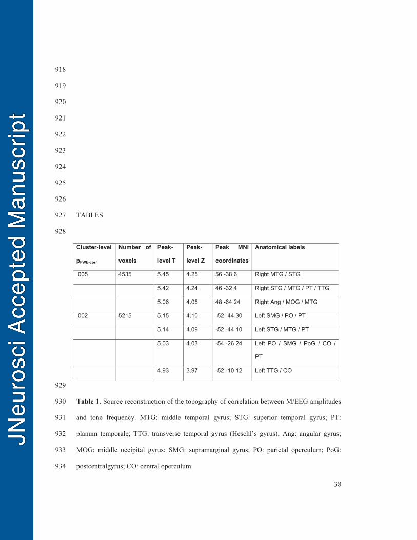
38
918
919
920
921
922
923
924
925
926
TABLES 927
928
Cluster-level
pFWE-corr
Number of
voxels
Peak-
level T
Peak-
level Z
Peak MNI
coordinates
Anatomical labels
.005 4535 5.45 4.25 56 -38 6 Right MTG / STG
5.42 4.24 46 -32 4 Right STG / MTG / PT / TTG
5.06 4.05 48 -64 24 Right Ang / MOG / MTG
.002 5215 5.15 4.10 -52 -44 30 Left SMG / PO / PT
5.14 4.09 -52 -44 10 Left STG / MTG / PT
5.03 4.03 -54 -26 24 Left PO / SMG / PoG / CO /
PT
4.93 3.97 -52 -10 12 Left TTG / CO
929
Table 1. Source reconstruction of the topography of correlation between M/EEG amplitudes 930
and tone frequency. MTG: middle temporal gyrus; STG: superior temporal gyrus; PT: 931
planum temporale; TTG: transverse temporal gyrus (Heschl’s gyrus); Ang: angular gyrus; 932
MOG: middle occipital gyrus; SMG: supramarginal gyrus; PO: parietal operculum; PoG: 933
postcentralgyrus; CO: central operculum 934
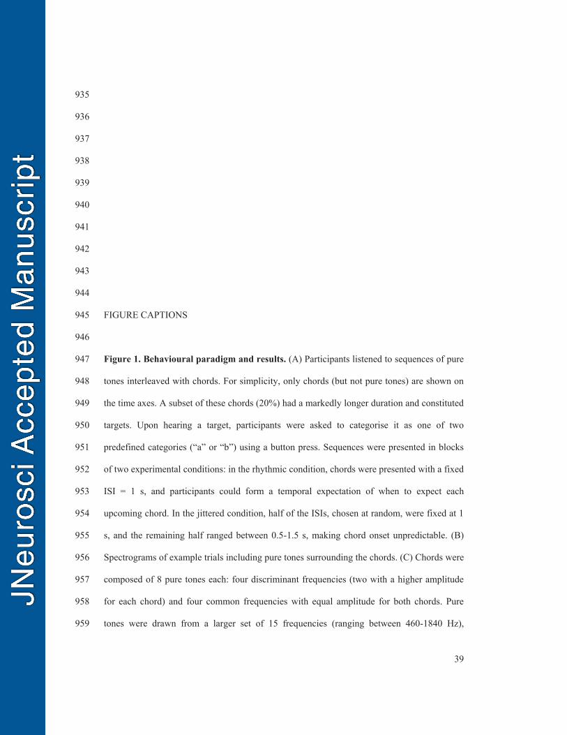
39
935
936
937
938
939
940
941
942
943
944
FIGURE CAPTIONS 945
946
Figure 1. Behavioural paradigm and results. (A) Participants listened to sequences of pure 947
tones interleaved with chords. For simplicity, only chords (but not pure tones) are shown on 948
the time axes. A subset of these chords (20%) had a markedly longer duration and constituted 949
targets. Upon hearing a target, participants were asked to categorise it as one of two 950
predefined categories (“a” or “b”) using a button press. Sequences were presented in blocks 951
of two experimental conditions: in the rhythmic condition, chords were presented with a fixed 952
ISI = 1 s, and participants could form a temporal expectation of when to expect each 953
upcoming chord. In the jittered condition, half of the ISIs, chosen at random, were fixed at 1 954
s, and the remaining half ranged between 0.5-1.5 s, making chord onset unpredictable. (B) 955
Spectrograms of example trials including pure tones surrounding the chords. (C) Chords were 956
composed of 8 pure tones each: four discriminant frequencies (two with a higher amplitude 957
for each chord) and four common frequencies with equal amplitude for both chords. Pure 958
tones were drawn from a larger set of 15 frequencies (ranging between 460-1840 Hz), 959
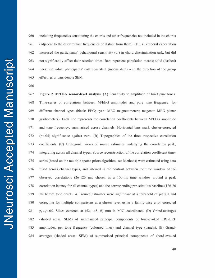
40
including frequencies constituting the chords and other frequencies not included in the chords 960
(adjacent to the discriminant frequencies or distant from them). (D,E) Temporal expectation 961
increased the participants’ behavioural sensitivity (d’) in chord discrimination task, but did 962
not significantly affect their reaction times. Bars represent population means; solid (dashed) 963
lines: individual participants’ data consistent (inconsistent) with the direction of the group 964
effect; error bars denote SEM. 965
966
Figure 2. M/EEG sensor-level analysis. (A) Sensitivity to amplitude of brief pure tones. 967
Time-series of correlations between M/EEG amplitudes and pure tone frequency, for 968
different channel types (black: EEG; cyan: MEG magnetometers; magenta: MEG planar 969
gradiometers). Each line represents the correlation coefficients between M/EEG amplitude 970
and tone frequency, summarised across channels. Horizontal bars mark cluster-corrected 971
(p<.05) significance against zero. (B) Topographies of the three respective correlation 972
coefficients. (C) Orthogonal views of source estimates underlying the correlation peak, 973
integrating across all channel types. Source reconstruction of the correlation coefficient time-974
series (based on the multiple sparse priors algorithm; see Methods) were estimated using data 975
fused across channel types, and inferred in the contrast between the time window of the 976
observed correlations (26-126 ms; chosen as a 100-ms time window around a peak 977
correlation latency for all channel types) and the corresponding pre-stimulus baseline (126-26 978
ms before tone onset). All source estimates were significant at a threshold of p<.001 and 979
correcting for multiple comparisons at a cluster level using a family-wise error corrected 980
pFWE<.05. Slices centered at (52, -48, 6) mm in MNI coordinates. (D) Grand-averages 981
(shaded areas: SEM) of summarised principal components of tone-evoked ERP/ERF 982
amplitudes, per tone frequency (coloured lines) and channel type (panels). (E) Grand-983
averages (shaded areas: SEM) of summarised principal components of chord-evoked 984
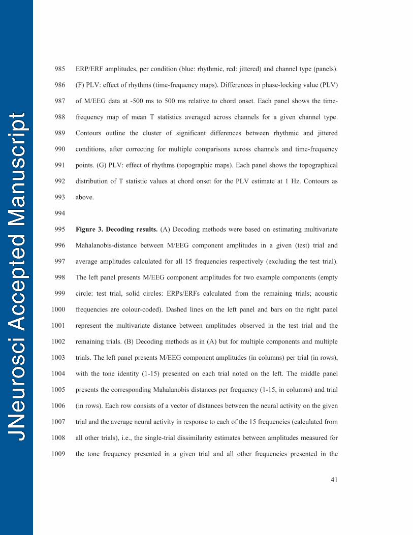
41
ERP/ERF amplitudes, per condition (blue: rhythmic, red: jittered) and channel type (panels). 985
(F) PLV: effect of rhythms (time-frequency maps). Differences in phase-locking value (PLV) 986
of M/EEG data at -500 ms to 500 ms relative to chord onset. Each panel shows the time-987
frequency map of mean T statistics averaged across channels for a given channel type. 988
Contours outline the cluster of significant differences between rhythmic and jittered 989
conditions, after correcting for multiple comparisons across channels and time-frequency 990
points. (G) PLV: effect of rhythms (topographic maps). Each panel shows the topographical 991
distribution of T statistic values at chord onset for the PLV estimate at 1 Hz. Contours as 992
above. 993
994
Figure 3. Decoding results. (A) Decoding methods were based on estimating multivariate 995
Mahalanobis-distance between M/EEG component amplitudes in a given (test) trial and 996
average amplitudes calculated for all 15 frequencies respectively (excluding the test trial). 997
The left panel presents M/EEG component amplitudes for two example components (empty 998
circle: test trial, solid circles: ERPs/ERFs calculated from the remaining trials; acoustic 999
frequencies are colour-coded). Dashed lines on the left panel and bars on the right panel 1000
represent the multivariate distance between amplitudes observed in the test trial and the 1001
remaining trials. (B) Decoding methods as in (A) but for multiple components and multiple 1002
trials. The left panel presents M/EEG component amplitudes (in columns) per trial (in rows), 1003
with the tone identity (1-15) presented on each trial noted on the left. The middle panel 1004
presents the corresponding Mahalanobis distances per frequency (1-15, in columns) and trial 1005
(in rows). Each row consists of a vector of distances between the neural activity on the given 1006
trial and the average neural activity in response to each of the 15 frequencies (calculated from 1007
all other trials), i.e., the single-trial dissimilarity estimates between amplitudes measured for 1008
the tone frequency presented in a given trial and all other frequencies presented in the 1009
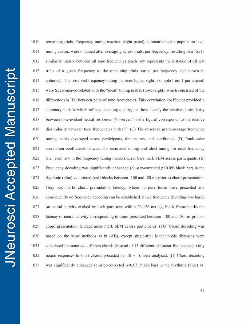
42
remaining trials. Frequency tuning matrices (right panel), summarising the population-level 1010
tuning curves, were obtained after averaging across trials, per frequency, resulting in a 15x15 1011
similarity matrix between all tone frequencies (each row represents the distance of all test 1012
trials of a given frequency to the remaining trials sorted per frequency and shown in 1013
columns). The observed frequency tuning matrices (upper right: example from 1 participant) 1014
were Spearman-correlated with the “ideal” tuning matrix (lower right), which consisted of the 1015
difference (in Hz) between pairs of tone frequencies. This correlation coefficient provided a 1016
summary statistic which reflects decoding quality, i.e., how closely the relative dissimilarity 1017
between tone-evoked neural responses (‘observed’ in the figure) corresponds to the relative 1018
dissimilarity between tone frequencies (‘ideal’). (C) The observed grand-average frequency 1019
tuning matrix (averaged across participants, time points, and conditions). (D) Rank-order 1020
correlation coefficients between the estimated tuning and ideal tuning for each frequency 1021
(i.e., each row in the frequency tuning matrix). Error bars mark SEM across participants. (E) 1022
Frequency decoding was significantly enhanced (cluster-corrected p<0.05; black bar) in the 1023
rhythmic (blue) vs. jittered (red) blocks between -100 and -80 ms prior to chord presentation. 1024
Grey box marks chord presentation latency, where no pure tones were presented and 1025
consequently no frequency decoding can be established. Since frequency decoding was based 1026
on neural activity evoked by each pure tone with a 26-126 ms lag, black frame marks the 1027
latency of neural activity corresponding to tones presented between -100 and -80 ms prior to 1028
chord presentation. Shaded areas mark SEM across participants. (FG) Chord decoding was 1029
based on the same methods as in (AB), except single-trial Mahalanobis distances were 1030
calculated for same vs. different chords (instead of 15 different distractor frequencies). Only 1031
neural responses to short chords preceded by ISI = 1s were analysed. (H) Chord decoding 1032
was significantly enhanced (cluster-corrected p<0.05; black bar) in the rhythmic (blue) vs. 1033
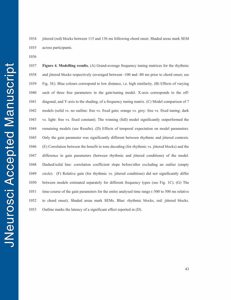
43
jittered (red) blocks between 115 and 136 ms following chord onset. Shaded areas mark SEM 1034
across participants. 1035
1036
Figure 4. Modelling results. (A) Grand-average frequency tuning matrices for the rhythmic 1037
and jittered blocks respectively (averaged between -100 and -80 ms prior to chord onset; see 1038
Fig. 3E). Blue colours correspond to low distance, i.e. high similarity. (B) Effects of varying 1039
each of three free parameters in the gain/tuning model. X-axis corresponds to the off-1040
diagonal, and Y-axis to the shading, of a frequency tuning matrix. (C) Model comparison of 7 1041
models (solid vs. no outline: free vs. fixed gain; orange vs. grey: free vs. fixed tuning; dark 1042
vs. light: free vs. fixed constant). The winning (full) model significantly outperformed the 1043
remaining models (see Results). (D) Effects of temporal expectation on model parameters. 1044
Only the gain parameter was significantly different between rhythmic and jittered contexts. 1045
(E) Correlation between the benefit in tone decoding (for rhythmic vs. jittered blocks) and the 1046
difference in gain parameters (between rhythmic and jittered conditions) of the model. 1047
Dashed/solid line: correlation coefficient slope before/after excluding an outlier (empty 1048
circle). (F) Relative gain (for rhythmic vs. jittered conditions) did not significantly differ 1049
between models estimated separately for different frequency types (see Fig. 1C). (G) The 1050
time-course of the gain parameters for the entire analysed time range (-500 to 500 ms relative 1051
to chord onset). Shaded areas mark SEMs. Blue: rhythmic blocks, red: jittered blocks. 1052
Outline marks the latency of a significant effect reported in (D). 1053
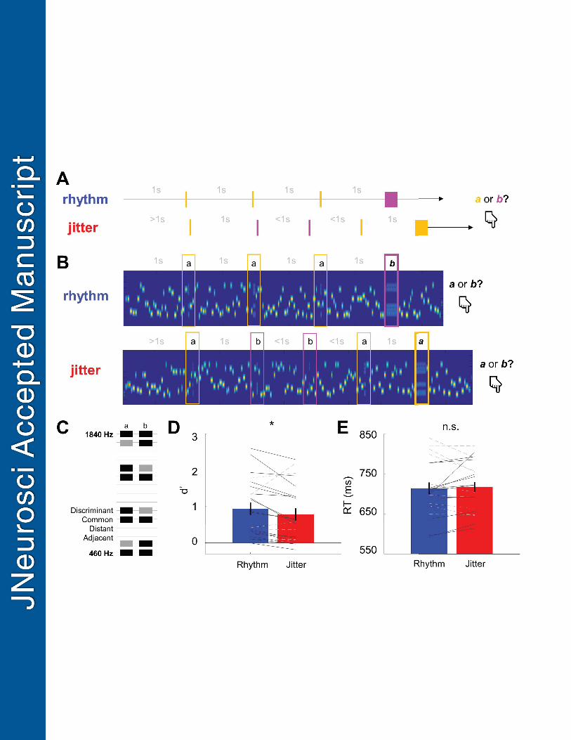
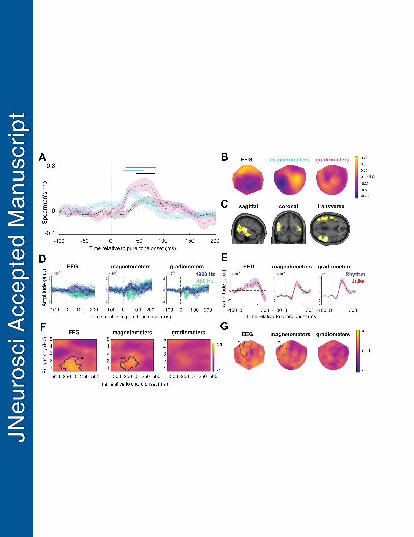
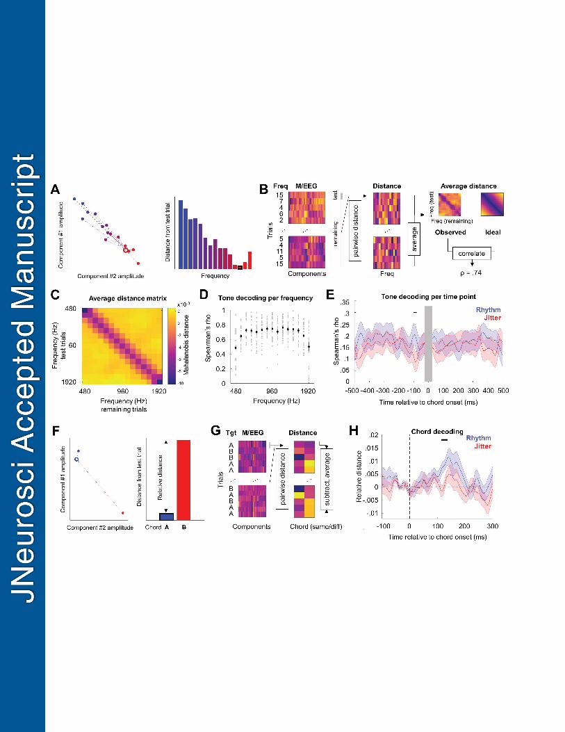
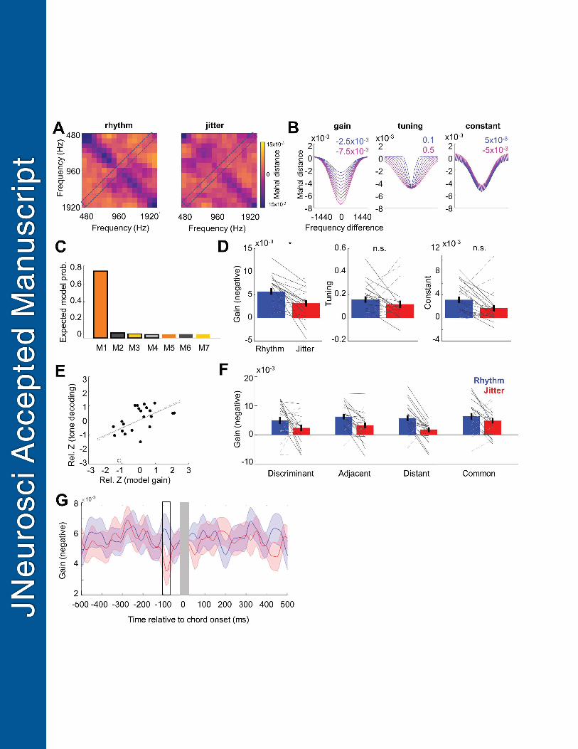
Related Documents