Rheo-optical response of carbon nanotube suspensions

1

Rheo-optical response of carbon nanotube suspensions

G. Natale a, N. K. Reddy b, G. Ausias c, J. Férec c, M.C. Heuzey a and P.J. Carreau a

a Research Center for High Performance Polymer and Composite Systems (CREPEC),

Chemical Engineering Department, Polytechnique Montreal,

PO Box 6079, Stn Centre-Ville, Montreal, QC, Canada H3C 3A7

b Department of Chemical Engineering, K.U. Leuven, W. de Croylaan 46, B-3001 Leuven,

Belgium

c

Univ. Bretagne-Sud, EA 4250, LIMATB, F-56100 Lorient, France

SYNOPSIS

In this work, the rheo-optical response of multi-walled carbon nanotube (MWCNT) suspensions

was analyzed. Dichroism was obtained using a polarization-modulation technique in parallel

disks and for the first time for these particles in a Couette flow geometry. MWCNTs were

dispersed in a Newtonian epoxy matrix, at different concentrations covering the dilute and semi-

dilute regimes. Measurements of dichroism were performed as functions of shear rate and

nanotube concentration. Surprisingly, the ultimate average orientation angle with respect to the

flow direction was far from zero degree, even at high Peclet (Pe) numbers in very dilute

suspensions. To explain this peculiar behavior, a new model for flexible rods, valid in the dilute

regime, is proposed. It is based on the development of Strautins and Latz (2007) that considers

flexible rods made of beads and connectors. We modified their bending potential that allows

only straight rods at equilibrium with a harmonic cosine expression. This simple modification

2

changes drastically the behavior of these flexible particles that exhibit a non negligible

orientation in the vorticity direction under steady state.

I. Introduction

The increasing demand for more efficient processing schemes for colloidal suspensions requires

a complete understanding of the fundamentals of their flow behavior. This knowledge can open

up new routes not only to optimize tools to control such processes, but also to tailor materials

based on predicted microstructure-macroscopic properties interplay. Colloidal suspensions of

highly anisotropic particles attract increasing interest because of the number of potential

applications, from organic electronics to micromechanics and composites. In this class of

particles, carbon nanotubes (CNTs) are fascinating because they exhibit features at the frontier

between a semi-flexible macromolecule and a micro-size fiber. Furthermore, their quasi-one-

dimensional structure gives them unique thermal and electrical properties that have made CNTs

the polymer filler of choice for the creation of multi functional composites [Du et al. (2004),

Abdel-Goad and Pötschke (2005), Hu et al. (2006)].

Many publications have recently appeared on the rheology of CNT suspensions. See for

examples Fan and Advani (2007) and Hobbie and Fry (2007). In small amplitude oscillatory

flows (SAOS), suspensions of unmodified CNTs exhibit mild elasticity (low values of ) at

very low concentration [Rahatekar et al. (2006), Ma et al. (2008)]. Crossing the limit of

percolation, the tube network contribution becomes predominant with the storage modulus, ,

that overcomes the loss counterpart, G . In addition, both moduli of percolated systems present a

non-terminal character at low frequencies [Abdel-Goad and Pötschke (2005), Hu et al. (2006)].

Percolation concentration thresholds are strongly dependent on the particle aspect ratio if well

dispersed systems are compared [Huang et al. (2006), Abbasi et al. (2009)]. Furthermore, the

3

moduli are functions of the thermo-mechanical history. Increasing pre-shearing intensity before

an SAOS test causes a reduction of that increases with time, indicative of a structure build up

until it reaches a new meta-stable equilibrium state [Khalkhal et al. (2011)]. The pre-shearing

step causes a destruction of the network by orienting the tubes in the flow direction. During rest

time, Brownian motion dominates, re-establishing the network by interlocking the tubes in a new

state. This evolution of the structure upon rest was also confirmed by transient tests consisting of

multiple shear start-ups spaced out with rest steps [Wu et al. (2007), Khalkhal and Carreau

(2012)]. Recently, Pujari et al. (2009) and (2011) linked directly microstructure and rheological

features by probing concentrated CNT suspensions by small- and wide-angle x-ray scattering

(SAXS and WAXS). The rheological and orientation data were discussed in terms of distortion,

breakdown, and reformation of percolated multi-walled carbon nanotube (MWCNT) networks.

Another rheological characteristic of CNT suspensions is their marked shear-thinning behavior

during steady shear rate ramp tests [Rahatekar et al. (2006)]. Non negligible first normal stress

difference, N1, was also reported in cone-and-plate flow rheometry [Natale et al. (2014)].

The optical contrast between CNTs and most typical polymers make CNT suspensions good

candidates to be probed with rheo-optical techniques, especially considering that these

suspensions exhibits reasonably strong anisotropy [Hobbie (2004)]. Rheo-optical techniques are

extremely useful to link in real time rheological information to microstructure evolution. In flow

dichroism and birefringence studies, the material property of interest is the refractive index

tensor, ' ''in n n . The real part of this tensor, 'n , causes the phase shift in the transmitted light

while the imaginary component, ''n , characterizes the attenuation. When the refractive index

tensor is anisotropic, the differences in the principal eigenvalues of its real 'n and imaginary

''n parts are defined as birefringence and dichroism, respectively. Following the approach of

4

Onuki and Doi (1986), Hobbie (2004) derived an expression for the dielectric tensor of CNT

suspensions valid in the dilute and semi-dilute regimes and as function of concentration, spatial

fluctuation and orientation of the rods.

The first published rheo-optical study of CNT suspensions was performed by Fry et al.

(2006). They studied single- and multi-walled CNTs suspended in various media using parallel

plate (disk) flow geometry. Their results were in qualitative agreement with the theoretical

predictions of Doi and Edwards (1986) at low Pe number, while at high Pe the degree of

nanotube alignment scaled with Pe1/6.

The Doi-Edwards model [Doi and Edwards (1978)] and his extension for polydisperse

systems called the DEMG model [Marrucci and Grizzuti (1983)] were used in the past to

describe the rheo-optical response of collagen proteins in transient flows [Chow et al. (1985a,

b)]. The DEMG model was able to account correctly for polydispersity of the aspect ratio of the

systems. However, the birefringence overshoots were always underestimated. This was mainly

attributed to the flexibility of the particles, which was not accounted for in the model.

An alternative approach to take into account flexibility was proposed by Strautins and

Latz (2007). Their model consists of a semi-flexible system of three beads and two connectors,

subjected to a bending potential. In their work, they allowed only small deviations from straight

rod conformation in order to obtain simple closures for the evolution equations of the second

order orientation tensors. For shear flow, this assumption results in a completely aligned system

in absence of Brownian motion while we would suspect flexibility to play an important role on

the final orientation of the system. Furthermore, the effects of the bending potential are important

only in flow fields where the second order derivative of the velocity is non zero. This implies

that for simple shear flow (or in general for many rheological flows), flexibility would not have

5

any effect in contrast with the experimental literature [Keshtkar et al. (2010)] and other models

for semi-flexible fibers [Rajabian et al. (2005), Rajabian et al. (2008)]. The approach of Strautins

and Latz (2007) was extended by Ortman et al. (2012) who introduced an isotropic diffusion

coefficient, suggested by Folgar and Tucker (1984), in order to consider contacts between

particles. In addition they were able to calculate the stress contribution due to fiber bending, and

obtain a semi-quantitative agreement with the experimental rheological response of long glass

fiber suspensions in a sliding plate rheometer. The presence of the diffusion coefficient drives

the orientation of the fibers to a random state and, consequently, bending as well. This way, the

bending potential contributes to the dynamics of the system also in simple shear flow. However,

the model is only valid for semi-flexible fibers.

In this work, the flow dichroism of multi-walled carbon nanotubes (MWCNTs) dispersed

in a Newtonian epoxy was investigated. The dichroic response of this system was studied in

parallel disks and, for the first time, in a Couette (concentric cylinders) flow geometry as

functions of particle concentration and shear rate. The use of the Couette geometry allows

monitoring the orientation of the MWCNTs with respect to the flow direction and, as a

consequence, provides information about their conformation. In addition, we propose a

modification of the Strautins and Latz model in order to account for the effect of flexibility in

simple shear flow, and we extend their model to describe particles that are completely flexible.

This new model is used to explain the peculiar response of dilute MWCNT suspensions at high

Pe number.

II. Materials and experimental methodology

An epoxy (Epon 828, MOMENTIVE Speciality Chemicals Inc., Columbus, OH, USA) with a

density of 1.16 g/mL and a viscosity, 0 , of 12.3 Pa s (at 25 °C) was used as the dispersing

6

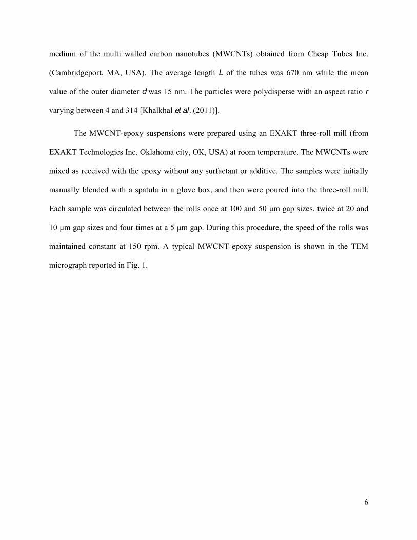
medium of the multi walled carbon nanotubes (MWCNTs) obtained from Cheap Tubes Inc.

(Cambridgeport, MA, USA). The average length L of the tubes was 670 nm while the mean

value of the outer diameter d was 15 nm. The particles were polydisperse with an aspect ratio r

varying between 4 and 314 [Khalkhal et al. (2011)].

The MWCNT-epoxy suspensions were prepared using an EXAKT three-roll mill (from

EXAKT Technologies Inc. Oklahoma city, OK, USA) at room temperature. The MWCNTs were

mixed as received with the epoxy without any surfactant or additive. The samples were initially

manually blended with a spatula in a glove box, and then were poured into the three-roll mill.

Each sample was circulated between the rolls once at 100 and 50 m gap sizes, twice at 20 and

10 m gap sizes and four times at a 5 m gap. During this procedure, the speed of the rolls was

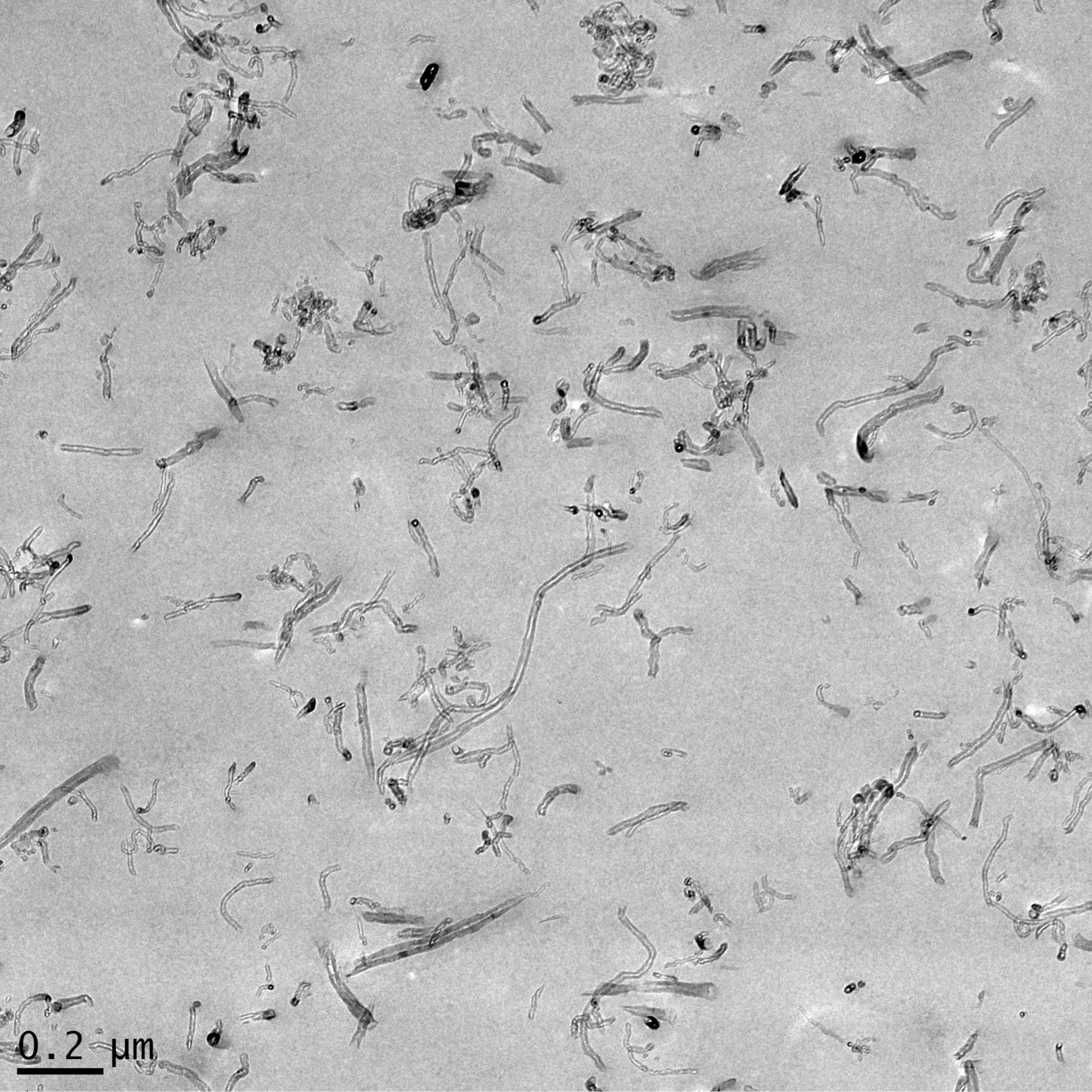
maintained constant at 150 rpm. A typical MWCNT-epoxy suspension is shown in the TEM

micrograph reported in Fig. 1.

7

Fig. 1 TEM micrograph of a cured epoxy-based suspension containing 3wt% MWCNTs.

Flow dichroism experiments were performed using a Couette cell (CC) and a parallel disk (PP)

setup. In the case of the Couette cell, the forward scattering data was collected in the flow-

gradient plane. The Couette cell had a height of 21 mm and inner and outer radii of 16.95 and

17.95 mm, respectively. The top and the bottom parts were made of quartz to send and collect

the laser light in the vorticity direction. Similarly, for the parallel disk setup the top and the

bottom disks were made of quartz. The disks had a diameter of 40 mm and the gap was varied

from 0.75 to 1.0 mm, depending on the concentration of MWCNTs such that the sample was not

opaque.

A home-built optical setup was employed to obtain dichroism data. The optical train is based on

field effect modulator as proposed by Frattini and Fuller (1984). A modulated polarization vector

8

of light is generated 632.8 nm, 10 mW He-Ne laser) through a

Glan-Thompson polarizer, P1-0° (Newport, RI, USA), which is parallel to the laser direction, a

photoelastic modulator, PEM-45° (Beaglehole Instruments, New Zealand) oriented at 45° with

respect to P1- 0° and a quarter wave plate, Q-0°, (Newport, RI, USA) oriented at 0° with respect

to P1-0°. The modulated light is then sent through the sample by a set of prisms. The harmonic

parts of the scattering data from the photodiode are sent to two lock-in amplifiers (Stanford

Research Systems model 530, Sunnyvale, CA, USA) and the intensity of the first harmonic (R1)

and the second harmonic (R2) data are recorded using a Labview program. The optical train is

arranged such that the scattering due to particle orientation in the flow direction corresponds to a

positive dichroism. The required flow field was applied using a MCR300 controlled stress

rheometer (Anton-Paar, Graz, Austria).

The flow dichroism is calculated from the extinction coefficient given by Fuller (1995):

2 2

1 1 22

1 2

1'' tanh2

R Rsign RJ A J A (1)

where 1J A and 2J A are Bessel functions of the first kind and A is the amplitude of the

photoelastic modulator adjusted to have 0 0J A . The extinction coefficient and flow

dichroism are related by the wavelength and the optical path length (sample thickness) via

[Fuller and Mikkelsen (1989)]:

''''

2n

l (2)

9

where l is the optical path length. Similarly, the orientation angle, , of the particles with

respect to the flow direction can be calculated using the data obtained by the two lock-in

amplifiers:

1 11

2 2

1 tan2

R J AR J A (3)

It should be noted that the orientation angle of the particles is only measurable in the Couette

flow cell because, in this case, the scattering data is collected in the vorticity direction. For

parallel disk geometry the measured orientation angle cannot be interpreted in a simple way and

this is out of scope for the current work.

Two tests were performed on the different samples and they are defined in this paper as shear

ramp and start-up tests. In shear ramp tests the samples were first allowed to rest for a

sufficiently long time in order to reach an isotropic initial orientation state before starting the

ramp in shear rates. In start-up tests, the samples were allowed to relax to an isotropic state

between each shear start-up at different imposed rates. A comparison of the results obtained at

each shear rate for the two tests will give us information about the influence of the initial

orientation state to the microstructure. Relaxation experiments were performed in the high Pe

regime so that all the particles were oriented and once the flow was stopped, particles underwent

relaxation to come back to an isotropic state due to Brownian motion. For all tests, the noise is

always lower than 9 % of the signal magnitude.

In order to obtain an initial isotropic orientation state, after loading the sample and before all the

tests, we applied a pre-shearing step at a rate of 10 s-1 for 100 s. Then, we let the samples relax

until all the dichroism vanished by observing its decay. Once the dichroism reached the lowest

value and was steady for 5 min (meaning the sample orientation state was isotropic) the lock-in

10

amplifiers were re-normalized to zero (the last value of dichroism was the baseline). The

MWCNT volume fraction, , varied between 75.6 10 and 31.39 10 from dilute to semi-dilute

regime. The limits between the two regimes are defined according to Doi and Edwards (1986)

and to Larson (1999) as:

2 3

2 3

1, 1 dilute;1, 1 semi-dilute.

cL d cLcL d cL

(4)

where c is the number of particle per unit volume. Thus, the dilute regime for the MWCNT

particles (average L = 670 nm and d = 15 nm) is 43.8 10 , while the upper limit of the semi-

dilute regime is 21.74 10 .

III. Dichroism in parallel disk and Couette flow geometries

The shear-induced dichroism, ''n , of the MWCNT suspensions in the disk (or parallel plate,

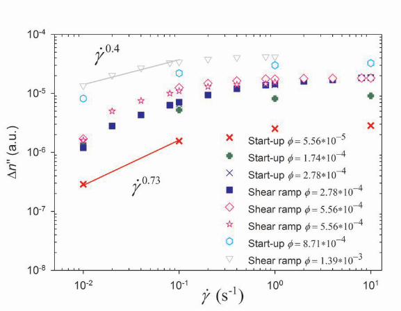
PP) flow geometry for different volume fractions is reported in Fig. 2.

11

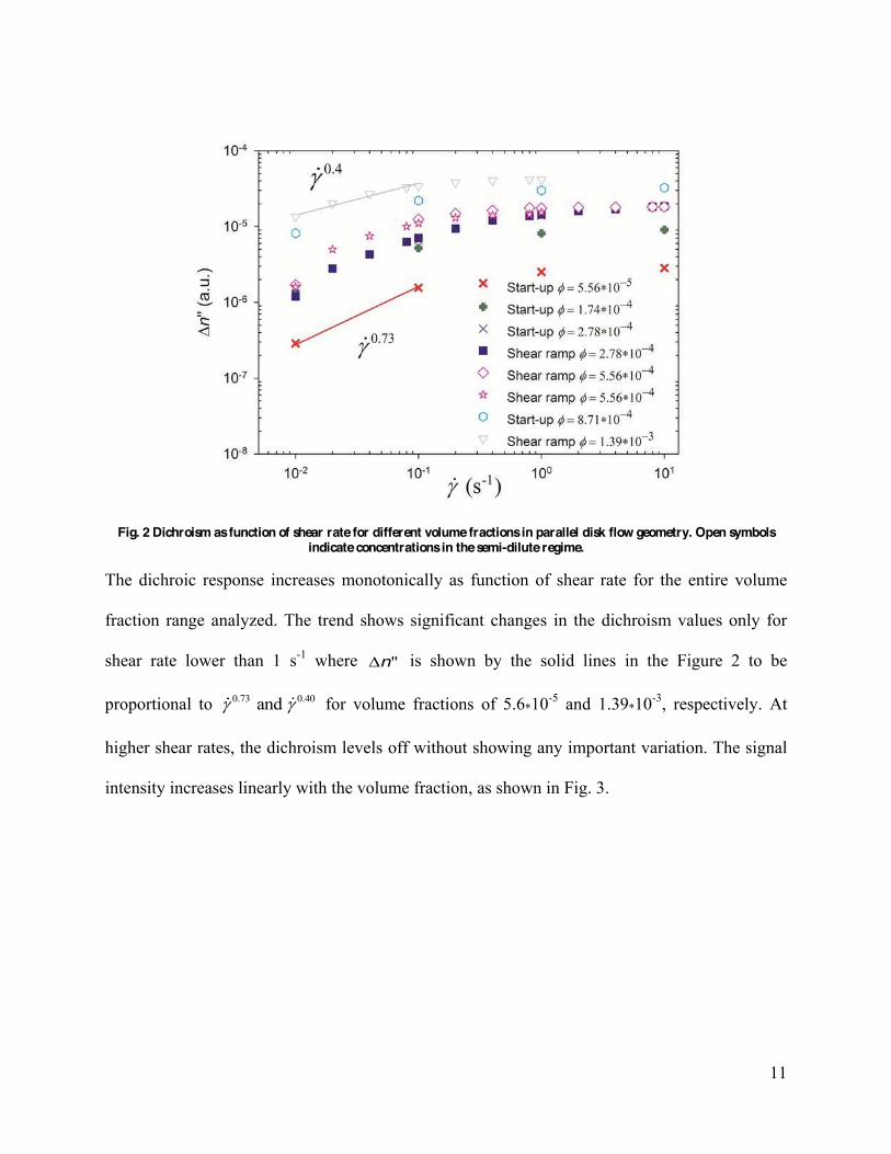
Fig. 2 Dichroism as function of shear rate for different volume fractions in parallel disk flow geometry. Open symbols indicate concentrations in the semi-dilute regime.

The dichroic response increases monotonically as function of shear rate for the entire volume

fraction range analyzed. The trend shows significant changes in the dichroism values only for

shear rate lower than 1 s-1 where ''n is shown by the solid lines in the Figure 2 to be

proportional to 0.73 0.40 and for volume fractions of 5.6*10-5 and 1.39*10-3, respectively. At

higher shear rates, the dichroism levels off without showing any important variation. The signal

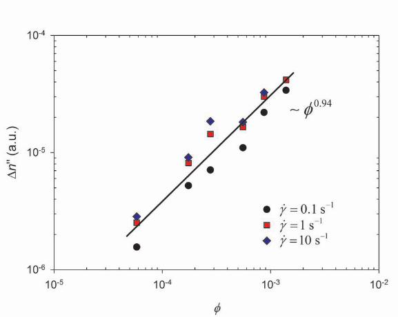
intensity increases linearly with the volume fraction, as shown in Fig. 3.

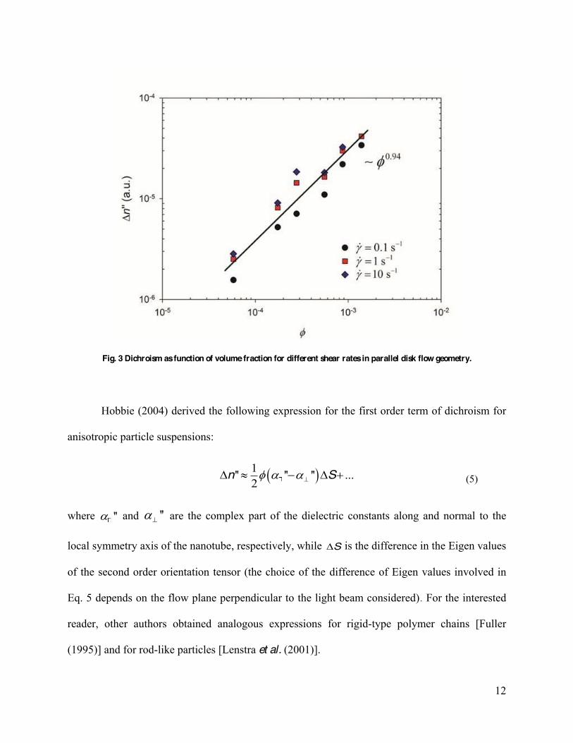
12

Fig. 3 Dichroism as function of volume fraction for different shear rates in parallel disk flow geometry.

Hobbie (2004) derived the following expression for the first order term of dichroism for

anisotropic particle suspensions:

1'' '' '' ...2

n S (5)

where '' and '' are the complex part of the dielectric constants along and normal to the

local symmetry axis of the nanotube, respectively, while S is the difference in the Eigen values

of the second order orientation tensor (the choice of the difference of Eigen values involved in

Eq. 5 depends on the flow plane perpendicular to the light beam considered). For the interested

reader, other authors obtained analogous expressions for rigid-type polymer chains [Fuller

(1995)] and for rod-like particles [Lenstra et al. (2001)].

13

Eq. 5 links the overall orientation of the system with the variation in dichroism. For a

perfectly isotropic orientation distribution, the optical response of the system will be about zero

(in a homogeneous system), while it will reach a maximum for a completely aligned state.

According to Eq. 5, the optical response in Fig. 2 is principally due to a more oriented system

with increasing flow intensity. At a shear rate larger than 1 s-1, the intensity does not change

anymore because of an already saturated orientation state. In the first decade of shear rate, the

slopes of the dichroism curves decrease with the volume fraction, going from 0.73 to 0.4 for

31.39 10 and 55.6 10 , respectively. In the dilute regime, the rods are free to rotate in

periodic orbits and, on average, align with the flow direction. As we move into the semi-dilute

regime, the interactions between the rods become more important since they scale 2O and

higher. The contacts between the rods cause a randomizing effect on the orientation distribution

of the fibers that is reflected in the shear rate dependency [Natale et al. (2014)].

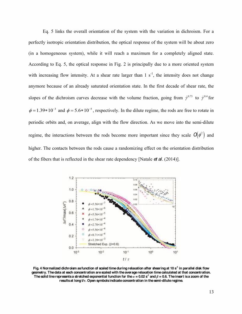
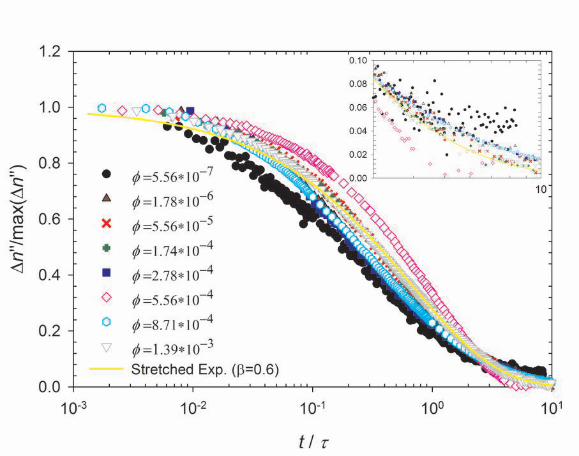
Fig. 4 Normalized dichroism as function of scaled time during relaxation after shearing at 10 s-1 in parallel disk flow geometry. The data at each concentration are scaled with the average relaxation time calculated at that concentration.

The solid line represents a stretched exponential function for the = 0.02 s-1 and = 0.6. The insert is a zoom of the results at long t/ . Open symbols indicate concentration in the semi-dilute regime.

14

The dichroism data relative to the relaxation step successive to shearing at 10 s-1 are reported in

Fig. 4 for different MWCNT concentrations. The curves are fitted with a stretched exponential

function, since a simple exponential function was not able to reproduce correctly the relaxation

behavior of these MWCNT suspensions:

'' expmax ''

n tn

(6)

The need for the stretched exponential is an evidence of multiple relaxation times in the system,

principally due to the polydispersed aspect ratio and flexibility of the MWCNTs. Conversely,

one can write the stretched exponential function as a sum of pure exponential decays weighted

by a particular probability distribution function of for a given value of [Johnston (2006)].

For each concentration, it is possible to calculate an average relaxation time from fitting the data

of Fig. 4:

0

1 1e t dt (7)

where is the gamma function. Once the relaxation time is known, the rotary diffusion

coefficient is evaluated as 16rD [Fuller (1995)]. The values obtained for , and rD are

reported in Fig. 5 and a stretched exponential function is reported in Fig. 4 for average values of

and .

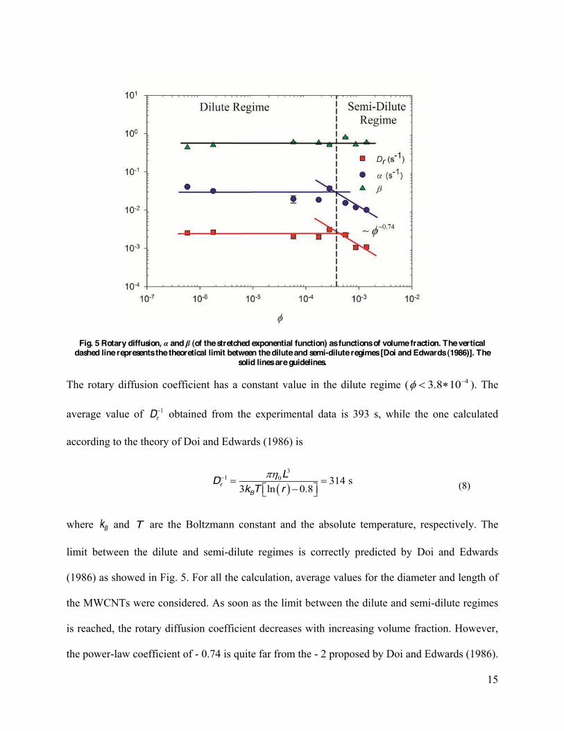
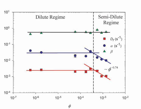
15

Fig. 5 Rotary diffusion, and (of the stretched exponential function) as functions of volume fraction. The vertical dashed line represents the theoretical limit between the dilute and semi-dilute regimes [Doi and Edwards (1986)]. The

solid lines are guidelines.

The rotary diffusion coefficient has a constant value in the dilute regime ( 43.8 10 ). The

average value of 1rD obtained from the experimental data is 393 s, while the one calculated

according to the theory of Doi and Edwards (1986) is

31 0 314 s

3 ln 0.8rB

LDk T r

(8)

where Bk and T are the Boltzmann constant and the absolute temperature, respectively. The

limit between the dilute and semi-dilute regimes is correctly predicted by Doi and Edwards

(1986) as showed in Fig. 5. For all the calculation, average values for the diameter and length of

the MWCNTs were considered. As soon as the limit between the dilute and semi-dilute regimes

is reached, the rotary diffusion coefficient decreases with increasing volume fraction. However,

the power-law coefficient of - 0.74 is quite far from the - 2 proposed by Doi and Edwards (1986).

16

This discrepancy could be attributed to the fact that only four points were considered to

determine this slope. More data in the semi-dilute regime would be needed to confirm this result.

Unfortunately, suspensions with higher MWCNT contents were too opaque to be probed

experimentally. In addition, a transition zone, where the volume fraction power-law index

changes gradually from 0 to - 2 between the two regimes, is expected. This transition zone is the

result of the polydispersity and flexibility of the particles that is not directly accounted for by Doi

and Edwards (1986). Since the analyzed semi-dilute volume fractions are close to the frontier

between the two regimes, they are possibly located in this transition zone, explaining the low

value of the power-law index (- 0.74) found experimentally.

The average value of the stretched exponential is around 0.6 and seems to be independent of

the volume fraction. As mentioned above, it is related to the polydispersity of the aspect ratio and

possible flexibility of the MWCNTs that result in a spectrum of relaxation times. On the other

hand, the value of has a similar behavior to the rotary diffusion and has units of s-1. Thus, it

describes the effect of excluded volume interactions between the rods [Bellini et al. (1989)].

The first order term of the refractive index tensor suggests (as shown in Eq. 5) a linear

dependency with the volume fraction. This is consistent with the scaling behavior firstly reported

by Fry et al. (2006).

17

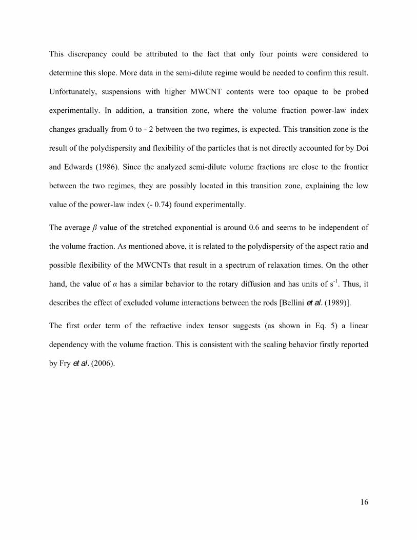
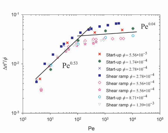
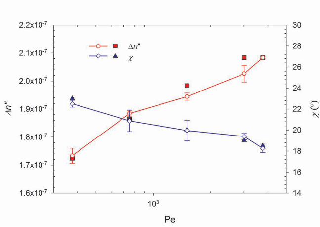
Fig. 6 Dichroism scaled with volume fraction as function of Peclet number in parallel disk flow geometry. Open symbols indicate concentrations in the semi-dilute regime.

In Fig. 6, the scaled dichroism is reported for the parallel disk data as a function of the rotational

Peclet number Pe rD . Data for the different concentrations are overlapping. The scaled

dichroism increases mainly for Pe lower than 102, where it is proportional to Pe1/2. This zone is

followed by a plateau where the dichroism changes slightly ( Pe0.04). This is in contrast with the

scaling behavior proposed by Fry et al. (2006). They found for their MWCNTs (with r four times

larger than the particles used in this work) at high Pe ( 4 910 Pe 10 ) that ''n was

proportional to 0.16Pe . This discrepancy might be because their suspensions were mainly in the

semi-dilute regime, implying that particle-particle interactions worked strongly against the

progressive alignment of the nanotubes.

18

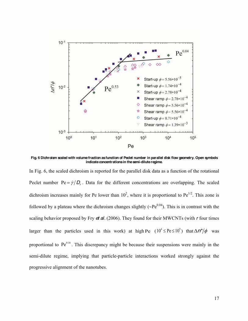
Fig. 7 Dichroism scaled with volume fraction and orientation angle as functions of Peclet number. The data were obtained in Couette cell (CC) and PP flow geometries. Open symbols refer to the orientation angle.

The same scaling is used in Fig. 7, where the values of dichroism and orientation angle obtained

in a Couette cell flow geometry for the dilute suspensions ( 43.8 10 ) are reported. In this

case, the light beam was perpendicular to the flow and velocity gradient plane, allowing for

direct evaluation of the angle between the principal axis of the particle and the flow direction.

It should be noted that for the lowest concentration ( 75.56 10 ) the dichroism signal was

quite low and it was not possible to obtain values for the orientation angle.

The dichroism shows a similar behavior to the results obtained in the disk or PP flow geometry.

For 2Pe 10 , ''n scales as 0.42Pe , hence with a slightly lower power-law index compared to

the one found for the PP geometry (0.53). For Pe < 1, it is expected that the first deviation from

an isotropic orientation state would be linear in the flow-gradient plane, while quadratic in the

19

flow-vorticity plane [Doi and Edwards (1986)]. Hence at low Pe, this could explain why a

stronger rate dependency is found in the PP geometry with respect to the one found in the

Couette flow cell. At high Pe, the slope of the dichroism curve tends to zero since change in

orientation is negligible (negligible slope for the orientation angle). The marginal effect of the

Brownian motion of these suspensions is clearly seen for 2Pe 10 where the orientation angle

changes quickly with increasing shear rate. Surprisingly, the orientation angle is far from zero

even at high Pe where it reaches the minimum value of 18 at 3Pe 4 10 . For concentrated

MWCNT suspensions, Pujari et al. (2011) found lower values of the orientation angle ( 5 )

from SAXS at -110 s . However, this shear rate for their combination of MWCNTs and matrix

corresponded to 6Pe 10 , three order of magnitude higher than the maximum Pe probed in our

work.

At high shear rates, the hydrodynamic force dominates the Brownian motion; hence, the

randomizing effect of the rotary diffusion cannot be the cause of the misalignment. In addition,

interactions between rods can also be excluded as a possible cause considering the very low

volume fraction (dilute regime) used in these experiments. The only other possible answer to

explain this peculiar behavior needs to be in the conformation of the rods. The TEM micrograph

in Fig. 1 obtained on a cured epoxy suspension shows that the equilibrium conformation of these

particles is far from being straight. This is mainly due to the presence of structural defects at the

MWCNT walls, which cause them to be bent [Hobbie (2004)].

The bending of the particles might be the cause of the behavior observed in Fig. 7 and its effect

is analyzed in the next section. For this purpose, a new model is developed based on the

hypothesis that the equilibrium conformations of MWCNTs are not straight but actually bent.

20

More specifically, we try to answer the following question: Is it possible that the misalignment

with respect to the flow direction at high Pe is due to the flexibility and bending of the rods, as

illustrated in Fig. 1?

IV. Model

Definitions and hypotheses

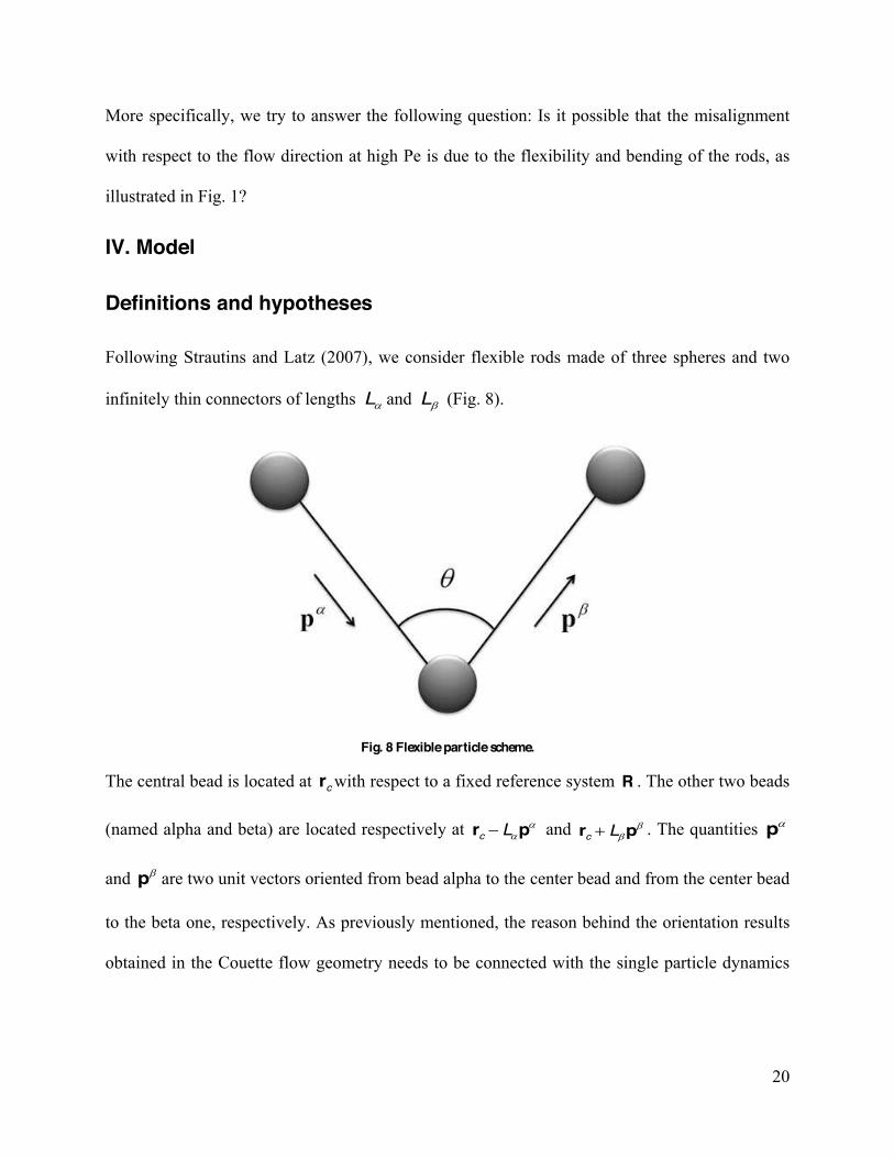
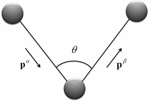
Following Strautins and Latz (2007), we consider flexible rods made of three spheres and two

infinitely thin connectors of lengths L and L (Fig. 8).

Fig. 8 Flexible particle scheme.

The central bead is located at cr with respect to a fixed reference system R . The other two beads

(named alpha and beta) are located respectively at c Lr p and c Lr p . The quantities p

and p are two unit vectors oriented from bead alpha to the center bead and from the center bead

to the beta one, respectively. As previously mentioned, the reason behind the orientation results

obtained in the Couette flow geometry needs to be connected with the single particle dynamics

21

and in particular, with particle conformation. The following hypotheses are stated for developing

the model to describe the behavior at high Pe number and in the dilute concentration regime:

1. All beads have the same mass and radius.

2. The particles are considered inertialess and the gravitational effect is negligible.

3. The suspended particles are assumed to be distributed uniformly, i.e., there is no

concentration gradient.

4. The bulk flow is assumed to be homogeneous and the velocity gradient

( v ) is constant over the particle length.

5. The particles have large aspect ratio and, hence, Brownian motion is neglected.

6. The matrix is considered incompressible and Newtonian with a viscosity 0 .

7. The particle flexibility is described according to a cosine harmonic potential and

the equilibrium positions of the particles are bent.

8. Particle-particle interactions are neglected.

Equations

Particle rotary velocity

In their work, Strautins and Latz (2007) proposed the following elastic potential to describe

flexibility:

1U k p p (9)

where k characterizes the resistance to bending. This potential allows only straight rods at

equilibrium or, in other words, it exhibits a minimum when the two rods are on a straight line.

This implies that in the absence of external forces the particles tend to simply assume a straight

22

rod configuration. As shown previously in Fig. 1, the MWCNTs are bent at equilibrium; hence,

to describe this behavior, a cosine harmonic potential [Bulacu et al. (2013)] is considered to be

acting on the particle to describe the bending resistance:

212

U k e p p (10)

The parameter k represents the stiffness of the particle while 1cos e is the equilibrium angle

between p and p . This potential is a restricted bending potential and allows us to describe

particles whose equilibrium position is far from a straight rod. An alternative approach was used

in Brownian dynamics simulations where the bending potential of Eq. 10 was coupled with a

priori chosen bent configuration [Cruz et al. (2012)].

To evaluate the rotary velocity of these flexible particles, it is necessary to write the evolution of

each connector. The hydrodynamic and bending forces act on each bead. From the force balance

derived in Appendix A, it is shown that the particle center of mass moves affinely with the flow

velocity. Hence, the spatial distribution of the rod center of mass remains homogenous under

flow. Considering the reference system on the central bead, the torque due to the hydrodynamic

force (proportional to the relative velocity between the fluid and the particle) on bead alpha is

written as:

H HL L L LT p F p (11)

where is the drag coefficient on a sphere.

In addition, the bending potential causes an intra-particle torque equal to:

23

B

U k eT p p p pp (12)

where is the unit tensor. The intensity of the bending torque is proportional to how far from

equilibrium the angle between the two rods is and its direction is perpendicular to the unit vector

p .

The sum of the two torques is equal to zero because of the inertialess assumption. After some

manipulations, the expression for the rotary velocity of the connector alpha is finally obtained:

2: k e

Lp (13)

Following the same procedure on the bead beta, the rotary velocity of p is calculated as:

2: k e

Lp (14)

In Eqs. 13 and 14, the orientation evolution is composed of two parts. The first two terms on the

right side of the equations correspond to the Jeffery equation for an ellipsoid of infinite aspect

ratio, while the last term is the coupling effect between the orientation of p and p due to the

introduction of the bending potential.

For the sake of completeness, the expression for the stress tensor is derived in Appendix B and

an approach to solve a modified Fokker-Planck equation for flexible rods is presented in

Appendix C. The approach leads to two new fourth-order non-symmetric tensors that require

closure approximations to solve the sets of equations. Instead of proposing questionable closure

approximations at this point, we use particle based simulations as described in the next section.

24

Particle based simulations

As discussed in Appendix C, we were not able to close the problem obtained writing the

orientation distribution function (ODF) moments evolution. In order to have first insights on the

predictions of the model, we proceed in this work with a particle-based simulation approach. It

consists in following the orientation evolution of a numerically significant number of particles to

accurately compute average properties. We are not required to solve the equation of the center of

mass velocity since we already know that the particles move homogenously with respect to the

fluid element at the same position. The numerical solution is obtained through a more simple set

of ordinary differential equations (ODEs). Thus, we firstly set a random initial orientation for N

particles. Then, we solve the ODEs (Eqs. 13 and 14) for each particle. Once we know the

orientation evolution of the N particles constituting the suspensions, we are able to calculate

2 d da p p p p , 2 d db p p p p and 2 d dc p p p p (Appendix C) by

numerically solving the integrals. For clarity, if we consider the tensor 2a , it is calculated as

follows:

( ) ( )

21

1 n nN

nd d

Na p p p p p p (15)

The value N is obtained numerically by finding the minimum number of particles above which

the values of the second order tensors become independent of N. It was found that N = 500 was a

sufficient number of particles and the following results are obtained with this value.

Since we assign randomly the initial position of each connector, we might start to shear a system

that it is not at equilibrium because some particles could be in a given conformation that is far

from their equilibrium. To avoid this problem, the initialization step is followed by a rest stage

25

where we solve Eqs. 13 and 14 for a shear rate equal to zero until steady state and only at this

point, we start shearing the system. The rest step allows the particles to relax until they reach

their equilibrium positions or, in other words, it allows dissipating the non-zero components of

the stress tensor due to the bending potential.

It is important to underline that since we are solving Eqs. 13 and 14, the particles are non-

Brownian. This implies that the predictions of the model are physically valid only at high Pe

numbers, which is fortunately the region of interest for this work.

V. Parametric analysis

The introduction of the bending potential brings into the model two adjustable parameters that

characterize the particles. The stiffness coefficient k has units of [N m] and it controls the

flexibility of the particles (higher k means lower flexibility). The equilibrium conformation e

defines the angle between p and p , when the bending potential reaches a minimum. In this

and following sections, we consider particles with connectors of the same length ( L L L )

and beads of the same diameter for simplicity purposes. From Eqs. 13 and 14, we can define the

following parameter:

2

1S

B

kkt L (16)

where Sk has units of s-1 and it represents the inverse of the characteristic bending time Bt . It is

chosen instead of parameter k avoiding defining particle length and diameter.

To better understand the predictions of the model, a first interesting aspect to analyze is the

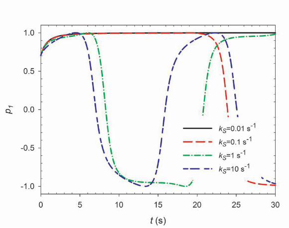
period of rotation of these flexible particles. For a clear representation, let us consider a single

particle in simple shear flow. To follow its evolution, it is straightforward to consider the

26

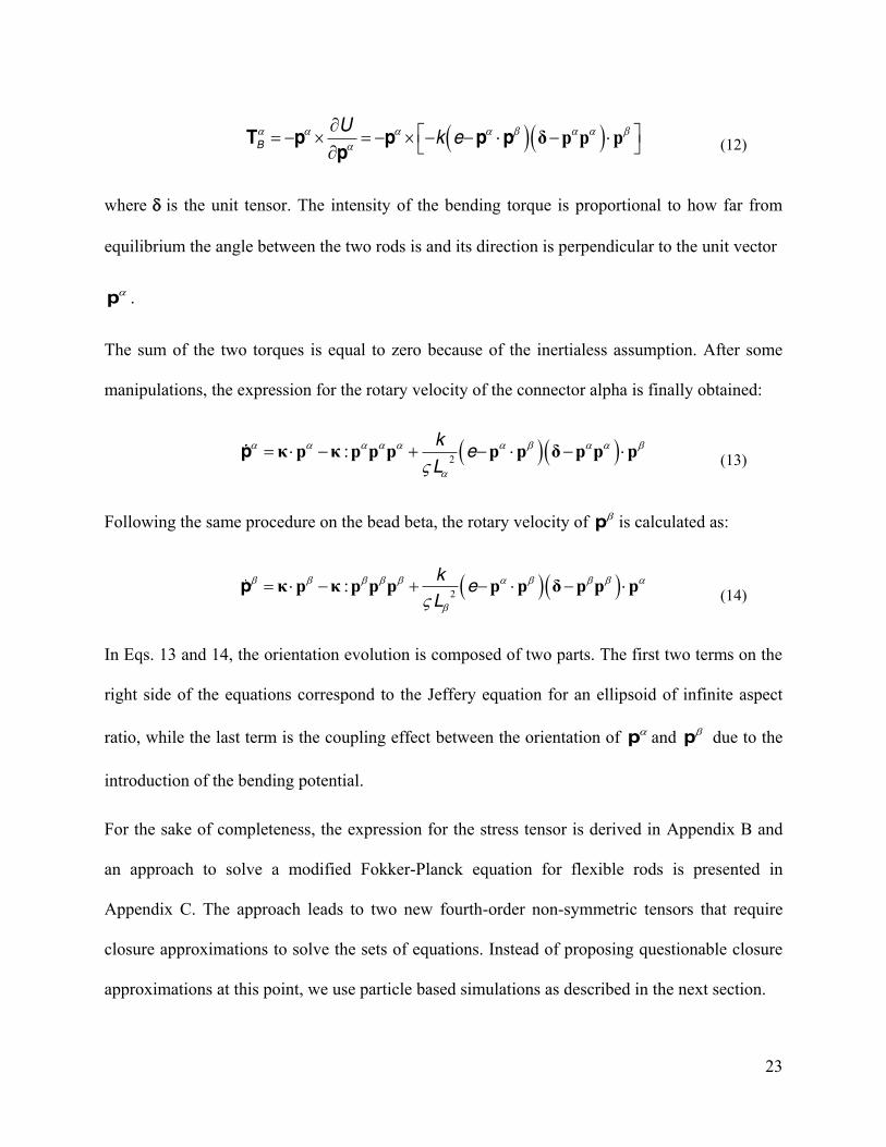
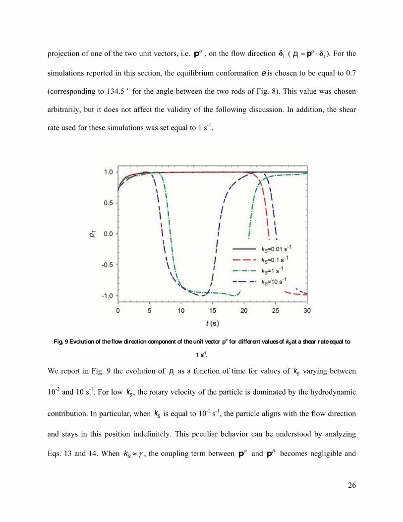
projection of one of the two unit vectors, i.e. p , on the flow direction 1 ( 1 1p p ). For the

simulations reported in this section, the equilibrium conformation e is chosen to be equal to 0.7

(corresponding to 134.5 o for the angle between the two rods of Fig. 8). This value was chosen

arbitrarily, but it does not affect the validity of the following discussion. In addition, the shear

rate used for these simulations was set equal to 1 s-1.

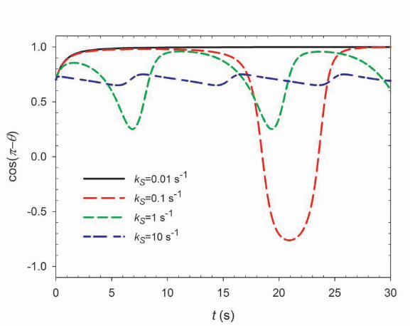
Fig. 9 Evolution of the flow direction component of the unit vector p for different values of kS at a shear rate equal to

1 s-1.

We report in Fig. 9 the evolution of 1p as a function of time for values of Sk varying between

10-2 and 10 s-1. For low Sk , the rotary velocity of the particle is dominated by the hydrodynamic

contribution. In particular, when Sk is equal to 10-2 s-1, the particle aligns with the flow direction

and stays in this position indefinitely. This peculiar behavior can be understood by analyzing

Eqs. 13 and 14. When Sk , the coupling term between p and p becomes negligible and

27

the particle behaves as a rod of infinite aspect ratio, accordingly to the Jeffery equation. With

increasing values of Sk , the particle becomes more and more rigid and it rotates in the gradient-

flow plane. The period of rotation becomes shorter as Sk increases since the torque due to the

bending potential is more intense. Each connector pulls and pushes the other one during the

rotation, keeping the angle between p and p around the equilibrium position.

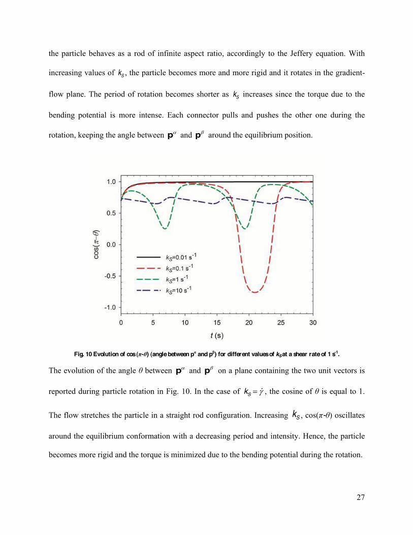
Fig. 10 Evolution of cos ( - ) (angle between p and p ) for different values of kS at a shear rate of 1 s-1.

The evolution of the angle between p and p on a plane containing the two unit vectors is

reported during particle rotation in Fig. 10. In the case of Sk , the cosine of is equal to 1.

The flow stretches the particle in a straight rod configuration. Increasing Sk , cos( - ) oscillates

around the equilibrium conformation with a decreasing period and intensity. Hence, the particle

becomes more rigid and the torque is minimized due to the bending potential during the rotation.

28

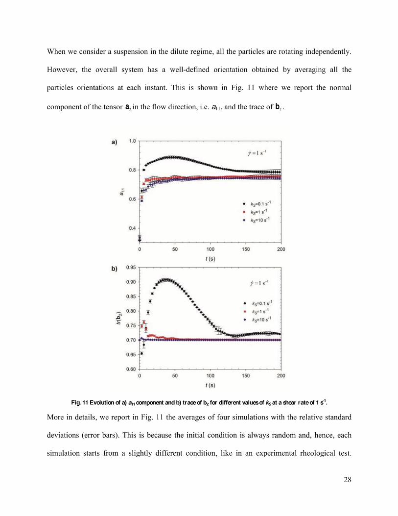
When we consider a suspension in the dilute regime, all the particles are rotating independently.

However, the overall system has a well-defined orientation obtained by averaging all the

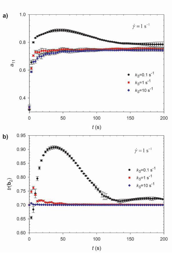
particles orientations at each instant. This is shown in Fig. 11 where we report the normal

component of the tensor 2a in the flow direction, i.e. a11, and the trace of 2b .

Fig. 11 Evolution of a) a11 component and b) trace of b2 for different values of kS at a shear rate of 1 s-1.

More in details, we report in Fig. 11 the averages of four simulations with the relative standard

deviations (error bars). This is because the initial condition is always random and, hence, each

simulation starts from a slightly different condition, like in an experimental rheological test.

29

Since we start from an isotropic state, the evolutions of the 2c components are similar to the ones

of 2a , and for the sake of brevity are not reported here. The a11 component (Fig. 11a) presents a

significant overshoot for < Sk while it increases monotonically for Sk to reach rapidly

steady state. Under steady state, the more flexible particles ( -10.1 sSk ) get more aligned in the

flow direction. Analyzing the trace of 2b in Fig. 11b, which represents the average cosine of the

angle between the connectors p and p [Ortman et al. (2012)], it becomes clear that the

overshoot in a11 for < Sk is due to the stretching effect of the shear flow that opens up the

particles in a - configuration, and aligns them in the flow direction. In this case, the

trace of 2b presents a large overshoot and then levels off towards the equilibrium value. As Sk

increases, the intensity of the overshoot decreases until almost disappearing. This behavior is due

to the fact that the average conformation angle does not vary significantly with respect to the

chosen equilibrium position.

On the other hand, parameter e controls the equilibrium angle between the two connectors. It

does not influence the time evolution of the particles, but it determines variations in the degree of

orientation under steady state (not shown here). The straighter the particles are, the more they

tend to align in the flow direction as they slow down their rotation when in the flow direction.

Again, these considerations are valid only in the dilute regime.

Concluding this section, a distinction needs to be made between quenched and strain-induced

bending. In our simple model, the parameter e controls the particle equilibrium conformation;

hence, the particle is in this

conformation, no torque due to the bending potential acts on the particle arms. In the presence of

flow, the hydrodynamic torques can displace the arms from the equilibrium position, causing

30

stretching or more pronounced bending. The competition between the hydrodynamic and

bending torques, which is controlled by the ratio Sk , will determine the evolution of the

conformation of the particle during flow. In this scenario, we refer to strain-induced bending.

Finally, no thermal bending is present in the model since the effect of Brownian motion is

neglected here.

VI. Predictions at high Pe

We are interested now in explaining the high values of the orientation angle shown in Fig. 7. To

quantify the flexibility of the rods, the effective stiffness is calculated as 464effY sS E r

[Switzer III and Klingenberg (2003)] where YE is the Young modulus of the MWCNTs and is

considered to be 40 GPa according to Hobbie and Fry (2007). We underline that a precise value

for the Young modulus might be highly depending of the specific sample, but the following

analysis is sensitive only to order of magnitude changes. Using an average aspect ratio r of 45,

the value of effS can be estimated to be in the range of 3.8 to 38.5 for our MWCNTs. Hence, we

can consider that on average these particles are moderately stiff in the range of shear rates

analyzed.

To represent this complex system with our mathematical description, we chose a value of 1 s-1

for the parameter Sk that is of the same order of the shear rates analyzed 0.1,1Sk ,

guaranteeing that the particles are sufficiently stiff in comparison with the flow intensity.

Parameter e was obtained by fitting the steady-state values of the orientation angle at each shear

rate. The effective stiffness effS presents a strong dependency on the aspect ratio. Our MWCNTs

are polydispersed in length and diameter and, nevertheless, they act overall as moderately stiff, a

spectrum of behaviors ranging from rigid to completely flexible is present. Therefore, the

31

equilibrium angle is assumed to be a function of the shear rate in order to keep into consideration

this large range of behaviors.

Following Fuller (1995) who expressed dichroism and orientation angle for rigid rod suspensions

as functions of the orientation tensor, the expression is here modified to account for the particles

made of two connectors as follows:

0.5 0.52 2 2 2 2 211 22 12 11 22 12'' 4 4

2n M a a a c c c

12 12

11 22 11 22

1 2 2tan(2 )2

a ca a c c

(17)

where M is a proportionality constant associated with the intrinsic optical anisotropy of the

system and is determined by comparing the predictions with the experimental values. Since our

particles are made of two arms, ''n and are obtained as algebraic means of the alpha and

beta connector contributions.

32

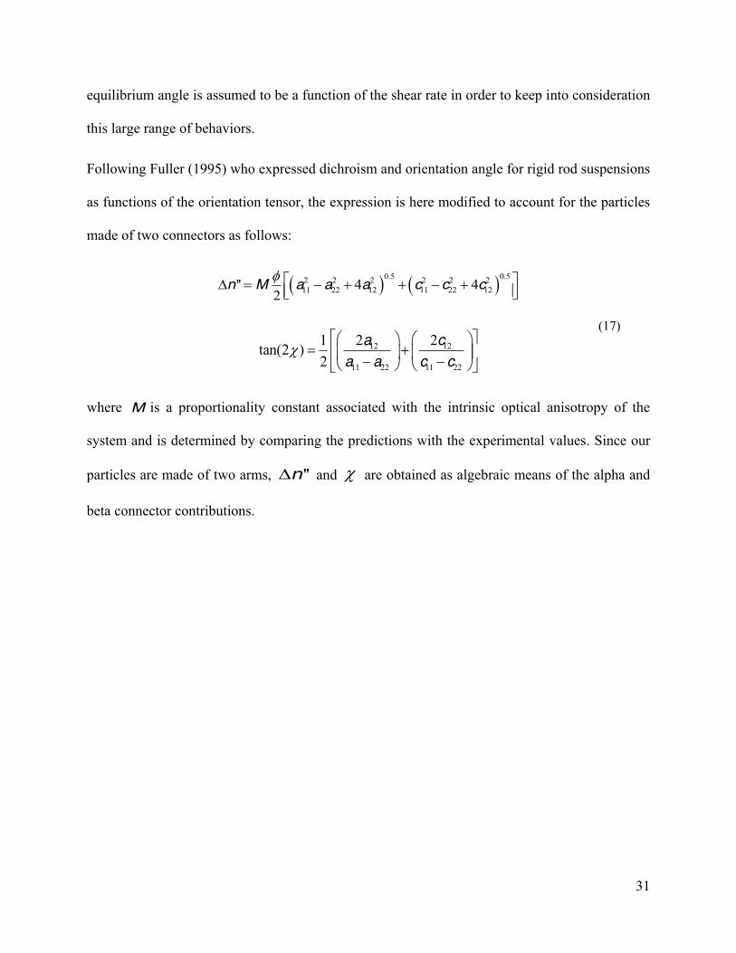
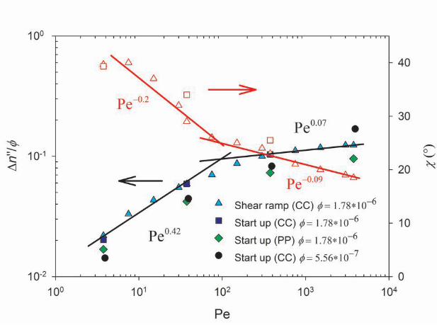
Fig. 12 Comparison between experimental (filled) and predicted (unfilled) values of dichroism and orientation angle obtained in the Couette flow geometry.

Fig.12 compares the experimental and predicted values for dichroism and orientation angle for

2Pe > 10 obtained in the Couette flow geometry using Sk equal to 1 s-1 and e as a fitting

parameter. As previously discussed, the predictions of the model obtained for particle-based

simulations without the addition of stochastic terms to represent Brownian motion are physically

valid only in this high Pe regime. As seen in Fig. 12, the model is able to correctly predict the

rheo-optical behavior of the dilute epoxy-MWCNT system, confirming that the equilibrium

conformation of these MWCNTs is not straight but bent. The values of e obtained by fitting the

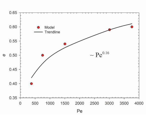
orientation angle are presented in Fig. 13.

33

Fig. 13 Fitted values for the equilibrium position e as a function of Pe. The trendline represents the regression of the data with a power-law expression.

As the intensity of the flow increases, the particles get more and more straight. The equilibrium

position scales as 0.16Pe showing a stronger dependency than the one found experimentally for

the orientation angle 0.09Pe (Fig. 7). The value of the exponent (0.16) in Fig. 13 is obtained by

a regression of the data with a power-law expression. Conversely, the flow efficiency in aligning

the particles is here lowered due to the fact that the particles can bend to disperse the flow

energy.

From the ratio between the predicted and experimental dichroism, the value of M , which is

related to the intrinsic anisotropy and polarizability of MWCNTs in epoxy, is found to be

172 10 mL, about 5 order of magnitude larger than the values reported by Chow et al. (1985a)

for collagen in a glycerin-water mixture.

34

Concluding, the high values of the orientation angle with respect to the flow direction are found,

with the help of a simple model, to be caused by particle bending and flexibility. Indeed, particle

stretching induces a more oriented system, as confirmed by the good agreement between the

model predictions and experimental data for ''n and . This is a consequence of the

interplay between particle conformations and hydrodynamic torques. The hydrodynamic torque

for these slender bodies exhibits a minimum in the case of straight particles perfectly oriented in

the flow direction. Hence, the system tries to reach that state, but is limited by the imposed

bending potential that traps the system in a different conformation which depends on the

imposed shear rate.

VII. Concluding remarks

Dichroism evolution of non-Brownian epoxy-based MWCNT suspensions can be divided into

two regimes. For 2Pe < 10 , MWCNTs are partially aligned in the flow direction due to

hydrodynamic forces, while for higher Pe , the already saturated orientation state of the system

changes slightly. Doi and Edwards (1986) theory was found to predict correctly the limit

between the dilute and semi-dilute regimes. However, their theory predicts that dichroism scales

with 0.25Pe in the case of semi-dilute suspensions at modest Peclet numbers and this is not in

agreement with our experimental findings ( 0.53Pe and 0.42Pe in the case of PP and CC geometry,

respectively).

Unlike other rod-like particles, for example collagen, MWCNTs show high values of the

orientation angle (~ 18°) in the high Pe region investigated in this work. Our simple model

confirmed that this behavior is mainly due to a non-straight equilibrium conformation of the

particles. In the model, orientation dynamic of flexible slender bodies is controlled by

35

hydrodynamic and bending torques. The bending torque is caused by a cosine harmonic potential

assumed to be acting between the two connectors of a particle. This potential is also responsible

for the bent configuration at equilibrium. We found that the interplay between hydrodynamic and

bending contributions causes an orientation evolution completely different with respect to the

one for slender rigid rods, which completely align in the flow direction. Particles keep tumbling

even if their aspect ratio is infinite because of the bending torque.

In addition, we found that the high values of the orientation angle are well predicted by the

model and the slight change of dichroism intensity in this saturated orientation level is mainly

due to rod stretching. On average, particles become straighter with increasing shear rate.

Particle-based simulations were used here in order to confront experimental data with model

predictions. However, the absence of stochastic terms in the simulations limits the predictions to

the regime where the Brownian contribution to the orientation evolution is negligible. Future

work will focus on the introduction of a stochastic term or in the solution of the modified

Fokker-Planck equation for flexible rods (Eq. C1 of Appendix C). Furthermore, it would be most

useful to find a solution for the closure problem in solving fourth order orientation tensors, which

are non-symmetric tensors. Finally, another interesting aspect to be analyzed is the direct

introduction of polydispersity, not only in the connector lengths, but also in the equilibrium

conformation. This will introduce a continuous spectrum of relaxation times that could explain

the mild elasticity (low values of ) found for dilute MWCNT suspensions in small amplitude

oscillatory flow [Ma et al. (2008)] and, in addition, the fast change in anisotropy during rest after

shearing brought to light by Pujari et al. (2011).

Acknowledgements

36

This work was funded by NSERC (Natural Science and Engineering Research Council of

Canada). The authors are profoundly thankful to Dr. Jan Vermant and Dr. Paula Moldenaers for

providing access to their rheo-optical setup at KU Leuven and for insightful discussions.

Appendix A: Force Balance

Since 0U r and the beads are inertialess and non-Brownian, the only force acting on the

beads is the hydrodynamic force:

3 3 0c c L L L L (A1)

The position of the center of mass cmr considering the three beads having the same mass is

33

ccm

L Lr p pr (A2)

and its velocity cmr is

33

ccm

L Lr p pr (A3)

Substituting Eqs. A2 and A3 into Eq. A1, we obtain:

0cm cm

cm cmr (A4)

The center of mass has an affine motion with the fluid velocity, hence no spatial gradients are

present in the system. This respects the third hypothesis.

Appendix B: Derivation of the stress tensor

37

In this section, we report for completeness the derivation of the stress tensor for our flexible

particle model. The contribution to the stress tensor due to the presence of particles in the matrix

is defined according to the Kramers-Kirkwood expression [Bird et al. (1987)] as follows:

1 1 1H Bp i i i i i i

i i iV V V (B1)

where HiF , B

iF and ir are the hydrodynamic force, the bending force and the position of the bead

i. Let us start analyzing the hydrodynamic contribution to the stress tensor:

3Hi i c c c

i

c c

c c

L L L L

L L L

L L L

r F r

p

p

(B2)

The first bracket on the right is equal to zero since the particle center of the mass moves with the

fluid element. We can write c c as a function of the position of the center of mass from

Eq. A1 obtaining:

3 3c c cm cm

L L L L (B3)

The first term on the right-end side of Eq. B3 is zero for affine motion. Substituting Eq. B3 in

Eq. B2, we obtain:

23 3

23 3

Hi i

i

L LL L L

L LL L L

r F p

p

(B4)

and assuming affine rotation, we finally get:

38

2 1: :3 3

2 1: :3 3

Hi i

iL L L

L L L

r F p

p (B5)

Hence, the contribution to the stress due to the hydrodynamic force is:

2

2

1

2 1: :3 32 1: :3 3

HH i i

iV

n L d d L L d d

n L d d L L d d

(B6)

Now, let us calculate the contribution to the stress tensor due to the bending potential:

Bi i c

i

k ke eL L

kL eL

kL eL

r F r p p

p p p

p p p

(B7)

The first term on the right-end side of Eq. B7 is zero since 0c cdr r . Simplifying, we get:

Bi i

ik e

k e

r F p p p

p p p (B8)

Hence, the contribution to the stress tensor due to the bending potential is:

39

1 BB i i

iV

nk e d d

nk e d d

p p p p p p p p p p

p p p p p p p p p p

(B9)

After some rearrangements, the bending contribution to the stress tensor is given by:

2 2

2

B nke

nk e e d d

nk d d

p p p p p p p p p p p p

p p p p p p p p

(B10)

The total stress tensor can now be calculated by adding the matrix contribution to the

hydrodynamic and bending contributions obtained in Eqs. B6 and B10.

Appendix C: Second order orientation tensors

The multitude of particles constituting a suspension requires a statistical description of the

problem. Therefore, an orientation distribution function, , ,tp p , is introduced (valid

for a spatially homogeneous system). It describes the probability of finding particles whose

connectors have a certain orientation in space at a given instant. The orientation distribution

function (ODF) can be regarded as a convected variable in the R5 space described by all the

possible configuration of p and p . Hence, the dynamics of a system under the hypotheses

previously stated is depicted by the following modified Fokker-Planck equation for flexible rods:

2 2

2 2rD DDt

p pp p p p

(C1)

40

In Eq. C1, a diffusion term, representing the effect of the rotary Brownian motion, is added in

order to have a description valid for all Pe numbers and aspect ratios. In this section, hypothesis

5 is removed to obtain equations with a more general form. The numerical solution of this partial

differential equation would require an enormous computational effort since a nonstandard R4

space and time variable are required to be meshed. Consequently, a different strategy needs to be

adopted.

One possibility is the definition of appropriate orientation tensors to describe the overall

orientation evolution of the system [Advani and Tucker (1987)]. Of course, the information

contained in a finite number of ODF moments is inferior to the knowledge of the full .

However, it is often sufficient to calculate average quantities of interest, i.e. stress tensor

components, dichroism and average orientation angle. For our system, the time evolution of three

second order orientation tensors is needed to completely describe the change in the

microstructure. This comes out naturally from the mathematical development below. Following

Ortman et al. (2012), an obvious choice of a second order tensor is the one related to the

orientation of the connectors from the bead alpha to the central one: 2 d da p p p p .

The time evolution of 2a is calculated as follows:

2D d d d d

Dta p p p p p p p p (C2)

Substituting Eq. 13 in the last equation and after some lengthy calculations, we obtain:

41

22 2 2 2 4 2

2 22

2

2

1 1 ( 2 ) 2 32 2

2

2

rD DDt

k e d dLk d d d dL

a a a a a a

b b p p p p p p

p p p p p p p p p p p p p p

(C3)

where 2 d db p p p p and 4 d da p p p p p p . and are the deformation rate

and the vorticity tensor. The presence of the fourth order orientation tensor 4a implies the need

of a closure approximation to solve the problem. Further approximations are also necessary to

compute the last three integrals on the right side of Eq. C3. It is important to underline that the

second order tensor 2b is not symmetric. This is due to the fact that we removed the hypothesis

of semi-flexibility (p p ) that guaranteed the symmetry of the mixed tensor in the work of

Ortman et al. (2012).

It can be easily seen that to compute the rate of change of 2a , Eq. C3 requires knowledge of the

evolution for the second order tensor 2b . Following the same procedure applied for 2a and

making use of Eqs. 13 and 14, the rate of change for 2b is written as

22 2 2 2 2 2

2 22 2 2 2

2 2 2 2

1 1 22 2

12

1 1

1 1

rD DDt

d d d d

ke d dL L L L

k d dL L L L

b

p p p p p p p p p p p p

a c p p p p p p

p p p pp p p p2

d dp p p p p p

(C4)

42

The tensor 2b contains information regarding the average spatial conformation of the particles. In

particular, the trace of 2b is equal to d dp p p p and it represents the average cosine of

the angle between the connectors p and p [Ortman et al. (2012)]. As a consequence, the trace

of 2b is no longer unitary as for the other non-mixed second order tensors presented here. It

varies between 0 and 1 corresponding to a system of bent or straight particles, respectively.

The time evolution of the mixed tensor 2b introduces the need of a time evolution for a third

orientation tensor 2 d dc p p p p . It represents the average orientation of the connectors

p . Proceeding as previously, its time evolution can be obtained as:

22 2 2 2 4 2

2 22

2

2

1 1 ( 2 ) 2 32 2

2

2

rD DDt

k e d dLk d d d dL

c c c c c c

b b p p p p p p

p p p p p p p p p p p p p p

(C5)

where 4 d dc p p p p p p . These three orientation tensors contain sufficient information

to calculate average quantities of interest.

Ortman et al. (2012) proposed a simple approximation for the integrals containing the dot

product between p and p . As an example, let us consider the integral

d dp p p p p p . It can be written as follows:

2 2d d d d d d trp p p p p p p p p p p p p p b a (C6)

43

One could similarly approximate the other integrals that contains the dot product between p

and p . Unfortunately, we are still not able to close the problem due to the presence of two new

fourth order orientation tensors in Eq. C4: d dp p p p p p and d dp p p p p p .

These last two tensors are non-symmetric tensors, while all the closure approximations reported

in the literature have been developed in order to preserve the symmetry of fourth order

orientation tensors like 4a and 4c [Advani and Tucker (1987), Cintra and Tucker (1995)]. Hence,

their proposed closure approximations would not work in this particular case. For the first time,

the closure approximation problem is here extended to anti-symmetric tensors. To our

knowledge, no solution is available in the literature and thus, we open up this question to the

scientific community.

REFERENCES

Abbasi S., P. Carreau, A. Derdou48,

943-959 (2009).

Abdel- -multi -Newtonian Fluid Mechanics 128, 2-6 (2005).

31, 751-784 (1987).

-exponential relaxation of 10,

499 (1989).

Bird R. B., C. F. Curtiss, R. C. Armstrong and O. Hassager, Dynamics of polymeric liquids. Volume 2, Kinetic theory (Wiley, New York, 1987).

Bulacu M., N. Goga, W. Zhao, G. Rossi, L. Monticelli, X. Periole, D. P. Tieleman and S. J. -Grained Molecular Dynamics

Simulation 9, 3282-3292 (2013).

chains subject to transient shear flow. 2. Two-color flow birefringence measurements on collagen p 18, 793-804 (1985a).

44

18, 805-810 (1985b).

Cintra J. J. S. and C. L. Tucke -induced fiber 39, 1095-1122 (1995).

-strain step response in linear regime of dilute suspensions of naturally bent carboScience 125, 4347-4357 (2012).

-like macromolecules in concentrated solution. Part 74, 560-570 (1978).

37, 9048-9055 (2004).

Fan Z. and Rheology 51, 585-604 (2007).

Reinf. Plast. Compos. 3, 99 (1984).

-

Science 100, 506-518 (1984).

Fry D., B. Langhorst, H. Wang, M. L. Becker, B. J. Bauer, E. A. Grulke and E. K. Hobbie, -

124, 054703 (2006).

Fuller G. G., Optical rheometry of complex fluids (Oxford University Press, 1995).

Fuller G. G. and K. J. Mik-present) 33, 761-769 (1989).

121, 1029-1037 (2004).

Hobbie E. K. Journal of Chemical Physics 126, 124907-7 (2007).

conductivity and rheology in poly(ethylene terephthalate) through the networks of multi-47, 480-488 (2006).

73, 125422 (2006).

Johnston D. 74, 184430 (2006).

45

Keshtkar M., M.-and microstructural evolution of semi-Journal of Rheology (1978-present) 54, 197-222 (2010).

-up at rest in MWCNT -Newtonian Fluid Mechanics 171 172, 56-66 (2012).

and the evolution of the structure of multiwalled carbon nanotube suspensions in an 55, 153-175 (2011).

Lar

-induced displacement of isotropic-nematic 114, 10151-10162 (2001).

Ma W. K. A., F. 52, 1311-1330 (2008).

viscosity of rodPolymer Letters Edition 21, 83-86 (1983).

nanotube suspensions with rod AIChE Journal 60, 1476-1487 (2014).

85, 1190-1197 (1986).

Ortman K., D. Baird, P. Wapperom and A. Whsliding plate rheometer to determine material parameters for the purpose of predicting

-present) 56, 955-981 (2012).

Pujari S., S. Rahatekar, J. W. Gilman -induced anisotropy of concentrated multiwalled carbon nanotube suspensions using x-ray

-present) 55, 1033-1058 (2011).

Pujari S., S. S. Rahatekar, J. W. Gilman, K. K. Koziol, A. H. Windle and W. R. Burghardt,

The Journal of Chemical Physics 130, - (2009).

Rahatekar S. S., K. K. K. Koziol, S. A. Butler, J. A. Elliott, M. S. P. Shaffer, M. R. Mackley and

-present) 50, 599-610 (2006).

s of Semiflexible Fibers in Polymeric 44, 521-535 (2005).

fiber interactions on rheology and flow behavior of suspensions of semi-flRheologica Acta 47, 701-717 (2008).

-Rheologica Acta 46, 1057-1064 (2007).

46

sheared flexible fiber suspensions via fiber- 47, 759-778 (2003).

-walled carbon nanotube/poly(butylene mer Physics 45,

2239-2251 (2007).