RG flows from Spin(7), CY 4-fold and HK manifolds to AdS, Penrose limits and pp waves

arX

iv:h

ep-t

h/02

0312

4v3

12

Jul 2

002

hep-th/0203124CTP-MIT-3251

DAMTP-2002-33

RG flows from Spin(7), CY 4-fold and HK manifolds toAdS, Penrose limits and pp waves

Umut Gursoy1,a, Carlos Nunez2, Martin Schvellinger1,b

1Center for Theoretical Physics,

Laboratory for Nuclear Science and Department of Physics,

Massachusetts Institute of Technology,

Cambridge, Massachusetts 02139, USAa E-mail: [email protected]

b E-mail: [email protected]

2Department of Applied Mathematics and Theoretical Physics,

Centre for Mathematical Sciences, University of Cambridge,

Wilberforce Road, Cambridge CB3 0WA, U.K.

E-mail: [email protected]

Abstract

We obtain explicit realizations of holographic renormalization group (RG) flows from M-

theory, from E2,1 × Spin(7) at UV to AdS4 × S7 (squashed S7) at IR, from E2,1 × CY 4 at

UV to AdS4×Q1,1,1 at IR, and from E2,1×HK (hyperKahler) at UV to AdS4×N0,1,0 at IR.

The dual type IIA string theory configurations correspond to D2-D6 brane systems where

D6-branes wrap supersymmetric four-cycles. We also study the Penrose limits and obtain

the pp-wave backgrounds for the above configurations. Besides, we study some examples of

non-supersymmetric and supersymmetric flows in five-dimensional gauge theories.

1 Introduction

Since M-theory compactifications on manifolds of special holonomy preserve a fraction of the

original supercharges in flat eleven-dimensional spacetime, it has become a fruitful arena to

explore the dynamical aspects of minimally supersymmetric gauge theories. Indeed, study of

special holonomy manifolds developing an isolated classical singularity has recently shed light

on several important questions regarding restoration of global symmetries, phase transitions

between different classical spacetimes [1, 2, 3, 4, 5, 6, 7, 8, 9, 10, 11, 12, 13, 14, 15, 16, 17,

18, 19, 20, 21, 22, 23, 24, 25, 26, 27, 28], relations between anomalies in M-theory, string

theory and gauge theories [3], among other relevant aspects (see for instance [6] to [26]).

The dynamics of N = 1 SYM theory in four and three dimensions has been exhaustively

investigated by Atiyah and Witten [2] and Gukov and Sparks [3], respectively.

Particularly, it is possible to study certain properties of these backgrounds through their

dual D6 brane configurations in type IIA string theory. Any configuration of type IIA string

theory with no bosonic content except than the metric, Ramond-Ramond one-form and

dilaton lifts to an eleven-dimensional supergravity configuration without flux. This is a pure

gravitational configuration. For instance, let us consider a collection of N6 parallel D6-branes

in type IIA string theory [29]. In eleven dimensions the metric is described by the product of

a seven-dimensional Minkowski spacetime and an Euclidean multi-centered Taub-NUT space

[30]. Moreover, a configuration of D6-branes in flat space can be represented in M-theory by

a four-dimensional manifold with SU(2) holonomy [7]. Furthermore, one can consider D6-

branes wrapping supersymmetric cycles in spaces with special holonomy and, as described

in [7], there are two different possibilities that can be exemplified as follows. One can have

D6-branes wrapping a supersymmetric four-cycle, S4, in a G2 holonomy manifold. Thus,

D6-branes completely fill the space transverse to type IIA string theory compactification

manifold, and therefore the field theory is on the transverse Minkowski three-dimensional

spacetime, while the local M-theory description involves a Spin(7) holonomy manifold. As

another example, one can consider D6-branes wrapping a different four-cycle, S2 × S2, in

a CY3 fold. Then, the three-dimensional field theory is codimension one in the transverse

Minkowski space to the type IIA compactification manifold. In this case, the local M-theory

description is given by a CY4 fold. The corresponding pure eleven-dimensional geometric

configurations were obtained long time ago in [31] and [32]. Recently, a supergravity solution

was obtained when D6-branes are wrapped on S4 in seven-dimensional manifolds of G2

holonomy [33]. This solution preserves two supercharges and thus it represents a supergravity

dual of a three-dimensional N = 1 SYM theory. Lifted to eleven dimensions this solution

describes M-theory on the background of a Spin(7) holonomy manifold. A detailed analysis

of the dual field theory has been done in [3]. In addition, supergravity duals of D6-branes

wrapping Kahler four-cycles inside a CY3 fold have been obtained in [13]. In this case the

purely gravitational M-theory description corresponds to a CY4 fold.

1

A natural step forward in these investigations is to explore the role of the background

four-form field strength in compactifications of M-theory on manifolds of special holonomy.

Existence of F4 field strength will deform the geometry into a different background. In this

paper we will study the situation when F4 flux is taken on the three-dimensional Minkowski

space-time plus the radial coordinate. Some questions that can be addressed are the geom-

etry induced by this F4 flux, the dynamical mechanism to turn on F4 field strength and the

relations among the topological cycles in M-theory, type IIA string theory and field theory

in such backgrounds. The natural frame to ask these questions is eleven-dimensional super-

gravity1. Since the corresponding gauge theory on D6-branes is a seven-dimensional one, it

is actually more natural to find supergravity solutions in a simpler eight-dimensional gauged

supergravity [35]. Therefore, we will find the dynamical behavior of F4 (in the “flat direc-

tions”) by solving eight-dimensional supersymmetric configurations. Then, we will perform

the uplifting to eleven dimensions and study holographic RG flows in three situations. One

from E2,1 ×Spin(7) at UV to AdS4 × S7 (squashed S7) at IR, which corresponds to the first

case in the classification of [7]. A second case will correspond to a flow from E2,1 ×CY 4 fold

at UV towards AdS4 ×Q1,1,1 in the IR limit. Finally, we will consider the case of E2,1 ×HK

at UV towards AdS4×N0,1,0 in the IR limit. In the IR limit, they represent duals of N = 1, 2

and 3 super Yang Mills theories in three dimensions, respectively. The system under study

consists of localized D2-branes inside D6-branes. We will see that, as the theory flows to the

IR limit, F4 through the “flat directions” dynamically increases. However, the number of

localized D2-branes inside D6-branes remains constant, hence leading to a D2-D6 brane sys-

tem. We leave the issue of exploring dynamics of the four-form field strength which lives on

the four-cycle coordinates for a future investigation. An important study regarding this last

F4 configuration has been addressed in [36], although without discussing the corresponding

supergravity duals.

Very recently, Berenstein, Maldacena and Nastase have proposed a compelling idea ex-

plaining how the string spectrum in flat space and pp-waves arise from the large N limit of

U(N) N = 4 super Yang Mills theory in four dimensions at fixed gY M [37]. This idea has been

applied to some different backgrounds [38, 39, 40, 41, 42, 43, 44, 45, 46, 47, 48, 49, 50, 51].

For all of the IR backgrounds mentioned above we will study the corresponding Penrose limit

and obtain their pp-wave background. Interestingly, in each case we find the enhancement of

supersymmetry from N = 1, 2 and 3 to N = 8 in the dual three-dimensional SYM theory in

the Penrose limit. Our examples support a similar enhancement phenomenon already found

for N = 1 to N = 4 super Yang Mills theory in four dimensions [41, 42].

The paper is organized as follows. In the next section we will describe the general idea

and motivations. In section 3 we describe some generalities of the D2-D6 brane system in

1Also, considering the standard issues in the duality between type IIA string theory and eleven-dimensional supergravity, the correspondence between certain degrees of freedom in type IIA string theoryand M-theory gives evidence to suspect that this duality goes beyond supergravity approximation [34].

2

the flat case. In section 4 we obtain an RG flow from Spin(7) holonomy manifolds at UV to

AdS spaces at IR and, also discuss the field theory duals. Then, in section 5 we will consider

flows from CY4 folds to AdS spaces and a case preserving N = 3 supersymmetries in three

dimensions. Section 6 is devoted to an analysis of the Penrose limits in the IR region of

the supergravity solutions mentioned above. In section 7 we will study some examples of

non-supersymmetric and supersymmetric flows in five-dimensional gauge theory. These flows

will also be of interest since their uplifting to massive type IIA is known [52]. Appendix A

introduces eight-dimensional gauged supergravity and discusses its relevant aspects related

to our present interest. In Appendix B we present more general super-kink solutions of BPS

equations which include above as special cases and consider their dual RG flow interpretation.

In Appendix C we show some numerical solutions. Finally, in Appendix D we introduce some

notation for the squashed seven-sphere.

2 General idea

As mentioned in the introduction, we will find supergravity solutions describing the RG

flow from a special holonomy manifold (Spin(7) or CY4 folds) to manifolds of the form

AdS4×M7. We can understand these flows by realizing the fact that, since three-dimensional

gauge theories have a dimensionful coupling constant, they flow to interacting IR fixed points

[53, 54, 55]. These flows are interesting by their own, since they realize new examples of

AdS/CFT correspondence and some generalizations of it.

The way in which we will find our solutions is the following: we will start from the

eight-dimensional SU(2) gauged supergravity [35], that was proven to descend from eleven-

dimensional supergravity as a reduction on S3 (where only one of the two SU(2)s is being

gauged). We will find the solutions in this lower dimensional supergravity, and then lift them

to eleven dimensions.

The advantage of doing the computations in this way is that, working with a delocalized

D2-D6 system, in principle, one has to deal with a seven-dimensional gauge theory, hence

one is naturally led to consider an eight-dimensional gravity theory. Indeed, we will see that

after lifting, our solutions represent either D6 branes or a system of D2-D6 branes. Then, we

will wrap D6 branes on some supersymmetric cycle, leading to a localized D2-D6 system. As

it is well known, when a brane wraps a supersymmetric cycle, there is a way to preserve some

amount of supersymmetry through the so-called twisting mechanism [56]. Realization of this

mechanism in supergravity is basically the equality (here we suppress gamma matrices) of

the spin connection of the manifold and the gauge field of the gauged supergravity under

study, i.e. ωµ = Aµ, such that this combination is canceled in the covariant derivative, and

thus allowing one to define a covariantly constant Killing spinor everywhere on the brane.

Many interesting realizations of this mechanism have been previously worked out (see [57]

to [72]).

3

We will construct solutions where D6-branes are wrapping a four-cycle (S4) inside a G2

holonomy manifold, and a second set of solutions where D6-branes wrap a four-cycle (S2×S2)

inside a CY3 fold. Also, we consider an example preserving N = 3 supersymmetries in three

dimensions. These examples realize M-theory configurations preserving N = 1, N = 2 and

N = 3 supersymmetries in three dimensions, i.e. two, four and six supercharges respectively.

3 The system under study

As mentioned above, we will firstly study a delocalized D2-D6 brane system. In order to

see this explicitly from a metric description, let us construct solutions in eight-dimensional

supergravity where the field content will be a dilaton φ(r), a four-form field G4 and a metric

of the form,

ds28 = e2f dx2

1,2 + dr2 + e2h d~y 24 , (1)

Gx1x2x3r = Λ e−4h−2φ , (2)

where dx21,2 is the flat Minkowski metric in 3 dimensions. In Eq.(2) we have written the

four-form field in flat indices. In that follows we will assume the scalar functions f , h, φ

(and also λ) to be only r-dependent.

Plugging this configuration into the supersymmetric variations of the fermion fields and

requiring these variations to vanish, one can obtain a system of BPS equations (where prime

denotes derivative with respect to r)

f ′ = −1

8e−φ − Λ

2e−4h−φ , (3)

φ′ = −3

8e−φ +

Λ

2e−4h−φ , (4)

h′ = −1

8e−φ +

Λ

2e−4h−φ . (5)

Following the prescription given in ref.[35], one can easily see that after lifting the solutions

of the system above, they will correspond to M-theory configurations of the form

ds211 = e2f−2φ/3 dx2

1,2 + e−2φ/3 dr2 + e2h−2φ/3 d~y 24 + 4 e4φ/3 dΩ2

3 , (6)

Fx1x2x3r = 2 Λe−4h−2φ/3 , (7)

where again we have used flat indices for the four-form field strength.

Now, we want to interpret the equations above as describing a D2-D6 brane system.

Indeed, by setting Λ equal to zero, the solution is given by the metric corresponding to

D6-branes in the near horizon region (lifted to M-theory) [73]. On the other hand, if we

4

consider non-vanishing Λ, we can compute a solution that shows the presence of D2-branes

delocalized inside the D6-brane worldvolume. In this case the M-theory solution is

ds211 =

ρ2

36dx2

1,2 +4√

Λ

9 ρdy2

4 + 93 dρ2 + 81 ρ2 dΩ23 , (8)

Fx1x2x3ρ =1

18 ρ. (9)

This solution is the near horizon limit of the one obtained in [74].

4 From Spin(7) holonomy manifolds to AdS spaces and

FT duals

4.1 D6-branes wrapping cycles inside G2 holonomy manifolds

In this section we will consider D6-branes wrapping a four-sphere in a G2 holonomy mani-

fold2. Furthermore, we will add D2-branes in the unwrapped directions. After the twisting

is performed we obtain a 2 + 1-dimensional gauge theory with 2 supercharges, i.e. SU(N)

N = 1 SYM theory in three dimensions.

Our solution will describe a flow of this theory from a Spin(7) holonomy manifold to an

AdS manifold, thus realizing the flow towards the IR fixed point that this kind of theories

has, but in a gravitational set-up. We found a second class of solutions which we included in

Appendix B. However, these have singularities which makes investigation of the field theory

duals more difficult.

As we have already mentioned, when D6-branes wrap a cycle, in order to preserve some

amount of supersymmetries we have to do a twisting procedure in the seven-dimensional

gauge theory. In the present case we perform the twisting with an SU(2) gauge connection,

and choosing the four-cycle to be a four-sphere, we will have an SU(2) instanton on S4.

As it is well known, when we wrap D6-branes on a curved cycle there will be an induced

D2-brane charge, that can be understood as coming from the WZ coupling in the Born-Infeld

action [76], of the form∫

E2,1×S4

C3 ∧ (F2 ∧ F2 +R2 ∧R2) . (10)

The second term leads to an induced D2-brane charge similar to the one that we propose

in our configuration and it can be understood as an effective cosmological constant. When

we turn on an F4 flux in the four-cycle, the first term induces a Chern-Simons term in the

2We consider non-compact manifolds with special holonomy. For the construction of compact manifoldswith special holonomy see [75].

5

2 + 1 field theory. We postpone the study of this last type of interesting configurations for

the future.

Let us consider a metric description for this field configuration. In eight-dimensional

supergravity we can use the following metric ansatz

ds28 = e2f dx2

1,2 + dr2 + e2h dΩ24 , (11)

while in flat indices the four-form field strength is defined as in Eq.(2). Then, the BPS

equations become

f ′ =1

8e−φ − eφ−2h +

Λ

2e−4h−φ , (12)

φ′ =3

8e−φ − 3 eφ−2h − Λ

2e−4h−φ , (13)

h′ =1

8e−φ + 2 eφ−2h − Λ

2e−4h−φ . (14)

Since when Λ = 0 the system above reduces to the one studied in [33], we will have the same

solution, namely a cone over weak G2. This solution is singular at IR and this singularity can

be resolved by considering more elaborate solutions, in our case, this is basically attained by

including an integration constant, such that the complete solution reads

ds2 = dx21,2 +

9

20ρ2dΩ2

4 +9ρ2

100

1 −(

a

ρ

)10/3

(ω − A)2 +dρ2

(

1 −(

aρ

)10/3) , (15)

which is the metric of a Spin(7) holonomy manifold having the topology of an R4 bundle

over S4.

After the appropriate modding out by ZN , this metric describes the M-theory version

of the gravitational side of the geometrical transition between N6 D6-branes wrapping a

four-cycle inside a G2 manifold and a situation without branes but flux over a two-cycle.

Solutions similar to these ones, but with a stable U(1) at long distances, were recently studied

in [8, 9, 12].

We can try to achieve a different type of resolution, by turning on another degree of

freedom in M-theory, namely the F4 field, that is Λ being non-zero in the system (12)-

(14). Obviously, this will take us out from the “pure metric” configurations, but the type

of resolution is well-behaved and it describes a phenomenon that seems to be a common

characteristic in three-dimensional gauge theories. In the following, we are going to introduce

different solutions of the above BPS equations, and discuss them in terms of their ability in

describing physically meaningful holographic RG flows.

6

A solution driving the flow from E2,1 × Spin(7) to AdS4 × S7

Through the following change of variables

dr = eφ dτ , (16)

one can find a solution that reads

h(τ) =1

4log

(

20 Λ

9+A

9e9τ/10

)

, φ(τ) = −1/2 log(20) + h(τ) ,

f(τ) =3τ

10− 1

4log

(

20 Λ + Ae9τ/10)

, (17)

where A is an integration constant. The corresponding eleven-dimensional metric is

ds211 =

601/3 e3τ/5

(Ae9τ/10 + 20 Λ)2/3dx2

1,2 +

(

2√

5

3

)2/3

(Ae9τ/10 + 20 Λ)1/3 dΩ24

+(2

15)2/3 (Ae9τ/10 + 20 Λ)1/3 (ωi −Ai)2 +

1

(2√

15)4/3(Ae9τ/10 + 20 Λ)1/3 dτ 2 ,

(18)

while in flat indices the four-form field strength is

Fx1x2x3τ =18 (2

√15)2/3 Λ

(Ae9τ/10 + 20 Λ)7/6. (19)

In order to obtain the M-theory configuration we have used the Salam-Sezgin’s prescription

to lift the metric and the four-form field strength to eleven dimensions. It is interesting

to note that although we obtained the solution (18) from an eight-dimensional perspective,

it can be recognized as the well-known M2-brane solution with fewer supersymmetries to

eleven-dimensional supergravity whose existence was first proved in [77] and, its explicit

form was obtained in [78]. Equivalence of solution (18) with the M2-brane solution can

be seen by changing the radial variable as r = e3τ/20. This is further checked below by

comparing the mass spectrum obtained from eight-dimensional BPS equations in the IR

limit with the spectrum of AdS4 × S7 compactification of eleven-dimensional supergravity

[79].

Let us now try to understand the two regimes described by this metric, by analyzing the

UV and IR limits. For large values of τ we have limτ→+∞ h(τ) = +∞, leading to a large

radius for the four-sphere. Besides, the Ricci scalar R vanishes as τ → +∞. Changing

variables again3 in the limit of large τ the metric (18) becomes the cone over the squashed

(weak G2) Einstein seven-sphere, i.e. the large distance limit of the Spin(7) holonomy

manifold given in [33, 31, 3]

ds211 = dx2

1,2 + dρ2 +9

20ρ2 dΩ2

4 +9

100ρ2 (ωi − Ai)2 , (20)

3We use ρ = 203

A1/6

22/3 (15)1/3e3τ/20.

7

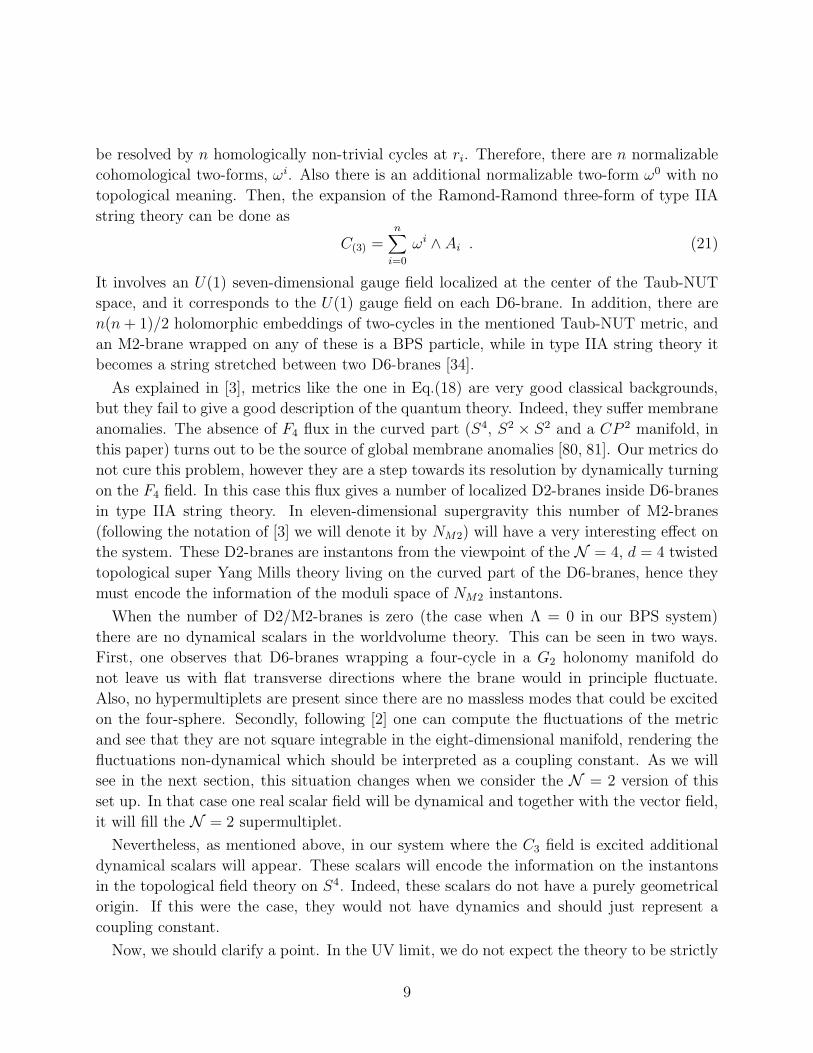
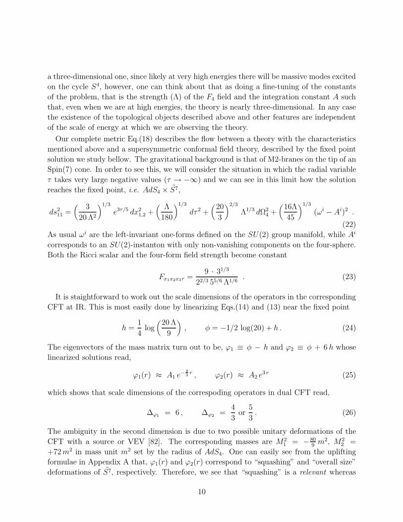
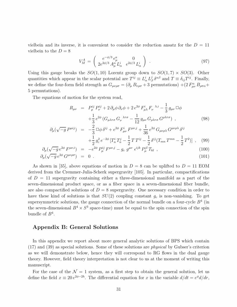
while, of course, Fx1x2x3r = 0. In figure 1 we show the behavior of Fx1x2x3r, 2/3F 2x1x2x3r and

the Ricci scalar R, as a function of τ . We can see how the solid lines are exactly the same

curve up to a minus sign. This graphically reflects the validity of the eleven-dimensional

equations of motion.

-7.5 -5 -2.5 2.5 5 7.5 10tau

-2

-1

1

2

UV Spin7IR f.p.

R

F2

F

Figure 1: Fx1x2x3r, 2/3F 2x1x2x3r (labeled as F 2) and the Ricci scalar R,

as a function of τ .

From this figure, we can also see how both the four-form field strength and the Ricci

scalar go to zero at the UV limit. From the vanishing of the Ricci scalar it shows how the

eleven-dimensional manifold becomes flat at UV, while in the IR limit it is negative, as one

expects from AdS-like spacetimes.

We can understand some aspects of the field theory at the UV regime described by the

metric (20). A very beautiful paper analyzing these kind of aspects is [3]. We can understand

topological objects in the effective 2 + 1-dimensional field theory as follows. From an M-

theory perspective they must correspond to M2 or M5-branes wrapping non-contractible

cycles, that “intersect” the 2+1-dimensional worldvolume. Existence of suitable non-trivial

cycles will signal the possibility of having a given topological defect. For example, a domain

wall will be represented by an M5-brane wrapping a four-cycle, so the existence of domain

walls will be determined by non-triviality of H4(X8, Z) (where X8 is the eight-dimensional

manifold “external” to 2+1 flat directions). Monopoles and instantons will be associated with

H5(X8, Z) and H3(X8, Z) since they will correspond to M5-branes wrapping five-cycles and

membranes wrapping three-cycles. Indeed, there is a correspondence between M-theory and

type IIA string theory degrees of freedom. For instance, if one considers the multi-centered

Taub-NUT metric times a seven-dimensional Minkowski spacetime in eleven dimensions, in

type IIA string theory one can think of that as n+1 parallel D6-branes placed at each center

ri of the Taub-NUT four-dimensional metric. In eleven dimensions the An singularity can

8

be resolved by n homologically non-trivial cycles at ri. Therefore, there are n normalizable

cohomological two-forms, ωi. Also there is an additional normalizable two-form ω0 with no

topological meaning. Then, the expansion of the Ramond-Ramond three-form of type IIA

string theory can be done as

C(3) =n∑

i=0

ωi ∧ Ai . (21)

It involves an U(1) seven-dimensional gauge field localized at the center of the Taub-NUT

space, and it corresponds to the U(1) gauge field on each D6-brane. In addition, there are

n(n+ 1)/2 holomorphic embeddings of two-cycles in the mentioned Taub-NUT metric, and

an M2-brane wrapped on any of these is a BPS particle, while in type IIA string theory it

becomes a string stretched between two D6-branes [34].

As explained in [3], metrics like the one in Eq.(18) are very good classical backgrounds,

but they fail to give a good description of the quantum theory. Indeed, they suffer membrane

anomalies. The absence of F4 flux in the curved part (S4, S2 × S2 and a CP 2 manifold, in

this paper) turns out to be the source of global membrane anomalies [80, 81]. Our metrics do

not cure this problem, however they are a step towards its resolution by dynamically turning

on the F4 field. In this case this flux gives a number of localized D2-branes inside D6-branes

in type IIA string theory. In eleven-dimensional supergravity this number of M2-branes

(following the notation of [3] we will denote it by NM2) will have a very interesting effect on

the system. These D2-branes are instantons from the viewpoint of the N = 4, d = 4 twisted

topological super Yang Mills theory living on the curved part of the D6-branes, hence they

must encode the information of the moduli space of NM2 instantons.

When the number of D2/M2-branes is zero (the case when Λ = 0 in our BPS system)

there are no dynamical scalars in the worldvolume theory. This can be seen in two ways.

First, one observes that D6-branes wrapping a four-cycle in a G2 holonomy manifold do

not leave us with flat transverse directions where the brane would in principle fluctuate.

Also, no hypermultiplets are present since there are no massless modes that could be excited

on the four-sphere. Secondly, following [2] one can compute the fluctuations of the metric

and see that they are not square integrable in the eight-dimensional manifold, rendering the

fluctuations non-dynamical which should be interpreted as a coupling constant. As we will

see in the next section, this situation changes when we consider the N = 2 version of this

set up. In that case one real scalar field will be dynamical and together with the vector field,

it will fill the N = 2 supermultiplet.

Nevertheless, as mentioned above, in our system where the C3 field is excited additional

dynamical scalars will appear. These scalars will encode the information on the instantons

in the topological field theory on S4. Indeed, these scalars do not have a purely geometrical

origin. If this were the case, they would not have dynamics and should just represent a

coupling constant.

Now, we should clarify a point. In the UV limit, we do not expect the theory to be strictly

9

a three-dimensional one, since likely at very high energies there will be massive modes excited

on the cycle S4, however, one can think about that as doing a fine-tuning of the constants

of the problem, that is the strength (Λ) of the F4 field and the integration constant A such

that, even when we are at high energies, the theory is nearly three-dimensional. In any case

the existence of the topological objects described above and other features are independent

of the scale of energy at which we are observing the theory.

Our complete metric Eq.(18) describes the flow between a theory with the characteristics

mentioned above and a supersymmetric conformal field theory, described by the fixed point

solution we study bellow. The gravitational background is that of M2-branes on the tip of an

Spin(7) cone. In order to see this, we will consider the situation in which the radial variable

τ takes very large negative values (τ → −∞) and we can see in this limit how the solution

reaches the fixed point, i.e. AdS4 × S7,

ds211 =

(

3

20 Λ2

)1/3

e3τ/5 dx21,2 +

(

Λ

180

)1/3

dτ 2 +(

20

3

)2/3

Λ1/3 dΩ24 +

(

16Λ

45

)1/3

(ωi − Ai)2 .

(22)

As usual ωi are the left-invariant one-forms defined on the SU(2) group manifold, while Ai

corresponds to an SU(2)-instanton with only non-vanishing components on the four-sphere.

Both the Ricci scalar and the four-form field strength become constant

Fx1x2x3τ =9 · 31/3

22/3 55/6 Λ1/6. (23)

It is staightforward to work out the scale dimensions of the operators in the corresponding

CFT at IR. This is most easily done by linearizing Eqs.(14) and (13) near the fixed point

h =1

4log

(

20 Λ

9

)

, φ = −1/2 log(20) + h . (24)

The eigenvectors of the mass matrix turn out to be, ϕ1 ≡ φ − h and ϕ2 ≡ φ + 6 h whose

linearized solutions read,

ϕ1(r) ≈ A1 e− 4

3r , ϕ2(r) ≈ A2 e

3 r (25)

which shows that scale dimensions of the correspoding operators in dual CFT read,

∆ϕ1= 6 , ∆ϕ2

=4

3or

5

3. (26)

The ambiguity in the second dimension is due to two possible unitary deformations of the

CFT with a source or VEV [82]. The corresponding masses are M21 = −80

9m2, M2

2 =

+72m2 in mass unit m2 set by the radius of AdS4. One can easily see from the uplifting

formulae in Appendix A that, ϕ1(r) and ϕ2(r) correspond to “squashing” and “overall size”

deformations of S7, respectively. Therefore, we see that “squashing” is a relevant whereas

10

“overall size” is an irrelevant deformation in the dual CFT. In [83] the squashing operator,

ϕ1 was identified with the singlet of the isometry group SO(5) × SO(3) of S7 under the

decomposition of (0, 2, 0, 0) of SO(8). Obviously the overall size operator, ϕ2 should be

identified with the singlet of SO(5)×SO(3) inherited from (0, 0, 0, 0) of SO(8). Looking at

the standard tables for mass operators, e.g. in [84], one indeed sees that it is the singlet in the

KK-tower 0+(3) and has M22 = +72m2 and energy ∆ = 6. Note that in our solution (17) we

turned off the squashing deformation, i.e. we set h − φ = const. This is a supersymmetric

hence stable truncation. Since the only relevant deformation in the dual theory is turned off

and we are left with an irrelevant overall size deformation, CFT appears in IR. On the other

hand, in the more general solution of Appendix B where we turn on ϕ1 along with ϕ2, dual

CFT appears in the UV limit, as expected.

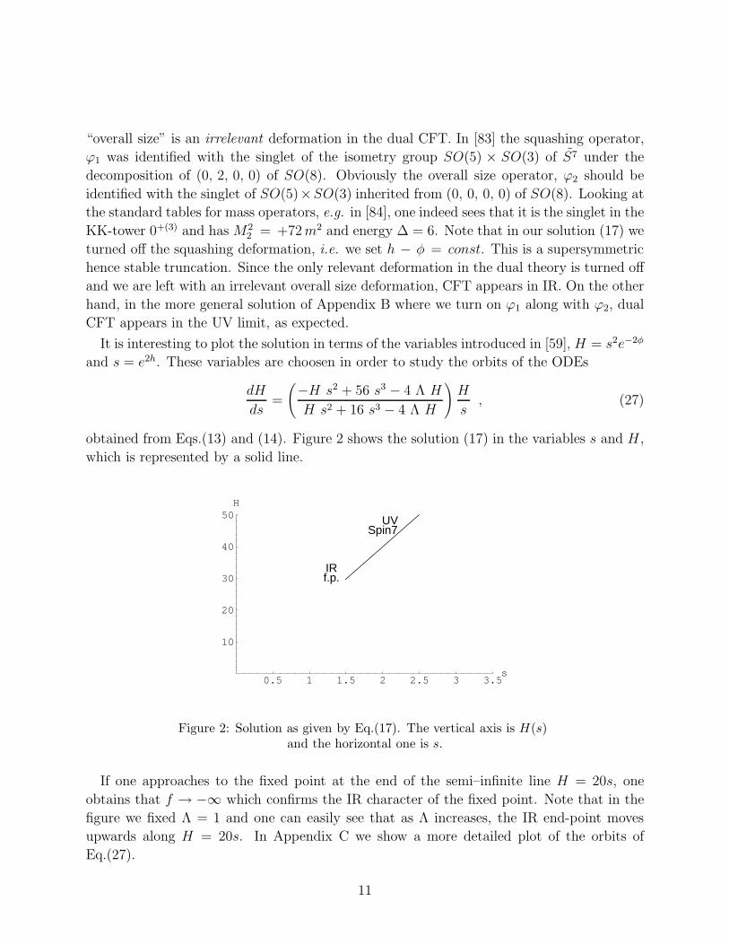
It is interesting to plot the solution in terms of the variables introduced in [59], H = s2e−2φ

and s = e2h. These variables are choosen in order to study the orbits of the ODEs

dH

ds=

(

−H s2 + 56 s3 − 4 Λ H

H s2 + 16 s3 − 4 Λ H

)

H

s, (27)

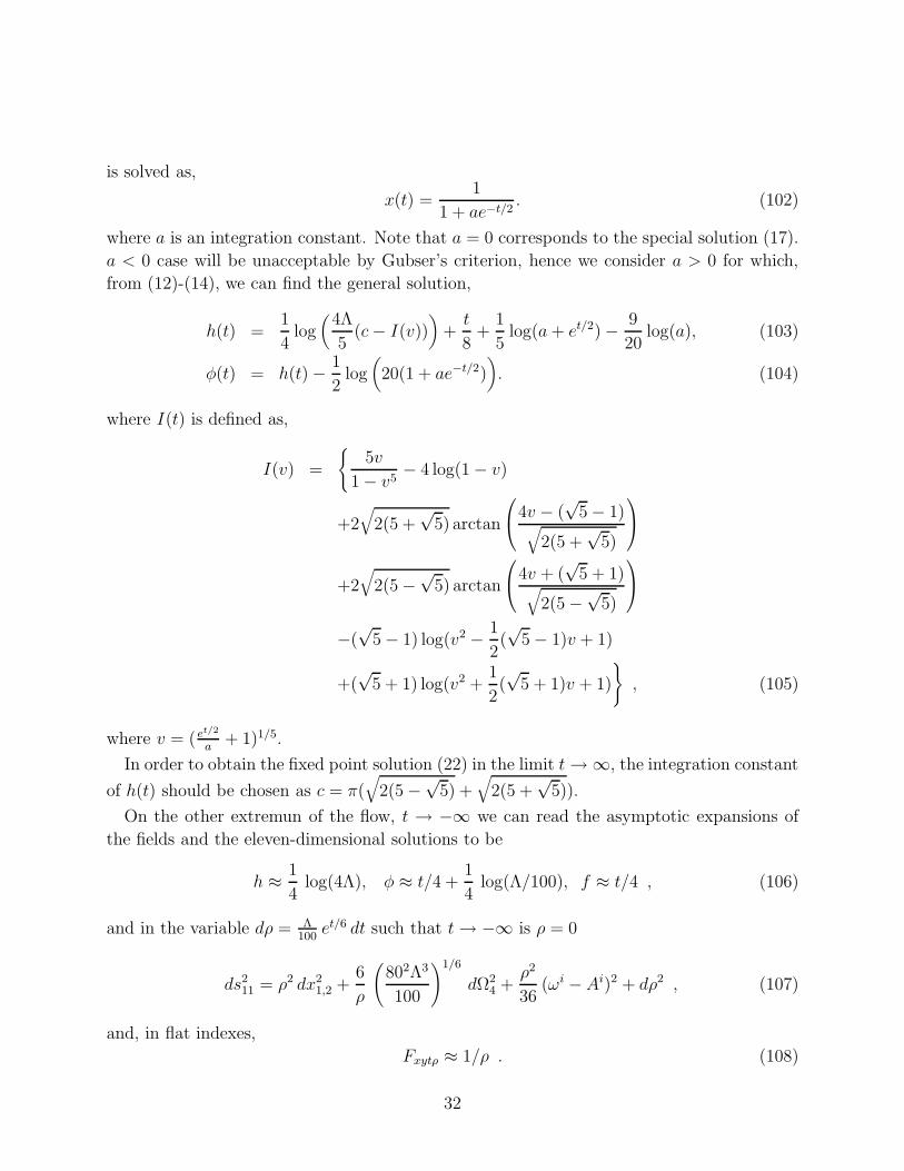
obtained from Eqs.(13) and (14). Figure 2 shows the solution (17) in the variables s and H ,

which is represented by a solid line.

0.5 1 1.5 2 2.5 3 3.5s

10

20

30

40

50H

UVSpin7

IRf.p.

Figure 2: Solution as given by Eq.(17). The vertical axis is H(s)and the horizontal one is s.

If one approaches to the fixed point at the end of the semi–infinite line H = 20s, one

obtains that f → −∞ which confirms the IR character of the fixed point. Note that in the

figure we fixed Λ = 1 and one can easily see that as Λ increases, the IR end-point moves

upwards along H = 20s. In Appendix C we show a more detailed plot of the orbits of

Eq.(27).

11

The conclusion is that at UV the metric asymptotically corresponds to a three-dimensional

Minkowski spacetime times an Spin(7) holonomy manifold. Then, it flows to the IR fixed

point (AdS4 × S7) along H = 20s .

One can consider more general solutions to the BPS equations (12)–(14) by turning on

one more degree of freedom, namely allowing also the difference φ(τ) − h(τ) in Eq.(17) to

be τ -dependent. This solution and similar generalizations of the solutions of next section

are obtained in Appendix B. They typically suffer from curvature singularities which render

the field theory interpretation difficult. However, we present some cases where curvature

singularities at IR are acceptable by Gubser’s criterion [85].

5 From CY4 folds to AdS spaces and FT duals

5.1 D6-branes wrapping cycles inside CY3 folds

Now, we will study a system in an analogous way as in the previous section, but preserv-

ing twice the number of supersymmetries compared to the above E2,1 × Spin(7) example.

Therefore, we will consider a D2-D6 system where the D6-branes are wrapping a four-cycle

of constant curvature which, in the present case, will be S2 × S2. At the UV limit this four-

cycle is inside a CY3 fold, and the number of supercharges preserved by this configuration

becomes 4, thus leading to an N = 2 SYM theory in three dimensions. On the other hand, in

the IR limit we will obtain an eleven-dimensional metric corresponding to M2-branes on the

tip of cone based over Q1,1,1, an Einstein-Sasakian manifold. This represents the gravity dual

of a three-dimensional N = 2 SCFT. In this section we want to argue that special holonomy

manifold is a cone over a CY3 fold. Furthermore, we will see that it can be resolved in two

possible ways, both of them require to turn on an additional degree of freedom in the gauged

supergravity. First way of resolution preserves the zero curvature of the configuration and

leads to special holonomy manifolds representing duals of three-dimensional N = 2 gauge

theories with a mass gap, whereas the other way turns on a degree of freedom in the lower

dimensional supergravity leading to a configuration of the form AdS4×Y7 in M-theory. Here

our interest concentrates on the latter type of resolutions, that as in the previous section,

leads to different physical effects.

Let us start by considering the theory with D2 and D6-branes. Since we want to wrap

the D6-branes in a four-cycle of the form S2 × S2, we have to choose an eight-dimensional

metric of the form

ds28 = e2f dx2

1,2 + dr2 + e2h(

dθ21 + sin2 θ1 dϕ

21 + dθ2

2 + sin2 θ2 dϕ22

)

, (28)

together with an Abelian gauge field A(3) = cos θ1 dϕ1 + cos θ2 dϕ2. It means that now the

normal bundle of S2 × S2 is U(1). Therefore, in order to define Killing spinors by means of

twisting, we must break the SU(2) group down to U(1). This is achieved by turning on the

12

field λ(r) in the eight-dimensional gauged supergravity. Indeed, this field makes a distinction

between the three directions of the S3 “external” to the branes system, thus leading to a

symmetry breaking SU(2) → U(1). For this reason, in gauged supergravity we choose a

“vielbein” of the form Liα = diag(eλ, eλ, e−2λ), that generates T 11 = T 22 = e2λ, T 33 = e−4λ,

as well as,

P 11µ = P 22

µ = ∂µλ , P 33µ = −2∂µλ , (29)

Q12µ = −g A(3)

µ , Q13µ = g cosh(3λ)A(2)

µ , Q32µ = g sinh(3λ)A(1)

µ . (30)

As before, we have a G4 field (in flat index notation)

Gx1x2x3r = Λ e−2φ−4h . (31)

After plugging it into the supersymmetric variations of fermions, it produces the following

BPS equations,

f ′ = −1

3eφ−2h−2λ +

1

24e−φ (e−4λ + 2e2λ) +

Λ

2e−4h−φ , (32)

φ′ = −eφ−2h−2λ +1

8e−φ (e−4λ + 2 e2λ) − Λ

2e−4h−φ , (33)

h′ =2

3eφ−2h−2λ +

1

24e−φ (e−4λ + 2e2λ) − Λ

2e−4h−φ , (34)

λ′ =2

3eφ−2h−2λ − 1

12e−φ (−2e−4λ + 2e2λ) . (35)

When Λ = 0 this system coincides with the one in ref.[13] 4.

Indeed, in this case (Λ = 0), a simple solution can be easily found

λ =1

6log(2), eh =

3r

4√

2, φ = h− 7

6log(2), 3f = φ , (36)

that lifted to eleven dimensions, and after a suitable change of radial variable, reads as

ds211 = dx2

1,2 + dρ2 +

ρ2

8

(

dΩ21 + dΩ2

2 + dΩ23 +

1

2(dψ + cosα dβ − cos θ1 dφ1 − cos θ2dφ2)

2)

. (37)

The metric has a singularity at ρ = 0. We are mainly interested in resolving the singularity

by turning on M2-branes. However, as an aside, let us consider other ways of resolution

which do not render the field theory ending in a conformal point as follows. In gauged

supergravity it can be done giving the field λ a radial dependence. Indeed, by allowing λ to

4We thank the authors for clarifying a missprint in their original version.

13

be variable we can obtain a more general solution that can be continued towards the IR. By

defining a function w and changing variables like

w(ρ) =3ρ4 + 8ρ2 + 6 + Cρ−4

6(ρ2 + 1)2, dr = dρ

(

ρ2

16w5/3

)1/4

, (38)

we have a solution that reads

e−6λ = w(ρ), e2/3φ =ρw1/6

4,

e2h =(ρ2 + 1) ρw1/6

16, f =

1

3φ . (39)

This generates an eleven-dimensional metric as

ds211 = dx2

1,2 +1

w(ρ)dρ2 +

ρ2

4dΩ2

1

+(ρ2 + 1)

4(dΩ2

2 + dΩ23) +

ρ2w(ρ)

4(dψ + cosα dβ − cos θ1 dφ1 − cos θ2 dφ2)

2) ,

(40)

corresponding to the metric for C2 bundle over CP 1 × CP 1. In the case in which the

integration constant C = 0 we recover the solution given in [13, 14], in the case of non-zero

C this seems to be another possible resolution.

Now, let us turn back to our main interest, resolution by dynamically turning on F4. To

this end, we will analyze a different kind of solutions of the above BPS equations, with a

non-zero parameter Λ and study their holographic RG flows as in the previous section.

A solution driving the flow from E2,1 × CY 4 to AdS4 ×Q1,1,1

Since in this case there is an additional degree of freedom, a suitable change of variable,

as compared to Eq.(16), is

dr = eφ+4λ dτ . (41)

A solution of the system (32)-(35) is

h(τ) =1

4log

(

28/3 Λ

3+ Ae3τ/2

)

, φ(τ) = −7/6 log(2) + h(τ) ,

f(τ) =τ

2− 1

4log

(

28/3 Λ + 3Ae3τ/2)

, λ =1

6log(2) , (42)

where A is an integration constant. The corresponding eleven-dimensional metric is given

by

ds211 =

27/9 × 31/6 × eτ

(3Ae3τ/2 + 28/3 Λ)2/3dx2

1,2

14

+1

22/9 × 31/3(3Ae3τ/2 + 28/3 Λ)1/3 dτ 2 +

27/9

31/3(3Ae3τ/2 + 28/3 Λ)1/3 ×

(

dΩ21 + dΩ2

2 + dΩ23 +

1

2(dψ + cosα dβ − cos θ1dφ1 − cos θ2dφ2)

2)

. (43)

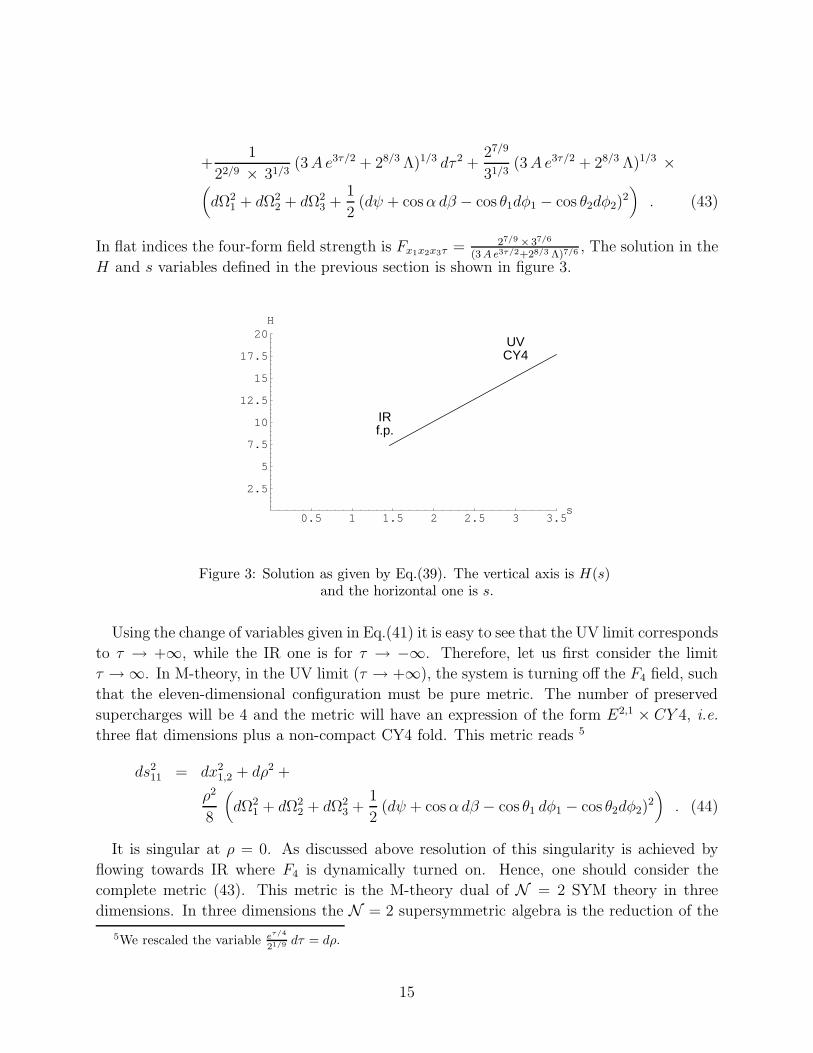
In flat indices the four-form field strength is Fx1x2x3τ = 27/9 × 37/6

(3 A e3τ/2+28/3 Λ)7/6 , The solution in the

H and s variables defined in the previous section is shown in figure 3.

0.5 1 1.5 2 2.5 3 3.5s

2.5

5

7.5

10

12.5

15

17.5

20H

UVCY4

IRf.p.

Figure 3: Solution as given by Eq.(39). The vertical axis is H(s)and the horizontal one is s.

Using the change of variables given in Eq.(41) it is easy to see that the UV limit corresponds

to τ → +∞, while the IR one is for τ → −∞. Therefore, let us first consider the limit

τ → ∞. In M-theory, in the UV limit (τ → +∞), the system is turning off the F4 field, such

that the eleven-dimensional configuration must be pure metric. The number of preserved

supercharges will be 4 and the metric will have an expression of the form E2,1 × CY 4, i.e.

three flat dimensions plus a non-compact CY4 fold. This metric reads 5

ds211 = dx2

1,2 + dρ2 +

ρ2

8

(

dΩ21 + dΩ2

2 + dΩ23 +

1

2(dψ + cosα dβ − cos θ1 dφ1 − cos θ2dφ2)

2)

. (44)

It is singular at ρ = 0. As discussed above resolution of this singularity is achieved by

flowing towards IR where F4 is dynamically turned on. Hence, one should consider the

complete metric (43). This metric is the M-theory dual of N = 2 SYM theory in three

dimensions. In three dimensions the N = 2 supersymmetric algebra is the reduction of the

5We rescaled the variable eτ/4

21/9dτ = dρ.

15

N = 1 in four dimensions. The role of the central charge is played by the four component

of the momentum. As in the higher dimensional case, the R-symmetry group is U(1)R.

As usual, scalars in the vector superfield parameterize the Coulomb branch of the theory.

In this case some fundamental hypermultiplets exist in the Lagrangian which will describe

the Higgs branch. In our case, we expect a dynamical scalar field coming from fluctuations of

the metric. Another way of understanding the presence of this dynamical scalar is by noticing

that D6-branes wrap an S2 × S2 cycle inside a complex three-dimensional CY space. Thus,

there will be one free direction (codimension one) in contrast to the G2 case analyzed in

the previous section. This direction is interpreted as a scalar field describing the Coulomb

branch of the theory.

In addition, due to the presence of D2-branes, or due to the C3 field in M-theory, some

other scalar modes will have dynamics on the 2 + 1-dimensional worldvolume.

In a non-Abelian theory, when we move into the Coulomb branch, we can dualize the

vectors to scalars in linear multiples Aµ → γ and the Coulomb branch is parametrized by

the complex scalar Φ = ϕ+ iγ, like in four dimensions, this is the factor that appears when

the instanton contributions are taken into account. In the case in which we have fundamental

hypermultiplets, the interaction term is typically of the form

V ∼∫

d2θd2θQeVQ . (45)

So, a bosonic term will be of the form qϕq, this means that in general, the Coulomb branch

and the Higgs branch will be disconnected. Nevertheless, there are situations in which we

have a mixing of Coulomb and Higgs branches. We will not discuss these cases here, since

our configurations will not have hypermultiplets. As it was studied by Affleck, Harvey and

Witten, the instantons that are associated with Π2(G) are only present when we have a non-

Abelian gauge group and we consider the Coulomb branch, so Π2(G/U(1)r) = Zr. These

instantons generate a superpotential that in the large N limit goes to W ∼ e−N , so we

cannot see it in a supergravity approximation. This is the reason why a brane probe of our

configuration will lead to a 2-dimensional flat Coulomb branch. It would be of much interest,

to find dual gravity configurations to theories with fundamental hypermultiplets.

On the other limit of the flow, i.e. when τ → −∞, one obtains the metric

ds211 = eξρ dx2

1,2 + dρ2 + 2

(

4|Λ|3

)1/3

×(

dΩ21 + dΩ2

2 + dΩ23 +

1

2(dψ + cosα dβ − cos θ1 dφ1 − cos θ2 dφ2)

2)

, (46)

where as before, dΩ2i denotes the line element over a two-sphere6. In addition, one has a

four-form field of the form Fx1x2x3τ = 27/9 37/6

(28/3 Λ)7/6 . The manifold in Eq.(46) is AdS4×Q1,1,1 and

6We rescaled the variable τ as 21/3 Λ1/6

31/6dτ = dρ.

16

the conformal field theory to which this manifold is dual is well-known. Indeed, the manifold

Q1,1,1 has been well studied in the past. The isometries of this space are SU(2)3 ×U(1) and

are in correspondence with the global symmetries of the CFT. The KK modes on Q1,1,1 were

worked out in [86]. It contains short and long multiplets of Osp(2|4).

By linearizing the BPS equations (33 - 35) near the fixed point, one can work out the

scale dimensions of the operators dual to the eigenvectors of the mass matrix which are

combinations of φ, h and λ. Dimensions turn out to be,

∆1 = 6 , ∆2, 3 =3

2±√

31

12. (47)

Note, however, that in Eq.(42) latter two of the eigenvectors are turned off by requiring λ =

const. and h − φ = const.. Thus, as in the previous example, one is left with an irrelevant

“overall size” deformation of Q1,1,1 with dimension ∆ = 6 and mass, M2 = 72. Therefore

the dual CFT is at IR. Solutions obtained by turning on more eigenvectors are presented

in Appendix B, for which AdS geometry appears at UV, as one expects. KK spectrum of

AdS4 × Q1,1,1 compactification was partially worked out in [87] and one indeed finds that

the “overall size” deformation is a singlet of the bosonic isometry SU(2) × SU(2) × SU(2)

and U(1) R-symmetry together with (in our normalization conventions) ∆ = 6 and mass,

M2 = 72.

The CFT dual to the metric (46) corresponds to the one in an M2-brane on the tip of a

cone on the seven-dimensional manifold [88, 89, 90, 91, 92, 93, 94, 95]. This gauge theory

has a moduli space of vacua isomorphic to Q1,1,1.

Like other CFT’s the theory has a Coulomb branch described by fields in the vector

multiplet and a Higgs branch described by fields in chiral multiplets. Working out the

theory whose Higgs branch is dual to the conifold above, one finds that fundamental fields

are doublets with respect to the flavour group SU(2)3 : Ai, Bi, Ci with i = 1, 2, i.e., the

fields transform as Ai = (2, 1, 1), Bi = (1, 2, 1), Ci = (1, 1, 2) under the flavour group.

The gauge theory has the color symmetry SU(N) × SU(N) × SU(N), with elementary

degrees of freedom transforming in the fundamental and anti-fundamental representation

of the SU(N)′s, namely Ai = (N, N, 1), Bi = (1, N, N), Ci = (N, 1, N). These fields have

conformal weight c = 1/3, hence one can construct gauge invariant operators of the form

X ijk = AiBjCk , (48)

out of them. These eight operators are singlets under the global symmetries and have

conformal weight equal to one.

One important point is the comparison of the KK modes on the Q1,1,1 manifold and the

spectrum of hypermultiplets in the CFT. The spectrum of the Laplacian in Q1,1,1 is computed

and one can associate it with a chiral multiplet in the (k/2, k/2, k/2) representation of SU(2)3

with dimension E = k. Therefore, it is natural to make a correspondence with composite

17

operators of the form Tr(ABC)k with symmetrized SU(2) indices. This agrees with the

gauge theory.

Nevertheless, there are some operators in gauge theory–like those where the SU(2) indices

are not symmetrized–that do not have a KK analog. One would think that a superpotential

can be generated in such a way to get rid of those states as in the case of T 1,1, but this is not

the case. Indeed, we can see from a gauge theory perspective that the potential that should

do the job

V ∼ [(|A1|2 + |A2|2 − |C1|2 − |C2|2)2 + (|B1|2 + |B2|2 − |A1|2 − |A2|2+)2

+(|C1|2 + |C2|2 − |B1|2 − |B2|2)2] , (49)

vanishes due to the fact that it is exactly the (Higgs branch) description of the manifold

Q1,1,1. So, the potential does not solve the problem and one needs to assume that these

unwanted colored degrees of freedom are not chiral primaries.

One can also find the presence of a baryonic operator essentially corresponding to wrapping

an M5-brane on a five-cycle inside the eight-cone. The operators corresponding to baryons are

of the form det[A], det[B], det[C]. Since our manifoldQ1,1,1 has Betti numbers b2, b5 different

from zero, there is another U(1) under which only non-perturbative states will be charged.

In our case, the baryonic symmetry acts on the fundamental fields as Ai = (1,−1, 0), Bi =

(0, 1,−1), Ci = (−1, 0, 1), therefore we can see that gauge invariant operators X are not

charged under baryon number. One can compute the dimension of the baryonic operator

by computing the mass of an M5-brane wrapping a five-cycle inside the cone. This mass in

the case of a supersymmetric cycle, coincides with the volume of the cycle. In our case the

five-cycle is a U(1) fibre over S2×S2 and since our manifold is a U(1) → S2×S2×S2 we have

three different supersymmetric cycles that are associated with the three operators defined

above. Each cycle is supersymmetric as we can see from the twisting condition described

above. The volume of the cycle, can be computed to be proportional to N/3 thus confirming

the fact that each operator A,B,C have dimension 1/3. If the M5-brane wraps a three-cycle,

the object is interpreted as a domain wall of the CFT.

5.2 The case of N = 3 supersymmetry: from HK to N0,1,0

Here, we will briefly comment on the case where the D6-branes are wrapping a four-cycle that

preserves N = 3 supersymmetry. The set up is very similar to the previous examples, except

we take the four-cycle to be a CP 2 manifold. We choose a metric (using as coordinates ξ

and the three angles in the left-invariant forms σi)

ds2CP2 = dξ2 +

1

4sin2 ξ (σ2

1 + σ22 + cos2ξ σ2

3) . (50)

18

The gauge field which provides the twisting preserving six supercharges is given by

A(i) = cos ξ σ(i), A(3) =1

2(1 + cos2 ξ)σ(3) . (51)

A solution of the BPS equations lifted to eleven dimensions reads

ds211 =

dx21,2

(

1 + Br6

)2/3+(

r6 +B)1/3

ds2CP2+2

(

B

r6+ 1

)1/3

dr2+r2

2

(

B

r6+ 1

)1/3

(ωi−Ai)2 (52)

together with the four-form field strength

Fxyzr =3B

(B + r6)7/6, (53)

written in flat indices, where B is a constant. Therefore, the metric (52) represents a

holographic RG flow from E2,1 × HK (hyperKahler) at UV to AdS4 × N0,1,0 at IR. The

isometry group of N0,1,0 is SU(3) × SU(2) while its holonomy is SU(2).

As it is known, an N = 3 supersymmetric gauge theory has the field content of an N = 4

supersymmetric gauge theory, plus an interaction that respects three out of the four spinors.

It was shown by Kapustin and Strassler [96] that for the Abelian case, the ways of breaking

N = 4 down to N = 3 supersymmetry are either by adding a Chern Simons term or with a

mass term for a chiral superfield Y I in the adjoint representation of the gauge group.

In our case, we have a supergravity solution of the form AdS4 × N0,1,0. The dual gauge

theory in the IR limit will have a gauge group SU(N) × SU(N) and a flavor group SU(3).

There will be two hypermultiplets, u1, u2 and v1, v2 transforming in the (3, N, N) and

(3, N , N) representations and two chiral multiplets, Y(1), Y(2) in the adjoint representation of

SU(N). There is a superpotential of the form

V ∼ gi Tr(Y(i) ~u · ~v) + αi Tr(Y(i) Y(i)) , (54)

where gi are the gauge couplings of each SU(N) group and αi are the Chern Simons coeffi-

cients. Interesting aspects of this theory, like the KK spectrum of the compactifications and

different checks of the duality have been studied in [97, 98].

6 Penrose limits and pp-waves

In this section we will show how to obtain the pp-waves in the Penrose limit for the IR region

of the supergravity solutions described in sections 4 and 5.

We will focus on the solutions with N = 2 and N = 3 supersymmetry and we will add a

brief description of the N = 1 case near the end of the section.

19

The interest of taking the Penrose limit is based on the fact that it could be possible to

define following [37] a Matrix model to check the correlation between the gravity and the

gauge theory side. We postpone the checks of this correlations for a future publication, here

we will only concentrate on the gravity aspects.

Penrose limit of the AdS × Einstein-Sasakian manifold

The Einstein metric of AdS4 ×Q1,1,1 can be written as

ds211 = ds2

AdS4+ ds2

Q1,1,1 , (55)

where

ds2AdS4

= R2 (−dt2 cosh2 ρ+ dρ2 + sinh2 ρ dΩ22) , (56)

and

ds2Q1,1,1 = µ2R2 (dθ2

1 + sin2 θ1 dφ21 + dθ2

2 + sin2 θ2 dφ22 + dθ2

3 + sin2 θ3 dφ23 +

1

2(dψ + cos θ1 dφ1 + cos θ2 dφ2 + cos θ3 dφ3)

2) . (57)

Where µ is the relation between the radii of AdS4 and Q1,1,1. Topologically Q1,1,1 is a

U(1) bundle over S2 × S2 × S2, so that it can be parametrized by (θ1, φ1), (θ2, φ2) and

(θ3, φ3) coordinates over each S2, respectively, while the period of the Hopf fiber coordinate

ψ is 4π. The SU(2)1 × SU(2)2 × SU(2)3 × U(1) isometry of Q1,1,1 is identified with the

SU(2)1×SU(2)2×SU(2)3 global symmetry and U(1)R symmetry of the dual SU(N) N = 2

SCFT in three dimensions.

Now, the idea is to obtain a certain scaling limit around a null geodesic in AdS4 ×Q1,1,1.

This rotates the ψ coordinate of Q1,1,1 in correspondence with the U(1)R symmetry of the

dual SCFT. Moreover, the changes in the angles φ1, φ2 and φ3 generate an U(1)1 ×U(1)2 ×U(1)3 ⊂ SU(2)1 × SU(2)2 × SU(2)3 isometry. In the SCFT side this is generated by

the dual Abelian charges Q1, Q2 and Q3, which are the Cartan generators of the global

SU(2)1 × SU(2)2 × SU(2)3 symmetry group of the field theory.

Thus we define new coordinates

x+ =1

2

(

t+µ√2(ψ + φ1 + φ2 + φ3)

)

, (58)

x− =R2

2

(

t− µ√2(ψ + φ1 + φ2 + φ3)

)

. (59)

Note the scaling in the latter equation by R2. We will consider a scaling limit around

ρ = θ1 = θ2 = θ3 = 0 in the metric above, such that when we take the limit R→ ∞ we also

scale the coordinates as follows

ρ =r

R, θ1 =

ζ1R, θ2 =

ζ2R, θ3 =

ζ2R. (60)

20

Therefore, the Penrose limit of the AdS4 ×Q1,1,1 metric is given by

ds211 = −4 dx+ dx− +

3∑

i=1

(dri dri − ri ri dx+ dx+) +3∑

i=1

(µ2dζ2i + µ2ζ2

i dφ2i −

µ√2ζ2i dφi dx

+) .

(61)

Changing to the complex coordinates zj = ζj eiφj one obtains

ds211 = −4 dx+ dx−+

3∑

i=1

(dri dri−ri ri dx+ dx+)+3∑

j=1

(µ2dzj dzj +iµ

2√

2(zj dzj−zj dzj) dx

+) .

(62)

This metric has a covariantly constant null Killing vector ∂/∂x−, and therefore is a pp-

wave metric having a decomposition of R9 as R3 × R2 × R2 × R2. Three-dimensional

Euclidean space is parametrized by ri, while R2 ×R2 ×R2 is parametrized by zj above. In

addition, the background has a constant F+x1x2r. The symmetries of this configuration are

the SO(3) rotations in R3 and U(1) × U(1) × U(1) symmetry related to the R2 ×R2 × R2

rotations. We choose this particular Penrose limit due to the fact that these U(1)’s are

representing the symmetries of the gauge theory dual to this background. From the dual

field theory viewpoint, the SO(3) isometry is a subgroup of the SO(2, 3) conformal group.

U(1) × U(1) × U(1) rotational charges J1, J2 and J3 correspond to differences between

U(1) × U(1) × U(1) charges Q1, Q2 and Q3 and the U(1)R charge. Indeed from the field

theory side, it is expected to deal with operators with large U(1)R symmetry charge J , being

the charges Q1, Q2 and Q3 also scaled as√N like J , while the corresponding rotational

charges Ji’s would remain finite.

After an U(1) × U(1) × U(1) rotation in the R2 ×R2 × R2 plane as

zj = ei√

2 x+/(4 µ) wj, zj = e−i√

2 x+/(4 µ) wj, (63)

one obtains a metric that after suitable rescalings of its variables turns out to be

ds211 = −4 dx+ dx− −

(

(

µ

6

)2

~r 23 +

(

µ

3

)2

~y 26

)

dx+ dx+ + d~r 23 + d~y 2

6 , (64)

where yj are the 6 coordinates on R2 × R2 × R2. The above metric corresponds to the

maximally supersymmetric pp-wave solution of AdS4 × S7. It means that the dual SCFT is

N = 8, SU(N) super Yang Mills theory in three dimensions. This shows the enhancement of

supersymmetry analogous to the ones obtained in [41, 42, 44]. This fact might be interpreted

as a hidden N = 8 supersymmetry which was already present in the corresponding subsector

of the dual N = 2 SCFT.

Penrose limit of the AdS ×N0,1,0 manifold

The Einstein metric of AdS4 ×N0,1,0 can be written as

ds211 = ds2

AdS4+ ds2

N0,1,0 , (65)

21

where we again use

ds2AdS4

= R2 (−dt2 cosh2 ρ+ dρ2 + sinh2 ρ dΩ22) , (66)

while

ds2N0,1,0 = µ2R2 (dζ2 +

sin2 ζ

4(dθ2 + sin2 θ dφ2 + cos2 ζ (dψ + cos θ dφ)2) +

1

2(cos γ dα + sin γ sinα dβ − cos ζ (cosψ dθ + sinψ sin θ dφ))2 +

1

2(− sin γ dα+ cos γ sinα dβ − cos ζ (− sinψ dθ + cosψ sin θ dφ))2 +

1

2(dγ + cosα dβ − 1

2(1 + cos2 ζ) (dψ + cos θ dφ))2) . (67)

Where µ is the relation between the AdS4 and N0,1,0 radii. Again, the idea is to obtain a

certain scaling limit around a null geodesic in AdS4 ×N0,1,0. In this case we can define the

coordinates

x+ =1

2

(

t+µ√2(γ + β − ψ/2 − φ/2)

)

, (68)

x− =R2

2

(

t− µ√2(γ + β − ψ/2 − φ/2)

)

. (69)

We will consider a scaling limit around ρ = θ = α = 0 and ζ = π/2 in the metric above, so

that when we take the limit R → ∞ we also scale the coordinates as

ρ =r

R, ζ =

π

2+x

R, α =

z

R, θ =

y

R. (70)

Therefore, after some appropriate redefinitions of coordinates, the Penrose limit of the AdS4×N0,1,0 metric is given by

ds211 = −4 dx+ dx− +

3∑

i=1

(dri dri − ri ri dx+ dx+) + µ2 ( z2 dβ2 + y2 dφ2 + x2 dψ2) +

µ2 (dx2 + dy2 + dz2) −√

2µ dx+ ( z2 dβ + y2 dφ+ x2 dψ) , (71)

where we have changed ψ + φ→ ψ.

Using the redefinitions

x = ζ1, y = ζ2, z = ζ3, (72)

and

ψ = φ1, φ = φ2, β = φ3, (73)

together with a further rescaling, this metric becomes exactly Eq.(61). Therefore, we can

follow a similar path defining complex coordinates, etc., obtaining that the Penrose limit of

22

AdS4 ×N0,1,0 reduces to the same pp-wave as the corresponding one of AdS4 × S7. Hence,

we might conclude that likely there is a hidden N = 8 supersymmetry which was already

present in the corresponding subsector of the dual N = 3 SCFT.

Penrose limit of the AdS × squashed seven-sphere

Finally, we would like to add some comments on the case of the Spin(7) holonomy manifold,

that is our solution preserving N = 1 supersymmetry. This case is analogous to the Penrose

limit for the gravity solution of D5-branes on the resolved conifold, that has been worked

out in [42] 7.

The Einstein metric of AdS4 × S7 can be written as

ds211 = ds2

AdS4+ ds2

S7 , (74)

where as before we have

ds2AdS4

= R2 (−dt2 cosh2 ρ+ dρ2 + sinh2 ρ dΩ22) , (75)

while

ds2S7 = µ2

(

dΩ24 +

1

5(ωi − Ai)

)

, (76)

where µ stands for the relation between AdS and squashed seven-sphere radii, and the factor

1/5 comes from the relation between S4 and SU(2)-group manifold radii. We remind that

the isometries of S7 are SO(5) × SU(2).

Indeed, we can proceed in the following way, we rescale the coordinates such that the part

coming from the four-sphere reads

dΩ24 ≈

dτ 2

R2+

τ 2

4R2dΩ2

3 , (77)

that is an R4 space. This rescaling includes ρ → r/R, θ → y/R and α → z/R, where the

angles are used to define the left-invariant one forms and the precise definition is given in

Appendix D.

In this coordinates the gauge field will be approximated by Ai ≈ (1 − τ2

R2 ) σi. In the limit

of large R, the term in the metric describing the fibration between the coordinates of the

three-sphere and the four-sphere will basically consist of two parts. After a suitable change

of variables, the term coming from (ωi − σi)2 will contribute to (dx+ − dx−/R2)2 and a flat

two-dimensional space. The second term in the metric (77) proportional to τ will contribute

with a term of the form τ 2/R2dx+dφ. After a similar rescaling as the one for the N = 2 case

is done, it will add a mass term for two of the flat directions, and we obtain a metric that

looks very similar to Eq.(61).

7We thank Jaume Gomis for explanations on this respect.

23

7 RG flows from gauged supergravity in 6 dimensions

In this section we will present other Holographic RG flow examples obtained from F (4)

gauged supergravity [99] in 6 dimensions. These will be of interest since uplifting of these

solutions to massive IIA supergravity is known [52]. The bosonic Lagrangian is

e−1 L(6)B = −1

4R + (∂µϕ)(∂µϕ) − V (ϕ) , (78)

where we set the Abelian, non-Abelian and the two-index tensor gauge fields to zero. The

dilaton potential is given by

V (ϕ) = −1

8(g2 e2ϕ + 4mg e−2ϕ −m2 e−6ϕ) , (79)

where g is the non-Abelian coupling constant and m becomes the mass of Bµν field via Higgs

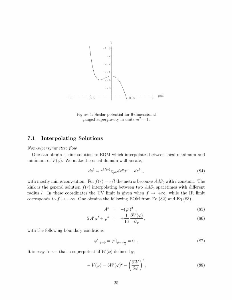
mechanism [99]. Figure 4 shows the dilaton potential. Without loss of generality one can

set g = 3m which will yield a supersymmetric background at the maximum of V at ϕ = 0.

At the two extrema of the potential,

ϕmin = −1

4log(3), V (ϕmin) = −3

√3

2m2 , (80)

and,

ϕMax = 0, V (ϕMax) = −5

2m2 . (81)

which correspond to AdS6 solutions with curvatures RMin = 9√

3m2 and RMax = 15m2,

respectively. The Euler-Lagrange equations are

0 = Rµν − 4∂µϕ∂νϕ+ gµν V (ϕ) , (82)

0 = −22ϕ− ∂V

∂ϕ. (83)

These fixed-point solutions can be lifted to massive type IIA string theory using the up-

lifting procedure given by [52] where the Romans’ F(4) gauged supergravity in 6 dimensions

is obtained from a consistent warped S4 reduction of massive type IIA string theory.

24

-1 -0.5 0.5 1phi

-2.8

-2.6

-2.4

-2.2

-2

-1.8

V

Figure 4: Scalar potential for 6-dimensionalgauged supergravity in units m2 = 1.

7.1 Interpolating Solutions

Non-supersymmetric flow

One can obtain a kink solution to EOM which interpolates between local maximum and

minimum of V (φ). We make the usual domain-wall ansatz,

ds2 = e2f(r) ηµνdxµxν − dr2 , (84)

with mostly minus convention. For f(r) = r/l the metric becomes AdS6 with l constant. The

kink is the general solution f(r) interpolating between two AdS6 spacetimes with different

radius l. In these coordinates the UV limit is given when f → +∞, while the IR limit

corresponds to f → −∞. One obtains the following EOM from Eq.(82) and Eq.(83).

A′′ = −(ϕ′)2 , (85)

5A′ ϕ′ + ϕ′′ = +1

16

∂V (ϕ)

∂ϕ, (86)

with the following boundary conditions

ϕ′|φ=0 = ϕ′|φ=− 1

4

= 0 . (87)

It is easy to see that a superpotential W (φ) defined by,

− V (ϕ) = 5W (ϕ)2 −(

∂W

∂ϕ

)2

, (88)

25

exists but does not have two extrema. Hence the kink interpolating between two AdS6

solutions will necessarily be non-supersymmetric. In this case, one has to solve the second

order EOM given above. The solution corresponds to flowing towards left from the origin in

figure 4. We could not find an analytic solution mostly due to the lack of supersymmetry

along the flow, however a numerical solution can be obtained. A similar study of an RG flow

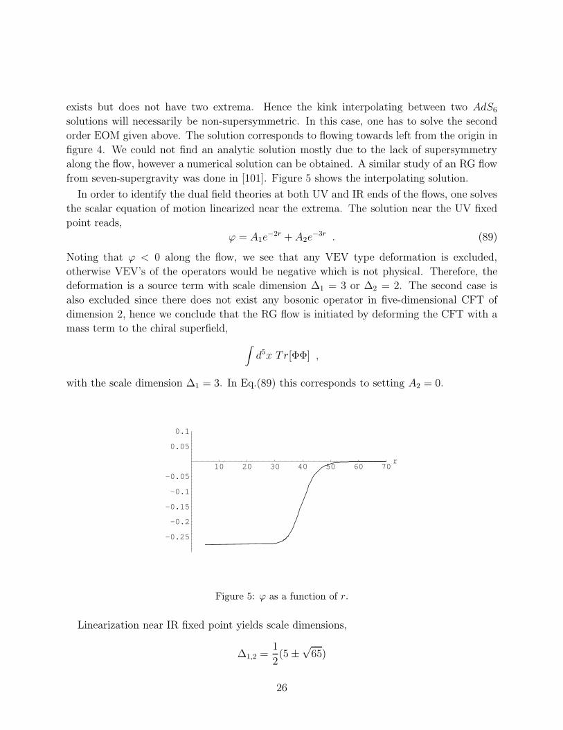
from seven-supergravity was done in [101]. Figure 5 shows the interpolating solution.

In order to identify the dual field theories at both UV and IR ends of the flows, one solves

the scalar equation of motion linearized near the extrema. The solution near the UV fixed

point reads,

ϕ = A1e−2r + A2e

−3r . (89)

Noting that ϕ < 0 along the flow, we see that any VEV type deformation is excluded,

otherwise VEV’s of the operators would be negative which is not physical. Therefore, the

deformation is a source term with scale dimension ∆1 = 3 or ∆2 = 2. The second case is

also excluded since there does not exist any bosonic operator in five-dimensional CFT of

dimension 2, hence we conclude that the RG flow is initiated by deforming the CFT with a

mass term to the chiral superfield,

∫

d5x Tr[ΦΦ] ,

with the scale dimension ∆1 = 3. In Eq.(89) this corresponds to setting A2 = 0.

10 20 30 40 50 60 70r

-0.25

-0.2

-0.15

-0.1

-0.05

0.05

0.1

Figure 5: ϕ as a function of r.

Linearization near IR fixed point yields scale dimensions,

∆1,2 =1

2(5 ±

√65)

26

which shows that the source term acquires an anomalous dimension. This is of course ex-

pected in the absence of symmetries which would protect the scale dimension if the operator.

Supersymmetric flow

Another possible kink solution is interpolating between the maximum at ϕ = 0 to ϕ = +∞.

This corresponds to flowing from the origin towards right in figure 4. Since there is a

curvature singularity at φ = +∞, one has to decide whether the flow can be physical by

means of the Gubser’s criterion [85]. Since the scalar potential is bounded from above in

that limit we find that the curvature singularity is good type.

A superpotential is obtained from, Eq.(88), (up to a sign),

W =1

4

(

3eϕ + e−3ϕ)

. (90)

Note that we are using limits in which l is set to 1. Accordingly, second order EOM are

reduced to the first order Killing spinor equation,

∂ϕ

∂r=

3

4

(

e−3ϕ − eϕ)

, (91)

with the solution,

r = const+1

3

(

2 arctan(e−ϕ) − log(1 − e−ϕ) + log(e−ϕ + 1))

. (92)

Although one can not invert this equation into the form ϕ(r), it contains the same informa-

tion. Note that in the UV limit ϕ → 0, r → +∞ and in the IR limit ϕ → +∞, r → const

as expected from an RG flow between conformal and non–conformal theories [100].

Expansion of W (ϕ) near the UV fixed point leads to the linearized solution around the

maximum,

ϕ = A e−3r . (93)

Since there can not be a bosonic source term of dimension 1, we conclude that this is a

pure Higgs type deformation [102] where the ∆ = 3 operator, m2Tr[ΦΦ] acquires a VEV. As

a result, conformal supercharges are broken whereas Poincare supercharges are preserved,

i.e. there are 8 supercharges along the flow. In the dual field theory, R–symmetry group

SO(4) is broken down to SO(2) × SO(2). This is the analog of Coulomb branch flow of

N = 4 SYM [103].

8 Final comments

We would like to summarize the different points studied in this paper. We constructed a set of

solutions describing D2-D6 brane system where the D6-branes wrap different supersymmetry

27

four-cycles in several manifolds with special holonomy. In order to find these solution we

have used the Salam-Sezgin eight-dimensional gauged supergravity. These solutions represent

holographic RG flows for three-dimensional supersymmetric gauge field theories. We have

analyzed some aspects of the dual gauge theories that turn out to be SCFT’s preserving

N = 1, 2, and 3 supersymmetries. Since at large distances, the metrics look like a direct

product of three-dimensional Minkowski spacetime times an eight manifold, we motivate our

approach as a possible “resolution” of the eight-manifold singularity, by turning on the F4

field.

We then studied the Penrose limits of the near horizon region in the metrics above, and

arrived at a phenomenon that seems to be of general feature, namely, the pp-wave limit

looks like the geometry that one would obtain by replacing the cone by a round sphere.

One can think of it as the limit is “erasing” the details of the particular manifolds that we

consider. This gives rise to an interesting supersymmetry enhancement phenomenon on the

dual field theory which was already noted very recently in the particular case of N = 1 super

Yang-mills in four dimensions. Hence, we might conclude that likely there is a hidden N = 8

supersymmetry which is present in the corresponding subsector of the dual SCFTs with less

supersymmetries.

Finally, in an unrelated last section, we studied an RG flow between two AdS6 spaces. One

of them preserves supersymmetry and it corresponds to a D4-D8 system. The second AdS6

space is non-supersymmetric. We have obtained numerically a kink solution interpolating

between the two vacua and commented on some gauge theory aspects like the dimensions of

the operators that are inserted.

We would like to mention some open problems discussed in the paper. It would be in-

teresting to find solutions, either in eight-dimensional supergravity or in M-theory, with an

F4 flux on the supersymmetric four-cycle. This solution would make complete sense quan-

tum mechanically, appart from being dual to a theory with Chern-Simons term. Another

direction one would like to explore is the more interesting case of four-dimensional gauge

theory arising from M-theory compactifications on G2 holonomy manifolds. In this case one

would like to understand the dynamical singularity resolution mechanism analog to the one

discussed in sections 4 and 5.

Note added:

While this paper was in preparation we received [104] which overlaps with some results of

section 4. However their results have been obtained using a different approach.

Acknowledgements

We would like to thank Ofer Aharony, Pascal Bain, Dan Freedman, Jerome Gauntlett,

Gary Gibbons, Jaume Gomis, Joaquim Gomis, Amihay Hanany, Dario Martelli, Ventaka

28

Nemani, Adam Ritz, James Sparks, David Tong and Paul Townsend for helpful discussions.

We would like to thank Angel Paredes and Alfonso Ramallo for valuable comments on

the manuscript. The work of U.G. and M.S. is supported in part by funds provided by

the U.S. Department of Energy (D.O.E.) under cooperative research agreement #DF-FC02-

94ER40818. M.S. is also supported in part by Fundacion Antorchas and The British Council.

The work of C.N. is supported by PPARC.

29

Appendix A: D = 8 Salam-Sezgin’s gauged supergravity

The bosonic part of the D = 11 supergravity Lagrangian [105] in tangent space is given

by

LD=11 =V

4κ2R(11) −

V

48FABCDF

ABCD +2κ

1442ǫA1,···A11 FA1,··· F··· V···A11

(94)

We will borrow the notation of [35] where V ≡ detV AM and the four-form field strength

FABCD = 4 ∂[AVBCD]+12ω E[AB VCD]E. Indices A,B = 0, ···, 10 are flat, whileM,N = 0, ···, 10

are curved. VCDE is the D = 11 torsion-free spin connection. The metric signature is taken

to be mostly plus and we will set κ = 1 in what follows.

By dimensional reduction on S3, LD=11 becomes the D = 8 Lagrangian obtained by Salam

and Sezgin [35]. The total field content of the theory is

(gµν , ψEµ , Bµνρ, Bµνα, A

αµ, Bµα, χ

Ei , L

iα, B, φ) ,

where E = 1, 2 and α, β, . . . ,= 8, 9, 10 and i, j, . . . = 8, 9, 10 are respectively curved and

flat indices running over S3, whereas µ, ν, . . . ,= 0, . . . , 7 and a, b, . . . = 0, . . . , 7 are curved

and flat respectively. Liα is a representative of the coset space SL(3, R)/SO(3). Index α

labels the global SL(3, R) and the index i labels the composite SO(3) [35]. Together with

B and φ these constitute 7 scalars of the theory. One can further obtain a stable reduction

down to the bosonic content,

(gµν , Bµνρ, Aαµ, L

iα, φ) ,

which is the background that we consider in our solutions. The bosonic part of LD=8 for this

background is,

e−1 LD=8 =1

4R(8) −

1

4e2φ F α

µνFµνβ gαβ − 1

4Pµij P

µij − 1

2∂µφ ∂

µφ

− 1

16g2

c e−2φ (Tij T

ij − 1

2T 2) − 1

48e2φGµνρσ G

µνρσ . (95)

Here there is a word of notation. We define e ≡ det eαµ, eα

µ being the vielbein and R(8) is the

curvature scalar in D = 8.

The SU(2) two-form field strength is F αµν = ∂µA

αν − ∂νA

αµ + gc ǫ

αβγ AβµA

γν and the kinetic

term for Liα is the symmetric traceless part of

Pµij +Qµij = Lαi (∂µ δ

βα − gc ǫ

αβγ Aγµ)Lβj , (96)

while Qµij denotes the anti–symmetric part.

We should mention that the dimensional reduction of the curvature scalar implies the

dimensional reduction of the spin connection. Since the latter is defined in terms of the

30

vielbein and its inverse, it is convenient to consider the reduction ansatz for the D = 11

vielbein to the D = 8

V AM =

(

e−φ/3 eaµ 0

2e2φ/3 Aαµ L

iα e2φ/3 Li

α

)

. (97)

Using this gauge breaks the SO(1, 10) Lorentz group down to SO(1, 7) × SO(3). Other

quantities which appear in the scalar potential are T ij ≡ Liα L

jβ δ

αβ and T ≡ δijTij. Finally,

we define the four-form field strength as Gµνρσ = (∂µ Bνρσ + 3 permutations) +(2F αµν Bρσα+

5 permutations).

The equations of motion for the system read,

Rµν = P ijµ P ij

ν + 2 ∂µφ ∂νφ+ 2 e2φ F iµλ F

λ,iν − 1

3gµν 2φ

+1

3e2φ (Gµλτσ G

λτσν − 1

12gµν Gρλτσ G

ρλτσ) , (98)

∂µ(√−g P µij) = −2

32φ δij + e2φ F i

µν Fµν,j +

1

36e2φ GµνρλG

µνρλ δij

+1

2g2

c e−2φ [T i

n Tjn − 1

2T T ij − 1

2δij(Tmn T

mn − 1

2T 2)] , (99)

∂µ(√−g e2φ F µν,i) = −e2φ P ij

µ F µν,j − gc gµν ǫijk P jl

µ Tkl , (100)

∂µ(√−g e2φGµνρσ) = 0 . (101)

As shown in [35], above equations of motion in D = 8 can be uplifted to D = 11 EOM

derived from the Cremmer-Julia-Scherk supergravity [105]. In particular, compactifications

of D = 11 supergravity containing either a three-dimensional manifold as a part of the

seven-dimensional product space, or as a fiber space in a seven-dimensional fiber bundle,

are also compactified solutions of D = 8 supergravity. One necessary condition in order to

have these kind of solutions is that SU(2) coupling constant gc is non-vanishing. To get

supersymmetric solutions, the gauge connection of the normal bundle on a four-cycle B4 (in

the seven-dimensional B4 × S3 space-time) must be equal to the spin connection of the spin

bundle of B4.

Appendix B: General Solutions

In this appendix we report about more general analytic solutions of BPS which contain

(17) and (39) as special solutions. Some of these solutions are physical by Gubser’s criterion

as we will demonstrate below, hence they will correspond to RG flows in the dual gauge

theory. However, field theory interpretation is not clear to us at the moment of writing this

manuscript.

For the case of the N = 1 system, as a first step to obtain the general solution, let us

define the field x ≡ 20 e2φ−2h. The differential equation for x in the variable d/dt = eφd/dr,

31

is solved as,

x(t) =1

1 + ae−t/2. (102)

where a is an integration constant. Note that a = 0 corresponds to the special solution (17).

a < 0 case will be unacceptable by Gubser’s criterion, hence we consider a > 0 for which,

from (12)-(14), we can find the general solution,

h(t) =1

4log

(

4Λ

5(c− I(v))

)

+t

8+

1

5log(a+ et/2) − 9

20log(a), (103)

φ(t) = h(t) − 1

2log

(

20(1 + ae−t/2))

. (104)

where I(t) is defined as,

I(v) =

5v

1 − v5− 4 log(1 − v)

+2√

2(5 +√

5) arctan

4v − (√

5 − 1)√

2(5 +√

5)

+2√

2(5 −√

5) arctan

4v + (√

5 + 1)√

2(5 −√

5)

−(√

5 − 1) log(v2 − 1

2(√

5 − 1)v + 1)

+(√

5 + 1) log(v2 +1

2(√

5 + 1)v + 1)

, (105)

where v = ( et/2

a+ 1)1/5.

In order to obtain the fixed point solution (22) in the limit t→ ∞, the integration constant

of h(t) should be chosen as c = π(√

2(5 −√

5) +√

2(5 +√

5)).

On the other extremun of the flow, t → −∞ we can read the asymptotic expansions of

the fields and the eleven-dimensional solutions to be

h ≈ 1

4log(4Λ), φ ≈ t/4 +

1

4log(Λ/100), f ≈ t/4 , (106)

and in the variable dρ = Λ100

et/6 dt such that t→ −∞ is ρ = 0

ds211 = ρ2 dx2

1,2 +6

ρ

(

802Λ3

100

)1/6

dΩ24 +

ρ2

36(ωi − Ai)2 + dρ2 , (107)

and, in flat indexes,

Fxytρ ≈ 1/ρ . (108)

32

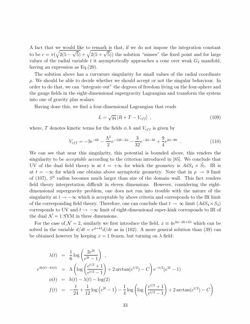
A fact that we would like to remark is that, if we do not impose the integration constant

to be c = π(√

2(5 −√

5) +√

2(5 +√

5)) the solution “misses” the fixed point and for large

values of the radial variable t it asymptotically approaches a cone over weak G2 manifold,

having an expression as Eq.(20).

The solution above has a curvature singularity for small values of the radial coordinate

ρ. We should be able to decide whether we should accept or not the singular behaviour. In

order to do that, we can “integrate out” the degrees of freedom living on the four-sphere and

the gauge fields in the eight-dimensional supergravity Lagrangian and transform the system

into one of gravity plus scalars.

Having done this, we find a four-dimensional Lagrangian that reads

L =√g4 [R + T − Veff ] , (109)

where, T denotes kinetic terms for the fields φ, h and Veff is given by

Veff = −3e−6h − Λ2

2e−12h−2φ − 3

32e−2φ−4h +

9

4e2φ−8h . (110)

We can see that near this singularity, this potential is bounded above, this renders the

singularity to be acceptable according to the criterion introduced in [85]. We conclude that

UV of the dual field theory is at t = +∞ for which the geometry is AdS4 × S7. IR is

at t = −∞ for which one obtains above asymptotic geometry. Note that in ρ → 0 limit

of (107), S4 radius becomes much larger than size of the domain–wall. This fact renders

field theory interpretation difficult in eleven dimensions. However, considering the eight-

dimensional supergravity problem, one does not run into trouble with the nature of the

singularity at t→ −∞ which is acceptable by above criteria and corresponds to the IR limit

of the corresponding field theory. Therefore, one can conclude that t→ ∞ limit (AdS4×S4)

corresponds to UV and t→ −∞ limit of eight-dimensional super-kink corresponds to IR of

the dual N = 1 SYM in three dimensions.

For the case of N = 2, similarly we first introduce the field, x ≡ 4e2φ−2h+2λ which can be

solved in the variable d/dt = eφ+4λd/dr as in (102). A more general solution than (39) can

be obtained however by keeping x = 1 frozen, but turning on λ field:

λ(t) =1

6log

(

2e2t

e2t − 1

)

,

e4h(t)−4λ(t) = Λ

(

log

(

et/2 + 1

et/2 − 1

)

+ 2 arctan(et/2) − C

)

e−t/2(e2t − 1)

φ(t) = h(t) − λ(t) − log(2)

f(t) = − t

24+

1

12log

(

e2t − 1)

− 1

4log

(

log

(

et/2 + 1

et/2 − 1

)

+ 2 arctan(et/2) − C

)

33

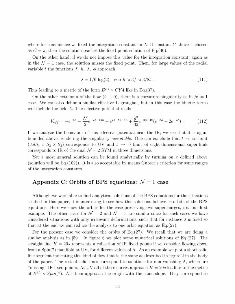
where for convinience we fixed the integration constant for λ. If constant C above is chosen

as C = π, then the solution reaches the fixed point solution of Eq.(46).

On the other hand, if we do not impose this value for the integration constant, again as

in the N = 1 case, the solution misses the fixed point. Then, for large values of the radial

variable t the functions f, h, λ, φ approach

λ = 1/6 log(2), φ ≈ h ≈ 3f ≈ 3/8t . (111)

Thus leading to a metric of the form E2,1 × CY 4 like in Eq.(37).

On the other extremun of the flow (t → 0), there is a curvature singularity as in N = 1

case. We can also define a similar effective Lagrangian, but in this case the kinetic terms

will include the field λ. The effective potential reads

Veff = −e−6h − Λ2

2e−2φ−12h + e2φ−8h−4λ +

g2

32e−2φ−4h(e−8λ − 2e−2λ) . (112)

If we analyze the behaviour of this effective potential near the IR, we see that it is again

bounded above, rendering the singularity acceptable. One can conclude that t → ∞ limit

(AdS4 × S2 × S2) corresponds to UV and t → 0 limit of eight-dimensional super-kink

corresponds to IR of the dual N = 2 SYM in three dimensions.

Yet a most general solution can be found analytically by turning on x defined above

(solution will be Eq.(102)). It is also acceptable by means Gubser’s criterion for some ranges

of the integration constants.

Appendix C: Orbits of BPS equations: N = 1 case

Although we were able to find analytical solutions of the BPS equations for the situations

studied in this paper, it is interesting to see how this solutions behave as orbits of the BPS

equations. Here we show the orbits for the case preserving two supercharges, i.e. our first

example. The other cases for N = 2 and N = 3 are similar since for such cases we have

considered situations with only irrelevant deformations, such that for instance λ is fixed so

that at the end we can reduce the analysis to one orbit equation as Eq.(27).

For the present case we consider the orbits of Eq.(27). We recall that we are doing a

similar analysis as in [59]. In figure 6 we plot some numerical solutions of Eq.(27). The

straight line H = 20s represents a collection of IR fixed points if we consider flowing down

from a Spin(7) manifold at UV, for different values of Λ. As an example we plot a short solid

line segment indicating this kind of flow that is the same as described in figure 2 in the body

of the paper. The rest of solid lines correspond to solutions for non-vanishing Λ, which are

“missing” IR fixed points. At UV all of these curves approach H = 20s leading to the metric

of E2,1 × Spin(7). All them approach the origin with the same slope. They correspond to

34

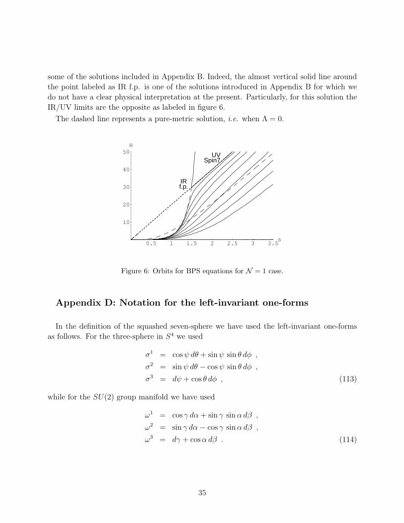
some of the solutions included in Appendix B. Indeed, the almost vertical solid line around

the point labeled as IR f.p. is one of the solutions introduced in Appendix B for which we

do not have a clear physical interpretation at the present. Particularly, for this solution the

IR/UV limits are the opposite as labeled in figure 6.

The dashed line represents a pure-metric solution, i.e. when Λ = 0.

0.5 1 1.5 2 2.5 3 3.5s

10

20

30

40

50H

UVSpin7

IRf.p.

Figure 6: Orbits for BPS equations for N = 1 case.

Appendix D: Notation for the left-invariant one-forms

In the definition of the squashed seven-sphere we have used the left-invariant one-forms

as follows. For the three-sphere in S4 we used

σ1 = cosψ dθ + sinψ sin θ dφ ,

σ2 = sinψ dθ − cosψ sin θ dφ ,

σ3 = dψ + cos θ dφ , (113)

while for the SU(2) group manifold we have used

ω1 = cos γ dα + sin γ sinα dβ ,

ω2 = sin γ dα− cos γ sinα dβ ,

ω3 = dγ + cosα dβ . (114)

35

References

[1] M. Atiyah, J. Maldacena and C. Vafa, “An M-theory flop as a large N duality,” J. Math.

Phys. 42, 3209 (2001) [arXiv:hep-th/0011256].

[2] M. Atiyah and E. Witten, “M-theory dynamics on a manifold of G(2) holonomy,”

arXiv:hep-th/0107177.

[3] S. Gukov and J. Sparks, “M-theory on Spin(7) manifolds. I,” arXiv:hep-th/0109025.

[4] B. S. Acharya, “Confining strings from G(2)-holonomy spacetimes,” arXiv:hep-

th/0101206.

[5] M. Cvetic, G. W. Gibbons, H. Lu and C. N. Pope, “Hyper-Kaehler Calabi metrics,

L**2 harmonic forms, resolved M2-branes, and AdS(4)/CFT(3) correspondence,” Nucl.

Phys. B 617, 151 (2001) [arXiv:hep-th/0102185].

[6] B. S. Acharya and C. Vafa, “On domain walls of N = 1 supersymmetric Yang-Mills in

four dimensions,” arXiv:hep-th/0103011.

[7] J. Gomis, “D-branes, holonomy and M-theory,” Nucl. Phys. B 606, 3 (2001) [arXiv:hep-

th/0103115].

[8] M. Cvetic, G. W. Gibbons, H. Lu and C. N. Pope, “New complete non-compact Spin(7)

manifolds,” Nucl. Phys. B 620, 29 (2002) [arXiv:hep-th/0103155].

[9] M. Cvetic, G. W. Gibbons, H. Lu and C. N. Pope, New Cohomogeneity One Metrics

With Spin(7) Holonomy math.DG/0105119

[10] J. D. Edelstein and C. Nunez, “D6 branes and M-theory geometrical transitions from

gauged supergravity,” JHEP 0104, 028 (2001) [arXiv:hep-th/0103167].

[11] A. Brandhuber, J. Gomis, S. S. Gubser and S. Gukov, “Gauge theory at large N and

new G(2) holonomy metrics,” Nucl. Phys. B 611, 179 (2001) [arXiv:hep-th/0106034].

[12] M. Cvetic, G. W. Gibbons, H. Lu and C. N. Pope, “Resolved branes and M-theory on

special holonomy spaces,” arXiv:hep-th/0106177.

[13] J. Gomis and T. Mateos, “D6 branes wrapping Kaehler four-cycles,” Phys. Lett. B 524,

170 (2002) [arXiv:hep-th/0108080].

[14] M. Cvetic, G. W. Gibbons, H. Lu and C. N. Pope, “Ricci-flat metrics, harmonic forms

and brane resolutions,” arXiv:hep-th/0012011.

[15] E. Witten, “Anomaly cancellation on G(2)manifolds,” arXiv:hep-th/0108165.

36

[16] M. Cvetic, G. W. Gibbons, H. Lu and C. N. Pope, “Cohomogeneity one manifolds of

Spin(7) and G(2) holonomy,” arXiv:hep-th/0108245.

[17] B. Acharya and E. Witten, “Chiral fermions from manifolds of G(2) holonomy,”

arXiv:hep-th/0109152.

[18] R. Blumenhagen and V. Braun, “Superconformal field theories for compact G(2) mani-

folds,” JHEP 0112, 006 (2001) [arXiv:hep-th/0110232]; R. Blumenhagen and V. Braun,

“Superconformal field theories for compact manifolds with Spin(7) holonomy,” JHEP

0112, 013 (2001) [arXiv:hep-th/0111048].

[19] J. Gomis, “On SUSY breaking and chiSB from string duals,” Nucl. Phys. B 624, 181

(2002) [arXiv:hep-th/0111060].

[20] G. Curio, B. Kors and D. Lust, “Fluxes and branes in type II vacua and M-theory

geometry with G(2) and Spin(7) holonomy,” arXiv:hep-th/0111165.

[21] M. Cvetic, G. Shiu and A. M. Uranga, “Chiral type II orientifold constructions as M

theory on G(2) holonomy spaces,” arXiv:hep-th/0111179.

[22] M. Cvetic, G. W. Gibbons, H. Lu and C. N. Pope, “M-theory conifolds,” arXiv:hep-

th/0112098.

[23] A. Brandhuber, “G(2) holonomy spaces from invariant three-forms,” arXiv:hep-

th/0112113.

[24] K. Sfetsos, “Integrable reductions of Spin(7) and G(2) invariant self-dual Yang-Mills

equations and gravity,” arXiv:hep-th/0112117.

[25] M. Cvetic, G. W. Gibbons, H. Lu and C. N. Pope, “A G(2) unification of the deformed

and resolved conifolds,” arXiv:hep-th/0112138.

[26] R. Hernandez and K. Sfetsos, “An eight-dimensional approach to G(2) manifolds,”

arXiv:hep-th/0202135.

[27] S. Gukov and D. Tong, “D-brane probes of G(2) holonomy manifolds,” arXiv:hep-

th/0202125.

[28] S. Gukov and D. Tong, “D-brane probes of special holonomy manifolds, and dynamics

of N = 1 three-dimensional gauge theories,” arXiv:hep-th/0202126.

[29] G. T. Horowitz and A. Strominger, “Black Strings And P-Branes,” Nucl. Phys. B 360,

197 (1991).

37

[30] T. Eguchi and A. J. Hanson, “Asymptotically Flat Selfdual Solutions To Euclidean

Gravity,” Phys. Lett. B 74, 249 (1978).

[31] R. Bryant and S. Salamon, “On the construction of some Complete Metrics with Ex-

ceptional Holonomy,” Duke Math. J. 58 (1989) 829. G. W. Gibbons, D. N. Page and

C. N. Pope, “Einstein Metrics On S**3 R**3 And R**4 Bundles,” Commun. Math.

Phys. 127, 529 (1990).

[32] E. Calabi, “Metriques kahleriennes et fibres holomorphes,” Ann. Scient. Ecole Norm.

Sup. 12, (1979) 269.

[33] R. Hernandez, “Branes wrapped on coassociative cycles,” Phys. Lett. B 521, 371 (2001)

[arXiv:hep-th/0106055].

[34] S. S. Gubser, “TASI lectures: Special holonomy in string theory and M-theory,”

arXiv:hep-th/0201114.

[35] A. Salam and E. Sezgin, “D = 8 Supergravity,” Nucl. Phys. B 258, 284 (1985).

[36] B. Acharya, X. de la Ossa and S. Gukov, “G-flux, Supersymmetry and Spin(7) mani-

folds,” arXiv:hep-th/0201227.

[37] D. Berenstein, J. Maldacena and H. Nastase, “Strings in flat space and pp waves from

N = 4 super Yang Mills,” arXiv:hep-th/0202021.

[38] R. R. Metsaev and A. A. Tseytlin, “Exactly solvable model of superstring in plane wave

Ramond-Ramond background,” arXiv:hep-th/0202109.

[39] M. Blau, J. Figueroa-O’Farrill and G. Papadopoulos, “Penrose limits, supergravity and

brane dynamics,” arXiv:hep-th/0202111.

[40] D. Berenstein, C. P. Herzog and I. R. Klebanov, “Baryon spectra and AdS/CFT corre-

spondence,” arXiv:hep-th/0202150.

[41] N. Itzhaki, I. R. Klebanov and S. Mukhi, “PP wave limit and enhanced supersymmetry

in gauge theories,” arXiv:hep-th/0202153.

[42] J. Gomis and H. Ooguri, “Penrose limit of N = 1 gauge theories,” arXiv:hep-th/0202157.

[43] J. G. Russo and A. A. Tseytlin, “On solvable models of type IIB superstring in NS-NS

and R-R plane wave backgrounds,” arXiv:hep-th/0202179.

[44] L. A. Zayas and J. Sonnenschein, “On Penrose limits and gauge theories,” arXiv:hep-

th/0202186.

38

[45] M. Hatsuda, K. Kamimura and M. Sakaguchi, “From super-AdS(5) x S**5 algebra to

super-pp-wave algebra,” arXiv:hep-th/0202190.

[46] M. Alishahiha and M. M. Sheikh-Jabbari, “The PP-wave limits of orbifolded AdS(5) x

S**5,” arXiv:hep-th/0203018.

[47] M. Billo’ and I. Pesando, “Boundary states for GS superstrings in an Hpp wave back-

ground,” arXiv:hep-th/0203028.

[48] N. w. Kim, A. Pankiewicz, S. J. Rey and S. Theisen, “Superstring on pp-wave orbifold

from large-N quiver gauge theory,” arXiv:hep-th/0203080.

[49] M. Cvetic, H. Lu and C. N. Pope, “Penrose Limits, PP-Waves and Deformed M2-

branes,” arXiv:hep-th/0203082.

[50] T. Takayanagi and S. Terashima, “Strings on orbifolded pp-waves,” arXiv:hep-

th/0203093.

[51] E. Floratos and A. Kehagias, “Penrose limits of orbifolds and orientifolds,” arXiv:hep-

th/0203134.

[52] M. Cvetic, H. Lu and C. N. Pope, “Gauged six-dimensional supergravity from massive

type IIA,” Phys. Rev. Lett. 83, 5226 (1999) [arXiv:hep-th/9906221].

[53] O. Pelc and R. Siebelink, “The D2-D6 system and a fibered AdS geometry,” Nucl. Phys.

B 558, 127 (1999) [arXiv:hep-th/9902045].

[54] K. A. Intriligator and N. Seiberg, “Mirror symmetry in three dimensional gauge theo-

ries,” Phys. Lett. B 387, 513 (1996) [arXiv:hep-th/9607207].

[55] J. de Boer, K. Hori, H. Ooguri and Y. Oz, “Mirror symmetry in three-dimensional gauge

theories, quivers and D-branes,” Nucl. Phys. B 493, 101 (1997) [arXiv:hep-th/9611063].

[56] M. Bershadsky, C. Vafa and V. Sadov, “D-Branes and Topological Field Theories,”

Nucl. Phys. B 463, 420 (1996) [arXiv:hep-th/9511222].

[57] J. Maldacena and C. Nunez, “Supergravity description of field theories on curved mani-

folds and a no go theorem,” Int. J. Mod. Phys. A 16, 822 (2001) [arXiv:hep-th/0007018].

[58] J. M. Maldacena and C. Nunez, “Towards the large N limit of pure N = 1 super

Yang-Mills,” Phys. Rev. Lett. 86 (2001) 588 [arXiv:hep-th/0008001].

[59] B. S. Acharya, J. P. Gauntlett and N. Kim, “Fivebranes wrapped on associative three-

cycles,” Phys. Rev. D 63, 106003 (2001) [arXiv:hep-th/0011190].

39

[60] H. Nieder and Y. Oz, “Supergravity and D-branes wrapping special Lagrangian cycles,”

JHEP 0103, 008 (2001) [arXiv:hep-th/0011288].

[61] J. P. Gauntlett, N. Kim and D. Waldram, “M-fivebranes wrapped on supersymmetric

cycles,” Phys. Rev. D 63, 126001 (2001) [arXiv:hep-th/0012195].

[62] C. Nunez, I. Y. Park, M. Schvellinger and T. A. Tran, “Supergravity duals of gauge

theories from F (4) gauged supergravity in six dimensions,” JHEP 0104, 025 (2001)

[arXiv:hep-th/0103080].

[63] M. Schvellinger and T. A. Tran, “Supergravity duals of gauge field theories from SU(2)

x U(1) gauged supergravity in five dimensions,” JHEP 0106, 025 (2001) [arXiv:hep-

th/0105019].

[64] J. P. Gauntlett, N. Kim, S. Pakis and D. Waldram, “Membranes wrapped on holomor-

phic curves,” Phys. Rev. D 65, 026003 (2002) [arXiv:hep-th/0105250].

[65] Y. Imamura, “1/4 BPS solutions in massive IIA supergravity,” Prog. Theor. Phys. 106,

653 (2001) [arXiv:hep-th/0105263].

[66] J. P. Gauntlett, N. Kim, D. Martelli and D. Waldram, “Wrapped fivebranes and N = 2

super Yang-Mills theory,” Phys. Rev. D 64, 106008 (2001) [arXiv:hep-th/0106117].

[67] J. P. Gauntlett and N. Kim, “M-fivebranes wrapped on supersymmetric cycles. II,”

arXiv:hep-th/0109039.

[68] T. A. Tran, “Gauged supergravities from spherical reductions,” arXiv:hep-th/0109092.

[69] J. Gomis and J. G. Russo, “D = 2+1 N = 2 Yang-Mills theory from wrapped branes,”

JHEP 0110, 028 (2001) [arXiv:hep-th/0109177].

[70] J. P. Gauntlett, N. w. Kim, D. Martelli and D. Waldram, “Fivebranes wrapped on SLAG

three-cycles and related geometry,” JHEP 0111, 018 (2001) [arXiv:hep-th/0110034].

[71] P. Di Vecchia, H. Enger, E. Imeroni and E. Lozano-Tellechea, “Gauge theories from

wrapped and fractional branes,” arXiv:hep-th/0112126.

[72] J. P. Gauntlett, N. Kim, S. Pakis and D. Waldram, “M-Theory solutions with AdS

factors,” arXiv:hep-th/0202184.

[73] H. J. Boonstra, K. Skenderis and P. K. Townsend, “The domain wall/QFT correspon-

dence,” JHEP 9901, 003 (1999) [arXiv:hep-th/9807137].

[74] L. Jarv and C. V. Johnson, “Orientifolds, M-theory, and the ABCD’s of the enhancon,”

Phys. Rev. D 62, 126010 (2000) [arXiv:hep-th/0002244].

40

[75] D. Joyce, Compact Manifolds With Special Holonomy, (Oxford University Press, 2000).

[76] M. B. Green, J. A. Harvey and G. W. Moore, “I-brane inflow and anomalous couplings

on D-branes,” Class. Quant. Grav. 14, 47 (1997) [arXiv:hep-th/9605033].

[77] M.J. Duff, H. Lu, C.N. Pope, E. Sezgin, “Supermembranes with fewer supersymme-

tries,” Phys. Lett. B 371, 206 (1996) [arXiv:hep-th/9511162].

[78] L. Castellani, A. Ceresole, D. D’Auria, S. Ferrara, P. Fre’, “G/H M-Branes and

AdS(p+2) geometries,” Nucl. Phys. B 527, 442 (1998) [arXiv:hep-th/9803039].

[79] M.J. Duff, B.E.W. Nilsson, C.N. Pope, “Squashed supersymmetry breaking by the

squashed seven sphere,” Phys. Rev. Lett. 50, 2043 (1983)

[80] D. S. Freed and E. Witten, “Anomalies in string theory with D-branes,” arXiv:hep-

th/9907189.

[81] E. Witten, “On flux quantization in M-theory and the effective action,” J. Geom. Phys.

22, 1 (1997) [arXiv:hep-th/9609122].

[82] I.R. Klebanov and E. Witten, “ADS/CFT correspondence and symmetry breaking,”

Nucl. Phys. B 556, 89 (1999) [arXiv:hep-th/9905104].

[83] C. Ahn and S. Rey, “Three dimensional CFT’s and RG flow from squashing M2-brane

horizon,” Nucl. Phys. B 565, 210 (2000) [arXiv:hep-th/9908110].

[84] M.J. Duff, B.E.W. Nilsson, C.N. Pope, “Kaluza-Klein supergravity,” Phys. Rept. 130,

1 (1986)

[85] S. S. Gubser, “Curvature singularities: The good, the bad, and the naked,” arXiv:hep-

th/0002160.

[86] P. Merlatti, “M-theory on AdS(4) x Q(111): The complete Osp(2|4) x SU(2) x SU(2)

x SU(2) spectrum from harmonic analysis,” Class. Quant. Grav. 18, 2797 (2001)

[arXiv:hep-th/0012159].

[87] D. Fabbri, P. Fre’, L. Gualtieri, C. Reina, A. Tomasiello, A. Zaffaroni and A. Zampa,

“3-D superconformal field theories from Sasakian seven manifolds: New nontrivial evi-

dences for AdS(4)/CFT(3),” Nucl. Phys. B 577, 547 (2000) [arXiv:hep-th/9907219];

[88] D. Fabbri, “Three dimensional conformal field theories from Sasakian seven-manifolds,”

arXiv:hep-th/0002255.

[89] G. Dall’Agata, “N = 2 conformal field theories from M2-branes at conifold singularities,”

Phys. Lett. B 460, 79 (1999) [arXiv:hep-th/9904198].

41

[90] C. h. Ahn, “N = 2 SCFT and M theory on AdS(4) x Q(1,1,1),” Phys. Lett. B 466, 171

(1999) [arXiv:hep-th/9908162].

[91] K. Oh and R. Tatar, “Three dimensional SCFT from M2 branes at conifold singulari-

ties,” JHEP 9902, 025 (1999) [arXiv:hep-th/9810244].

[92] D. Fabbri, P. Fre, L. Gualtieri and P. Termonia, “Osp(N|4) supermultiplets as conformal

superfields on d(AdS(4)) and the generic form of N = 2, D = 3 gauge theories,” Class.

Quant. Grav. 17, 55 (2000) [arXiv:hep-th/9905134].

[93] B. S. Acharya, J. M. Figueroa-O’Farrill, C. M. Hull and B. Spence, “Branes at conical

singularities and holography,” Adv. Theor. Math. Phys. 2, 1249 (1999) [arXiv:hep-

th/9808014].

[94] D. R. Morrison and M. R. Plesser, “Non-spherical horizons. I,” Adv. Theor. Math. Phys.

3, 1 (1999) [arXiv:hep-th/9810201].

[95] C. P. Herzog and I. R. Klebanov, “Gravity duals of fractional branes in various dimen-

sions,” Phys. Rev. D 63, 126005 (2001) [arXiv:hep-th/0101020].

[96] A. Kapustin and M. J. Strassler, “On mirror symmetry in three dimensional Abelian

gauge theories,” JHEP 9904, 021 (1999) [arXiv:hep-th/9902033].

[97] P. Termonia, “The complete N = 3 Kaluza-Klein spectrum of 11D supergravity on

AdS(4) x N(010),” Nucl. Phys. B 577, 341 (2000) [arXiv:hep-th/9909137].

[98] M. Billo, D. Fabbri, P. Fre, P. Merlatti and A. Zaffaroni, “Rings of short N = 3 su-

perfields in three dimensions and M-theory on AdS(4) x N(0,1,0),” Class. Quant. Grav.

18, 1269 (2001) [arXiv:hep-th/0005219].

[99] L. J. Romans, “The F(4) Gauged Supergravity In Six-Dimensions,” Nucl. Phys. B 269,

691 (1986).

[100] M. Petrini and A. Zaffaroni, “The holographic RG flow to conformal and non-conformal

theory,” arXiv:hep-th/0002172.

[101] V.L. Campos, G. Ferretti, H. Larsson, D. Martelli and B.E.W. Nilsson, “A study of

holographic RG flows in D = 6 and D = 3,” JHEP 0006, 023, (2000) [arXiv:hep-

th/0003151].

[102] D. Z. Freedman, S. S. Gubser, K. Pilch and N. P. Warner, “Renormalization group

flows from holography supersymmetry and a c-theorem,” Adv. Theor. Math. Phys. 3,

363 (1999) [arXiv:hep-th/9904017].

42

[103] D. Z. Freedman, S. S. Gubser, K. Pilch and N. P. Warner, “Continuous distributions of

D3-branes and gauged supergravity,” JHEP 0007, 038 (2000) [arXiv:hep-th/9906194].

[104] A. Loewy and Y. Oz, “Branes in Special Holonomy Backgrounds,” arXiv:hep-

th/0203092.

[105] E. Cremmer, B. Julia and J. Scherk, “Supergravity Theory In 11 Dimensions,” Phys.

Lett. B 76, 409 (1978).

43