RF ionization of the lower ionosphere

Radio Science, Volume 26, Number 5, Pages 1345-1360, September-October 1991

RF ionization of the lower ionosphere

K. Tsang, K. Papadopoulos ,1 A. Drobot, and P. Vitello

Science Applications International Corporation, McLean, VIrginia

T. Wallace and R. Shanny

ARCO Power Technologies Incorporated, Washington, D. C.

(Received June 4, 1990; revised February 8, 1991; accepted February 8, 1991.)

A comprehensive analysis of the ionization rates of air by RF fields is presented. The analysis relies on a time-dependent code which treats the electron energization with a Fokker-Planck type model and the inelastic energy losses with a multiple time scale technique. Derivation of ionization rates for parameters of interest To D region ionospheric by ground-based RF transmitters with frequency much higher than the electron neutral collision frequency is emphasized. The study provides a physical understanding of the ionization proces and its associated efficiency by combining the computational results with analytic theory. It is shown that for values of quiver energies E « I, where I is the ionization potential, the electron production time corresponds to the electron energization time from energies below 2 eV to 20-25 eV. The analytic expressions derived are consistent with the computational results over 6 orders of magnitude in ionization rates and over 2 orders of magnitude in values of E. Power threshold definitions are clarified, and the pitfalls of using fluid descriptions or effective electric field notions are discussed The paper concludes with an assessment the power requirements for ionization at 70-km ionospheric altitude with RF in the 100-900 MHz frequency range.

1. IN1RODUCTION

High power RF breakdown of neutral gases is a com­mon laboratory plasma production technique. The potential for enhancing the ionization of the middle atmosphere and the lower ionosphere by using similar techniques was recognized as early as 1937. Bailey [1937, 1938] suggested that injection of RF power in the ionosphere from ground-based transmitters operating in the 1.3 - 1.4 MHz frequency range can increase the plasma density of the ionospheric D region to the extent

1 Also at ARCO Power Technologies Incorporated, Wash­ington, D. C. and Department of Physics and Astronomy, Uni­versity of Maryland, College Park.

Copyright 1991 by the American Geophysical Union.

Paper number 91RSOO580. 0048-6604/91/91RS-00580$08.00

1345

that it can retlect RF frequencies. The particular frequency range was chosen because it coincides wi!h the electron gy­rofrequency no in the Earth's magnetic field, thereby enhanc­ing !he coupling of !he RF energy to !he plasma. It was soon recognized that at such a low frequency the RF wave suffers strong self absorption prior to reaching the breakdown region and the resulting ionization level is exttemely low [Clavier, 1961; Gurevich, 1965]. Furthermore, the increase in the value of the elastic electron neutral collision rate /I resulting from the local heating would produce quickly a situation where /I

> no and !hus eliminate the advantages of heating at !he cy­clotron frequency. Lombardini [1965] suggested !hat use of higher frequency (50 MHz) can reduce !he severity of the self absorption problem so !hat useful levels of ionization can be produced. The models of RF absorption and electron energiza­tion used by Lombardini were very crude, resulting in major uncertainties in !he power density required for the creation of a useful plasma density. More refined models were developed

1346 TSANG ET AL.: RF IONlZATION OF THE LOWER IONOSHPERE

later in the USSR [Gurevich, 1972, 1978; Borisov et aI., 1986] for VHF-UHF frequencies, using a kinetic description of the electron energization process. Most of the work utilized an­alytic approximations which give valid results only when the details of the resonant structure of the inelastic processes as­sociated with the molecular composition of the ambient gas are not critical. The most comprehensive analysis of the air breakdown problem was given by Kroll and Watson [1972] in a paper remarkable for its physical insight. The particu­lar study emphasized parameters relevant to high-density (i.e., in the range of standard atmospheric pressure) breakdown by lasers pulses. Although important scaling laws applicable to upper atmospheric and ionospheric densities are present, it is rather difficult to exlrapolate the results to the range of in­terest here. Furthermore, the computations were restricted to steady state solutions, ignored molecular dissociation, and em­phasized ionization near the breakdown threshold

The purpose of this paper is to present a comprehensive local analysis of the physics of ionization of the ionospheric D region caused by injection of RF waves from ground-based lransmitters. The analysis relies on a kinetic description of the electron energization by RF waves given by the solution of a time-dependent Foller-Planck (FP) code. The inelastic interaction of the electrons with the molecular gas is treated in the code by a multiple time scale technique. The details of the numerical scheme can be found in Short et aI. [1990]. An important ingredient of the study is the use of the most up-to-date set of cross sections. The output of the study is a comprehensive model of the local ionization rate as a function of the RF frequency and local power density, and the neulral gas density and constitution. The study provides the necessary input to realistic multidimensional models of D region ionization which include self absorption of the RF fields coupled to the dynamic increase of the plasma density and energy. The latter study is in progress and its results will be reported in a future publication.

In the following sections, we discuss the RF ionization process in detail. The basic physics of the electron energiza­tion by RF waves and the resultant ionization in the iono­spheric D region are treated in section 2. The discussion in­cludes elucidation of the energy dependence of the dominant elastic and inelastic processes in the molecular ionospheric gas, resultant regions of self-similar solutions and a quali­tative analysis of the physics of particle soun:es and losses. Important dimensionless parameters are also introduced. Nu­merical solutions of the time-dependent FP equation for the high-frequency regime, w i! 11m, where w is the RF frequency and v'" the maximum value of the elastic electron-neulral col­lision frequency, are presented in sections 3 and 4. The re­sults include universal curves of the ionization and attachment rates versus RF power density and frequency and an analysis of the stationary value of the electron distribution function. In section 5 the numerical results are compared with an ana­lytic model of the ionization rate and efficiency versus power density and frequency. The ionization physics in the low­frequency regime w < v'" is briefly discussed in section 6.

Practical results concerning the power and frequency require­ments for ionization in the ionospheric D region form the sub­ject of section 7. The last section summarizes the essential points and the key formulae derived in the paper.

2. BASIC CONCEPTS

The interaction of a weakly ionized plasma under iono­spheric D region conditions with RF waves results in modifi­cation of the electron distribution function F(£) described by an equation of the type [Zel'dovich and Raizer, 1965; Kroll and Watson, 1972; Gurevich, 1978; Hays et al., 1987]:

~F(£) = ..!..~£3/2D(£ w f)aF(£) - L(£) (la) at .,fi 8£ "at:

In (la), F(£) is normalized to the total electron density n(t) as 00 f d£..jiF(£, t) = net) (lb)

o

The diffusion coefficient D(£) is given by

D() 2_ v(£) £ = 3"£ 1 + v 2(£)/W2 (2)

where l is the quiver energy of an electron in the electric field of an RF wave of frequency w and peaIc amplitude Eo given by

(3)

v(£) is the collision frequency for momentum lransfer and L(£) is an operator that describes the relevant inelastic processes. For the ionospheric case under consideration here the operator L(£) includes rotational, vibrational, and electronic excitation processes as well as ionization and dissociative attachment (i.e., Oz + e - 0 + 0-) for the mixture of 80% N2 and 20% ~. The form of L(£) used in the computations and the range of its validity are discussed In deriving (la) we ignored lransport and assumed that the electron distribution is isotropic. These assumptions are easily justified for interactions in the 50-80 km altitude of interest here. It is, furthermore, assumed that hw « l < £. In comparing our solutions with Kroll and Watson [1972] as well as other papers dealing with the solution of the Boltzmann equation we should note that, as discussed in section 4, their normalization of the distribution function is different than (lb). Furthermore, the FP collision integral is equivalent to the Boltzmann collision integral in the limit of small; / £. The bulk of the paper deals with numerical solutions of (la) for various RF frequencies, power densities, and altitudes. It is, however, instructive to discuss first the basic physics concepts related to (la), which illuminate the understanding of the numerical results, the underlying scaling laws, and the generalization to other situations.

The first term of (la ) represents the collisional electron eneJgization rate. It can be decomposed into two terms. The first is the rate at which the average particle energy <t:> increases and is given by

TSANG ET AL.: RF IONIZATION OF THE LOWER IONOSHPERE 1347

(4)

The second represents the rate of increase of the avemge quadratic energy scattering and is given by

8 2 8t[< £2> - < £ >]:=< ~£2 >= £D(£). (5)

The diffusion coefficient 0(£) has a particularly simple fonn in the following limits. First, for eneJgies £ such that 11(£) «w,

(6)

In this energy range the rate of average energy increase is given ~by

(7)

Notice that since 11(£) ..... £11 with Q' = 1 - 0.5 up to about 20 e V, the electron energization is of the runaway type. The value of II saturates in the 20-30 eV range and has a maximum value given by

c o

N o

o

o o

~­::ll:, ..c~ .;:: ....... UJN

·-1 00

C 0.., ~I

u~ (])

W ... 1 o

on 1

..

o ....

10 I o

...

11m = 3 X 10-7 N sec-I (8)

a :: r :":: ~; r"~; :' : -:'::~ .::': . '.:~' ': : :-, ; .. ,"~"'. .' ~

......... :.' .:-:-; -,: .:-:

~ .. "=,":': .. ~': r:-:"': :'~ :',"~ ;:,:;: :':X(:':,": ,': ::' : :':'~T: ~'. !::; . . -:. : ......... :. .. '" ,-

"';': ~(·.~~:·:;-~~~·~~r:~·:: ':.:' ~:': :::;,-...

.... . : . .

:: :: 1 '~.~(:: :T~' ~. ". f ~ :r~r·:·1

where N is the neutral particle density per cm3• Second, for eneJgies such that w ~ 11(£), D( £) is weakly dependent on energy and the average energy increases linearly with time. Finally, for energies such that w « 11(£) the energization rate is independent of the RF frequency and the average energy increases as jlfJ - ,If}.. In the latter case the RF energization is analogous to energization by a DC electric field [McDonald, 1966]. As noted, (4) describes the average rate of energi.za­tion, while (5) describes the average energy variation about it which is representative of the formation of a high-energy tail. Notice that in the absence of losses, (la) has self-similar solutions with respect to time, which in the limits w » 11(£) and w « 11(£) correspond to runaway and Dryvestein electron distribution functions [Gurevich, 1978]. It is obvious that if processes requiring large Bnxes of energetic electrons, such as ionization processes, are of interest, it is advantageous to utilize the high-frequency regime. Furthermore, since in the high-frequency regime the energization rate is proportional to the quiver energy {", high frequencies require higher RF power

densities than low frequencies (i. e., 5 = const.) to achieve the same energization rate and result in an energetically inef­ficient process.

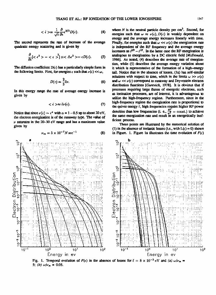
These points are illustrated by the numerical solution of (1) in the absence of inelastic losses (i.e., with L(£) = 0) shown in Figure. 1. Figure la illustrates the time evolution of F(£)

N o

o

o o

c o

:.;:;.-::Jl:, ..c~ .;:: ....... .~';' 00

c 0.., ~I

....... 0 u~ Q)

W ... I o

10 I o

b -, -, .... . .. .

:': .. ; ..... ; .. :;: . .. .... : .. '. . ~ ..

'. . : r :'~':'r:~::' . "::: .. : ::;' .' ' ...... . ..

".

1: .:.:' ~ :';'(\.:: :':'!: ~ :;~ :Tn'~r~~n:;' , •• ,., •• J •••••

... '.:.: ....

.. ~ ':::: . ·::·~·:T:T~r::;·

~. . . . . .. ~"" ...... . . ..

10-' 100 102 10-' 100 10' 102

Energy in ev Energy in ev Fig. 1. Temporal evolution of F(£) in the absence of losses for {" = 8 X 10-3 eV and (a) wIll", = 5; (b) wIll", = 0.05.

1348 TSANG ET AL.: RF IONIZATION OF THE LOWER IONOSHPERE

for quiver energy l = O.OOS eV and RF frequency w/v", = 5. The time evolution is presented in units of v.;l. Notice the flat runaway character of F(f) from low energies up to 20 eV at which point V(f) reaches its maximum value. From that point on, F(f) has a Maxwellian character as expected from (1) for V(f) and D(t") independent of energy. Since there are no energy losses, the characteristic temperature of the Maxwellian part increases with time. The runaway and the Maxwellian part of F(f) join smoothly near f :::::I 20 eV. For w < v'" the energy at which the runaway and the Maxwellian part join is lower than 20 eV and coincides with the value of f where V(f) :::::I w. One more featw'e of the energy dependence of F is obvious. The ftabless of F(f) is much larger in the region below 3 e V than above. The reason for this is that for f < 3 eV v "" f, while the dependence of v on energy becomes progressively weaker at higher energies. Figure 1 b shows the evolution of F(f) for L(f) = 0 at the same quiver energy (l"" 0.008 eV), but w « V m• It is clear that below 2 eV, F(f) has retained its runaway character; however, it falls much faster than Maxwellian for energies above 2 eV. In that range the solution is of the Dryvestein type since for 2 eV < f < 20 eV, D(f) "" l/fO: with Q' positive. Again, the joining of the two types of distributions is near the energy f at which w = V(f). This analysis allows us 10 characterize the energization process as described by:

~ I o

~ ,..-...1 N 0 E~

u

N O~

1 ~o o~

'+-

C/l C 0" ~-u l

Q)~ CI1

C/l C/l 0", ~~

UI o

~ 1 o

a

. .. d.:::. ~': . ... ' .. , . ',"., ~ , ... . , ... , ,,)

. ...................... ...... '." ... . . . ;: ':':.::. ~ ';.:.: l' : . : .. ; .: ..... ~. ~ ~ -:': ; : ........... :.: ..... : ......... ', .: ... : .. :.:.; ....... , .. .. .. .. . .... .

....... . .. : ... ;~~~~. ~r~n~~~r .... ; ... ;.:. ;,;.' ; ........... : .... : .... : :. ;.:: . . : . : . :'.: . ~ ; ~ . . ... -. .. . .. .. ... -. -~ ..... :

. .. i . .

.. . .. ... .

:'~':'~ ~~::: :'::~:':~:: .·~·r·~: ~: :':'~ ~·~·:cii~J.~~~~: >.;~.~. ~ ~'~('; :':~::~; .. .. .. ' ..... ,. ." . . , ....... '. .. . ...:.:::.: ::-;'::.:

............ ;

... :~ .. , .. :.::.: ... : ... :::!

:::::<:.:::.::::::

~~)~l~\ ':': ·::;.\F: .

. . . , . ~ : ~ ~.::. :\\ .

1. For w « v", most of the RF energy is deposited as a bulk: heating. F(f) is flat topped, and high-energy elec­trons are suppressed. Since efficient ionization requires large fluxes of suprathermal electrons, the range w « Vm should be avoided. Notice that, if the presence of a drift in the distribu­tion function can be ignored, the w « Vm regime is analogous to energization by a DC electric field.

2. The production of suprathermal electrons is optimized in the w ~ Vm range. In fact, since l "" P / w2 , the optimum value of w, from the power density P point of view, is near w ~ Vm • We will return 10 this pointiater on.

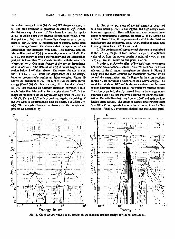
In order 10 explore the effect of inelastic losses we present first their cross-section stuClure. The cross sections for losses relevant 10 the D region ionosphere are shown in Figure 2 along with the cross sections for momentum transfer which control the energization rate. In Figure 2a the cross sections for the N2 are shown as a function of the electton energy. The solid line at about 1OIscm2 is the momentum transfer cross section between electrons and N2 10 which we referred earlier. The closely packed, sharply peaked lines in the energy range between 1 and 3 eV are the cross sections for vibrational exci­tation. The solid line that rises from "" 15e V and up is the ion­ization cross section. The group of dashed lines ranging from 5 10 100 eV corresponds 10 excitation cross sections for line emission. Finally, a prominent dashed line that almost paral-

N

z~ 1

~o o~

'+-

C/l C 0" :;::;-u l

Q)~ CI1

C/l C/l

e~ Ul:,

~ 1 o

b

100 101 102 10-1 100

Energy In ev Energy In ev Fig. 2. Cross-section values as a function of the incident electton energy for (a) N2 and (b) Oa.

TSANG ET AL.: RF IONIZATION OF THE LOWER IONOSHPERE 1349

leIs the ionization cross section is the dissociation cross section for Nz. In Figure 2b similar cross sections are shown for Oz. These cross sections are, in general, lower than those of Nz, and the ionization threshold (~ 12 eV) is slightly lower. Since the number density of Oz is only a small fraction of the Nz density (about 20%), the role of the Oz inelastic cross sections is minimal, with one notable exception. The exception is the cross section which represents electron loss due to dissociative attachment (Oz + e -+ 0- + 0) (Figure 2b). It occurs near 6.7 eV and has a strong resonant character. There is no analogous process, for Nz since Nz is not an electronegative gas. In the absence of transport processes attachment represents the only electron loss from the system and thus determines the value of the minimum power required for net electron production. An additional particle loss process is due to three body auach­mentof02(02 + 02 + e-+ 02 +02). In thcrangeofneutral densities of interest here the dissociative attachment, being a two-body process, dominates over the three-body attachment, at least during breakdown.

In energizing electrons from below 1 eV to ionization en­ergy the first prominent loss is due to the vibrational excitation of Nz (Figure 2a) by electron collisions. It occurs near 2.6 eV, and the overall energy loss due to Nz vibrational excitation can be approximated by [Kroll and Watson, 1972]:

Lv(t") = 8.6 X 1O-2vmV£ X exp[-4(€-2.6)2]eV/sec (9)

where the energy € is in units of electron volts. On the other hand, the cnergization rate near 2.6 eV as given by (6) is

i. ~ fv(2.6eV) (10)

From (9) and (10) we find that the quiver energy required to overcome the vibrational barrier completely

(11)

In the absence of the quadratic energy scattering term given by (5), power densities below the ones given by (11) cannot accelerate any electrons to ionization energies. The energization described by (5) is diffusive and allows electrons to reach ionization energies even in the presence of large losses or equivalently for power densities much lower than fl. The electron motion along the energy axis is made up of random energy jumps of finite magnitude and has a stochastic character. As a result a fraction of the electron flux has a finite probability to accelerate past the 3-eV barrier and thus form a high-energy tail. Notice that (1) is similar to the Schrondinger equation [Landau and Li/shitz, 1985; Gurevich, 1978] which describes the penetration of particles through a potential barrier. For (1) the barrier is due to energy loss by inelastic collisions.

The above comments are graphically illustrated by ex­amining the time evolution of F(€) using the numerical code

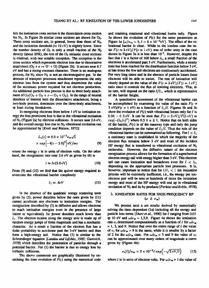
and retaining rotational and vibrational losses only. Figure 3a shows the evolution of F(€) for the same parameters as Figure Ia (wlvm = 5, f = 8 x 1O-3eV). The effect of the vi­brational barrier is clear. While in the lossless case the ra­tio F( € ~ 3 e V)/ F( € ~ 1 e V) was of order unity in the case shown in Figure 3a it is less than 10-5• However, despite the fact that f is a factor of 100 below flo a small fraction of the electrons is accelerated past 3 eV. Furthermore, while a steady state has been reached for the distribution function below 3 eV, at late times the few tail electrons are continuously accelerated. For very long times and in the absence of particle losses these electrons will be able to ionize. The rate of ionization will clearly depend on the value of the F(€ = 3 eV)1 F(€ = 1 eV) ratio since it controls the flux of ionizing electrons. This, in its tum, will depend on the ratio i/flo which is representative of the barrier height.

A quantitative assessment of the vibrational barrier can be accomplished by examining the value of the ratio F(€ = 3 eV)IF(€ = 1 eV) as a function of fI/f. Figures 3b and 3c show the evolution of F(€) with vibrational losses only for f ~ 0.04 - 0.2 eV. It can be seen that F(€ = 3 eV)1 F(1 eV) ~ exp[-(fI/€t1 where 0.5 S as 1. Notice that on both sides of the barrier, F(€) is of the runaway type and only the jump condition depends on the value of iI/f. Thus the role of the vibrational barrier can be summarized as following. For f < f I a stationary state is established in which the majority of the electron flux remains below 3 eV and most of the incident HF energy flux is transferred to vibrational excitation of Nz molecules. However, the diffusive nature of the electron energization process allows for the formation of a suprathermal electron energy tail with energy higher than 3 eV. This electron tail can cause ionization and breakdown even for i < fl, depending on the appropriate particle loss processes. It is, however, important to notice that for f/fl < 1 the ionization process will be extremely inefficient, i.e., the energy per ion­electron pair will be tens or hundreds of times the ionization energy and most of the HF energy will end up in vibrational excitation of Nz and its by products [Perkins and Roble, 1978].

3. IONIZATION RAmS FOR HIGH-FREQUENCY RF (w ~ v",)

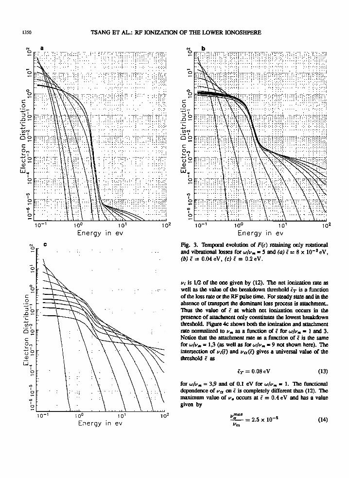
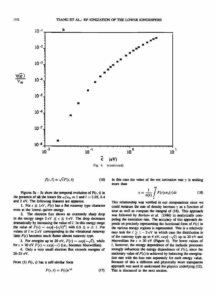
We present next a set results derived by numerically solving the time--<lependent (Ia) including all the energy and particle loss terms [Short et m., 1990] for l ranging from 0.Q1 tp 10 eV and wlv", = 1,3,9. Figure 4a shows the ionization rate Vi determined computationally as a function of f for wlv", = 1,3, and 9. Notice that over the entire range of f the value of Vi for wlv", = 9 is the same, while it is smaller by a factor of 2 for the wlv", case. For wlv", = 3 and 9 the value of Vi

can be approximated over many orders of magnitude a curve given by (Figure 4b):

vi(l)lvm = 3 x 10-2£ ezp( -";2 eV Ii) (12)

where f is in units of electron volts. For wlv", = 1 the value of

1350

N o

o

0 0

C 0

:.;:;-:;ll

..o~

.i: -+oJ en N

.-1

O~ C 0.., ~I

-+oJ 0 ()~ Q)

W..,. 1 0

It> 1 0

\0 1 0

N 0

0

0 0

c 0 ~ .... :::JI

..o~

.;:

..... en N .- 1 00

C 0.., '-I

..... 0 u~ Q)

w. 1 0

It> 1 0

'" 1 0

a .. . .. ~. ..

.. .....

..

10-1

C

10-1

TSANG ET AL.: RF IONIZATION OF THE LOWER IONOSHPERE

100 101

Energy In ev

10°

Energy In ev

c 0.., ~I

u~ Q)

W..,. 1 o

It> 1 o

\0 1 •• o

. ,', : ',': ~ ; .

10°

;- .. :-:.:-:-:-:,:

':::':'~:: r:;;':-:'; r~ !':':':::'~'r:'! :'f i':::;~; ,'. ~ :':':'" . .. . ... ', : ~.::.,:.;

=:: !'::~'~':~:l ~ :'~'~'!: n:, :':'; (nt::'::' .. : .. ;.; .... : .. ::. ::::.::':'::-.,:. .. : :' "': . ..:. : .:. : " : : . ~ : :. ::; ..• ,". . . . . . . . ", t.: ~.: :

Energy in ev

Fig. 3. Temporal evolution of F(f) retaining only rotational and vibrational losses for wIll". = 5 and (a) l = 8 x 1O-3 eV, (b) l = 0.04 eV, (c) l = 0.2 eV.

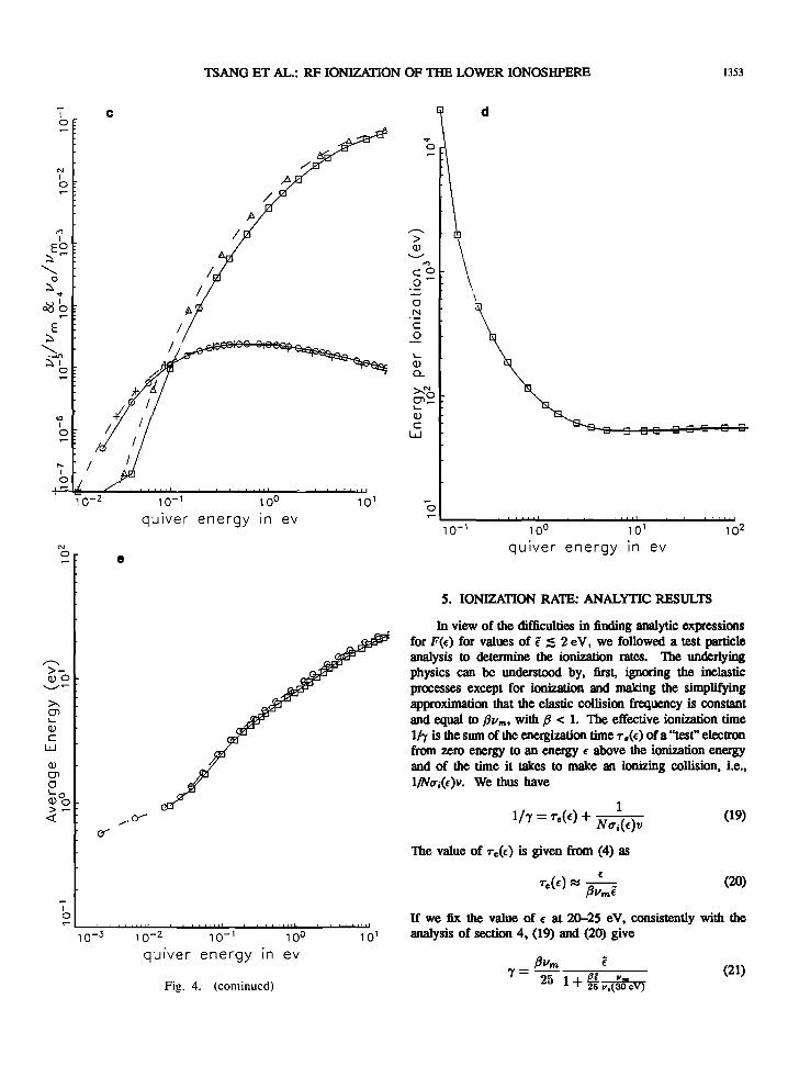
II; is 1/2 of the one given by (12). The net ionization rate as well as the value of the breakdown threshold IT is a function of the loss rate or the RF pulse time. For steady state and in the absence of transport the dominant loss process is attachment .. Thus the value of l at which net ionization occurs in the presence of attachment only constitutes the lowest breakdown threshold. Figure 4c shows both the ionization and attachment rate normalized to II '" as a function of l for wIll", = 1 and 3. Notice that the attachment rate as a function of l is the same for wIll", = 1,3 (as well as for wIll", = 9 not shown here). The intersection of 1I;(l) and 1I0(l) gives a universal value of the threshold l as

IT = 0.08eV (13)

for wIll", = 3,9 and of 0.1 eV for wIll", = 1. The functional dependence of 110 on l is completely different than (12). The maximum value of II. occurs at l = 0.4 eV and has a value given by

IIml .. ' _a_ = 2.5 X 10-5 (14)

11m

TSANG ET AL.: RF IONIZATION OF THE LOWER IONOSHPERE 1351

10.1 r ___ 8;;.... ________________ --,

10-2

10-3 ,

... 0 • ... . • 0. • o • ... • • 0. .. . .,.

•• • •

0·. • 10-4

10-5

10-7 •

• •

• .. • •

o· • o •

• • • • •

• o • • ... . •••

• .1!l.. = 1 Vm

• ...m.. = 3 vm o .JIl. = 9

Vm

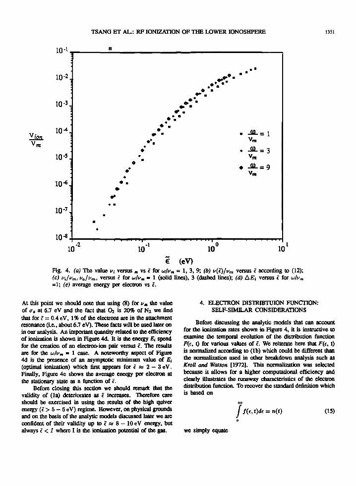
€ (eV) Fig. 4. (a) The value IIi versus '" vs l for wIll", = I, 3, 9; (b) 1I(f)/lIm versus l according to (12); (c) IIi/lim, lIa /lIm , versus l for wIll", = 1 (solid lines), 3 (dashed lines); (d) b.E; versus f for wIll", =1; (e) average energy per electron vs l.

At this point we should note that using (8) for 11", the value of (J'II at 6.7 eV and the fact that ~ is 20% of Nz we find that for l = 0.4 e V, 1 % of the electrons are in the attachment resonance (i.e., about 6.7 eV). These facts will be used later on in our analysis. An important quantity related to the efficiency of ionization is shown in Figure 4d. It is the eneIgy Ei spend for the creation of an electron-ion pair versus c. The results are for the wIll", = 1 case. A noteworthy aspect of Figure 4d is the presence of an asymptotic minimum value of Ei (optimal ionization) which first appears for l Il::: 2 - 3 eV. Finally, Figure 4e shows the average eneIgy per electron at the stationary state as a function of l.

Before closing this section we should reJJl8lk that the validity of (la) deteriorates as c increases. Therefore care should be exercised in using the results of the high quiver eneIgy (c > 5 - 6 eV) regime. However, on physical grounds and on the basis of the analytic models discussed later we are confident of their validity up to Cll::: 8 - 10 eV eneIgy, but always C < I where I is the ionization potential of the gas.

4. ELEC1RON DISTRIBTUION FUNCTION: SELF-SIMILAR CONSIDERATIONS

Before discussing the analytic models that can account for the ionization rates shown in Figure 4, it is instructive to examine the temporal evolution of the distribution function F(c, t) for various values of c. We reiterate here that F(c, t) is normalized according to (lb) which could be different than the nonnalization used in other breakdown analysis such as Kroll and Watson [1972]. This normalization was selected because it allows for a higher computational efficiency and clearly illustrates the runaway characteristics of the electron distnbution function. To recover the standard definition which is based on

00 f f(c, t)dc = n(t) (IS)

o

we simply equate

1352 TSANG ET AL.: RF IONIZATION OF THE LOWER IONOSHPERE

10 ·1 b

10 -2.

10 -3.

.. \({€) .. Vm

10-4 It

.. 10-5

It

10-6 .. 10 -7 ~

It 10-8

10 -2 10 ·1

€ Fig. 4.

f(f, t) = y'(F(f, t) (16)

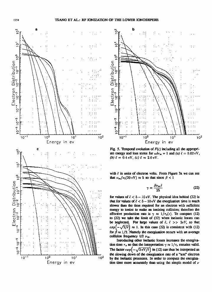
Figmes 5a - 5c show the temporal evolution of F(f, t) in the presence of all the losses for w/vm ~ 1 and l = 0.02, 0.4 and 2 eV. The following fealW"eS are apparent

1. For f ;S leV, F(f) has a flat runaway type character even at the lowest quiver energy.

2. The electron flux shows an extremely sharp drop in the energy range 2 e V ;S f ;S 4 e V. The drop decreases dramatically by increasing the value of l. In this energy range the value of F(f) '" exp[-(l/l)Q] with 0.5 ;S Q ;S 1. For values of l ~ 2 e V corresponding to the vibrational runaway limit F(f) becomes much flatter almost runaway type.

3. For energies up to 20 eV, F(f) '" exp(-.,fi), while for f > 20 eV F(f) '" exp( -f) (i.e., becomes Maxwellian).

4. Only a very small electron flux exceeds energies of 20-25 eV.

From (1) F(f, t) has a self-similar form

F(f,t) = F(f)e'Yt (17)

MM MM

M

M MM

M M

M M

.. .. ..

I~O 101

(eV) (continued)

In !his case the value of !he net ionization rate 'Y is nothing more than

00

'Y = n~t) J F(f)flTi(f)df (18)

o

This relationship was verified in our computations since we could measure !he rate of density increase 'Y as a function of time as well as compute the integral of (18). This approach was followed by Borisov et aI. [1986] in analytically com­puting the ionization rate. The accuracy of this approach de­pends on precisely representing the functional form of F(f) in the various energy regions is represented. This is a relatively easy task for l ~ 1 - 2 e V in which case the distribution is of !he runaway type up to 4 eV, exp( -.,fi) up to 20 eV and Maxwellian for f > 20 eV (Figure 6). For lower values of l, however, the energy dependence of the inelastic processes strongly influences the energy dependence of F(f), since the stationary value of F(f) is achieved by balancing the energiza­tion rate with the loss rate separately for each energy value. Because of this a d.i1Ierent and physically more transparent approach was used to understand the physics underlying (12). This is discussed in !he next section.

I 0

N 1 0

I'l 1

EO ~~

"'-0 ~ ... ~b

E ~

"'-. ...." ;::"1

0

'" 1 0

.... / 1

~i

N 0

~

>­Q)O '-"~

>-0' I.... Q) C

W

Q)

0' o 1....0 Q)O >~ «

1 o

10-2

c

e

TSANG ET AL.: RF IONIZATION OF THE WWER IONOSHPERE 1353

.A

/ .A

/

/

10-' 100

qUiver energy in ev

10-2 10- 1 100

qUiver energy In ev

Fig. 4. (continued)

d

~ In > \ Q)

\ "--"

'" CO o~

0 \ N

C 0

I.... Q) Q.

>-N ~~ I.... Q) C

W

o

100 10'

qUiver energy in ev

5. IONIZATION RA1E: ANALYTIC RESULTS

In view of the difficulties in finding analytic expressions for F(f.) for values of l =s 2 eV, we followed a test particle analysis to determine the ionization rates. The underlying physics can be understood by, first., ignoring the inelastic processes except for ionization and making the simplifying approximation that the elastic collision frequency is constant and equal to f3vm, with f3 < 1. The effective ionization time l/-y is the sum of the energization time T .«(.) of a "test" electron from zero energy to an energy f. above the ionization energy and of the time it takes to make an ionizing collision, i.e., l/Nui(f.)v. We thus have

1 l!r = T.(f.) + N ()

Ui (. V

The value of T,,(t:) is given from (4) as

(19)

(20)

If we fix the value of f. at 20-25 eV, consistently with the analysis of section 4, (19) and (20) give

f3vm l 1=- IH..

25 1 + 2~ JI,(;8'eV) (21)

1354

N o

o

o o

I... .... .~';' 00

c 0..., 1...1

.... 0 u~ Q.l

W ...

c o

I... ....

1 o

I()

1 o

'" 1 o

N o

o

. ~';' 00

c 0..., 1...1

.... 0 u~ Q.l

W ... 1 o

I()

1 o

'" 1 o

a

c

TSANG ET AL.: RF IONIZATION OF THE LOWER IONOSHPERE

,. "! , "',

100 101

Energy In ev

100 101

Energy In ev

c o

N o

o

o o

~­:;,1 ..c;! ·c .... .~';' 00

c 0.., '-I ..... 0 .. u~ Q.l

W ... 1 o

I()

1

b

o ..... . ..

'" 1 o

'., . .. .. ...

10°

Energy In ev

Fig. 5. Thmporal evolution of F(f) including all the appropri­ate energy and loss terms for w/v", = 1 and (a) f = 0.02 eV, (b) l = 0.4 eV, (c) l = 2.0 eV.

with l in units of electron volts. From Figme 3a we can see that vm /vi(20 eV) R:I 5 so that since (J < 1

(JVmf 1'=2s- (22)

for values of l < 5 - 10 e V. The physical idea behind (22) is that for values of l < 5 - 10 e V the energization time is much slower than the time required for an electron with sufficient energy to ionize to make an ionizing collision; therefore the effective production rate is l' R:I l/r.( f). To compare (12) to (22) we take the limit of (12) when inelastic losses can be neglected. For large values of l, l » 2eV, so that ezp( -..,f2fi) R:I 1. In this case (22) is consistent with (12)

for (J R:I 1/2. Namely the energization occurs with an average collision frequency Ifl v"'.

Introducing other inelastic losses increases the energiza­tion time r. so that the interpretation l' R:I l/r. remains valid.

The factorezp( -V2eV /l) in (12) can thus be interpreted as the slowing down of the energization rate of a "test" electron by the inelastic processes. In order to compute the energiza­tion time more accurately than using the simple model of v

TSANG ET AL.: RF IONlZATION OF THE WWER IONOSHPERE 1355

= (311"" we approximate the value of the elastic collision rate (Figure 2a) by

() f+O.l

II f = 11m f + 5 (23)

where f is in units of electron volts. From (4) - (7) and (23) we find that in the absence of inelastic losses

(24)

Th account for the inelastic energy losses, we introduce the probability pCl) that an electron will pass through the excitation bands, reach energies of about 25 eV and ionize. Of course 1- pC€) corresponds to the probability that an electron

A

~~---.~ e-r. COIUltaz1t \ :--<--c

I •

I I I I I I 3 10 20 100

EDergy

Fig. 6. Self-similar regimes of F(f) for w > II",.

..,. eb u-> U· _I

z9 ......... 1.1.10 <Ii

9

10-1 100

will nol cross the exitation bands to reach 20-25 eV energy or that will be reftected to low energies after reaching ionizing energies by inelastic processes other than ionizalion. We thus express the multiplication rate 'Y as

(25)

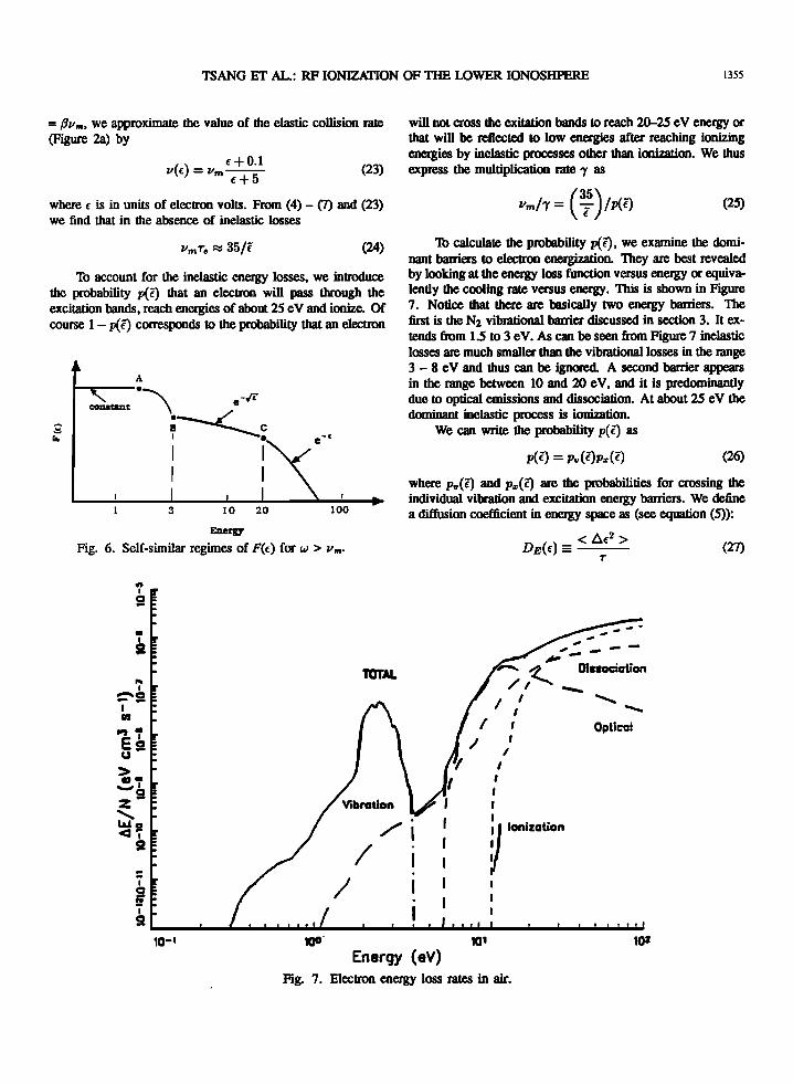
Th calculate the probability pel), we examine the domi­nant barriers to electron energization. They are best revealed by looking at the energy loss function versus energy or equiva­lendy the cooling rate versus energy. This is shown in Figure 7. Notice that there are basically two energy barriers. The first is the N2 vibrational barrier discussed in section 3. It ex­tends from 1.5 to 3 e V. As can be seen from Figure 7 inelastic losses are much smaller than the vibrational losses in the range 3 - 8 e V and thus can be ignored. A second barrier appears in the range between 10 and 20 eV, and it is predominandy due to optical emissions and dissociation. At about 25 eV the dominant inelastic process is ionization.

We can write the probability p( €) as

pC€) = p.,(€)p.,(€) (26)

where p.,(€) and p.,(l) are the probabilities for crossing the individual vibration and excitation energy barriers. We define a diffusion coefficient in energy space as (see equation (5»:

DE (f) == < flf2 > (27) T

" -----;-" DIssociation

/, ......... I ' I

I , , Optical

10'

I I , ,

I I

V ..... ·· ... • I

101

Energy (eV) Fig. 7. Electron energy loss rates in air.

1356 TSANG ET AL.: RF IONIZATION OF THE LOWER IONOSHPERE

The coefficient DE(f) is related to D(f) given by (2) by

DE(f) = fD(f,w,l) (28)

with the arguments w, l suppressed in DE(f). In the narrow energy rante of the vibrational resonance, DE(f) can be con­sidered as independent of energy and equal to DE(f = fV).

The energy diffusion time through the vibrational barrier of width 6.~, is

6.2

TD = DE(v) (29)

Therefore, if T~ = .1. is the time scale for vibrational exci-v. tation, the probability p~(l) that an electron will cross it will be given by

p~(l) ~ ezp [_ (T~~ ) 1/2] (30)

which using (28) and (29) becomes

p~(l) = ezp [-G V~:;:~~l) 1/2] (31)

Since v~ ~ 1/2 V(f~), f~ = 2.6 eV, and 6.~ ~ 1 eV, we find that

(32)

Perfonning a similar analysis for the excitation-dissociation barrier, with fIll ~ 14eV, 6.", ~ 6eV, and v.,/v(14eV) ~ 2 we find

(-) ( . ff.fill p., f = ezp -V ~ ) (33)

From (32) and (33) the total probability to cross the barrier will be

pel) = P~(l)P.,(l) = ezp ( _J2;V) (34)

Finally, from (25) and (34) we find

-y/vm = 3 x 1O-2ezp ( _J2 ;v) (35)

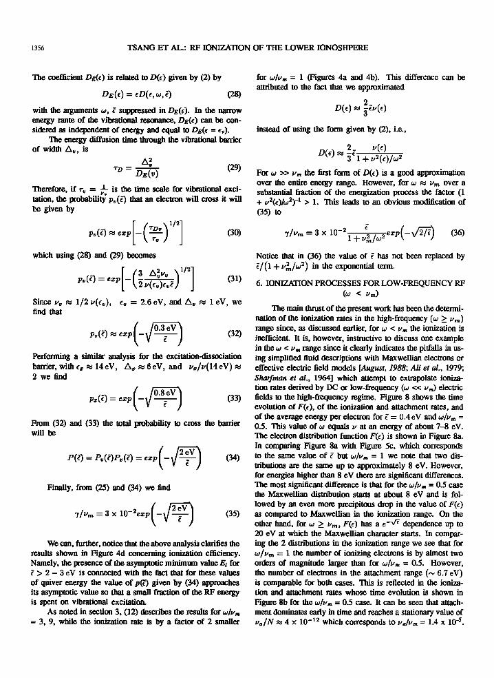
We can, further, notice that the above analysis clarifies the results shown in Figure 4d concerning ionization efficiency. Namely, the presence of the asymptotic minimum value E; for l > 2 - 3 e V is connected with the fact that for these values of quiver energy the value of p(l) given by (34) approaches its asymptotic value so that a small fraction of the RF energy is spent on vibrational excitation.

As noted in section 3, (12) describes the results for w/v", = 3, 9, while the ionization rate is by a factor of 2 smaller

for w/v'" = 1 (Figures 4a and 4b). This difference can be attributed to the fact that we approximated

D(f) ~ ~lV(f)

instead of using the form given by (2), i.e.,

D() 2_ V(f)

f ~ -f -:--:---:;;7'-;:-;--;; 3 1 + V2(f)/W2

For w » v'" the first form of D(l) is a good approximation over the entire energy range. However, for w ~ Vm over a substantial fraction of the energization process the factor (1 + v2(f)/w2>-1 > 1. This leads to an obvious modification of (35) to

(36)

Notice that in (36) the value of l has not been replaced by l/(1 + v;'.Iw2) in the exponential term.

6. IONIZATION PROCESSES FOR LOW-FREQUENCY RF (w < vm )

The main thrust of the present work has been the determi­nation of the ionization rates in the high-frequency (w ;:: v m )

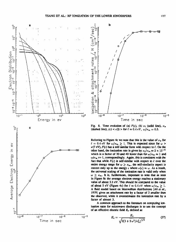
range since, as discussed earlier, for w < v'" the ionization is inefficient It is, however, instructive to discuss one example in the w < v 1ft range since it clearly indicates the pitfallS in us­ing simplified fluid descriptions with Maxwellian electrons or effective electric field models [August. 1988; Ali et al., 1979; Sharj'mIJn et al., 1964] which attempt to extrapolate ioniza­tion rates derived by DC or low-frequency (w « v".) electric fields to the high-frequency regime. Figure 8 shows the time evolution of F(l), of the ionization and attachment rates, and of the average energy per electron for l = 0.4 eV and w/vm = 0.5. This value of w equals v at an energy of about 7--8 eV. The electron distribution function F(f) is shown in Figure 8a. In comparing Figure Sa with Figure 5c, which corresponds to the same value of l but w/v", = 1 we note that two dis­tributions are the same up to approximately 8 eV. However, for energies higher than 8 eV there are significant differences. The most significant difference is that for the w/v", = 0.5 case the Maxwellian distribution starts at about 8 eV and is fol­lowed by an even more precipitous drop in the value of F(f) as compared to Maxwellian in the ionization range. On the other hand, for w ;:: Vm , F(l) has a e-,ff dependence up to 20 eV at which the Maxwellian character starts. In compar­ing the 2 distributions in the ionization range we see that for w / Vm = 1 the number of ionizing electrons is by almost two orders of magnitude larger than for w/v", = 0.5. However, the number of electrons in the attachment range ( ...... 6.7 eV) is comparable for both cases. This is reflected in the ioniza­tion and attachment rates whose time evolution is shown in Figure 8b for the w/v", = 0.5 case. It can be seen that attach­ment dominates early in time and reaches a stationary value of VaiN ~ 4 X 10-12 whiCh corresponds to va/v", = 1.4 x 10-5•

N o

o

o o

......, UJN .- 1 00

C 0", '-I """'0 U~ (])

Wv 1 o

If")

1 o

<0 1 o

> (])

C

>-0"> I... (]) C

W

o

Co 0 0 I...~ ...... U (])

W

(])

0"> o I... (])

> «

1 o

a

c

TSANG ET AL.: RF IONIZATION OF THE LOWER IONOSHPERE 1357

100 101

Energy In ev

10-7 10-6

Time In sec

.. , , .,

z

------~ 1 UJO (])~

-+-'

o I...

v ......,-C~ (])~

E .£:

I

I

I

b

/

I

I I

Fig. 8. Time evolution of (a) F(f.), (b) Vi (solid line), v" (dashed line), (c) < f.(t) > for l = 0.4 eV. w/vm = 0.5.

Referring to Figure 4c we note that this is the value of v" for l = 0.4 eV for w/vm ~ 1. This is expected since for W > v(7 eV), F(f.) has a self-similar form with respect to l. On the other hand, the ionization rate is given by v;/vm ~ 2 X 10-5

which is a factor of 20 and 40 lower than for w/vm ~ 1 and w/v .. » I, correspondingly. Again, this is consistent with the fact that while F(f.) is self-similar with respect to lover the entire energy range for W ~ V m • the self-similarity aspect is correct only up to the energy f. where Vet) ~ w. As a result, the universal scaling of the ionization rate is valid only when W ~ V m . It is, furthermore, important to note that as seen in Figure 8c the average electron energy reaches a stationary value of about 3.2 eV. This should be compared to the value of about 5 eV (Figure 4c) for l ~ 0.4 eV when w/vm ~ 1. A fluid model based on Maxwellian disbibutions [Ali el al., 1979] gives an attachment rate by a factor of 2 smaller than the observed, while it overestimates the ionization rate by a factor of almost 3.

A common approach to the literature on computing ion­ization rates for microwave discharges is to use the concept of an effective electric field E. defined as

E _ Eo

• - J2(1 + 2 W2/V"!,.) 1/2

(37)

1358 TSANG ET AL.: RF IONIZATION OF THE LOWER IONOSHPERE

The ionization mle IIJP or equivalently IIJN or IIJII., is then taken as a function of E.IP or equivalently E.III.,. This approach then uses ionization data derived from C elecbic field breakdown experiments to delennine the ionization rates for the equivalent C case using (34). This is equivalent to assuming that the electron distribution function F(f) is a self­similar function of E.III., over the aI1achment, ionization, and main inelastic loss (i.e., vibrational) range. H we define the parameter g as

(3S)

we find that

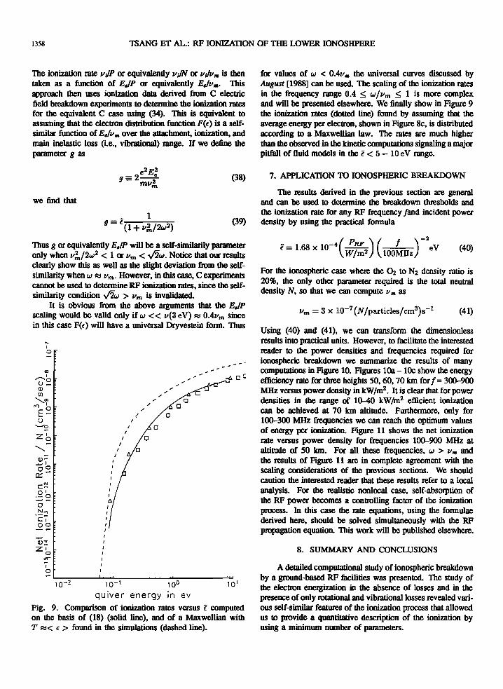
for values of w < 0.411., the universal curves discussed by August [1988] can be used. The scaling of the ionization rates in the frequency range 004 ~ W/llm ~ 1 is more complex and will be presented elsewhere. We finally show in Figure 9 the ionization rates (dotted line) found by assuming that the avemge energy per electron, shown in Figure Sc, is disbibuted according to a Maxwellian law. The mles are much higher than the observed in the kinetic computations signaling a major pitfall of fluid models in the f < 5 - 10 e V range.

7. APPLICATION TO IONOSPHERIC BREAKDOWN

The results derived in the previous section are general and can be used to determine the breakdown thresholds and the ionization rate for any RF frequency land incident power _ 1

9 = f (1 + 1I?n/2w2) (39) density by using the practical fonnula

Thus g or equivalently E.IP will be a self-similarily parameter only when 1I;'/2w2 < 1 or 11m < -/2w. Notice that OlD' results clearly show this as well as the slight deviation from the self­similarity when W ::::::I 11m. However, in this case, C experiments cannot be used to determine RF ionization rates, since the self­similarity condition -/2w > 11m is invalidaled.

It is obvious from the above arguments that the E.IP scaling would be valid only if w < < 11(3 eV) ::::::I Oo4llm since in this case F(f) will have a universal Dryveslein form. Thus

"" , o

., , '-""'0 u~ v (/)

.......... '" ,.,.,' E~ u

'-"'0

20 ~

..........

v-~,

o~ 0::

c::~ 0' .-0 ~~

a N., .--c::, ..2~ -v:: 2' 0 .....

'j' 0

10-2

I

I, "

,­,-

t 0

o

--'

10-1 100 10'

qUiver energy in ev Fig. 9. Comparison of ionization rates versus f computed on the basis of (IS) (solid line), and of a Maxwellian with T ::::::1< f > found in the simulations (dasbed line).

f= 1.68 x 10-4(:;:2) (100~IIZ) -2eV (40)

For the ionospheric case where the <h to N2 density ratio is 20%, the only other parameter required is the total neulrai density N, so that we can compute II", as

11m = 3 X 10-7 (N/particles/cm3)s-1 (41)

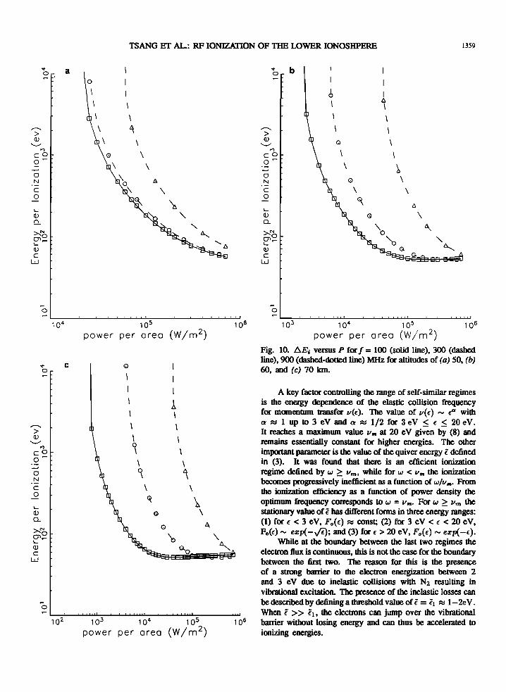
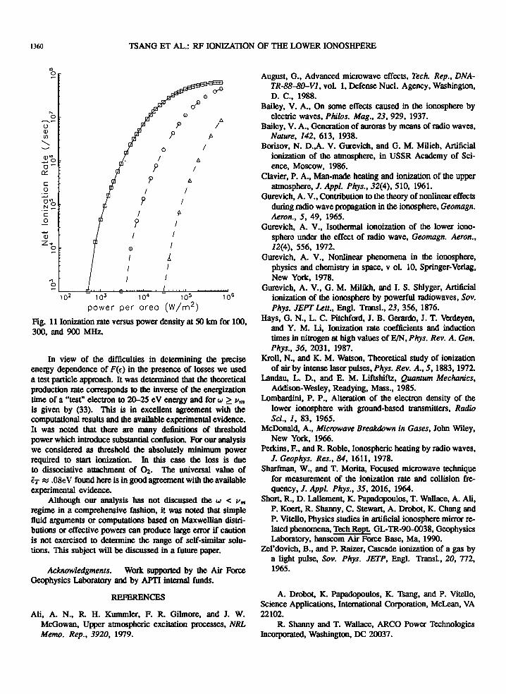
Using (40) and (41), we can transform the dimensionless results into practical units. However, 10 facilitate the interested reader to the power densities and frequencies required for ionospheric breakdown we summarize the results of many computations in Figure 10. Figures lOa - lOe show the energy efficiency rate for three heights 50, 60, 70 Ian for 1= 300-900 MHz versus power density in kW/m2. It is clear that for power densities in the range of 10-40 kW/m2 efficient ionization can be achieved at 70 Ian altitude. Furthermore, only for 100-300 MHz frequencies we can reach the optimum values of energy per ionization. Figure 11 shows the net ionization rate versus power density for frequencies 100-900 MHz at altitude of 50 km. For all these frequencies, w > II", and the results of Figure 11 are in complete agreement with the scaling considerations of the previous sections. We should caution the interested reader that these results refer to a local analysis. For the realistic nonlocal case, self-absorption of the RF power becomes a controlling factor of the ionization process. In this case the mle equations, using the formulae derived here, should be solved simultaneously with the RF propagation equation. This work will be published elsewhere.

8. SUMMARY AND CONCLUSIONS

A detailed computational study of ionospheric breakdown by a ground-based RF facilities was presented. The study of the electron energizalion in the absence of losses and in the presence of only rotational and vibrational losses revealed vari­ous self-similar features of the ionization process that allowed us to provide a quantitative description of the ionization by using a minimum number of parameters.

.... a 0 ~

------> Q)

'---'

'" CO o~

0 N

c 0

I.... Q)

0..

>-.'" O'~ '-Q)

c w

o

.... c o

.......... > Q)

'---'

'" CO o~

o N

C o "-Q) Q.

o

TSANG ET AL.: RF IONIZATION OF THE LOWER IONOSHPERE 1359

t I

\

\

\, L\ , \0 \

\ \

l!.

\

~ "-

" A.....

105

power per area (W/m2)

(j)

\

I

! \ \

\ \ \ ~

\ \

~ ~ , , ~ 'l!.

Q \

o

103 104 105

power per area (W / m 2)

.... b 0 ~

<1> I I:> \

\

------ \ > Q)

Q \ '---'

'" CO \ o~ ,

~ 0 , N 0 c \ \ 0

'-\ /!; I.... Q) Q \ 0...

l\ >-.'" CJ'I~ "-I.... 6...., Q)

c ~ /!;

w

o

106 103 104 105 106

power per area (W/m2)

Fig. 10. t:::..E; versus P for f = 100 (solid line), 300 (dashed line), 900 (dashed-dotted line) MHz for altitudes of (a) 50, (b) 60, and (c) 70 kIn.

A lcey factor controlling the range of self-similar regimes is the energy dependence of the elastic collision frequency for momentum transfer V(f). TIle value of V(f) "" fa with cr ~ 1 up to 3 eV and cr ~ 1/2 for 3 eV ~ f ~ 20 eV. It reaches a maximum value v'" at 20 eV given by (8) and remains essentially constant for higher energies. The other important parameter is the value of the quiver energy f defined in (3). It was found that there is an efficient ionization regime defined by w ~ V m • while for w < v'" the ionization becomes progressively inefficient as a function of wlv",. From the ionization efficiency as a function of power density the optimum frequency corresponds to w = V",. For w ~ Vm the stationary value of f has different forms in three energy ranges: (1) for f < 3 eV, Fo(f) ~ const; (2) for 3 eV < f < 20 eV, Fo(f) ..... ezp(-v'f); and (3) for f > 20 eV, Fo(f) "" ezp( -f).

While at the boundary between the last two regimes the electron Bux is continuous, this is not the case for the boundary between the first two. TIle reason for this is the presence of a strong barrier to the electron energization between 2 and 3 eV due to inelastic collisions with N2 resulting in vibrational excitation. The presence of the inelastic losses can be described by defining a threshold value off = fl ~ 1-2eV. When f » flo the electrons can jump over the vibrational barrier without losing energy and can thus be accelerated to ionizing energies.

1360 TSANG ET AL.: RF IONIZATION OF THE LOWER IONOSHPERE

u (]) en

., °

" °

"-.

(])'" ...... 0 O~

n:: c 0

...... 0'" NO

C 0

..., (])

z. °

'" ° ~ 102 - 103

power

0-0 0

~ I<)

? [;.

/ ? p.

0 /

/ 8

? / p I;

/

'f / y,.

? / I

0 I

I ~ I

I

104 105

per area (W/m2)

Fig. 11 Ionization rate versus power density at 50 km for 100, 300, and 900 MHz.

In view of the difficulties in detennining the precise energy dependence of F(e) in the presence of losses we used a test particle approach. It was detennined that the theoretical production rate corresponds to the inverse of the energization time of a "test" electron to 20-25 eV energy and for w ~ 11m

is given by (33). This is in excellent agreement with the computational results and the available experimental evidence. It was noted that there are many definitions of threshold power which introduce substantial confusion. For our analysis we considered as threshold the absolutely minimum power required to start ionization. In this case the loss is due to dissociative attachment of~. The universal value of fT ~ .08e V found here is in good agreement with the available experimental evidence.

Although our analysis has not discussed the w < II",

regime in a comprehensive fashion, it was noted Ihat simple fluid arguments or computations based on Maxwellian distri­butions or effective powers can produce large error if caution is not exercised to detennine the range of self-similar solu­tions. This subject will be discussed in a future paper.

Acknowledgments. Work supported by the Air Force Geophysics Laboratory and by APT! intemal funds.

REFERENCES

Ali, A. N., R. H. Kummler, F. R. Gilmore, and J. W. McGowan, Upper atmospheric excitation processes, NRL Memo. Rep., 3920, 1979.

August, G., Advanced microwave effects, Tech. Rep., DNA­TR-88--8O-Vl, voL I, Defense Nucl. Agency, Washington, D. C., 1988.

Bailey, V. A., On some effects caused in the ionosphere by electric waves, Philos. Mag., 23, 929, 1937.

Bailey, V. A., Generation of auroras by means of radio waves, Nature, 142, 613, 1938.

Borisov, N. D.,A. V. Gurevich, and G. M. Milieh, Artificial ionization of the atmosphere, in USSR Academy of Sci­ence, Moscow, 1986.

Clavier, P. A., Man-made heating and ionization of the upper atmosphere, J. Appl. Phys., 32(4), 510, 1961.

Gurevich, A. V., Contribution to the theory of nonlinear effects during radio wave propagation in the ionosphere, Geomagn. Aeron., 5, 49, 1965.

Gurevich, A. V., Isothermal ionoization of the lower iono­sphere under the effect of radio wave, Geomagn. Aeron., 12(4), 556, 1972.

Gurevich, A. V., Nonlinear phenomena in the ionosphere, physics and chemistry in space, v 01. 10, Springer-Verlag, New York, 1978.

Gurevich, A. V., G. M. Milikh, and I. S. Shlyger, Artificial ionization of the ionosphere by powerful radiowaves, Sov. Phys. JEPT Lett., Engl. Transl., 23, 356, 1876.

Hays, G. N., L. C. Pitchford, J. B. Gerardo, J. T. Verdeyen, and Y. M. Li, Ionization rate coefficients and induction times in nitrogen at high values ofEIN, Phys. Rev. A. Gen. Phys., 36, 2031, 1987.

Kroll, N., and K. M. Watson, Theoretical study of ionization of air by intense laser pulses, Phys. Rev. A., 5, 1883, 1972.

Landau, L. D., and E. M. Liftshiftz, Quantum Mechanics, Addison-Wesley, Readying, Mass., 1985.

Lombardini, P. P., Alteration of the electron density of the lower ionosphere with ground-based transmitters, Radio Sci., I, 83, 1965.

McDonald, A., Microwave Breakdown in Gases, John Wiley, New York, 1966.

Perkins, F., and R. Roble, Ionospheric heating by radio waves, J. Geophys. Res., 84, 1611, 1978.

Sharfman, W., and T. Morita, Focused microwave technique for measurement of the ionization rate and collision fre­quency, J. Appl. Phys., 35, 2016, 1964.

Short, R., D. Lallement, K. Papadopoulos, T. Wallace, A. Ali, P. Koert, R. Shanny, C. Stewart, A. Drobot, K. Chang and P. Vitello, Physics studies in artificial ionosphere mirror re­lated phenomena, Tech RepL GL-TR-90--0038, Geophysics Laboratory, hanscom Air Force Base, Ma, 1990.

Zel'dovich, B., and P. Raizer, Cascade ionization of a gas by a light pulse, Sov. Phys. JETP, Engl. Transl., 20, 772, 1965.

A. Drobot, K. Papadopoulos, K. Tsang, and P. Vitello, Science Applications, International Corporation, McLean, VA 22102.

R. Shanny and T. Wallace, ARCO Power Technologies Incorporated, Washington, DC 20037.