RF-Based Relative Localization for Robot Swarmsnkamra/pdf/locrobot.pdf · RF-Based Relative Localization for Robot Swarms Wolfgang Honig¨ 1, Nitin Kamra Abstract—We evaluate the

RF-Based Relative Localization for Robot Swarms

Wolfgang Honig1, Nitin Kamra1

Abstract— We evaluate the radio signal strength indicator(RSSI) of an nRF5188 based robot swarm for relative localiza-tion. We discuss an efficient way of high-speed data collectionwith up to 40,000 RSSI samples per second. Semi-automatic ra-dio parameter selection as well as robot-assisted data collectionmethods are presented. Furthermore, we show our collecteddata including the variance for selected outdoor experiments.The resulting data is used to fit a novel sigmoid based powervs. log-distance model, which in turn is the foundation of acentralized anchor-free localization algorithm. We present asimple gradient descent based localization approach which iscomputationally simple, easily extensible to distributed swarms,and scales efficiently to large number of robots in a swarm.

I. INTRODUCTIONLocalization remains a hard problem in robotics. Using

multiple robots which are able to localize each other can helpfor formation control and improve the global localizationof the group (for example, if one of the robots has accessto GPS-based localization). The signal strength of radiocommunication correlates with the distance between thesender and receiver. Assuming a 2D plane, the formation canbe reconstructed up to orientation and mirror uncertainties ifall robot-to-robot distances are known.

The scope of the project is to evaluate whether the RF-chip of the Crazyflie 2.0 quadrotor can be used as foundationfor the relative localization for a small swarm of robots ina simplified 2D-plane setting. We consider the case of staticnodes (Crazyflies) on the ground and attempt to do a relativelocalization for each Crazyflie using only RSSI data from itsneighbors.

II. RELATED WORKLocalization for swarms has mainly been discussed in

the Wireless Sensor Networks (WSNs) literature. Recentsurveys [1], [2] classify the research in this field either bymeasurement techniques (such as Time of Flight or signalstrength), or localization approach (self-localization or targetlocalization).

For our work, we will focus on related work which eitheruses the radio signal strength indicator (RSSI) or discussesself-localization algorithms. In general, the problem of lo-calization with RSSI data can be divided into two phases:

1) Retrieve distance information from RSSI data.2) Estimate positions from pairwise distance information

using some optimization algorithm.Retrieving distance information from RSSI readings has

been attempted in literature using both deterministic func-tions and stochastic methods. The most common approach

1Authors are with the Department of Computer Science, University ofSouthern California, USA {whoenig, nkamra}@usc.edu

to model the RSSI vs. distance function is by using a Log-distance path loss model [3]. It assumes that measured RSSIdecreases linearly with log10 d and models uncertainty in thisprocess by imposing a zero-mean gaussian noise on top ofthe straight line. Furthermore the model has been extendedwith a dynamic variance (LNSM-DV) [4].

After retrieving the function (or probability distribution)relating RSSI and distance, the next step involves solvingfor exact 2-D or 3-D coordinates using pairwise distancedata which can be done by formulating the problem asan optimization problem. A large portion of the wirelesslocalization literature revolves around ways to solve theresulting optimization problem.

Moore et al. use fairly accurate (5 cm) sonar-based dis-tance sensors to achieve relative localization between movingrobots using a distributed algorithm [5]. They employ asimple computational approach to find quadrilaterals in alocal neighborhood which are robust to noise and thencompute relative transformations between local clusters, allof which can be done in O(n3) time using efficient datastructures. While the algorithm shows good theoretical andpractical results, it is questionable if it will work for the kindof data we obtain using RSSI, which suffers from fading andinterference effects and as such has a lot of noise.

RSSI-based approaches often use so-called beacons oranchor nodes, which are nodes deployed at a fixed and knownposition. Zanca et al. compare different RSSI-based methodswith varying number of anchor nodes in an indoor setting [6].The results suggest an expected accuracy of about 2m with 5anchor nodes using a Maximum Likelihood approximation.On the contrary, we want to analyze the possibility ofusing RSSI measurements without anchor nodes for relativelocalization.

Another set of approaches to localization derive their in-spiration from biological swarms. Kulkarni et al. [7] presenta comparison of the two most popular bio-inspired opti-mization algorithms: Particle Swarm Optimization (PSO) andBacterial Foraging Algorithm (BFA) in terms of the numberof nodes localized, localization accuracy and computationtime.

In this work we propose a smooth sigmoid function tomodel the variation of RSSI vs. distance and then present asimple gradient descent based optimization approach whichis computationally simple, easily extensible to distributedswarms and scales efficiently to large number of robots in aswarm.

III. TARGET PLATFORM

The Bitcraze Crazyflie 2.0 Nano Quadcopter [8] is a flyingdevelopment kit that targets researchers and hobbyists. Itweighs about 27 g, is about 92mm motor to motor, and fitsin the palm of a human hand. The software and hardwarespecifications are freely available online, which makes theplatform great for research.

The Crazyflie has a dual-MCU architecture using annRF5188 (Cortex-M0, 32MHz, 16 kB SRAM, 128 kBflash) for power management and communication and anSTM32F405 (Cortex-M4, 168MHz, 192 kB SRAM, 1MBflash) for the control algorithm. Both MCUs are connectedusing UART. Sensors include the MPU9250 (gyroscope,accelerometer, magnetometer) and a LPS25H (pressure). Thesetpoint (yaw, pitch, roll, thrust) can be sent from a PC usinga special USB dongle, or using BlueTooth LE.

The radio chip nRF51822 is a SoC which is able touse BlueTooth Smart and custom 2.4GHz wireless radiocommunication. It is possible to communicate over 127different channels in the 2.4GHz band and it supportsRSSI (Received Signal Strength Indicator) with an accuracyof ±6 dB (resolution of 1 dB [9, Table 42]). Additionally,the power amplifier for the RF communication is softwarecontrolled.

IV. APPROACH TO DATA COLLECTION

In the following we will describe the various steps whichwere taken in order to collect RSSI data between differentCrazyflies.

A. Implementing PTX mode and RSSI measurements

With the default firmware every Crazyflie acts as primaryreceiver (PRX), while the PC-side (using the USB-DongleCrazyradio) operates as primary transmitter (PTX). Theprimary transmitter can send a data packet, which will bereceived by the receiver and acknowledged using up to32Bytes in the acknowledgment packet. For communicatingwithin the swarm, it is required that each Crazyflie canoperate in PTX mode as well. This mode is not implementedin the default firmware. Therefore, we used a library by thechip vendor [10] initially, however it turned out to be not agood fit for two reasons:

1) The queues for sending and receiving are completelyindependent, i.e. it is impossible to send the correctacknowledgment packet immediately as a response.This asynchronous protocol behavior made higher-level communication primitives much more compli-cated and error-prone.

2) While low-frequency RSSI sampling was supported,adding a special high-frequency sample mode was toocomplicated due to the complexity of the library code.

Nevertheless, working code based on this library can befound in one of our branches1.

1https://github.com/whoenig/Crazyflie2-nrf-firmware/tree/cs599_ptx

To overcome the above discussed limitations, we imple-mented our own radio driver2. A callback mechanism allowsto acknowledge packets immediately, as long as the requiredcomputation is very small (the callback has to be calledduring an interrupt handler). Furthermore, we implementedhigh frequency RSSI sampling with up to 60,000 samples persecond. This data is filtered to only take those data pointsinto account where the radio is in receive mode, the Crazyfliedevice address matches the packet header, and a correctCRC was sent. In practice, this reduces the sampling toabout 40,000 samples per second if the transmitting Crazyflietransmits as fast as possible.

We use a hybrid approach to stream the data out. First, thedata is averaged on chip, by computing the count and sumduring every RSSI interrupt. Both count and sum are sentvia SEGGERs Real Time Terminal [11] using a SEGGERJ-Link EDU every 10ms. This requires the Crazyflie DebugAdapter Kit which contains a small PCB to be soldered onthe Crazyflie to obtain an SWD debug adapter port. On thePC side small python scripts are used to receive, plot, andstore the data.

B. Parameter selection: Power, Datarate, Channel

The radio allows to select eight different trans-mit power levels (4 dBm, 0 dBm, −4 dBm, −8 dBm,−12 dBm, −16 dBm, −20 dBm, −30 dBm), three datarates(250Kbit/s, 1Mbit/s, 2Mbit/s), and 127 channels whichcorrespond to a carrier frequency. It is expected that allthose parameters do not alter the obtained RSSI significantly,and hence it should be possible to select a fixed set ofparameters. We did three different experiments to validatethis assumption.

First, we implemented a special powerscan mode in thefirmware, which automatically switches between all availabletransmit power levels and collects the RSSI values. Thesevalues were recorded at different distances indoors. TheCrazyflies were placed manually in a room equipped witha motion capture system at different distances and valueswere recorded once the data stabilized. The results arevisible in Fig. 1(a) and show that there is just a fixed offsetbetween the power levels as expected. However, there is alsoa saturation visible for very short distances. Therefore, weselected −8 dBm as power level for future experiments.

Second, we implemented a similar mode for the differentdata rates. There was no visible change in the RSSI valuesand we choose the slowest possible mode. This maximizesthe number of RSSI samples we get during communication,because the samples are taken at a fixed frequency indepen-dent of the data rate.

Third, we implemented a special channelscan mode whichcollects the RSSI values for all available channels whilekeeping the distance constant. Due to multi-path interferenceand other signals on the 2.4GHz band (such as WiFi), a highvalue does not necessary mean a strong signal. Therefore we

2https://github.com/whoenig/Crazyflie2-nrf-firmware/tree/cs599_datacollection

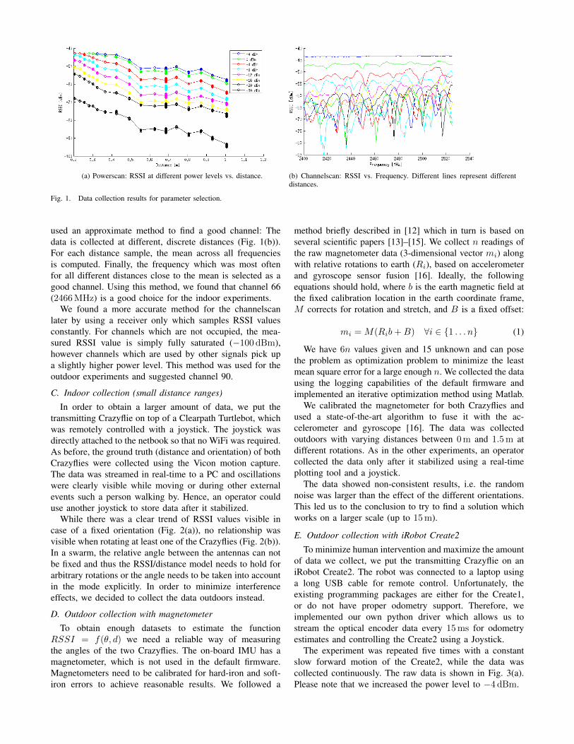
(a) Powerscan: RSSI at different power levels vs. distance. (b) Channelscan: RSSI vs. Frequency. Different lines represent differentdistances.

Fig. 1. Data collection results for parameter selection.

used an approximate method to find a good channel: Thedata is collected at different, discrete distances (Fig. 1(b)).For each distance sample, the mean across all frequenciesis computed. Finally, the frequency which was most oftenfor all different distances close to the mean is selected as agood channel. Using this method, we found that channel 66(2466MHz) is a good choice for the indoor experiments.

We found a more accurate method for the channelscanlater by using a receiver only which samples RSSI valuesconstantly. For channels which are not occupied, the mea-sured RSSI value is simply fully saturated (−100 dBm),however channels which are used by other signals pick upa slightly higher power level. This method was used for theoutdoor experiments and suggested channel 90.

C. Indoor collection (small distance ranges)

In order to obtain a larger amount of data, we put thetransmitting Crazyflie on top of a Clearpath Turtlebot, whichwas remotely controlled with a joystick. The joystick wasdirectly attached to the netbook so that no WiFi was required.As before, the ground truth (distance and orientation) of bothCrazyflies were collected using the Vicon motion capture.The data was streamed in real-time to a PC and oscillationswere clearly visible while moving or during other externalevents such a person walking by. Hence, an operator coulduse another joystick to store data after it stabilized.

While there was a clear trend of RSSI values visible incase of a fixed orientation (Fig. 2(a)), no relationship wasvisible when rotating at least one of the Crazyflies (Fig. 2(b)).In a swarm, the relative angle between the antennas can notbe fixed and thus the RSSI/distance model needs to hold forarbitrary rotations or the angle needs to be taken into accountin the mode explicitly. In order to minimize interferenceeffects, we decided to collect the data outdoors instead.

D. Outdoor collection with magnetometer

To obtain enough datasets to estimate the functionRSSI = f(θ, d) we need a reliable way of measuringthe angles of the two Crazyflies. The on-board IMU has amagnetometer, which is not used in the default firmware.Magnetometers need to be calibrated for hard-iron and soft-iron errors to achieve reasonable results. We followed a

method briefly described in [12] which in turn is based onseveral scientific papers [13]–[15]. We collect n readings ofthe raw magnetometer data (3-dimensional vector mi) alongwith relative rotations to earth (Ri), based on accelerometerand gyroscope sensor fusion [16]. Ideally, the followingequations should hold, where b is the earth magnetic field atthe fixed calibration location in the earth coordinate frame,M corrects for rotation and stretch, and B is a fixed offset:

mi =M(Rib+B) ∀i ∈ {1 . . . n} (1)

We have 6n values given and 15 unknown and can posethe problem as optimization problem to minimize the leastmean square error for a large enough n. We collected the datausing the logging capabilities of the default firmware andimplemented an iterative optimization method using Matlab.

We calibrated the magnetometer for both Crazyflies andused a state-of-the-art algorithm to fuse it with the ac-celerometer and gyroscope [16]. The data was collectedoutdoors with varying distances between 0m and 1.5m atdifferent rotations. As in the other experiments, an operatorcollected the data only after it stabilized using a real-timeplotting tool and a joystick.

The data showed non-consistent results, i.e. the randomnoise was larger than the effect of the different orientations.This led us to the conclusion to try to find a solution whichworks on a larger scale (up to 15m).

E. Outdoor collection with iRobot Create2

To minimize human intervention and maximize the amountof data we collect, we put the transmitting Crazyflie on aniRobot Create2. The robot was connected to a laptop usinga long USB cable for remote control. Unfortunately, theexisting programming packages are either for the Create1,or do not have proper odometry support. Therefore, weimplemented our own python driver which allows us tostream the optical encoder data every 15ms for odometryestimates and controlling the Create2 using a Joystick.

The experiment was repeated five times with a constantslow forward motion of the Create2, while the data wascollected continuously. The raw data is shown in Fig. 3(a).Please note that we increased the power level to −4 dBm.

(a) RSSI vs. distance using fixed orientations of the Crazyflies. (b) RSSI vs. distance using varying orientations of the Crazyflies.

Fig. 2. Indoor data collection within small distances, using channel 66, −8dBm, and 250Kbit/s.

V. MODEL FITTING

The most common model used to fit RSSI data is theLog-distance path loss model [3]. It models the receivedRSSI reading (P ) as a straight line function of log10(d) withsuperimposed gaussian noise. The gaussian noise parameterscan be assumed constants or varying with distance. Themodel is given by:

P = P0 − γ log10 d+Xg (2)

In general, this model works well within a range ofdistance d1 ≤ d ≤ d2, but the RSSI readings get saturatedoutside this distance range. So we use a piecewise linear(PWL) model which follows the Log-distance path lossmodel between the cutoffs d1 and d2, but imposes a saturatedreading outside the range i.e.

P =

P0 − γ log10 d1 +Xg, d ≤ d1P0 − γ log10 d+Xg, d1 ≥ d ≥ d2P0 − γ log10 d2 +Xg, d2 ≤ d

(3)

For parameter estimation, we choose the values d1, d2, P0

and γ which maximize the log-likelihood of occurrence ofour data set. We iteratively search for the cutoffs d1 and d2,while computing P0 and γ every time using gradient descentfor each pair (d1, d2) and finally retain the best choices.Figure 3(a) shows our dataset and the fitted piecewise linearmodel.

Though the piecewise linear model is a good fit formaking predictions, it is not a good model to use in anyoptimization since it is not smooth. We aim to develop adecentralized localization algorithm later on, and most robotsare not sophisticated enough to run complicated non-linearoptimization techniques. Hence it is important to have asmooth, continuous and differentiable model for RSSI vs.log10 d fit, so that even robots with low computation power

can use the localization algorithm while employing a simplegradient descent for optimization.

For this reason, we came up with another model todescribe the RSSI vs. log10 d data. We model our data witha sigmoid curve which takes the following form:

P = PL +PH − PL

1 + e−s(log10 d−µ)+Xg (4)

The sigmoid function is a continuous and differentiablefunction and hence has nice properties with respect to differ-entiation. To the authors’ knowledge, this model has not beenused in the localization literature up till now. The sigmoidfit to our dataset has been shown in Fig. 3(b). It is clear thatnot only does the model fit better to the data now, but alsopermits the use of local gradient-based optimization methodsfor localization later on. Since Xg is distributed normally, weneed its mean and standard deviation as functions of distance,but for most practical purposes the mean can be set to 0, andthe standard deviation can be assumed constant. It can beobserved from Fig. 3(c) that the best-fit straight line has anaverage standard deviation of about 4 dBm, which we willuse as a measure of standard deviation for our model.

VI. CENTRALIZED LOCALIZATION

We used our model to conduct experiments for relativelocalization with a swarm of six Crazyflies. Though we laterintend to have a full decentralized localization algorithm,we currently solved the localization problem in a centralizedway.

The swarm of Crazyflies was kept in a static configurationindoors and we allotted each of them a unique ID. The ideawas to let them exchange RSSI data amongst themselves,which would then be streamed out to a PC and a localizationalgorithm run on it.

−0.8 −0.6 −0.4 −0.2 0 0.2 0.4 0.6 0.8 1 1.2−120

−110

−100

−90

−80

−70

−60

−50

−40

−30

distance [log(m)]

rssi

[dB

m]

(a) Fitting a piecewise linear model to RSSI dataset.

−0.8 −0.6 −0.4 −0.2 0 0.2 0.4 0.6 0.8 1 1.2−120

−110

−100

−90

−80

−70

−60

−50

−40

−30

distance [log(m)]

rssi

[dB

m]

(b) Fitting a sigmoid model to RSSI dataset.

−0.8 −0.6 −0.4 −0.2 0 0.2 0.4 0.6 0.8 1 1.20

2

4

6

8

10

12

14

distance [log(m)]

stdd

ev [d

Bm

]

(c) Std. deviation as a function of distance about the fitted sigmoid.

Fig. 3. Model fitting to RSSI dataset.

A. ApproachEach Crazyflie was pre-programmed to transmit at

−4 dBm, 250KBit/s and 2490MHz, and ran a state ma-chine which initialized all of them in a wait to synchronizemode. On receiving the synchronize signal from a PC, allof them would start their clocks together and go into asignaling mode. In this mode, the Crazyflies took turnstransmitting messages (containing their ID) one-by-one inthe order of their unique IDs while all other Crazyflies wouldlisten and measure RSSI signal strength. This way eachCrazyflie would end up having signal strength data fromeach of their neighbors. This stage was followed by a datasharing stage, where each Crazyflie would transmit all itssignal strength data to a PC, where it would be fed to alocalization algorithm.

B. Problem FormulationUsing our sigmoid model for RSSI data, we now formu-

late the problem of localization as a maximum likelihoodproblem. Table I shows the notation used in this paper.

Given a set of readings for n Crazyflies in the format:[TxID,RxID,Pij], the problem of relative localization is

n Number of CrazyfliesTxID Transmitter Crazyflie IDRxID Receiver Crazyflie IDPij RV representing RSSI value with TxID = i and RxID = jpij RSSI value with TxID = i and RxID = jXi RV representing x-coordinate of ith Crazyfliexi x-coordinate of ith CrazyflieYi RV representing y-coordinate of ith Crazyflieyi y-coordinate of ith CrazyflieDij RV representing distance between ith and jth Crazyfliesdij Distance between ith and jth CrazyfliesAij 1 if pij value is available, 0 otherwiseN (i) Set of neighbors of Crazyflie with ID = i

TABLE I. Notation used in this paper (RV = Random Variable).

of determining the euclidean coordinates (xi, yi) of eachCrazyflie from the above data. We formulate this problemas a maximum likelihood problem as follows:

maxx,yP(P = p|X = x and Y = y) (5)

Since all readings are independent, the above can be writtenas a product of probabilities of occurring of individual

readings.

maxx,y

∏i,j

j∈N (i)

P(Pij = pij |Xi = xi, Yi = yi, Xj = xj , Yj = yj)

(6)Using our sigmoid model with gaussian noise, this can bewritten as:

maxx,y

∏i,j

j∈N (i)

1√2πσ

e− 1

2σ2

(pij−PL−

PH−PL1+e

−s(log10 dij−µ)

)2

(7)

where

dij =√(xi − xj)2 + (yi − yj)2 (8)

Since σ has been assumed independent of distance (andhence of x and y), we can ignore it and further transform theproblem to a minimization problem by taking negative-logof the objective function.

minx,y

1

2

∑i

∑j∈N (i)

(pij − PL −

PH − PL1 + e−s(log10 dij−µ)

)2

(9)

Now considering the sigmoid function as:

g(z) = PL +PH − PL

1 + e−s(z−µ)(10)

and letting Aij denote the availability of the value pij , wecan write the above minimization problem as follows:

minx,y

F (x, y)

where

F (x, y) =1

2

∑i

∑j

Aij (pij − g(log10 dij))2

(11)

C. Optimizing with Gradient Descent

To optimize our objective function (11), we use a simplegradient descent algorithm. But to compute the gradient ofF (x, y), we first need the following derivatives:

∂dij∂xi

= −∂dij∂xj

=xi − xjdij

(12)

∂dij∂yi

= −∂dij∂yj

=yi − yjdij

(13)

We have the derivative of sigmoid function as:

d(g(z))

dz=s(PH − PL)e−s(z−µ)

(1 + e−s(z−µ))2(14)

which can be re-written as follows:

d(g(z))

dz=s(g(z)− PL)(PH − g(z))

PH − PL(15)

With the above derivatives in place, we can now calculatethe gradient of F (x, y) as follows:

∂F (x, y)

∂xk= −∑j

{Akj (pkj − g(log10 dkj))

s(g(log10 dkj)− PL)(PH − g(log10 dkj))PH − PL

(xk − xj)d2kj log 10

}−∑i

{Aik (pik − g(log10 dik))

s(g(log10 dik)− PL)(PH − g(log10 dik))PH − PL

(xk − xi)d2ik log 10

}(16)

∂F (x, y)

∂yk= −∑j

{Akj (pkj − g(log10 dkj))

s(g(log10 dkj)− PL)(PH − g(log10 dkj))PH − PL

(yk − yj)d2kj log 10

}−∑i

{Aik (pik − g(log10 dik))

s(g(log10 dik)− PL)(PH − g(log10 dik))PH − PL

(yk − yi)d2ik log 10

}(17)

The above gradient equations are correct assuming thatAkk = 0 ∀k.

Finally we can implement the gradient descent in aniterative loop as shown in algorithm 1. α is the step-sizefactor and can be fine-tuned to speed up or slow down theconvergence of the algorithm.

1: Initialize x, y randomly2: repeat3: xk := xk − α∂F (x,y)

∂xk∀k

4: yk := yk − α∂F (x,y)∂yk

∀k5: until convergence

Algorithm 1. Gradient Descent Algorithm

VII. RESULTS AND DISCUSSION

Preliminary tests with randomly generated RSSI values(including noise) showed that our centralized localizationalgorithm can find the correct solution. One of the nodes wasalways held fixed at the origin to avoid convergence issuesdue to absence of a global reference frame. This avoideda global translation ambiguity in the solution, however thesolution does suffer from global reflection and rotationambiguities. Seeding the initial values with a noisy guessof the actual solution often derived a very close match if thestandard deviation of the super-imposed noise was not verylarge.

Results for a run of the centralized localization algorithmcan be seen in Fig. 4. The data for this experiment wascreated by placing six nodes randomly and generating their

−3.5 −3 −2.5 −2 −1.5 −1 −0.5 0 0.5 1−3

−2

−1

0

1

2

3

4

X [m]

Y [m

]

Actual locationsPredicted locations

Fig. 4. Results of Centralized localization with 6 nodes and randomlyallotted locations. The data was created by adding zero-mean gaussian noisewith 4dBm std. deviation to the RSSI readings generated by the sigmoidmodel. A noisy estimate of the actual locations was provided to seed theoptimization algorithm. The algorithm does not give a very accurate estimatefinally because of the added noise in the RSSI readings.

pairwise RSSI readings according to our sigmoid model. Azero-mean gaussian noise of std. deviation 4 dBm was addedto the RSSI readings before giving them to the optimizationalgorithm. The algorithm was seeded with a close (butrandom) initial estimate of the nodes’ locations. As canbe observed from the figure, the algorithm does produceestimates close to the actual positions. It could not convergeto the actual positions because of the noise in RSSI readings.

Further tests with actual data did not work out that welland the algorithm did not find a close match. There are manypossible causes for this behavior:• The algorithm should behave better with a large number

of nodes but we were limited by the number of availablerobots to six nodes.

• The Crazyflies have slightly different RSSI vs. distancecurves based on their actual antenna placement, chipvariations etc. Nevertheless, the model had been createdusing a specific single pair of Crazyflies and not for allof them. So it would be useful to create a model whichtakes the individual transmission and reception poweroffsets of each Crazyflie into account, by accepting themas input parameters.

• Finally, our approach assumes a constant variance,while Fig. 3(c) suggests that the variance is actuallyincreasing with distance and the variation of RSSI withdistance should be included in the model as well.

VIII. FUTURE WORKFuture work on this project would proceed along the lines

of obtaining better models and filtering the acquired data.More specifically we wish to do a histogram-based data

collection [17] which rejects the lower and upper 25% RSSIsamples at each distance before computing an average. Thisleads to better noise rejection for the collected samples.

Another way to improve the model-fitting could be to dooutlier rejection on the dataset first. It is clear from figures3(a) and 3(b) that there are many outliers at every distanceand rejecting them would give us a better model representingthe data.

Moreover we currently include only those readings in ouroptimization objective where pij is available. But if pij isnot available, it signifies that Crazyflies i and j are probablyfar apart and this information can also be considered inthe optimization objective to make the localization moreaccurate.

Lastly, since each Crazyflie is slightly different, we wouldlike to model the individual transmission and receptionoffsets of the wireless nodes (Crazyflies) as pointed out insection VII.

REFERENCES

[1] G. Mao, B. Fidan, and B. D. Anderson, “Wireless sensornetwork localization techniques,” Computer Networks, vol. 51,no. 10, pp. 2529 – 2553, 2007. [Online]. Available: http://www.sciencedirect.com/science/article/pii/S1389128606003227

[2] G. Han, H. Xu, T. Duong, J. Jiang, and T. Hara, “Localizationalgorithms of wireless sensor networks: a survey,” TelecommunicationSystems, vol. 52, no. 4, pp. 2419–2436, 2013. [Online]. Available:http://dx.doi.org/10.1007/s11235-011-9564-7

[3] T. S. Rappaport, Wireless Communications: Principles and Practice,2nd ed. Prentice Hall, 2002.

[4] J. Xu, W. Liu, F. Lang, Y. Zhang, and C. Wang, “Distance measure-ment model based on rssi in wsn,” Wireless Sensor Network, vol. 2,no. 08, p. 606, 2010.

[5] D. Moore, J. Leonard, D. Rus, and S. Teller, “Robust distributednetwork localization with noisy range measurements,” in Proceedingsof the 2Nd International Conference on Embedded Networked SensorSystems, ser. SenSys ’04. New York, NY, USA: ACM, 2004, pp. 50–61. [Online]. Available: http://doi.acm.org/10.1145/1031495.1031502

[6] G. Zanca, F. Zorzi, A. Zanella, and M. Zorzi, “Experimentalcomparison of rssi-based localization algorithms for indoor wirelesssensor networks,” in Proceedings of the Workshop on Real-world Wireless Sensor Networks, ser. REALWSN ’08. NewYork, NY, USA: ACM, 2008, pp. 1–5. [Online]. Available:http://doi.acm.org/10.1145/1435473.1435475

[7] R. Kulkarni, G. Venayagamoorthy, and M. Cheng, “Bio-inspirednode localization in wireless sensor networks,” in Systems, Man andCybernetics, 2009. SMC 2009. IEEE International Conference on, Oct2009, pp. 205–210.

[8] Crazyflie nano quadcopter. [Online]. Available: http://www.bitcraze.se[9] “nRF51822 product specification v3.1,” Nordic Semiconductor, Oslo,

Norway.[10] Stripped down enhanced shockburst library for the nrf51

series. [Online]. Available: https://github.com/NordicSemiconductor/nrf51-micro-esb

[11] Real time terminal. [Online]. Available: https://www.segger.com/jlink-real-time-terminal.html

[12] Calibration part 5: Magnetometers (continued). [Online]. Available:https://myahrs.wordpress.com/2012/04/19/calibration-part-5/

[13] M. Kok, J. Hol, T. Schon, F. Gustafsson, and H. Luinge, “Calibrationof a magnetometer in combination with inertial sensors,” in Informa-tion Fusion (FUSION), 2012 15th International Conference on, July2012, pp. 787–793.

[14] V. Renaudin, M. H. Afzal, and G. Lachapelle, “Complete TriaxisMagnetometer Calibration in the Magnetic Domain,” Journalof Sensors, vol. 2010, pp. 1–10, 2010. [Online]. Available:http://dx.doi.org/10.1155/2010/967245

[15] J. Vasconcelos, G. Elkaim, C. Silvestre, P. Oliveira, and B. Cardeira,“Geometric approach to strapdown magnetometer calibration in sensorframe,” Aerospace and Electronic Systems, IEEE Transactions on,vol. 47, no. 2, pp. 1293–1306, April 2011.

[16] S. Madgwick, A. Harrison, and R. Vaidyanathan, “Estimation of imuand marg orientation using a gradient descent algorithm,” in Reha-bilitation Robotics (ICORR), 2011 IEEE International Conference on,June 2011, pp. 1–7.

[17] A. Awad, T. Frunzke, and F. Dressler, “Adaptive distance estimationand localization in wsn using rssi measures,” in Digital System DesignArchitectures, Methods and Tools, 2007. DSD 2007. 10th EuromicroConference on, Aug 2007, pp. 471–478.

APPENDIX A: SOURCE CODE

Crazyflie firmware changes

The code can be found online (including compilation andusage instructions):

NRF51 Firmware: PTX Mode based on Micro-ESB: Thisfirmware uses [10] to implement both PTX and PRX mode.https://github.com/whoenig/

Crazyflie2-nrf-firmware/tree/cs599_ptx

NRF51 Firmware: Datacollection: This firmware usesa custom driver for the radio. It supports power, datarate,and channel scanning as well as a streaming mode forcontinuous data collection for fixed power level, datarate,and channel. In combination with the STM32 compassfirmware, it is possible to collect the orientation based onthe magnetometer as well.https://github.com/whoenig/

Crazyflie2-nrf-firmware/tree/cs599_datacollection

NRF51 Firmware: Centralized Localization: Thisfirmware listens to a signal from the PC in order tosynchronize clocks, collect pairwise RSSI signal strengthin the whole swarm, and sends the results back to the PCfor centralized localization. Hence, it can be used for puredata collection as well without the need of a special debugadapter.https://github.com/whoenig/

Crazyflie2-nrf-firmware/tree/cs599_master

NRF51 Firmware: (Improved) Channelscan: Thisfirmware contains an improved channelscan which doesnot require a special transmitter. Instead, it continuouslymeasures signal strength (without filtering) for differentchannels and sends the data to the PC using SEGGERs RealTime Terminal.https://github.com/whoenig/

Crazyflie2-nrf-firmware/tree/channelscan

STM32 Firmware: Compass Support: This firmware (forthe STM32) allows to read the raw magnetometer data,uses a given calibration model to correct the values, andsends them to the NRF51 using UART for data collectionpurposes.https://github.com/whoenig/Crazyflie-firmware/tree/

cs599_master

Scripts

The following scripts are part of a private github reposi-tory.• iRobot Create2:

https://github.com/whoenig/cs599project/blob/

master/scripts/Create2.py

• Model Fitting:https://github.com/whoenig/cs599project/tree/

master/scripts/Model%20learning

• Centralized Localization:https://github.com/whoenig/cs599project/tree/

master/scripts/Centralized%20Optimization

• Magnetometer Calibration:https://github.com/whoenig/cs599project/tree/

master/scripts/magnetometer