Revisiting the Southern Pine Growth Decline

Revisiting the Southern Pine Growth Decline: Where Are We

10 Years Later?

Gary L. Gadbury Michael S. WilliamsHans T. Schreuder

United StatesDepartmentof Agriculture

Forest Service

Rocky MountainResearch Station

General TechnicalReport RMRS-GTR-124

February 2004

USDA Forest Service RMRS-GTR-124. 2004 1

Gadbury, Gary L.; Williams, Michael S.; Schreuder, Hans T. 2004. Revisiting the southern pine growth de-cline: Where are we 10 years later? Gen. Tech. Rep. RMRS-GTR-124. Fort Collins, CO: U.S. Department of Agriculture, Forest Service, Rocky Mountain Research Station. 10 p.

Abstract

This paper evaluates changes in growth of pine stands in the state of Georgia, U.S.A., using USDA Forest Service Forest Inventory and Analysis (FIA) data. In particular, data representing an additional 10-year growth cy-cle has been added to previously published results from two earlier growth cycles. A robust regression procedure is combined with a bootstrap technique to produce estimates of mean growth with confidence intervals for the fourth, fifth, and sixth inventories of natural pine stands sampled between 1961 and 1990. Results suggest that sixth cycle growth rates of pine stands in Georgia remain fairly constant with rates observed in the fifth growth cy-cle, though they are not up to the level of growth observed in the fourth cycle. Overall, we conclude that growth in the stands screened for this analysis declined between the fourth and fifth cycles but stabilized in the sixth cycle. Inferences cannot be extended to the entire state of Georgia but only to the unknown population represented by the screened dataset of undisturbed natural pine stands. We highlight some specifics on what can and cannot be inferred from FIA data and recommend future actions to increase the chance of detecting changes and revealing factors that might be associated with the changes. The recent switch in FIA to annualized inventories will make it more likely that changes such as these will be easier to detect and interpret in the future.

Key words: bootstrap, cause-effect, forest inventory and analysis, robust regression

The Authors

Gary L. Gadbury is an associate professor of statistics at the University of Missouri at Rolla, Missouri. Michael S. Williams and Hans T. Schreuder are mathematical statisticians for the USDA Forest Service Rocky Mountain Research Station at Fort Collins, Colorado.

You may order additional copies of this publication by sending your mailing information in label form through one of the following media. Please specify the publication title and series number.

Fort Collins Service Center

Telephone (970) 498-1392 FAX (970) 498-1396 E-mail [email protected] Web site http://www.fs.fed.us/rm Mailing address Publications Distribution

Rocky Mountain Research Station 240 West Prospect Road Fort Collins, CO 80526

Rocky Mountain Research StationNatural Resources Research Center

2150 Centre Avenue, Building AFort Collins, CO 80526

Cover: Natural stand of 40-year-old loblolly pine by David J. Moorhead, The University of Georgia, www.forestryimages.org.

mailto:[email protected]

USDA Forest Service RMRS-GTR-124. 2004 1

Introduction

A controversial topic related to U.S. forest inventories was the southern pine growth decline issue in the 1980s. The U.S. Forest Service Forest Inventory and Analysis (FIA) program indicated that the growth of natural pines in Georgia and Alabama in the 1970s had decreased sig-nificantly from levels reported in the 1960s. In various newspapers articles, this was attributed to pollution.

FIA inventories were never designed to assess true cause and effect (Schreuder and Thomas 1991), just as the linkage between smoking and lung cancer could not be unequivocally confirmed from the numerous survey studies that suggested a connection between the two. Careful experimentation finally conclusively estab-lished such a link. Establishing cause-effect from obser-vational survey data is difficult (Gadbury and Schreuder 2003). Although cause and effect is beyond the scope of FIA, the FIA survey is suitable for assessing change in the forest resource over large areas. We document, as well as possible, what can be concluded from FIA data, a new procedure for analyzing FIA data, and a reanalysis that incorporates an additional growth cycle.

Literature Review

The FIA program, initiated in 1928, inventories the forest resources of the United States and regularly pro-duces population estimates such as the total area of for-est and timber volume as well as change over time. Until recently, FIA was a periodic inventory where states were visited one at a time every 7-22 years. A decline in growth of natural southern pine timber volume from the fourth cycle (1961-1971) to the fifth cycle (1972-1982) was observed primarily in Georgia and Alabama. Concerns arose regarding the use of FIA data to con-clude a growth decline. However, the findings were supported by several researchers (Sheffield and others 1985; Sheffield and Cost 1987). The decline in growth was reported to be as much as 17-23% for natural loblol-ly pine and 27% for natural shortleaf pine (Zahner and others 1989; Bechtold and others 1991).

Ruark and others (1991) used FIA data to compare the periodic annual increment in basal area of selected naturally regenerated pine stands throughout Alabama

and Georgia. Estimated growth rates between 1972 and 1982 (fifth cycle) were compared with estimated growth rates obtained during the previous 10-year survey cy-cle (fourth cycle). Separate analyses were conducted for loblolly, longleaf, shortleaf, and slash pine cover types. Comparisons of growth rates yielded reductions ranging from 3% to 31% in both states. All reductions were sta-tistically significant except for the 3% decline in natu-ral loblolly pine in Alabama. Bechtold and others (1991) performed a similar study that focused only on the state of Georgia. Both Bechtold and others (1991) and Ruark and others (1991) developed models that adjusted the observed growth rates for changes in stand structure. T-tests were used to evaluate the significance of mean adjusted growth rates obtained from analysis of covari-ance models. The conclusion from both papers was that the declines could not be attributed to changes involving the modeled stand structural parameters; however, the agent(s) causing the decline were not identified.

A number of other studies examined possible expla-nations of a decline in growth. Knight (1987) attributed the decline to four factors: declining area of timberland, inadequate regeneration after harvest on non-industrial private forest lands, increased tree mortality, and a re-duction in the rate of tree and stand growth. Zahner and others (1989), collecting tree-ring data on a 10% sub-sample of FIA field plots across the Piedmont region of Georgia, North Carolina, and South Carolina, developed tree-ring models to interpret the growth decline of lob-lolly pine. These authors attributed some of the decline to region-wide drought periods between 1950 and 1959 and again between 1980 and 1983. Another important factor identified was the increase in average basal area and number of stems per hectare. This study concluded that the annual growth rate of trees in the early 1980s was about two-thirds that of trees growing in similar conditions 35 years earlier. Moreover, it concluded that a significant portion of the decline could not be attribut-ed to either climatic or stand conditions but speculated that high levels of ozone in the region could have been a significant factor.

Czaplewski and others (1994) used the Georgia FIA data to look at spatial patterns to determine if atmospher-ic deposition from large metropolitan areas could be a factor in a growth decline. While there was a significant

Revisiting the Southern Pine Growth Decline: Where Are We 10 Years Later?

Gary L. Gadbury, Michael S. Williams, and Hans T. Schreuder

2 USDA Forest Service RMRS-GTR-124. 2004 USDA Forest Service RMRS-GTR-124. 2004 3

spatial pattern associated with the growth decline, this pattern could also be explained by an unusually slow-growing cluster of pine plots in the mountains approxi-mately 100 km north of Atlanta. However, after using a regression model to adjust for local stand conditions, no significant spatial autocorrelation existed.

A number of concerns were raised regarding these findings. Hyink (1991), in a response to Bechtold and others (1991), was concerned about the differences in the distributions of age and site classes in data screened from the two growth cycles. He also noted that there was a troubling number of plots with atypically high growth rates in the fourth cycle in Georgia and that there is a lack of knowledge regarding what constitutes a “nor-mal” growth rate for natural pine stands in the region.

Gertner (1991) commented on the analysis techniques used by Bechtold and others (1991) by noting that there are likely to be large amounts of error in some of the independent variables when a calibrated model is used to adjust mean logarithmic growth. He concludes that while there may have been a real reduction in growth rates, the possibility that the reduction may have result-ed from biases caused by sampling errors and data trans-formations could not be ruled out.

Some of these concerns were addressed in subse-quent studies. Ouyang and others (1991) used bootstrap and jackknife methods for inference since distribu-tions of residuals from fitted models were often “heavy tailed.” Ueng and others (1997) used a robust regres-sion technique to minimize the influence of outlying re-siduals from fitted models. Gadbury and others (1998, 2002) used classification and regression tree methods to account for possible complex nonlinear relationships among variables describing growth, mortality, and stand structure. The results of each of these studies agreed with the results of Bechtold and others (1991) and Ruark and others (1991). Thus, some of the earlier concerns over the methods of analyses did not invalidate the findings.

Zeide (1992) performed an extensive analysis of data from the third to sixth cycles and pointed out that the re-ported changes were puzzling in light of the fact that the decline occurred only for naturally regenerated pines, but was unobserved in pine plantations. He suggested that either there was a growth decline before 1961, or more likely that there was no evidence of a growth de-cline and that the data were deficient for several reasons: (1) a drastic change from the fixed area plot sampling to variable radius plot sampling, (2) the presence of numer-ous outliers, and (3) inconsistencies in relationships be-tween variables.

As noted in Schreuder and Thomas (1991) and af-firmed in comments to that article by Clutter and Hyink

(1991), screening of the data as done in both the Georgia and Georgia/Alabama studies make it difficult to assess the actual population for inference. So, was there a de-cline in growth in natural pine stands in the period from the 1960s to the 1970s? We believe there was for the screened data analyzed, but extension of these results to the entire population of natural pine stands in Georgia and Alabama is not warranted. What should be done to maximize the possibility of identifying and assessing meaningful hypotheses of change in the future and pos-sible causes for them? We address that in the section on recommendations at the end of the paper.

Where Are We Today?

Some things have changed. First and foremost is the addition of the sixth cycle to the FIA inventory. From these data, the growth rate between the fifth and sixth cy-cle can be estimated and compared to that of the fourth. There are also new analytical techniques. Recently FIA procedures have changed drastically by going from a cy-clical inventory to an annualized inventory where 20% of the plots will be measured in each state each year. FIA has also integrated with the Forest Health Monitoring (FHM) program and has dedicated a systematic sub-set of its plot network to investigating issues related to forest health (Stolte 2001). Ten years of research into cause-effect issues with FIA data has improved our understanding of the problem and going to an annual-ized inventory has provided us with improved ability to assess change. The goals of this study are to:

• Introduce robust methods for analyzing data from pe-riodic surveys.

• Compare the growth rates between the fourth, fifth, and sixth cycles of the inventory to see whether per-ceived declines continued into the sixth cycle.

• Recommend possible methods to analyze such data in the future.

• Identify issues that arise when attempting to use ob-servational data to attribute an observed change to po-tentially “causal” factors.

• Identify what can and cannot be accomplished with FIA-type observational data.

Data Description

Three types of naturally regenerating pine stands were studied and were designated by their domi-nant species: loblolly (Pinus taeda), shortleaf (Pinus echinata), and slash pine (Pinus elliottii). The data


represent growth rates and stand structure of forest plots in Georgia over three 10-year periods span-ning the years 1961-1990. The three periods are referred to as the fourth, fifth, and sixth growth cycles. The data for cycles prior to the fourth were not suitable for assessing changes in growth rates. Additional information about the data can be found in Bechtold and others (1991).

Each growth cycle uses an independent sam-ple of forest plots because the time lapse between samples and drastic changes in stand structure and disturbances made it unrealistic to follow the same plots over the three growth cycles. A total sample size of 692 loblolly plots was obtained, 235 from the fourth cycle, 104 from the fifth cycle, and 353 from the sixth, of which 11 were common to all three cycles. A total sample size of 258 shortleaf plots was obtained, 127 from the fourth cycle, 45 from the fifth, and 86 from the sixth, of which three were common to all three. Finally, a total sample size of 401 slash pine plots was obtained, 84 from the fourth cycle, 83 from the fifth, and 234 from the sixth, of which seven were common to all three. The plots common to all three growth cycles rep-resented a small fraction of the total sample, and so they too were treated as independent observations across the three cycles.

The variables of interest are: GG = gross annual basal area growth per acre (survivor growth + ingrowth); S = site index representing volume growth potential (S rep-resents a relation between age and height of dominant and co-dominant pines in each stand (base 50 years); A = stand age (midpoint of 10 year class); N = number of stems per acre; P = ratio of yellow pine basal area per acre to basal area of all species; M = annual basal area mortality per acre of trees alive at initial inventory that die from natural causes prior to terminal inventory; net growth denoted NG, equal to GG – M . GG, N, M, and NG are all based on trees 1.0 inches dbh and larger at the time of the initial inventory.

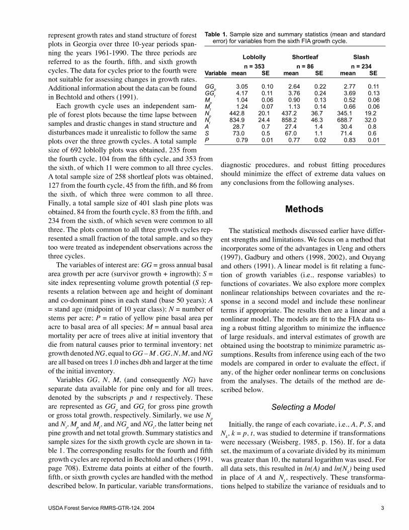
Variables GG, N, M, (and consequently NG) have separate data available for pine only and for all trees, denoted by the subscripts p and t respectively. These are represented as GGp and GGt for gross pine growth or gross total growth, respectively. Similarly, we use Np and Nt, Mp and Mt, and NGp and NGt, the latter being net pine growth and net total growth. Summary statistics and sample sizes for the sixth growth cycle are shown in ta-ble 1. The corresponding results for the fourth and fifth growth cycles are reported in Bechtold and others (1991, page 708). Extreme data points at either of the fourth, fifth, or sixth growth cycles are handled with the method described below. In particular, variable transformations,

diagnostic procedures, and robust fitting procedures should minimize the effect of extreme data values on any conclusions from the following analyses.

Methods

The statistical methods discussed earlier have differ-ent strengths and limitations. We focus on a method that incorporates some of the advantages in Ueng and others (1997), Gadbury and others (1998, 2002), and Ouyang and others (1991). A linear model is fit relating a func-tion of growth variables (i.e., response variables) to functions of covariates. We also explore more complex nonlinear relationships between covariates and the re-sponse in a second model and include these nonlinear terms if appropriate. The results then are a linear and a nonlinear model. The models are fit to the FIA data us-ing a robust fitting algorithm to minimize the influence of large residuals, and interval estimates of growth are obtained using the bootstrap to minimize parametric as-sumptions. Results from inference using each of the two models are compared in order to evaluate the effect, if any, of the higher order nonlinear terms on conclusions from the analyses. The details of the method are de-scribed below.

Selecting a Model

Initially, the range of each covariate, i.e., A, P, S, and Nk, k = p, t, was studied to determine if transformations were necessary (Weisberg, 1985, p. 156). If, for a data set, the maximum of a covariate divided by its minimum was greater than 10, the natural logarithm was used. For all data sets, this resulted in ln(A) and ln(Nk) being used in place of A and Nk, respectively. These transforma-tions helped to stabilize the variance of residuals and to

Table 1. Sample size and summary statistics (mean and standard error) for variables from the sixth FIA growth cycle.

Loblolly Shortleaf Slash

n = 353 n = 86 n = 234Variable mean SE mean SE mean SE

GGp 3.05 0.10 2.64 0.22 2.77 0.11

GGt 4.17 0.11 3.76 0.24 3.69 0.13

Mp 1.04 0.06 0.90 0.13 0.52 0.06

Mt 1.24 0.07 1.13 0.14 0.66 0.06

Np 442.8 20.1 437.2 36.7 345.1 19.2

Nt 834.9 24.4 858.2 46.3 688.7 32.0

A 28.7 0.7 27.4 1.4 30.4 0.8S 73.0 0.5 67.0 1.1 71.4 0.6P 0.79 0.01 0.77 0.02 0.83 0.01


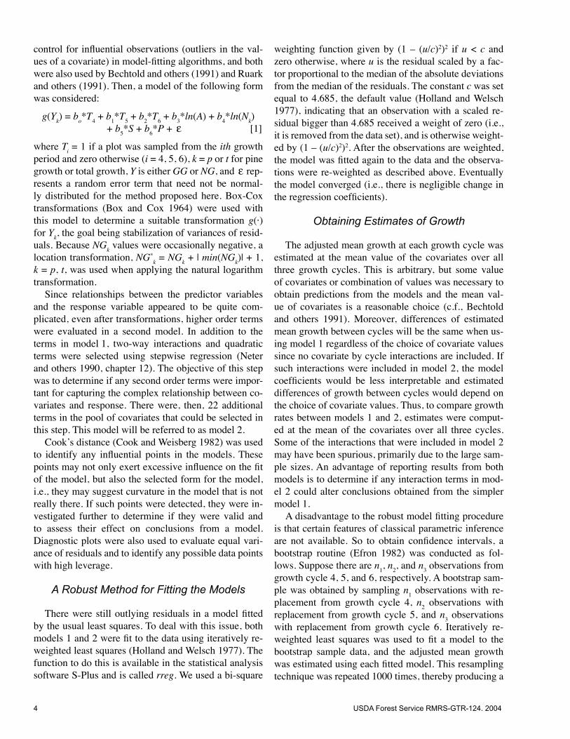
control for influential observations (outliers in the val-ues of a covariate) in model-fitting algorithms, and both were also used by Bechtold and others (1991) and Ruark and others (1991). Then, a model of the following form was considered:

g(Yk) = bo*T4 + b1*T5 + b2*T6 + b3*ln(A) + b4*ln(Nk) + b5*S + b6*P + ε [1]

where Ti = 1 if a plot was sampled from the ith growth period and zero otherwise (i = 4, 5, 6), k = p or t for pine growth or total growth, Y is either GG or NG, and ε rep-resents a random error term that need not be normal-ly distributed for the method proposed here. Box-Cox transformations (Box and Cox 1964) were used with this model to determine a suitable transformation g(·) for Yk, the goal being stabilization of variances of resid-uals. Because NGk values were occasionally negative, a location transformation, NG*

k = NGk + | min(NGk)| + 1, k = p, t, was used when applying the natural logarithm transformation.

Since relationships between the predictor variables and the response variable appeared to be quite com-plicated, even after transformations, higher order terms were evaluated in a second model. In addition to the terms in model 1, two-way interactions and quadratic terms were selected using stepwise regression (Neter and others 1990, chapter 12). The objective of this step was to determine if any second order terms were impor-tant for capturing the complex relationship between co-variates and response. There were, then, 22 additional terms in the pool of covariates that could be selected in this step. This model will be referred to as model 2.

Cook’s distance (Cook and Weisberg 1982) was used to identify any influential points in the models. These points may not only exert excessive influence on the fit of the model, but also the selected form for the model, i.e., they may suggest curvature in the model that is not really there. If such points were detected, they were in-vestigated further to determine if they were valid and to assess their effect on conclusions from a model. Diagnostic plots were also used to evaluate equal vari-ance of residuals and to identify any possible data points with high leverage.

A Robust Method for Fitting the Models

There were still outlying residuals in a model fitted by the usual least squares. To deal with this issue, both models 1 and 2 were fit to the data using iteratively re-weighted least squares (Holland and Welsch 1977). The function to do this is available in the statistical analysis software S-Plus and is called rreg. We used a bi-square

weighting function given by (1 – (u/c)2)2 if u < c and zero otherwise, where u is the residual scaled by a fac-tor proportional to the median of the absolute deviations from the median of the residuals. The constant c was set equal to 4.685, the default value (Holland and Welsch 1977), indicating that an observation with a scaled re-sidual bigger than 4.685 received a weight of zero (i.e., it is removed from the data set), and is otherwise weight-ed by (1 – (u/c)2)2. After the observations are weighted, the model was fitted again to the data and the observa-tions were re-weighted as described above. Eventually the model converged (i.e., there is negligible change in the regression coefficients).

Obtaining Estimates of Growth

The adjusted mean growth at each growth cycle was estimated at the mean value of the covariates over all three growth cycles. This is arbitrary, but some value of covariates or combination of values was necessary to obtain predictions from the models and the mean val-ue of covariates is a reasonable choice (c.f., Bechtold and others 1991). Moreover, differences of estimated mean growth between cycles will be the same when us-ing model 1 regardless of the choice of covariate values since no covariate by cycle interactions are included. If such interactions were included in model 2, the model coefficients would be less interpretable and estimated differences of growth between cycles would depend on the choice of covariate values. Thus, to compare growth rates between models 1 and 2, estimates were comput-ed at the mean of the covariates over all three cycles. Some of the interactions that were included in model 2 may have been spurious, primarily due to the large sam-ple sizes. An advantage of reporting results from both models is to determine if any interaction terms in mod-el 2 could alter conclusions obtained from the simpler model 1.

A disadvantage to the robust model fitting procedure is that certain features of classical parametric inference are not available. So to obtain confidence intervals, a bootstrap routine (Efron 1982) was conducted as fol-lows. Suppose there are n1, n2, and n3 observations from growth cycle 4, 5, and 6, respectively. A bootstrap sam-ple was obtained by sampling n1 observations with re-placement from growth cycle 4, n2 observations with replacement from growth cycle 5, and n3 observations with replacement from growth cycle 6. Iteratively re-weighted least squares was used to fit a model to the bootstrap sample data, and the adjusted mean growth was estimated using each fitted model. This resampling technique was repeated 1000 times, thereby producing a


sampling distribution of adjusted mean growth estimates for each growth cycle and for each model. A family of three 95% confidence intervals was constructed for the mean growth at each growth cycle using a Bonferroni correction so that each individual interval had a 98.3% confidence level, i.e., since we are simultaneously es-timating mean growth at three growth cycles, an indi-vidual confidence interval will have a confidence level of 100(1 – 0.05/3) = 98.3% (c.f., Christensen 1996, sec-tion 6.2). Using the bootstrapped sampling distribution, the eighth and 992nd sorted values represent the boot-strapped lower and upper confidence limits. See Efron and Tibshirani (1993, chapter 13) for more details on percentile bootstrap confidence intervals. Growth esti-mates from both models were transformed back to the original arithmetic units.

Results

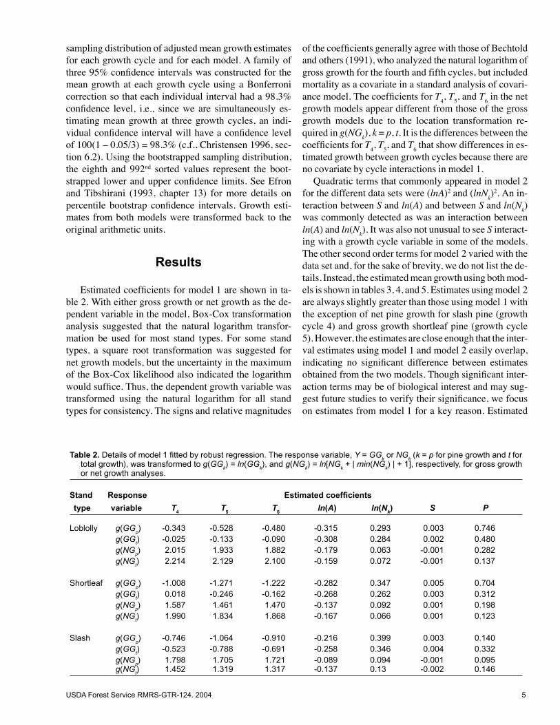
Estimated coefficients for model 1 are shown in ta-ble 2. With either gross growth or net growth as the de-pendent variable in the model, Box-Cox transformation analysis suggested that the natural logarithm transfor-mation be used for most stand types. For some stand types, a square root transformation was suggested for net growth models, but the uncertainty in the maximum of the Box-Cox likelihood also indicated the logarithm would suffice. Thus, the dependent growth variable was transformed using the natural logarithm for all stand types for consistency. The signs and relative magnitudes

of the coefficients generally agree with those of Bechtold and others (1991), who analyzed the natural logarithm of gross growth for the fourth and fifth cycles, but included mortality as a covariate in a standard analysis of covari-ance model. The coefficients for T4, T5, and T6 in the net growth models appear different from those of the gross growth models due to the location transformation re-quired in g(NGk), k = p, t. It is the differences between the coefficients for T4, T5, and T6 that show differences in es-timated growth between growth cycles because there are no covariate by cycle interactions in model 1.

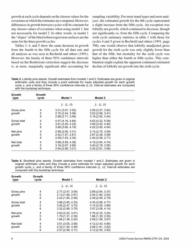
Quadratic terms that commonly appeared in model 2 for the different data sets were (lnA)2 and (lnNk)

2. An in-teraction between S and ln(A) and between S and ln(Nk) was commonly detected as was an interaction between ln(A) and ln(Nk). It was also not unusual to see S interact-ing with a growth cycle variable in some of the models. The other second order terms for model 2 varied with the data set and, for the sake of brevity, we do not list the de-tails. Instead, the estimated mean growth using both mod-els is shown in tables 3, 4, and 5. Estimates using model 2 are always slightly greater than those using model 1 with the exception of net pine growth for slash pine (growth cycle 4) and gross growth shortleaf pine (growth cycle 5). However, the estimates are close enough that the inter-val estimates using model 1 and model 2 easily overlap, indicating no significant difference between estimates obtained from the two models. Though significant inter-action terms may be of biological interest and may sug-gest future studies to verify their significance, we focus on estimates from model 1 for a key reason. Estimated

Table 2. Details of model 1 fitted by robust regression. The response variable, Y = GGk or NG

k (k = p for pine growth and t for

total growth), was transformed to g(GGk) = ln(GG

k), and g(NG

k) = ln[NG

k + | min(NG

k) | + 1], respectively, for gross growth

or net growth analyses.

Stand Response Estimated coefficients

type variable T4 T

5 T

6 ln(A) ln(N

k) S P

Loblolly g(GGp) -0.343 -0.528 -0.480 -0.315 0.293 0.003 0.746

g(GGt) -0.025 -0.133 -0.090 -0.308 0.284 0.002 0.480

g(NGp) 2.015 1.933 1.882 -0.179 0.063 -0.001 0.282

g(NGt) 2.214 2.129 2.100 -0.159 0.072 -0.001 0.137

Shortleaf g(GGp) -1.008 -1.271 -1.222 -0.282 0.347 0.005 0.704

g(GGt) 0.018 -0.246 -0.162 -0.268 0.262 0.003 0.312

g(NGp) 1.587 1.461 1.470 -0.137 0.092 0.001 0.198

g(NGt) 1.990 1.834 1.868 -0.167 0.066 0.001 0.123

Slash g(GGp) -0.746 -1.064 -0.910 -0.216 0.399 0.003 0.140

g(GGt) -0.523 -0.788 -0.691 -0.258 0.346 0.004 0.332

g(NGp) 1.798 1.705 1.721 -0.089 0.094 -0.001 0.095

g(NGt) 1.452 1.319 1.317 -0.137 0.13 -0.002 0.146


growth at each cycle depends on the chosen values for the covariates at which the estimates are computed. However, differences in growth between cycles will be constant for any chosen values of covariates when using model 1, but not necessarily for model 2. In other words, in model 1 the “slopes” of the fitted robust regression surfaces are the same for the three growth cycles.

Tables 3, 4, and 5 show the same decrease in growth from the fourth to the fifth cycle for all data sets and all analyses as was seen in Bechtold and others (1991). However, the family of three 95% confidence intervals based on the Bonferroni correction suggest the decrease is, at most, marginally significant after accounting for

sampling variability. For most stand types and most anal-yses, the estimated growth for the 6th cycle represented a slight increase from the fifth cycle. An exception was loblolly net growth, which continued to decrease, though not significantly so, from the fifth cycle. Comparing the sixth cycle summary statistics in table 1 with those for cycles 4 and 5 given in Bechtold and others (1991, page 708), one would observe that loblolly unadjusted gross growth for the sixth cycle was only slightly lower than that of the fifth, but mortality for the sixth cycle was higher than either the fourth or fifth cycles. This com-bination might explain the apparent continued estimated decline of loblolly net growth into the sixth cycle.

Table 3. Loblolly pine stands. Growth estimates from models 1 and 2. Estimates are given in original arithmetic units and they include a point estimate for mean adjusted growth for each growth cycle, $µ, and a family of three 95% confidence intervals (L,U). Interval estimates are computed with the bootstrap technique.

Growth Growth type cycle Model 1 Model 2

$µ , (L, U) $µ, (L, U)

Gross pine 4 3.31,(3.07, 3.55) 3.59,(3.27, 3.92) growth 5 2.75,(2.44, 3.08) 3.03,(2.68, 3.41) 6 2.89,(2.71, 3.06) 3.19,(2.92, 3.44)

Gross total 4 4.47,(4.16, 4.84) 4.63,(4.22, 5.09)growth 5 3.81,(3.45, 4.22) 3.95,(3.52, 4.40) 6 3.98,(3.80, 4.19) 4.22,(3.92, 4.54)

Net pine 4 2.99,(2.65, 3.31) 3.15,(2.75, 3.59)growth 5 2.42,(1.97, 2.81) 2.67,(2.28, 3.09) 6 2.09,(1.83, 2.34) 2.40,(2.06, 2.71)

Net total 4 3.98,(3.58, 4.38) 4.18,(3.64, 4.74)growth 5 3.19,(2.67, 3.69) 3.40,(2.78, 3.95) 6 2.94,(2.68, 3.21) 3.24,(2.81, 3.66)

Table 4. Shortleaf pine stands. Growth estimates from models 1 and 2. Estimates are given in original arithmetic units and they include a point estimate for mean adjusted growth for each growth cycle, $µ, and a family of three 95% confidence intervals (L, U). Interval estimates are computed with the bootstrap technique.


$µ, (L, U) $µ, (L, U)

Gross pine 4 2.77,(2.47, 3.05) 2.99,(2.64, 3.37)growth 5 2.13,(1.69, 2.61) 2.04,(1.60, 2.63) 6 2.23,(1.95, 2.56) 2.39,(2.06, 2.79)


Net pine 4 2.63,(2.22, 3.01) 2.76,(2.33, 3.24)growth 5 1.79,(1.31, 2.39) 1.86,(1.29, 2.55) 6 1.84,(1.38, 2.24) 2.09,(1.56, 2.67)

Net total 4 3.51,(3.05, 3.95) 4.12,(3.43, 4.85)growth 5 2.33,(1.54, 3.26) 2.68,(1.61, 3.82) 6 2.57,(2.08, 3.11) 3.12,(2.50, 3.83)


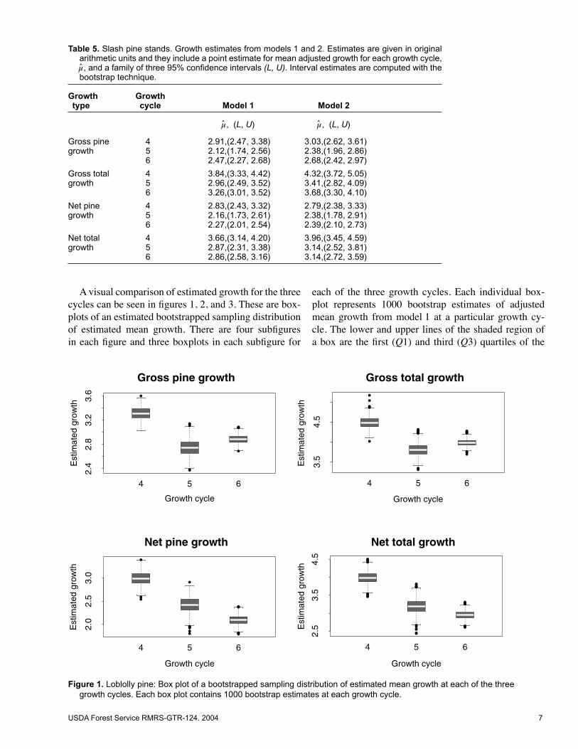
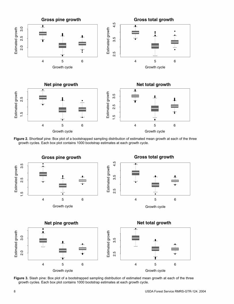
A visual comparison of estimated growth for the three cycles can be seen in figures 1, 2, and 3. These are box-plots of an estimated bootstrapped sampling distribution of estimated mean growth. There are four subfigures in each figure and three boxplots in each subfigure for

each of the three growth cycles. Each individual box-plot represents 1000 bootstrap estimates of adjusted mean growth from model 1 at a particular growth cy-cle. The lower and upper lines of the shaded region of a box are the first (Q1) and third (Q3) quartiles of the

Table 5. Slash pine stands. Growth estimates from models 1 and 2. Estimates are given in original arithmetic units and they include a point estimate for mean adjusted growth for each growth cycle, $µ, and a family of three 95% confidence intervals (L, U). Interval estimates are computed with the bootstrap technique.


$µ, (L, U) $µ, (L, U)

Gross pine 4 2.91,(2.47, 3.38) 3.03,(2.62, 3.61)growth 5 2.12,(1.74, 2.56) 2.38,(1.96, 2.86) 6 2.47,(2.27, 2.68) 2.68,(2.42, 2.97)


Net pine 4 2.83,(2.43, 3.32) 2.79,(2.38, 3.33)growth 5 2.16,(1.73, 2.61) 2.38,(1.78, 2.91) 6 2.27,(2.01, 2.54) 2.39,(2.10, 2.73)

Net total 4 3.66,(3.14, 4.20) 3.96,(3.45, 4.59)growth 5 2.87,(2.31, 3.38) 3.14,(2.52, 3.81) 6 2.86,(2.58, 3.16) 3.14,(2.72, 3.59)

2.4

2.8

3.2

3.6 •

••

•••

•

••••

4 5 6

Growth cycle

Est

imat

ed g

row

th

Gross pine growth

3.5

4.5

•

•••••

••

•••••••••

••••

•••••

4 5 6

Growth cycle

Est

imat

ed g

row

th

Gross total growth

2.0

2.5

3.0

••

•

••••••

•

••••

•••

4 5 6

Growth cycle

Est

imat

ed g

row

th

Net pine growth

2.5

3.5

4.5

••••

••••

••••••

••••••

•••

••••

4 5 6

Growth cycle

Est

imat

ed g

row

th

Net total growth

Figure 1. Loblolly pine: Box plot of a bootstrapped sampling distribution of estimated mean growth at each of the three growth cycles. Each box plot contains 1000 bootstrap estimates at each growth cycle.


Figure 3. Slash pine: Box plot of a bootstrapped sampling distribution of estimated mean growth at each of the three growth cycles. Each box plot contains 1000 bootstrap estimates at each growth cycle.

2.0

2.5

3.0

••••

••

•••

••••••

••

••••••

4 5 6

Growth cycle

Est

imat

ed g

row

thGross pine growth

2.5

3.5

4.5

••

•••

•••••••

•

••

4 5 6

Growth cycle

Est

imat

ed g

row

th

Gross total growth1.

52.

5

••

•

•

•••••

•

•

4 5 6

Growth cycle

Est

imat

ed g

row

th

Net pine growth

1.5

2.5

3.5

•••••••

••••

••

•••

••

••••••••

4 5 6

Growth cycle

Est

imat

ed g

row

th

Net total growth

1.5

2.5

3.5

•

••

•

•••

•

••

4 5 6

Growth cycle

Est

imat

ed g

row

th

Gross pine growth

2.5

3.5

4.5

•

••

•

••••••

•••

•••••

4 5 6

Growth cycle

Est

imat

ed g

row

th

Gross total growth

2.0

3.0

•••••••

•••

••••

•••••

••

4 5 6

Growth cycle

Est

imat

ed g

row

th

Net pine growth

2.5

3.5

•

••••

•••

••

•••

4 5 6

Growth cycle

Est

imat

ed g

row

th

Net total growth

Figure 2. Shortleaf pine: Box plot of a bootstrapped sampling distribution of estimated mean growth at each of the three growth cycles. Each box plot contains 1000 bootstrap estimates at each growth cycle.


1000 estimates, and the middle line in the box is the median. The extended lines stretch to the nearest value within a “step” below Q1 and a “step” above Q3 where a step is 1.5 multiplied by the interquartile range (IQR = Q3 – Q1). Estimates outside the “steps” are plotted as points and are generally considered outside the normal “spread” of the data though this designation is somewhat arbitrary. The figures show that estimated growth for the 6th cycle is slightly higher than the fifth, though not up to the level of growth in the fourth cycle. The exception, again, is loblolly net growth, which shows a continued decline at the sixth cycle, but the two distributions of es-timated growth at the fifth and sixth cycles have a fair amount of overlap. As indicated earlier, this continued apparent decline is not significant after accounting for sampling variability.

Summary

Given the analyses performed, a summary of the re-sults is as follows:

1. There is no further significant decrease in either net or gross growth from cycle 5 to 6 as there was from 4 to 5.

2. There is generally an interaction between S and A, S and N, and A and N, as uncovered in model 2, though inclusion of these interactions did not significantly al-ter estimates of growth at each cycle.

3. With the exception of loblolly net growth, there is a slight increase in growth for both net and gross growth from the fifth to the sixth cycle, but none of the growth differences are significant between any of the three growth periods as determined by a family of 95% confidence intervals.

4. Our inference space is quite limited due to the heavily screened data sets that were used.

5. We are not accounting for a large amount of the vari-ability observed with our models. There may be addi-tional variables that need to be measured to account for this variability.While the results are of interest in their own right, the

more important issue is determining what the implica-tions of the results are in terms of the southern growth decline issue. We conclude the following:

1. Although there was a valid concern about a decline in pine growth in natural pine stands, this decline has not continued.

2. We need to find ways to broaden our capability of in-ference to more general forest populations of interest.

3. We need to measure additional variables to sharpen the predictive ability of our models.

It should also be noted that the current annualized FIA inventories, although yielding a small sample size for a given year, may eliminate the need for screening the data to achieve comparability of results for each year. Hence, meaningful changes can be detected for a sufficiently large area (see Schreuder and others 2000). In addition, it may be possible to detect or assess chang-es more immediately by using additional samples of ground plots or by using alternative data sources such as large-scale aerial photography.

Recommendations

The southern growth decline is only one example of how observational survey data can become the fo-cal point of a very contentious issue. Based on what has been learned in the last decade regarding this issue, we make the following recommendations.

1. Maintain clear and consistent sampling protocols as recommended by Zeide (1992).

2. Develop a general analysis and sampling strategy to as-sess changes of interest from annualized inventories.

3. Protect against results that are difficult to interpret, such as the growth decline in Georgia and Alabama. With the small sample size annually in each state, false alarms will happen, especially since many users will use the data themselves without realizing their limitations. Sampling strategies should be in place to follow up on interesting changes that are detected (see Schreuder and Wardle [1999] for an example re-lated to similar issues).

4. Measure key additional variables on the FIA plots as often as possible. With such variables, consider-ably improved prediction models could be developed making the detection and assessment of meaningful changes more likely. Though it is not feasible yet to obtain weather data for FIA plots, FIA data can be merged with climatic data to yield rough estimates of climatic influences.

5. Emphasize quality design, analyses, and data collec-tion. As recommended by Zeide (1992), data from forest inventories, such as FIA, need to be as good as research-quality data. It is possible that some of the growth decline detected in the earlier studies may have been due to unusual data points.

6. Develop multiple working hypotheses and innova-tive analytical approaches. Such approaches are like-ly to provide the best scientific progress in assessing change or necessary “interventions.”

7. Use a subjective checklist to form an elaborate the-ory that attempts to consider all possible variables

10 USDA Forest Service RMRS-GTR-124. 2004

that could have produced an observed change (Olsen and Schreuder 1997). Remember that in surveys one does not know how “treatments” are assigned to re-sponse units, so results could be biased (Gadbury and Schreuder 2003).

8. Have a clear understanding of what can and cannot be done with the data. Observational data are inadequate to establish cause-effect, but they can be used to iden-tify interesting hypotheses.

9. Publish controversial or important findings in refer-eed journals to ensure such analyses receive appro-priate critical review.

Acknowledgments

Though the authors take full responsibility for the content herein, we are grateful to several individuals for their time in reviewing earlier versions of this work, in-cluding Tara Barrett, Rudy M. King, Francis A. Roesch, Stan Zarnoch, William Bechtold and Boris Zeide.

Literature Cited

Bechtold, W. A., Ruark, G. A., and Lloyd, T. F. 1991. Analyses of basal area growth reductions in Georgia’s pine stands (with discussion). Forest Science 37:703-717.

Box, G. E. P. and Cox, D. R. 1964. An analysis of transformations. Journal of the Royal Statistical Society B 26:211-246.

Christensen, R. 1996. Analysis of variance, design, and regression. New York: Chapman & Hall CRC.

Clutter, M. L. and Hyink, D. M. 1991. Comment IV on Schreuder and Thomas (1991): Establishing cause-effect relationships using forest survey data. Forest Science 37:1520-1523.

Cook, R. D. and Weisberg, S. 1982. Residuals and influence in regression. London: Chapman and Hall.

Czaplewski, R. L., Reich, R. M., and Bechtold, W. A. 1994. Spatial autocorrelation in growth of undisturbed natural pine stands across Georgia. Forest Science 40:314-328.

Efron, B. 1982. The jackknife, the bootstrap, and other resampling plans. Philadelphia: Society of Industrial and Applied Mathematics.

Efron, B. and Tibsbirani, R. J. 1993. An introduction to the bootstrap. New York: Chapman and Hall.

Gadbury, G. L. and Schreuder, H. T. 2003. Cause-effect relationships in analytical surveys: an illustration of statistical issues. Environmental Monitoring and Assessment. 83:205-227.

Gadbury, G. L., Iyer, H. K., Schreuder, H. T., and Ueng, C. Y. 1998. A nonparametric analysis of plot basal area growth using tree based models. Fort Collins, CO:USDA Forest Service Res. Pap. RMRS-RP-2. 14 p.

Gadbury, G. L., Iyer, H. K., Schreuder, H. T. 2002. An adaptive analysis of covariance using tree-structured regression.

Journal of Agricultural, Biologica, and Environmental Statistics 7:42-57

Gertner, G. 1991. Comment II on Bechtold et al. (1991). Forest Science 37:718-722.

Holland P. W. and Welsch, R. E. 1977. Robust regression using iteratively reweighted least-squares. Communications of Statistical Theory and Methods A6(9):813-827.

Hyink, D. M. 1991. Comment I on Bechtold et al. (1991). Forest Science 37:718-722.

Knight, H. A. 1987. The pine decline. Journal of Forestry 85:25-28.

Neter, J., Wasserman, W., and Kutner, M. H. 1990. Applied linear statistical models, third edition. Boston: Richard D. Irwin, Inc.

Olsen, A. E. and Schreuder, H. T. 1997. Perspectives on large-scale natural resource surveys when cause-effect is the potential issue. Environmental and Ecological Statistics 4:167-180.

Ouyang, Z., Schreuder H. T. and Li, J. 1991. A reevaluation of the growth decline in pine in Georgia, and in Georgia-Alabama. In Proceedings applied statistics in agriculture; 1991 April 28-30; Kansas State University: 54-61.

Ruark, G. A., Thomas, C. B., Bechtold, W. A., and Kay, D. M. 1991. Growth reductions in naturally regenerated southern pine stands in Alabama and Georgia. Southern Journal of Applied Forestry 15:73-79.

Schreuder, H. T. and Thomas C. E. 1991. Establishing cause-effect relationship using forest survey data (including discussions). Forest Science 37:1497-1525.

Schreuder H. T. and Wardle, T. D. 1999. An annualized forest inventory for Nebraska. In: Proceedings of integrated tools for natural resource inventories in the 21st century. Hansen, M. H., and Burk, T., eds. Fort Collins, CO: USDA Forest Service Res. Bull. NC-212: 171-175.

Schreuder, H. T., Lin, J-M.S., and Teply, J. 2000. Annual design-based estimation for the annualized inventories of forest inventory and analysis: sample size determination. Gen. Tech. Rep. RMRS-GTR-66. Fort Collins, CO: USDA Forest Service Rocky Mountain Research Station. 3 p.

Sheffield, R. M., Cost, N. D., Bechtold, W. A., and McClure, J. P.: 1985. Pine growth reductions in the southeast, USDA Forest Service Res. Bull. SE-83. 112 p.

Sheffield, R. M. and Cost, N. D. 1987. Behind the decline. Journal of Forestry 85: 29-33.

Stolte, K. W. 2001. Forest health monitoring and forest inventory analysis programs monitor climate change effects in forest ecosystems. Human and Ecological Risk Assessment 7:1297-1316.

Ueng, C. Y., Gadbury, G. L., and Schreuder, H. T. 1997. Robust regression analysis of growth in basal area of natural pine stands in Georgia and Alabama for 1962-1972 and 1972-1982. Res. Pap. RM-RP-331. Fort Collins, CO: USDA Forest Service. 9p.

Weisberg, S. 1985. Applied linear regression, second edition. New York: John Wiley and Sons.

Zahner, R., Saucier, J. R., and Meyers, R. K. 1989. Tree-ring model interprets growth declines in the Southern United States. Canadian Journal of Forest Research 19:612-621.

Zeide, B. 1992. Has pine growth declined in the Southeastern United States? Conservation Biology 6:185-195.

10 USDA Forest Service RMRS-GTR-124. 2004

The U.S. Department of Agriculture (USDA) prohibits discrimination in all its programs and activities on the basis of race, color, national origin, sex, religion, age, disability, political beliefs, sexual orientation, or marital or family status. (Not all prohibited bases apply to all programs.) Persons with disabilities who require alternative means for communication of program information (Braille, large print, audiotape, etc.) should contact USDA’s TARGET Center at (202) 720-2600 (voice and TDD).

To file a complaint of discrimination, write USDA, Director, Office of Civil Rights, Room 326 W, Whitten Building, 1400 Independence Avenue, SW, Washington, D.C. 20250-9410 or call (202) 720-5964 (voice and TDD). USDA is an equal opportunity provider and employer.

The Rocky Mountain Research Station develops scientific information and technology to improve management, protection, and use of the forests and rangelands. Research is designed to meet the needs of the National Forest managers, Federal and State agencies, public and private organizations, academic institutions, industry, and individuals.

Studies accelerate solutions to problems involving ecosystems, range, forests, water, recreation, fire, resource inventory, land reclamation, community sustainability, forest engineering technology, multiple use economics, wildlife and fish habitat, and forest insects and diseases. Studies are conducted cooperatively, and applications may be found worldwide.

Research Locations

Flagstaff, Arizona Reno, NevadaFort Collins, Colorado* Albuquerque, New MexicoBoise, Idaho Rapid City, South DakotaMoscow, Idaho Logan, UtahBozeman, Montana Ogden, UtahMissoula, Montana Provo, UtahLincoln, Nebraska Laramie, Wyoming

*Station Headquarters, Natural Resources Research Center, 2150 Centre Avenue, Building A, Fort Collins, CO 80526.

RMRSROCKY MOUNTAIN RESEARCH STATION

Federal Recycling Program Printed on Recycled Paper

Revisiting the Southern Pine Growth Decline

Documents