Review on System Identification and Mathematical Modeling ...

applied sciences

Review

Review on System Identification and Mathematical Modelingof Flapping Wing Micro-Aerial Vehicles

Qudrat Khan 1 and Rini Akmeliawati 2,*

�����������������

Citation: Khan, Q.; Akmeliawati, R.

Review on System Identification and

Mathematical Modeling of Flapping

Wing Micro-Aerial Vehicles. Appl. Sci.

2021, 11, 1546. https://doi.org/

10.3390/app11041546

Academic Editor: Hoon Cheol Park

Received: 31 October 2020

Accepted: 22 January 2021

Published: 8 February 2021

Publisher’s Note: MDPI stays neutral

with regard to jurisdictional claims in

published maps and institutional affil-

iations.

Copyright: © 2021 by the authors.

Licensee MDPI, Basel, Switzerland.

This article is an open access article

distributed under the terms and

conditions of the Creative Commons

Attribution (CC BY) license (https://

creativecommons.org/licenses/by/

4.0/).

1 Center for Advanced Studies in Telecommunications, COMSATS Institute of Information Technology,Islamabad 45550, Pakistan; [email protected]

2 School of Mechanical Engineering, The University of Adelaide, Adelaide, SA 5005, Australia* Correspondence: [email protected]

Featured Application: The paper provides a comprehensive review on various system identifi-cation and modeling techniques for flapping wing micro-aerial vehicles (FWMAVs) that will beuseful for researchers in order to obtain mathematical modeling of FWMAVs.

Abstract: This paper presents a thorough review on the system identification techniques applied toflapping wing micro air vehicles (FWMAVs). The main advantage of this work is to provide a solidbackground and domain knowledge of system identification for further investigations in the fieldof FWMAVs. In the system identification context, the flapping wing systems are first categorizedinto tailed and tailless MAVs. The most recent developments related to such systems are reported.The system identification techniques used for FWMAVs can be classified into time-response basedidentification, frequency-response based identification, and the computational fluid-dynamics basedcomputation. In the system identification scenario, least mean square estimation is used for a beetlemimicking system recognition. In the end, this review work is concluded and some recommendationsfor the researchers working in this area are presented.

Keywords: system identification; mathematical modeling; aerodynamics; flapping wing micro-aerial vehicles

1. Introduction

The fascination toward the flight of natural fliers has inspired the development offlapping-wing micro air vehicles (FWMAVs). Natural fliers, particularly of insect types,offer interesting flight mechanisms and aerodynamics that have not been completelyunderstood until today. The currently estimated more than ten million insect’s species [1]include flies, which change their flight conditions based on some specific arrangementsof their wing strokes [2,3], offer different adjustments of the wings that make the insectscapable of flying with extreme maneuverability and impressive stability [1,4,5] comparedto the conventional fixed wing aircrafts [6,7]. Some characteristics like their dexterity, broadflight envelope, robust behaviors in different situations at very low Reynolds numbers,hovering ability, the ability of quick transition to forward flight, abrupt maneuvers, makeFWMAVs potentially beneficial in this era. Insect fliers generally use elastic elementsin their flight muscles as energy storage and thus, minimize their inertial power, thusenhancing their power loading [8]. This results in a more efficient flight, which is anotheradvantage of flapping-wing flight over rotary wings [9]. Exhaustive applications of suchMAVs can be found, for example, as a reconnaissance platform for search and rescue aswell as military operations. Fitted with a camera, FWMAVs can be deployed in riskyand hazardous conditions such as after natural catastrophes to quickly determine andmonitor the situation, for finding routes, identify potential dangers, and patrol borderlines for security purposes as well as for civil applications such as the remote inspection of

Appl. Sci. 2021, 11, 1546. https://doi.org/10.3390/app11041546 https://www.mdpi.com/journal/applsci

Appl. Sci. 2021, 11, 1546 2 of 30

pipes and power lines, inspection of crop fields, and the conditions for fertilization andharvesting [10–13].

Based on the current trends, it is envisioned that FWMAVs will dwell in the gapsbetween the rotary and fixed wing aircraft because of their aforementioned appealingcharacteristics. In this context, micro- and nano-flapping wing fliers [10–20] are alsobelieved to provide a wide number of advantages with considerably low cost and flightefficiency. As shown in [21], insect flights show higher power loading than multi-rotordrones. However, for FWMAVs, the small size of the sensors and mass restricts the onboardprocessing. Furthermore, depending on the overall size of the MAVs, the limited choiceof small size onboard power supplies often means that the flight duration is a relativelyshort period in comparison with other types of aircraft. Thus, at the present stage ofdevelopment, such efficiency has yet to be achieved. Therefore, energy efficient flight,attitude determination, and flight control of FWMAVs are still the main focus of researchers,scientists, and engineers [13,16].

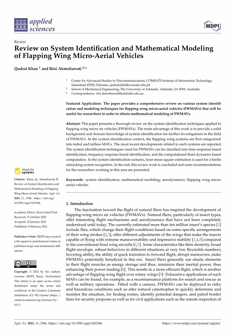
FWMAVs are primarily recognized and developed into two classes (i.e., tailless andtailed). The tailless designs usually mimic the insects, which, consequently, providehigh dynamic maneuvers. These configurations, in general, require active stabilizationbecause they can be found passively unstable in forward flight and hovering [22]. In suchdevelopments, the nano-hummingbird [7] and robotic bee, known as RoboBee [10], haveshown actual flight stability. On the other hand, the tailed design is found to be similarto configurations in birds, which are known for being passively stable, and thereforedo not require active stabilization [15,23]. This kind of configuration provides the easeto develop and implement higher-level problems like altitude stabilization [24,25] andobstacle avoidance [25–27]. Figure 1 displays some of the well-known flapping-wing microair vehicles that have been developed to date.

It is witnessed in Figure 1 that these FWMAVs differ in design as well as in its flyingmechanism. The FWMAVs (Figure 1a,b,f,h) follow very similar flight mechanics as birds.This class utilizes the surface control mechanism for different maneuvers like pitching,rolling, yawing, and hovering. The surface motion control resembles the fixed wing aircraftstrategies [7], whereas the FWMAVs in (Figure 1c,d,e,g) mimic the insects flying mech-anism to experience different flight maneuvers [11,14–16,19,20,28,29]. The autonomousflight of the first category is relatively easier compared to that of the second class of FW-MAVs. A clear understanding of insect flight depends on subtle details that might beeasily overlooked in otherwise thorough theoretical or experimental analyses. Recently,researchers have benefited greatly from the use of high-speed cameras for capturing wingkinematics, new strategies such as digital particle image velocimetry (DPIV) to quantifyflows, and powerful computers for further computational analysis. With the help of thesemethodologies, one can develop more accurate and rigorous models of these insects whilehaving a fewer number of assumptions in developing wing kinematics, aerodynamics, andflight dynamics.

Appl. Sci. 2021, 11, 1546 3 of 30Appl. Sci. 2021, 11, x FOR PEER REVIEW 3 of 30

Figure 1. (a) Festo-smartbird,manufactured by Festo’s Bionic Learning Network (photo courtesy of

Festo [14]); (b) AeroVironment Nano Hummingbird (photo courtesy of AeroVironment); (c) a

four-winged robot that flies with a jellyfish-like motion (photo courtesy of [16]); (d) DelFly MAV

(photo courtesy of Wikipedia-DelFly); (e) insect-scale flying robot (photo courtesy of Wyss Institute

Harvard University); (f) big bird developed by University of Maryland (Photo courtesy of Univer-

sity of Maryland); (g) Beetle Mimicking Flapping MAV (Photo courtesy of [11]); (h) Flapping wing

developed by Tamkang University (Photo courtesy of [29]).

Despite the challenges faced in conducting experiments to quantify the wing mo-

tions of several flying insects due to their small size and high wing beat frequencies, in-

sect fliers’ flapping kinematics, particularly that of free hovering flight and free forward

flight, have been well-researched for more than 50 years. Early attempts to capture

free-flight wing kinematics such as Ellington’s comprehensive and influential survey [30]

Figure 1. (a) Festo-smartbird, manufactured by Festo’s Bionic Learning Network (photo courtesyof Festo [14]); (b) AeroVironment Nano Hummingbird (photo courtesy of AeroVironment); (c) afour-winged robot that flies with a jellyfish-like motion (photo courtesy of [16]); (d) DelFly MAV(photo courtesy of Wikipedia-DelFly); (e) insect-scale flying robot (photo courtesy of Wyss InstituteHarvard University); (f) big bird developed by University of Maryland (Photo courtesy of Universityof Maryland); (g) Beetle Mimicking Flapping MAV (Photo courtesy of [11]); (h) Flapping wingdeveloped by Tamkang University (Photo courtesy of [29]).

Despite the challenges faced in conducting experiments to quantify the wing motionsof several flying insects due to their small size and high wing beat frequencies, insect fliers’flapping kinematics, particularly that of free hovering flight and free forward flight, have

Appl. Sci. 2021, 11, 1546 4 of 30

been well-researched for more than 50 years. Early attempts to capture free-flight wingkinematics such as Ellington’s comprehensive and influential survey [30] relied primarilyon a single-image high-speed cine. Although quite informative, especially because digitalimaging technology continues to offer exceptional spatial resolution, single-view techniquescannot provide an accurate time course of the angle of attack of the wings. More recentmethods have employed high-speed videography [31], which offers greater light sensitivityand ease of use, albeit at the cost of image resolution. A further consideration is that insectsrely extensively on visual feedback, and hence, care must be taken to ensure that lightingconditions do not significantly impair an insect’s behavior. Even more challenging thancapturing wing motions in 3-D is measuring the time course of aerodynamic forces duringthe stroke. At best, flight forces have been measured on the body of the insect rather thanits wings, making it very difficult to separate the inertial forces from the aerodynamic forcesgenerated by each wing [32–36]. In addition, unlike in free flight conditions, tethering canalter the wing motion, and thus, modify the generated forces. Researchers have overcomethese limitations using two strategies. The first method involves constructing dynamicallyscaled models on which it is easier to directly measure aerodynamic forces and visualizeflows [37–43]. A second approach is to construct computational fluid dynamic simulationsof flapping wings [44–48]. The power of both approaches, however, depends critically onaccurate knowledge of wing kinematics.

In general, to understand the mechanics of flapping wing flight, three basic aspectsneed to be well understood: flapping kinematics, aerodynamics, and flight dynamics (adetailed summary can be found in [49–51]). Several attempts have been made to modelFWMAVs based on the knowledge of those three aspects of natural fliers such as thosein [52], which focused on the first principle approach of modeling that includes flightstability and control. However, since FWMAVs depend on the flapping mechanism, theactuation system for generating the aerodynamic forces and moments as well as thesensors and control dynamics, mathematical models of FWMAVs solely based on the firstprinciples may not accurately describe the actual dynamics of the MAVs. The reviewprovided in this paper is intended to give insights into system identification approachesas an alternative way in obtaining mathematical models of various FWMAVs based onexperimental data. Such approaches differ from the conventional modeling approachesthrough physics (i.e., modeling through the first principles). With system identificationapproaches, the richness of experimental or flight data can be exploited to obtain the flightdynamics and aerodynamics characteristics of FWMAVs. The models obtained throughsuch approaches can be used to validate mathematical models (including those obtainedthrough the first principles) and predict the effect of any design changes.

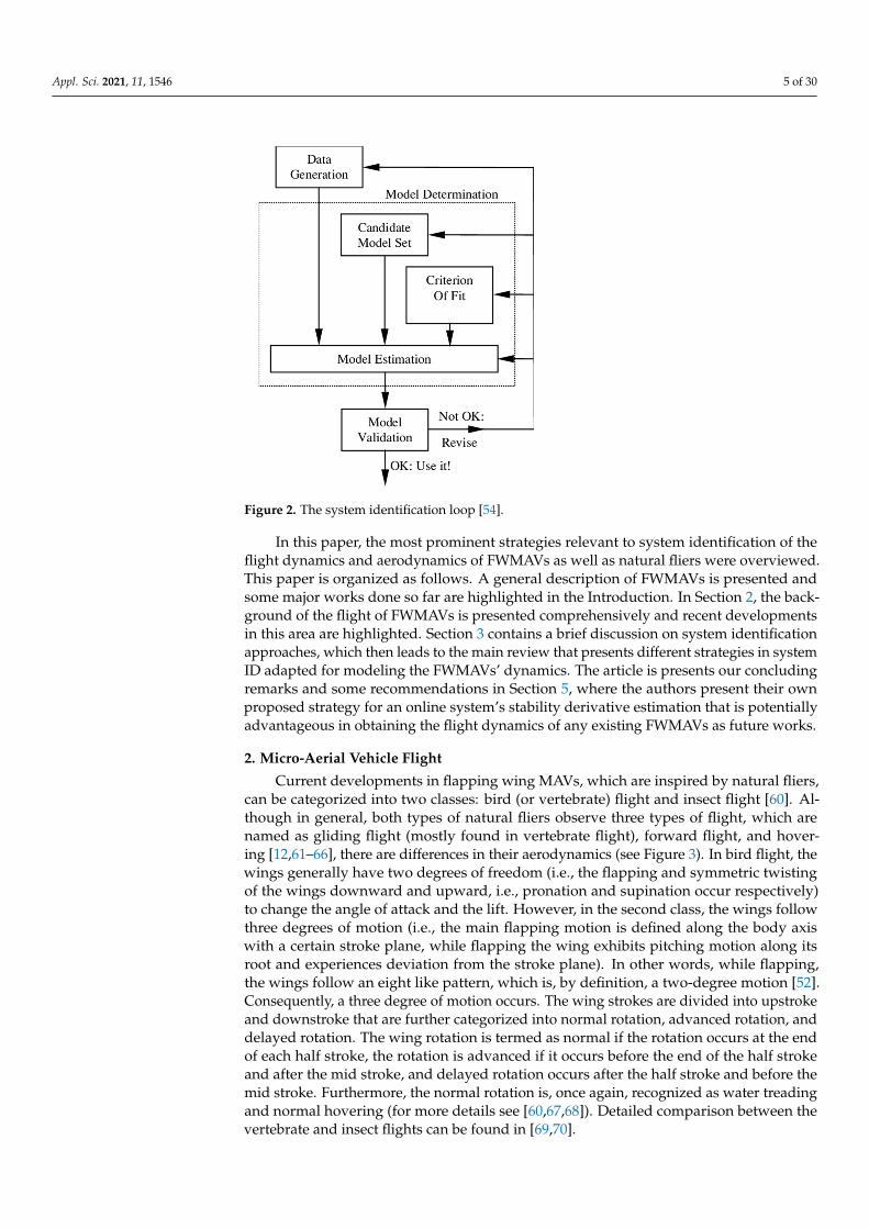
System identification uses mathematical modeling techniques, which are based onobserved input–output data. This process was first coined by Lofti Zadeh in the late1950s [53]. It has been used successfully to identify models of various complex systemssuch as the cardiovascular system [54], aircraft [55,56], and underwater vehicles [57]. Thistype of modeling approach is beneficial in developing realistic mathematical models ofcomplex systems based on experimental data for prediction, simulation, system design,and/or control [58]. System identification is usually conducted via (1) the Black boxapproach in which system identification is carried out by fitting the system’s input–outputresponse with some flight data, or (2) the Grey box approach (see [59] for more details),which is carried out by first developing the structure of models mathematically, thenthe required parameters in the models are identified. In both approaches, the overallmodels are validated against the experimental data. The typical steps involved in systemidentification are shown in Figure 2.

Appl. Sci. 2021, 11, 1546 5 of 30Appl. Sci. 2021, 11, x FOR PEER REVIEW 5 of 30

Figure 2. The system identification loop [54].

In this paper, the most prominent strategies relevant to system identification of the

flight dynamics and aerodynamics of FWMAVs as well as natural fliers were over-

viewed. This paper is organized as follows. A general description of FWMAVs is pre-

sented and some major works done so far are highlighted in the Introduction. In Section

2, the background of the flight of FWMAVs is presented comprehensively and recent

developments in this area are highlighted. Section 3 contains a brief discussion on system

identification approaches, which then leads to the main review that presents different

strategies in system ID adapted for modeling the FWMAVs’ dynamics. The article is

presents our concluding remarks and some recommendations in Section 5, where the

authors present their own proposed strategy for an online system’s stability derivative

estimation that is potentially advantageous in obtaining the flight dynamics of any ex-

isting FWMAVs as future works.

2. Micro-Aerial Vehicle Flight

Current developments in flapping wing MAVs, which are inspired by natural fliers,

can be categorized into two classes: bird (or vertebrate) flight and insect flight [60]. Alt-

hough in general, both types of natural fliers observe three types of flight, which are

named as gliding flight (mostly found in vertebrate flight), forward flight, and hovering

[12,61–66], there are differences in their aerodynamics (see Figure 3). In bird flight, the

wings generally have two degrees of freedom (i.e., the flapping and symmetric twisting

of the wings downward and upward, i.e., pronation and supination occur respectively)

to change the angle of attack and the lift. However, in the second class, the wings follow

three degrees of motion (i.e., the main flapping motion is defined along the body axis

with a certain stroke plane, while flapping the wing exhibits pitching motion along its

root and experiences deviation from the stroke plane). In other words, while flapping, the

wings follow an eight like pattern, which is, by definition, a two-degree motion [52].

Consequently, a three degree of motion occurs. The wing strokes are divided into up-

stroke and downstroke that are further categorized into normal rotation, advanced rota-

tion, and delayed rotation. The wing rotation is termed as normal if the rotation occurs at

the end of each half stroke, the rotation is advanced if it occurs before the end of the half

stroke and after the mid stroke, and delayed rotation occurs after the half stroke and be-

fore the mid stroke. Furthermore, the normal rotation is, once again, recognized as water

Figure 2. The system identification loop [54].

In this paper, the most prominent strategies relevant to system identification of theflight dynamics and aerodynamics of FWMAVs as well as natural fliers were overviewed.This paper is organized as follows. A general description of FWMAVs is presented andsome major works done so far are highlighted in the Introduction. In Section 2, the back-ground of the flight of FWMAVs is presented comprehensively and recent developmentsin this area are highlighted. Section 3 contains a brief discussion on system identificationapproaches, which then leads to the main review that presents different strategies in systemID adapted for modeling the FWMAVs’ dynamics. The article is presents our concludingremarks and some recommendations in Section 5, where the authors present their ownproposed strategy for an online system’s stability derivative estimation that is potentiallyadvantageous in obtaining the flight dynamics of any existing FWMAVs as future works.

2. Micro-Aerial Vehicle Flight

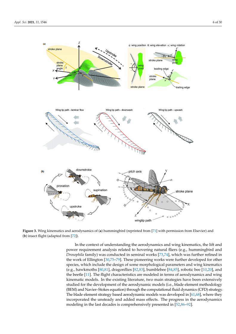
Current developments in flapping wing MAVs, which are inspired by natural fliers,can be categorized into two classes: bird (or vertebrate) flight and insect flight [60]. Al-though in general, both types of natural fliers observe three types of flight, which arenamed as gliding flight (mostly found in vertebrate flight), forward flight, and hover-ing [12,61–66], there are differences in their aerodynamics (see Figure 3). In bird flight, thewings generally have two degrees of freedom (i.e., the flapping and symmetric twistingof the wings downward and upward, i.e., pronation and supination occur respectively)to change the angle of attack and the lift. However, in the second class, the wings followthree degrees of motion (i.e., the main flapping motion is defined along the body axiswith a certain stroke plane, while flapping the wing exhibits pitching motion along itsroot and experiences deviation from the stroke plane). In other words, while flapping,the wings follow an eight like pattern, which is, by definition, a two-degree motion [52].Consequently, a three degree of motion occurs. The wing strokes are divided into upstrokeand downstroke that are further categorized into normal rotation, advanced rotation, anddelayed rotation. The wing rotation is termed as normal if the rotation occurs at the endof each half stroke, the rotation is advanced if it occurs before the end of the half strokeand after the mid stroke, and delayed rotation occurs after the half stroke and before themid stroke. Furthermore, the normal rotation is, once again, recognized as water treadingand normal hovering (for more details see [60,67,68]). Detailed comparison between thevertebrate and insect flights can be found in [69,70].

Appl. Sci. 2021, 11, 1546 6 of 30

Appl. Sci. 2021, 11, x FOR PEER REVIEW  6  of  30  

normal hovering (for more details see [60], [67], [68]). Detailed comparison between the 

vertebrate and insect flights can be found in [69] and [70]. 

Figure 3. Wing kinematics and aerodynamics of (a) hummingbird (reprinted from [71] with permission from Elsevier) and 

(b) insect flight (adapted from [72]). 

In the context of understanding the aerodynamics and wing kinematics, the lift and 

power  requirement analysis  related  to hovering natural  fliers  (e.g., hummingbird and 

Drosophila family) was conducted in seminal works [73,74], which was further refined in 

the work of Ellington  [30, 75–79]. These pioneering works were  further developed  for 

other species, which include the design of some morphological parameters and wing kin‐

ematics  (e.g.,  hawkmoths  [80,81],  dragonflies  [82,83],  bumblebee  [84,85],  robotic  bee 

[10,20], and the beetle [11]. The flight characteristics are modeled in terms of aerodynamics 

and wing kinematic models. In the existing literature, two main strategies have been ex‐

tensively  studied  for  the development of  the aerodynamic models  (i.e., blade  element 

Figure 3. Wing kinematics and aerodynamics of (a) hummingbird (reprinted from [71] with permission from Elsevier) and(b) insect flight (adapted from [72]).

In the context of understanding the aerodynamics and wing kinematics, the lift andpower requirement analysis related to hovering natural fliers (e.g., hummingbird andDrosophila family) was conducted in seminal works [73,74], which was further refined inthe work of Ellington [30,75–79]. These pioneering works were further developed for otherspecies, which include the design of some morphological parameters and wing kinematics(e.g., hawkmoths [80,81], dragonflies [82,83], bumblebee [84,85], robotic bee [10,20], andthe beetle [11]. The flight characteristics are modeled in terms of aerodynamics and wingkinematic models. In the existing literature, two main strategies have been extensivelystudied for the development of the aerodynamic models (i.e., blade element methodology(BEM) and Navier–Stokes equation) through the computational fluid dynamics (CFD) strategy.The blade element strategy based aerodynamic models was developed in [61,68], where theyincorporated the unsteady and added mass effects. The progress in the aerodynamicsmodeling in the last decades is comprehensively presented in [52,86–92].

Appl. Sci. 2021, 11, 1546 7 of 30

In recent developments, [93,94] tried to abridge the theoretical and experimentalstrategies and to develop a standard linear aerodynamic model for DelFly II. The devel-opments were mainly based on the standard aircraft system identification techniques andtheir extension to FWMAVs, which can be further used for simulation and autonomousfull flight envelope. In [95,96], a two-dimensional flapping wing was considered, andthe aerodynamic performance in asymmetric stroke in hovering and forward flight wasnumerically studied. In addition, the analysis of the effects of the asymmetry of the strokeon the aerodynamic forces and flow structures was carried out. The authors in [97] carriedout a BEM for the development of the fluid–structure interaction model by synthesizingit with a structural model. The benefits of this strategy were that it not only improvedthe reliability of the BEM, but it also enabled various aerodynamic studies (e.g., [98–102]).Note that the BEM method is widely utilized due to its simplicity and robustness, however,its accuracy has been questioned. In contrast, computational simulations based on thesolution of Navier–Stokes equations [103–105] have been utilized because they provide,with relatively high accuracy and precision, the detailed flow structures, time-dependentaerodynamic forces, and power requirements. However, this strategy needs high-fidelitymodeling and a long experiment processing time, which in turn diminishes its usagein practice.

A CFD-informed quasi-steady model based on a hybrid of high- and low-fidelity modelsto reduce the aforementioned complexity was presented in [106]. The systematic developmentregarding the beetle’s and DelFly II’s aerodynamics can be found in [107–109], respectively.In order to update the research carried out in the area of FWMAVs, a comprehensive biblio-metric review can be found in [110]. The flight stability of different species of natural fliers,particularly the longitudinal stability, was studied successfully by a number of researchers,for example, the stability of desert locust Schistocerca Gregaria was thoroughly presentedin [86], the nano-humming bird was focused on in [12], insects mimicking the FWMAV’sinitial stability was addressed in [111], and bumblebee stability was presented in [112]. Ingeneral, the eigenvalue-based analysis resulted in three modes common to all fliers, namely,the unstable oscillatory mode, stable fast subsidence mode, and stable slow subsidencemode. Almost all mathematical models developed in the aforementioned studies fall inthe category of modeling by the first principles. System identification approaches havehardly been used. Therefore, the forthcoming section will present, in detail, the techniquesdevised for system identification approaches, particularly, in obtaining system stabilityderivatives and control-oriented dynamic models of FWMAVs and natural flapping fliers.

3. System Identification and Mathematical Modeling of Flapping Wing Micro AirVehicles (FWMAVs)

The ultimate objective, in the development of FWMAVs, is securing an autonomousflight in order to utilize them for the different tasks mentioned earlier. Therefore, a firststep toward the establishment of an autonomous flight is the modeling of the flappingkinematics, aerodynamics, and flight dynamics of FWMAVs. This task is particularlychallenging due to inherent instability, nonlinear, time-varying, and periodic nature ofthe vehicles’ dynamics, especially during dynamic aerial maneuvers such as sharp andabrupt turns, obstacle avoidance, and mid-air prey capturing. The aerodynamics andflight dynamics of such maneuvers, even for natural fliers, have not been fully uncoveredyet. Additionally, on-board sensors, flapping mechanism, and actuation systems may addcomplexities to the overall dynamics of the MAVs. Furthermore, for insect-mimickingFWMAVs, due to their small size, the selection of hardware for their avionics and flightcontrol systems are limited. However, in this review, we focused on system identificationapproaches in order to model the FWMAVs without actually going through the details onhardware selection.

In general, two complementary strategies are applied to model FWMAVs. Thesestrategies are named as bottom-up and top-down [94]. The bottom-up approach mainlyfocuses on the fundamental approaches to explain and model the behavior and interactionof air motion with the flapping wings. This is essentially modeling with the first principles

Appl. Sci. 2021, 11, 1546 8 of 30

based on the well-studied aerodynamics and wing kinematics of natural flapping fliers(see [50] for a detailed summary). The practical system development of bio-inspiredFWMAVs remains the later part in such developments. On the other hand, in the top-downapproach, the construction and developments of the real MAVs take place prior to thetheoretical developments. In order to obtain the mathematical model(s) of the FWMAVs,the first step is the system identification, which means a strategy for acquiring a knownmathematical model (for instance, aerodynamic modeling, system stability derivatives,and system’s control derivatives) of the system while utilizing the available measured dataof the system’s input and output signals produced by the MAVs. These available signalsmay be measured either in time domain or in frequency domain. The main advantages ofperforming system identification in modeling are that the process uses real-time data andcan take into account design changes. The latter is particularly useful for control systemdesign. Through the process, the value of specific design parameters and their effects onthe dynamics of MAVs can be determined, and the structure of the mathematical modelsobtained is not unique, which gives the freedom to the engineers/researchers to selectthe models that suit the objectives of the modeling. For examples, these models may besuitable for (hardware-in-the-loop) simulations, analysis, and/or control.

With regard to this stage, the FWMAVs and their flight have been enlightened in ageneral way, and now the objective is to present the system identification in detail. It isgenerally conducted either for equivalent linear systems or core nonlinear systems. Thismay further be classified into time-domain and frequency-domain based identificationfor tailed and tailless FWMAVs. It is obvious that the dynamic modeling of FWMAVsalways considers the mechanism kinematics of linkages, which connect the motors andactuators to FWs [113], aerodynamic forces [114], and nonlinear phenomena like saturationand hysteresis [115]. Consequently, it results in different equations and realizations ofthe dynamics.

The linear modeling and identification of fixed wing aircraft were extensively studiedin [55,114]. The identification strategies for modeling FWMAVs or natural fliers vary fromsystem to system because of their varying kinematics and flight dynamics. The reviewpaper by [52] highlighted that the inertia effects of the wings on the main body wereinvoked in very few models of the flapping wing systems. The majority of the flappingangles of FWs remains greater than 20 degrees (see, for instance, [116]). Therefore, the smallangle assumption (i.e., sin(θ) ≈ θ) is no longer valid, and consequently, the linearizeddynamic model becomes inaccurate. The dynamic models of the FWs are generally highlynonlinear and time varying due to the aerodynamic forces on the wings that are typicallypredicted via the lift and drag coefficients of the quasi-steady aerodynamic model. Thesecoefficients depend on the angle of attack, which may vary significantly during a singlestroke. Various nonlinear modeling approaches have focused on the addition of a spring inthe redesign and optimization of the elastic elements like actuators, wings, and linkages tofurther improve the capability of the system to be driven at resonances [16–19]. Anotherstrategy [20] considered wing, actuator, and transmission components, and developed anintegrated nonlinear model, which considers all the changes made in the wing shape andlinkage system. The change in the wing shape significantly affects the inertial propertiesand the aerodynamic damping forces, whereas the variation in the linkage mechanismaffects the control input channels. Some useful linear models have also been developedthat account for the nonlinear geometric and aerodynamic components [117,118]. Thedeveloped nonlinear model sufficiently predicts the behavior of the FWMAVs with aconsiderable operating range. However, the accuracy in the model reduces when operatedat high frequencies.

The FWMAVs, as mentioned earlier, mimic either insect or bird flight. They are stabilizedvia active and passive stabilization strategies in different flight envelopes [10,12,30–32] throughmanually tuned controllers such as proportional-derivative (PD) and/or proportional-integral-derivative (PID) controllers. However, they are observed to be sensitive to externaldisturbances. Thus, it becomes quite challenging to keep them stable in broad flight envelopes.

Appl. Sci. 2021, 11, 1546 9 of 30

One reason for such difficulties is the absence of a sufficiently accurate nonlinear modelthat can describe the unsteady aerodynamics of the FWMAVs’ flapping motions [119,120]and the added inertia effect contribution to the MAVs dynamics [121]. In this context,a linear time invariant (LTI) model was developed in [121–124] via the use of standardaircraft equations. Another approach, known as the multi-body approach, was introduced.However, such an approach for a time varying nonlinear model [121,125] is not suitablefor onboard processing. All the aforementioned approaches have significant shortcomingssuch as a lack of practical validation, limited only to computational environment and therepeatability of the data. Therefore, it is demanding to overcome such modeling difficultiesin order to fully explore the capabilities of these fliers.

In the subsequent subsections, we will focus on system identification strategies thathave been applied for identifying parameters and mathematical models of FWMAVs. Inpresenting the review, we classify natural fliers and FWMAVs into two categories, the tailedand tailless fliers/FWMAVs. Various system identification techniques used in identifyingthe model parameters of fliers/FWMAVs in these two categories will be discussed.

3.1. Tailed Flapping Wing Micro-Air Vehicles

In this section, we intend to present the details of system identification techniquesfor tailed micro air vehicles (i.e., bird like micro air vehicles). In [126,127], a flight testof a 0.45 kg ornithopter was flown in a straight and level mean flight. A visual trackingstrategy was employed to provide measurements of the states, which benefited with low-noise, minimally-invasive measurements. The spatial distributions of kinematics over awing stroke were investigated while using a multi-body model of the flight dynamics.The models of lift, thrust, and the coefficients of pitching moment were extracted viastepwise regression accompanied by least mean square estimation. Both the frequencyand time domain system identification strategies were invoked, which resulted in quiteclose estimates. The identified models can be used for feedback control purposes. A greybox approach was proposed for the system identification of the DelFly II in [93,94,128],which by definition belongs to the top-down approach. The purpose of their work was tobridge the existing gap between the theoretical and experimental strategies. Another coreobjective was the development of benchmark aerodynamic models for the DelFly II basedon aircraft system identification techniques. In addition, the extension of these techniquesto the flapping wing system for autonomous flight was the key objective. The identificationwas mainly done via the least mean square estimation and extended Kalman filter (EKF),which are highlighted in the subsequent study.

3.1.1. System Identification of DelFly II Based on Least Mean Square Estimation

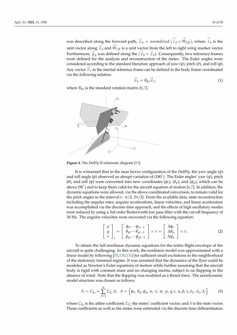
The Delfly II, shown in Figure 4, is a bioinspired ornithopter, which is configuredwith four flapping wings and an inverted ‘T’ tail. Its weight is 17 g and is capable ofhovering flight as well as forward flight at the speed of 8 ms−1 [93]. The experimentalflight was conducted in an experimental chamber, which was equipped with a trackingsystem capable of recording the position of a small reflective marker at 200 Hz frequency.The position and altitude were tracked via the use of eight markers placed on its structure.A set of longitudinal elevator input with step, doublets, and triplets with a reference timeof 0.3 s was programmed into its autopilot to acquire a full dynamic response over a set offrequencies. The framework for the system identification was defined as follows. The firststep toward the system identification was observation/estimation of the state variablesof the system from the provided position data. This process was named as flight pathreconstruction in [129]. Then, these estimated and available data were used to reconstructthe indirectly measurable states such as angle of attack and refinement of the estimatedstates. The whole reconstruction was carried out in two reference frames. The trackingsystem frame was named as the inertial reference frame and was indicated with a subscript

I at the respective coordinate axes so that the positive→Z I was pointing upward. The frame

fixed with body was identified by a subscript b at the respective frame. The positive→x b

Appl. Sci. 2021, 11, 1546 10 of 30

was described along the forward path,→z b = normalized (

→i b ×

→WLR), where

→i b is the

unit vector along→x b and

→WLR is a unit vector from the left to right wing marker vector.

Furthermore,→y b was defined along the (

→x b ×

→z b). Consequently, two reference frames

were defined for the analysis and reconstruction of the states. The Euler angles wereconsidered according to the standard literature approach of yaw (ψ), pitch (θ), and roll (φ).Any vector

→v I in the inertial reference frame can be defined in the body frame coordinated

via the following relation.→v b = RbI

→v I , (1)

where RbI is the standard rotation matrix [6,7].

Appl. Sci. 2021, 11, x FOR PEER REVIEW  10  of  30  

conducted in an experimental chamber, which was equipped with a tracking system ca‐

pable of recording the position of a small reflective marker at 200 Hz frequency. The po‐

sition and altitude were tracked via the use of eight markers placed on its structure. A set 

of longitudinal elevator input with step, doublets, and triplets with a reference time of 0.3 

s was programmed into its autopilot to acquire a full dynamic response over a set of fre‐

quencies. The framework for the system identification was defined as follows. The first 

step toward the system identification was observation/estimation of the state variables of 

the system from the provided position data. This process was named as flight path recon‐

struction in [129]. Then, these estimated and available data were used to reconstruct the 

indirectly measurable states such as angle of attack and refinement of the estimated states. 

The whole reconstruction was carried out in two reference frames. The tracking system 

frame was named as the inertial reference frame and was indicated with a subscript I at 

the respective coordinate axes so  that  the positive  𝑍 was pointing upward. The  frame 

fixed with body was identified by a subscript b at the respective frame. The positive  ��  was described along the forward path,  𝑧 𝑛𝑜𝑟𝑚𝑎𝑙𝑖𝑧𝑒𝑑 𝚤 �� , where  𝚤   is the unit vector along  �� and  �� is a unit vector from the left to right wing marker vector. Fur‐

thermore,  �� was defined along the  �� 𝑧 ). Consequently, two reference frames were 

defined for the analysis and reconstruction of the states. The Euler angles were considered 

according to the standard literature approach of yaw (ψ), pitch (θ), and roll (ϕ). Any vec‐

tor  �� in the inertial reference frame can be defined in the body frame coordinated via the 

following relation. 

�� 𝑅 �� ,  (1)

where  𝑅   is the standard rotation matrix [6,7]. 

Figure 4. The DelFly II schematic diagram [93]. 

It is witnessed that in the near hover configuration of the DelFly, the yaw angle (ψ) 

and roll angle (ϕ) observed an abrupt variation of (180°). The Euler angles’ yaw (ψ), pitch 

(θ), and roll (ϕ) were converted into new coordinates (𝜙 ), (𝜃 ), and (𝜓 ), which can be 

above (90°) and to keep them valid for the aircraft equation of motion [6,7]. In addition, 

the dynamic equations were allowed, via  the above coordinated conversion,  to remain 

valid for the pitch angles in the interval (‐π/2,3π/2). From the available data, state recon‐

struction  including the angular rates, angular accelerations, linear velocities, and  linear 

acceleration was accomplished via the discrete time approach, and the effects of high os‐

cillatory modes were reduced by using a 3rd order Butterworth  low pass filter with the 

cut‐off frequency of 30 Hz. The angular velocities were recovered via the following equa‐

tion: 

Figure 4. The DelFly II schematic diagram [93].

It is witnessed that in the near hover configuration of the DelFly, the yaw angle (ψ)and roll angle (φ) observed an abrupt variation of (180

◦). The Euler angles’ yaw (ψ), pitch

(θ), and roll (φ) were converted into new coordinates (φr), (θp), and (ψy), which can beabove (90

◦) and to keep them valid for the aircraft equation of motion [6,7]. In addition, the

dynamic equations were allowed, via the above coordinated conversion, to remain valid forthe pitch angles in the interval (−π/2, 3π/2). From the available data, state reconstructionincluding the angular rates, angular accelerations, linear velocities, and linear accelerationwas accomplished via the discrete time approach, and the effects of high oscillatory modeswere reduced by using a 3rd order Butterworth low pass filter with the cut-off frequency of30 Hz. The angular velocities were recovered via the following equation: p

qr

t

=

φrt − φrt−1θpt − θpt−1ψyt − ψyt−1

× τ =

∆φr∆θp∆ψy

× τ. (2)

To obtain the full nonlinear dynamic equations for the entire flight envelope of theaircraft is quite challenging. In this work, the nonlinear model was approximated with alinear model by following [55,130,131] for sufficient small excitations in the neighborhoodof the stationary trimmed regime. It was assumed that the dynamics of the flyer could bemodeled as Newton’s Euler equations of motion while further assuming that the aircraftbody is rigid with constant mass and no changing inertia, subject to no flapping in theabsence of wind. Note that the flapping was modeled as a thrust force. The aerodynamicmodel structure was chosen as follows:

Fi = CF0 +n

∑S=1

CFs .S; S ={

φr, θp, ψy, u, v, w, p, q, r, α, β, γ, δ f , δe, δr

}(3)

where CF0 is the affine coefficient; CFs the states’ coefficient vector; and S is the state vector.These coefficients as well as the states were estimated via the discrete time differentiation.

Appl. Sci. 2021, 11, 1546 11 of 30

Equation (3) represents the full model structure so that the aerodynamic forces and mo-ments are expressed as linear functions of states. The reduced model is expressed in aform, which only needs the measurable available states. The core objective of the reducedmodel was to use it in the flight controller design. The reduced model structure appearsas follows:

X = X0 + Xqq + Xθθ + Xδe δe + Xδ f δ f , Y = Y0 + YPP + Yφφ + Yδr δr + Yδ f δ f ,Z = Z0 + Zqq + Zθθ + Zδe δe + Zδ f δ f , L = L0 + Lθθ + Lδr δr + lδ f δ f ,M = M0 + Mθθ + Mδe δe + Mδ f δ f , N = N0 + Nθθ + Nδr δr + Nδ f δ f .

(4)

The parameter estimation was carried out via the conventional least square estimator.The parameter estimation of the aforesaid forces and moments can be recovered, forexample, as follows:

X0XqXθ

Xδe

Xδ f

=(

RT R)−1

RTX, R =

1 q(1) θ(1) δe(1) δ f (1)1 q(2) θ(2) δe(2) δ f (2)...

......

......

1 q(N) θ(N) δe(N) δ f (N)

(5)

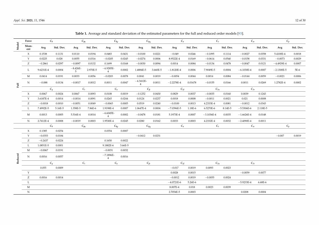
where R is the regression matrix with N observations. The input profile on the elevatorto conduct five longitudinal flight maneuvers in the near hover and slow forward flightscenarios included step, doublet, and triplet commands. The parameters were estimatedfor different flight scenarios. The proximity in the estimated parameter was helpful inchoosing a single model for the control design purpose. The estimated parameters aredisplayed in Table 1 [93].

The model validation was also conducted via two different strategies. In the firstmethod, the validation of the maneuvers was done. In this case, the estimated parametersin the identification cycle were utilized to forecast the aerodynamic forces and moments ofother maneuvers. On the other hand, in the second scenario, the validation was done viasimulations. In this case, the estimated parameters were used in the nonlinear dynamicsimulator, then the states and flight path were reconstructed and compared with the actualflight test data.

The system identification and model validation were carried out via the Grey boxmethod and the parameters were estimated for two different dynamic models, which werenamed as full order and reduced order for different flight regimes. It was concluded that thedeveloped models were successfully obtained. However, further study is still required toachieve the prediction of the aerodynamic forces and moments with considerable accuracyfor a longer period of time and full autonomous flight missions. In this regard, veryappealing developments have been reported in [132,133].

Appl. Sci. 2021, 11, 1546 12 of 30

Table 1. Average and standard deviation of the estimated parameters for the full and reduced order models [93].

Mod

el

Force C0 Cφr Cθp Cψy Cu Cv Cw Cp

Mom-ent Avg Std. Dev. Avg Std. Dev. Avg Std. Dev. Avg Std. Dev. Avg Std. Dev. Avg Std. Dev. Avg Std. Dev. Avg Std. Dev.

Full

X 0.1538 0.1131 0.0110 0.0194 0.0483 0.0431 −0.0100 0.0221 −0.049 0.0246 −0.1095 0.1114 −0.0027 0.0358 5.4100E-4 0.0018

Y 0.0225 0.028 0.0055 0.0316 −0.0205 0.0245 −0.0274 0.0006 8.9522E-4 0.0169 −0.0614 0.0540 −0.0158 0.0331 −0.0073 0.0029

Z −0.2861 0.0297 −0.0097 0.0132 0.1699 0.0168 −0.0030 0.0094 0.0014 0.0084 −0.0134 0.0478 −0.0047 0.0121 −4.4929E-4 0.0007

L 9.6231E-4 0.0004 −8.426E-5 2.970E-5 −6.9285E-

4 0.0002 1.4884E-5 3.660E-5 −1.8120E-4 0.0006 7.9049E-5 0.0004 −6.1030E-4 0.0007 −2.1300E-5 5E-6

M 0.0414 0.0191 0.0033 0.0056 −0.0203 0.0078 0.0041 0.0019 −0.0054 0.0044 0.0014 0.0084 −0.0144 0.0059 −0.0021 0.0006

N −0.088 0.0134 −0.0017 0.0012 0.0011 0.0047 −4.3412E-4 0.0011 −2.2278E-4 0.01678 −0.0155 0.0166 0.0011 0.0269 1.2782E-4 0.0002

Cq Cr Cα Cβ Cδf Cδa Cδr

X 0.0067 0.0024 0.0067 0.0093 0.0108 0.0019 −0.1252 0.0430 0.0829 0.0037 −0.0035 0.0160 0.0039 0.1243

Y 3.6187E-4 0.0014 −0.0014 0.0091 0.0265 0.0244 0.0124 0.0237 0.0018 0.0008 −0.0011 0.0021 0.021 0.0008

Z −0.0018 0.0010 −0.0051 0.0049 −0.0065 0.0005 0.0519 0.0240 −0.0100 0.0013 4.2333E-4 0.0081 −0.0012 0.0343

L 7.4992E-5 5.16E-5 1.358E-5 7.86E-6 1.9198E-4 0.0007 1.0647E-4 0.0004 −7.0396E-5 1.18E-6 6.5270E-6 8.14E-5 −5.5306E-6 2.118E-5

M 0.0013 0.0005 5.516E-4 0.0014 −6.6045E-4 0.0002 −0.0478 0.0181 5.1973E-4 0.0007 −3.1036E-4 0.0035 −1.6626E-4 0.0148

N 2.7412E-4 0.0008 −0.0019 0.0003 1.9530E-4 0.0245 0.0280 0.0162 0.0033 0.0003 4.2332E-4 0.0032 −2.4090E-4 0.0011

C0 Cφr Cθp Cψy Cu Cv Cw Cp

Red

uced

X 0.1385 0.0254 0.0354 0.0007

Y −0.0353 0.0184 −0.0412 0.0231 −0.007 0.0019

Z −0.2437 0.0224 0.1650 0.0022

L 1.0851E-5 0.0001 9.1882E-6 3.66E-5

M −0.0067 0.0191 −0.0031 0.0032

N 0.0016 0.0057 −7.1896E-4 0.0016

Cq Cr Cα Cβ . Cδf Cδa Cδr

0.055 0.0009 −0.017 0.0019 0.0093 0.0023

Y 0.0028 0.0015 −0.0059 0.0077

Z 0.0016 0.0014 −0.0012 0.0019 −0.0055 0.0024

L −4.0721E-6 5.26E-6 −5.9233E-4 6.68E-6

M 8.007E-4 0.018 0.0023 0.0039

N 2.7054E-5 0.0003 0.0208 0.0004

Appl. Sci. 2021, 11, 1546 13 of 30

3.1.2. System Identification of DelFly II Based on Extended Kalman Filter

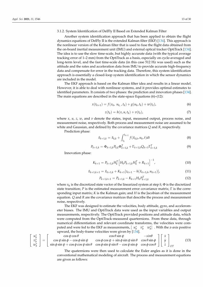
Another system identification approach that has been applied to obtain the flightdynamics equations of DelFly II is the extended Kalman filter (EKF) [134]. This approach isthe nonlinear version of the Kalman filter that is used to fuse the flight data obtained fromthe on-board inertial measurement unit (IMU) and external optical tracker OptiTrack [134].The idea is to use the slow time-scale, but highly accurate data (with the typical averagetracking error of 1–2 mm) from the OptiTrack as a basis, especially on cycle-averaged andlong-term level, and the fast time-scale data (in this case 512 Hz was used) such as theattitude and the rates and acceleration data from IMU to provide accurate high-frequencydata and compensate for error in the tracking data. Therefore, this system identificationapproach is essentially a closed-loop system identification in which the sensor dynamicsare included in the model.

The EKF approach is based on the Kalman filter idea and results in a linear model.However, it is able to deal with nonlinear systems, and it provides optimal estimates toidentified parameters. It consists of two phases: the prediction and innovation phases [134].The main equations are described in the state-space Equations (6)–(12):

x(tk+1) = f (xk, uk, , tk) + g(uk, tk) + w(tk), (6)

z(tk) = h(x, u, tk) + v(tk), (7)

where x, u, z, w, and v denote the states, input, measured output, process noise, andmeasurement noise, respectively. Both process and measurement noise are assumed to bewhite and Gaussian, and defined by the covariance matrices Q and R, respectively.

Prediction phase:

xk+1,k = xk,k +∫ tk+1

tk

f (xk,k, uk, t)dt (8)

Pk+1,k = Φk+1,kPk,kΦTk+1,k + Γk+1,kQk+1ΓT

k+1,k (9)

Innovation phase:

Kk+1 = Pk+1,k HTk

[HkPk+1,k HT

k + Rk+1

]−1, (10)

xk+1,k+1 = xk+1,k + Kk+1[zk+1 − h(xk+1,k, uk+1)], (11)

Pk+1,k+1 = Pk+1,k − Kk+1HkPTk+1,k (12)

where xk is the discretized state vector of the linearized system at step k; Φ is the discretizedstate transition; P is the estimated measurement error covariance matrix; Γ is the corre-sponding input matrix; K is the Kalman gain; and H is the Jacobian of the measurementequation. Q and R are the covariance matrices that describe the process and measurementnoise, respectively.

The EKF was designed to estimate the velocities, body attitude, gyro, and accelerom-eter biases. The IMU and OptiTrack data were used as the input variables and outputmeasurements, respectively. The OptiTrack provided positions and attitude data, whichwere computed from the OptiTrack-measured quarternions. From these data, throughnumerical differentiation and relevant coordinate transforms, the velocities were com-puted and were fed to the EKF as measurements, [ u∗b v∗b w∗b ] . With the z-axis positiveupward, the body-frame velocities were given by [134]. u∗b

v∗bw∗b

=

cos ψ cos θ cos θ sin ψ −sinθcos ψ sin φ− cos φ sin ψ cos φ cos ψ + sin φ sin ψ sin θ cos θ sin φ

sin φ sin ψ + cos φ cos ψ sin θ cos φ sin ψ sin θ − cos ψ sin φ cos φ cos θ

.x.y.z

OT

(13)

The quaternions were then used to calculate the Euler angles as it is done in theconventional mathematical modeling of aircraft. The process and measurement equationsare given as follows:

Appl. Sci. 2021, 11, 1546 14 of 30

Process equations:

.Φ = (p− bp) + (q− bq) sin Φ tan Θ + (r− br) cos Φ tan Θ.

Θ = (q− bq) cos Φ− (r− br) sin Φ.

Ψ = (q− bq) sin Φ sec Θ + (r− br) cos Φ sec Θ.uB = (r− br)vb − (q− bq)wb − g sin Θ + az − bax.vB = −(r− br)ub + (p− bp)wb + g sin Φ cos Θ + ay − bay.wB = (q− bq)ub − (p− bp)vb + g cos Φ cos Θ + az − baz.bP = 0.bq = 0.br = 0.bax = 0.bay = 0.baz = 0

Measurement equations:Φm = Φ + υΦΘm = Θ + υθ

Ψm = ψ + υΨu∗b = ub + υxv∗b = vb + υy

w∗b = wb + υz,

where x, u, z, v, and w are the states, input, output, process, and measurement noise termsof the filter, respectively, and are defined as follows.

x =[

Φ Θ Ψ ub vb wb bp bq br baz bay baz]T ,

u =[

p q r az ay ax]T ,

z =[

Φm Θm Ψm u∗b v∗b w∗b]T ,

υ =[

υΦ υΘ υΨ υub υvb υwb]T ,

w =[

wp wq wr wax way waz]T .

The states were the attitudes (i.e., the Euler angles [Φ Θ Ψ]), body-axis velocities[ub, vb, wb], and the sensor biases of the gyroscope and accelerometer

[bp, bq, br, bax, bay, baz

].

The input was the roll, pitch, and yaw rates [p, q, r] and the accelerometer-measuredaccelerations

[ax, ay, az

]. The output z were the attitude obtained from the OptiTrack

system and velocities. The process noise term v consisted of the measurement noise in themeasured velocities and attitudes. Finally, the measurement noise term w consisted of theprocess noise in the rates and accelerations.

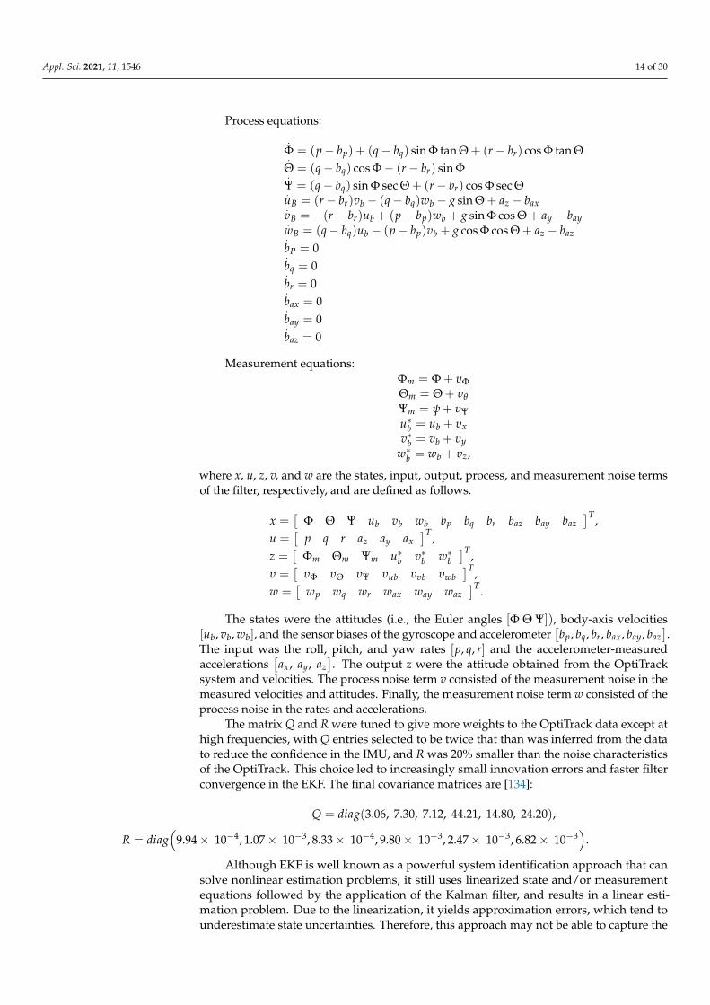
The matrix Q and R were tuned to give more weights to the OptiTrack data except athigh frequencies, with Q entries selected to be twice that than was inferred from the datato reduce the confidence in the IMU, and R was 20% smaller than the noise characteristicsof the OptiTrack. This choice led to increasingly small innovation errors and faster filterconvergence in the EKF. The final covariance matrices are [134]:

Q = diag(3.06, 7.30, 7.12, 44.21, 14.80, 24.20),

R = diag(

9.94× 10−4, 1.07× 10−3, 8.33× 10−4, 9.80× 10−3, 2.47× 10−3, 6.82× 10−3)

.

Although EKF is well known as a powerful system identification approach that cansolve nonlinear estimation problems, it still uses linearized state and/or measurementequations followed by the application of the Kalman filter, and results in a linear esti-mation problem. Due to the linearization, it yields approximation errors, which tend tounderestimate state uncertainties. Therefore, this approach may not be able to capture the

Appl. Sci. 2021, 11, 1546 15 of 30

nonlinearities and time-varying nature of the dynamics of FWMAVs accurately. This prob-lem can be improved by selecting process equations, which give better descriptions of thedynamics, and in this case, a priori knowledge and engineering insights will be required.

3.1.3. System Identification of Kinkade Slow Hawk Ornithopter

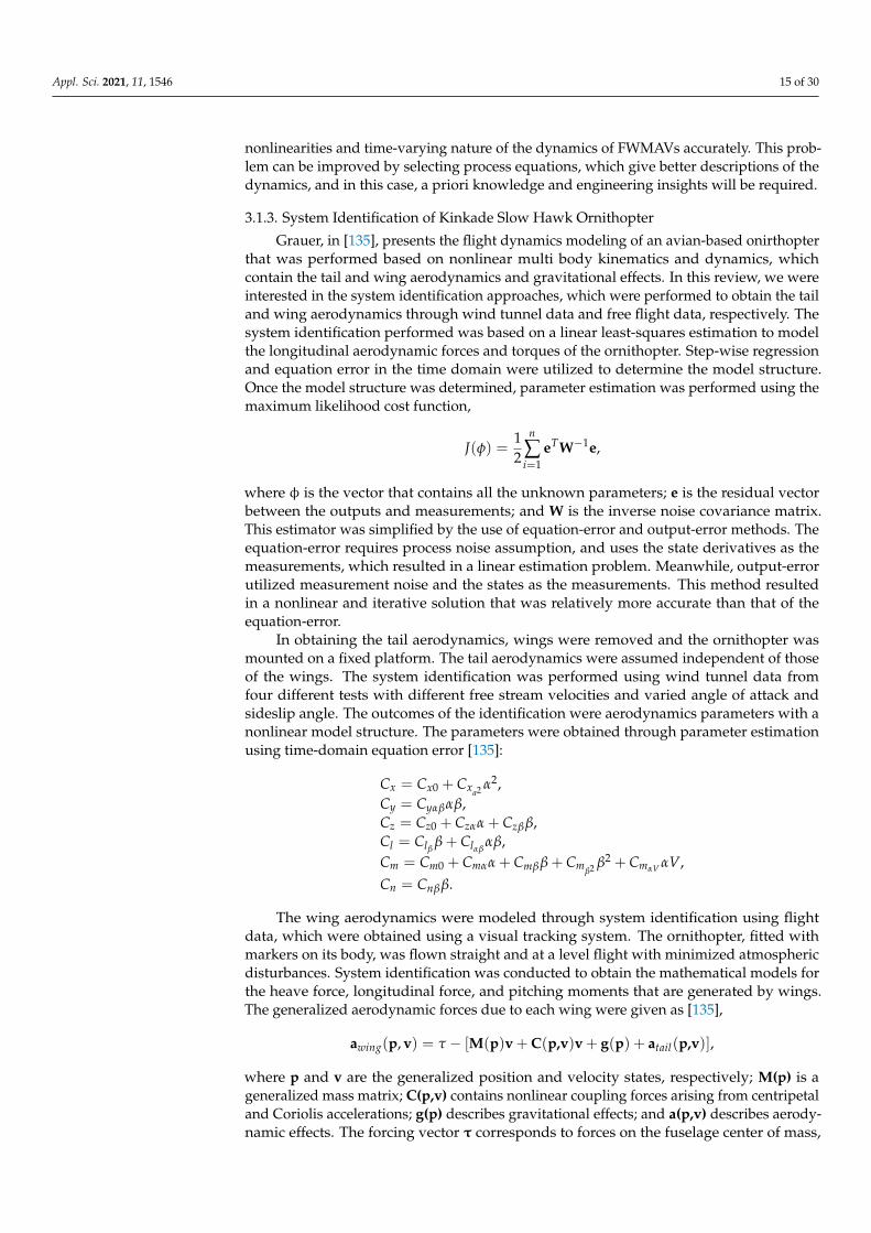
Grauer, in [135], presents the flight dynamics modeling of an avian-based onirthopterthat was performed based on nonlinear multi body kinematics and dynamics, whichcontain the tail and wing aerodynamics and gravitational effects. In this review, we wereinterested in the system identification approaches, which were performed to obtain the tailand wing aerodynamics through wind tunnel data and free flight data, respectively. Thesystem identification performed was based on a linear least-squares estimation to modelthe longitudinal aerodynamic forces and torques of the ornithopter. Step-wise regressionand equation error in the time domain were utilized to determine the model structure.Once the model structure was determined, parameter estimation was performed using themaximum likelihood cost function,

J(φ) =12

n

∑i=1

eTW−1e,

where φ is the vector that contains all the unknown parameters; e is the residual vectorbetween the outputs and measurements; and W is the inverse noise covariance matrix.This estimator was simplified by the use of equation-error and output-error methods. Theequation-error requires process noise assumption, and uses the state derivatives as themeasurements, which resulted in a linear estimation problem. Meanwhile, output-errorutilized measurement noise and the states as the measurements. This method resultedin a nonlinear and iterative solution that was relatively more accurate than that of theequation-error.

In obtaining the tail aerodynamics, wings were removed and the ornithopter wasmounted on a fixed platform. The tail aerodynamics were assumed independent of thoseof the wings. The system identification was performed using wind tunnel data fromfour different tests with different free stream velocities and varied angle of attack andsideslip angle. The outcomes of the identification were aerodynamics parameters with anonlinear model structure. The parameters were obtained through parameter estimationusing time-domain equation error [135]:

Cx = Cx0 + Cxa2 α2,Cy = Cyαβαβ,Cz = Cz0 + Czαα + Czββ,Cl = Clβ

β + Clαβαβ,

Cm = Cm0 + Cmαα + Cmββ + Cmβ2 β2 + CmαV αV,

Cn = Cnββ.

The wing aerodynamics were modeled through system identification using flightdata, which were obtained using a visual tracking system. The ornithopter, fitted withmarkers on its body, was flown straight and at a level flight with minimized atmosphericdisturbances. System identification was conducted to obtain the mathematical models forthe heave force, longitudinal force, and pitching moments that are generated by wings.The generalized aerodynamic forces due to each wing were given as [135],

awing(p, v) = τ − [M(p)v + C(p,v)v + g(p) + atail(p,v)],

where p and v are the generalized position and velocity states, respectively; M(p) is ageneralized mass matrix; C(p,v) contains nonlinear coupling forces arising from centripetaland Coriolis accelerations; g(p) describes gravitational effects; and a(p,v) describes aerody-namic effects. The forcing vector τ corresponds to forces on the fuselage center of mass,

Appl. Sci. 2021, 11, 1546 16 of 30

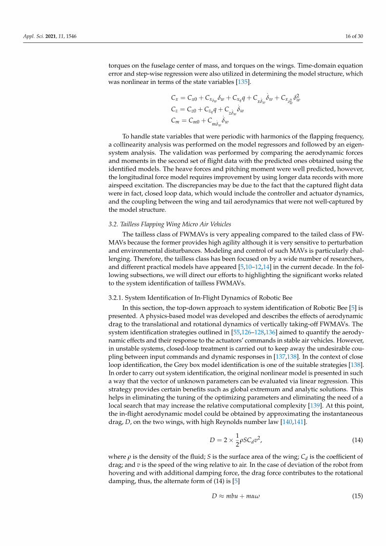
torques on the fuselage center of mass, and torques on the wings. Time-domain equationerror and step-wise regression were also utilized in determining the model structure, whichwas nonlinear in terms of the state variables [135].

Cx = Cx0 + Cxδwδw + Cxq q + C

x.δw

.δw + Cx

δ2w

δ2w

Cz = Cz0 + Czq q + Cz

.δw

.δw

Cm = Cm0 + Cm

.δw

.δw

To handle state variables that were periodic with harmonics of the flapping frequency,a collinearity analysis was performed on the model regressors and followed by an eigen-system analysis. The validation was performed by comparing the aerodynamic forcesand moments in the second set of flight data with the predicted ones obtained using theidentified models. The heave forces and pitching moment were well predicted, however,the longitudinal force model requires improvement by using longer data records with moreairspeed excitation. The discrepancies may be due to the fact that the captured flight datawere in fact, closed loop data, which would include the controller and actuator dynamics,and the coupling between the wing and tail aerodynamics that were not well-captured bythe model structure.

3.2. Tailless Flapping Wing Micro Air Vehicles

The tailless class of FWMAVs is very appealing compared to the tailed class of FW-MAVs because the former provides high agility although it is very sensitive to perturbationand environmental disturbances. Modeling and control of such MAVs is particularly chal-lenging. Therefore, the tailless class has been focused on by a wide number of researchers,and different practical models have appeared [5,10–12,14] in the current decade. In the fol-lowing subsections, we will direct our efforts to highlighting the significant works relatedto the system identification of tailless FWMAVs.

3.2.1. System Identification of In-Flight Dynamics of Robotic Bee

In this section, the top-down approach to system identification of Robotic Bee [5] ispresented. A physics-based model was developed and describes the effects of aerodynamicdrag to the translational and rotational dynamics of vertically taking-off FWMAVs. Thesystem identification strategies outlined in [55,126–128,136] aimed to quantify the aerody-namic effects and their response to the actuators’ commands in stable air vehicles. However,in unstable systems, closed-loop treatment is carried out to keep away the undesirable cou-pling between input commands and dynamic responses in [137,138]. In the context of closeloop identification, the Grey box model identification is one of the suitable strategies [138].In order to carry out system identification, the original nonlinear model is presented in sucha way that the vector of unknown parameters can be evaluated via linear regression. Thisstrategy provides certain benefits such as global extremum and analytic solutions. Thishelps in eliminating the tuning of the optimizing parameters and eliminating the need of alocal search that may increase the relative computational complexity [139]. At this point,the in-flight aerodynamic model could be obtained by approximating the instantaneousdrag, D, on the two wings, with high Reynolds number law [140,141].

D = 2× 12

ρSCdv2, (14)

where ρ is the density of the fluid; S is the surface area of the wing; Cd is the coefficient ofdrag; and v is the speed of the wing relative to air. In the case of deviation of the robot fromhovering and with additional damping force, the drag force contributes to the rotationaldamping, thus, the alternate form of (14) is [5]

D ≈ mbu + mαω (15)

Appl. Sci. 2021, 11, 1546 17 of 30

where m is the mass of the robot; b is the normalized drag force; u is the speed in forwarddirection; α is the angle of attack; and ω is the rotational speed of the robot.

The resulting drag moment can be expressed as follows:

M ≈ Jcω + Jβu, (16)

where c and β are the rotational damping coefficients normalized by inertia. Due to (15)and (16), the viscous forces and torque from the wings, which dominate the drag forcesand are shown critical to the open loop dynamics and stability of FWMAVs [34,141,142],can also be treated as linear functions.

The translational dynamic equation of the robot can be modeled as follows:

m..X = mΓZ + W + Fa, (17)

where Fa represents the lumped aerodynamic forces; W = mg represents the gravitationalforce; Γ is the normalized thrust with dimension of acceleration; and Z represents the axisalong the body of the robots. It includes the additional aerodynamic force due to dragforces on the wings and viscous forces on the body that can be further modeled as linearfunctions of translational and angular velocities. Equation (17), with explicit expression ofFa, can be re-expressed as follows:

ddt

.X + ω×

.X =

00Γ

− g

R31R32R32

+

−bx.x− αxωy

−by.y + αyωx−bz

.z

, (18)

where bi and αi are contributed from the body velocity and angular velocity with i ∈ {x, y,z}. When the FWMAV is not in perfect hovering, then it is affected by additional torques,therefore, the resultant torque on the robot can be expressed by the following rotationaldynamic equations:

∑ τ = Jdω

dt+ ω× Jω = τc + τa + Jd, (19)

where Jd is the unknown normalized disturbance. Note that in this presentation, the rolland pitch were focused and the aerodynamic contributions were modeled as linear in itsvariables. In more detail, this equation can be expressed as follows:

ddt

[ωxωy

]=

[τc, x J−1

xτc, y J−1

y

]+

[ (Jy − Jz

)J−1x 0

0 (Jz − Jx)J−1y

][ωxωzωyωz

]+

[−cxωx + βx

.y

−cyωy − βy.x

]+

[dxdy

]. (20)

The aforementioned Equations (18) and (20) are linear in their structures and therefore,the estimation of unknown parameters via the linear regression approach is the ultimateobjective. The linear regression model could be expressed as follows:

Ψi = ϕ0 + ∑nj=1χij ϕj + εi; i ∈ {1, 2, . . . , N}, (21)

where ϕ0 represents an unknown possible offset or affine term; εi represents the residualof an ith observation; N is the number of total observations; n is the number of unknownparameters; and Ψ is an N × 1 vector, which needs to be extracted. The following leastsquare estimator is considered to provide the estimated parameters.

ϕ = (χTχ)−1

χTΨ, and R2 = 1− ∑Ni=1 εi

2

∑Ni=1

(Ψi − 1

N ∑Nj=1 Ψj

)2 (22)

where R2 indicates the goodness of the estimation using curve fitting with R2 close to 1 fora good estimation.

Appl. Sci. 2021, 11, 1546 18 of 30

The translational dynamics presented in (18) in the body fixed frame could be furthersubdivided into lateral and altitude dynamics. The estimates of the lateral dynamics into amerged equation can be expressed as

Ψi =

..x + ωy

.z−ωz

.y for χi =

[−R31 − .

x −ωy 0 0]

..y + ωz

.x−ωx

.z for χi =

[−R32 0 0 − .

y −ωx

] (23)

and ϕ =[

g bx αx by αy]T as the vector of parameters to be estimated. Further-

more, for altitude dynamics, it is expressed as follows

Ψi ={..

z + ωx.y−ωy

.x , for χi =

[T

sγ−1+1 −R33 − .y]

(24)

and ϕ =[

µ g bz]T as the vector of parameters to be determined. T is the commanded

thrust and s is a Laplace variable.The rotational dynamics, because of the existence of coupling of the moment of inertia

between the axes, are less sophisticated. These terms are lumped into νi and ki variables.The term νi, for example, indicates the inverse of the moments multiplied by some scalingfactor, which represents the relation between the command torque and the actual torque.The factor

(sγ−1 + 1

)−1 indicates the response time of the system, and is very much similarto the response time of the system to the thrust command. One may have the followingexpressions

Ψi ={

ddt ωx , χi =

[τc, x

sγ−1+1 ωyωz −ωx.y]}

, (25)

and ϕ =[

νx kx cx βx]T as the vector of unknown parameters, and

Ψi ={

ddt ωy χi =

[τc, y

sγ−1+1 −ωxωz −ωy − .x]}

, (26)

and ϕ =[

νy ky cy βy]T . The available data from the flight maneuvers were down-

sampled using cubic spline to improve the continuity and a 3rd order Chebyshev-type-IIlow pass filter was used to smooth the trajectories. The cutoff frequency of the filterwas 50 Hz. The angular velocities were calculated via the use of rotation matrices andmissing states were reconstructed via differentiation. The body fixed frame data wererecovered via projecting the available states into the body coordinate frame. The esti-mated parameters were categorized into three for lateral dynamics, altitude dynamics, androtational dynamics.

3.2.2. System Identification via Frequency Approach of Drosphilla melanogaster

Frequency-based system identification methodologies were studied in [116,117,142,143].In this section, the methodology in [143] for the estimation of stability and control deriva-tives is outlined. Since the flight dynamic equations, in general, are very complex, theoriginal quasi-steady model proposes the lift and drag as functions of the instantaneouswing motion. Therefore, some basic assumptions are made to proceed to the controllabilityanalysis. The first assumption portrays the quasi-steady model [88] as an experimental fit tothe scaled dynamics of the flapping flier. However, the actual dynamics contain the lift anddrag forces as functions of instantaneous wing motion, the aerodynamic forces are functionsof the body motion, and the mechanism was the focus of the study in [142,144–146], whichgave birth to passive aerodynamic damping. The second assumption is that the instan-taneous lift and drag forces on the rigid body are approximated by wing stroke averageforces, and furnish the stability and control derivatives of the aircraft. In this scenario,the time dependency is removed via the averaging theory [147]. Consequently, a lineartime-invariant (LTI) system of the following form is equipped.

.x = Ax + Bu, (27)

Appl. Sci. 2021, 11, 1546 19 of 30

where A ∈ Rn×n represents the state matrix; B ∈ Rn×p is the control derivative matrix; andu ∈ Lp

2 [0, ∞) indicates the controlled input history and x ∈ Ln2 [0, ∞) points to the state

history of the system. The aforementioned components smoothen the way to system iden-tification. To obtain stability and control derivatives and to perform nonlinear simulations,the system was considered as a rigid body in combination with quasi-steady aerodynamicsand the state perturbations caused by the state deviation from the equilibrium. Similarwork can be found in [142] where the quasi-steady aerodynamics formulation was treatedas state perturbation from a reference equilibrium condition via proper definition of thewing tip speed and the wing angle attack. The current subsection focused on the studyin [143], with the aerodynamic model outlined in [142], which included the effects of therotational and translational rigid body motions.

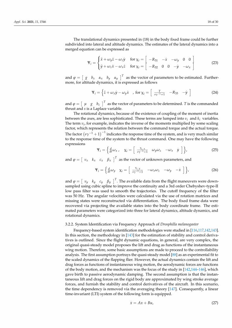
In the underlying strategy, the trim kinematics [99,142] were treated as periodic, rep-resented by φ(t), in a stroke plane, which makes an angle β with the horizontal. Boththe left and right wing were actuated simultaneously with the same control input for thesaid longitudinal motions. The control inputs were defined as stroke plane inclinationβc = 1

2 (βR + βL) [117,148], stroke plane offset φ0 f f = 12

(φ0 f fR + φ0 f fL

)[143,148], and

asymmetric wing angle αad = 12 (αu − αd) [117,143,148]. These inputs are shown in Figure 5.

Appl. Sci. 2021, 11, x FOR PEER REVIEW 19 of 30

approximated by wing stroke average forces, and furnish the stability and control deriv-

atives of the aircraft. In this scenario, the time dependency is removed via the averaging

theory [147]. Consequently, a linear time-invariant (LTI) system of the following form is

equipped.

� = �� + ��, (27)

where ����� represents the state matrix; ����� is the control derivative matrix; and

�����[ 0, ∞) indicates the controlled input history and ����

�[ 0, ∞) points to the state

history of the system. The aforementioned components smoothen the way to system

identification. To obtain stability and control derivatives and to perform nonlinear sim-

ulations, the system was considered as a rigid body in combination with quasi-steady

aerodynamics and the state perturbations caused by the state deviation from the equilib-

rium. Similar work can be found in [142] where the quasi-steady aerodynamics formula-

tion was treated as state perturbation from a reference equilibrium condition via proper

definition of the wing tip speed and the wing angle attack. The current subsection fo-

cused on the study in [143], with the aerodynamic model outlined in [142], which in-

cluded the effects of the rotational and translational rigid body motions.

In the underlying strategy, the trim kinematics [99,142] were treated as periodic,

represented by ϕ(t), in a stroke plane, which makes an angle � with the horizontal. Both

the left and right wing were actuated simultaneously with the same control input for the

said longitudinal motions. The control inputs were defined as stroke plane inclination

�� =�

�(�� + ��) [117,148], stroke plane offset ���� =

�

�(�����

+ �����) [129,174], and

asymmetric wing angle ��� =�

�(�� − ��) [117,143,148]. These inputs are shown in Fig-

ure 5.

Figure 5. Definition of the different control inputs in longitudinal motions [143].

Note that the input ��, which physically represents the tilting of the stroke plane, is

used to generate the pitch moment and forward force [142], ���� physically represents

the force shift of the wing sweep for pitch moment generation and ��� in a similar way

represents the upstroke or downstroke asymmetry in wing angle relative to the stroke

plane. This input is used to generate the forward force.

The longitudinal dynamics of the insect were excited by applying the chirp signal at

each input. The overall transfer function was found via the spectral analysis of the input

transfer function ��(�) and the output transfer function ��(�).

��(�) =��(�)

��(�), (28)

For the sake of completion, the input/output response in terms of magnitude, phase,

and coherence for ���� to θ is shown in Figure 6. The haltere-based feedback on the pitch

axis was used to make the system matrix Hurwitz. The system identification strategy via

the frequency-based analysis is considered to be more powerful [142] than the analytical

linearization and computational based techniques because by coherence (), one may

Figure 5. Definition of the different control inputs in longitudinal motions [143].

Note that the input βc, which physically represents the tilting of the stroke plane, isused to generate the pitch moment and forward force [142], φo f f physically representsthe force shift of the wing sweep for pitch moment generation and αau in a similar wayrepresents the upstroke or downstroke asymmetry in wing angle relative to the strokeplane. This input is used to generate the forward force.

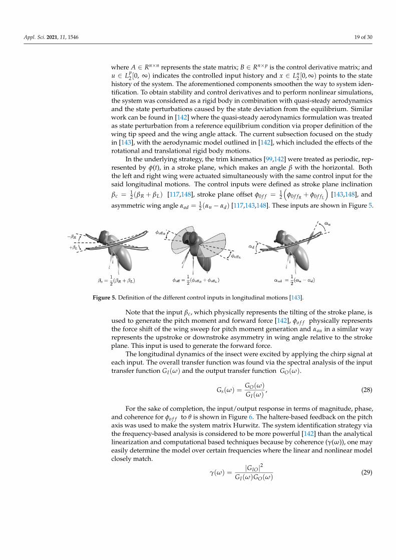
The longitudinal dynamics of the insect were excited by applying the chirp signal ateach input. The overall transfer function was found via the spectral analysis of the inputtransfer function GI(ω) and the output transfer function GO(ω).

Gs(ω) =GO(ω)

GI(ω), (28)

For the sake of completion, the input/output response in terms of magnitude, phase,and coherence for φo f f to θ is shown in Figure 6. The haltere-based feedback on the pitchaxis was used to make the system matrix Hurwitz. The system identification strategy viathe frequency-based analysis is considered to be more powerful [142] than the analyticallinearization and computational based techniques because by coherence (γ(ω)), one mayeasily determine the model over certain frequencies where the linear and nonlinear modelclosely match.

γ(ω) =|GIO|2

GI(ω)GO(ω)(29)

Appl. Sci. 2021, 11, 1546 20 of 30

Appl. Sci. 2021, 11, x FOR PEER REVIEW 20 of 30

easily determine the model over certain frequencies where the linear and nonlinear

model closely match.

�(�) =|���|�

��(�)��(�) (29)

Figure 6. The system identification block diagram for the full nonlinear model of Drosophila Mela-

nogaster flight dynamics [117].

The stability and control derivatives, in the forthcoming general state space model,

were determined at low frequency regions (0–20 Hz) by maximizing the coherence. In

addition, the small periodic high frequency motions were neglected in this range of fre-

quencies. The resulting mathematical model for longitudinal dynamics is shown by

Equation (30).

�

Δ�Δ�Δ�

Δ�

� = �

�� 0 0 −�0 �� 0 0

�� 0 �� 0

0 0 1 0

� �

ΔuΔ�ΔqΔθ

� + �

0 �� ���������

�� 0 0 00 �� �� ��

0 0 0 0

� �

Φ�

��

����

���

� (30)

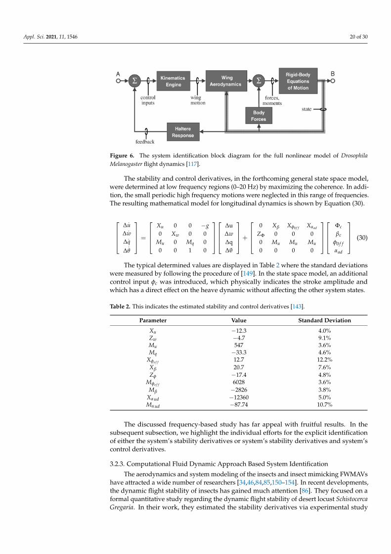
The typical determined values are displayed in Table 2 where the standard devia-

tions were measured by following the procedure of [149]. In the state space model, an

additional control input ϕ� was introduced, which physically indicates the stroke am-

plitude and which has a direct effect on the heave dynamic without affecting the other

system states.

Table 2. This indicates the estimated stability and control derivatives [143].

Parameter Value Standard Deviation

uX -12.3 4.0%

wZ -4.7 9.1%

uM 547 3.6%

qM -33.3 4.6%

offX 12.7 12.2%

X 20.7 7.6%

Z -17.4 4.8%

offM 6028 3.6%

M -2826 3.8%

udX -12360 5.0%

udM -87.74 10.7%

The discussed frequency-based study has far appeal with fruitful results. In the

subsequent subsection, we highlight the individual efforts for the explicit identification

Figure 6. The system identification block diagram for the full nonlinear model of DrosophilaMelanogaster flight dynamics [117].

The stability and control derivatives, in the forthcoming general state space model,were determined at low frequency regions (0–20 Hz) by maximizing the coherence. In addi-tion, the small periodic high frequency motions were neglected in this range of frequencies.The resulting mathematical model for longitudinal dynamics is shown by Equation (30).

∆

.u

∆.

w∆

.q

∆.θ

=

Xu 0 0 −g0 Xw 0 0

Mu 0 Mq 00 0 1 0

∆u∆w∆q∆θ

+

0 Xβ Xφ0 f f Xαad

ZΦ 0 0 00 Mu Mu Mu

0 0 0 0

Φc

βc

φ0 f fαad

(30)

The typical determined values are displayed in Table 2 where the standard deviationswere measured by following the procedure of [149]. In the state space model, an additionalcontrol input φc was introduced, which physically indicates the stroke amplitude andwhich has a direct effect on the heave dynamic without affecting the other system states.

Table 2. This indicates the estimated stability and control derivatives [143].

Parameter Value Standard Deviation

Xu −12.3 4.0%Zw −4.7 9.1%Mu 547 3.6%Mq −33.3 4.6%

Xφo f f 12.7 12.2%Xβ 20.7 7.6%Zφ −17.4 4.8%

Mφo f f 6028 3.6%Mβ −2826 3.8%

Xαud −12360 5.0%Mαud −87.74 10.7%

The discussed frequency-based study has far appeal with fruitful results. In thesubsequent subsection, we highlight the individual efforts for the explicit identificationof either the system’s stability derivatives or system’s stability derivatives and system’scontrol derivatives.

3.2.3. Computational Fluid Dynamic Approach Based System Identification

The aerodynamics and system modeling of the insects and insect mimicking FWMAVshave attracted a wide number of researchers [34,46,84,85,150–154]. In recent developments,the dynamic flight stability of insects has gained much attention [86]. They focused on aformal quantitative study regarding the dynamic flight stability of desert locust SchistocercaGregaria. In their work, they estimated the stability derivatives via experimental study

Appl. Sci. 2021, 11, 1546 21 of 30

that were further studied for eigenvalue analysis to recognize different stability modeslike the unstable oscillatory mode, stable fast subsidence, and slow subsidence mode.Note that the experiment carried out was subjected to some limitations such as that theinsect had to be tethered and the reference flight might not have been in equilibrium. Inpractice, the presence of such limitations may make the estimation of some morphologicalparameters impossible. In order to pave the way to estimate stability derivatives for allconditions and different flight maneuvers, [112] presented a CFD approach to measure thestability derivatives of a hovering bumblebee while capturing the flight data used in thestudy of [84,85], and the stability derivatives of beetle-mimicking FWMAV in [155]. In thisstudy, they first determined the equilibrium condition, while taking account of the rigidbody assumption, and utilized the flow equations and solution methodology presentedin [48] to compute the stability derivatives for the longitudinal flight dynamics. In thestability analysis, once again, they identified the same mode as were concluded in [86].In [156], the work of [112] was extended to carry out a formal analysis of the stability,controllability, and the stabilizing control of the hovering insect. The stability analysisresulted in the same modes as identified in [86]. Therefore, a control action in the feedbackloop was needed to stabilize the unstable oscillatory mode, and stability augmentationwas pursued for the slow subsidence mode. The stabilization was done by feeding back acontrolled input (i.e., the changes in the mean stroke angle as a function of pitch attitude,pitch rate, and horizontal velocity), whereas the second case was handled via a feedbackcontrol input (i.e., the changes in the stroke amplitude as a function of vertical velocity).This study was fascinating for further study in different flight envelopes. In the contextof longitudinal stability analysis, in [111], the dynamic stability of the beetle-mimickingFWMAVs [43] was investigated. The authors followed the trim condition determinationstrategy of [86], and CFD based stability derivatives were computed. The stability analysiswas concluded as very similar to [86,111]. In order to determine the flight stability, oneneeds to have the identified dynamics for both longitudinal and lateral motions. Currently,a quantitative analysis for the lateral dynamic stability of a hovering insect is addressedin [157] via the CFD strategy [111,156]. In this case, they focused on the drone fly insteadof the bumblebee. They have computed the stability derivatives and, once again, theeigenvalue-based analysis was conducted, and very similar results to the longitudinalscenario (i.e., one unstable slow divergence mode, one stable slow oscillatory mode, and astable fast subsidence mode) were identified. The aforementioned CFD strategies provide asuitable understanding about the stability analyses of FWMAVs. However, the CFD-basedapproach is computationally costly and time-consuming.

3.2.4. Parameter Estimation for Linear Damping Model of DelFly Nimble

The tailless version of DelFly, known as DelFly Nimble, was used in closed-loopmodeling of the longitudinal dynamics of a tailless flapping wing robot [158]. The ideaof the modeling is to investigate the effect of changing the robot physical parameters andthe controller gains to the robot’s flight dynamics. Due to the lack of tail that providespassive stabilization, the robot relies on the wing actuation system and active controlsystem to provide its stability and control. The linear damping model was selected as itcan approximate the aerodynamics of complex flapping wings with a minimal numberof parameters in hovering and forward cruise flight (with quasi-steady assumption) thatwere measured in a wind tunnel, as shown in [139,159]. It has also proven its ability inpredicting the horizontal drag forces of flapping wings. In [158], vertical dynamics andpitch control mechanisms were included. The overall model structure consists of controllerdynamics and open loop dynamics, which are comprised of the actuator dynamics and thelongitudinal flight dynamics.

Appl. Sci. 2021, 11, 1546 22 of 30

System identification was used to determine the dihedral actuator dynamics andforce coefficients, bx and bz, which define the longitudinal and vertical components of theaerodynamic drag forces as described by the following equations.

Dx = −bx f u,Dz = −bz f w,

where f is the flapping frequency; u and w are the longitudinal and vertical body velocities,respectively. Flight data were collected as the robot was flown in an open jet wind tunnelat various wind speeds ranging from 1 ms−1 to 2.4 ms−1. Both u and w were computedbased on the averaged wind speed and body pitch. Linear least squares method wasused to determine bx and bz. Validation was performed by comparing the estimated statederivatives from the model with those derived directly from the flight data. The overallresults show that the developed model can capture the robot’s dominant dynamic effectsand can be useful for initial tuning of the control parameters. The performance of thisapproach, however, will depend on the controller used.

4. Conclusions

A comprehensive review on system identification and mathematical modeling of flap-ping wing micro-aerial vehicles has been presented. The details were provided for taillessand tailed natural fliers and micro-aerial vehicles such as Drosophila, hawk ornithopter,RoboBee, KUBettle, and Delfly-II as well as the Delfly Nimble. The outcomes of the systemidentification approaches in all reviewed articles were satisfactory in general. The obtainedmodels were validated to predict and/or estimate the dynamics of the plants used, andthey could achieve reasonable accuracies. The identification strategies that have been usedwere top-down Grey box approaches. These include the extended Kalman Filter, linearregression and least square estimation, frequency-based identification, and computationalfluid dynamic based system identification. Most of the approaches were used to estimatemodel parameters that are related to aerodynamics and result in standard aircraft mathe-matical models or equations of motion, which are adopted with or without modifications.The modifications were based on a priori knowledge of the natural fliers’ aerodynamicsand engineering insights. The final models typically involve decoupling of the longitudinaland lateral dynamics. Additionally, wind tunnel or CFD-based system identification hasbeen mostly performed to determine the stability derivatives, which were then again usedtogether with the conventional aircraft equations of motion. CFD-based procedures wereperformed on the tested MAVs, while they were either mounted on a fixed platform or weretethered, thus, the natural flight motions of the vehicles were constrained, and this wouldchange the aerodynamics during the flight. The final mathematical model would be eithera full-model or a reduced model, in which insignificant stability derivatives were removed.Moreover, we found that a more complete system identification process aimed for designdecision and controller development was presented in [159], in which a simplified lineardamping model of the DelFly Nimble was obtained.

This review has shown that system identification approaches have a promising poten-tial to uncover many unanswered questions in generating valid mathematical models ofFWMAVs that can capture the overall FWMAVs’ complex flight dynamics. From the review,we conclude that system identification approaches have not been used to their maximumadvantage for modeling FWMAVs at the present stage. The approaches were mostly usedto obtain the aerodynamic parameters of certain FWMAVs for hovering and/or steadyflight, linear regression and least square estimation were mostly used, and the acquiredmodels were mostly linear. Thus, they are valid only for particular flight modes. Thereare still questions on the fidelity of the models obtained, particularly those for variousmaneuvers.

Better outcomes of system identification and modeling complex systems such as FW-MAVs can be achieved with detailed analyses done before the start of the identification thatlead to appropriate model selection. Such analysis will be critical to determine the opti-

Appl. Sci. 2021, 11, 1546 23 of 30

mized model structure and model order where a priori knowledge and engineering insightsare combined with formal properties of models. In addition, it is imperative to have clearobjectives of the system identification to be performed, for example, system identificationfor design decision, simulation or validation, and/or for flight control design. Therefore,specific experimental data, efficient model selection, and structure as well as identificationapproach can be determined accordingly. Many nonlinear system identification approachesthat are known for their powerful capabilities in dealing with nonlinear dynamical systemssuch as the unscented Kalman filter (UKF) and nonlinear autoregressive moving averagemodel with exogenous inputs (NARMAX) have not been considered to solve the modelingproblems of FWMAVs. Together with a priori knowledge and engineering insights, thoseapproaches are expected to provide more accurate outcomes than those of the linear ones.

Furthermore, there have hardly been any black-box approaches such as neural-network based system identification reported in use for the system identification of FW-MAVs. Such approaches have been used in the identification of other types of unmannedaerial vehicles such as in [160]. In conclusion, more sophisticated system identificationstrategies, combined with knowledge of aerodynamics and flight dynamics of naturalflapping wing fliers, should be utilized, so that we can gain more understanding of highlycomplex dynamics of FWMAVs, particularly to achieve the autonomous flight of FW-MAVs, and develop energy storage mechanisms to obtain energy efficient flight of insectfliers [161].

5. Future Works

Finally, this review article is furnished via our understudy theoretical strategy forsystem identification. This strategy followed the Grey box approach while utilizing the dif-ferentiator observer theory [162]. We proposed a sliding mode-based system identificationthat utilizes the robust and accurate nature of sliding mode observer and flatness property.The proposed technique is briefly discussed in this section. The motivation for the use ofthe aforementioned technique is its inherent robustness in the face of uncertain conditions.In this work, we also relax the identifiability condition [163]. At this point, the followingassumptions are furnished.

1. It is assumed that the control input derivatives are known and certain.2. The system’s stability derivatives are assumed to be unknown and separable.3. The states of the system are observable.4. The system under study must satisfy the flatness property [164].

Before proceeding to the stability derivative estimation, the observability and separa-bility conditions are checked offline. The flatness property plays a significant role in thisstrategy based on which parameters are extracted. The controller used in the closed-loopestimation is the one designed via sliding mode control strategy [165]. The identificationstrategy flowchart is shown in Figure 7. At the first step, the mathematical model ofthe system is developed and some parameters are marked as unknown in an uncertainenvironment. Then, by utilizing the flatness property, these parameters are extracted andare further estimated by invoking the known data. The mathematical model is finalized forcontrol design purpose by using these estimated parameters. Therefore, we can considerour strategy as the parameter identification of the flight dynamics of the FWMAVs.

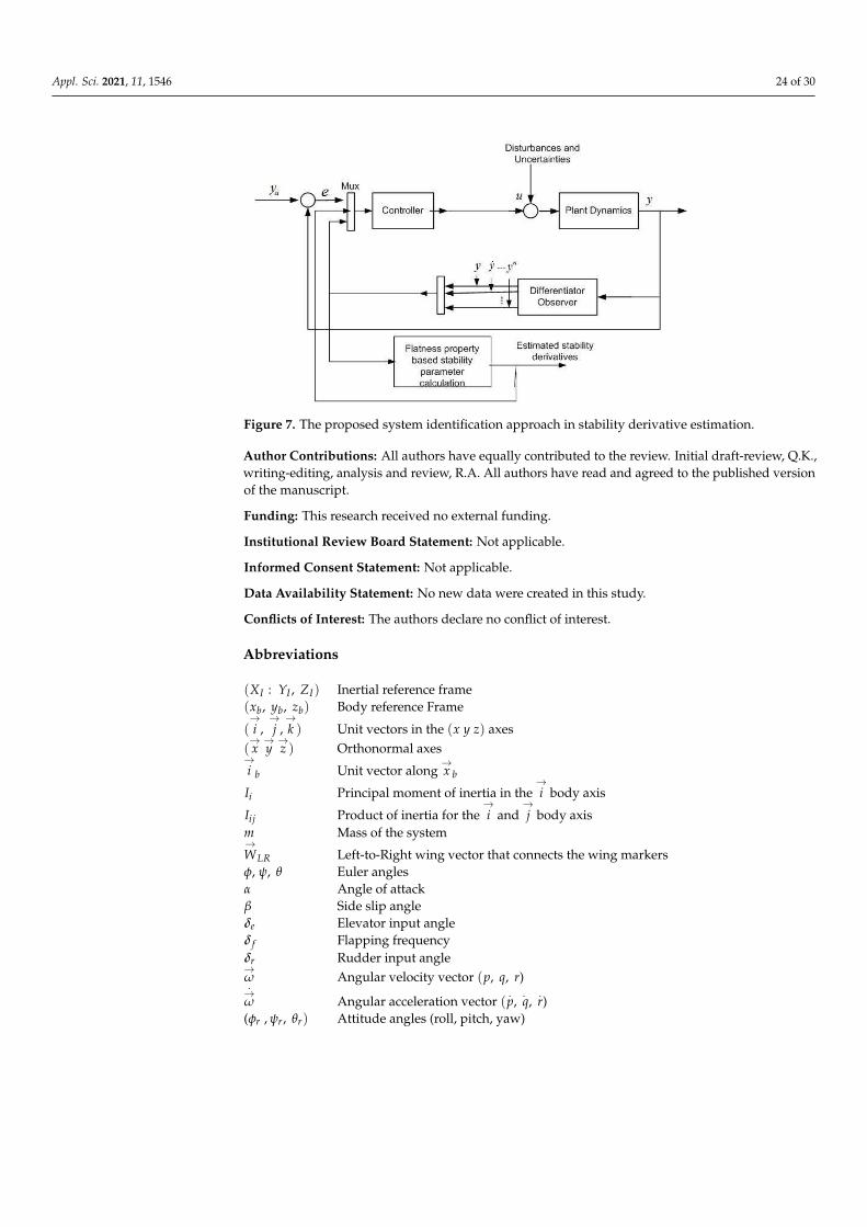
Appl. Sci. 2021, 11, 1546 24 of 30

Appl. Sci. 2021, 11, x FOR PEER REVIEW 24 of 30

model is finalized for control design purpose by using these estimated parameters.

Therefore, we can consider our strategy as the parameter identification of the flight dy-

namics of the FWMAVs.

Figure 7. The proposed system identification approach in stability derivative estimation.

Author Contributions: All authors have equally contributed to the review. Initial draft-review,

Q.K., writing-editing, analysis and review, R.A. All authors have read and agreed to the published

version of the manuscript.

Funding: This research received no external funding.

Institutional Review Board Statement: Not applicable.

Informed Consent Statement: Not applicable.

Data Availability Statement: No new data were created in this study.

Conflicts of Interest: The authors declare no conflict of interest.

Nomenclature

(��: ��, ��) Inertial reference frame

(��, ��, ��) Body reference Frame

(�, �, �� ) Unit vectors in the (� � �) axes

(� � �) Orthonormal axes

�� Unit vector along ��

�� Principal moment of inertia in the � body axis

��� Product of inertia for the � and � body axis

� Mass of the system

���� �� Left-to-Right wing vector that connects the wing markers

�, �, � Euler angles

� Angle of attack

� Side slip angle

�� Elevator input angle

�� Flapping frequency

�� Rudder input angle

��� Angular velocity vector(�, �, �)

��� Angular acceleration vector(�, �, �)

(�� , ��, ��) Attitude angles (roll, pitch, yaw)

∆ Difference between two consecutive time-steps

� External tracking system recording frequency

��� Standard rotation matrix from inertial to body frame

�, �, � Angular velocities in the (ı�, ȷ�, k� �) body axis

�, �, � Translational velocities in the (ı�, ȷ�, k� �) body axis

Figure 7. The proposed system identification approach in stability derivative estimation.

Author Contributions: All authors have equally contributed to the review. Initial draft-review, Q.K.,writing-editing, analysis and review, R.A. All authors have read and agreed to the published versionof the manuscript.

Funding: This research received no external funding.

Institutional Review Board Statement: Not applicable.

Informed Consent Statement: Not applicable.

Data Availability Statement: No new data were created in this study.

Conflicts of Interest: The authors declare no conflict of interest.

Abbreviations

(XI : YI , ZI) Inertial reference frame(xb, yb, zb) Body reference Frame

(→i ,→j ,→k ) Unit vectors in the (x y z) axes

(→x→y→z ) Orthonormal axes

→i b Unit vector along

→x b

Ii Principal moment of inertia in the→i body axis

Iij Product of inertia for the→i and

→j body axis

m Mass of the system→WLR Left-to-Right wing vector that connects the wing markersφ, ψ, θ Euler anglesα Angle of attackβ Side slip angleδe Elevator input angleδf Flapping frequencyδr Rudder input angle→ω Angular velocity vector (p, q, r).→ω Angular acceleration vector (

.p,

.q,

.r)

(φr , ψr, θr) Attitude angles (roll, pitch, yaw)

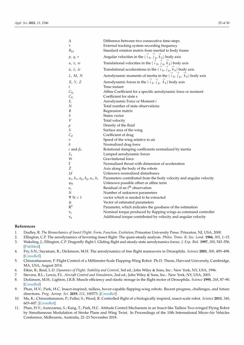
Appl. Sci. 2021, 11, 1546 25 of 30

∆ Difference between two consecutive time-stepsτ External tracking system recording frequencyRbI Standard rotation matrix from inertial to body frame

p, q, r Angular velocities in the (→i b,→j b,→k b) body axis

u, v, w Translational velocities in the (→i b,→j b,→k b) body axis

.u,

.v,

.w Translational accelerations in the (

→i b,→j b,→k b) body axis

L, M, N Aerodynamic moments of inertia in the (→i b,→j b,

→k b) body axis

X, Y, Z Aerodynamic forces in the (→i b,→j b,

→k b) body axis

t Time instantCF0 Affine Coefficient for a specific aerodynamic force or momentCFs Coefficient for state sFi Aerodynamic Force or Moment iN Total number of state observationsR Regression matrixS States vectorV Total velocityρ Density of the fluidS Surface area of the wingCd Coefficient of dragv Speed of the wing relative to airb Normalized drag forcec and βr Rotational damping coefficients normalized by inertiaFa Lumped aerodynamic forcesW Gravitational forceΓ Normalized thrust with dimension of accelerationZ Axis along the body of the robotsJd Unknown normalized disturbanceax, bx, ay, by, az, bz Parameters contributed from the body velocity and angular velocityϕ0 Unknown possible offset or affine termεi Residual of an ith observationN Number of unknown parametersΨ N× 1 vector which is needed to be extractedϕ Vector of estimated parametersR2 Parameter, which indicates the goodness of the estimationτc Nominal torque produced by flapping wings as command controllerτa Additional torque contributed by velocity and angular velocity

References1. Dudley, R. The Biomechanics of Insect Flight: Form, Function, Evolution; Princeton University Press: Princeton, NJ, USA, 2000.2. Ellington, C.P. The aerodynamics of hovering insect flight: The quasi-steady analysis. Philos. Trans. R. Soc. Lond. 1984, 305, 1–15.3. Wakeling, J.; Ellington, C.P. Dragonfly flight I. Gliding flight and steady-state aerodynamics forces. J. Exp. Biol. 1997, 200, 543–556.

[PubMed]4. Fry, S.N.; Sayaman, R.; Dickinson, M.H. The aerodynamics of free flight maneuvers in Drosophila. Science 2003, 300, 495–498.

[CrossRef]5. Chirarattananon, P. Flight Control of a Millimeter-Scale Flapping-Wing Robot. Ph.D. Thesis, Harvard University, Cambridge,

MA, USA, August 2014.6. Etkin, B.; Reid, L.D. Dynamics of Flight: Stability and Control, 3rd ed.; John Wiley & Sons, Inc.: New York, NY, USA, 1996.7. Stevens, B.L.; Lewis, F.L. Aircraft Control and Simulation, 2nd ed.; John Wiley & Sons, Inc.: New York, NY, USA, 2003.8. Dickinson, M.H.; Lighton, J.R.B. Muscle efficiency and elastic storage in the flight motor of Drosophila. Science 1995, 268, 87–90.

[CrossRef]9. Phan, H.V.; Park, H.C. Insect-inspired, tailless, hover-capable flapping-wing robots: Recent progress, challenges, and future

directions. Prog. Aerosp. Sci. 2019, 111, 100573. [CrossRef]10. Ma, K.; Chirarattananon, P.; Fuller, S.; Wood, R. Controlled flight of a biologically inspired, insect-scale robot. Science 2013, 340,

603–607. [CrossRef]11. Phan, H.V.; Aurecianus, S.; Kang, T.; Park, H.C. Attitude Control Mechanism in an Insect-like Tailless Two-winged Flying Robot

by Simultaneous Modulation of Stroke Plane and Wing Twist. In Proceedings of the 10th International Micro-Air VehiclesConference, Melbourne, Australia, 22–23 November 2018.

Appl. Sci. 2021, 11, 1546 26 of 30

12. Karasek, M. Robotic Hummingbird: Design of a Control Mechanism for a Hovering Apping Wing Micro Air Vehicle. Ph.D.Thesis, Universite Libre de Bruxelles, Brussels, Belgium, 2014.

13. Malolan, V.; Dineshkumar, M.; Baskar, V. Design and development of flapping wing micro air-vehicles. In Proceedings of the42nd AIAA Aerospace Science Meeting and Exhibits, Reno, Nevada, 5–8 January 2004.

14. Festo. Festo-Smart Bird Inspired by Nature. 2011. Available online: https://www.festo.com/group/en/cms/10238.htm (accessedon 30 October 2020).

15. Keennon, M.; Klingebiel, K.; Won, H.; Andriukov, A. Development of the nano-hummingbird: A tailless flapping wing microair vehicle. In Proceedings of the 50th AIAA Aerospace Sciences Meeting including the New Horizons Forum and AerospaceExposition, Nashville, TN, USA, 9–12 January 2012; pp. 1–24.

16. Ristroph, L.; Childress, S. Stable hovering of a jellyfish-like flying machine. J. R. Soc. Interface 2014, 11, 20130992. [CrossRef]17. De Croon, G.C.H.E.; De Clercq, K.M.E.; Ruijsink, R.; Remes, B.; De Wagter, C. Design, aerodynamics, and vision-based control of

the Delfly. Int. J. Micro Air Veh. 2009, 1, 71–97. [CrossRef]18. Wood, R.J. The first takeoff of a biologically inspired at-scale robotic insect. IEEE Trans. Robot. 2008, 24, 341–347.19. Finio, B.M.; Wood, R.J. Open-loop roll, pitch and yaw torques for a Robotic Bee. In Proceedings of the IEEE/RSJ International

Conference on Intelligent Robots and Systems, Algarve, Portugal, 7–12 October 2012; pp. 113–119.20. Ma, K.Y.; Felton, S.M.; Wood, R.J. Design, fabrication, and modeling of the split actuator micro-robotic bee. In Proceedings of the

IEEE/RSJ International Conference on Intelligent Robots and Systems, Algarve, Portugal, 7–12 October 2012; pp. 1133–1140.21. Ramasamy, M.; Leishman, J.G.; Lee, T.E. Flow field of a rotating wing micro air vehicle. J. Aircr. 2007, 44, 1236–1244. [CrossRef]22. Gaissert, N.; Mugrauer, R.; Mugrauer, G.; Jebens, A.; Jebens, K.; Knubben, E.M. Inventing a micro aerial vehicle inspired by the

mechanics of dragonfly flight. In Towards Autonomous Robotic Systems; TAROS 2013. Lecture Notes in Computer Science; Springer:Berlin/Heidelberg, Germany, 2014; Volume 8069, pp. 90–100.

23. Baek, S.S. Autonomous Ornithopter Flight with Sensor-Based Behavior; Univ. California, Berkeley, UC Berkeley: Berkeley, CA, USA,ProQuest ID: Baek_berkeley_0028E_11581. Merritt ID: Ark:/13030/m5sf314b; 2011; Available online: https://escholarship.org/uc/item/8f83m0xp.

24. Baek, S.; Fearing, R. Flight forces and altitude regulation of 12gram i-bird. In Proceedings of the IEEE RAS and EMBS InternationalConference on Biomedical Robotics and Biomechatronics (BioRob), Tokyo, Japan, 26–29 September 2010; pp. 454–460.

25. De Croon, G.C.H.E.; Groen, M.A.; De Wagter, C.; Remes, B.; Ruijsink, R.; Van Oudheusden, B. Design, aerodynamics, andautonomy of the Delfly. Bioinspir. Biomimet. 2012, 7, 025003. [CrossRef] [PubMed]

26. De Croon, G.; De Weerdt, E.; De Wagter, C.; Remes, B.; Ruijsink, R. The appearance variation cue for obstacle avoidance. IEEETrans. Robot. 2012, 28, 529–534. [CrossRef]

27. Tijmons, S.; De Croon, G.; Remes, B.; De Wagter, C.; Ruijsink, R.; van Kampen, E.J.; Chu, Q.P. Stereo-vision based obstacleavoidance on flapping wing MAV. In Advances in Aerospace Guidance, Navigation and Control; Chu, Q., Mulder, B., Choukroun, D.,van Kampen, E.J., de Visser, C., Looye, G., Eds.; Springer: Berlin/Heidelberg, Germany, 2013.

28. Mueller, D.; Gerdes, J.; Gupta, S.K. Incorporation of passive wing folding in flapping wing miniature air vehicles. In Proceedingsof the ASME Robotics and Mechatronics Conference, San Diego, CA, USA, 30 August–2 September 2009.

29. Yang, L.J. The Micro-Air-Vehicle Golden Snitch and Its Figure-of-8 Flapping. J. Appl. Sci. Eng. 2012, 15, 197–212.30. Ellington, C.P. The aerodynamics of hovering insect flight. III. Kinematics. Philos. Trans. R. Soc. Lond. 1984, B305, 41–78.31. Willmott, A.P.; Ellington, C.P. Measuring the angle of attack of beating insect wings: Robust three-dimensional reconstruction

from two dimensional images. J. Exp. Biol. 1997, 200, 2693–2704.32. Cloupeau, M.; Devillers, J.F.; Devezeaux, D. Direct measurements of instantaneous lift in desert locust; comparison with Jensen’s

experiments on detached wings. J. Exp. Biol. 1979, 80, 1–15.33. Buckholz, R.H. Measurements of unsteady periodic forces generated by the blowfly flying in a wind tunnel. J. Exp. Biol. 1981, 90,

163–173.34. Somps, C.; Luttges, M. Dragonfly flight—novel uses of unsteady separated flows. Science 1985, 228, 1326–1329. [CrossRef]35. Zanker, J.M.; Gotz, K.G. The wing beat of Drosophila melanogaster II. Dynamics. Philos. Trans. R. Soc. Lond. 1990, B327, 19–44.36. Wilkin, P.J.; Williams, M.H. Comparison of the instantaneous aerodynamic forces on a sphingid moth with those predicted by

quasi-steady aerodynamic theory. Physiol. Zool. 1993, 66, 1015–1044. [CrossRef]37. Bennett, L. Insect flight: Lift and the rate of change of incidence. Science 1970, 167, 177–179. [CrossRef] [PubMed]38. Maxworthy, T. Experiments on the Weis-Fogh mechanism of lift generation by insects in hovering flight. Part 1. Dynamics of the

‘fling’. J. Fluid Mech. 1979, 93, 47–63. [CrossRef]39. Spedding, G.R.; Maxworthy, T. The generation of circulation and lift in a rigid two-dimensional fling. J. Fluid Mech. 1986, 165,

247–272. [CrossRef]40. Dickinson, M.H.; Götz, K.G. Unsteady aerodynamic performance of model wings at low Reynolds numbers. J. Exp. Biol. 1993,

174, 45–64.41. Sunada, S.; Kawachi, K.; Watanabe, I.; Azuma, A. Fundamental analysis of 3-dimensional near fling. J. Exp. Biol. 1993, 183,

217–248.42. Ellington, C.P. The novel aerodynamics of insect flight: Applications to micro-air vehicles. J. Exp. Biol. 1999, 202, 3439–3448.43. Dickinson, M.H.; Lehmann, F.-O.; Sane, S.P. Wing rotation and the aerodynamic basis of insect flight. Science 1999, 284, 1954–1960.

[CrossRef]

Appl. Sci. 2021, 11, 1546 27 of 30

44. Liu, H.; Ellington, C.P.; Kawachi, K.; Van den Berg, C.; Willmott, A.P. A computational fluid dynamic study of hawkmothhovering. J. Exp. Biol. 1998, 201, 461–477.

45. Liu, H.; Kawachi, K. A numerical study of insect flight. J. Comput. Phy. 1998, 146, 124–156. [CrossRef]46. Wang, Z.J. Two-dimensional mechanism for insect hovering. Phys. Rev. Lett. 2000, 85, 2216–2219. [CrossRef]47. Ramamurti, R.; Sandberg, W.C. A three-dimensional computational study of the aerodynamic mechanisms of insect flight. J. Exp.

Biol. 2002, 205, 1507–1518. [PubMed]48. Sun, M.; Tang, J. Unsteady aerodynamic force generation by a model fruit fly wing in flapping motion. J. Exp. Biol. 2002, 205,

55–70. [PubMed]49. Taha, H.E.; Hajj, M.R.; Nayfeh, A.H. Flight dynamics and control of flapping-wing MAVs: A review. Nonlinear Dyn. 2012, 70,

907–939. [CrossRef]50. Sun, M. Insect flight dynamics: Stability and control. Rev. Mod. Phys. 2014, 86, 615–646. [CrossRef]51. Taylor, G.K. Mechanics and aerodynamics of insect flight control. Biol. Rev. 2001, 76, 449–471. [CrossRef] [PubMed]52. Orlowski, C.T.; Girard, A.R. Dynamics, Stability and Control an analyses of flapping wing micro air vehicles. Progr. Aerosp. Sci.

2012, 51, 18–30. [CrossRef]53. Zadeh, L.A. On the identification problem. IRE Trans. Circuit Theory 1956, 3, 277–281. [CrossRef]54. Xiao, X.; Mullen, T.; Mukkamala, R. System Identification: A multi-signal approach for probing neural cardiovascular regulation,

Phys. Meas. 2005, 26, R41–R71. [CrossRef]55. Morelli, E.A.; Klein, V. Aircraft System Identification: Theory and Practice; AIAA Education Series; AIAA: Reston, VA, USA, 2006.56. Lai, Y.-C.; Ting, W.O. Design and Implementation of an Optimal Energy Control System for Fixed-Wing Unmanned Aerial

Vehicles. Appl. Sci. 2016, 6, 369. [CrossRef]57. Naeem, W.; Sutton, R.; Chudley, J. System Identification, Modelling and Control of an Autonomous Underwater Vehicle. IFAC

Proc. 2003, 36, 19–24. [CrossRef]58. Ljung, L. System Identification Theory for the User, 2nd ed.; Prentice Hall: Englewood Cliffs, NJ, USA, 1999.59. Ghiaus, C.; Ghazal, R.; Joubert, P.; Hayyani, M.Y. Gray-box state-space model and parameter identification of desiccant wheels. J.

Appl. Therm. Eng. 2013, 51, 742–752. [CrossRef]60. Shyy, W.; Lian, Y.; Tang, J.; Viieru, D.; Liu, H. Aerodynamics of Low Reynolds Number Fliers; Cambridge University Press: New York,

NY, USA, 2008.61. Norberg, U.M.L. Structure, form, and function of flight in engineering and the living world. J. Morphol. 2002, 252, 52–81.

[CrossRef] [PubMed]62. Shyy, W.; Aono, H.; Kang, C.K.; Liu, H. An Introduction to Flapping Wing Aerodynamics; Cambridge University Press: New York,

NY, USA, 2013.63. Sun, M.; Wu, J.H. Aerodynamic force generation and power requirements in forward flight in a fruit fly with modeled wing

motion. J. Exp. Biol. 2003, 206, 3065–3083. [CrossRef] [PubMed]64. Azuma, A. The Biokinetics of Flying and Swimming, 2nd ed.; AIAA Education Series; AIAA: Reston, VA, USA, 2006.65. Muijres, F.T.; Johansson, L.; Bareld, R.; Wolf, M.; Spedding, G.; Hedenstrm, A. Leading-edge vortex improves lift in slow-flying

bats. Science 2008, 319, 1250–1253. [CrossRef] [PubMed]66. Warrick, D.; Hedrick, T.; Fernndez, M.J.; Tobalske, B.; Biewener, A. Hummingbird flight. Curr. Biol. 2012, 22, 472–477. [CrossRef]67. Dickinson, M.H.; Dudley, R. Flight. In Encyclopedia of Insects, 2nd ed.; Academic Press: San Diego, CA, USA, 2009.68. Tennekes, H. The Simple Science of Flight: From Insects to Jumbo Jets; The MIT Press: Cambridge, MA, USA, 2009.69. Chin, D.D.; Lentink, D. Flapping wing aerodynamics: From insects to vertebrates. J. Exp. Biol. 2016, 219, 920–932.70. Shyy, W.; Kang, C.-k.; Chirarattananon, P.; Ravi, S.; Liu, H. Aerodynamics, sensing and control of insect-scale flapping-wing

flight. Proc. R. Soc. A 2015, 472, 20150712. [CrossRef]71. Ravi, S.; Noda, R.; Gagliardi, S.; Kolomenskiy, D.; Combes, S.; Liu, H.; Biewener, A.A.; Konow, N. Modulation of Flight Muscle

Recruitment and Wing Rotation Enables Hummingbirds to Mitigate Aerial Roll Perturbations. Curr. Biol. 2020, 30, 187–195.[CrossRef]

72. Knowles, K.; Phillips, N. Reynolds number and stroke amplitude effects on the leading-edge vortex on an insect-like flappingwing. In Proceedings of the International Powered Lift Conference, Philadelphia, PA, USA, 5–7 October 2010.

73. Weis-Fogh, T. Energetics of hovering flight in humming birds and drosophila. J. Exp. Biol. 1972, 56, 79–104.74. Weis-Fogh, T. Quick estimates of flight fitness in hovering animals, including novel mechanisms for lift production. J. Exp. Biol.

1973, 59, 169–230.75. Ellington, C.P. The aerodynamics of hovering insect flight II: Morphological parameters. Philos. Trans. R. Soc. Lond. 1984, 305,

17–40.76. Ellington, C.P. Aerodynamics and the Origin of Insect Flight. Adv. Insect Physiol. 1991, 23, 171–210.77. Ellington, C.P. The aerodynamics of hovering insect flight IV: Aerodynamic mechanisms. Philos. Trans. R. Soc. Lond. 1984, 305,

79–113.78. Ellington, C.P. The aerodynamics of hovering insect flight V: A vortex theory. Philos. Trans. R. Soc. Lond. 1984, 305, 115–144.79. Ellington, C.P. The aerodynamics of hovering insect flight VI: Lift and power requirements. Philos. Trans. R. Soc. Lond. 1984, 305,

145–181.

Appl. Sci. 2021, 11, 1546 28 of 30

80. Willmott, A.; Ellington, C.P. The mechanics of flight in the hawkmoth Manduca sexta i. Kinematics of hovering and forwardflight. J. Exp. Biol. 1997, 200, 2705–2722.

81. Cheng, B.; Deng, X.; Hedrick, T.L. The mechanics and control of pitching manoeuvres in a freely flying hawkmoth (manducasexta). J. Exp. Biol. 2011, 214, 4092–4106. [CrossRef]

82. Wakeling, J.; Ellington, C.P. Dragonfly flight II. Velocities, accelerations, and kinematics of flapping flight. J. Exp. Biol. 1997, 200,557–582.

83. Wakeling, J.; Ellington, C.P. Dragonfly flight III. Lift and power requirements. J. Exp. Biol. 1997, 200, 583–600.84. Dudley, R.; Ellington, C.P. Mechanics of forward flight in bumblebees I. Kinematics and morphology. J. Exp. Biol. 1990, 148, 19–52.85. Dudley, R.; Ellington, C.P. Mechanics of forward flight in bumblebees ii. Quasi-steady lift and power requirements. J. Exp. Biol.

1990, 148, 53–88.86. Taylor, G.K.; Thomas, A. Dynamic flight stability in the desert locus Schistocerca gregaria. J. Exp. Biol. 2003, 206, 2803–2829.

[CrossRef] [PubMed]87. Sane, S.; Dickinson, M. The control of flight force by a flapping wing: Lift and drag production. J. Exp. Biol. 2001, 204, 2607–2626.88. Sane, S.; Dickinson, M.H. The aerodynamic effects of wing rotation and a revised quasi-steady model of flapping flight. J. Exp.

Biol. 2002, 205, 1087–1096. [PubMed]89. Sane, S. Review: The aerodynamics of insect flight. J. Exp. Biol. 2003, 206, 4191–4208. [CrossRef] [PubMed]90. Wang, Z.J. Dissecting insect flight. Ann. Rev. Fluid. Mech. 2005, 37, 183–210. [CrossRef]91. Shyy, W.; Lian, Y.; Tang, J.; Liu, H.; Trizila, P.; Stanford, B. Computational aerodynamics of low Reynolds number plunging,

pitching and flexible wings for MAV applications. Act. Mech. Sin. 2008, 24, 351–373. [CrossRef]92. Karásek, M.; Preumont, A. Flapping Flight Stability in Hover: A Comparison of Various Aerodynamic Models. Int. J. Micro Air

Veh. 2012, 4, 203–226. [CrossRef]93. Caetano, J.V.; De Visser, C.C.; De Croon, G.C.H.E.; Remes, B.; De Wagter, C.; Verboom, J.; Mulder, M. Linear Aerodynamic Model

Identification of a Flapping Wing MAV based on Flight Test Data. Int. J. Micro Air Veh. 2013, 5, 273–286. [CrossRef]94. Caetano, J.V.; De Visser, C.C.; Remes, B.; De Wagter, C.; Mulder, M. Controlled flight maneuvers of a flapping wing micro air

vehicle: A step towards the DelFly II identication. In Proceedings of the AIAA Atmospheric Flight Mechanics Conference, Boston,MA, USA, 19–22 August 2013.

95. Zhu, J.Y.; Zhou, C.Y. Aerodynamic performance of a two-dimensional flapping wing in asymmetric stroke. J. Aerosp. Eng. 2014,228, 641–651. [CrossRef]

96. Wang, C.; Zhou, C.; Xie, P. Numerical investigation on aerodynamic performance of a 2-D inclined hovering wing in asymmetricstrokes. J. Mech. Sci. Technol. 2016, 30, 199–210. [CrossRef]

97. Kang, C.K.; Shyy, W. Analytical model for instantaneous lift and shape deformation of an insect-scale flapping wing in hover. J. R.Soc. Interface 2014, 11, 1–10. [CrossRef] [PubMed]

98. Bergou, A.J.; Xu, S.; Wang, Z.J. Passive wing pitch reversal in insect flight. J. Fluid Mech. 2007, 591, 321–337. [CrossRef]99. Berman, G.J.; Wang, Z.J. Energy-minimizing kinematics in hovering insect flight. J. Fluid Mech. 2007, 582, 153–168. [CrossRef]100. Cheng, B.; Deng, X. Translational and rotational damping of flapping flight and its dynamics and stability at hovering. IEEE

Trans. Robot. 2011, 27, 849–864. [CrossRef]101. Kim, J.K.; Han, J.H. A multibody approach for 6-dof flight dynamics and stability analysis of the hawkmoth Manduca Sexta.

Bioinspir. Biomimet. 2014, 9. [CrossRef]102. Zheng, L.; Hedrick, T.L.; Mittal, R. A multi-fidelity modeling approach for evaluation and optimization of wing stroke aerody-

namics in flapping flight. J. Fluid Mech. 2013, 721, 118–154. [CrossRef]103. Liu, H. Integrated modeling of insect flight: From morphology, kinematics to aerodynamics. J. Comput. Phys. 2009, 228, 439–459.

[CrossRef]104. Liu, H.; Aono, H. Size effects on insect hovering aerodynamics: An integrated computational study. Bioinspir. Biomimet. 2009, 4.

[CrossRef]105. Young, J.; Walker, S.M.; Bomphrey, R.J.; Taylor, G.K.; Thomas, A.L.R. Details of insect wing design and deformation enhance

aerodynamic function and flight efficiency. Science 2009, 325, 1549–1552. [CrossRef]106. Nakata, T.; Liu, H.; Bomphrey, R.J. A CFD-informed quasi-steady model of flapping-wing aerodynamics. J. Fluid Mech. 2015, 783,

323–343. [CrossRef]107. Le, T.Q.; Truong, T.V.; Tran, H.T.; Park, S.H.; Ko, J.H.; Park, H.C.; Yoon, K.J.; Byun, D. Two and Three-Dimensional Simulations of

Beetle Hind Wing Flapping during Free Forward Flight. J. Bionic Eng. 2013, 10, 316–328. [CrossRef]108. Le, T.Q.; Truong, T.V.; Tran, H.T.; Park, S.H.; Ko, J.H.; Park, H.C.; Byun, D. How Could Beetle’s Elytra Support Their Own Weight

during Forward Flight? J. Bionic Eng. 2014, 11, 529–540. [CrossRef]109. Koopmans, J.A.; Tijmons, S.; De Wagter, C.; De Croon, G. Passively Stable Flapping Flight from Hover to Fast Forward through

Shift in Wing Position. Int. J. Micro Air Veh. 2015, 7, 407–418. [CrossRef]110. Ward, T.A.; Rezadad, M.; Fearday, C.J.; Viyapuri, R. A Review of Biomimetic Air Vehicle Research: 1984–2014. Int. J. of Micro Air

Veh. 2015, 7, 375–394. [CrossRef]111. Au, L.T.K. Dynamic Flight Stability of the Vertically Flying Insect Mimicking Flapping Wing System. Master’s Thesis, Konkuk

University, Seoul, South Korea, 2013.112. Sun, M.; Xiong, Y. Dynamic flight stability of a hovering bumblebee. J. Exp. Biol. 2005, 208, 447–459. [CrossRef] [PubMed]

Appl. Sci. 2021, 11, 1546 29 of 30

113. Wood, R.J. Design, fabrication, and analysis, of a 3DOF flapping-wing MAV. In Proceedings of the IEEE/RSJ InternationalConference on Intelligent Robotics and Systems 2007, San Diego, CA, USA, 29 October–2 November 2007; pp. 1576–1581.

114. Whitney, J.P.; Wood, R.J. Aeromechanics of passive rotation in flapping flight. J. Fluid. Mech. 2010, 1, 1–24. [CrossRef]115. Wood, R.J.; Steltz, E.; Fearing, R.S. Nonlinear performance limits for high energy density piezoelectric bending actuators. In

Proceedings of the International Conference on Robotics and Automation, Barcelona, Spain, 18–22 April 2005; pp. 3633–3640.116. Fino, B.M.; Perez-Arancibia, N.O.; Wood, R.J. System Identification and Linear Time Invariant Modeling of an Insect Sized

Flapping Wing Micro Air Vehicle. In Proceedings of the 2011 IEEE/RSJ International Conference on Intelligent Robots andSystems, San Francisco, CA, USA, 25–30 September 2011; pp. 1107–1114.

117. Faruque, I. Control-Oriented Reduced Order Modeling of Dipteran Flapping Flight. Ph.D. Thesis, Faculty of the Graduate Schoolof the University of Maryland, College Park, MD, USA, 2011.

118. Khan, Z.; Agrawal, S. Modeling and simulation of flapping wing micro air vehicles. In Proceedings of the IDETC/CIE’2005 2005ASME International Design Engineering Technical Conferences, Long Beach, CA, USA, 24–28 September 2005.

119. Percin, M.; Hu, Y.; Van Oudheusden, B.; Remes, B.; Scarano, F. Wing flexibility effects in clap-and fling. Int. J. Micro Air Veh. 2011,3, 217–227. [CrossRef]

120. Percin, M.; Eisma, H.; Van Oudheusden, B.; Remes, B.; Ruijsink, R.; De Wagter, C. Flow visualization in the wake of the flapping-wing MAV ‘DelFly II’ in forward flight. In Proceedings of the 30th AIAA Applied Aerodynamics Conference, New Orleans, LA,USA, 25–28 June 2012.

121. Orlowski, C.T.; Girard, A.R. Modeling and simulation of nonlinear dynamics of flapping wing micro air vehicles. AIAA J. 2011,49, 969–981. [CrossRef]

122. Dietl, J.M.; Garcia, E. Stability in ornithopter longitudinal flight dynamics. J. Guid. Control Dyn. 2008, 31, 1157–1162. [CrossRef]123. Dietl, J.M.; Herrmann, T.; Reich, G.; Garcia, E. Dynamic modeling, testing, and stability analysis of an ornithoptic blimp. J. Bionic

Eng. 2011, 8, 375–386. [CrossRef]124. Dietl, J.M.; Garcia, E. Ornithopter optimal trajectory control. Aerosp. Sci. Technol. 2013, 26, 192–199. [CrossRef]125. Bolender, M.A. Rigid multi-body equations-of-motion for flapping wing MAVs using Kane equations. In Proceedings of the

AIAA Guidance, Navigation, and Control Conference, Chicago, IL, USA, 10–13 August 2009.126. Grauer, J.H. Modeling of ornithopter flight dynamics for state estimation and control. In Proceedings of the 2010 American

Control Conference, Baltimore, MD, USA, 30 June–2 July 2010; pp. 524–529.127. Grauer, J.; Ulrich, E.; Hubbard, J.E.; Pines, D.; Humbert, J.S. Testing and system identification of an ornithopter in longitudinal

flight. J. Aircr. 2011, 48, 660–667. [CrossRef]128. Caetano, J.V.; Verboom, J.; de Visser, C.C.; de Croon, G.C.H.E.; Remes, B.D.W.; de Wagter, C.; Mulder, M. Near Hover Flapping

Wing MAV Aerodynamic Modelling-a linear model approach. In Proceedings of the International Micro Air Vechicle Conferenceand Flight Competition, Toulouse, France, 17–20 September 2017.

129. Mulder, J.A.; Chu, Q.P.; Sridhar, J.K.; Breeman, J.H.; Laban, M. Non-linear aircraft flight path reconstruction review and newadvances. Prog. Aerosp. Sci. 1999, 35, 673–726. [CrossRef]

130. Au, L.T.K.; Park, H.C. Influence of Center of Gravity Location on Flight Dynamic Stability in a Hovering Tailless FW-MAV:Longitudinal Motion. J. Bionic Eng. 2019, 16, 130–144. [CrossRef]

131. Au, L.T.K.; Park, H.C. Influence of Center of Gravity Location on Flight Dynamic Stability in a Hovering Tailless FW-MAV: LateralMotion. J. Bionic Eng. 2020, 17, 148–160. [CrossRef]

132. Caetano, J.V.; Weehuizen, M.B.; De Visser, C.C.; De Croon, G.C.H.E.; De Wagter, C.; Remes, B.; Mulder, M. Rigid vs. Flapping:The Effects of Kinematic Formulations in Force Determination of a Free Flying Flapping Wing Micro Air Vehicle. In Proceedingsof the International Conference on Unmanned Aircraft Systems (ICUAS), Orlando, FL, USA, 27–30 May 2014.

133. Caetano, J.V.; Percinz, M.; de Visser, C.C.; van Oudheusdenz, B.; de Croon, G.C.H.E.; de Wagter, C.; Remes, B.; Mulder, M.Tethered vs. Free Flight Force Determination of the DelFly II Flapping Wing Micro Air Vehicle. In Proceedings of the InternationalConference on Unmanned Aircraft Systems (ICUAS), Orlando, FL, USA, 27–30 May 2014.

134. Armanini, S.F.; Karasek, M.; de Croon, G.C.H.E.; de Visser, C.C. Onboard/Offboard Sensor Fusion for High-Fidelity Flapping-Wing MAV Flight Data. AIAA J. Guid. Control Dyn. 2017, 40, 2121–2132. [CrossRef]

135. Grauer, J. Modeling and System Identification of an Ornithopter Flight Dynamics Model. Ph.D. Thesis, University of Maryland,College Park, MD, USA, 2012.

136. Hoburg, W.; Tedrake, R. System identification of post stall aerodynamics for UAV perching. In Proceedings of the AIAAInfotech@Aerospace Conference, Seattle, WA, USA, 6–9 April 2009.

137. Forssell, U.; Ljung, L. Closed-loop identification revisited. Automatica 1999, 35, 1215–1241. [CrossRef]138. Gustavsson, I.; Ljung, L.; Söderström, T. Identification of processes in closed loop-identifiability and accuracy aspects. Automatica

1977, 13, 59–75. [CrossRef]139. Chirarattananon, P.; Wood, R.J. Identification of flight aerodynamics for flapping-wing microrobots. In Proceedings of the

International Conference on Robotics and Automation (ICRA), Karlsruhe, Germany, 6–10 May 2013; pp. 1389–1396.140. Ristroph, L.; Bergou, A.J.; Guckenheimer, J.; Wang, Z.J.; Cohen, I. Paddling mode of forward flight in insects. Phy. Rev. Lett. 2011,

106, 178103. [CrossRef]141. Ristroph, L.; Ristroph, G.; Morozova, S.; Bergou, A.J.; Chang, S.; Guckenheimer, J.; Wang, Z.J.; Cohen, I. Active and passive

stabilization of body pitch in insect flight. J. R. Soc. Interface 2013, 10, 20130237. [CrossRef]

Appl. Sci. 2021, 11, 1546 30 of 30

142. Faruque, A.I.; Humbert, J.S. Dipteran Insect Flight Dynamics Part 1: Longitudinal Motion about Hover. J. Theor. Biol. 2010, 264,538–552. [CrossRef]

143. Humbert, J.S.; Faruque, I. Analysis of Insect-Inspired Wingstroke Kinematic Perturbations for Longitudinal Control. AIAA J.Guid. Control Dyn. 2011, 34, 618–623. [CrossRef]

144. Cheng, B.; Fry, S.N.; Huang, Q.; Dickson, W.B. Turning Dynamics and Passive Damping in Flapping Flight. In Proceedings of the2009 IEEE International Conference on Robotics and Automation, Kobe, Japan, 12–17 May 2009.

145. Hesselberg, T.; Lehmann, F.O. Turning Behaviour Depends on Frictional Damping in the Fruit Fly Drosophila. J. Exp. Biol. 2007,210, 4319–4334. [CrossRef] [PubMed]

146. Taylor, G.K.; Thomas, A.L.R. Animal Flight Dynamics II. Longitudinal Stability in Flapping Flight. J. Theor. Biol. 2002, 214,351–370. [CrossRef] [PubMed]

147. Deng, X.; Schenato, L.; Sastry, S.S. Flapping Flight for Biomimetic Robotic Insects: Part II, Flight Control Design. IEEE Trans.Robot. Autom. 2006, 22, 789–803. [CrossRef]

148. Faruque, I.A.; Muijres, F.T.; Macfarlane, K.M.; Kehlenbeck, A.; Humbert, J.S. Identification of optimal feedback control rules frommicro-quadrotor and insect flight trajectories. Biol. Cybern. 2018, 112, 165–179. [CrossRef] [PubMed]

149. Tischler, M.B.; Remple, R.K. Aircraft and Rotorcraft System Identification: Engineering Methods with Flight-Test Examples; AIAA:Reston, VA, USA, 2006.

150. Ansari, S.A.; Knowles, K.; Zbikowski, R. Insect-like flapping wings in the hover part 1: Effect of wing kinematics. J. Aircr. 2008,45, 1945–1954. [CrossRef]

151. Ansari, S.A.; Knowles, K.; Zbikowski, R. Insect-like flapping wings in the hover part 2: Effect of wing geometry. J. Aircr. 2008, 45,1976–1990. [CrossRef]

152. Orlowski, C.T.; Girard, A.R.; Shyy, W. Derivation and Simulation of the Nonlinear Dynamics of a Flapping Wing Micro-AirVehicle. In Proceedings of the European Micro-Air Vehicle Conference and Competition, Delft, The Netherlands, 14–17 September2009.

153. Sibilski, K.; Pietrucha, J.; Zlocka, M. The comparative evaluation of power requirements for fixed, rotary, and flapping wingsmicro air vehicles. In Proceedings of the AIAA Atmospheric Flight Mechanics Conference and Exhibit, No. 2007-6498, HiltonHead, SC, USA, 20–23 August 2007.

154. Lee, S.; Han, J.H. Experimental study on the flight dynamics of a bio-inspired ornithopter: Free flight testing and wind tunneltesting. J. Smart Mater. Struct. 2012, 21, 094023. [CrossRef]

155. Au, L.T.K.; Phan, V.H.; Tran, S.K.; Park, H.C. A Modified Framework for Longitudinal Dynamic Stability Analysis on VerticalTakeoff of an Insect-Mimicking Flapping-Wing Micro Air Vehicle. In Proceedings of the 11th International Conference onIntelligent Unmanned Systems (ICIUS 2015), Bali, Indonesia, 26–28 August 2015.

156. Sun, M.; Wang, J.K. Flight stabilization control of a hovering model insect. J. Exp. Biol. 2007, 210, 2714–2722. [CrossRef]157. Zhang, Y.; Sun, M. Dynamic flight stability of a hovering model insect: Lateral motion. Acta Mech. Sin. 2010, 26, 175–190.

[CrossRef]158. Kajak, K.M.; Karasek, M.; Chu, Q.P.; de Croon, G.C.H.E. A Minimal Longitudinal Dynamic Model of a Tailless Flapping Wing

Robot for Control Design. Bioinspir. Biomimet. 2019, 14, 046008. [CrossRef] [PubMed]159. Teoh, Z.E.; Fuller, S.B.; Chirarattananon, P.; Perez-Arancibia, N.O.; Greeberg, J.D.; Wood, R.J. A Hovering Flapping-Wing

Microrobot with Altitude Control and Passive Upright Stability. In Proceedings of the IEEE International Conference onIntelligent Robots and Systems, Vilamoura, Algarve, Portugal, 7–12 October 2012.

160. Tijani, I.B.; Akmeliawati, R.; Legowo, A.; Budiyono, A. Nonlinear Identification of a Small Scale Unmanned Helicopter usingOptimized NARX Network with Multiobjective Differential Evolution. Eng. Appl. Artif. Intell. 2014, 33, 99–115. [CrossRef]

161. Phan, H.V.; Park, H.C. Mimicking Nature’s Fliers: A Review of Insect-Inspired Flying Robots. Curr. Opin. Insect Sci. 2020, 42,70–75. [CrossRef] [PubMed]

162. Levant, A. Higher-order sliding modes, differentiation and output feedback control. Int. J. Control 2003, 76, 924–941. [CrossRef]163. Iqbal, M.; Bhatti, A.I.; Iqbal, S.; Khan, Q. Robust parameter estimation of nonlinear systems using sliding mode differentiator

observer. IEEE Trans. Ind. Electron. 2011, 58, 680–689. [CrossRef]164. Ramirez, H.S.; Agarwal, S.K. Differentially Flat Systems; Marcel Dekker: New York, NY, USA, 2004.165. Utkin, V.; Guldner, I.; Shi, J. Sliding Mode Control in Electro Mechanical Systems; CRC Press: Boca Raton, FL, USA, 2009.