978-1-4577-1911-0/12/$26.00 ©2012 IEEE MU3270 2012 Prognostics & System Health Management Conference (PHM-2012 Beijing) Review of Offshore Wind Turbine Failures and Fault Prognostic Methods Bill Chun Piu Lau, Eden Wai Man Ma Centre for Prognostics and System Health Management City University of Hong Kong Hong Kong, China [email protected], [email protected] Michael Pecht Center for Advanced Life Cycle Engineering (CALCE) University of Maryland, College Park MD, USA Centre for Prognostics and System Health Management City University of Hong Kong Hong Kong, China [email protected] Abstract—Wind electricity is a highly promoted energy source all around the world. The number of offshore wind farms, increases gradually because of the high capability of power generation. However, the cost of manufacturing, logistics, installation, grid control and maintenance of offshore wind turbine is high. According to the Condition Monitoring of Offshore Wind Turbine (CONMOW) report of Energy Research Centre in the Netherlands, the investment costs for future offshore wind farms built of larger units are expected to be 1.4 to 2.0 k€/kW. The Operation and Maintenance (O&M) costs 30 to 50 €/kW per year. To enhance a cost effective maintenance strategy and higher quality design, Prognostics and System Health Management (PHM) is applied. In this paper, major failures of wind turbine will be discussed and possible prognostic methods for the failures will be introduced. Keywords- Prognostics; Offshore Wind Turbine; Failures; Hidden Markov Model; Neural Networks; Particle Filter I. INTRODUCTION Offshore wind power is a popular wind energy source starting from 21 st century because of its high energy production. The total power capacity of offshore wind turbines in Europe increased ten-fold during 2001 to 2007 [1]. In China, the 12 th Five-Year Plan targeted to build offshore wind farms with newly installed capacity over 70GW [2]. However, people pay less attention to the operation and maintenance cost which may cost 25% to 30 % of the energy generation cost [3]. The accidents of wind turbine also increase year by year. In 2011, there were 13 fatal accidents caused which was the highest year since 1970s [4]. To minimize the O&M cost and the threats to human life, Prognostics and System Health Management (PHM) discipline is integrated with the condition monitoring system of wind farms. To build up the PHM for the offshore wind turbine, a comprehensive monitoring system with historical database is required. Therefore, the operation condition of the turbine can be captured by the relative sensors or data acquisition system. The data will then be analyzed by the PHM approaches. In this paper, data- driven approaches are discussed because they are more suitable for the pactical remote control and monitoring of offshore wind farm [5]. As the result, the relevant system health management scheme such as emergency alarms, maintanence schedule and grid synchronization strategy will be estimated. The scheme will be recorded to the historical database and will provide a reference to Research and Development (R&D) improvement. So that the product can be improved with better hardware and/or software setup such as sensor reallocation and selection of PHM approaches in different cases. A general data flow diagram of PHM architecture is shown in Figure 1. Figure 1. General PHM data flow. In this paper, we will focus on two major parts of PHM for offshore wind turbines. First, the major hardware failures of offshore wind turbine are discussed in section II. In order to prevent the problems raised in section II, section III will mention 3 popular fault prognostic approaches for the similar machinery failures. II. FAILURES OF OFFSHORE WIND TURBINE Electrical control, gearbox, yaw system, generator, hydraulic, grid and blades are rated (60% of the total failures) as the most common failure components of wind turbines (>1.5MW) in the study of Danish turbines [6] (Figure 2). Those challenges cause extra cost on emergency maintenance, component screening, physical designs and so forth. According to the failed components mentioned, a more details are provided in the following with the failure mechanism(s) Sensor Data Sets Historical Database Fault Prognostics Approaches Remaining Useful Life System Health Management R&D Improvement

Welcome message from author
This document is posted to help you gain knowledge. Please leave a comment to let me know what you think about it! Share it to your friends and learn new things together.
Transcript

978-1-4577-1911-0/12/$26.00 ©2012 IEEE MU3270 2012 Prognostics & System Health Management Conference (PHM-2012 Beijing)
Review of Offshore Wind Turbine Failures and Fault
Prognostic Methods
Bill Chun Piu Lau, Eden Wai Man Ma
Centre for Prognostics and System Health Management
City University of Hong Kong
Hong Kong, China
[email protected], [email protected]
Michael Pecht
Center for Advanced Life Cycle Engineering (CALCE)
University of Maryland, College Park
MD, USA
Centre for Prognostics and System Health Management
City University of Hong Kong
Hong Kong, China
Abstract—Wind electricity is a highly promoted energy source all
around the world. The number of offshore wind farms, increases
gradually because of the high capability of power generation.
However, the cost of manufacturing, logistics, installation, grid
control and maintenance of offshore wind turbine is high.
According to the Condition Monitoring of Offshore Wind
Turbine (CONMOW) report of Energy Research Centre in the
Netherlands, the investment costs for future offshore wind farms
built of larger units are expected to be 1.4 to 2.0 k€/kW. The
Operation and Maintenance (O&M) costs 30 to 50 €/kW per year.
To enhance a cost effective maintenance strategy and higher
quality design, Prognostics and System Health Management
(PHM) is applied. In this paper, major failures of wind turbine
will be discussed and possible prognostic methods for the failures
will be introduced.
Keywords- Prognostics; Offshore Wind Turbine; Failures;
Hidden Markov Model; Neural Networks; Particle Filter
I. INTRODUCTION
Offshore wind power is a popular wind energy source
starting from 21st century because of its high energy
production. The total power capacity of offshore wind
turbines in Europe increased ten-fold during 2001 to 2007 [1].
In China, the 12th
Five-Year Plan targeted to build offshore
wind farms with newly installed capacity over 70GW [2].
However, people pay less attention to the operation and
maintenance cost which may cost 25% to 30 % of the energy
generation cost [3]. The accidents of wind turbine also
increase year by year. In 2011, there were 13 fatal accidents
caused which was the highest year since 1970s [4]. To
minimize the O&M cost and the threats to human life,
Prognostics and System Health Management (PHM) discipline
is integrated with the condition monitoring system of wind
farms.
To build up the PHM for the offshore wind turbine, a comprehensive monitoring system with historical database is required. Therefore, the operation condition of the turbine can be captured by the relative sensors or data acquisition system. The data will then be analyzed by the PHM approaches. In this paper, data- driven approaches are discussed because they are
more suitable for the pactical remote control and monitoring of offshore wind farm [5]. As the result, the relevant system health management scheme such as emergency alarms, maintanence schedule and grid synchronization strategy will be estimated. The scheme will be recorded to the historical database and will provide a reference to Research and Development (R&D) improvement. So that the product can be improved with better hardware and/or software setup such as sensor reallocation and selection of PHM approaches in different cases. A general data flow diagram of PHM architecture is shown in Figure 1.
Figure 1. General PHM data flow.
In this paper, we will focus on two major parts of PHM for offshore wind turbines. First, the major hardware failures of offshore wind turbine are discussed in section II. In order to prevent the problems raised in section II, section III will mention 3 popular fault prognostic approaches for the similar machinery failures.
II. FAILURES OF OFFSHORE WIND TURBINE
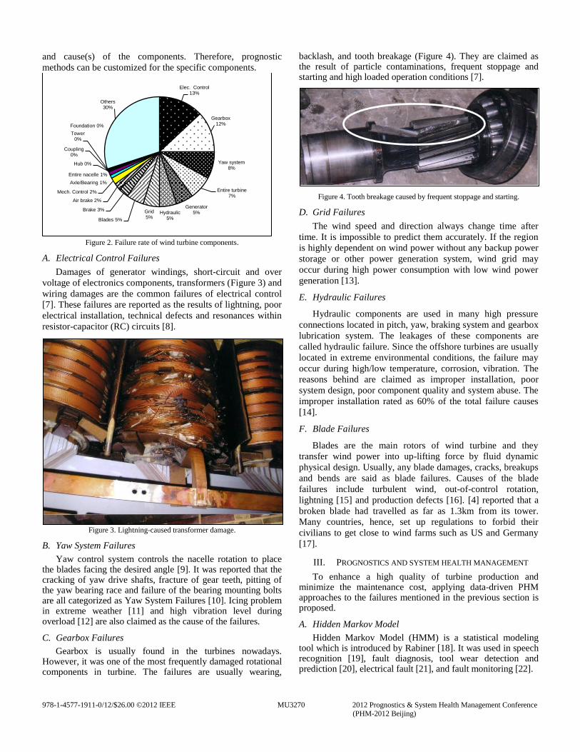
Electrical control, gearbox, yaw system, generator,
hydraulic, grid and blades are rated (60% of the total failures)
as the most common failure components of wind turbines
(>1.5MW) in the study of Danish turbines [6] (Figure 2).
Those challenges cause extra cost on emergency maintenance,
component screening, physical designs and so forth.
According to the failed components mentioned, a more details
are provided in the following with the failure mechanism(s)
Sensor
Data Sets
Historical
Database
Fault
Prognostics
Approaches
Remaining
Useful Life
System Health
Management
R&D
Improvement
978-1-4577-1911-0/12/$26.00 ©2012 IEEE MU3270 2012 Prognostics & System Health Management Conference (PHM-2012 Beijing)
and cause(s) of the components. Therefore, prognostic
methods can be customized for the specific components.
Figure 2. Failure rate of wind turbine components.
A. Electrical Control Failures
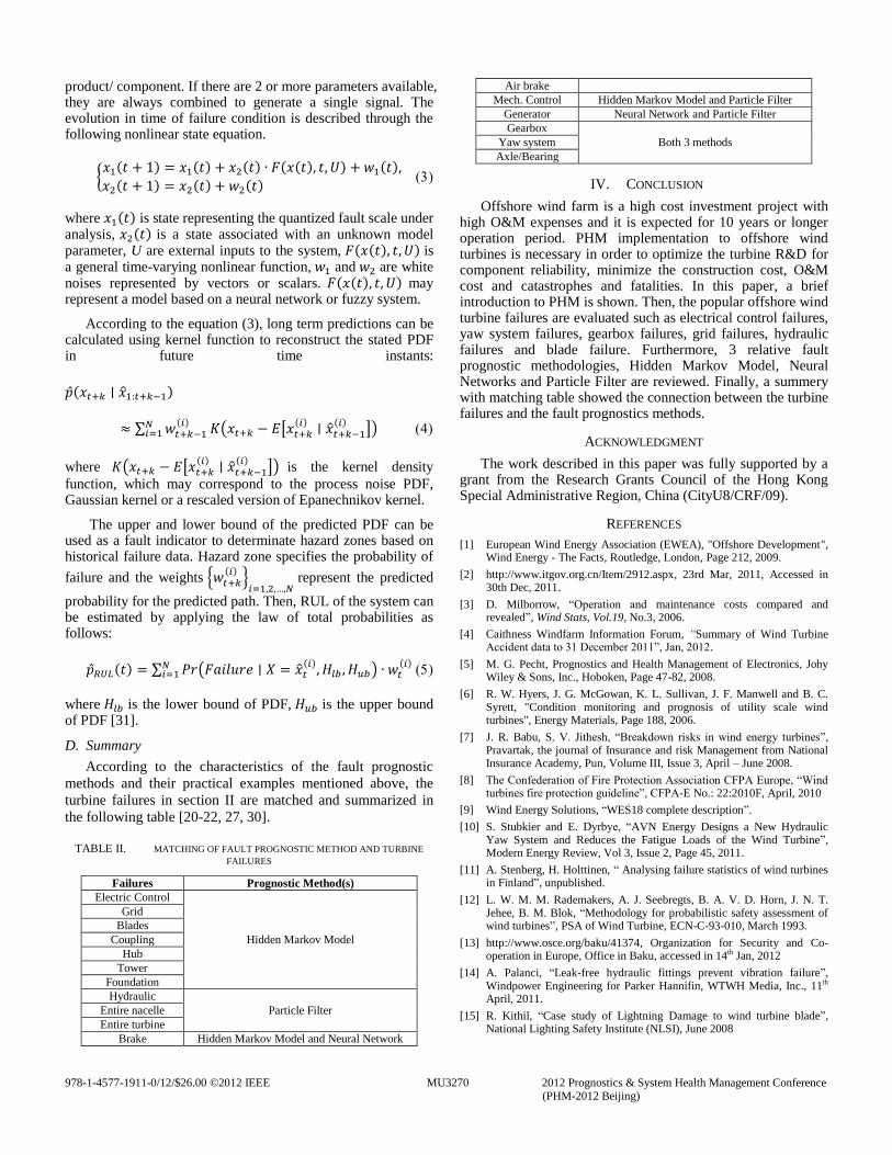
Damages of generator windings, short-circuit and over
voltage of electronics components, transformers (Figure 3) and
wiring damages are the common failures of electrical control
[7]. These failures are reported as the results of lightning, poor
electrical installation, technical defects and resonances within
resistor-capacitor (RC) circuits [8].
Figure 3. Lightning-caused transformer damage.
B. Yaw System Failures
Yaw control system controls the nacelle rotation to place the blades facing the desired angle [9]. It was reported that the cracking of yaw drive shafts, fracture of gear teeth, pitting of the yaw bearing race and failure of the bearing mounting bolts are all categorized as Yaw System Failures [10]. Icing problem in extreme weather [11] and high vibration level during overload [12] are also claimed as the cause of the failures.
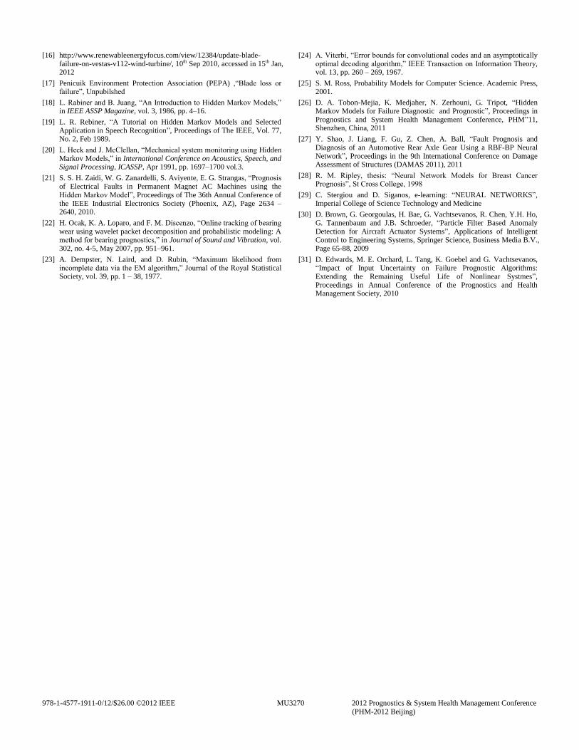
C. Gearbox Failures
Gearbox is usually found in the turbines nowadays. However, it was one of the most frequently damaged rotational components in turbine. The failures are usually wearing,
backlash, and tooth breakage (Figure 4). They are claimed as the result of particle contaminations, frequent stoppage and starting and high loaded operation conditions [7].
Figure 4. Tooth breakage caused by frequent stoppage and starting.
D. Grid Failures
The wind speed and direction always change time after
time. It is impossible to predict them accurately. If the region
is highly dependent on wind power without any backup power
storage or other power generation system, wind grid may
occur during high power consumption with low wind power
generation [13].
E. Hydraulic Failures
Hydraulic components are used in many high pressure
connections located in pitch, yaw, braking system and gearbox
lubrication system. The leakages of these components are
called hydraulic failure. Since the offshore turbines are usually
located in extreme environmental conditions, the failure may
occur during high/low temperature, corrosion, vibration. The
reasons behind are claimed as improper installation, poor
system design, poor component quality and system abuse. The
improper installation rated as 60% of the total failure causes
[14].
F. Blade Failures
Blades are the main rotors of wind turbine and they
transfer wind power into up-lifting force by fluid dynamic
physical design. Usually, any blade damages, cracks, breakups
and bends are said as blade failures. Causes of the blade
failures include turbulent wind, out-of-control rotation,
lightning [15] and production defects [16]. [4] reported that a
broken blade had travelled as far as 1.3km from its tower.
Many countries, hence, set up regulations to forbid their
civilians to get close to wind farms such as US and Germany
[17].
III. PROGNOSTICS AND SYSTEM HEALTH MANAGEMENT
To enhance a high quality of turbine production and minimize the maintenance cost, applying data-driven PHM approaches to the failures mentioned in the previous section is proposed.
A. Hidden Markov Model
Hidden Markov Model (HMM) is a statistical modeling tool which is introduced by Rabiner [18]. It was used in speech recognition [19], fault diagnosis, tool wear detection and prediction [20], electrical fault [21], and fault monitoring [22].
Elec. Control 13%
Gearbox 12%
Yaw system 8%
Entire turbine 7%
Generator 5% Hydraulic
5%
Grid 5%
Blades 5%
Brake 3%
Air brake 2%
Mech. Control 2%
Axle/Bearing 1%
Entire nacelle 1%
Coupling 0%
Hub 0%
Tower 0%
Foundation 0%
Others 30%

978-1-4577-1911-0/12/$26.00 ©2012 IEEE MU3270 2012 Prognostics & System Health Management Conference (PHM-2012 Beijing)
In general, HMM can be defined by the following parameters:
TABLE I. ELEMENTS DESCRIPTION OF HMM
Parameters Description
C Number of states/classes
π C x 1 initial state distribution vector where the ith element is
the probability of being in state i at time k = 0. p( = i)
A C x C state-transition matrix where the (i, j)th element is the
probability of being in state j at time k +1, given that it is in
state i at time k, p( = j| = i)
B
State-dependent observation density B. Its jth element is the
probability of observing at time k given the system is in
state j, bj( ) = p( | = j).
For convenience, the compact notation λ = {π, A, B} is used to indicate the complete parameter set of the model.
In prognostic application of HMM, Learning Phase and Exploitation Phase are included. In Learning Phase, the feature(s) from normal condition to failure situations are transformed into HMMs by Baum-Welch algorithm [23]. The HMMs then construct historical database for each failure. In Exploitation Phase, the on-line data are input to the model database to evaluate the health status of the current product or component by computing the probability ( ) where is defined as the observation sequence and is the online extracted features. Once the specific HMM is selected, Viterbi Algorithm [24] is used to find the state sequence ( ) and the last states sequence ( ) where l is the past observation factor and t is current time. Then, Chapman – Kolmogorov equation (1) is applied to estimate the health state after n iterations [25]. The Remaining Useful Life (RUL) is calculated when the predicted probability of being in the last state reaches a predefined limit in equation (2) [26].
( )
⇔ ( )
B. Neural Network
Neural Network (NN) is a mathematical model based on interconnected brain neuron structure. It can compose a large number of highly interconnected elements (neurons) working together to provide output(s) for problem solving. Besides PHM application, it was widely used in medical, marketing, electronic chip development, speech and vision recognition.
In the theory of NN, the neurons have 2 operation modes, training mode and using mode which are for ‗learning‘ purpose and ‗decision making‘ purpose, respectively. In using mode, if there are any inputs that are have not been learnt before, the ‗decision making‘ will follow the firing rules such as Hamming distance technique. NN is divided into 2 working principles. Feed-forward Network only allows signals travel in one way from inputs to outputs. It is extensively used in pattern recognition. Feedback networks enable feedbacks between neurons communications. The networks are dynamic which change continuously until the equilibrium state is reached. It can be extremely complicated but powerful.
Practically, NN is used in fault prognostic of axle gear [27].
Vibration signal of the axle gear is preprocessed by feature
extraction and then used as the precursor for prediction system.
There are 3 layers contained by Feed-forward network (Figure
5). The prediction is estimated by the previous outputs of the
network. For example, the network takes
as input to predict
at time instant t by Radial Basis
Function (RBF) Networks [28] [29] (Figure 6).
Figure 5. Feed-forward network layers.
Figure 6. Prediction framework of RBF Networks.
C. Particle Filter
Particle Filter (PF) is another method for fault prognostics applications. ‗Particle‘ means the unknown sample. The method aims to approximate the relevant distributions with particles and their associated weights. The state of Probability Density Function (PDF) is estimated which is used to predict the evolution in time of the fault indicator. It is useful to solve difficult nonlinear and/or non-Gaussian problems because of the use of Bayesian theory. Moreover, fewer samples are required to approximate the trend with acceptable accuracy. The short computation speed is also the advantage of the method. All these benefit in fault diagnostics and prognostics of complex dynamic systems like engines, gearboxes and bearings [30].
For the application of fault prognostics, there should be at least one parameter data set providing the health condition of
.
.
.
𝐶
𝐶
Hidden
layer
𝐶𝑘
Inputs
X
X
X𝑛
.
.
.
Outputs
y𝑚
y
.
.
.
Feedback for input mode
Prediction
y𝑡 𝑘
y𝑡
y𝑡
RBF
N
E
T
W
O
R
K
S
y𝑡 𝑘
��𝑡 . . .
Input
978-1-4577-1911-0/12/$26.00 ©2012 IEEE MU3270 2012 Prognostics & System Health Management Conference (PHM-2012 Beijing)
product/ component. If there are 2 or more parameters available, they are always combined to generate a single signal. The evolution in time of failure condition is described through the following nonlinear state equation.
{ ( ) ( ) ( ) ( ( ) ) ( )
( ) ( ) ( )
where ( ) is state representing the quantized fault scale under analysis, ( ) is a state associated with an unknown model parameter, U are external inputs to the system, ( ( ) ) is a general time-varying nonlinear function, and are white noises represented by vectors or scalars. ( ( ) ) may represent a model based on a neural network or fuzzy system.
According to the equation (3), long term predictions can be calculated using kernel function to reconstruct the stated PDF in future time instants:
( )
∑ ( )
( [ ( )
( ) ])
where ( [ ( )
( ) ]) is the kernel density
function, which may correspond to the process noise PDF, Gaussian kernel or a rescaled version of Epanechnikov kernel.
The upper and lower bound of the predicted PDF can be used as a fault indicator to determinate hazard zones based on historical failure data. Hazard zone specifies the probability of
failure and the weights { ( ) }
represent the predicted
probability for the predicted path. Then, RUL of the system can be estimated by applying the law of total probabilities as follows:
( ) ∑ ( ( ) )
( )
where is the lower bound of PDF, is the upper bound of PDF [31].
D. Summary
According to the characteristics of the fault prognostic
methods and their practical examples mentioned above, the
turbine failures in section II are matched and summarized in
the following table [20-22, 27, 30].
TABLE II. MATCHING OF FAULT PROGNOSTIC METHOD AND TURBINE
FAILURES
Failures Prognostic Method(s)
Electric Control
Hidden Markov Model
Grid
Blades
Coupling
Hub
Tower
Foundation
Hydraulic
Particle Filter Entire nacelle
Entire turbine
Brake Hidden Markov Model and Neural Network
Air brake
Mech. Control Hidden Markov Model and Particle Filter
Generator Neural Network and Particle Filter
Gearbox
Both 3 methods Yaw system
Axle/Bearing
IV. CONCLUSION
Offshore wind farm is a high cost investment project with high O&M expenses and it is expected for 10 years or longer operation period. PHM implementation to offshore wind turbines is necessary in order to optimize the turbine R&D for component reliability, minimize the construction cost, O&M cost and catastrophes and fatalities. In this paper, a brief introduction to PHM is shown. Then, the popular offshore wind turbine failures are evaluated such as electrical control failures, yaw system failures, gearbox failures, grid failures, hydraulic failures and blade failure. Furthermore, 3 relative fault prognostic methodologies, Hidden Markov Model, Neural Networks and Particle Filter are reviewed. Finally, a summery with matching table showed the connection between the turbine failures and the fault prognostics methods.
ACKNOWLEDGMENT
The work described in this paper was fully supported by a grant from the Research Grants Council of the Hong Kong Special Administrative Region, China (CityU8/CRF/09).
REFERENCES
[1] European Wind Energy Association (EWEA), "Offshore Development", Wind Energy - The Facts, Routledge, London, Page 212, 2009.
[2] http://www.itgov.org.cn/Item/2912.aspx, 23rd Mar, 2011, Accessed in 30th Dec, 2011.
[3] D. Milborrow, ―Operation and maintenance costs compared and revealed‖, Wind Stats, Vol.19, No.3, 2006.
[4] Caithness Windfarm Information Forum, “Summary of Wind Turbine Accident data to 31 December 2011‖, Jan, 2012.
[5] M. G. Pecht, Prognostics and Health Management of Electronics, Johy Wiley & Sons, Inc., Hoboken, Page 47-82, 2008.
[6] R. W. Hyers, J. G. McGowan, K. L. Sullivan, J. F. Manwell and B. C. Syrett, "Condition monitoring and prognosis of utility scale wind turbines", Energy Materials, Page 188, 2006.
[7] J. R. Babu, S. V. Jithesh, ―Breakdown risks in wind energy turbines‖, Pravartak, the journal of Insurance and risk Management from National Insurance Academy, Pun, Volume III, Issue 3, April – June 2008.
[8] The Confederation of Fire Protection Association CFPA Europe, ―Wind turbines fire protection guideline‖, CFPA-E No.: 22:2010F, April, 2010
[9] Wind Energy Solutions, ―WES18 complete description‖.
[10] S. Stubkier and E. Dyrbye, ―AVN Energy Designs a New Hydraulic Yaw System and Reduces the Fatigue Loads of the Wind Turbine‖, Modern Energy Review, Vol 3, Issue 2, Page 45, 2011.
[11] A. Stenberg, H. Holttinen, ― Analysing failure statistics of wind turbines in Finland‖, unpublished.
[12] L. W. M. M. Rademakers, A. J. Seebregts, B. A. V. D. Horn, J. N. T. Jehee, B. M. Blok, ―Methodology for probabilistic safety assessment of wind turbines‖, PSA of Wind Turbine, ECN-C-93-010, March 1993.
[13] http://www.osce.org/baku/41374, Organization for Security and Co-operation in Europe, Office in Baku, accessed in 14th Jan, 2012
[14] A. Palanci, ―Leak-free hydraulic fittings prevent vibration failure‖, Windpower Engineering for Parker Hannifin, WTWH Media, Inc., 11th April, 2011.
[15] R. Kithil, ―Case study of Lightning Damage to wind turbine blade‖, National Lighting Safety Institute (NLSI), June 2008
978-1-4577-1911-0/12/$26.00 ©2012 IEEE MU3270 2012 Prognostics & System Health Management Conference (PHM-2012 Beijing)
[16] http://www.renewableenergyfocus.com/view/12384/update-blade-failure-on-vestas-v112-wind-turbine/, 10th Sep 2010, accessed in 15th Jan, 2012
[17] Penicuik Environment Protection Association (PEPA) ,―Blade loss or failure‖, Unpubilshed
[18] L. Rabiner and B. Juang, ―An Introduction to Hidden Markov Models,‖ in IEEE ASSP Magazine, vol. 3, 1986, pp. 4–16.
[19] L. R. Rebiner, ―A Tutorial on Hidden Markov Models and Selected Application in Speech Recognition‖, Proceedings of The IEEE, Vol. 77, No. 2, Feb 1989.
[20] L. Heck and J. McClellan, ―Mechanical system monitoring using Hidden Markov Models,‖ in International Conference on Acoustics, Speech, and Signal Processing, ICASSP, Apr 1991, pp. 1697–1700 vol.3.
[21] S. S. H. Zaidi, W. G. Zanardelli, S. Aviyente, E. G. Strangas, ―Prognosis of Electrical Faults in Permanent Magnet AC Machines using the Hidden Markov Model‖, Proceedings of The 36th Annual Conference of the IEEE Industrial Electronics Society (Phoenix, AZ), Page 2634 – 2640, 2010.
[22] H. Ocak, K. A. Loparo, and F. M. Discenzo, ―Online tracking of bearing wear using wavelet packet decomposition and probabilistic modeling: A method for bearing prognostics,‖ in Journal of Sound and Vibration, vol. 302, no. 4-5, May 2007, pp. 951–961.
[23] A. Dempster, N. Laird, and D. Rubin, ―Maximum likelihood from incomplete data via the EM algorithm,‖ Journal of the Royal Statistical Society, vol. 39, pp. 1 – 38, 1977.
[24] A. Viterbi, ―Error bounds for convolutional codes and an asymptotically optimal decoding algorithm,‖ IEEE Transaction on Information Theory, vol. 13, pp. 260 – 269, 1967.
[25] S. M. Ross, Probability Models for Computer Science. Academic Press, 2001.
[26] D. A. Tobon-Mejia, K. Medjaher, N. Zerhouni, G. Tripot, ―Hidden Markov Models for Failure Diagnostic and Prognostic‖, Proceedings in Prognostics and System Health Management Conference, PHM‖11, Shenzhen, China, 2011
[27] Y. Shao, J. Liang, F. Gu, Z. Chen, A. Ball, ―Fault Prognosis and Diagnosis of an Automotive Rear Axle Gear Using a RBF-BP Neural Network‖, Proceedings in the 9th International Conference on Damage Assessment of Structures (DAMAS 2011), 2011
[28] R. M. Ripley, thesis: ―Neural Network Models for Breast Cancer Prognosis‖, St Cross College, 1998
[29] C. Stergiou and D. Siganos, e-learning: ―NEURAL NETWORKS‖, Imperial College of Science Technology and Medicine
[30] D. Brown, G. Georgoulas, H. Bae, G. Vachtsevanos, R. Chen, Y.H. Ho, G. Tannenbaum and J.B. Schroeder, ―Particle Filter Based Anomaly Detection for Aircraft Actuator Systems‖, Applications of Intelligent Control to Engineering Systems, Springer Science, Business Media B.V., Page 65-88, 2009
[31] D. Edwards, M. E. Orchard, L. Tang, K. Goebel and G. Vachtsevanos, ―Impact of Input Uncertainty on Failure Prognostic Algorithms: Extending the Remaining Useful Life of Nonlinear Systmes‖, Proceedings in Annual Conference of the Prognostics and Health Management Society, 2010
Related Documents