Review of Action Recognition and Detection Methods Soo Min Kang and Richard P. Wildes Department of Electrical Engineering and Computer Science York University Toronto, Ontario Canada arXiv:1610.06906v2 [cs.CV] 1 Nov 2016

Welcome message from author
This document is posted to help you gain knowledge. Please leave a comment to let me know what you think about it! Share it to your friends and learn new things together.
Transcript
Review ofAction Recognition and Detection
Methods
Soo Min Kang and Richard P. Wildes
Department of Electrical Engineering and Computer Science
York University
Toronto, Ontario
Canada
arX
iv:1
610.
0690
6v2
[cs
.CV
] 1
Nov
201
6
Abstract
In computer vision, action recognition refers to the act of classifying an action thatis present in a given video and action detection involves locating actions of interestin space and/or time. Videos, which contain photometric information (e.g. RGB,intensity values) in a lattice structure, contain information that can assist in iden-tifying the action that has been imaged. The process of action recognition anddetection often begins with extracting useful features and encoding them to ensurethat the features are specific to serve the task of action recognition and detection.Encoded features are then processed through a classifier to identify the action classand their spatial and/or temporal locations. In this report, a thorough review ofvarious action recognition and detection algorithms in computer vision is providedby analyzing the two-step process of a typical action recognition and detection al-gorithm: (i) extraction and encoding of features, and (ii) classifying features intoaction classes. In efforts to ensure that computer vision-based algorithms reach thecapabilities that humans have of identifying actions irrespective of various nuisancevariables that may be present within the field of view, the state-of-the-art methodsare reviewed and some remaining problems are addressed in the final chapter.
1

Contents
1 Introduction 4
2 Benchmark Datasets 62.1 Testing Protocol . . . . . . . . . . . . . . . . . . . . . . . . . . . . . 62.2 Static Background . . . . . . . . . . . . . . . . . . . . . . . . . . . . 7
2.2.1 The KTH Dataset . . . . . . . . . . . . . . . . . . . . . . . . 82.2.2 The Weizmann Dataset . . . . . . . . . . . . . . . . . . . . . . 82.2.3 MPII Cooking Activities Dataset . . . . . . . . . . . . . . . . 92.2.4 Discussion . . . . . . . . . . . . . . . . . . . . . . . . . . . . . 11
2.3 Dynamic Background . . . . . . . . . . . . . . . . . . . . . . . . . . . 112.3.1 The CMU Crowded Videos Dataset . . . . . . . . . . . . . . . 112.3.2 The MSR Action Dataset I, II . . . . . . . . . . . . . . . . . . 13
2.4 Activities . . . . . . . . . . . . . . . . . . . . . . . . . . . . . . . . . 152.4.1 The UC Berkeley Dataset . . . . . . . . . . . . . . . . . . . . 152.4.2 UCF Sports Dataset . . . . . . . . . . . . . . . . . . . . . . . 162.4.3 The Olympic Dataset . . . . . . . . . . . . . . . . . . . . . . . 172.4.4 Sports-1M . . . . . . . . . . . . . . . . . . . . . . . . . . . . . 192.4.5 Discussion . . . . . . . . . . . . . . . . . . . . . . . . . . . . . 20
2.5 Movies . . . . . . . . . . . . . . . . . . . . . . . . . . . . . . . . . . . 202.5.1 Hollywood1 . . . . . . . . . . . . . . . . . . . . . . . . . . . . 212.5.2 Hollywood2 . . . . . . . . . . . . . . . . . . . . . . . . . . . . 212.5.3 Discussion . . . . . . . . . . . . . . . . . . . . . . . . . . . . . 21
2.6 Home Videos . . . . . . . . . . . . . . . . . . . . . . . . . . . . . . . 222.6.1 UCF11 (YouTube Action), UCF50, and UCF101 . . . . . . . . 232.6.2 ActivityNet . . . . . . . . . . . . . . . . . . . . . . . . . . . . 242.6.3 Discussion . . . . . . . . . . . . . . . . . . . . . . . . . . . . . 28
2.7 The Human Motion Databases . . . . . . . . . . . . . . . . . . . . . . 282.7.1 HMDB51 . . . . . . . . . . . . . . . . . . . . . . . . . . . . . 282.7.2 J-HMDB . . . . . . . . . . . . . . . . . . . . . . . . . . . . . . 33
2.8 Challenges . . . . . . . . . . . . . . . . . . . . . . . . . . . . . . . . . 332.8.1 THUMOS’ 13 . . . . . . . . . . . . . . . . . . . . . . . . . . . 332.8.2 THUMOS’ 14 . . . . . . . . . . . . . . . . . . . . . . . . . . . 342.8.3 THUMOS’ 15 . . . . . . . . . . . . . . . . . . . . . . . . . . . 372.8.4 ActivityNet Challenge . . . . . . . . . . . . . . . . . . . . . . 382.8.5 Final Remarks on the Challenges . . . . . . . . . . . . . . . . 39
2
CONTENTS CONTENTS
2.9 Summary . . . . . . . . . . . . . . . . . . . . . . . . . . . . . . . . . 39
3 Image Representation 433.1 Feature Extraction . . . . . . . . . . . . . . . . . . . . . . . . . . . . 43
3.1.1 Sampling Methods . . . . . . . . . . . . . . . . . . . . . . . . 443.1.2 Feature Descriptors . . . . . . . . . . . . . . . . . . . . . . . . 49
3.2 Encoding Methods . . . . . . . . . . . . . . . . . . . . . . . . . . . . 633.2.1 Codebook Generation . . . . . . . . . . . . . . . . . . . . . . 633.2.2 Assignment Methods . . . . . . . . . . . . . . . . . . . . . . . 663.2.3 Pooling and Normalization . . . . . . . . . . . . . . . . . . . . 713.2.4 Discussion on Encoding Methods . . . . . . . . . . . . . . . . 74
3.3 Feature Post-processing . . . . . . . . . . . . . . . . . . . . . . . . . . 763.4 Final Remarks . . . . . . . . . . . . . . . . . . . . . . . . . . . . . . . 77
4 Classification 784.1 Comparison Metrics . . . . . . . . . . . . . . . . . . . . . . . . . . . 784.2 Deterministic Models . . . . . . . . . . . . . . . . . . . . . . . . . . . 83
4.2.1 Lazy Learners . . . . . . . . . . . . . . . . . . . . . . . . . . . 844.2.2 Eager Learners . . . . . . . . . . . . . . . . . . . . . . . . . . 85
4.3 Probabilistic Models . . . . . . . . . . . . . . . . . . . . . . . . . . . 874.3.1 General Classifiers . . . . . . . . . . . . . . . . . . . . . . . . 874.3.2 Temporal State-Space Classifiers . . . . . . . . . . . . . . . . 92
4.4 Final Remarks . . . . . . . . . . . . . . . . . . . . . . . . . . . . . . . 96
5 Current Status 975.1 Current Trends . . . . . . . . . . . . . . . . . . . . . . . . . . . . . . 975.2 Open Problems . . . . . . . . . . . . . . . . . . . . . . . . . . . . . . 101
Appendix A Related Fields 104
References 107
3

Chapter 1
Introduction
Videos have become a vital component of our lives as it contains important informa-tion about the world. Its information has served humans in various domains: fromsecurity to robotics to entertainment and many more. The practicality of videoshave led to immense advancements for video recording, viewing, and distribution.One major drawback of such availability, however, is the overwhelming amount ofvideos that are produced for viewing and analysis by humans. An alternative tothis tedious task is to use machines to automatically extract useful information ina video. Consequently, detecting and localizing human actions has been a topic ofhigh interest in computer vision for many years.
Various terms (e.g. action recognition, action spotting, event recognition, etc.)have been coined to describe similar tasks. Thus, it is important that we definethe terms precisely to avoid any misunderstandings. First, we must distinguish thedifference between an action and an event. An action refers to motion created bythe human body, which may or may not be cyclic. An event is composed of mul-tiple primitive actions and can involve more than a single individual. While ‘run’and ‘jump’ are some examples of cyclic and non-cyclic actions, respectively, ‘hurdle’would be an example of an event since it can be broken down into two primitiveactions: ‘run’ and ‘jump’. Second, we must identify the similarities and differencesbetween the following terms: recognition, classification, detection, localization, andspotting. Action recognition and classification are terms that are used interchange-ably to describe the act of categorizing an action in a clip to one of the pre-defined setof actions. Action detection, localization, and spotting are also synonymous terms,which aim to determine the action and its location (in space and/or time). In thissurvey, we focus on actions rather than events, and both recognition and detectionalgorithms will be studied.
With the emergence of wearable cameras (e.g. GoPro and Google Glass), first-person action recognition has also been of interest to many in the computer vi-sion community. First- and third-person action recognition algorithms are two veryclosely related tasks. However, there is a significant difference between the two.First-person action recognition involves determining the action executed by the per-
4
CHAPTER 1. INTRODUCTION
son wearing the camera from an egocentric viewpoint. Third-person action recog-nition, on the other hand, involves determining the action executed by a person ascaptured by someone other than the actor. This difference results in contrastingdatasets, actions of interest, and viewpoints. Thus, we emphasize here that thispaper primarily reviews third-person action recognition and detection algorithms.First-person action recognition algorithms along with a select few other related fieldsof action recognition and detection are briefed in Appendix A.
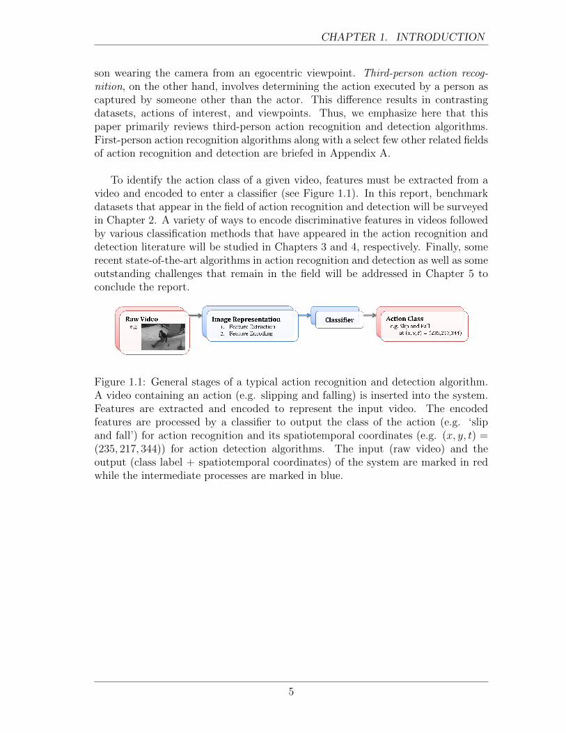
To identify the action class of a given video, features must be extracted from avideo and encoded to enter a classifier (see Figure 1.1). In this report, benchmarkdatasets that appear in the field of action recognition and detection will be surveyedin Chapter 2. A variety of ways to encode discriminative features in videos followedby various classification methods that have appeared in the action recognition anddetection literature will be studied in Chapters 3 and 4, respectively. Finally, somerecent state-of-the-art algorithms in action recognition and detection as well as someoutstanding challenges that remain in the field will be addressed in Chapter 5 toconclude the report.
Figure 1.1: General stages of a typical action recognition and detection algorithm.A video containing an action (e.g. slipping and falling) is inserted into the system.Features are extracted and encoded to represent the input video. The encodedfeatures are processed by a classifier to output the class of the action (e.g. ‘slipand fall’) for action recognition and its spatiotemporal coordinates (e.g. (x, y, t) =(235, 217, 344)) for action detection algorithms. The input (raw video) and theoutput (class label + spatiotemporal coordinates) of the system are marked in redwhile the intermediate processes are marked in blue.
5

Chapter 2
Benchmark Datasets
With the growing popularity of various action recognition and detection algorithms,it is important to understand the comparative and absolute strengths and weaknessesof each approach. One of the most just ways to draw comparisons is to quantita-tively evaluate each approach on the same database with the same protocol. Thus,it is important to survey the commonly used datasets and their key features to un-derstand the capabilities and limitations of each tested approach [1, 21, 95]. In thischapter, some common testing protocols will be reviewed, benchmark datasets usedfor evaluation in subsequent chapters will be studied, then a quantitative summaryof the datasets will follow. The datasets have been categorized by some commonfeatures that they share and a thorough analysis was conducted for each datasetby surveying their key characteristics, quantitative summary including the num-ber of actors, actions, and conditions, video specifications (e.g. spatial resolution,video duration, frame rate), test protocols, and its intended use (recognition and/ordetection).
2.1 Testing Protocol
To make a fair comparison between algorithms, it is very important to test themunder the same protocol. First, the training, validation, and test data that areused to evaluate these algorithms must be consistent. As its name suggests, thepurpose of a training set is to train the classifier (i.e. to optimize the parametersof the classifier (e.g. weights in neural networks)). The validation set, which isoptional, is comprised of data distinct from those in the training set. It is used tomake adjustments on the selected model such that the algorithm can perform wellon both the training and the validation set. A validation set often is used to findthe most optimal hyperparameters (e.g. number of hidden units, length of training,training rate in neural networks) for the model. The model that performs the beston the training and validation sets is finally assessed using the test set to measurethe performance of the overall system [31]. Separating a dataset into three disjointsets (training, validation, and testing) allows researchers to tune their system andestimate the error simultaneously.
6

2.2 Static Background CHAPTER 2. BENCHMARK DATASETS
Second, the method of splitting a dataset into training, validation, and testmust be uniform. There are three general ways to divide a set [31]: (i) using apre-defined split, (ii) through n-fold cross-validation, and (iii) through leave-one-out cross-validation. The pre-defined split separates the dataset into two (or three)uneven components: training and testing (and validation), which is specified by theauthors of the dataset. The n-fold cross-validation divides the dataset into n mu-tually exclusive equal-sized folds. Videos in n− 1 folds, which is approximately n−1
n
videos of the entire set, are used for training, and the remaining fold, approximately1n
videos, is used for testing. This process is repeated n times such that all clips areused once for testing. The average error rate of each fold is the estimated error rateof the classifier. The leave-one-out cross-validation is a special instance of cross-validation, where each removed sequence is compared to the remaining sequences.Leave-one-out is computationally expensive, but it determines the most accurateestimate of a classifier’s error rate.
Third, a single quantitative measure should be used for comparison. To evaluatehow an action recognition algorithm performs with respect to each action class, aninterpolated average precision (AP) can be used. AP is defined as:
AP (c) =
∑nk=1 (P (k)× rel(k))∑n
k=1 rel(k)(2.1)
for test class c, where n is the total number of videos, P (k) is the precision at cutoffk of the list, and rel(k) is an indicator function which equals 1 if the video rankedk is a true positive and 0 otherwise. The denominator in (2.1) represents the totalnumber of true positives in the list. The overall performance of the system can beevaluated using the mean average precision (mAP) measure, which is defined as:
mAP =1
C
C∑c=1
AP (c), (2.2)
where C is the total number of test classes (i.e. C = 101 for UCF101). To de-termine whether the prediction should be considered a true or false positive for adetection algorithm, a threshold value can be associated with the intersection-over-union (IoU) to accept or reject a detected result. That is, if o denotes IoU betweenthe predicted location, Lp, and the ground truth location, Lgt, then o can be writtenmathematically as:
o =Lp ∩ LgtLp ∪ Lgt
, (2.3)
and Lp is considered correct if o ≥ κ for some constant κ.
2.2 Static Camera with Clean Background
One of the earliest goals in action recognition was to classify the action of a singleindividual in a video given a set of actions. Thus, a benchmark dataset containing
7

2.2 Static Background CHAPTER 2. BENCHMARK DATASETS
a heterogeneous set of actions with systematic variations of parameters was in greatdemand. The KTH and Weizmann datasets met these requirements and becametwo of the earliest standard datasets of which to test action recognition algorithms.These datasets share a common characteristic of actors performing the actions infront of a simple background recorded with a static camera. Here, KTH, Weizmann,and the more recent MPII Cooking Activities datasets will be surveyed.
2.2.1 The KTH Dataset
The efforts to create a non-trivial and publicly available dataset for action recog-nition was initiated at the KTH Royal Institute of Technology in 2004. The KTHdataset [148] is one of the most standard datasets, which contains six actions: walk,jog, run, box, hand-wave, and hand clap (see Figure 2.1). To account for perfor-mance nuance, each action is performed by 25 different individuals, and the settingis systematically altered for each action per actor. Setting variations include: out-door (s1), outdoor with scale variation (s2), outdoor with different clothes (s3), andindoor (s4). These variations test the ability of each algorithm to identify actionsindependent of the background, appearance of the actors, and the scale of the actors.
The KTH dataset contains 6 actions performed by 25 individuals in 4 differentsettings (6 actions × 25 actors × 4 settings) resulting in a total of 600 clips1.Each clip contains multiple instances of a single action and is recorded on a staticcamera with a frame rate of 25 frames per second (fps). The videos were down-sampled to have a spatial resolution of 160×120 pixels and each clip ranges from8 seconds (204 frames) to 59 seconds (1492 frames) averaging 18.9 seconds. Thetest protocol of the KTH dataset divides the videos into training, validation, andtest sets, which contains 8, 8, and 9 actors, respectively. The dataset is useful forthe task of recognition and temporal detection, as the ground truth indicates whenspecific actions occur but not where (the location).
2.2.2 The Weizmann Dataset
The following year after the KTH dataset was released, the Weizmann Actions asSpace-Time Shapes dataset (or the Weizmann dataset [14]) at the Weizmann Insti-tute of Science in the Department of Computer Science and Applied Mathematics inIsrael also became available in the field of action recognition. The Weizmann datasetcontains more actions than the KTH (bend, wave one hand, wave two hands, jump-ing jack, jump in place on two legs, jump forward on two legs, walk, run, skip, andgallop sideways (see Figure 2.2)), but each action is performed by fewer individuals.Nevertheless, performance by nine individuals is enough to take into considerationthe nuance between individuals. The actors repeat most actions, namely skip, jump,run, gallop sideways, walk, in opposite directions to account for the asymmetry ofthese actions. Like the KTH dataset, the videos in this dataset are recorded using
1A clip of person 13 performing hand clap in the outdoor with different clothes (s3) setting ismissing in the KTH dataset resulting in a total of 599 clips instead of 600.
8

2.2 Static Background CHAPTER 2. BENCHMARK DATASETS
Figure 2.1: The KTH Dataset. The KTH dataset contains six different actions(left-to-right): walk, jog, run, box, hand-wave, and hand clap; taken at four dif-ferent settings (top-to-bottom): outdoor (s1), outdoor with scale variation (s2),outdoor with different clothes (s3), and indoor (s4). Redrawn from [148].
a static camera on a uniform background. The actors move horizontally across theframe, maintaining the consistency in the size of the actor as they perform eachaction.
The Weizmann dataset contains 10 actions performed by 9 individuals (10 actions× 9 actors) resulting in a total of 90 clips2. Each clip contains multiple instancesof a single action. Each clip was recorded on a static camera with 50 fps, but hasbeen deinterlaced to 25 fps. The videos have a spatial resolution of 180×144 pixelsand each clip ranges from 1 second (36 frames) to 5 seconds (125 frames) averaging3.66 seconds. The recommended testing protocol for using the Weizmann dataset isto perform a leave-one-out procedure. Although the intended use of the dataset isfor action recognition, it is also useful for the task of detection, as the ground truthare silhouette masks, which can be applied to extract both spatial and temporalinformation of the action.
2.2.3 MPII Cooking Activities Dataset
A group from the Max Planck Institute for Informatics (MPII) compiled the MPIICooking Activities [141] and its extension MPII Cooking 2 [142] datasets, whichconsist of actions related to cooking. The goal of these datasets is to distinguishbetween fine-actions, which is a very challenging task since there is high intra-class
2Select actions (run, skip, and walk) by one of the individuals, Lena, are split into two clipsresulting in 10 clips per action instead of 9. Thus, there are a total of 93 clips instead of 90.
9

2.2 Static Background CHAPTER 2. BENCHMARK DATASETS
Figure 2.2: The Weizmann Dataset. The Weizmann dataset contains ten actions(left-to-right, top-to-bottom): bend, jump in place on two legs (P-jump), wave twohands (wave2), run, jump forward on two legs (jump), jumping jack (jacks), walk,wave one hand (wave1), skip, and gallop sideways (side). Redrawn from [14].
variation (e.g. peeling a carrot vs. peeling a pineapple) and low inter-class varia-tion (e.g. mixing vs. stirring or dicing vs. slicing). Participants, whose cookingskills range from beginner to amateur chefs, were instructed to cook one to six ofpre-defined dishes (e.g. fruit salad) for the MPII Cooking dataset. The individualswere not given a specific recipe to follow. As a result, each individual used differentingredients to prepare each dish and very dissimilar videos were obtained. For eachcooking video, actions (e.g. cut, peel) were annotated. A list of the 14 (and 59additional) pre-defined dishes and the annotated 65 (and 67) actions for the MPIICooking Activities (and MPII Cooking 2) dataset are listed in Table 2.1 (and 2.2).
The MPII Cooking Activity dataset contains 12 subjects, where 7 of the subjectsare used to perform leave-one-out cross-validation. That is, one of the subjects areremoved from training, and the other 11 are used and this process is repeated 7 times.The MPII Cooking 2 dataset contains 30 subjects in 273 videos. The dataset is splitinto 201 training, 17 validation, and 42 testing with no overlap between the subjects.The training, validation, and test splits do not sum to the full dataset because forall composite actions in the testing set, the authors ensured that there were at least3 training and validation videos from the same actor. Since some subjects hadless than 3 training or validation videos, some test subjects were not used. Eachvideo was recorded on a mounted camera attached to the ceiling, recording the actorworking at the counter from the frontal view. The videos in both datasets have aspatial resolution of 1624× 1224 with a frame rate of 29.4 fps, and the duration ofthe videos in the MPII Cooking 2 dataset ranges from 2 minutes and 44 secondsto 24 minutes and 34 seconds for a total of 8 hours and 19 minutes. Both datasetsare useful for the task of action recognition as well as detection. Average precision(AP) is computed to compare per class results and mean average precision is usedto report the overall performance of the algorithm on the datasets. The mid-point
10

2.3 Dynamic Background CHAPTER 2. BENCHMARK DATASETS
criterion is used to decide the correctness of the detection. That is, if the mid-pointof the detection is within the ground truth, then it is considered correct.
2.2.4 Discussion
The KTH and Weizmann datasets set a good stepping stone for the field of actionrecognition through their heterogeneous selection of actions and systematic varia-tions in its parameters. The controlled settings, such as absence of occlusion andclutter, limited variations in illumination and camera motion, allow these datasetsto be ideal for standard testing. Unfortunately, good performance on the KTH andWeizmann datasets does not suffice to determine the algorithm’s proficiency in real-world videos due to the richness and complexity of the videos in the real-world. Infact, while state-of-the-art action recognition algorithms routinely achieve greaterthan 90% recognition accuracy on these datasets, they perform far less well on themore naturalistic datasets that are to be introduced in the remainder of this chap-ter. For this reason, strong performance on the KTH and Weizmann datasets is nolonger of much interest in the field.
The MPII Cooking 2 dataset shifts the focus of recognizing full-body movements(e.g. run, jump) to classifying actions with small motions. This fine-grained catego-rization can assist in differentiating visually similar activities that frequently occurin daily living (e.g. hug vs. hold someone and throw in garbage vs. put in drawer).The MPII Cooking 2 dataset also provides data for the often neglected but morechallenging and realistic temporal detection task.
2.3 Still Camera with Background Motion
To accommodate the lack of naturalistic settings in the KTH and Weizmann datasets,in particular the clean nature of the background, the next step was to test algorithmson videos with a dynamic background. In this section, the CMU Crowded Videosdataset and the MSR Action Dataset I, II, which contain videos with backgroundmotion and clutter will be examined. Dynamic background was obtained by record-ing videos in environments with moving cars and people.
2.3.1 The CMU Crowded Videos Dataset
A group from Carnegie Mellon University (CMU) was one of the first to assemblea dataset, called the CMU Crowded Videos Dataset [76], for the action recognitionand detection tasks that contain background motion. The CMU Crowded VideosDataset focuses on five actions: pick-up, one-hand wave, push button, jumping jack,and two-hand wave. As many of the actions in the CMU Crowded Video datasetoverlap those in the KTH and Weizmann, it was also one of the first cross-datasetsthat appeared in the field. That is, one of the training videos that is supplied in
11

2.3 Dynamic Background CHAPTER 2. BENCHMARK DATASETS
Dishes sandwich, salad, fried potatoes, potato pancake, omelet, soup, pizza,casserole, mashed potato, snack plate, cake, fruit salad, cold drink, andhot drink
Actions background activity, change temperature, cut apart, cut dice, cut in,cut off ends, cut out inside, cut slices, cut stripes, dry, fill water fromtap, grate, put on lid, remove lid, mix, move from X to Y, open egg,open tin, open/close cupboard, open/close drawer, open/close fridge,open/close oven, package X, peel, plug in/out, pour, pull out, puree, putin bowl, put in pan/pot, put on bread/dough, put on cutting-board, puton plate, read, remove from package, rip open, scratch off, screw close,screw open, shake, smell, spice, spread, squeeze, stamp, stir, strew, takeand put in cupboard, take and put in drawer, take and put in fridge,take and put in oven, take and put in spice holder, take ingredientapart, take out from cupboard, take out from drawer, take out fromfridge, take out from oven, take out from spice holder, taste, throw ingarbage, unroll dough, wash hands, wash objects, whisk, and wipe clean
Table 2.1: MPII Cooking Dataset [141]. 14 pre-defined dishes and 65 annotatedactions are listed.
Dishes cooking pasta, juicing {lime, orange}, making {coffee, hot dog, tea},pouring beer, preparing {asparagus, avocado, borad beans, broccoli andcauliflower, broccoli, carrot and potatoes, carrots, cauliflower, chilli,cucumber, figs, garlic, ginger, herbs, kiwi, leeks, mango, onion, orange,peach, peas, pepper, pineapple, plum, pomegranate, potatoes, scrambledeggs, spinach, spinach and leeks}, separating egg, sharpening knives,slicing loaf of bread, using {microplane grater, pestle and mortar, speedpeeler, toaster, tongs}, zesting lemon
Actions add, arrange, change temperature, chop, clean, close, cut apart, cutdice, cut off ends, cut out inside, cut stripes, cut, dry, enter, fill, gather,grate, hang, mix, move, open close, open egg, open tin, open, package,peel, plug, pour, pull apart, pull up, pull, puree, purge, push down, putin, put lid, put on, read, remove from package, rip open, scratch off,screw close, screw open, shake, shape, slice, smell, spice, spread, squeeze,stamp, stir, strew, take apart, take lid, take out, tap, taste, test tem-perature, throw in garbage, turn off, turn on, turn over, unplug, wash,whip, wring out
Table 2.2: MPII Cooking 2 Dataset [142]. Additional 41 dishes that were added tothe MPII Cooking 2 dataset and 67 annotated actions are listed. The dishes thatwere added are slightly shorter and simpler than the dishes in the MPII Cookingdataset.
12
2.3 Dynamic Background CHAPTER 2. BENCHMARK DATASETS
this dataset is the exact same video as the two-hand wave in the KTH dataset.
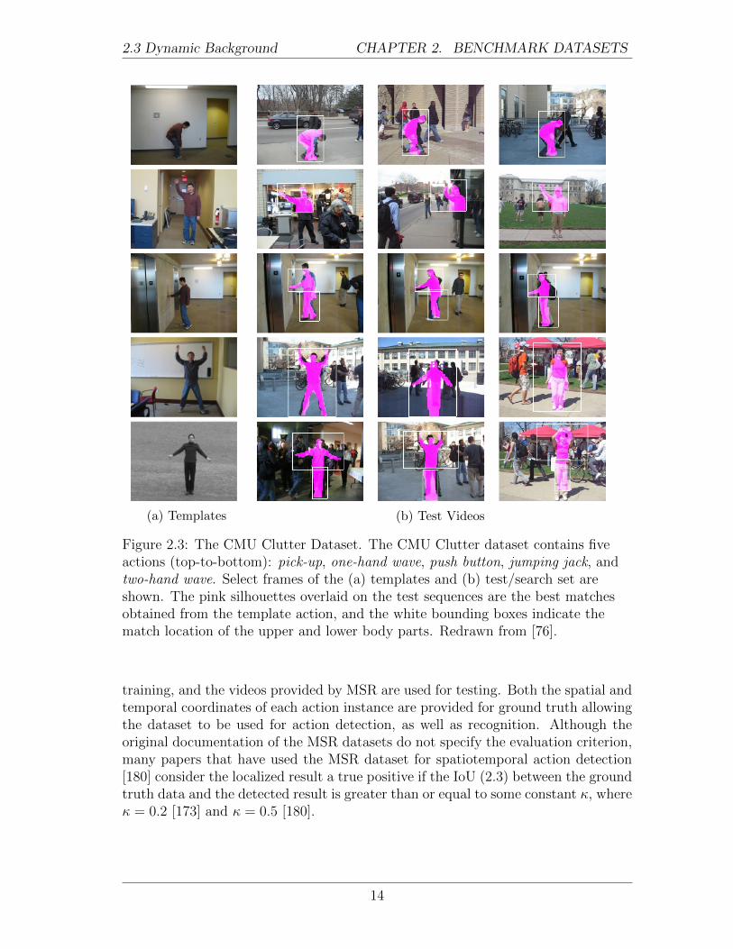
The CMU Crowded Videos dataset contains 5 training videos for each actionand 48 test videos. Each training video is performed by a single individual on astatic background. The test videos contain three to six individuals different fromthose in the training set, and contains one to six instances of any three actions inno particular order (see Figure 2.3). All videos, training and testing, have beenscaled such that the spatial resolution of each video is 120 × 160. All videos havea frame rate of 30 fps, except the two handed wave, which has a frame rate of 25fps. The test videos range from 5 to 37 seconds (166 to 1115 frames). The authorsprovide spatial and temporal coordinates (x, y, height, width, start, and end frames)for specified actions as ground truth, giving researchers the option to evaluate theability of an algorithm to recognize and detect actions of interest. The detectedaction is considered a true positive if there is greater than 50% overlap (in spaceand time) with the labelled action.
2.3.2 The MSR Action Dataset I, II
The Microsoft Research Group (MSR) also created action recognition datasets, re-ferred to as the MSR Action dataset I [219] and MSR Action dataset II [20], whereII is a direct extension of I. These were made available in 2009 and 2010, respectively.Similar to the CMU Crowded dataset, the purpose of the MSR Action dataset con-struction was to obtain videos that contain cluttered and/or dynamic backgrounds[20, 219]. The datasets were assembled to detect 3 actions: clap, (two-)hand wave,and boxing. The MSR Action datasets are instances of a full cross-dataset3. Thatis, to use the test videos in the MSR datasets, the actions must be trained using thevideos in the KTH dataset. Each test sequence contains multiple actions, varies inthe number of participants performing the action, the number of individuals in thevideo, and the number of actions that occur simultaneously. Some sequences containactions performed by a single individual, some performed by different individuals ata time, and some performed by two individuals simultaneously.
The MSR Action dataset I contains 24 instances of box, 24 instances of a two-hand wave, and 14 instances of clap, tallying 62 instances in total for 16 videosequences. The MSR Action dataset II, on the other hand, contains 81, 71, and 51instances of box, wave, and clap, respectively, to sum up to a total of 203 instances ofthe three actions in a set of 54 videos. All videos in the MSR Action dataset I have aframe rate of 15 fps, and ranges from 32 to 76 seconds (480 to 1149 frames). Videosin the MSR Action dataset II, on the other hand, have varying frame rates rangingfrom 14 to 15 fps, and are 21 to 85 seconds (321 to 1284 frames) long. All videosin both the MSR Action dataset I and II have a spatial resolution of 240 × 320,and are filmed using a static camera. As mentioned before, the videos from theKTH dataset that correspond to the three actions: box, wave, and clap are used for
3Cross-datasets allow researchers to develop general algorithms deviating from action- ordataset-specific recognition algorithms.
13
2.3 Dynamic Background CHAPTER 2. BENCHMARK DATASETS
(a) Templates (b) Test Videos
Figure 2.3: The CMU Clutter Dataset. The CMU Clutter dataset contains fiveactions (top-to-bottom): pick-up, one-hand wave, push button, jumping jack, andtwo-hand wave. Select frames of the (a) templates and (b) test/search set areshown. The pink silhouettes overlaid on the test sequences are the best matchesobtained from the template action, and the white bounding boxes indicate thematch location of the upper and lower body parts. Redrawn from [76].
training, and the videos provided by MSR are used for testing. Both the spatial andtemporal coordinates of each action instance are provided for ground truth allowingthe dataset to be used for action detection, as well as recognition. Although theoriginal documentation of the MSR datasets do not specify the evaluation criterion,many papers that have used the MSR dataset for spatiotemporal action detection[180] consider the localized result a true positive if the IoU (2.3) between the groundtruth data and the detected result is greater than or equal to some constant κ, whereκ = 0.2 [173] and κ = 0.5 [180].
14

2.4 Activities CHAPTER 2. BENCHMARK DATASETS
Figure 2.4: KTH vs. MSR. Comparison between the KTH dataset (top row) andthe MSR dataset (bottom row) for actions boxing, two-hand wave, and clap (left-to-right). Redrawn from [20].
2.4 Action Recognition in Activity Videos
Along with many other videos, there are also plentiful sports and performance videosonline that require categorization for accessible browsing and organization. A groupfrom UC Berkeley collected videos from various sources to gather clips that fre-quently appear in ballet, tennis, and soccer [34]. This marked the beginning stagesof collecting videos from multiple angles and moving cameras. In the following sec-tion, four activity-related action recognition/detection datasets will be introduced:the UC Berkeley Sports Dataset, the UCF Sports dataset, the Olympic Dataset,and Sports-1M.
2.4.1 The UC Berkeley Dataset
The UC Berkeley dataset consists of videos from three types of activities: ballet,tennis, and soccer. The ballet videos were collected from instructional videos, whichcontain four professional ballet dancers (two ballerinas and two ballerinos) perform-ing mostly standard ballet moves. 16 ballet actions (standard moves) were chosenfor the task of action detection: second position plies, first position plies, releve,down from releve, point toe and step right, point toe and step left, arms first posi-tion to second position, rotate arms in second position, degage, arms first positionforward and out to second position, arms circle, arms second to high fifth, arms highfifth to first, port de dras, right arm from high fifth to right, and port de bra flowyarms (refer to Figure 2.5a to view select frames of each action). Each action waschoreographed and all videos were filmed with a stationary camera.
Two amateur tennis players playing tennis outdoors were recorded to gather
15
2.4 Activities CHAPTER 2. BENCHMARK DATASETS
videos for the tennis portion of the dataset. Videos were filmed on different days atdifferent courts with slightly different camera positions to test variation in settingand perspective. Six actions were selected to complete the task of action recognitionin tennis videos, which are: swing, move left, move right, move left and swing, moveright and swing, and stand (refer to Figure 2.5b to see select frames from the tennisset).
The videos for the soccer component were gathered from footages of the WorldCup games. Among many angles that were available, only wide-angle shots of theplaying field were collected. This angle forces each human figure to span 30 × 30pixels on average, which is coarse for a video with a resolution of 640× 480. Unlikethe ballet and tennis videos, there is camera motion in the videos, a new challengein the field of action recognition that has yet to have been introduced. The task isto differentiate between running and walking motions in specific directions. Thereare a total of eight categories for the soccer component: run left 45◦, run left, walkleft, walk in/out, run in/out, walk right, run right, and run right 45◦.
Unfortunately, the UC Berkeley dataset is no longer available for use and cannotbe accessed anywhere. Therefore, a quantitative summary of this dataset is omitted.
2.4.2 UCF Sports Dataset
The actions in the UCF Sports [140, 162] dataset were selected based on those thatare typically featured in broadcast television channels, such as BBC and ESPN.The initial release of the dataset [140] consisted of nine actions: diving, golf swing,kicking, lifting, horseback riding, running, skateboarding, swinging a baseball bat,and pole vaulting (see Figure 2.6a). However, in the next release of the dataset[162], swinging a baseball bat and pole vaulting, had been removed and swinging ona pommel horse and floor, swinging on parallel bars, and walking have been addedto the second (and final) release of the UCF Sports dataset (see Figure 2.6b). Sim-ilar to the soccer videos of the UC Berkeley Dataset, the videos in the UCF Sportsdataset contain camera motion and complex backgrounds.
The UCF Sports dataset contains 150 clips ranging from 6 to 22 clips for the tenactions. Each clip has a frame rate of 10 fps. The spatial resolution of the videosrange from 480×360 to 720×576 and are 2.20 to 14.40 seconds in duration, averaging6.39 seconds. Two experimental setups for the task of action recognition (leave-one-out and five-fold cross-validation) and one for action detection (pre-defined split) areused with this dataset. The authors provide temporal, as well as spatial coordinatesfor each action for the ground truth allowing this dataset to be used for both actionrecognition and spatiotemporal detection tasks4.
4Although there are 150 clips in the UCF Sports dataset, only 140 clips contain ground truthdata.
16

2.4 Activities CHAPTER 2. BENCHMARK DATASETS
(a) The UC Berkeley Ballet Dataset. Select frames that represent the 16 balletactions are shown (left to right): (i) second position plies, (ii) first position plies,(iii) releve, (iv) down from releve, (v) point toe and step right, (vi) point toe andstep left, (vii) arms first position to second position, (viii) rotate arms in secondposition, (ix) degage, (x) arms first position forward and out to second position, (xi)arms circle, (xii) arms second to high fifth, (xiii) arms high fifth to first, (xiv) portde dras, (xv) right arm from high fifth to right, and (xvi) port de bra flowy arms.
(b) The UC Berkeley Tennis Dataset. Select frames of tennis player swing, moveleft and stand are illustrated amongst the 6 tennis actions: swing, move left, moveright, move left and swing, move right and swing, stand in the UC Berkeley TennisDataset.
(c) The UC Berkeley Soccer Dataset. A frame from a wide-angle shot of the playingfield (left). Illustration of a player walking to the left (centre) and running 45◦ tothe right (right).
Figure 2.5: The UC Berkeley Dataset. The UC Berkeley dataset contains actionsin ballet, tennis, and soccer. Redrawn from [34].
2.4.3 The Olympic Dataset
The Olympic Dataset [121] is a collection of Olympic sports videos extracted fromYouTube. It contains 16 events that can be found in the Olympics: high jump,long jump, triple jump, pole vault, discus throw, hammer throw, javelin throw,shot put, basketball layup, bowling, tennis serve, platform (diving), springboard
17

2.4 Activities CHAPTER 2. BENCHMARK DATASETS
(a) UCF Sports I. Select frames for eight of nine actions (left-to-right, then top-to-bottom): kicking, lifting, golf swing, horseback riding, baseball swing, skateboarding,pole vaulting, and running from the first version of the UCF Sports Dataset aredisplayed. Redrawn from [140].
(b) UCF Sports II. Select frames of ten actions (left-to-right, then top-to-bottom):diving, golf swing, kicking, lifting, horseback riding, running, skateboarding, swingingon a pommel horse, swinging on parallel bars, and walking from the latest version ofthe UCF Sports Dataset are illustrated. Redrawn from [163].
Figure 2.6: UCF Sports Datasets. Two versions of the UCF Sports Dataset areillustrated.
18

2.4 Activities CHAPTER 2. BENCHMARK DATASETS
(diving), snatch (weightlifting), clean and jerk (weightlifting) and vault (gymnastics)(see Figure 2.7), where each event contains approximately 50 sequences on average.It is suggested that the videos are split into 40:10 training:testing sequences foreach action class as an experimental setup. The specific splits for training andtesting can be found on their website: http://vision.stanford.edu/Datasets/
OlympicSports/. All sequences in this dataset are stored in .seq format, whichrequires special toolboxes to read. A summary of the file formats for these videosis omitted as the toolbox is difficult to use. Using the information obtained to splitthe data, this dataset is used to evaluate how accurately an algorithm can classifyan action.
Figure 2.7: The Olympic Dataset. The Olympics Dataset contains 16 actions:high jump, long jump, triple jump, pole vault, discus throw, hammer throw, javelinthrow, shot put, basketball layup, bowling, tennis serve, platform (diving), spring-board (diving), snatch (weightlifting), clean and jerk (weightlifting), and vault(gymnastics) [121].
2.4.4 Sports-1M
The Sports-1M [73] consists of over a million videos from YouTube. The videos inthe dataset can be obtained through the YouTube URL specified by the authors.Unfortunately, approximately 7% of the videos have been removed by the YouTube
19
2.5 Movies CHAPTER 2. BENCHMARK DATASETS
uploaders since the dataset was compiled [118]. This could change the training,validation, and/or testing set used in different experiments. However, there are stillover a million videos in the dataset with 487 sports-related categories with 1, 000 to3, 000 videos per category. The videos are automatically labelled with 487 sportsclasses using the YouTube Topics API [215] by analyzing the text metadata associ-ated with the videos (e.g. tags, descriptions). While such large-scale dataset maybe deemed useful to train CNN-based algorithms that are prone to overfitting onsmaller datasets like UCF101 and HMDB51, the Sports-1M dataset must be usedwith caution. First, videos are gathered automatically and therefore labels are weak[41, 142]. Second, approximately 5% of the videos are annotated with more thanone class [73, 118]. Thus, the training video may not portray discriminative featuresof specific actions. Third, since users can post duplicate videos on YouTube, thesame video could appear in both the training and testing sets [73].
The spatial resolution of the videos range between 400×240 and 1280×720 pixelswith a duration of 0 to 37, 427 frames. The Sports-1M dataset is split into 70%training, 10% validation, and 20% testing sets. It is suggested that the videos aretested using a 10-fold cross-validation. The specific splits for each set can be found onthe author’s website: http://cs.stanford.edu/people/karpathy/deepvideo/.
2.4.5 Discussion
Although these activity datasets have shown to be more difficult due to the presenceof camera motion, the actions presented in these sets have shown to be relatively easyto identify. That is, by either analyzing the scene independent of the action or a poseof the actor in a single frame, an algorithm is likely to identify the action correctly[185]. This holds true because sports are location-specific (i.e. swimming-relatedevents always occur in water and skiing on snow) and particular poses are only validin specific sports (e.g. clean and jerk is specific to weightlifting) [28, 83, 86, 162].
2.5 Action Recognition in Movies
In efforts to create a dataset that meets the demands of applications in the real-world for action recognition, videos unrestricted of camera motions, scene context,spatial segmentation, and viewpoints had to be collected. The advent of unrestrictedvideo dataset began with the collection of individuals “drinking” in movies “Coffeeand Cigarettes” as well as “Sea of Love” [89]. Similarly, videos from eight differentmovies were gathered to collect 92 samples of “kissing” and 112 samples of “hit-ting/slapping” [140]. The datasets extracted from movies gained popularity in theaction recognition community when more actions were added to the datasets. Thetwo most widely used datasets from movies are Hollywood1 [88] and Hollywood2[107].
20

2.5 Movies CHAPTER 2. BENCHMARK DATASETS
2.5.1 Hollywood1
The Hollywood1 dataset [88] contains eight actions: answer the phone (Answer-Phone), get out of car (GetOutCar), handshake (HandShake), hug person (HugPer-son), kiss, sit down (SitDown), sit up (SitUp), and stand up (StandUp) (see Figure2.8a), extracted from 32 movies. The Hollywood1 dataset is randomly split into twosets: training and testing with 12 and 20 non-overlapping movies per set, respec-tively. The training set is further partitioned into automatic and clean datasets. Theautomatic training set contains 233 action samples with 239 labels collected via un-supervised learning of automated script classification. The clean training set, in con-trast, contains 219 clips with 231 action labels and demonstrates supervised learning.That is, the clean training set has been manually selected to contain correct samplesof the action classes retrieved from the text classification step. The test set contains211 clips with 217 action classes, which have been manually selected to discard falseidentifiers that arose from the script annotation step. Most clips in this datasetcontain one action, and at most two actions per clip. The specific splits for trainingand test can be found on their website: http://www.irisa.fr/vista/actions.The videos in this dataset have a frame rate from 23 to 25 fps, spatial resolutionfrom 180 × 320 to 240 × 592, and are 1 (41 frames) to 4 minutes and 48 seconds(7216 frames) long. The AP (2.1) and mAP (2.2) scores are used to evaluate theperformance of the system.
2.5.2 Hollywood2
In addition to the actions in the Hollywood1 dataset, four new actions (drive a car(DriveCar), eat, fight a person (FightPerson), and run) were added from 69 moviesto the Hollywood2 dataset [107] (see Figure 2.8b). Furthermore, to determine ifalgorithms benefit from drawing correlations between scene context and actions,ten scene settings: house, road, bedroom, car, hotel, kitchen, living room, office,restaurant, and shop were also provided in the dataset. The scenes were furthercategorized into either exterior (EXT) or interior (INT) scenes. Similar to theHollywood1 dataset, the Hollywood2 dataset is split into automatic training, cleantraining, and testing sets. Again, the pre-defined splits can be found on the author’swebsite: http://www.di.ens.fr/~laptev/actions/hollywood2/. The videos inthis dataset have a frame rate of 23 to 29 fps, a spatial resolution of 224 × 528 to576 × 720, and a duration ranging from 2 seconds (59 frames) to 8 minutes and5 seconds (12131 frames). All clips within the dataset are trimmed such that itcontains one of twelve actions. Furthermore, the ground truth data only providethe action label for each clip. Thus, this dataset is useful for the task of actionrecognition and cannot be used for action detection.
2.5.3 Discussion
Both datasets, Hollywood1 and Hollywood2, pose great challenges in the computervision community as both databases contain diverse camera views, dynamic back-
21

2.6 Home Videos CHAPTER 2. BENCHMARK DATASETS
(a) Hollywood1 Dataset. The Hollywood1 dataset contains eight actions (left-to-right): answer the phone (AnswerPhone), get out of car (GetOutCar), handshake(HandShake), hug person (HugPerson), kiss, sit down (SitDown), sit up (SitUp),and stand up (StandUp). Redrawn from [88].
(b) Hollwood2 Dataset. The Hollywood2 dataset contains twelve actions (left-to-right): get out of car (GetOutCar), run (Run), sit up (SitUp), drive a car (Drive-Car), eat (Eat), kiss (Kiss), stand up (StandUp), answer the phone (AnswerPhone),shake hands (HandShake), fight (FightPerson), sit down (SitDown), and hug (Hug-Person). Redrawn from [106].
Figure 2.8: Hollywood1 and Hollywood2 Datasets. Select frames of actions in (a)Hollywood1 and (b) Hollywood2 datasets are illustrated.
ground, foreground clutter, frequent occlusions, and large intra-class variations. Al-though a plenitude parameter variations are considered, such as camera motion andclutter, all clips in these datasets are filmed by professional camera crew undercontrolled lighting conditions. These conditions are not very representative of thevideos that we would encounter in the real-world. Furthermore, the parameter vari-ations are not arranged in a systematic way, which brings difficulties in identifyingthe exact strengths and weaknesses of any action recognition approach.
2.6 Action Recognition in Home Videos
With over 600 hours of home videos that are uploaded per minute on video-sharingwebsites like YouTube [214], categorization of videos is in great demand. Automatedaction recognition could be of great assistance in resolving this issue. Home videosare typically recorded in unconstrained environments, therefore contain diverse vari-
22

2.6 Home Videos CHAPTER 2. BENCHMARK DATASETS
ations, such as random camera motion, poor lighting conditions, foreground clutter,movement in background, changes in scale, appearance, view points, and limitedfocus on the action of interest [139]. Thus, to apply action recognition/detectionalgorithms in the real-world, scientists at the Centre for Research in Computer Vi-sion at the University of Central Florida (UCF) collected videos from YouTube andother stock footage websites to construct a dataset that is more representative ofreal-world situations. Many datasets have been made publicly available by UCF tothe computer vision community for non-commercial research purposes.
2.6.1 UCF11 (YouTube Action), UCF50, and UCF101
Each of the UCF11 (also known as UCF YouTube Action) [96], UCF50 [139], andUCF101 [163] is an extension of the previous dataset. The videos for each actionare assorted into 25 groups, where each group contains of 4-7 action clips. The clipsare grouped according to common features videos share, such as the person in thevideo, background setting, and/or viewpoint.
The original release of the UCF11 dataset contains videos with various spatialresolution, frame rate, and duration. In the latest release, the frame rate has beenfixed to a constant rate of 29 fps, the spatial resolution ranges between 176 × 144to 320× 240, and the videos are less than a second (22 frames) to 29 seconds (900frames) in length. The UCF50 and UCF101 datasets contain a total of 6, 6815and13, 320 videos, respectively, with at least 100 videos for each action class. All videosin both the UCF50 and UCF101 dataset have a spatial resolution of 240× 320, andits frame rates are either 25 or 29 fps. The leave-one-out cross-validation schemeis employed for all UCF11, UCF50, and UCF101 datasets and an additional exper-imental setup of train/test split is recommended for the UCF101 dataset. Threespecific train/test splits are suggested for the UCF101 dataset, in which each groupis kept separate such that the clips from the same group are not shared in trainingand testing. Each test split has 7 different groups and their respective remaining 18groups are used for training.
The UCF101 dataset is a compilation of videos with the following actions: Ap-ply Eye Makeup, Apply Lipstick, Archery, Baby Crawling, Balance Beam, BandMarching, Baseball Pitch, Basketball Shooting, Basketball Dunk, Bench Press, Bik-ing, Billiards Shot, Blow Dry Hair, Blowing Candles, Body Weight Squats, Bowl-ing, Boxing Punching Bag, Boxing Speed Bag, Breaststroke, Brushing Teeth, Cleanand Jerk, Cliff Diving, Cricket Bowling, Cricket Shot, Cutting In Kitchen, Div-ing, Drumming, Fencing, Field Hockey Penalty, Floor Gymnastics, Frisbee Catch,Front Crawl, Golf Swing, Haircut, Hammer Throw, Hammering, Handstand Push-ups, Handstand Walking, Head Massage, High Jump, Horse Race, Horse Riding,Hula Hoop, Ice Dancing, Javelin Throw, Juggling Balls, Jump Rope, Jumping Jack,Kayaking, Knitting, Long Jump, Lunges, Military Parade, Mixing Batter, Mopping
5The official report of the UCF50 dataset [139] documents a total of 6676 videos in the UCF50dataset. However, the downloadable UCF50 dataset contains 6681 videos.
23

2.6 Home Videos CHAPTER 2. BENCHMARK DATASETS
Floor, Nunchucks, Parallel Bars, Pizza Tossing, Playing Guitar, Playing Piano, Play-ing Tabla, Playing Violin, Playing Cello, Playing Daf, Playing Dhol, Playing Flute,Playing Sitar, Pole Vault, Pommel Horse, Pull Ups, Punch, Push Ups, Rafting,Rock Climbing Indoor, Rope Climbing, Rowing, Salsa Spins, Shaving Beard, Shotput, Skate Boarding, Skiing, Skijet, Sky Diving, Soccer Juggling, Soccer Penalty,Still Rings, Sumo Wrestling, Surfing, Swing, Table Tennis Shot, Tai Chi, TennisSwing, Throw Discus, Trampoline Jumping, Typing, Uneven Bars, Volleyball Spik-ing, Walking with a dog, Wall Push-ups, Writing On Board, Yo-Yo (see Figure 2.10).These actions are divided into five groups: human-object interaction, body-motiononly, human-human interaction, playing musical instruments, and sports. The cat-egorization of each action into the groups are summarized in Table 2.3. The actionscomprised in the UCF11 and UCF50 are summarized in Figures 2.9a and 2.9b.
2.6.2 ActivityNet
ActivityNet [51] is a large-scale video benchmark dataset for human activity under-standing. Note, some instances of ‘activities’ in the ActivityNet dataset are ‘events’by the definitions of this document as opposed to actions (see Chapter 1). Nev-ertheless, it covers a wide-range of complex human actions, with ample samplesper class, that occur in our daily living. The classes are organized semanticallyaccording to social interactions and where the actions would generally take place(see Table 2.4 for the ActivityNet semantic taxonomy). The actions are categorizedin multiple levels. This hierarchical organization can be useful for (i) algorithmsthat are able to exploit hierarchy during model training, and (ii) precise analysisof actions that are more suited for certain algorithms over others. Two versionsof the ActivityNet dataset have been released: ActivityNet 100 (release 1.2) andActivityNet 200 (release 1.3). ActivityNet 100 contains 100 action classes, 4, 819training videos with 7, 151 instances, 2, 383 validation videos with 3, 582 instances,and 2, 480 testing videos with the labels withheld for use in future challenges. Activ-ityNet 200 contains 203 action classes, 10, 024 training videos with 15, 410 instances,4, 926 validation videos with 7, 654 instances, and 5, 044 testing videos with its labelswithheld as well. The list of actions and the splits can be found on the author’swebsite: http://activity-net.org/index.html.
All videos in ActivityNet are obtained from video sharing sites, such as YouTube.The videos are downloaded at the best quality available, approximately half of whichhave HD resolution of 1280× 720. The majority of the videos in the dataset have aduration between 5 to 10 minutes with a frame rate of 30 fps. The dataset containsboth temporally trimmed and untrimmed videos with an average of 1.41 trimmedvideo for each untrimmed video. This allows for classification of (i) trimmed actionrecognition, (ii) untrimmed action recognition, and (iii) temporal action detection.The trimmed action recognition set contains 203 classes of actions with an averageof 193 samples per class, where each video contains a single instance of the action.Instances from a single video are forced to stay in the same training, validation, ortest sets to avoid data contamination. The untrimmed action recognition set con-
24

2.6 Home Videos CHAPTER 2. BENCHMARK DATASETS
(a) UCF11 Dataset (b) UCF50 Dataset
Figure 2.9: UCF11 [96] and UCF50 [139]. (a) Actions in the UCF11 dataset in-clude (top-to-bottom): basketball shooting (b shooting), cycling, diving, golf swing-ing (t swinging), horse back riding (r riding), soccer juggling (s juggling), swing-ing, tennis swinging (t swinging), trampoline jumping (t jumping), volleyball spiking(v spiking), and walking with a dog (g walking). Redrawn from [96]. (b) Actions inthe UCF50 dataset include (left-to-right, then top-to-bottom): Baseball Pitch, Bas-ketball Shooting, Bench Press, Biking, Billiards Shot, Breaststroke, Clean and Jerk,Diving, Drumming, Fencing, Golf Swing, High Jump, Horse Race, Horseback Rid-ing, Hula Hoop, Javelin Throw, Juggling Balls, Jumping Jack, Jump Rope, Kayak-ing, Lunges, Military Parade, Mixing Batter, Nunchucks, Pizza Tossing, PlayingGuitar, Playing Piano, Playing Tabla, Playing Violin, Pole Vault, Pommel Horse,Pull Ups, Punch, Push-Ups, Rock Climbing Indoors, Rope Climbing, Rowing, SalsaSpins, Skate Boarding, Skiing, Ski-jet, Soccer Juggling, Swing, TaiChi, Tennis Swing,Throwing a Discus, Trampoline Jumping, Volleyball Spiking, Walking with a dog, andYo-Yo. Redrawn from [138].
25
2.6 Home Videos CHAPTER 2. BENCHMARK DATASETS
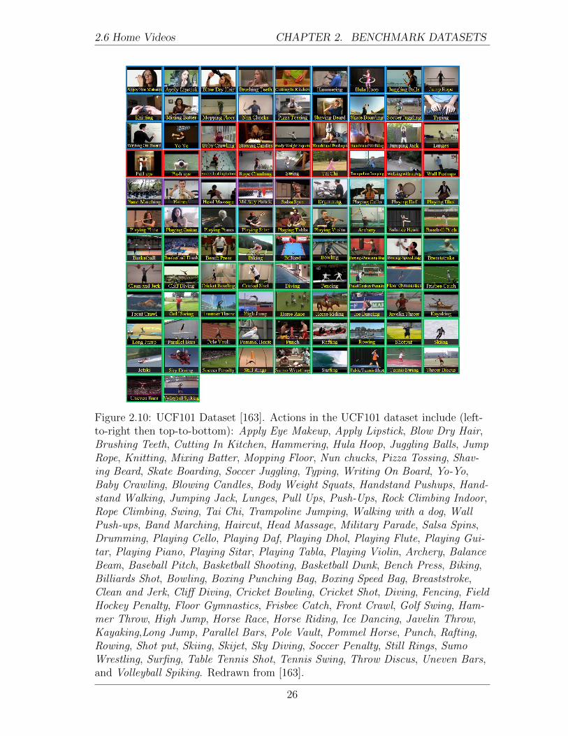
Figure 2.10: UCF101 Dataset [163]. Actions in the UCF101 dataset include (left-to-right then top-to-bottom): Apply Eye Makeup, Apply Lipstick, Blow Dry Hair,Brushing Teeth, Cutting In Kitchen, Hammering, Hula Hoop, Juggling Balls, JumpRope, Knitting, Mixing Batter, Mopping Floor, Nun chucks, Pizza Tossing, Shav-ing Beard, Skate Boarding, Soccer Juggling, Typing, Writing On Board, Yo-Yo,Baby Crawling, Blowing Candles, Body Weight Squats, Handstand Pushups, Hand-stand Walking, Jumping Jack, Lunges, Pull Ups, Push-Ups, Rock Climbing Indoor,Rope Climbing, Swing, Tai Chi, Trampoline Jumping, Walking with a dog, WallPush-ups, Band Marching, Haircut, Head Massage, Military Parade, Salsa Spins,Drumming, Playing Cello, Playing Daf, Playing Dhol, Playing Flute, Playing Gui-tar, Playing Piano, Playing Sitar, Playing Tabla, Playing Violin, Archery, BalanceBeam, Baseball Pitch, Basketball Shooting, Basketball Dunk, Bench Press, Biking,Billiards Shot, Bowling, Boxing Punching Bag, Boxing Speed Bag, Breaststroke,Clean and Jerk, Cliff Diving, Cricket Bowling, Cricket Shot, Diving, Fencing, FieldHockey Penalty, Floor Gymnastics, Frisbee Catch, Front Crawl, Golf Swing, Ham-mer Throw, High Jump, Horse Race, Horse Riding, Ice Dancing, Javelin Throw,Kayaking,Long Jump, Parallel Bars, Pole Vault, Pommel Horse, Punch, Rafting,Rowing, Shot put, Skiing, Skijet, Sky Diving, Soccer Penalty, Still Rings, SumoWrestling, Surfing, Table Tennis Shot, Tennis Swing, Throw Discus, Uneven Bars,and Volleyball Spiking. Redrawn from [163].
26

2.6 Home Videos CHAPTER 2. BENCHMARK DATASETS
Category Actions
1 Human-Object Interaction Apply eye makeup, apply lipstick, blowdry hair, brushing teeth, cutting inkitchen, hammering, hula hoop, jugglingballs, jump rope, knitting, mixing batter,mopping floor, nun chucks, pizza tossing,shaving beard, skate boarding, soccerjuggling, typing, writing on board, andyo-yo
2 Body-Motion Only baby crawling, blowing candles, bodyweight squats, handstand push-ups,handstand walking, jumping jack, lunges,pull ups, push ups, rock climbing indoor,rope climbing, swing, tight, trampolinejumping, walking with a dog, and wallpush-ups
3 Human-Human Interaction band marching, haircut, head massage,military parade, and salsa spin
4 Playing musical instruments drumming, playing cello, playing dad,playing dhol, playing flute, playing gui-tar, playing piano, playing sitar, playingtabla, and playing violin
5 Sports Archery, balance beam, baseball pitch,basketball, basketball dunk, benchpress, biking, billiard, bowling, boxing-punching bag, boxing-speed bag, breast-stroke, clean and jerk, cliff diving, cricketbowling, cricket shot, diving, fencing,field hockey penalty, floor gymnastics,frisbee catch, front crawl, golf swing,hammer throw, high jump, horse race,horse riding, ice dancing, javelin throw,kayaking, long jump, parallel bars, polevault, pommel horse, punch, rafting,rowing, shot-put, skiing, jets, sky div-ing, soccer penalty, still rings, sumowrestling, surfing, table tennis shot, ten-nis swing, throw discus, uneven bars,and volleyball spiking
Table 2.3: UCF101 Dataset categorization [163].
27

2.7 The Human Motion Databases CHAPTER 2. BENCHMARK DATASETS
tains 27, 801 videos belonging to 203 action classes, where each video can containmore than one activity. The set is randomly divided into 50% training, 25% vali-dation, and 25% test sets. The temporal action detection set contains 849 hours ofvideo, where the detection algorithm should identify the start and end frames of allactions present in the untrimmed test video sequence. Like trimmed and untrimmedrecognition sets, the set is randomly divided into 50% training, 25% validation, and25% test sets. mAP (2.2) is used to measure the performance of all three tasks.A detection is considered a true positive if the IoU score (2.3) between a predictedtemporal segment and the ground truth segment is greater than some constant κ.Authors report results on varying values of κ from 0.1 to 0.5 in increments of 0.1.
2.6.3 Discussion
The UCF101 dataset was one of the most challenging and largest datasets in actionrecognition and detection. Recently, the ActivityNet Dataset has taken the role andhas become one of the most difficult for its large-scale and unconstrained charac-teristic of the videos. Both UCF101 and ActivityNet datasets contain videos thatclosely resemble videos that can be found in the real-world. Thus, algorithms thatperform well in these datasets have great potential for use in real-life scenarios.
2.7 The Human Motion Databases
In efforts to collect videos that would capture the complexity of videos found inmovies and videos online, the large Human Motion Database (HMDB51 ) [83] wascreated by collecting videos from various sources, such as movies, YouTube, andGoogle videos.
2.7.1 HMDB51
A total of 51 actions were selected for the HMDB51 database, where the actionswere broadly categorized into five groups: 1) general facial actions, 2) facial actionswith object manipulation, 3) general body movements, 4) body movements withobject interaction, and 5) body movements for human interaction (see Table 2.5and Figure 2.11). There are a total of 6, 766 clips in the HMDB51 dataset with eachaction containing at least 102 clips. To test the strengths and weaknesses in contextof various nuisance factors, each video is annotated with a meta tag, which pro-vides information like camera viewpoint, presence/absence of camera motion, videoquality, number of actors involved in the action, and visible body part (see Table2.6). Three distinct training and testing splits are suggested for experimentation,where each split was generated to ensure that the clips from the same video did notappear in both the training and testing sets while there was an even distribution ofmeta tags across the sets. Each split contains 70 training and 30 testing videos withthe excess videos excluded from the split. All the videos in the dataset have beennormalized for a consistent height of 240 pixels and the widths have been scaled
28

2.7TheHuman
Motion
Datab
asesCHAPTER
2.BENCHMARK
DATASETS
Category Sub-categories Actions
1 Eating and Drinking Eating and Drinking drinking coffee, drinking beer
Food and Drink Preparation preparing pasta, preparing salad, making a sandwich, mixing drinks
Kitchen and Food Clean-up washing dishes
2 Sports, Exercise,and Recreation
doing aerobics zumba, step-aerobics
Martial arts kickboxing, karate, tai chi
Playing sports high jump, cricket, discus throw, javelin throw, paintball, long jump, bungeejumping, triple jump, shot put, dodgeball, hammer throw, skateboarding, mo-tocross, campfire, archery, volleyball, kickball, pole vault,field hockey, basketballlayup
Weightlifting clean and jerk, snatch
Gymnastics pommel horse, balance beam, tumbling, parallel bars, uneven bars
Cardiovascular equipment spinning
Racket sports table tennis, tennis serve, squash, lacrosse, racquetball, badminton
Equestrian sports polo, horseback riding
Climbing, spelunking, caving rock climbing
Water sports springboard diving, sailing, platform diving, windsurfing, water polo, kayaking
3 Socializing, Relax-ing, and Leisure
Dancing tango, cheerleading, cumbia, breakdancing, belly dancing
Musical Instrument playing bagpipes, harmonica, saxophone, guitar, flute, piano, violin, accordion
Arts and Entertainment ballet
29

2.7TheHuman
Motion
Datab
asesCHAPTER
2.BENCHMARK
DATASETS
Tobacco and Drug Use smoking hookah, smoking a cigarette
Playing Games hopscotch
4 Personal Care Washing, Dressing, andGrooming Oneself
putting on makeup, washing face, brushing hair, brushing teeth, doing nails, wash-ing hands, shaving, shaving legs, removing curlers
Washing, Dressing, andGrooming
getting a tattoo, piercing, and a haircut
5 Household Activities Household Management wrapping presents
Animals and Pets bathing dogs, grooming horse, walking the dog
Interior Maintenance, Re-pair, and Decoration
chopping wood, painting
Housework cleaning windows, vacuuming floor, polishing furniture, cleaning shoes, polishingshoes, ironing clothes, handwashing clothes
Vehicles fixing bicycle
Exterior Maintenance, Re-pair, and Decoration
shovelling snow
Lawn, Garden, and House-plants
lawn mowing
Table 2.4: ActivityNet Categorization [51].
30

2.7 The Human Motion Databases CHAPTER 2. BENCHMARK DATASETS
accordingly, ranging between 176 and 592 pixels, to maintain the original aspectratio. All videos are trimmed to contain one of 51 actions, and the location of eachaction is not provided as a ground truth. Thus, this dataset is useful for testingclassification.
Category Actions
1 General facial actions smile, laugh, chew, talk
2 Facial actions with objectmanipulation
smoke, eat, drink
3 General body movements cartwheel, clap hands, climb, climbstairs, dive, fall on the floor, backhandflip, hand-stand, jump, pull up, push up,run, sit down, sit up, somersault, standup, turn, walk, wave
4 Body movements with ob-ject interaction
brush hair, catch, draw sword, dribble,golf, hit something, kick ball, pick, pour,push something, ride bike, ride horse,shoot ball, shoot bow, shoot gun, swingbaseball bat, sword exercise, throw
5 Body movements for humaninteraction
fencing, hug, kick someone, kiss, punch,shake hands, sword fight
Table 2.5: HMDB51 Dataset categorization [83].
Property Labels
1 Visible Body Parts head, upper body, full body, lower body
2 Camera Motion motion, static
3 Camera Viewpoint front, back, left, right
4 Number of People involvedin the Action
single, two, three
5 Video Quality good, medium, ok
Table 2.6: HMDB51 Dataset Meta Tag Labels [83].
31

2.7 The Human Motion Databases CHAPTER 2. BENCHMARK DATASETS
Figure 2.11: HMDB51. Actions in the HMDB51 dataset include (left-to-right):brush hair, cartwheel, catch, chew, clap, climb, climb stairs, dive, draw sword, dribble,drink, eat, fall floor, fencing, flic flac, golf, hand stand, hit, hug, jump, kick, kick ball,kiss, laugh, pick, pour, pull-up, punch, push, push up, ride bike, ride horse, run, shakehands, shoot ball, shoot bow, shoot gun, sit, sit-up, smile, smoke, somersault, stand,swing baseball, sword exercise, sword, talk, throw, turn, walk, and wave. Redrawnfrom [83].
32
2.8 Challenges CHAPTER 2. BENCHMARK DATASETS
2.7.2 J-HMDB
To better understand and analyze the limitations and identify components of al-gorithms for improvement on overall accuracy on the HMDB51 dataset, a joint-annotated HMDB (J-HMDB) dataset has been made available [66]. Among the 51different human action categories that were collected for the HMDB51 dataset, cat-egories that mainly contain facial expressions (e.g. smiling), interaction with others(e.g. shaking hands), and very specific actions (e.g. cartwheels) were excluded. Asa result, 21 classes that involve a single individual performing the action has beenchosen, which includes: brush hair, catch, clap, climb stairs, golf, jump, kick ball,pick, pour, pull-up, push, run, shoot ball, shoot bow, shoot gun, sit, stand, swingbaseball, throw, walk, and wave.
There are 36 to 55 clips per action class with each clip containing about 15-40frames, summing to a total of 928 clips in the dataset. Each clip is trimmed suchthat the first and last frames correspond to the beginning and end of an action. Allclips have a spatial resolution of 320× 240 with a frame rate of 30 fps. The datasetis randomly split into three distinct sets for evaluation with the condition that theclips from the same video file are not used for both training and testing. For eachaction category, 70% of the videos are used for training, and 30% for testing witha relatively even distribution of the meta tags (e.g. camera position, video quality,motion, etc.). A 2D puppet model for annotation, which represents the human bodywith a set of 10 body parts connected by 13 joints (shoulders, elbows, wrists, hips,knees, ankles, and neck) and 2 landmarks (the face and the core) are provided toallow researchers to test their algorithms on both the spatiotemporal localizationand recognition of the specified actions.
2.8 Action Recognition and Detection Challenges
In efforts to encourage researchers in the vision community to develop action recog-nition and detection algorithms that can be effectively and efficiently applied innatural settings, an international workshop called the THUMOS Challenge tookplace annually from 2013 to 2015 and ActivityNet Challenge in 2016 in conjunctionwith various major conferences in computer vision [70, 71, 48, 161]. Three THUMOSchallenges: THUMOS’ 13, THUMOS’ 14, THUMOS’ 15, along with the ActivityNetchallenge will be surveyed in this section.
2.8.1 THUMOS’ 13
The very first THUMOS challenge, THUMOS’ 13, which took place in conjunctionwith the International Conference on Computer Vision (ICCV) in 2013, consisted oftwo tasks: the recognition task and the detection task. Both the recognition and thedetection tasks were based on videos from the UCF101 dataset (see section 2.6.1).Three training and testing splits were randomly generated such that for each split,18 of the 25 groups were used as training, and the rest as test data for each action.
33

2.8 Challenges CHAPTER 2. BENCHMARK DATASETS
Each participating team had to submit results to all three training and testing splitsthat were provided to qualify for the competition. For evaluation, various low-levelfeatures (e.g. STIP [87], SIFT [98], and DT [186] features (see section 3.1.2)) withlocation information, action attributes for the action classes (see Table 2.7), andbounding box annotations (for the detection task) were provided.
The objective of the recognition task was to predict which action amongst the101 action classes were present in each test clip. Each team was allowed to sub-mit multiple runs. 17 teams took part in the challenge, and a total of 30 runswere submitted. In this competition, 12 teams made use of low-level features (e.g.(improved) DT feature [186, 188], triangulation of SURF [119], 3D HOG [78] andHOF [88], and LPM [153]) (see section 3.1.2), and the rest used newly developedmid-level features (e.g. acton [230], online matrix factorization [19]). The most com-monly used methods of encoding and pooling were bag-of-words [159] and/or FVs[62] with a few using spatial/region pooling (see section 3.2). The top 10 performingalgorithms used VLAD [65] and/or FV encoding method along with (improved) DTfeatures and an SVM classifier. All teams used either the non-linear or linear SVMfor classification with one using neural networks (see section 4.2.2). Even thoughaction attribute information were provided for all videos, there were no submissionsthat made use of the class-level attributes to recognize the test data. The baselinerecognition result reported on the UCF101 data by November of 2012 was 43.9%[163], and the winner of the THUMOS 2013 challenge achieved an overall accuracyof 87.46% using VLAD+FV-encoded iDT features with a linear SVM [189], whichis a significant improvement within a year.
The goal of the detection task was to localize the bounding boxes provided inthe test videos and to identify the 24 pre-defined action classes. 10 of the 24 classeswere selected from the UCF11 dataset, which include: basketball shooting, cycling,diving, golf swing, tennis swing, trampoline jumping, volleyball spiking, and walk-ing the dog; and 14 additional classes: basketball dunk, cliff diving, cricket bowling,fencing, floor gymnastics, horseback riding, ice dancing, long jump, pole vault, ropeclimbing, salsa spin, skateboarding, skiing, ski-jet, soccer juggling, and surfing; wereadded to the challenge. A detected result was considered correct if the action classwas classified correctly and the intersection-over-union (2.3) was greater than orequal to 0.2. Unfortunately, no team took part in the localization task of the THU-MOS’ 13 challenge. It is worth noting here that although no team took part in thedetection task of the THUMOS’ 13 challenge, there were algorithms that reporteddetection results on other datasets, such as the UCF Sports dataset and the MSRAction Dataset II [173].
2.8.2 THUMOS’ 14
The second THUMOS challenge, THUMOS’ 14, took place the following year in con-junction with the 2014 European Conference on Computer Vision (ECCV). Similarto the previous THUMOS challenge, there were two main tasks in the THUMOS’
34

2.8Challen
gesCHAPTER
2.BENCHMARK
DATASETS
Class Attributes
Body Motion flipping, walking, running, riding, up down, pulling, lifting, pushing, diving, jumping up, jumping forward,jumping over obstacle, spinning, climbing up, horizontal, vertical up, vertical down, bending
Body Parts Visible head close-up, face close-up, upper body, lower body, full body, one hand, two hands
Number of People one, two, many
Object ball-like, big ball-like, stick-like, rope-like, sharp, circular, cylindrical, musical instrument, portal musicalinstrument, animal, boat-like
Outdoor grass, water, ocean/lake, court, sky, street/road, track, general
Indoor pool, office, court, gym, home, track, general
Posture sitting, sitting in front of a table-like object, standing, lying, handstand
Body Parts Used head, hands, arms, legs, foot
Body Part Articulation
Arm one arm motion, two arms motion, synchronized arm motion, alternate arm motion, one arm raised overhead, two arms raised over head, one arm raised chest level, two arms raised chest level, one arm open tothe side, two arms open to the side, one arm down, two arms down, one arm bent, two arms bent, one armstretched, two arms stretched, one arm swinging, two arms swinging
Leg synchronized leg motion, alternate leg motion, fold-unfold motion, up-down motion, up-forward motion,side-stretch motion, one leg raise, two legs raise, legs open to the side, one leg bent, two legs bent, one legstretched, two legs stretched
Hand throw-release motion, synchronized hand motion, one hand closed, two hands closed, one hand grab, twohands grab, one hand open, two hands open
Head facing down, facing up, facing front, facing sideways, straight position, tilted position
Torso down-forward motion, twist motion, bent position, straight up position
Feet touching ground, in air
Table 2.7: The 115 class-level attributes assigned to the 101 actions for the THUMOS’ 13 Challenge [70].
35
2.8 Challenges CHAPTER 2. BENCHMARK DATASETS
14 challenge: the recognition task and the temporal action detection task. The goalof the recognition task remained the same as the previous year, which was to pre-dict the presence/absence of an action class in a given sequence. The objectiveof the temporal action detection task, however, was to identify when which of thepre-defined 20 actions had occurred in the test clip without providing the spatiallocation. For both tasks, four types of data were provided: training, validation,background, and test. The training data were videos extracted from the UCF101dataset, which were temporally trimmed such that each sequence contained oneinstance of the action and all irrelevant frames were removed. The other threeparts (validation, background, and test data), on the other hand, were collections ofuntrimmed videos. As in the THUMOS’ 13 challenge, pre-computed low-level fea-ture of the iDT features along with the spatiotemporal information were providedfor all (training, validation, background, and test) datasets. Each team was grantedat most five submissions of the results for each task, where the run with the bestperformance was used to rank across other results.
For the action recognition task, the entire UCF101 dataset of temporally trimmedvideos was provided for training. The validation set contained 10 untrimmed videosfor each class tallying 1, 000 videos in total to allow participants to fine-tune theiralgorithms and to use as further training data, if necessary. Each validation videocontained a primary action with some containing one or more instances of otheraction classes. The background data, which contained 2, 500 clips, were videos rele-vant to each action, but did not contain an instance of any of the 101 action classes.For example, a clip of a basketball court without a basketball game taking placewas provided as background data for “basketball dunk”. Background data providedverification of the absence of action classes. The test data consisted of 1, 574 tem-porally untrimmed test videos, which contained one or multiple instances of one,multiple, or none of the action classes were provided as test data. 11 teams tookpart in the challenge and 35 runs were submitted. 10 participants used DT featureswhile 4 used CNNs. In addition, 9 teams used FVs in conjunction with iDT fea-tures (see section 3.1.2 and section 3.2.2). Beyond low-level features, participantsused various mid-level features such as face, body and eye features, audio, saliencyfeatures, and shot boundary detection. 10 teams used SVM for classification andone team used extreme learning [57, 181]. Using (2.1) and (2.2), the winner of theTHUMOS’ 14 action recognition challenge achieved an mAP score of 0.71 by usingiDT features with CNN and SVM as a classifier. The THUMOS’ 14 recognitiontask was deemed more challenging than the previous year’s as the test videos weretemporally untrimmed, which meant that significant portion of some videos did notcontain any of the 101 actions. Furthermore, variations of instances, where multipleor no instance of any actions were possibilities in test videos, was another factorthat made the classification task more challenging than the previous year’s. Theseadded features in the test videos were embedded to the competition to guide thenext generation of action recognition algorithms to be more useful in practical set-tings.
36

2.8 Challenges CHAPTER 2. BENCHMARK DATASETS
From the task of spatial and temporal detection, the THUMOS’ 14 detectionchallenge had been mitigated to temporal detection. The task mitigation led tocomputational complexity and annotation alleviation. Instead of 24 action classesas in the previous year’s challenge, the detection task called for localization of 20action classes (baseball pitch, basketball dunk, billiards, clean and jerk, cliff diving,cricket bowling, cricket shot, diving, frisbee catch, golf swing, hammer throw, highjump, javelin throw, long jump, pole vault, shot put, soccer penalty, tennis swing,throw discus, and volleyball spike). Similar to the recognition task, four datasets(training, validation, background, and test) were provided. The training data con-tained temporally trimmed videos from the UCF101 dataset of the 20 action classes,200 validation videos with temporal annotations (start and end time) of all instancesof the 20 actions were provided in the validation set, the same set of backgrounddata as in the recognition task were provided for the 20 actions, and 1, 574 tem-porally untrimmed videos were provided as test data. As in the recognition task,interpolated AP and mAP metrics were used to measure performance of each actionclass and each run, respectively. A detection was considered correct if the IoU score(2.3) was greater than 0.5 for the predicted time range and ground truth time range.3 teams took part in the challenge with 11 submissions in total. All three teams uti-lized the FV-encoded iDT with CNN features and used 1-vs-rest SVM over temporalwindows. The variation amongst the three approaches depended on using either theearly or late fusion of the features, system parameters (e.g. window size, step size,hard negatives), post-processing (re-scoring, thresholding), and/or combining withclassification scores. The top performing approach, which attained a score of 0.14was distinguished in the following three ways [128]. First, combining the window’sdetection score with video’s classification score for the same action class. Second,using additional features such as SIFT, colour moments, CNN, and MFCC. Third,using ASR in their classification process.
2.8.3 THUMOS’ 15
The third annual THUMOS challenge, THUMOS’ 15, took place in conjunctionwith the 2015 Conference on Computer Vision and Pattern Recognition (CVPR).Identical to previous years’ THUMOS challenges, the THUMOS’ 15 challenge alsocomprised of two tasks: the recognition task and the detection task. The objectivesof the recognition and detection tasks remained the same as the THUMOS’ 14 tasks,to detect the presence/absence of an action in a given clip and to temporally localizeand identify actions in a test video, respectively. Four datasets (training, validating,background, and testing) were provided, as before. The same temporally trimmed13, 320 videos from the UCF101 dataset were provided for the recognition task andselect videos for the chosen 20 actions of the localization task were provided in thetraining set. 2, 140 and 200 temporally untrimmed validation videos were providedfor the classification and detection tasks, respectively, the same 2, 980 backgroundvideos were provided for both tasks, and 5, 613 temporally untrimmed videos wereprovided for test in both tasks.
37

2.8 Challenges CHAPTER 2. BENCHMARK DATASETS
The same evaluation metrics, AP (2.1) and mAP (2.2), as in the THUMOS’14 challenge, were employed to evaluate the results on each action class and toevaluate the performance of a single run, respectively. The intersection-over-uniondefined overlap as in the previous challenges (2.3) was used, where the detection wasconsidered correct if the overlap was greater than 0.5. A total of 11 teams partici-pated in the recognition challenge and 52 runs were submitted. 10 of 11 teams usediDT features and ranked in the top 10 of the competition. Various other methodswere employed such as deep networks, MFCC, and multi-granularity analysis (VGG,C3D, iDT, and MFCC). Use of enhanced iDT, multi-granularity analysis (VGG),CNN (LCD), along with MFCC and ASR features and a combination of SVM anda logistic regression fusion classifier allowed the winner of the recognition challengeto attain an mAP score of 0.7384 [207]. Only one team took part in the tempo-ral action detection challenge for which they utilized FV-encoded iDTs, performedmulti-granular analysis using VGG and FV, embedded the shot boundary detectionmethod, and used an SVM classifier to attain an mAP score of 0.1830. With suchlow participation in the localization task, it is plausible that the datasets for the taskhad been too computationally demanding and not enough time had been grantedfor submission.
2.8.4 ActivityNet Challenge
In conjunction with CVPR 2016, the ActivityNet Large Scale Activity RecognitionChallenge took place. Similar to the THUMOS challenges, the ActivityNet Chal-lenge also comprised of two tasks: the classification task and the detection task.The objective of the classification challenge was to identify the label of the activ-ities that were present in a given long untrimmed video. The detection challengerequired an additional challenge of identifying the temporal extents of the activitiesthat were present in the given video. Similar to the THUMOS challenges, pre-computed features were provided (e.g. ImageNetShuffle and MBH global features,C3D frame-based features, and agnostic temporal activity proposals).
To evaluate the performance of each algorithm, mAP (equation (2.2)) and top-kclassification accuracy metrics were used. The top-k metric, which measures theprobability of the correct class attaining the top k confidence score for k ∈ Z+,provides additional information about the algorithm, but was not used to determinethe winner of the challenge. A detection was considered correct if the IoU score (2.3)was greater than 0.5. Only one submission was permitted per participant. A totalof 24 participants took part in the classification challenge and 6 in the temporal de-tection challenge. Algorithms that achieved top 10 performance in the classificationchallenge either used handcrafted iDT features, deep-learned convolutional features,or its combination to achieve an mAP score greater than 82.5. The winner of theuntrimmed video classification challenge achieved an mAP score of 93.2 by analyz-ing two complementary components of a video: visual and auditory information.The visual system takes an altered two-stream approach adopting the ResNet andInception V3 architectures, which are aggregated via top-k pooling and attention
38

2.9 Summary CHAPTER 2. BENCHMARK DATASETS
weighted pooling. The audio system, on the other hand, combines the FV-encodedstandard MFCC features trained on SVMs with audio-based CNNs. Many algo-rithms in the detection task temporally localized actions by either utilizing (i) thesliding temporal window approach or (ii) using LSTM-RNNs. The winner of theaction detection challenge achieved an mAP score of 42.5 using VLAD-encoded IDTcombined with C3D features on SVM classifiers.
2.8.5 Final Remarks on the Challenges
In this section, four action recognition and detection challenges that took place inconjunction with major conferences were examined. A quantitative summary of theTHUMOS’ 13, 14, 15, as well as the ActivityNet challenges are provided in Table 2.8.In the upcoming challenge, it is projected that the task of action proposal, whosegoal is to retrieve temporal (or spatiotemporal) regions that are likely to containactions, will be added. Furthermore, the classification task will be based on a largerdataset containing approximately 1, 000 action classes with more than 500 samplesper class and the detection task may be extended to the spatiotemporal domain.
2.9 Summary
In this chapter, numerous benchmark datasets have been introduced. Table 2.9summarizes the key features of the commonly used datasets.
Although significant progress has been made in collecting data to test variousaction recognition algorithms, current major datasets are deemed too unrealisticand/or disorderly. The availability of a systematic dataset that consists of natural-istic videos is crucial since the next plausible step in action recognition and detectionwould be to implement the next generation of algorithms into the real-world. Thus,in constructing the next benchmark dataset, a set of useful actions that make fre-quent appearance in security, robotics, entertainment, and health care should beconsidered. Furthermore, the parameters should vary in a systematic way to allowresearchers to quickly examine the effect caused by changes in illumination, viewingdirection, scale, clutter, recording setting, and performance nuance.
39
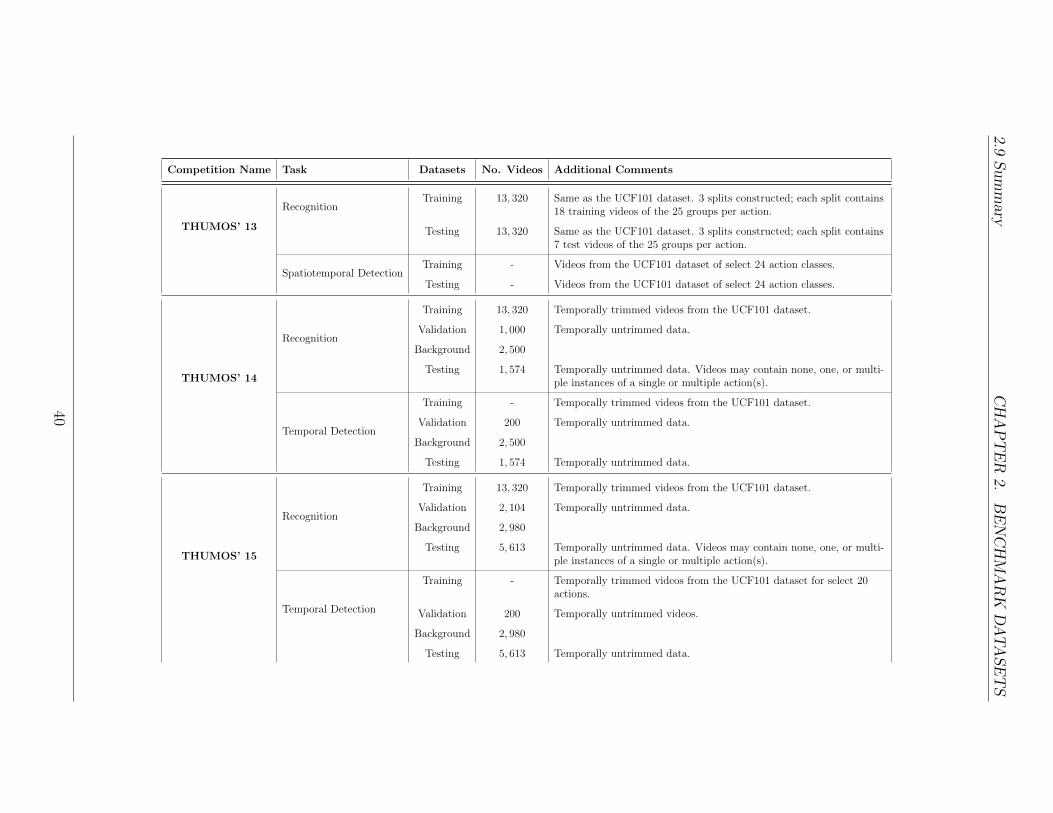
2.9Summary
CHAPTER
2.BENCHMARK
DATASETS
Competition Name Task Datasets No. Videos Additional Comments
THUMOS’ 13
RecognitionTraining 13, 320 Same as the UCF101 dataset. 3 splits constructed; each split contains
18 training videos of the 25 groups per action.
Testing 13, 320 Same as the UCF101 dataset. 3 splits constructed; each split contains7 test videos of the 25 groups per action.
Spatiotemporal DetectionTraining - Videos from the UCF101 dataset of select 24 action classes.
Testing - Videos from the UCF101 dataset of select 24 action classes.
THUMOS’ 14
Recognition
Training 13, 320 Temporally trimmed videos from the UCF101 dataset.
Validation 1, 000 Temporally untrimmed data.
Background 2, 500
Testing 1, 574 Temporally untrimmed data. Videos may contain none, one, or multi-ple instances of a single or multiple action(s).
Temporal Detection
Training - Temporally trimmed videos from the UCF101 dataset.
Validation 200 Temporally untrimmed data.
Background 2, 500
Testing 1, 574 Temporally untrimmed data.
THUMOS’ 15
Recognition
Training 13, 320 Temporally trimmed videos from the UCF101 dataset.
Validation 2, 104 Temporally untrimmed data.
Background 2, 980
Testing 5, 613 Temporally untrimmed data. Videos may contain none, one, or multi-ple instances of a single or multiple action(s).
Temporal Detection
Training - Temporally trimmed videos from the UCF101 dataset for select 20actions.
Validation 200 Temporally untrimmed videos.
Background 2, 980
Testing 5, 613 Temporally untrimmed data.
40
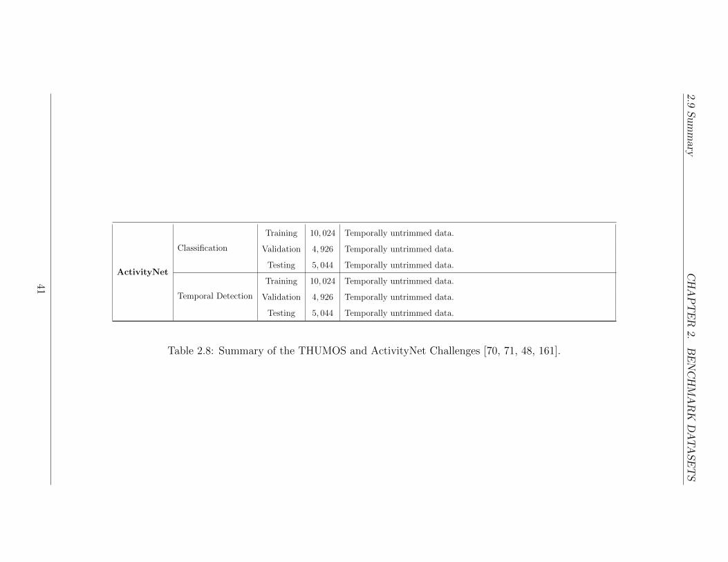
2.9Summary
CHAPTER
2.BENCHMARK
DATASETS
ActivityNet
Classification
Training 10, 024 Temporally untrimmed data.
Validation 4, 926 Temporally untrimmed data.
Testing 5, 044 Temporally untrimmed data.
Temporal Detection
Training 10, 024 Temporally untrimmed data.
Validation 4, 926 Temporally untrimmed data.
Testing 5, 044 Temporally untrimmed data.
Table 2.8: Summary of the THUMOS and ActivityNet Challenges [70, 71, 48, 161].
41

2.9Summary
CHAPTER
2.BENCHMARK
DATASETS
Dataset Year No. Actions No. Actors No. Videos Frame Rate (fps) Cam. View Cam. Motion Bckg clutter Task
KTH [148] 2004 6 25 600 25 Frontal/Side No No Recognition, Temporal Detection*
Weizmann [14] 2005 10 9 600 25 Frontal/Side No No Recognition, Spatiotemporal Detection*
MPII Cooking Activities [141] 2012 65 12 44 29.4 Frontal/Side No No Recognition, Temporal Detection
MPII Cooking 2 [142] 2015 67 30 273 29.4 Frontal/Side No No Recognition, Temporal Detection
CMU Crowded Videos [76] 2007 5 65 training
25-30 Frontal/Side No Yes Recognition, Spatiotemporal Detection48 test
MSR Action I [219] 2009 3 10 16 15 Frontal/Side No Yes Spatiotemporal Detection
MSR Action II [20] 2010 3 10+ 54 14-15 Frontal/Side No Yes Spatiotemporal Detection
CMU Sports (Ballet) [34] 16 6 Frontal/Side No No
CMU Sports (Tennis) [34] 2003 6 2 N/A N/A Side No No -
CMU Sports (Soccer) [34] 8 R Multiple Yes Yes
UCF Sports [140, 162] 2008 10 R 150 10 Multiple Yes Yes Spatiotemporal Detection
Olympic Sports [121] 2010 16 R 783 N/A Multiple Yes Yes Recognition
Sports-1M [73] 2014 487 R 1, 133, 158 - Multiple Yes Yes Recognition
Hollywood1 [88] 2008 8 R 475 23-25 Multiple Yes Yes Recognition
Hollywood2 [107] 2009 10 + 6 scenes R 2, 517 23-29 Multiple Yes Yes Recognition
UCF11 (YouTube) [96] 2009 11 R 1, 600 29 Multiple Yes Yes Spatiotemporal Detection
UCF50 [139] 2012 50 R 6, 681† 25 or 29 Multiple Yes Yes Spatiotemporal Detection
UCF101 [163] 2012 101 R 13, 320 25 or 29 Multiple Yes Yes Spatiotemporal Detection
ActivityNet [51] 2015 203 R 19, 994 mostly 30 Multiple Yes Yes Recognition, Temporal Detection
HMDB51 [83] 2011 51 R 6, 766 30 Multiple Yes Yes Recognition
J-HMDB [66] 2013 21 R 928 30 Multiple Yes Yes Recognition, Spatiotemporal Detection
Table 2.9: Summary of Benchmark Datasets. R indicates that the datasets were extracted from realistic videos. Thus, thenumber of actors cannot be determined. (*) Although the intended use of these datasets is to recognize actions, the authorsprovide ground truths (e.g. start and end frames, silhouettes) allowing the evaluation of temporal/spatiotemporal detectionpossible. (†) The official report of the UCF50 dataset [139] documents a total of 6676 videos in the UCF50 dataset. However,the downloadable UCF50 dataset contains 6681 videos.
42
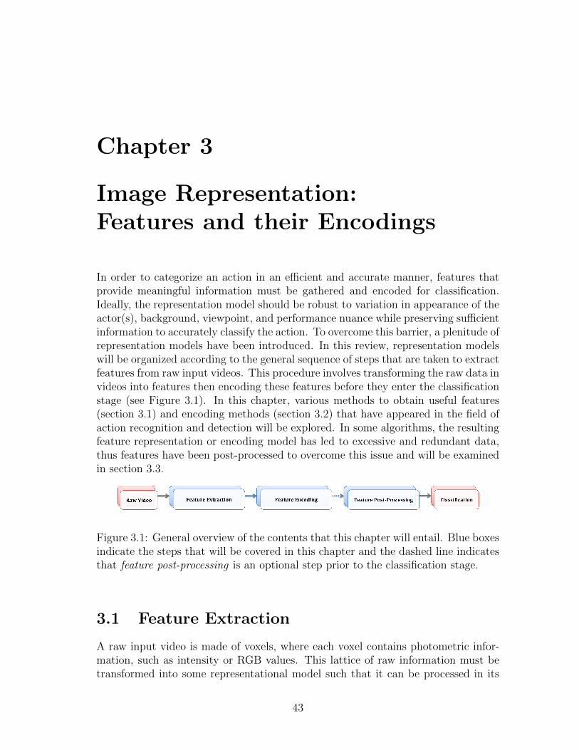
Chapter 3
Image Representation:Features and their Encodings
In order to categorize an action in an efficient and accurate manner, features thatprovide meaningful information must be gathered and encoded for classification.Ideally, the representation model should be robust to variation in appearance of theactor(s), background, viewpoint, and performance nuance while preserving sufficientinformation to accurately classify the action. To overcome this barrier, a plenitude ofrepresentation models have been introduced. In this review, representation modelswill be organized according to the general sequence of steps that are taken to extractfeatures from raw input videos. This procedure involves transforming the raw data invideos into features then encoding these features before they enter the classificationstage (see Figure 3.1). In this chapter, various methods to obtain useful features(section 3.1) and encoding methods (section 3.2) that have appeared in the field ofaction recognition and detection will be explored. In some algorithms, the resultingfeature representation or encoding model has led to excessive and redundant data,thus features have been post-processed to overcome this issue and will be examinedin section 3.3.
Figure 3.1: General overview of the contents that this chapter will entail. Blue boxesindicate the steps that will be covered in this chapter and the dashed line indicatesthat feature post-processing is an optional step prior to the classification stage.
3.1 Feature Extraction
A raw input video is made of voxels, where each voxel contains photometric infor-mation, such as intensity or RGB values. This lattice of raw information must betransformed into some representational model such that it can be processed in its
43
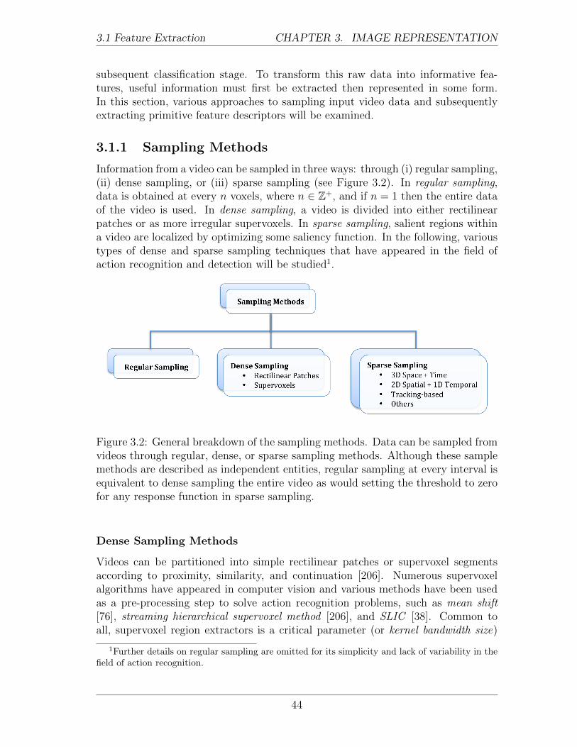
3.1 Feature Extraction CHAPTER 3. IMAGE REPRESENTATION
subsequent classification stage. To transform this raw data into informative fea-tures, useful information must first be extracted then represented in some form.In this section, various approaches to sampling input video data and subsequentlyextracting primitive feature descriptors will be examined.
3.1.1 Sampling Methods
Information from a video can be sampled in three ways: through (i) regular sampling,(ii) dense sampling, or (iii) sparse sampling (see Figure 3.2). In regular sampling,data is obtained at every n voxels, where n ∈ Z+, and if n = 1 then the entire dataof the video is used. In dense sampling, a video is divided into either rectilinearpatches or as more irregular supervoxels. In sparse sampling, salient regions withina video are localized by optimizing some saliency function. In the following, varioustypes of dense and sparse sampling techniques that have appeared in the field ofaction recognition and detection will be studied1.
Figure 3.2: General breakdown of the sampling methods. Data can be sampled fromvideos through regular, dense, or sparse sampling methods. Although these samplemethods are described as independent entities, regular sampling at every interval isequivalent to dense sampling the entire video as would setting the threshold to zerofor any response function in sparse sampling.
Dense Sampling Methods
Videos can be partitioned into simple rectilinear patches or supervoxel segmentsaccording to proximity, similarity, and continuation [206]. Numerous supervoxelalgorithms have appeared in computer vision and various methods have been usedas a pre-processing step to solve action recognition problems, such as mean shift[76], streaming hierarchical supervoxel method [206], and SLIC [38]. Common toall, supervoxel region extractors is a critical parameter (or kernel bandwidth size)
1Further details on regular sampling are omitted for its simplicity and lack of variability in thefield of action recognition.
44
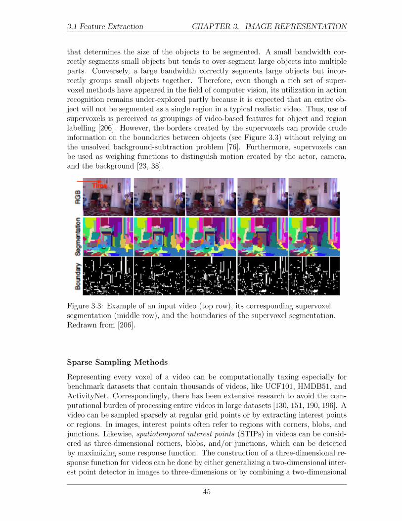
3.1 Feature Extraction CHAPTER 3. IMAGE REPRESENTATION
that determines the size of the objects to be segmented. A small bandwidth cor-rectly segments small objects but tends to over-segment large objects into multipleparts. Conversely, a large bandwidth correctly segments large objects but incor-rectly groups small objects together. Therefore, even though a rich set of super-voxel methods have appeared in the field of computer vision, its utilization in actionrecognition remains under-explored partly because it is expected that an entire ob-ject will not be segmented as a single region in a typical realistic video. Thus, use ofsupervoxels is perceived as groupings of video-based features for object and regionlabelling [206]. However, the borders created by the supervoxels can provide crudeinformation on the boundaries between objects (see Figure 3.3) without relying onthe unsolved background-subtraction problem [76]. Furthermore, supervoxels canbe used as weighing functions to distinguish motion created by the actor, camera,and the background [23, 38].
Figure 3.3: Example of an input video (top row), its corresponding supervoxelsegmentation (middle row), and the boundaries of the supervoxel segmentation.Redrawn from [206].
Sparse Sampling Methods
Representing every voxel of a video can be computationally taxing especially forbenchmark datasets that contain thousands of videos, like UCF101, HMDB51, andActivityNet. Correspondingly, there has been extensive research to avoid the com-putational burden of processing entire videos in large datasets [130, 151, 190, 196]. Avideo can be sampled sparsely at regular grid points or by extracting interest pointsor regions. In images, interest points often refer to regions with corners, blobs, andjunctions. Likewise, spatiotemporal interest points (STIPs) in videos can be consid-ered as three-dimensional corners, blobs, and/or junctions, which can be detectedby maximizing some response function. The construction of a three-dimensional re-sponse function for videos can be done by either generalizing a two-dimensional inter-est point detector in images to three-dimensions or by combining a two-dimensional
45
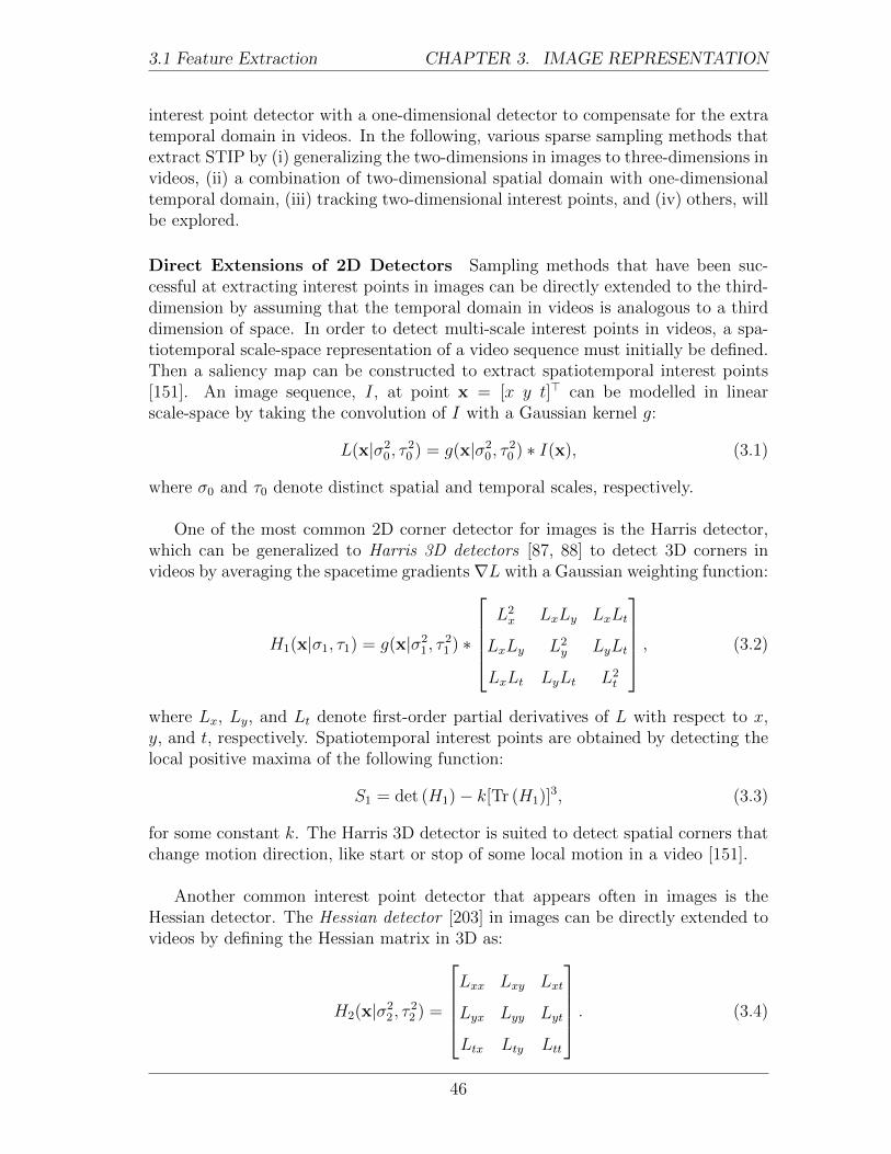
3.1 Feature Extraction CHAPTER 3. IMAGE REPRESENTATION
interest point detector with a one-dimensional detector to compensate for the extratemporal domain in videos. In the following, various sparse sampling methods thatextract STIP by (i) generalizing the two-dimensions in images to three-dimensions invideos, (ii) a combination of two-dimensional spatial domain with one-dimensionaltemporal domain, (iii) tracking two-dimensional interest points, and (iv) others, willbe explored.
Direct Extensions of 2D Detectors Sampling methods that have been suc-cessful at extracting interest points in images can be directly extended to the third-dimension by assuming that the temporal domain in videos is analogous to a thirddimension of space. In order to detect multi-scale interest points in videos, a spa-tiotemporal scale-space representation of a video sequence must initially be defined.Then a saliency map can be constructed to extract spatiotemporal interest points[151]. An image sequence, I, at point x = [x y t]> can be modelled in linearscale-space by taking the convolution of I with a Gaussian kernel g:
L(x|σ20, τ
20 ) = g(x|σ2
0, τ20 ) ∗ I(x), (3.1)
where σ0 and τ0 denote distinct spatial and temporal scales, respectively.
One of the most common 2D corner detector for images is the Harris detector,which can be generalized to Harris 3D detectors [87, 88] to detect 3D corners invideos by averaging the spacetime gradients ∇L with a Gaussian weighting function:
H1(x|σ1, τ1) = g(x|σ21, τ
21 ) ∗
L2x LxLy LxLt
LxLy L2y LyLt
LxLt LyLt L2t
, (3.2)
where Lx, Ly, and Lt denote first-order partial derivatives of L with respect to x,y, and t, respectively. Spatiotemporal interest points are obtained by detecting thelocal positive maxima of the following function:
S1 = det (H1)− k[Tr (H1)]3, (3.3)
for some constant k. The Harris 3D detector is suited to detect spatial corners thatchange motion direction, like start or stop of some local motion in a video [151].
Another common interest point detector that appears often in images is theHessian detector. The Hessian detector [203] in images can be directly extended tovideos by defining the Hessian matrix in 3D as:
H2(x|σ22, τ
22 ) =
Lxx Lxy Lxt
Lyx Lyy Lyt
Ltx Lty Ltt
. (3.4)
46

3.1 Feature Extraction CHAPTER 3. IMAGE REPRESENTATION
Regions with a local maxima of the determinant of the 3D Hessian (i.e. S2 =|detH2|) for some particular position and scale correspond to a centre of a blob ina video [151].
2D (Spatial) Detector with a 1D (Temporal) Detector Beyond varying thescale-space support in space and time separately via constants σ and τ , the temporaldimension can be managed by generating an even more distinct filter in the temporaldomain. The temporal domain can be treated differently from the spatial domain byapplying distinct filters for each domain [29, 122]. The cuboid detector [29] couplesa Gaussian filter in the spatial domain and a Gabor filter in the temporal domainto create a response function that is applicable in the spatiotemporal domain. Fora given video I(x), the response function is defined as:
R(x) = [I(x) ∗ g(x, y|σ) ∗ heven(t|τ, ω)]2 + [I(x) ∗ g(x, y|σ) ∗ hodd(t, τ, ω)]2, (3.5)
where g(x, y|σ) is the 2D Gassian smoothing kernel applied along the spatial dimen-sions (x, y), and heven(t|τ, ω) = − cos (2πtω)e−t
2/τ2 and hodd(t|τ, ω) = − sin (2πtω)e−t2/τ2
are quadrature pair of 1D Gabor filters applied along the temporal domain t. σ andτ correspond to spatial and temporal scales of the detector, respectively, and ω thecentre frequency2. It can be observed that the cuboid detector is best matched toan intensity pattern that oscillates sinusoidally along the temporal dimension andsmoothed in the spatial dimension with a low-pass (Gaussian) filter. Conversely, thesmallest response would be generated in regions that lack temporally distinguishingfeatures. Hence, it is well suited to detect temporally varying patterns even whileproviding little response to those that remain static. In comparison to the aforemen-tioned detectors, 3D Harris and Hessian, the cuboid detector extracts a denser set offeatures and is consequently computationally more expensive to follow-on processing[190].
Tracking-based Detectors Determining good features to track is an alternativeapproach to obtaining a useful set of sample points. Since points found in struc-tureless regions are impossible to track, it would be helpful to remove them fromthe sampling set. The decision to retain or remove a point can be made using thegood-features to track criterion [154], which is determined by the eigenvalues of theauto-correlation matrix, a matrix intimately related to 2D Harris. This samplingtechnique is incorporated in the (improved) dense trajectory features [186, 188],which has shown to be very effective as it is one of the strongest contemporaryfeatures in application to action recognition.
Other Sparse Sampling Methods There are many other sparse sampling meth-ods that were not mentioned in detail, such as the Harris-Laplace [111], Hessian-Laplace [112], Difference of Gaussian (DoG) [98] and maximally stable extremal
2The centre frequency for the Gabor function refers to the frequency in which the filter yieldsthe greatest response. ω can be set to 4/τ to reduce the number of parameters involved in equation(3.5) [29, 122].
47

3.1 Feature Extraction CHAPTER 3. IMAGE REPRESENTATION
region (MSER) [109] detectors. The Harris-Laplace, which uses the Harris andLaplacian functions to find and select points, respectively, is capable of detectingcorners and other junctions, pairs and triplets of edge segments to represent contoursinvariant of scale and rotation changes [114]. The Hessian-Laplace localizes pointsin space and scale by taking the local maxima of the determinant of a Hessian andthe Laplacian-of-Gaussian, respectively [113]. Since the shape of the Hessian kernelfits better to blob-like structures than corners, the Hessian-Laplace detector is usedto extract various types of blobs [114]. The DoG detector, which is often used inaccordance with a 3D histogram of gradient location and orientation and togetherreferred to as SIFT, uses the difference of images of different scales convolved with aGaussian function to identify the locations of edges and blob-like structures. MSERextracts blobs by expanding regions according to their intensity levels by graduallyincreasing some threshold value. The value that enforces the smallest rate of changeis selected as the threshold to extract MSER and has shown to provide useful de-tection results [94, 114, 177].
The extracted features can be pruned using spatial, temporal, or motion statis-tical measures [96]. Excessive amount of features can be judged by comparing thenumber of features extracted in a single frame to the average amount of featurespresent per frame. Spatial outliers can be spotted using neighbourhood information.Lastly, PageRank [115, 129] can be used to identify consistency of the extracted fea-ture to others to classify them as inliers.
Discussion on Sampling Methods
Regular, dense, and sparse sampling methods have been described as independententities in this section, but we must bear in mind that these methods are not dis-joint. That is, regularly sampling at every interval would be equivalent to densesampling the entire video, which is equivalent to setting the threshold to 0 for anyresponse function in sparse sampling.
Videos that largely consist of static backgrounds that pose no useful informationto recognize actions (e.g. videos in the KTH dataset) benefit from sparse sampling asfeatures obtained through dense sampling provide no useful data [190]. Furthermore,extracting features sparsely across videos provide data compactness leading to com-putational efficiency. When coupled with appropriate descriptors and classifiers (tobe described in more detail in the following section and chapter, respectively), thesedetectors extract sufficient data to acceptably differentiate between human actions.However, it was observed that sparse sampling methods fall behind the accuracy inrecognition that dense (or regular) sampling methods are able to provide, especiallyin videos with contextual information (e.g. UCF Sports, Hollywood2) [190]. Thisresult may be due to the fact that (i) the data extracted using these detectors tendto be too sparse and (ii) the contextual information, such as equipment or scene,can provide additional information to improve classification results. Furthermore,many saliency functions that are used to extract features assume that videos contain
48

3.1 Feature Extraction CHAPTER 3. IMAGE REPRESENTATION
several instances of motion or appearance that are significantly different in eitherdirection of motion or the boundary between the background and the actor. Thisassumption leads to failure in capturing smooth motions (as in Figure 3.4a) andgenerates spurious detects along object boundaries (see Figure 3.4b) [75].
The sparse motion detectors mentioned in this paper (e.g. cuboid detector, KLTtracker, DT) can be used in motion compensated or non-compensated videos. Thesedetectors are expected to fire at the presence of motion whether it be camera motionor motion created by different body parts of an actor. Often in action recognition, itis understood that motion created by the object’s body provides useful information.Thus, the output results of these detectors must be used with caution as they mayrespond to some dominant motion due to camera movement or an actor occupying alarge portion of the field of view, which may or may not be the desired informationthat one wishes to obtain for their recognition algorithm.
The choice of data extraction can affect the computational efficiency but canalso influence the accuracy of the recognition step as sampling is the first step in therecognition procedure. Thus, the data extraction technique must be chosen withcaution as it can heavily influence or deter the outcome of the results in followingprocessing steps.
3.1.2 Feature Descriptors
Once a sampling method has been selected, information that would characterizethe structure of the region must be represented in some useful way as a descriptorbefore it enters the classification stage. In the following, the feature descriptors havebeen split into general primitive and specialized primitive features as illustrated inFigure 3.5. General primitive features refer to features that can be obtained directlyfrom raw input videos, which then can be used directly in the classification module.Specialized primitive features refer to features that are extracted from raw inputvideos and require additional processing into auxiliary features before they enterthe classification stage. In this section, some common primitive feature descriptorsas well as its associated auxiliary feature descriptors that have appeared in the actionrecognition and detection literature will be studied.
General Primitive Features
General primitive features refer to features that can be directly extracted from rawvideos after some sampling method has been chosen (regular, dense, or sparse) andare transformed in a way such that it can be processed directly by some chosenclassification method. General primitive features can be divided into four broadcategories: filter-, flow-, convolutional neural network (CNN)-based, and others.Here, each of these categories will be examined.
49

3.1 Feature Extraction CHAPTER 3. IMAGE REPRESENTATION
(a) Blue arrow indicates the direction of motion. Two motions are illustrated in thisexample: circular motion (left) and the figure ‘8’ motion (right). The 3D plots ofmotion through time are illustrated (bottom) with blue ellipsoids showing detectedinterest points. All detected interest points were non-informative, and were onlydetected due to the boundaries that formed as the arm moved with the edge of theframe.
(b) Spacetime interest points detected on regions affected by varying lightingconditions. STIP detectors are sensitive to lighting conditions, therefore aredetected in regions with bright light or shadows.
Figure 3.4: Examples of commonly occurring motions that fail to produce usefulinterest points. Redrawn from [75].
50

3.1 Feature Extraction CHAPTER 3. IMAGE REPRESENTATION
Figure 3.5: General breakdown of feature descriptors. Features can be obtained fromraw videos by describing them using general primitive features or specialized prim-itive features. While general primitive features can be used to train and test dataimmediately, specialized primitive features must be further processed into auxiliaryfeatures before the features enter the classification stage.
Filter-based Descriptors Filter-based approaches can be categorized into twotypes: (i) gradient-based and (ii) oriented bandpass filter-based descriptors. Gradient-based methods rely on the assumption that the local appearance and shapes of anobject can be portrayed by their local intensity gradient or edge directions. Orientedbandpass filter-based approaches use oriented filters to decompose videos into basiccomponents using local orientation and scale. Notably, gradient-based approachesare an example of (high-pass) oriented filters, which have received a particularlylarge research focus. Hence, they are dealt separately from the more general ori-ented bandpass filters in the following.
A rich set of gradient-based descriptors have appeared in the field of action recog-nition. Some descriptors that have made frequent appearance in the field include:histogram of oriented gradients (HOG) [25, 191], HOG3D [78], cuboid descriptor[29], scale-invariant feature transform (SIFT) [98], gradient location-orientation his-togram (GLOH) [113], local trinary patterns (LTP) [211], and spatiotemporal (ST)patches [152]. HOGs store spatially oriented gradient to capture appearance infor-mation of the action. HOG3D extends HOG descriptors by storing spatiotemporaloriented gradients to store shape and motion information together. The cuboid de-scriptor [29] concatenates three gradient channels (Gx, Gy, Gt) into a single vectorto form a single feature vector for each neighbourhood. SIFT [98], which is coupledwith a scale-invariant region detector, DoG, uses 3D histograms to represent thegradient locations and orientations. The 2D SIFT descriptor uses polar coordinates
51

3.1 Feature Extraction CHAPTER 3. IMAGE REPRESENTATION
to obtain the gradient magnitudes and orientations, and the 3D SIFT descriptor[149] uses an additional angle to represent the direction of the gradient to incorpo-rate temporal information. The location and orientation bins in 2D/3D SIFT areweighed by the gradient magnitudes. Instead of quantizing the location informationon a Cartesian grid as in 2D/3D SIFT, GLOH quantizes them on a log-polar gridto increase robustness and distinctiveness [114]. LTPs compare intensities of theneighbouring pixels between preceding and succeeding frames to the current frameto determine the direction of motion [211, 79]. ST patches uses spatiotemporal gra-dients to estimate the motion of the sampled regions to obtain a rank of the STpatch. The constraint based on the rank provides information on motion withoutexplicitly computing the optical flow and spatial information (e.g. uniform intensity,edge-, and corner-like features) [152].
Although many of these oriented gradient-based descriptors provide computa-tional efficiency to gather crucial information, such as appearance and/or motion,they are very sensitive to illumination changes. Often, these descriptors do notprovide sufficient information and must be used in parallel with other descriptorsthat possess distinguishing characteristics (e.g. HOG is often found with HOF) toovercome its limitation.
Spatiotemporal oriented bandpass filters can decompose an image sequence intobasic components using the dimension of local orientation and scale (i.e. angularand radial frequencies). Consequently, various types of oriented filters have been ap-plied to a range of dynamic image understanding tasks, such as action recognitionand detection [123]. These representation models tend to be capable of character-izing image dynamics without explicitly requiring flow recovery nor segmentationof videos [24]. Two particular approaches of spatiotemporal oriented filtering havebeen commonly applied to actions: 3D Gabor filters [24, 123] and Gaussian deriva-tive filters [67]. Both 3D Gabor and Gaussian derivative filters are typically appliedin quadrature pairs and combined to produce some local energy measurement. Oftensubsequent processing is involved, such as normalization and/or combination of filteroutputs. The normalization process provides robustness to photometric variations[24], while combining filter outputs (e.g. appearance marginalization [28]) attemptto gather information on image dynamics that is invariant to spatial appearance.The filter outputs can also be combined to yield explicit motion estimates or othermeasurements of image motion [49].
Representations based on spatiotemporal oriented bandpass filters tend to berobust to illumination changes, in-class variations, and occlusion. Many researcherschoose to use Gaussian derivative filters for its separability and recursive componentsto keep the representation computationally efficient [24, 28]. However, some filterresponses (e.g. bandpass filters) pose sensitivity to irrelevant appearance attributes.Furthermore, these filters tend to be sensitive to scale changes, which is problematicsince the actor/action size is inconsistent between and within each video.
52

3.1 Feature Extraction CHAPTER 3. IMAGE REPRESENTATION
Optical Flow-based Descriptors Optical flow-based algorithms have appearedfrequently in various action recognition algorithms. Optical flow provides data thatcan be used in two ways: (i) to extract information on motion and (ii) for trackingpurposes. Here, some common optical flow-based representation models that haveappeared in the action recognition literature for each method will be explored.
Optical flow can be used to recognize actions by describing the motion of theactor. A standard optical flow algorithm can be applied to stabilized figure-centricvolumes to capture motion created by different parts of the body (see Figure 3.7b)[34, 94]. By separating the optical flow into horizontal and vertical components (asin Figure 3.7d) then blurring them (via Gaussian as in Figure 3.7e), an artificial setof motion channels are created [34, 36]. Often, the Kanade-Lucas-Tomasi (KLT)tracker is used to estimate local motion in a hierarchical manner to obtain the initialflow for the next level [177].
Histograms of Optical Flow (HOF) captures local motion of the pattern by quan-tizing the orientation of the optical flow vectors. While such characterization ofmotion is sufficient in distinguishing highly distinct actions (e.g. “walk” vs. “wave”in the KTH dataset), it fails to distinguish fine differences in actions (e.g. “box”vs. “clap” in the KTH dataset). Thus, simple description of motion combined withinformation on appearance (e.g. HOG) can yield more accurate recognition resultsas has been observed in more complicated datasets, such as the Hollywood1 dataset[88].
The Motion Boundary Histogram (MBH) is a descriptor that uses derivativesof optical flow for each horizontal and vertical directions, Ix and Iy, respectively[26, 186]. By computing the spatial derivatives for each flow field, the local gra-dient orientations and magnitudes can be found to construct a local orientationhistogram. Since MBH computes the gradient of optical flow, constant motion issuppressed and only the information regarding changes in the flow field are kept.Thus, MBH provides a simple way to suppress constant motion (e.g. camera motion)while preserving local relative motion of pixels (e.g. motion boundaries/foregroundmotion) (see Figure 3.8 right). This is an appealing feature, especially for recogniz-ing actions in realistic videos, since they tend to contain severe camera motion [186].Furthermore, the majority of the texture information from the static background iseliminated as the derivatives of the trajectories are considered.
With optical flow, physical properties of the flow pattern can be extracted viakinematic features, such as divergence, vorticity (or curl), symmetric and antisym-metric optical flow field, second and third principal invariants of flow gradient andrate of strain tensor [3, 63]. Kinematic features are perceived as independent forcesthat act on the object and capture information regarding motion only. For exam-ple, divergence captures information on the amount of axial motion, expansion, andscaling effects. Vorticity (or curl), on the other hand, highlights the circular mo-tion created by the human body or part of the human body. Thus, motions of the
53

3.1 Feature Extraction CHAPTER 3. IMAGE REPRESENTATION
hand toward the camera would be well captured by divergence; in contrast, rotarymotions of the hand parallel to the image plane would be well characterized by acurl. The kinematic features collectively provide a unique spatiotemporal patterndescription of the human action.
Dense trajectory (DT) features [186] were introduced as another form of descrip-tors that track the path of sampled motion (see Figure 3.6b), which have madefrequent appearance in the field of action recognition and detection [186, 228]. DTfeatures first require dense sampling of feature points at each frame, which arepruned using good-features to track. Then each of the sampled points are trackedusing optical flow to obtain its trajectory. The trajectory descriptor is obtainedby concatenating the normalized displacement vectors. These features are oftencombined with other features (e.g. HOG, HOF, MBH) aggregated along the trajec-tories. Various dense trajectory models that would enhance the original DT model[186] have been proposed [69, 188]. One approach was to cluster the dense tra-jectories to detect the dominant direction of motion and consider relative motionbetween the trajectories to gather object-background and object-object information[69]. Another approach was to explicitly estimate camera motion [188] by matchingfeature points between frames using SURF descriptors [9] and dense optical flow[154]. This particular camera motion compensated trajectory feature is referred toas the improved dense trajectory (iDT) feature and has appeared frequently in actionrecognition and detection literature [11].
(a) KLT Trajectories
(b) Dense Trajectories
Figure 3.6: Examples of KLT and dense trajectories of the “kiss” action from theHollywood2 dataset. Redrawn from [188].
Optical flow has been successful in various applications (e.g. tracking). In fact,some approaches have benefited from using optical flow-based algorithms to trackhumans, body parts, and interest points yielding good action recognition results(see under Specialized Primitive Features - Tracking-based Models). However, theability to estimate motion accurately and consistently has numerous challenges as-sociated, such as motion discontinuities (e.g. occlusion), aperture problems, andlarge illumination variations (e.g. appearance changes).
54

3.1 Feature Extraction CHAPTER 3. IMAGE REPRESENTATION
(a) Original Frame. (b) Optical Flow ~F =[Fx Fy
]>.
(c) The opticalflow vector ~F issplit into hori-zontal (Fx (top))and vertical(Fy (bottom))components.
(d) Horizontal and vertical op-tical flows are half-wave recti-fied to produce F+
x (top left),F−x (top right), F+
y (bottomleft), and F−y (bottom right).
(e) Half-wave rectified motionsare blurred into Fb+x (top left),Fb−x (top right), Fb+y (bottomleft), and Fb−y (bottom right).
Figure 3.7: The actor can be tracked to obtain a stabilized figure-centric volume. Astandard optical flow algorithm applied on a stabilized volume captures the motioncreated by the local regions in the volume. Redrawn from [34].
55
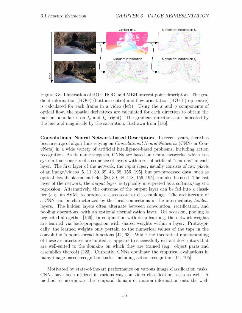
3.1 Feature Extraction CHAPTER 3. IMAGE REPRESENTATION
Figure 3.8: Illustration of HOF, HOG, and MBH interest point descriptors. The gra-dient information (HOG) (bottom-centre) and flow orientation (HOF) (top-centre)is calculated for each frame in a video (left). Using the x and y components ofoptical flow, the spatial derivatives are calculated for each direction to obtain themotion boundaries on Ix and Iy (right). The gradient directions are indicated bythe hue and magnitude by the saturation. Redrawn from [186].
Convolutional Neural Network-based Descriptors In recent years, there hasbeen a surge of algorithms relying on Convolutional Neural Networks (CNNs or Con-vNets) in a wide variety of artificial intelligence-based problems, including actionrecognition. As its name suggests, CNNs are based on neural networks, which is asystem that consists of a sequence of layers with a set of artificial “neurons” in eachlayer. The first layer of the network, the input layer, usually consists of raw pixelsof an image/videos [5, 11, 30, 39, 43, 68, 156, 195], but pre-processed data, such asoptical flow displacement fields [30, 39, 68, 118, 156, 195], can also be used. The lastlayer of the network, the output layer, is typically interpreted as a softmax/logisticregression. Alternatively, the outcome of the output layer can be fed into a classi-fier (e.g. an SVM) to produce a class score or class rankings. The architecture ofa CNN can be characterized by the local connections in the intermediate, hidden,layers. The hidden layers often alternate between convolution, rectification, andpooling operations, with an optional normalization layer. On occasion, pooling isneglected altogether [166]. In conjunction with deep-learning, the network weightsare learned via back-propagation with shared weights within a layer. Prototypi-cally, the learned weights only pertain to the numerical values of the taps in theconvolution’s point-spread functions [44, 93]. While the theoretical understandingof these architectures are limited, it appears to successfully extract descriptors thatare well-suited to the domains on which they are trained (e.g. object parts andassemblies thereof) [223]. Currently, CNNs dominate the empirical evaluations inmany image-based recognition tasks, including action recognition [11, 195].
Motivated by state-of-the-art performance on various image classification tasks,CNNs have been utilized in various ways on video classification tasks as well. Amethod to incorporate the temporal domain or motion information onto the well-
56
3.1 Feature Extraction CHAPTER 3. IMAGE REPRESENTATION
established 2D CNN architecture has been the main branching point of many algo-rithms in video classification. The most intuitive approach would be to replace 2Dconvolution and/or pooling operations with 3D ones to account for the additional(temporal) domain in videos [5, 68, 73, 155, 175]. Alternatively, the temporal infor-mation in videos can be summarized into a single RGB image such that standard 2DCNNs can be applied to recognize actions [11]. Recurrent neural networks (RNN),which are capable of learning temporal dynamics by explicitly considering the se-quences of CNN activations in a recurring manner, is another approach taken toaccount temporal dimension in videos [5, 30, 104, 118, 157]. To account for RNN’sinability to learn long-range temporal relationships, numerous algorithms suggestembedding long short-term memory (LSTM) units into the architecture to allow thenetwork to learn to recognize and synthesize temporal dynamics [5, 30, 104, 118].Recent methods resort to CNNs to obtain feature vectors of images [59, 104, 105, 212]or iFV-encoded iDT features with HOG, HOF, and MBH feature descriptors [220] asinputs to LSTM-RNN. Processing images in a per frame basis keeps track of whichfeatures are occurring when, allowing temporal detection of actions to be possible[212].
Another route that has been explored is the two-stream model [156], inspiredby biology [47], which decouples the appearance and motion components of a video[41, 157, 231]. The appearance stream takes framewise spatial input (e.g. RGBvalues) while the motion stream takes motion input (e.g. optical flow values [30, 41,68, 118, 156, 195, 231], motion vectors [224]). The two streams can be fused at thefinal stage of their respective architectures [30, 41, 68, 118, 156, 195], or sooner viaconvolutional fusion to put the channel responses in two streams that occur at thesame pixel location into correspondence [41]. Alternatively, the two streams can befused via introduction of residual connections between the paths [40]. In the stan-dard two-stream approach, computing the optical flow is expensive and the mosttimely step. Thus, rather than employ the most sophisticated dense optical flowtechniques, some have relied on cruder block-based matching approaches, as em-ployed for compression, which the authors refer to as “motion vectors” [224]. Theseapproaches, however, exhibit coarser structure than optical flow and may containnoise and inaccurate movements.
One CNN-based algorithm takes a completely different approach by redefining“action” as a change that it brings to the environment (see Figure 3.9). Thus,features before the action (at the pre-conditioned state) and after the action (at theeffect state) are aggregated using a Siamese network to represent an action [195].
The specificity of the features increases at higher layers of the network [166, 223].Thus, reducing the number of layers and neurons in each layer could depreciate theoverall performance of the system [73, 223]. Although the state-of-the-art perfor-mance in complex datasets are achieved using CNNs with many layers, it is done ata high computational cost [73]. To compensate for computational complexity, oneapproach applies PCA-whitening between layers on a stacked ISA network [92]. Al-
57

3.1 Feature Extraction CHAPTER 3. IMAGE REPRESENTATION
Figure 3.9: One algorithm defines actions as transformations brought to the environ-ment (i.e. pre-conditioned state × action = effect). Two transformations, kick (toprow) and jump (bottom row), are illustrated with their respective pre-conditioned(left columns) and effect (right columns) states. Redrawn from [195].
ternatively, a network can be separated into two streams that processes each frameof a video with two different spatial resolutions: (i) downsampled frames at half theoriginal spatial resolution, and (ii) a smaller spatial window at the original resolu-tion (e.g. centre region if videos are obtained from video sharing services to takeadvantage of the camera bias shot by amateur recorders) [73]. Another obstaclethat hinders the use of CNN-based methods is the amount of training data thatis required to construct a reliable system [73, 156]. Two of the largest benchmarkdatasets available, UCF101 and HMDB51, are considered too small to train a CNN-based video classification program from scratch [156, 195]. Thus, Sports-1M [73],a dataset containing more than a million videos, is often used to train the system.Since datasets as large as Sports-1M are typically constructed with some degree ofautomaticity, it leads to corruption of data, accumulating even more challenges atthe training and testing stages. Alternatively, the networks can be pre-trained onlarge static image recognition datasets (e.g. ImageNet [27]). However, such pre-training may cause the final network to bias towards appearance information overmotion, an undesirable trait for action recognition and detection in videos.
Other General Primitive Feature Descriptors Not all descriptors that haveappeared in the action recognition literature can be categorized as either filter-, flow-,or CNN-based representation models. Here, a select few other general primitive fea-ture descriptors that do not fall under these categories that possess noteworthycharacteristics are mentioned. They are: eSURF [9], MACH filter [140], and TCCAfeatures [77].
The extended Speeded Up Robust Features (eSURF) is a descriptor based onHaar-wavelet responses (dx, dy, dt) along the three axes [203] based on SURF [9].The feature vector is constructed by summing the weighed responses of the Haar-wavelets as sampled uniformly across each interest point (
∑dx,∑dy,∑dt). The
Haar-wavelet responses are weighed with a Gaussian to account for geometric de-formations and localization errors [9].
58

3.1 Feature Extraction CHAPTER 3. IMAGE REPRESENTATION
The maximum average correlation height (MACH) filter [140] is one of few algo-rithms that considers condensing a collection of data into a single template. Intra-class variations of an action is generalized into a single template by optimizing fourperformance metrics: average correlation height (ACH), average correlation energy(ACE), average similarity measure (ASM), and output noise variance (ONV). It usesspatiotemporal regularity flow (SPREF) to obtain the direction that best representsthe overall regularity of the volume (i.e. the direction in which the pixel intensitieschange the least) instead of other motion estimators to avoid challenges that occurdue to motion discontinuities, aperture problems, and large illumination variations.The SPREF flow field volume of each example is converted using a Clifford FourierTransform (CFT) for its efficiency, which is used to synthesize the MACH filter.The composite template video is obtained by combining the mean of the CFTs, thenoise covariance matrix, the average power spectral density, and the average simi-larity matrix to minimize ACE, ASM, and ONV while maximizing the ACH.
Tensor canonical correlation analysis (TCCA) features [77] consider videos asthird-order tensors with three modes (or axes). Third-order tensors can share anysingle or multiple modes. Thus, if a canonical transformation, a transformationthat maximizes the correlation of two multi-dimensional arrays, is applied to themodes that are not shared, then two types of TCCA can be produced: the joint-shared mode and the single shared-mode. The joint-shared mode allows any twomodes (or axes) (i.e. a plane or section in the video) to be shared and applies thecanonical transformation to the remaining single mode. It is found that a singlepair of canonical directions would maximize the inner product of the output tensors(or canonical objects) for the joint-shared modes. The single-shared mode, on theother hand, allows any single mode (i.e. a scan line of a video) to be shared andapplies the transformation to the remaining two modes. Here, two pairs of freetransformations maximize the inner product of the canonical objects for the single-shared modes. A single pairing of joint-shared mode TCCA preserves discriminativeinformation, whereas the double pairing of single-shared mode TCCA preserves lessoriginal data resulting in more flexibility in its information. Thus, the joint-sharedmode TCCA is used to filter inter-class differences (e.g. difference between actions)while the single-shared mode TCCA features are permissive to intra-class variations(e.g. difference in appearance).
Specialized Primitive Features and Auxiliary Features
Some algorithms require extraction of primitive features and further refinement intoauxiliary features before they can be useful to a classifier, especially the methods thatwere proposed in the earlier years of action recognition. Some examples of special-ized primitive features include silhouettes/contours and object tracks. Silhouette-/contour- and tracking-based features and the corresponding auxiliary features aredescribed in the following.
59

3.1 Feature Extraction CHAPTER 3. IMAGE REPRESENTATION
Silhouette-/Contour-based Models Numerous cognitive studies have shownthat humans are capable of extracting various useful information from silhouettes,such as recognizing objects, labelling parts, and comparing similarities to othershapes [8, 10]. Thus, a video of silhouettes may provide sufficient information forrecognition even while being robust to lighting conditions and invariant to the ap-pearance of the person. Once the silhouettes of the actors are extracted, informationcan be described in various forms. Silhouettes can either be directly converted into1D signals, converted into binary or scalar images then described using moments,or they can be stacked to form space-time volumes. A sample of each type of auxil-iary silhouette features, which include R Transforms, motion energy images, motionhistory images, motion history volumes, and spacetime volumes, will be describedbelow as a sample of such approaches.
R transforms are shape descriptors that convert silhouette images to 1D signals.By taking the squared sum of the Radon transform, commonly used to detect linesin images, over varying radii, a translation invariant Radon transform is defined al-lowing video alignment to match the position of the actor unnecessary. Furthermore,to resolve the scale sensitivity problem of Radon transforms, R is normalized. Thisimproved extension of the Radon transform, the R transform, attracted attentionto earlier action recognition algorithms that were silhouette-based (see [164, 198]).
Binary images of silhouettes called motion energy images (MEI) can be con-structed by accumulating the difference between silhouettes in subsequent framesand a scale-valued image, referred to as motion history images (MHI) can be con-structed to store the recency of motion that occurred at every pixel (see Figure3.10a). MEIs and MHIs together provide information on the location and the tem-poral history of the motion, respectively. These images have been further describedusing Hu moments [55] to draw further comparisons with other actions [100]. Manysilhouette-based algorithms have shown sensitivity to object’s displacement and ori-entation to the camera. This problem can be resolved by replacing the silhouettemotion indicating function with a silhouette occupancy function to create motionhistory volumes (MHV) instead of MHIs (see Figure 3.10b) [201]. Although MHVshave this appealing feature of viewpoint invariance with the use of an occupancyfunction, it is a great challenge to obtain an accurate function that would preciselymodel x-, y-, z-coordinates of where the object of interest is especially in videosgathered in uncontrolled settings, such as the web.
A sequence of silhouettes or its contours/boundaries can be concatenated alongthe temporal axis to create an image feature that captures the relationship betweenspace and time of a person’s action called spacetime volumes (STV) (see Figure3.10c). Information on the location of the general body parts (e.g. head, torso, andextremities) can be obtained by calculating the average time it takes for every pointinside the STV to reach the contour via a random-walk process [14] or differentialgeometry [213]. The Poisson equation can be used to identify the motion saliencyof moving parts and their orientations [14]. While MHVs and STVs appear similar,
60

3.1 Feature Extraction CHAPTER 3. IMAGE REPRESENTATION
MHVs illustrate the recency function through its 3D reconstruction, while temporalinformation cannot be observed in STVs.
Although silhouettes/contours provide useful information, obtaining accuratesegmentation of an actor is not guaranteed, especially in situations where the back-ground is not static as background subtraction remains an unsolved problem incomputer vision. Furthermore, the view angle can alter a person’s silhouette dras-tically and the features inside the boundary cannot be delineated since a person isrepresented as a single region.
Tracking-based Models As briefly mentioned in the optical flow section, track-ing can be perceived as an extreme example of optical flow. Tracking algorithms canbe utilized in action recognition by (i) tracing the trajectory of the entire actor in avideo to segment the actor from the background (see Figure 3.11a) [17, 34, 59, 157]or (ii) by tracking body parts (see Figure 3.11b) [35, 50, 61, 135, 136, 208] or localinterest regions [35, 60].
Tracking-based methods are potentially robust to variations in appearance ofeach actor or local region and have been shown to yield impressive results on low-resolution videos [34]. Despite significant progress, however, tracking remains anunsolved problem in computer vision as initializing tracking can be difficult as canmaintaining tracks over an extended period of time, especially in scenes with clut-tered or dynamic backgrounds. Moreover, since feature trackers often assume con-stant appearance of image patches over time, this assumption can pose problemswhen the appearance of the object changes, especially when two objects merge (oc-clude) or split (deocclude) [87]. Furthermore, the output of a tracker tends to benoisy, susceptible to drifting and illumination changes, causing problems in its sub-sequent steps when representing the action.
Final Remarks on Feature Descriptors
In this section, a select number of popularly used feature descriptors for humanactions were examined. Once the type of sampling method has been determined,primitive features can be obtained from raw videos. These primitive features caneither be encoded directly or must be converted into auxiliary features before it isencoded to enter the classification stage. Historically, the field of action recogni-tion approached the task of action recognition using specialized primitive featuresas it contained useful information. However, features that rely on these special-ized primitive features were deemed unfavourable as background-subtraction andtracking remain unsolved problems in computer vision. A mixture of filter- andflow-based algorithms merged. Now, the state-of-the-art performance is achieved byCNN-based algorithms.
61

3.1 Feature Extraction CHAPTER 3. IMAGE REPRESENTATION
(a) Examples of MEI (left) and MHI (right) of the sitting motion. Redrawnfrom [16].
(b) Examples of Motion History Volumes. Motion history volumes of actions(left-to-right): sit-down, walk, kick, and punch are illustrated using the colourspectrum, where blue indicates oldest motion and red indicates the most recentmotion. Redrawn from [201].
(c) Examples of a spacetime volume (STV) for actors performing a jumpingjack, walk, and run actions. Redrawn from [14].
(d) The solution to the Poisson equation reveal the shape of an actor. Thevalues are encoded using the colour spectrum, where low values are encodedby blue and high values are encoded by red. Regions far from the core (theextremities and the head) have low values, therefore are encoded in blue.
Figure 3.10: Examples of various silhouette-based models in action recognition.
62
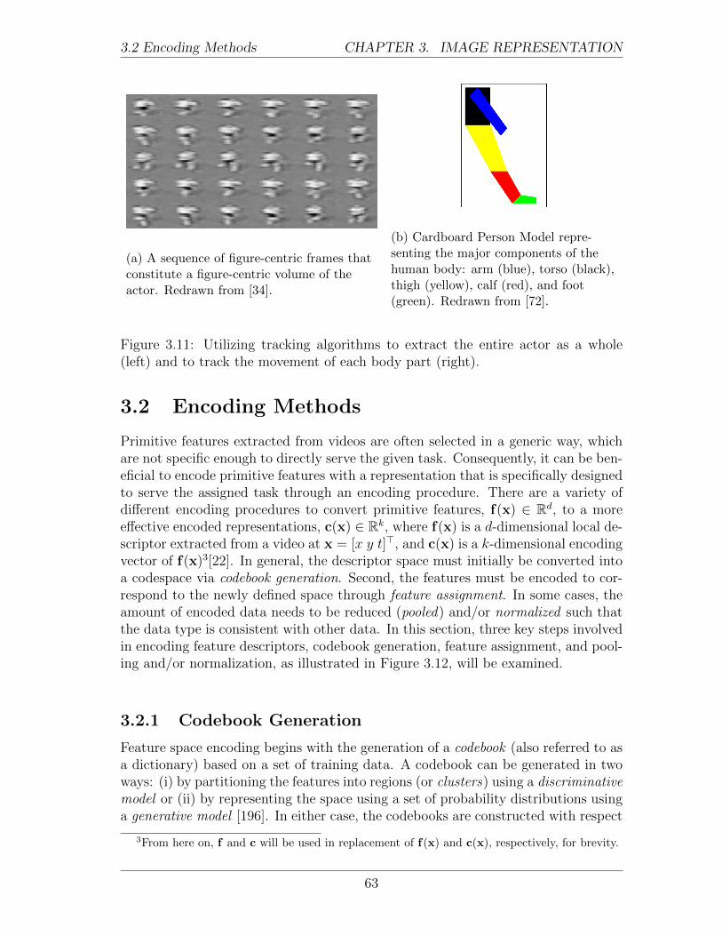
3.2 Encoding Methods CHAPTER 3. IMAGE REPRESENTATION
(a) A sequence of figure-centric frames thatconstitute a figure-centric volume of theactor. Redrawn from [34].
(b) Cardboard Person Model repre-senting the major components of thehuman body: arm (blue), torso (black),thigh (yellow), calf (red), and foot(green). Redrawn from [72].
Figure 3.11: Utilizing tracking algorithms to extract the entire actor as a whole(left) and to track the movement of each body part (right).
3.2 Encoding Methods
Primitive features extracted from videos are often selected in a generic way, whichare not specific enough to directly serve the given task. Consequently, it can be ben-eficial to encode primitive features with a representation that is specifically designedto serve the assigned task through an encoding procedure. There are a variety ofdifferent encoding procedures to convert primitive features, f(x) ∈ Rd, to a moreeffective encoded representations, c(x) ∈ Rk, where f(x) is a d-dimensional local de-scriptor extracted from a video at x = [x y t]>, and c(x) is a k-dimensional encodingvector of f(x)3[22]. In general, the descriptor space must initially be converted intoa codespace via codebook generation. Second, the features must be encoded to cor-respond to the newly defined space through feature assignment. In some cases, theamount of encoded data needs to be reduced (pooled) and/or normalized such thatthe data type is consistent with other data. In this section, three key steps involvedin encoding feature descriptors, codebook generation, feature assignment, and pool-ing and/or normalization, as illustrated in Figure 3.12, will be examined.
3.2.1 Codebook Generation
Feature space encoding begins with the generation of a codebook (also referred to asa dictionary) based on a set of training data. A codebook can be generated in twoways: (i) by partitioning the features into regions (or clusters) using a discriminativemodel or (ii) by representing the space using a set of probability distributions usinga generative model [196]. In either case, the codebooks are constructed with respect
3From here on, f and c will be used in replacement of f(x) and c(x), respectively, for brevity.
63
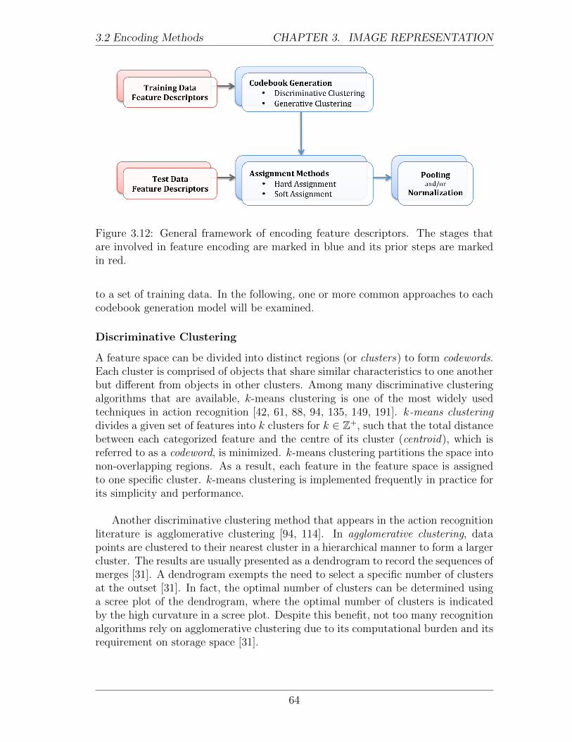
3.2 Encoding Methods CHAPTER 3. IMAGE REPRESENTATION
Figure 3.12: General framework of encoding feature descriptors. The stages thatare involved in feature encoding are marked in blue and its prior steps are markedin red.
to a set of training data. In the following, one or more common approaches to eachcodebook generation model will be examined.
Discriminative Clustering
A feature space can be divided into distinct regions (or clusters) to form codewords.Each cluster is comprised of objects that share similar characteristics to one anotherbut different from objects in other clusters. Among many discriminative clusteringalgorithms that are available, k-means clustering is one of the most widely usedtechniques in action recognition [42, 61, 88, 94, 135, 149, 191]. k-means clusteringdivides a given set of features into k clusters for k ∈ Z+, such that the total distancebetween each categorized feature and the centre of its cluster (centroid), which isreferred to as a codeword, is minimized. k-means clustering partitions the space intonon-overlapping regions. As a result, each feature in the feature space is assignedto one specific cluster. k-means clustering is implemented frequently in practice forits simplicity and performance.
Another discriminative clustering method that appears in the action recognitionliterature is agglomerative clustering [94, 114]. In agglomerative clustering, datapoints are clustered to their nearest cluster in a hierarchical manner to form a largercluster. The results are usually presented as a dendrogram to record the sequences ofmerges [31]. A dendrogram exempts the need to select a specific number of clustersat the outset [31]. In fact, the optimal number of clusters can be determined usinga scree plot of the dendrogram, where the optimal number of clusters is indicatedby the high curvature in a scree plot. Despite this benefit, not too many recognitionalgorithms rely on agglomerative clustering due to its computational burden and itsrequirement on storage space [31].
64

3.2 Encoding Methods CHAPTER 3. IMAGE REPRESENTATION
Generative Clustering
A feature space can be represented using probability distributions such as the Gaus-sian Mixture Model (GMM). Given a set of feature descriptors (from a trainingset), a weighted sum of Gaussian functions can be used to model the (training set)feature space. Typically, the parameters (i.e. the weight, mean vector and covari-ance matrix of individual Gaussian distribution) that would optimally represent thefeature space are trained through maximum-likelihood (ML) estimation using theexpectation-maximization (EM) algorithm. The learned parameters of the GMM(e.g. mean vectors and covariance matrices) provide information on the mean infor-mation of the codewords as well as the shape of their distributions [196]. While first-and second-order statistical information provides information that would assist inimproving the accuracy of the classification procedure, it is computationally expen-sive to obtain and store first- and second-order statistical information compared todiscriminative models and not as compact.
Discussion on Codebook Generation
The size of the codebook (i.e. number of clusters or GMMs) is a crucial parameterin codebook generation as it affects the computational cost and classification accu-racy. Up to a certain point, recognition performance has been empirically shown toimprove with the growth of the codebook size (i.e. number of clusters or GMMs).Exceptions to this general point can be observed as the performance plateaus whenthe size of the codebook exceeds some threshold [130]. Moreover, an excessivelylarge codebook size can harm the accuracy level due to over-fitting of the data orover-partition of the feature space. The thresholds to yield an optimal codebook isdependent on the dimension and sampling strategy of the feature descriptor [130].
Features with higher dimensions require more codewords to divide the featurespace. Thus, a larger codebook size would be necessary for optimal performance.Sparsely sampled feature points tend to be more scattered in the feature space thandensely sampled feature points. Thus, to avoid over-partitioning of the codebook(i.e. to ensure that every cluster is affiliated with a feature), the codebook sizeshould be smaller in data obtained via sparse sampling as opposed to data obtainedthrough dense sampling. Moreover, the distribution of densely sampled descriptorsin the feature space would not provide useful high-order statistics (e.g. variance),which would affect the type of information that should be obtained in the subsequentassignment step. Thus, although generative models provide more information, dis-criminative clustering would be the preferred choice with densely sampled featuresas they provide a more compact clustering leading to computational efficiency.
While the codebook size is a key parameter, the optimal codebook size is depen-dent on many factors. Unfortunately, there is no theoretical solution that would findthe optimal codebook size. Thus, readers should bear in mind that many algorithmsthat use k-means clustering or GMMs often report best results based on k that wasobtained through trial-and-error.
65

3.2 Encoding Methods CHAPTER 3. IMAGE REPRESENTATION
3.2.2 Assignment Methods
With a codebook generated using a set of features from the training set, a new set offeatures can be quantized according to the clusters (or codewords) in the pre-definedcodebook. Features can either be assigned to a single word through hard assignmentor into multiple words through soft assignment. Here, some examples of these twotypes of quantization assignment methods are examined.
Hard Assignment
Hard assignment methods assign feature descriptors from videos to a single codewordin the codebook. The most common hard assignment quantization method thatappears in action recognition algorithms is vector quantization (VQ), which assignsa feature descriptor to the nearest codeword in the codebook. Instead of assigninga binary value to the closest codeword as in VQ, a weight can be assigned to thenearest codeword to quantitatively indicate the similarity between the feature anda small subset of close codewords as in salient coding (SC) [58]. For its simplicityand efficiency, VQ is widely used in many action recognition algorithms [42, 61, 82,107, 135, 148, 209]. Since hard assignments represent each feature by the nearestcodeword, features that are nearly equidistant to multiple codewords are prone tochange even when small adjustments are made at the codebook generation stage.This ambiguity causes hard assignment-based methods to be unstable, which canaggravate recognition accuracy rates [196].
Soft Assignment
To overcome the ambiguity that hard assignment quantization techniques pose, fea-tures can be assigned to multiple codewords instead of one through soft assignment.Soft assignment methods can be further broken down into two categories: combina-torial and contrasting. Combinatorial methods express features as a combination ofthe codewords while constrasting methods describe features by alluding to the dif-ferences between features and codewords. Here, some common approaches of eachsoft assignment methods that have appeared in the action recognition literature areconsidered.
Combinatorial Features can be expressed as a combination of all or just a fewcodewords in the codebook. To naively encode a feature vector based on all code-words would yield an unreliable feature assignment to the codespace, especially thelinkages that are made with distant codewords [97]. Thus, a select number of code-words in the codebook should be considered. The weight to assign the degree ofmembership of feature, f , to codeword, ci, can be determined by solving the follow-ing optimization problem [130]:
arg minc‖f − Cc‖22 + λψ(c), (3.6)
66

3.2 Encoding Methods CHAPTER 3. IMAGE REPRESENTATION
where C = [c1 . . . ck] is a codebook with k codewords ci for i = 1, . . . , k, and λis a constant that controls the strength of the regularization term ψ(c). Some ex-amples of assignment methods that assign features, f , to codewords, c, using (3.6)include: orthogonal matching pursuit (OMP) [176], sparse coding (SpC) [210], localcoordinate coding (LCC) [217], and locality-constrained linear coding (LLC) [192],which differ by their regularization term, ψ. The regularization term enforces vary-ing properties of c.
The orthogonal matching pursuit (OMP) approximates c by considering thenumber of nonzero elements of c, the l0-norm of c. Unfortunately, l0-norms arenon-convex and to obtain a solution to (3.6) with ψ(c) = ‖c‖0 requires some heuris-tic strategy. Thus, to counter the non-convexity of the l0-norm, the regularizationterm in (3.6) can be replaced with an l1-norm (i.e. ψ(c) = ‖c‖1), which is referredto as sparse coding (SpC).
It was empirically observed that SpC is helpful when the codewords are local(i.e. when non-zero coefficients are assigned to codewords (or bases) near the featurevector (the data to be encoded)) [192, 217]. Since this locality is not guaranteed theway (3.6) is set up in SpC, the locality constraint of SpC can be explicitly enforcedby modifying the regularization term as ψ(c) = ‖e � |c|‖1, such that 1>c = 1 asin local coordinate coding (LCC)4. Unfortunately, SpC and LCC require solving anl1-optimization problem, which is computationally expensive and problematic forlarge-scale problems. As a result, a practical assignment scheme called the locality-constrained linear coding (LLC) [192] was designed as a fast-implementation of LCCby defining the regularization term as ψ(c) = ‖e � c‖22, such that 1>c = 1 fore = exp
(eσ
), where e ensures that similar patches have similar codes by assigning
weights proportional to how similar each codeword is to the feature vector.
Among various soft combinatorial assignments that were introduced in this sec-tion (see Table 3.1 for a summary), LLC is the most popularly used for its fastimplementation. Put simply, LLC assigns each feature as a linear combination ofm-nearest codewords in the codebook of size k for m � k ∈ Z+. As a point ofcomparison, note that VQ and LLC base their assignments on the 1-nearest and m-nearest codewords, respectively. However, the weighted sum of multiple codes allowLLCs to better capture the relationship between similar descriptors that share thesame codewords than the hard assignment quantization methods [192]. AlthoughLLC is faster than other combinatorial methods, the least square problem (3.6) thatneeds to be solved to find the m nearest words remains a computational burden ofthe LLC combinatorial assignment method.
Unlike the combinatorial assignment methods that were introduced earlier, thelocalized soft-assignment [97] does not involve solving the least-squares problem
4e in LCC and LLC denote dist(f , C) = [dist(f , c1) · · · dist(f , ck)]>, where dist(f , ci) is theEuclidean distance between f and ci for ci ∈ C.
67
3.2 Encoding Methods CHAPTER 3. IMAGE REPRESENTATION
(3.6), rather a normalized weight is assigned with respect to m-nearest codewordsfor m < k in a codebook of size k. Although it has a computational advantage overLLC, and is the most computationally efficient combinatorial assignment approach,with a comparable accuracy rate, a constant value that determines the softness ofthe assignment is present as a free parameter.
Assignment Type Regularization Term ψ(c)
Orthogonal Matching Pursuit (OMP) ‖c‖0Sparse Coding (SpC) ‖c‖1Local Coordinate Coding (LCC) ‖e� |c|‖1 such that 1>c = 1
Locality-Constrained Linear Coding (LLC) ‖e� |c|‖22, where e = exp(eσ
)Table 3.1: List of regularization terms for combinatorial soft assignment meth-ods. The coefficients that determines the degree of membership between fea-ture f and codeword ci is determined by solving the least-squares problem:arg minc ‖f − Cc‖22 + λψ(c) given a codebook C = [c1 · · · ck]. Assignmenttype varies with regularization ψ. e in LCC and LLC denotes dist(f , C) =[dist(f , c1) · · · dist(f , ck)]>, where dist(f , ci) is the Euclidean distance between fand ci, and σ in LLC is a constant that controls the weight of ci for 1 ≤ i ≤ k.
Contrasting Alternate to analyzing direct affiliations between features and code-words, dissimilarities between descriptor mean and codewords can provide usefulinformation. Some examples of this type of soft assignment encoding methods areFisher vectors (FV) and vector of linearly aggregated descriptors (VLAD). Here,FV and VLAD will be examined in detail as well as their relationships.
Fisher vectors (FVs) [62] are soft assignment methods that are derived fromFisher kernels (FKs) [196]. FVs rely on a codebook defined using a generativemodel (e.g. GMMs) such that the set of training features can be described by thegradient of the log-likelihood. A Fisher kernel, which measures the similarity be-tween two sets of data, training and test, is defined as the product of the gradientof the log-likelihood functions of the sets and the Fisher information matrix. Fi-nally, the Fisher vectors are obtained by concatenating the derivatives of the Fishervectors with respect to the mean and the covariance. The use of Fisher kernelsallows use with any kernel-based classifiers, such as SVMs. Since Fisher vectors in-clude information on deviation and covariance using GMMs, first- and second-orderstatistics of the feature descriptors are encoded providing generative information[188]. Like generative models, FKs are also capable of processing data of varyinglengths (i.e. FK support addition or removal of data) and like discriminative meth-ods, FKs have flexible criteria and yield better results. The number of Gaussians
68

3.2 Encoding Methods CHAPTER 3. IMAGE REPRESENTATION
selected at the codebook generation step can affect the smoothness/sharpness of thehistogram. As the number of Gaussians increase, there would be less descriptorsassigned to a Gaussian with a significant probability. Noting that no descriptorassigned to some Gaussian yields a zero gradient vector, there would be more Gaus-sians that are not assigned to any descriptors. As a result, the histogram would besharp around zero (cf. Figure 3.13 (a)-(c)). To reduce the sensitivity of FVs to thenumber of Gaussians, FVs can be improved into an improved FV (iFV) [131] byapplying power-normalization to each element in FV. To ensure that the quantiza-tion is not affected by a free parameter, l2 normalization is applied to iFV (to bediscussed in greater detail in the normalization section). That is, the dependencyon a parameter that represents the object-to-background ratio, where small objectswith a small parameter are not represented well, can be removed. The posteriorprobability calculation that is involved in FV and iFV slows down the computation,but is compensated through its use of small codebook.
Vector of Linearly Aggregated Descriptors (VLAD) [65] is another quantizationmethod based on dissimilarities between new features and codewords that appear inaction recognition and detection algorithms [63]. VLAD encoding methods typicallyrely on a codebook generated using k-means clustering, but GMMs can be used aswell. The VLAD representation is obtained by summing, for each codeword, thedifferences between the feature vectors and the codeword, where each feature vectoris associated with the nearest codeword in the codebook. That is, c =
∑kj=1 fi − cj,
where cj is the closest codeword to local feature fi. VLAD can be perceived asa simplified version of FV in that VLAD only keeps the first-order statistics (i.e.the mean) as opposed to first- and second-order statistics in FV. The additionalsecond-order information in FVs typically lead to better performance than VLAD.However, VLAD can overcome the difference in the case that features appear moredensely in the space of interest and thereby yield a more stable codebook [130].Consequently, with a set of densely sampled features, it would be more beneficial toencode via VLAD rather than FV since the second-order statistics do not assist inobtaining higher accuracy, but adds computational cost.
Discussion on Assignment Methods
The high-order statistical information that the encoding methods retain (e.g. dif-ference of means and variances in FV vs. difference of means in VLAD) allowssoft assignment methods to better capture the distribution shape of the descriptorsin the feature space than hard assignment methods [130]. However, storing moreinformation comes at a cost of higher dimension. Notice that the final dimensionsof VQ, LLC, FV, and VLAD, are k, k, 2dk, and kd, respectively, where d is thedimension of the descriptor and k is the codebook size (i.e. number of clusters ifbased on k-means clustering and number of mixture if based on the GMM). Thus,the computational cost of training FVs tend to be much larger than any other en-coding method mentioned in this paper and often requires feature reduction in itssubsequent steps.
69
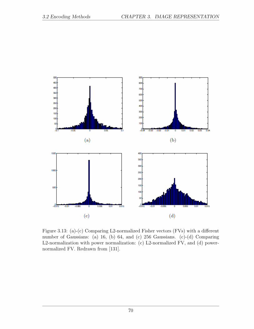
3.2 Encoding Methods CHAPTER 3. IMAGE REPRESENTATION
Figure 3.13: (a)-(c) Comparing L2-normalized Fisher vectors (FVs) with a differentnumber of Gaussians: (a) 16, (b) 64, and (c) 256 Gaussians. (c)-(d) ComparingL2-normalization with power normalization: (c) L2-normalized FV, and (d) power-normalized FV. Redrawn from [131].
70
3.2 Encoding Methods CHAPTER 3. IMAGE REPRESENTATION
3.2.3 Pooling and Normalization
Some algorithms face too much repeated data or inconsistent representations of thedata. Thus, further processing is needed to reduce and stabilize the data throughpooling and normalization. Here, some common pooling and normalization oper-ations that appear at the encoding stage are examined. Their role and effects invarious quantization methods will be discussed as well.
Pooling
Processing responses of all features can be expensive. Thus, the statistics of the fea-tures can be aggregated (or pooled) at various regions to yield a summary statistic(e.g. histogram). These summary statistics tend to be much lower in dimension andprevents over-fitting of the data. Furthermore, data with large variations can becondensed into a more compact representation by either removing or weighing theoutliers less. Thus, an ideal pooling method must preserve important informationand discard irrelevant materials while allowing invariance to small transformations ofthe input [18]. Typical pooling methods include: max-, sum-, and average-pooling.The feature with the largest response is chosen in max-pooling, and the responses arecombined additively or averaged in sum-pooling and average-pooling, respectively.The appropriate pooling operation depends on the sampling method, features type,and codebook size [18]. Max-pooling is the preferred method for sparsely sampledfeatures [18, 150].
Although max-, sum-, and average-pooling are simple ways to aggregate data,they have some obvious drawbacks. Responses that are slightly weaker than thestrongest are discarded in max-pooling even though their weaker responses couldprovide additional useful information. Every response within a region is consideredin sum- and average-pooling with equal importance, which would be undesirablesince the responses with low magnitudes can down weight the responses with highmagnitudes. Consequently, instead of considering one or all responses in a region,a probabilistic form of average-pooling and a weighted response can be consideredduring training and testing phases, respectively, as in stochastic pooling [222]. Theprobabilities and the weights in stochastic pooling are determined by the magnitudewith respect to other responses within the region (see Figure 3.14c). Alternatively,other mixture of pooling methods (e.g. taking the max over the fraction of all avail-able feature points) can sometimes yield more accurate results [18].
The aforementioned pooling techniques aggregate data over some pre-definedregion disregarding spatial layout and temporal order. At a global scale, spatialinvariance can be beneficial since the location of an action within a video shouldnot change the class of an action. However, the spatial layout at a local scale, suchas shape and location of body parts with respect to each part, can provide crucialinformation [127]. Motivated by the fact that varying spatial scale retains the orderof the features in locally orderless images (or histograms) [80], spatial pyramid pool-
71
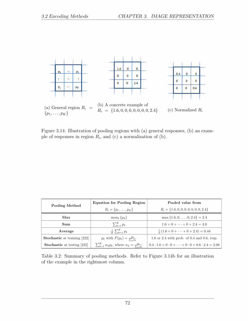
3.2 Encoding Methods CHAPTER 3. IMAGE REPRESENTATION
(a) General region Ri ={p1, . . . , pK}
(b) A concrete example ofRi = {1.6, 0, 0, 0, 0, 0, 0, 0, 2.4} (c) Normalized Ri
Figure 3.14: Illustration of pooling regions with (a) general responses, (b) an exam-ple of responses in region Ri, and (c) a normalization of (b).
Pooling MethodEquation for Pooling Region Pooled value from
Ri = {p1, . . . , pK} Ri = {1.6, 0, 0, 0, 0, 0, 0, 0, 2.4}
Max maxk {pk} max {1.6, 0, . . . , 0, 2.4} = 2.4
Sum∑K
k=1 pk 1.6 + 0 + · · ·+ 0 + 2.4 = 4.0
Average 1K
∑Kk=1 pk
19
(1.6 + 0 + · · ·+ 0 + 2.4) = 0.44
Stochastic at training [222] pk with P (pk) = pk∑k pk
1.6 or 2.4 with prob. of 0.4 and 0.6, resp.
Stochastic at testing [222]∑K
k=1wkpk, where wk = pk∑k pk
0.4 · 1.6 + 0 · 0 + · · ·+ 0 · 0 + 0.6 · 2.4 = 2.08
Table 3.2: Summary of pooling methods. Refer to Figure 3.14b for an illustrationof the example in the rightmost column.
72
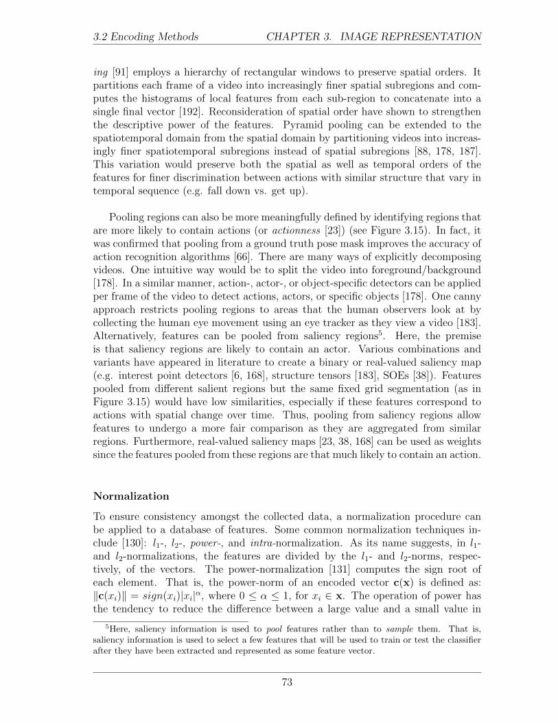
3.2 Encoding Methods CHAPTER 3. IMAGE REPRESENTATION
ing [91] employs a hierarchy of rectangular windows to preserve spatial orders. Itpartitions each frame of a video into increasingly finer spatial subregions and com-putes the histograms of local features from each sub-region to concatenate into asingle final vector [192]. Reconsideration of spatial order have shown to strengthenthe descriptive power of the features. Pyramid pooling can be extended to thespatiotemporal domain from the spatial domain by partitioning videos into increas-ingly finer spatiotemporal subregions instead of spatial subregions [88, 178, 187].This variation would preserve both the spatial as well as temporal orders of thefeatures for finer discrimination between actions with similar structure that vary intemporal sequence (e.g. fall down vs. get up).
Pooling regions can also be more meaningfully defined by identifying regions thatare more likely to contain actions (or actionness [23]) (see Figure 3.15). In fact, itwas confirmed that pooling from a ground truth pose mask improves the accuracy ofaction recognition algorithms [66]. There are many ways of explicitly decomposingvideos. One intuitive way would be to split the video into foreground/background[178]. In a similar manner, action-, actor-, or object-specific detectors can be appliedper frame of the video to detect actions, actors, or specific objects [178]. One cannyapproach restricts pooling regions to areas that the human observers look at bycollecting the human eye movement using an eye tracker as they view a video [183].Alternatively, features can be pooled from saliency regions5. Here, the premiseis that saliency regions are likely to contain an actor. Various combinations andvariants have appeared in literature to create a binary or real-valued saliency map(e.g. interest point detectors [6, 168], structure tensors [183], SOEs [38]). Featurespooled from different salient regions but the same fixed grid segmentation (as inFigure 3.15) would have low similarities, especially if these features correspond toactions with spatial change over time. Thus, pooling from saliency regions allowfeatures to undergo a more fair comparison as they are aggregated from similarregions. Furthermore, real-valued saliency maps [23, 38, 168] can be used as weightssince the features pooled from these regions are that much likely to contain an action.
Normalization
To ensure consistency amongst the collected data, a normalization procedure canbe applied to a database of features. Some common normalization techniques in-clude [130]: l1-, l2-, power-, and intra-normalization. As its name suggests, in l1-and l2-normalizations, the features are divided by the l1- and l2-norms, respec-tively, of the vectors. The power-normalization [131] computes the sign root ofeach element. That is, the power-norm of an encoded vector c(x) is defined as:‖c(xi)‖ = sign(xi)|xi|α, where 0 ≤ α ≤ 1, for xi ∈ x. The operation of power hasthe tendency to reduce the difference between a large value and a small value in
5Here, saliency information is used to pool features rather than to sample them. That is,saliency information is used to select a few features that will be used to train or test the classifierafter they have been extracted and represented as some feature vector.
73
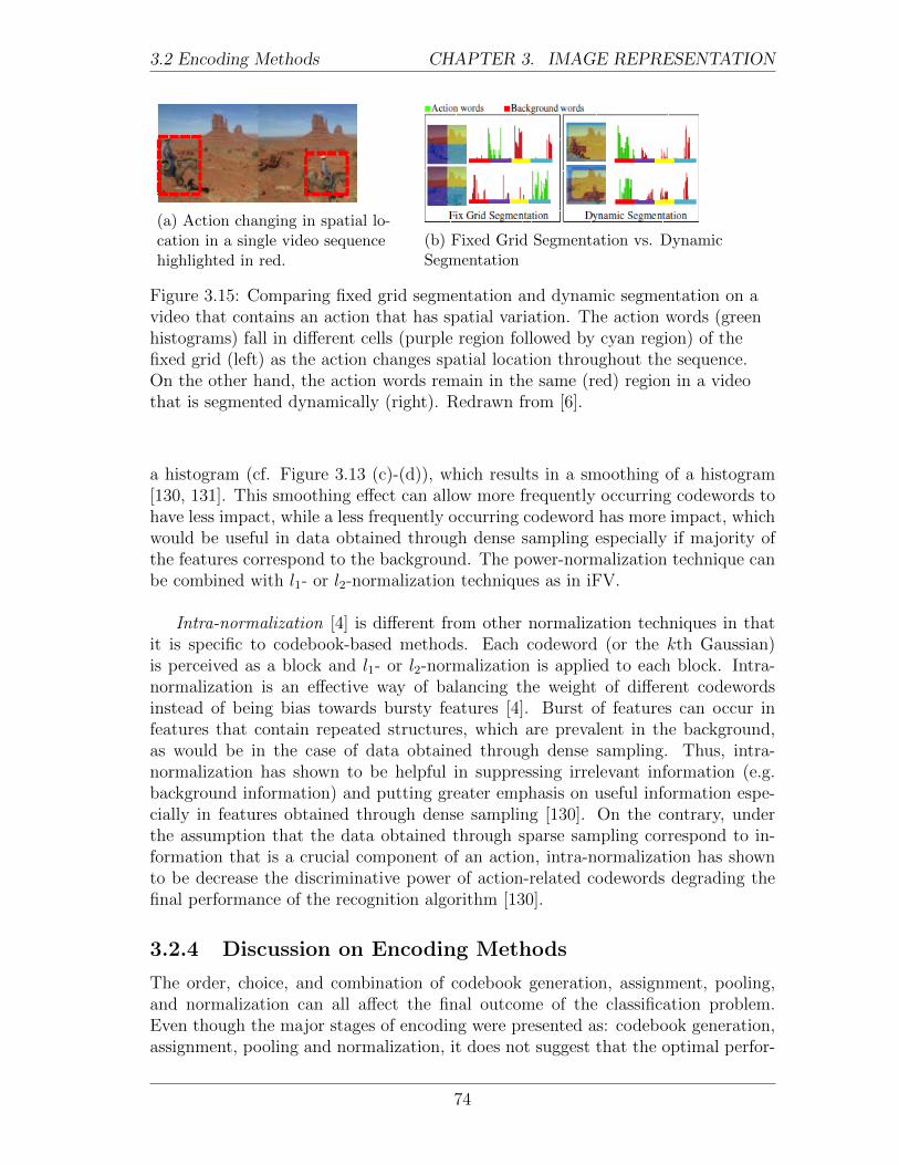
3.2 Encoding Methods CHAPTER 3. IMAGE REPRESENTATION
(a) Action changing in spatial lo-cation in a single video sequencehighlighted in red.
(b) Fixed Grid Segmentation vs. DynamicSegmentation
Figure 3.15: Comparing fixed grid segmentation and dynamic segmentation on avideo that contains an action that has spatial variation. The action words (greenhistograms) fall in different cells (purple region followed by cyan region) of thefixed grid (left) as the action changes spatial location throughout the sequence.On the other hand, the action words remain in the same (red) region in a videothat is segmented dynamically (right). Redrawn from [6].
a histogram (cf. Figure 3.13 (c)-(d)), which results in a smoothing of a histogram[130, 131]. This smoothing effect can allow more frequently occurring codewords tohave less impact, while a less frequently occurring codeword has more impact, whichwould be useful in data obtained through dense sampling especially if majority ofthe features correspond to the background. The power-normalization technique canbe combined with l1- or l2-normalization techniques as in iFV.
Intra-normalization [4] is different from other normalization techniques in thatit is specific to codebook-based methods. Each codeword (or the kth Gaussian)is perceived as a block and l1- or l2-normalization is applied to each block. Intra-normalization is an effective way of balancing the weight of different codewordsinstead of being bias towards bursty features [4]. Burst of features can occur infeatures that contain repeated structures, which are prevalent in the background,as would be in the case of data obtained through dense sampling. Thus, intra-normalization has shown to be helpful in suppressing irrelevant information (e.g.background information) and putting greater emphasis on useful information espe-cially in features obtained through dense sampling [130]. On the contrary, underthe assumption that the data obtained through sparse sampling correspond to in-formation that is a crucial component of an action, intra-normalization has shownto be decrease the discriminative power of action-related codewords degrading thefinal performance of the recognition algorithm [130].
3.2.4 Discussion on Encoding Methods
The order, choice, and combination of codebook generation, assignment, pooling,and normalization can all affect the final outcome of the classification problem.Even though the major stages of encoding were presented as: codebook generation,assignment, pooling and normalization, it does not suggest that the optimal perfor-
74
3.2 Encoding Methods CHAPTER 3. IMAGE REPRESENTATION
mance will be attained by following this exact sequence of steps. In fact, poolingand/or normalization can appear at any stage of encoding, if either or both stagesare deemed helpful at all.
It was mentioned in the codebook generation section that increasing the sizeof the codebook (i.e. the number of codewords) to a certain point improves theaccuracy of the recognition. Furthermore, it was pointed out that soft contrastingassignment methods retain richer information between codewords and feature vec-tors (e.g. dissimilarities between features and codewords). Together, they allow softcontrasting assignment methods to allow for a smaller codebook than other assign-ment models to achieve a similar level of performance [130].
In the normalization section, it was briefly discussed that power-normalizationhas a smoothing effect on histograms. When power-normalization is combined withsum- or average-pooling, a very good result can be obtained since sum-pooling pro-duces sharp and unbalanced histogram. Thus, the smoothening effect of power-normalization and the sharpening effect of sum-pooling pair well together to balancethe smooth-sharp effects. Noting that FVs are based on a codebook constructed us-ing GMMs, FVs implicitly perform an average pooling as it computes the first-orderstatistics to obtain the FV. As a result, FVs have been shown to perform well withaverage-pooling [39]. Consequently, power-normalization is the most well-suited nor-malization method with FVs [131].
A synergistic relationship can be observed between a well-chosen pair of assign-ment and pooling methods. For assignment models that pursue a sparse representa-tion, the optimal pooling method is via max-pooling [150]. Max-pooling couples wellwith sparse data since the distance between the nearest codeword and the featurevector is significantly closer than with other codewords inducing a strong response.The strong response is preserved and weaker responses are discarded through max-pooling [58]. In fact, it was empirically confirmed that SpC, an assignment modelthat pursues a sparse representation, and LLC, an assignment method that eventu-ally leads to sparsity through its locality constraint, is best pooled via max-pooling[192, 210].
Another factor that cannot be overlooked when choosing the type of encodingis the type of classifier in the subsequent step. That is, to use a linear SVM overnon-linear SVMs for its efficiency and smaller memory requirement, l2-normalizationwould be the preferred normalization method since the inner product of any vectorwith itself is an identity in l2-normalization, which ensures that the vector com-pared to itself is the most similar. This trait warrants stability during training[130, 192]. Thus, although the sharp characteristic induced by l2-normalization onFVs can be resolved via l1-normalization, power-normalization is preferred since l1-normalization suggests the use of non-linear SVMs as opposed to linear SVMs inthe succeeding classification step [131].
75
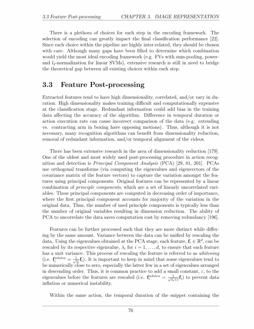
3.3 Feature Post-processing CHAPTER 3. IMAGE REPRESENTATION
There is a plethora of choices for each step in the encoding framework. Theselection of encoding can greatly impact the final classification performance [22].Since each choice within the pipeline are highly inter-related, they should be chosenwith care. Although many gaps have been filled to determine which combinationwould yield the most ideal encoding framework (e.g. FVs with sum-pooling, power-and l2-normalization for linear SVMs), extensive research is still in need to bridgethe theoretical gap between all existing choices within each step.
3.3 Feature Post-processing
Extracted features tend to have high dimensionality, correlated, and/or vary in du-ration. High dimensionality makes training difficult and computationally expensiveat the classification stage. Redundant information could add bias in the trainingdata affecting the accuracy of the algorithm. Difference in temporal duration oraction execution rate can cause incorrect comparison of the data (e.g. extendingvs. contracting arm in boxing have opposing motions). Thus, although it is notnecessary, many recognition algorithms can benefit from dimensionality reduction,removal of redundant information, and/or temporal alignment of the videos.
There has been extensive research in the area of dimensionality reduction [179].One of the oldest and most widely used post-processing procedure in action recog-nition and detection is Principal Component Analysis (PCA) [29, 81, 201]. PCAsuse orthogonal transforms (via computing the eigenvalues and eigenvectors of thecovariance matrix of the feature vectors) to capture the variation amongst the fea-tures using principal components. Original features can be represented by a linearcombination of principle components, which are a set of linearly uncorrelated vari-ables. These principal components are computed in decreasing order of importance,where the first principal component accounts for majority of the variation in theoriginal data. Thus, the number of used principle components is typically less thanthe number of original variables resulting in dimension reduction. The ability ofPCA to uncorrelate the data saves computation cost by removing redundancy [196].
Features can be further processed such that they are more distinct while differ-ing by the same amount. Variance between the data can be unified by rescaling thedata. Using the eigenvalues obtained at the PCA stage, each feature, fi ∈ Rd, can berescaled by its respective eigenvalue, λi for i = 1, . . . , d, to ensure that each featurehas a unit variance. This process of rescaling the feature is referred to as whitening(i.e. fwhiteni = 1√
λifi). It is important to keep in mind that some eigenvalues tend to
be numerically close to zero, especially the latter few in a set of eigenvalues arrangedin descending order. Thus, it is common practice to add a small constant, ε, to theeigenvalues before the features are rescaled (i.e. fwhiteni = 1√
λi+εfi) to prevent data
inflation or numerical instability.
Within the same action, the temporal duration of the snippet containing the
76
3.4 Final Remarks CHAPTER 3. IMAGE REPRESENTATION
single action can vary due to variations in action execution rate or different framerate of videos. Dynamic time warping (DTW) can be used to align sequences withvariable durations [60, 94, 101, 182]. DTW aligns the two time series by warping thetime axes to align the samples to the corresponding points. It simultaneously takesinto account a pairwise distance between corresponding frames and the sequencealignment cost using dynamic programming. A low alignment cost results when thetwo sequences are segmented similarly in time and performed at similar rates.
Post-processing is not necessary for all methods and is seldom done on manyencoding methods other than FV-based methods [130]. However, empirical evalua-tions show that applying PCA-whitening greatly improves algorithms that do notusually apply PCA-whitening, such as VQ and LLC-encoded methods [130].
3.4 Final Remarks
In this chapter, three major steps that are involved in representing images wereexamined: feature extraction, feature encoding, and feature post-processing. Thefeature extraction stage and the encoding stage can occur once or multiple times asneeded before it enters the final classification stage [67, 123]. Furthermore, althoughdimensionality reduction may improve the accuracy and efficiency of an algorithm,it is not a necessary procedure and can occur before or after the encoding stage.
77
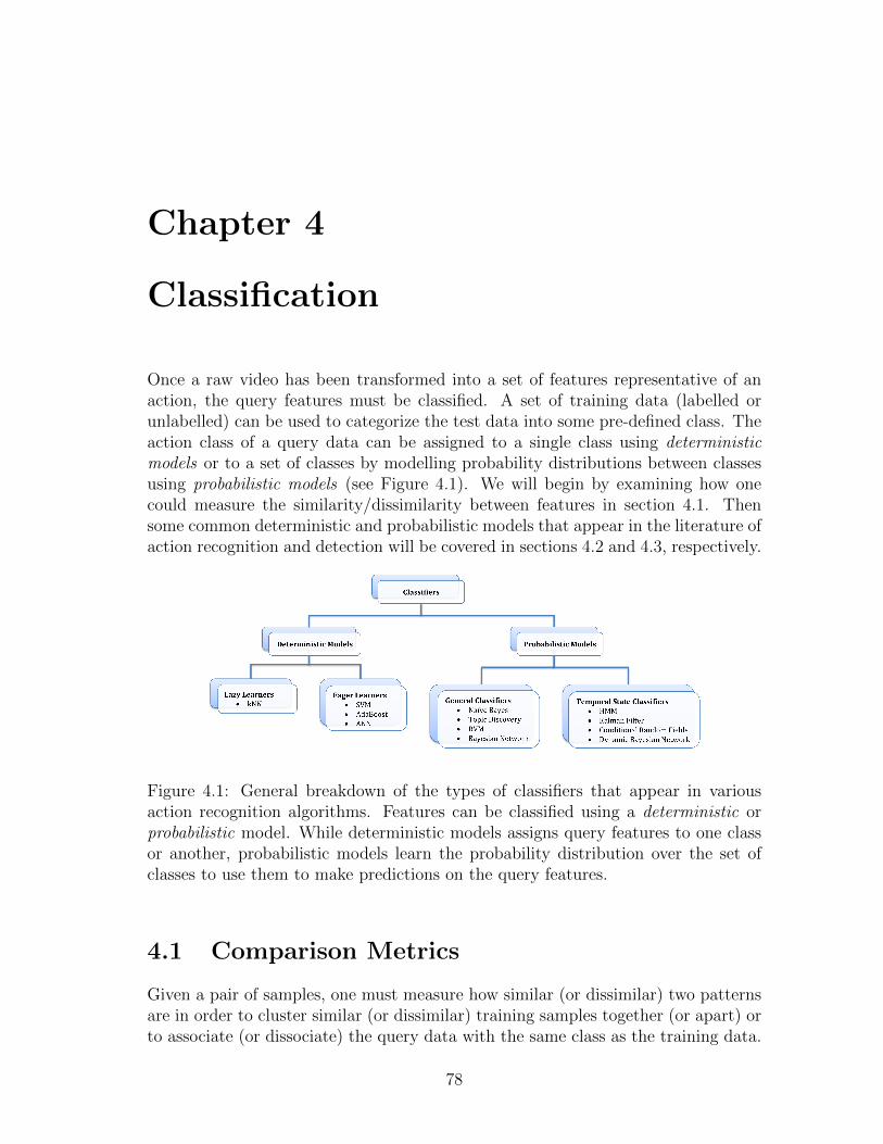
Chapter 4
Classification
Once a raw video has been transformed into a set of features representative of anaction, the query features must be classified. A set of training data (labelled orunlabelled) can be used to categorize the test data into some pre-defined class. Theaction class of a query data can be assigned to a single class using deterministicmodels or to a set of classes by modelling probability distributions between classesusing probabilistic models (see Figure 4.1). We will begin by examining how onecould measure the similarity/dissimilarity between features in section 4.1. Thensome common deterministic and probabilistic models that appear in the literature ofaction recognition and detection will be covered in sections 4.2 and 4.3, respectively.
Figure 4.1: General breakdown of the types of classifiers that appear in variousaction recognition algorithms. Features can be classified using a deterministic orprobabilistic model. While deterministic models assigns query features to one classor another, probabilistic models learn the probability distribution over the set ofclasses to use them to make predictions on the query features.
4.1 Comparison Metrics
Given a pair of samples, one must measure how similar (or dissimilar) two patternsare in order to cluster similar (or dissimilar) training samples together (or apart) orto associate (or dissociate) the query data with the same class as the training data.
78
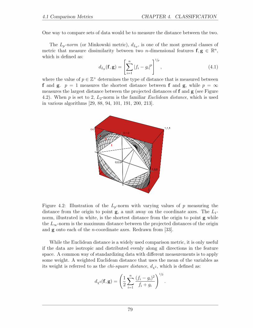
4.1 Comparison Metrics CHAPTER 4. CLASSIFICATION
One way to compare sets of data would be to measure the distance between the two.
The Lp-norm (or Minkowski metric), dLp , is one of the most general classes ofmetric that measure dissimilarity between two n-dimensional features f ,g ∈ Rn,which is defined as:
dLp(f ,g) =
[n∑i=1
|fi − gi|p]1/p
, (4.1)
where the value of p ∈ Z+ determines the type of distance that is measured betweenf and g. p = 1 measures the shortest distance between f and g, while p = ∞measures the largest distance between the projected distances of f and g (see Figure4.2). When p is set to 2, L2-norm is the familiar Euclidean distance, which is usedin various algorithms [29, 88, 94, 101, 191, 200, 213].
Figure 4.2: Illustration of the Lp-norm with varying values of p measuring thedistance from the origin to point g, a unit away on the coordinate axes. The L1-norm, illustrated in white, is the shortest distance from the origin to point g whilethe L∞-norm is the maximum distance between the projected distances of the originand g onto each of the n-coordinate axes. Redrawn from [33].
While the Euclidean distance is a widely used comparison metric, it is only usefulif the data are isotropic and distributed evenly along all directions in the featurespace. A common way of standardizing data with different measurements is to applysome weight. A weighted Euclidean distance that uses the mean of the variables asits weight is referred to as the chi-square distance, dχ2 , which is defined as:
dχ2(f ,g) =
(1
2
n∑i=1
(fi − gi)2
fi + gi
)1/2
.
79

4.1 Comparison Metrics CHAPTER 4. CLASSIFICATION
Alternatively, correlated data with varying scales can be accommodated by con-sidering the covariance as in the Mahalanobis distance, dM , which is defined as:
dM(f ,g) =[(f − g)Σ−1(f − g)>
]1/2,
where Σ is the covariance matrix corresponding to the typical distribution of interestpoints in the training data [87]. Thus, when the data is scattered in all directionsaround the centre of the cluster, the convariance matrix is a diagonal matrix, whichis the normalized Euclidean distance and an identity covariance matrix would bethe standard normalized Euclidean distance. The Mahalanobis distance provides auseful measure to calculate the amount of separation between two classes of features(e.g. Hu moments [16] or Fourier projections of MHVs [201]) by measuring the dis-tance between their respective centres [31].
There are various comparison metrics that measure the difference (or similarity)of two probability distributions. The Kullback-Leibler (KL) distance, dKL, whichmeasures the difference between two probability distributions, is defined as:
dKL(f ,g) =n∑i=1
fi · ln(figi
).
The KL distance is nonzero and is equal to zero if and only if f = g [33]. KLdistance is used in various action recognition algorithms [96, 123]. KL distance lackssymmetry (i.e. dKL(f ,g) 6= dKL(g, f)), which is undesirable in action recognitionalgorithms because two features should be equally similar or dissimilar to be (partof) an action regardless of the order of comparison (i.e. action a is similar to action bas much as action b is similar to action a). Asymmetry can be overcome by redefiningthe KL distance as d′KL(f ,g) = dKL(f ,g) + dKL(g, f) [123]. Alternatively, the KLdistance can be modified into:
dJ(f ,g) =n∑i=1
(fi − gi)(ln fi − ln gi),
referred to as the Jeffreys divergence, which is numerically stable, symmetric, androbust to noise [134, 144].
The Bhattacharyya coefficient, dB, which measures the overlap between two prob-ability distributions is defined as:
dB(f ,g) =n∑i=1
[fi · gi]1/2.
The Bhattacharyya coefficient, which is not to be confused with the Bhattacharyyadistance, is bounded below by zero and above by one. Zero indicates no overlap andone indicates a perfect match between two normalized distributions f and g. Thebounded nature of the Bhattacharyya coefficient makes the measure robust to small
80

4.1 Comparison Metrics CHAPTER 4. CLASSIFICATION
outliers, which is favourable in action recognition application due to occlusion thatcould affect the overall distribution [28, 211].
The partial matches between two histograms in their corresponding bins can bemodelled using a histogram intersection (HI) [172]. Histogram Intersection (HI)[172], dHI , is defined as:
dHI(f ,g) = 1−∑n
i=1 min (fi, gi)∑ni=1 fi
.
Interestingly, when the two histograms have the same size (i.e.∑
i fi =∑
i gi), thenthe histogram intersection of f and g is equivalent to the normalized L1-distance[172].
So far, all the measures that were mentioned in this section measured the sim-ilarity (or dissimilarity) between histograms bin-to-bin (i.e. compare fi and gi ∀ ibut never fi and gj for i 6= j). This forces the two histograms to have the samebin sizes, which could cause the histogram to lack the discriminating power due tocoarse binning or grouping of similar features due to fine binning. Thus, the flexi-bility for histograms to have different sizes and the ability to compare them acrossbins could be more robust and more useful [144].
The Earth Mover’s distance (EMD) [143] is a cross-bin comparison metric thatcomputes the minimal amount of work needed to transform one distribution to an-other. EMD can be broken down into a two-step process: (i) given two distributions,f ∈ Rm and g ∈ Rn, find the flow with the smallest overall cost of transferring thedistributional masses from f to g (or from g to f), then (ii) use the flow to determinethe amount of work required to transfer the distribution masses. To find the optimalflow, φ∗, is to solve the following transportation problem:
φ∗ = arg minφij
m∑i=1
n∑j=1
φijδij, (4.2)
where φij is the flow between fi and gj for 1 ≤ i ≤ m, 1 ≤ j ≤ n, and δij is the“ground distance” between fi and gj ∀ i, j, which can be any distance measurebetween single elements (e.g. L1-norm [144], L2-norm [144, 218]) depending on thefeatures. Since (4.2) is a transportation problem (see Figure 4.3), the optimal flow,φ∗, can be found using linear programming [144]. Then the EMD between twohistograms, f and g, is defined as the work normalized by the total flow:
dEMD(f ,g) =
∑mi
∑nj=1 φ
∗ijδij∑m
i=1
∑nj=1 φ
∗ij
,
where the normalization factor (total flow) is equivalent to the total weight of thesmaller distribution, which prevents the measure from favouring the smaller distri-bution [144].
81

4.1 Comparison Metrics CHAPTER 4. CLASSIFICATION
(a) Transportation Problem
(b) Solution to the Transportation Problem
Figure 4.3: Example of the Earth Mover’s Distance (EMD). To calculate the EMDof f = [0.4 0.2 0.2 0.1 0.1]> and g = [0.6 0.2 0.1]>, (a) convert f and g into a trans-portation problem, where the cost (or ground distance), δij between fi and gj for1 ≤ i ≤ m, 1 ≤ j ≤ n is pre-defined. (b) The optimal flow φ∗ of the transporta-tion problem is found through linear programming. The columns of optimal flow,φ∗ = [φ1 φ2 φ3], represents the amount of flow φ3 that is transferred from node φ2
to node φ1. dEMD(f ,g) = 0.2·0+0.3·3+0.1·1+0.1·4+0.1·1+0·5+0.1·20.2+0.3+0.1+0.1+0.1+0.1
= 1.70.9
= 1.8889.
82
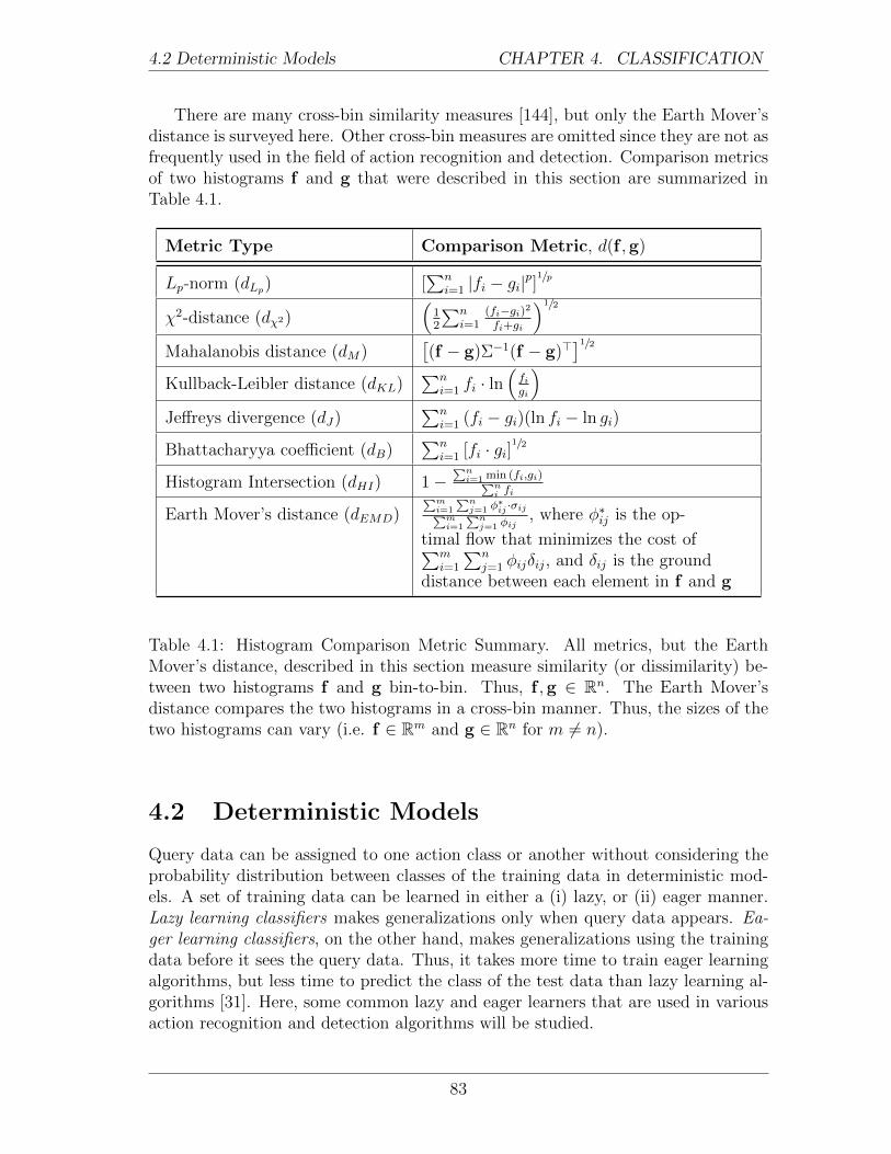
4.2 Deterministic Models CHAPTER 4. CLASSIFICATION
There are many cross-bin similarity measures [144], but only the Earth Mover’sdistance is surveyed here. Other cross-bin measures are omitted since they are not asfrequently used in the field of action recognition and detection. Comparison metricsof two histograms f and g that were described in this section are summarized inTable 4.1.
Metric Type Comparison Metric, d(f ,g)
Lp-norm (dLp) [∑n
i=1 |fi − gi|p]
1/p
χ2-distance (dχ2)(
12
∑ni=1
(fi−gi)2fi+gi
)1/2
Mahalanobis distance (dM)[(f − g)Σ−1(f − g)>
]1/2Kullback-Leibler distance (dKL)
∑ni=1 fi · ln
(figi
)Jeffreys divergence (dJ)
∑ni=1 (fi − gi)(ln fi − ln gi)
Bhattacharyya coefficient (dB)∑n
i=1 [fi · gi]1/2
Histogram Intersection (dHI) 1−∑ni=1 min (fi,gi)∑n
i fi
Earth Mover’s distance (dEMD)∑mi=1
∑nj=1 φ
∗ij ·σij∑m
i=1
∑nj=1 φij
, where φ∗ij is the op-
timal flow that minimizes the cost of∑mi=1
∑nj=1 φijδij, and δij is the ground
distance between each element in f and g
Table 4.1: Histogram Comparison Metric Summary. All metrics, but the EarthMover’s distance, described in this section measure similarity (or dissimilarity) be-tween two histograms f and g bin-to-bin. Thus, f ,g ∈ Rn. The Earth Mover’sdistance compares the two histograms in a cross-bin manner. Thus, the sizes of thetwo histograms can vary (i.e. f ∈ Rm and g ∈ Rn for m 6= n).
4.2 Deterministic Models
Query data can be assigned to one action class or another without considering theprobability distribution between classes of the training data in deterministic mod-els. A set of training data can be learned in either a (i) lazy, or (ii) eager manner.Lazy learning classifiers makes generalizations only when query data appears. Ea-ger learning classifiers, on the other hand, makes generalizations using the trainingdata before it sees the query data. Thus, it takes more time to train eager learningalgorithms, but less time to predict the class of the test data than lazy learning al-gorithms [31]. Here, some common lazy and eager learners that are used in variousaction recognition and detection algorithms will be studied.
83

4.2 Deterministic Models CHAPTER 4. CLASSIFICATION
4.2.1 Lazy Learners
Lazy-based learning classifiers defer data processing until they receive a request toclassify an unlabelled test example [31]. The classifier waits for query data beforeit makes any generalizations about the data. One common lazy learning classifierused in action recognition is the k-nearest neighbour (kNN) classifier [94, 124]. Itdetermines the class of the test sample by growing a spherical region centred at thesample until the region contains k ∈ Z+ training data. The test data is labelled bythe class with the majority vote in the enclosed space (see Figure 4.4) [31]. Manyearlier algorithms set k = 1, to find the nearest neighbour (i.e. template) to thequery (i.e. test) vector [34, 94]. The distance between the training set and the testdata can be obtained via a comparison metric mentioned in the previous section.Thus, computing can be expensive with a large training set. When there are twoclasses in the training set, an odd k value is used to avoid ties between the classes.With more classes, larger k values are used since they are more likely to break theties [31]. Although the kNN classifier is simple to implement, it is prone to localnoise. Furthermore, with an increase in the number of features, more training datais required leading to the case of curse of dimensionality. To avoid bias when thereare an unbalanced amount of training data from different classes or to assign moreweight on false negatives over false positives, the standard kNN algorithm can bemodified to assign a particular class to the test data if at least l of the k nearestneighbours are in that class for l < k [31].
Figure 4.4: k-nearest neighbours with k = 5. A circular region (red) centred aroundthe test sample (star) is expanded until k = 5 samples (circles and triangles) arecontained within the circular region. The test sample is labelled as the same class astriangle since there are more triangles (3) than circles (2) inside the bound region.
84

4.2 Deterministic Models CHAPTER 4. CLASSIFICATION
4.2.2 Eager Learners
Given a collection of training data, eager learning classifiers learn a model thatwould generalize the data as soon as it becomes available before the test data mustbe categorized. A model can be generated by partitioning the feature space of thedata into a set of decision regions (see Figure 4.5) [31]. These regions provide aguideline to classify the query feature into one of the classes. The decision regionsare separated by decision boundaries, which can be described by a set of discrimi-nant functions. Some eager learning algorithms that are commonly used in actionrecognition and detection algorithms include: support vector machines (SVMs), Ad-aBoost, and artificial neural networks (ANNs).
(a) Linearly separable data (b) Non-linearly separable data
Figure 4.5: Decision Boundaries. Red lines indicate the decision boundary, whichseparates the samples of different classes (triangles and circles) into decision regions.(a) A linear decision boundary is the simplest decision boundary, which can bedescribed by a linear (discriminant) function. (b) A non-linear decision boundarycan be obtained with a set of complex polynomials.
A support vector machine (SVM) is one of the most common supervised classi-fication tools used in action recognition and detection, e.g. [63, 67, 69, 82, 88, 103,107, 137, 147, 170, 173, 190, 186, 188, 211, 226]. An SVM is trained to find a hyper-plane (or a decision boundary) that separates labelled data from two classes into itsrespective groups. The best hyperplane is the one that separates the two classes withthe largest distance between the nearest point from each class to the hyperplane (seeFigure 4.6). Since action recognition involves classifying videos into multiple actions(classes), a multi-class SVM must be employed, which can be done by applying theone-versus-all approach [88, 225]. The one-versus-all approach takes the trainingdata from class k labelled as positive and the rest as negative examples to train thekth model. Kernels enable implicit operation in a higher dimensional feature space,where hyperplane separability may be possible. There are two types of kernels: (i)linear, and (ii) non-linear. To determine what would be an appropriate kernel forthe algorithm, one should examine the ratio between the number of features andthe training data. A linear kernel is preferred when the number of features is large(i.e. high dimensional feature space) (e.g. DT/iDT features) relative to the number
85

4.2 Deterministic Models CHAPTER 4. CLASSIFICATION
of training samples to prevent over-fitting in the feature space. When there are afew features with a lot of samples, a non-linear kernel would be a better choice. Al-though non-linear kernels typically achieve a lower error rate, linear SVMs are lesscomputationally expensive and require less storage than non-linear SVMs allowingreal-time detections possible [26, 210]. By adding more features, a linear SVM canbe used.
Figure 4.6: Support Vector Machine (SVM). Solid lines indicate the decision bound-ary separating the samples of different classes (triangles and circles). Dashed linesare lines parallel to the decision boundary closest to the data of one class. SVMseeks a line that would maximize the margin, the distance between the dashed andsolid line (i.e. red line).
Adaptive Boosting (AdaBoost) is a learning algorithm that takes several weakclassifiers, classifiers that are slightly better than random guessing, and constructsa meta-classifier. By assigning different weights to training samples, different clas-sifiers would pay more attention to different samples. The weights of an individualclassifier is assigned depending on its accuracy [23]. This approach has been appliedwith some success in various action recognition algorithms [36, 89, 96, 124].
Artificial neural networks (ANNs) are another widely used classification algo-rithm. The artificial neuron (perceptron, or more generally referred to as units)in each layer computes the weighted sum of its inputs. If the sum exceeds somespecified threshold, the unit outputs a value [31]. A unit models a linear discrim-inant function partitioning the feature space using a decision boundary. Using amultilayer network, nonlinearly separable functions can be learned (see Figure 4.7).The network is trained via backpropagation, which involves repeatedly presentingthe training data to the network and adjusting the weights in the network to ob-tain a desired output [31, 33]. The number of units in the hidden layers govern theexpressive power of the network [33]. A small number of hidden units is sufficient
86
4.3 Probabilistic Models CHAPTER 4. CLASSIFICATION
for well-separated or linearly separable patterns, but highly interspersed patternswith complicated densities require more hidden units. While a large number of hid-den units produces a discriminative network lessening the training error, trainingbecomes extremely time-consuming. Furthermore, it can lead to overfitting of thedata, causing random noise in the test data to be modelled and poor generalizationto the test data [31]. An ANN with too few hidden units would not have enoughparameters to fit the training data, yielding poor classification results on the testdata. Thus, finding an intermediate number of hidden units is key to obtaining goodclassification results with such powerful classification tool.
ANNs and CNNs (mentioned in Section 3.1.2) have very similar architectures.Both networks output class scores of a feature vector by processing the componentsof a feature vector into a sequence of input, hidden, and output layers [33]. Eachlayer consists of a set of units, where each unit in the hidden layer receives someinput, performs a dot product, and optionally follows it with a non-linearity. Basedon an assumption that input signals from the domain of interest (e.g. images) arelocally correlated (e.g. spatially neighbouring pixels), CNNs allow their receptivefields of the hidden units to have a relatively local support [93], while more generalANNs do not. This allows units in the hidden layers of a CNN to be connectedto a local neighbourhood of the previous layer, while all units in every layer of ageneral ANN is allowed to be fully-connected. Fewer connections between unitssignificantly reduces the number of parameters (weights) that must be learned [93].Consequently, fewer weights reduces the number of training that is required to coverthe space of possible variations. Furthermore, it reduces the amount of memoryrequired to store the weights in the hardware [93]. Remark, the last layers of atypical CNN architecture can be fully-connected. This allows for an output of aclass, a class probability, or features that can be fed into another classifier (e.g.SVM).
4.3 Probabilistic Models
Probabilistic models learn the probability distribution over the set of classes to de-termine the probability of the query data belonging to each action class. Theseprobabilistic models can be broadly categorized into two types: general classifiersand temporal state-space classifiers. General classifiers categorize features withoutexplicitly modelling variations in time while temporal state-space models use tem-poral order information of features. Here, we look at probabilistic models that fallunder general or temporal state-space models.
4.3.1 General Classifiers
The relationship between features and their respective action class can be modelledusing probabilities. Here, we examine some common general probabilistic modelsthat have been implemented in the field of action recognition, such as the naive
87

4.3 Probabilistic Models CHAPTER 4. CLASSIFICATION
(a) Two-Layer Neural Network
(b) Linear DecisionBoundary
(c) Multi-layer Neural Network
(d) Arbitrary De-cision Boundaries
Figure 4.7: Artificial Neural Networks (ANNs) with different number of layers.While a two-layer neural network classifier (4.7a) is only capable of implementinglinear decision boundaries (4.7b), a multi-layer neural network (4.7c) with an appro-priate number of hidden units can implement arbitrary decision boundaries (4.7d),which do not necessarily have to be convex nor simply connected. Adapted from[33].
88

4.3 Probabilistic Models CHAPTER 4. CLASSIFICATION
Bayes classifier, latent topic discovery models, relevance vector machines, and theBayesian network.
The naive Bayes classifier is one of the simplest probabilistic models that assignsa feature, x, to some action class c by comparing the posterior probability P (ck|x)∀ ck ∈ C [31]. Applying the Bayes’ rule, the conditional posterior probability canbe written as:
P (ck|x) =P (x|ck)P (ck)
P (x), (4.3)
where P (x|ck) represents the probability of feature x (e.g. filter bank [24]) belong-ing to class ck, P (ck) and P (x) represent probabilities of observing class ck andfeature x, respectively. P (x|ck), P (c), and P (x) can all be trained from observingthe distributions within the training set. The naive Bayes classifier makes a naiveassumption that the features are conditionally independent to one another given itsclass (i.e. P (x1, . . . , xn|ck) = P (x1|ck) . . . P (xn|ck)). Then the test feature x can beassigned to the class with the maximum a posterior probability P (c|x) [33], whichis formulated as
ck = arg maxck∈C
P (ck|x) =1
P (x)arg max
ck∈CP (x1|ck) . . . P (xn|ck)P (ck). (4.4)
Through the naive Bayes independence assumption, which may not necessarily betrue, naive Bayes classifier is a simple classifier that is a good candidate for imple-mentation for its simplicity and efficiency.
Latent topic discovery models are statistical models that were originally pop-ularized for the discovery of topics in a text. This approach can be extended todiscover any latent classes in a collection of data, such as actions in videos. Twolatent topic discovery models, probabilistic Latent Semantic Analysis (pLSA) [54]and Latent Dirichlet Allocation (LDA) [15], have commonly appeared in variousaction recognition algorithms [122, 191, 227] [122, 199]. pLSA and LDA model thedistribution of classes in sets of videos, such that the model can be used to classifythe latent topics (i.e. action classes) in the new videos. pLSA assumes that a videosequence, vi, and a feature, fj, are conditionally independent given an action class,ck, (see Figure 4.8a), then the action class of the test data v′ can be best describedby solving
c∗ = arg maxkP (ck|v′),
which can be computed using the EM algorithm [122]. To determine a model thatbest represents a mixture of actions that could occur in a single video, the most op-timal action proportion in videos, p(ck|vi) for i = 1, . . . , N , must be learned. pLSAlearns the class mixture probabilities by going through each video in the trainingset to describe the process of generating videos with action class distributions thatwas in some video in the set.
The pLSA approach enforces the model to be stringent, placing new (unseen)videos at points within the pre-defined action distribution, leading to an overfit
89
4.3 Probabilistic Models CHAPTER 4. CLASSIFICATION
model (see Figure 4.9) [15]. To overcome this stringency, LDA sets arbitrary topicproportions (a prior probability distribution) θi for each video vi. To ensure thatthe number of parameters to be learned does not grow linearly with the number ofvideos in the training set, the mixing proportions of actions per video are controlledby a parameter α, which is specified per set of videos (see Figure 4.8b). Then thejoint distribution of the action class mixture, θ, a set of classes c, and a set offeatures, f , is given by:
p(θ, c, f |α, β) = p(θ, α)K∏k=1
p(ck|θ)p(fn|ck, β),
where β parameterizes the distribution of the features within a particular actionlabel (i.e. β corresponds to p(fi|ck)). Parameters α and β are found using the EMalgorithm for a given collection of video sequences [15]. The feature fj is classifiedto be action c∗ if
c∗ = arg maxkp(ck|fj, α, β). (4.5)
Since the number of topics is fixed to a particular value in LDA, it prevents over-fitting from occurring, especially if a video contains a small amount of features totrain, since it can rely on the prior to give a more reasonable guess about the actionsfor that video [122]. Conversely, if videos are known to produce a large amount offeatures, then the data would dominate the priors. Finally, it is worth noting thatpLSA is more computationally efficient than LDA [108].
Relevance vector machines (RVMs) have an identical functional form as the de-terministic model, SVM. It finds a hyperplane that separates the relevance vectorsinto two classes. Different from SVMs, RVMs provide a probabilistic classificationinstead of a deterministic decision. Furthermore, the hyperplane separates relevancevectors, prototypical representations of classes (e.g. action class), instead of supportvectors (examples close to the decision boundary) [125]. RVMs tend to have a longertraining time than SVMs. However, since RVMs result in a sparser set of supportvectors, the computation time for test points is much less than on an SVM [13].
Some algorithms design probabilistic models using a Bayesian network suited toincorporate the necessary variables to recognize the action [35]. Using a graphicalrepresentation, a complex system can be decomposed into simpler parts to providea causal relationship between the variables. In addition, graphical models factorizevariables into several conditional probability distributions that are simpler to com-pute [100, 171, 174]. For example, Figure 4.10 suggests the following factorized jointprobability:
p(θ, x, y, a, b, s, δ) = p(σ)p(s|δ)p(y|x, s, δ)p(b|a, s, δ)p(a)p(θ)p(x|θ),
where θ, x, y, a, b, s, δ are parameters that indicate the centroid, position and veloc-ity of body parts, position and velocity of detections, appearance of body parts,appearance of a detection, map of body parts to detects, and detection of body
90
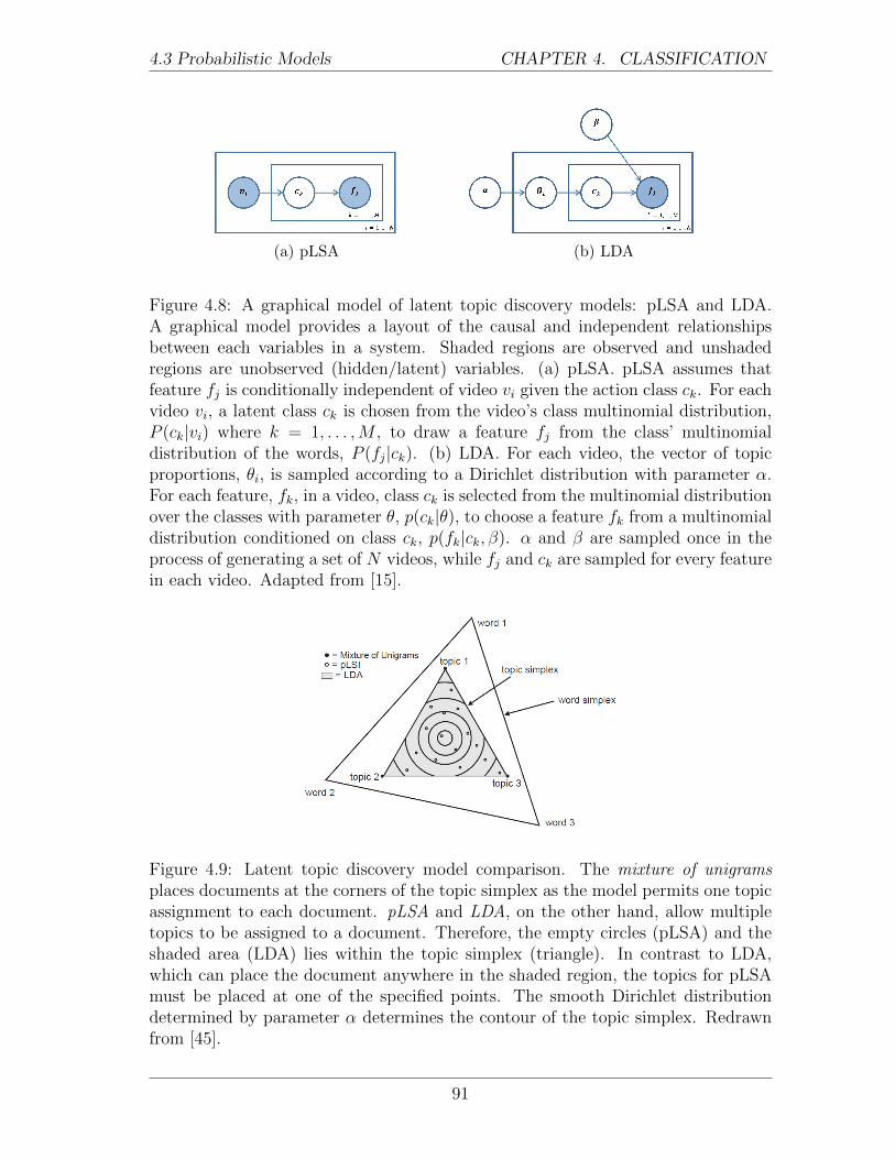
4.3 Probabilistic Models CHAPTER 4. CLASSIFICATION
(a) pLSA (b) LDA
Figure 4.8: A graphical model of latent topic discovery models: pLSA and LDA.A graphical model provides a layout of the causal and independent relationshipsbetween each variables in a system. Shaded regions are observed and unshadedregions are unobserved (hidden/latent) variables. (a) pLSA. pLSA assumes thatfeature fj is conditionally independent of video vi given the action class ck. For eachvideo vi, a latent class ck is chosen from the video’s class multinomial distribution,P (ck|vi) where k = 1, . . . ,M , to draw a feature fj from the class’ multinomialdistribution of the words, P (fj|ck). (b) LDA. For each video, the vector of topicproportions, θi, is sampled according to a Dirichlet distribution with parameter α.For each feature, fk, in a video, class ck is selected from the multinomial distributionover the classes with parameter θ, p(ck|θ), to choose a feature fk from a multinomialdistribution conditioned on class ck, p(fk|ck, β). α and β are sampled once in theprocess of generating a set of N videos, while fj and ck are sampled for every featurein each video. Adapted from [15].
Figure 4.9: Latent topic discovery model comparison. The mixture of unigramsplaces documents at the corners of the topic simplex as the model permits one topicassignment to each document. pLSA and LDA, on the other hand, allow multipletopics to be assigned to a document. Therefore, the empty circles (pLSA) and theshaded area (LDA) lies within the topic simplex (triangle). In contrast to LDA,which can place the document anywhere in the shaded region, the topics for pLSAmust be placed at one of the specified points. The smooth Dirichlet distributiondetermined by parameter α determines the contour of the topic simplex. Redrawnfrom [45].
91
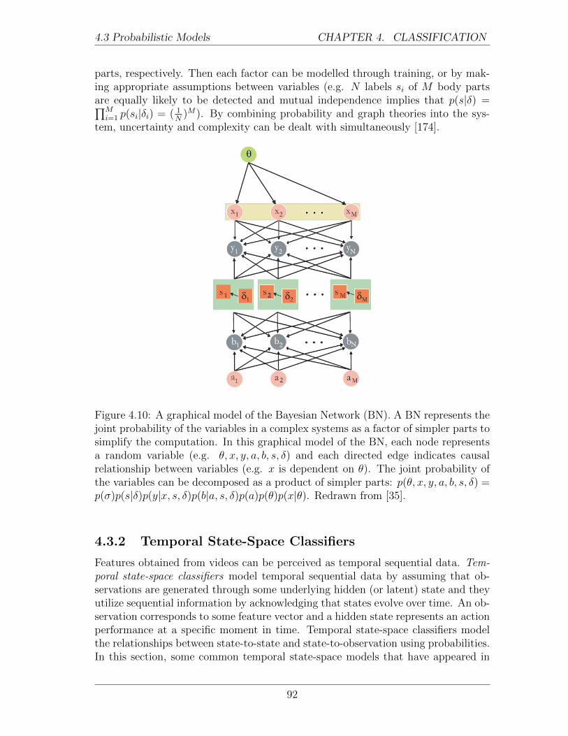
4.3 Probabilistic Models CHAPTER 4. CLASSIFICATION
parts, respectively. Then each factor can be modelled through training, or by mak-ing appropriate assumptions between variables (e.g. N labels si of M body partsare equally likely to be detected and mutual independence implies that p(s|δ) =∏M
i=1 p(si|δi) = ( 1N
)M). By combining probability and graph theories into the sys-tem, uncertainty and complexity can be dealt with simultaneously [174].
Figure 4.10: A graphical model of the Bayesian Network (BN). A BN represents thejoint probability of the variables in a complex systems as a factor of simpler parts tosimplify the computation. In this graphical model of the BN, each node representsa random variable (e.g. θ, x, y, a, b, s, δ) and each directed edge indicates causalrelationship between variables (e.g. x is dependent on θ). The joint probability ofthe variables can be decomposed as a product of simpler parts: p(θ, x, y, a, b, s, δ) =p(σ)p(s|δ)p(y|x, s, δ)p(b|a, s, δ)p(a)p(θ)p(x|θ). Redrawn from [35].
4.3.2 Temporal State-Space Classifiers
Features obtained from videos can be perceived as temporal sequential data. Tem-poral state-space classifiers model temporal sequential data by assuming that ob-servations are generated through some underlying hidden (or latent) state and theyutilize sequential information by acknowledging that states evolve over time. An ob-servation corresponds to some feature vector and a hidden state represents an actionperformance at a specific moment in time. Temporal state-space classifiers modelthe relationships between state-to-state and state-to-observation using probabilities.In this section, some common temporal state-space models that have appeared in
92
4.3 Probabilistic Models CHAPTER 4. CLASSIFICATION
the action recognition and detection literature will be reviewed.
An action can be perceived as a sequence of states that is directly influenced byits previous state(s), and each state of the action can be observed by some featurerepresentation. Correspondingly, a video of an action can be modelled using theHidden Markov Model (HMM), where each state of an action corresponds to thehidden/latent state, zt, with observation, ft (see Figure 4.11). Then the task ofaction recognition/detection can be formulated by finding the most probable set ofsequences, Z = {zt|t ∈ Z+}, that corresponds to a set of observations, F = {ft|t ∈Z+}. That is, maximize the joint probability of the paired observation and labelsequences:
P (c, f) =n∏t=1
P (zt|zt−1)P (ft|zt),
where P (zt|zt−1) and P (ft|zt) denote transition probabilities and emission probabil-ities, respectively, for t = 1, . . . , n. The transition probability models the probabilityof a state transitioning from zt−1 to zt, and the emission probability models the prob-ability of observation ft being emitted from state zt. Transition probabilities can betrained using k-means clustering [42, 135] for supervised data and the Baum-Welchalgorithm for unsupervised data [2, 61, 99, 200, 209]. Each HMM represents anaction category [61, 200, 209]. The observation can be of the entire body [2, 200], abody part [61, 135], or an interest point (e.g. mesh [42], HOG [99]). The probabilitythat a sequence of hidden states would yield a set of observations is referred to asthe decoding problem [33]. The most likely action class that the test data wouldbelong to among the c HMMs, where c denotes the number of action classes, can beevaluated using the Viterbi algorithm [2], or maximum likelihood estimation (MLE)[99]. Since HMMs are designed to deal with time-sequence data, they are robust totime scale shift and variance [209].
The features obtained from videos can be noisy and extracted at random inter-vals. The hidden state corresponding to noisy data does not need to be constrainedto discrete variables, but can be estimated as continuous variables using Kalmanfilters [202] [145]. A Kalman filter models each state variable as continuously dis-tributed using a Gaussian distribution [145]. Since the convolution and the productof a Gaussian also yields a Gaussian, all probabilities (transition and emission) arealso Gaussians. The Kalman filter works in a two-step process: the prediction stepand the correction step. At the prediction step, the Kalman filter estimates the cur-rent (hidden) state, zt, along with its uncertainties and the future state, zt+1. At thecorrection step, the weighted average of the new observation, ft+1, and the predictedvalue is used to update the new hidden state zt+1. The new hidden state is assignedwith more emphasis placed on the predicted value if the new observation is deemedunreliable (noisy), and the observation is more favoured if the process deem unpre-dictable and unreliable [145]. The prediction and correction phases run recursivelyto update the current estimate based on all of the past measurements. Kalman filtersare often used in conjunction with tracking-based algorithms [17, 32, 50]. Kalman
93

4.3 Probabilistic Models CHAPTER 4. CLASSIFICATION
Figure 4.11: Hidden Markov Model (HMM). The transition between states, zt tozt+1, are represented by horizontal lines illustrating temporal causality betweenstates whose likelihood is represented by the transition probability, P (zt+1|zt). Theemission of a particular observation, ft, from a specific state, zt, is illustrated by thevertical lines whose likelihood is represented by the emission probability, P (ft|zt). Aset of parameters - the initial state probability, transition probabilities, and emissionprobabilities - constitute an HMM, which represents one action class. A test datathat matches an HMM with the highest probability is assigned to the class that theHMM represents.
filters are not very capable of handling occlusion, therefore, require good foregroundsegmentation [74].
A conditional random field (CRF) [84] is an undirected graphical model that isused to calculate the probability of a label sequence given an observation sequence(see Figure 4.12). The conditional probability is factorized into a product of real-valued functions, where each function is described by log-linear combinations offeature functions. That is, the conditional probability distribution of observation,f , and state sequence, z, is described as:
P (z|f) =1
Z0
exp
(n∑t=1
m∑k=1
λkgk(zt−1, zt, f) +n∑t=1
m∑k=1
µkhk(zt, f)
),
where Z0 denotes a normalization factor of all possible state sequences, and λk andµk are associated weights of the feature functions, gk and hk, respectively. Thereis a strong connection between HMMs and CRFs. That is, the feature function gkcoupled with λk is analogous to transition probabilities in HMMs, while µk and hk isanalogous to emission probabilities. Since CRFs directly model the conditional dis-tribution over hidden states given the observations, the conditional independence as-sumption between observations given the class labels to ensure tractability in HMMscan be relaxed. This difference allows observations at different time instances to bejointly considered, allowing CRFs to handle large contextual dependencies amongobservations, multiple overlapping observations, and long-range interactions betweenobservations [110, 160]. Considering the context and long-term dependencies helpsremove ambiguities between similar actions (e.g. walk vs. jog) [23, 160]. CRFs gen-erally require many training sequences to robustly determine all parameters [133].
94

4.3 Probabilistic Models CHAPTER 4. CLASSIFICATION
Figure 4.12: Conditional Random Field (CRF). In an HMM, observation ft onlydepends on the current hidden state zt ∀ t (illustrated by blue links between hiddenstates and observations). Therefore, successive observations are independent. CRFs,on the other hand, directly model conditional distributions over hidden states givenobservations at different time instants (illustrated by blue and red links). This capa-bility allows CRFs to relax the independence assumptions between observations andconsider observations at different time instants. The undirected graphical model ina CRF allows the family of probability of distributions to factorize into a given col-lection of factors. HMMs, on the other hand, use a directed graphical model, whichfactorizes the probability of possible assignments into local conditional probabilitydistributions.
A dynamic Bayesian network (DBN) [117] is a system that models the rela-tionship between and amongst hidden and observation variables using a Bayesiannetwork with dynamic temporal states. That is, a Bayesian network in DBN modelsthe causal relationship between hidden variables, zit for i ∈ Z+, and observation vari-ables, f jt for j ∈ Z+ at each state, t for t = 1, . . . , n (see Figure 4.13). The Bayesiannetwork structure at each state is repeated to keep calculations simple through itsperiodic structure [100]. A system with a Bayesian network structure that changesper state is referred to as a dynamic Bayesian multinet (DBM) [12], which is notthe focus here. HMMs (or Kalman filters) can be considered as special types ofDBNs [145]. While a DBN allows any number of hidden and observation variablesper state, HMMs (or Kalman filters) only allow one discrete (or continuous) hiddenand observation variables [100]. Although allowing more variables per state mightlead to a larger computational complexity, the Bayesian network structure allowsflexibility between variables, which simplifies the computation of the joint proba-bility (i.e. some variables are independent from one another because some pairsdo not have a causal relationship in the physical world). The hidden variable, zit,can represent body parts (e.g. head, hands, feet) [100], global and local activitystate of the actor [32], objects present [90] at state t and the observation variablecan represent extracted features (e.g. Hu moments [100], an MHI extension [205],human poses [32]). One major drawback of DBNs is the inevitable need of a verylong training time [74].
95

4.4 Final Remarks CHAPTER 4. CLASSIFICATION
Figure 4.13: Dynamic Bayesian Network (DBN). The Bayesian network (BN) ismodelled in a sequential manner in a DBN, where the BN is the same for all states1 ≤ t ≤ n. Like other temporal state-space models, each BN at state t has observed(shaded) and unobserved (unshaded) variables. Different from other temporal state-space models, however, a DBN can have k1 observed variables (i.e. f it are unobservedvariables for 1 ≤ i ≤ k1), and k2 unobserved variables (i.e. zjt are observed variablesfor 1 ≤ j ≤ k2) per state t for k1, k2 ∈ Z+.
4.4 Final Remarks
In this chapter, various classification algorithms that have appeared in the field ofaction recognition and detection were surveyed. A classifier determines the finalaccuracy of the overall action recognition algorithm. Thus, it is important to choosethe right one. However, as stated by the No Free Lunch Theorem [204], it is adifficult task to find a classifier that is guaranteed to perform well since there aremany factors to consider. Some factors to consider include: type of features, amountof training data, cost of the function, prior distributions (for probabilistic models),hyperparameters (e.g. type of norm in kNN classifier, number of hidden units, lengthof training, and the training rate in ANNs). For example, while a linear SVM ismost suited for data with large number of features with a small amount of trainingexamples, a Gaussian kernel is better suited on data with a small amount of featureswith an intermediate amount of training examples. While ANNs, on the other hand,are able to model complicated class distinctions, they require overly large datasetsfor training. Furthermore, while SVMs solve a convex problem, hence find a globalsolution; ANNs generally do not share that feature. Overall, while it is importantto choose a classifier that would most accurately classify the action class given thefeatures, it is more important to obtain and feed in useful features into the classifierand thereby simplify the classification problem itself.
96

Chapter 5
Current Status
Throughout this report, various action recognition and detection algorithms havebeen surveyed. To conclude the report, the current trends as well as future directionof action recognition and detection research will be explored. Some commonly ex-plored methods will be recognized for their top performance on benchmark datasetsin section 5.1 followed by some outstanding challenges that remain in the field, whichwill be addressed in section 5.2.
5.1 Current Trends
Action recognition and detection continues to be a popular research topic in com-puter vision. In this section, we review some top performing action recognition anddetection algorithms on benchmark datasets. A quantitative summary of the state-of-the-art action recognition and detection results on benchmark datasets can befound in Table 5.1 and Table 5.3, respectively.
Before CNN-based algorithms took the field of action recognition and detectionby storm, iFV-encoded iDT features with HOG, HOF, and MBH descriptors us-ing a linear SVM classifier (see iFV-encoded iDT + linear SVM in Table 5.1) weretop performing hand-crafted features achieving an accuracy of 57.2% and 85.9% onHMDB51 and UCF101 datasets, respectively [188, 189]. Higher dimensional FV-encodings were implemented to further improve iDT features (see high-dim. FV-encoded iDT + linear SVM in Table 5.1), outperforming iFV-encoded features by3.9% and 2.0% on the benchmark datasets [130]. These results suggest the powerof combining appearance and motion features, as well as the importance of tuningencoding methods suited to serve the task of action recognition. Indeed, with suchfeatures and encodings, even simple classifiers, such as linear SVMs, are able toachieve outstanding results.
Due to its success in various classification tasks, there has been constant strivefor success using deep-learned convolutional features in the field of action recogni-tion and detection. The two-stream approach [156], which decouples the appearance
97
5.1 Current Trends CHAPTER 5. CURRENT STATUS
and motion components of a video by taking image and motion inputs and fusingthem at the end via linear SVM (see two-stream CNN + linear SVM in Table 5.1),is able to achieve a comparable result to the hand-crafted features (cf. high-dim.FV-encoded iDT + linear SVM and two-stream CNN + linear SVM in Table 5.1).Consequently, the two-stream approach became one of the most persistently pursuedpaths amongst other CNN-based approaches [30, 41, 118, 156, 157, 195, 231]. Thehand-crafted and deep-learned features have demonstrated complementarity, achiev-ing more accurate results than when either one is implemented independently (cf.traj. pooled two-stream CNN and traj. pooled two-stream CNN + iDT in Table 5.1)[41, 43, 194, 197, 229]. In fact, the top performing algorithm on both benchmarkdatasets to date is achieved by combining the high-dimensional FV-encoded iDThand-crafted features with the two-streams of CNNs interacting through residualconnections (see two-stream CNN + ResNet + iDT in Table 5.1) [40].
As can be witnessed in Table 5.1, the results on the Sports-1M dataset are notas widely reported as HMDB51 or UCF101. Aside from the fact that the Sports-1M dataset was released two years prior to this report, there are many factors thatcould be limiting algorithms from reporting results on the Sports-1M dataset: (i) thetraining data is extremely large (multiple terabytes) [156], (ii) automatic collectionof the data does not permit the data from being free of label noise [41, 73] (e.g. asupposed training video for the class women’s lacrosse with video ID EaOvsVdbhhE
does not contain a single instance of a person playing lacrosse, rather it is an inter-view of a women’s lacrosse game), (iii) portions of the dataset have been removed byYouTubers that uploaded the original videos, which can no longer be accessed sincethe authors of the Sports-1M dataset provide URL links to each video [118], and(iv) there is a very low inter-class variation in some cases (e.g. lacrosse vs. women’slacrosse).
The aggregate results reported in Table 5.1 reveal how algorithms perform ingeneral relative to others. Unfortunately, these quantitative data do not reveal anydetails of the algorithm or dataset. Comparing how each algorithm performs onindividual actions, using a confusion matrix for example, can reveal how an al-gorithm responds to particular actions and perhaps motions and/or appearances.Comparing how algorithms perform with varying viewing conditions would revealtheir robustness to viewpoint, background clutter, occlusion, performance nuance,slight variations in pose, and/or illumination. However, current benchmark datasetslack systematic variation of such parameters, limiting algorithms from revealing therelative impact of these parameters. As a result, unfortunately, many recent worksonly report overall results limiting our ability to make any insightful observationswithin each technique.
In the classical two-stream approach, the computation of optical flow for themotion stream is the most time costly component of the algorithm [224]. Alterna-tive to optical flow, motion vectors, which describes macro block movements fromone frame to the next, can be used to significantly lower the computational cost of
98

5.1 Current Trends CHAPTER 5. CURRENT STATUS
Method
DatasetHMDB51 UCF101 Sports-1M
iFV-encoded iDT with linear SVM[188, 189]
57.2% (10) 85.9% (11) -
high-dim. FV-encoded iDT with linearSVM [130]
61.1% (8) 87.9% (10) -
2D CNN + slow-fusion [73] - 65.4% (13) 60.9% (2)
two-stream CNN + linear SVM [156] 59.4% (9) 88.0% (9) -
CNN + hier. pooling [43] 47.5% (11) 78.8% (12) -
CNN + hier. pooling + FV-encoded iDTwith non-linear SVM [43]
66.9% (3) 91.4% (6) -
two-stream CNN + key-volume mining[231]
63.3% (6) 93.1% (3) -
traj. pooled two-stream CNN [194] 63.2% (7) 90.3% (7) -
traj. pooled two-stream CNN + iDT[194]
65.9% (4) 91.5% (5) -
two-stream CNN + conv. fusion [41] 65.4% (5) 92.5% (4) -
two-stream CNN + conv. fusion + iDT[41]
69.2% (2) 93.5% (2) -
two-stream CNN + ResNet + iDT [40] 70.3% (1) 94.6% (1) -
two-stream CNN + LSTM + conv. pool-ing [118]
- 88.6% (8) 73.1% (1)
Table 5.1: State-of-the-Art Action Recognition Results. The HMDB51 and UCF101datasets have three splits for training and testing. The average accuracy over thethree splits are reported. Numbers inside the parentheses indicates the rank indecreasing order for each dataset (i.e. (k) indicates that the algorithm performs kthbest on the dataset).
99

5.1 Current Trends CHAPTER 5. CURRENT STATUS
the algorithm, from 14.3 fps to 390.7 fps, which is approximately 27 times fasterthan the standard optical flow (see Table 5.2) [224]. However, since motion vectorsexhibit coarser structure, lacking fine and accurate motion information than opticalflow, slight degradation in performance does occur (from 88.0% to 86.4%) [224].Intuitively, combining the most accurate approach with the most efficient approachcould achieve an ideal algorithm. Thus, it would be worth incorporating convolu-tional fusion into the two-stream approach that uses motion vectors in its motionstream to achieve an efficient yet accurate algorithm.
Method Accuracy FPS
iFV-encoded iDT + lin. SVM [189] 85.9% 2.1
two-stream CNN (RGB + opt. flow) + lin. SVM [156] 88.0% 14.3
two-stream CNN (RGB + motion vec.) + lin. SVM [224] 86.4% 390.7
Table 5.2: State-of-the-Art Action Recognition Accuracy and Efficiency Compari-son. The performance and speed of the classical hand-crafted feature (iFV-encodediDT + lin. SVM), classical deep-learned convolutional two-stream feature (two-stream CNN (RGB+opt. flow) + lin. SVM), and the two-stream approach withoptical flow replaced by motion vector (two-stream CNN (RGB+motion vec.) +lin. SVM) is compared on the UCF101 dataset. The speed of the algorithms aremeasured as frames per second (fps) on a single-core CPU (E5-2640-v3) and a K40GPU. Results extracted from [224].
In general, action detection is a more complex task than action recognition.Moreover, spatiotemporal localization is a more demanding task than temporal lo-calization. As a result, there have been more papers on action recognition andcomparably less on detection. In recent years, however, a handful of research wasdone on temporal localization reporting results on THUMOS ’14, MPII CookingActivities and MPII Cooking 2 Activities, as well as the ActivityNet datasets (seeTable 5.3). However, these algorithms reported results on a select few and not allof these benchmark datasets. Therefore, it is a difficult task to compare and ana-lyze the strengths and weaknesses of the algorithm relative to each other. Thus, weremark on some common traits amongst these temporal action detection algorithms.
As in the case of action recognition tasks, CNN-based algorithms also remaina popular choice in temporal action detection [104, 118, 120, 155, 157]. Recentresearch localizes actions temporally by either: (i) sliding a temporal window todetermine the action proposal and class [51, 120, 155], or (ii) using LSTM-RNNs[104, 120, 212]. Many top performing temporal action detection algorithms rely onCNNs to represent features and LSTM-RNNs to model temporal transition of the
100

5.2 Open Problems CHAPTER 5. CURRENT STATUS
actions, which allow for temporal detection [104, 155, 212, 220]. However, LSTM-RNNs are not limited to localize actions or objects of interest temporally. They canbe used to sequentially refine the detected result, which is particularly useful fordetecting fine-grained actions as in the MPII Cooking Activities dataset [120].
5.2 Open Problems
While there has been significant progress in the field of action recognition and de-tection, computer vision-based algorithms are still far from identifying actions aswell as humans. Provided that the video contains enough information for humansto visualize the actions of interest, we have the ability to classify actions irrespectiveof variations in viewpoint, background clutter, occlusion, performance nuance, con-siderable variations in pose, and illumination. Computer vision-based algorithms,on the other hand, are not able to overcome all of these obstacles yet. It is thenappropriate to question where and why these systems fall short. In this section, weaddress some open problems that remain in the field to direct ongoing research thatwould allow computer vision-based algorithms to reach the capabilities of humans.
Algorithms that are able to achieve accuracies of over 85% on benchmark datasetscollected from the “wild”, like UCF101, may suggest that they have solved the in-variance problems (see Table 5.1). However, these same algorithms achieve just over65% on HMDB51, performing not as impressively on a similarly wild dataset withmore variation in viewpoints. This result suggests that the proposed algorithms arenot robust to viewpoints and that viewpoint invariance remains a crucial problemto be addressed.
The current widely used deep-learned convolutional features have demonstratedstate-of-the-art results on both action recognition and detection tasks. However,there lacks a theoretical understanding of how and why these algorithms are so suc-cessful. A scientific understanding is in great need of these algorithms such that itwould help researchers develop algorithms that are even more accurate and efficient.
Empirical results suggest that with copious amounts of data, CNN-based algo-rithms are able to learn similar features between different actors performing thesame action (i.e. performance nuance) [41]. However, many real-world problems(e.g. surveillance scenarios) are not able to provide such massive amounts of datanor time for training. There is a need for algorithms to work in real-time respectablywith small amounts of data that would progressively improve its confidence as moredata is learned, most desirably in an unsupervised fashion.
Currently, many algorithms report overall results on benchmark datasets. Be-yond aggregate results, we should be able to distinguish the specific categories inwhich algorithms perform well. This may be achieved with a systematic datasetwith a hierarchical categorization. Although the ActivityNet dataset is organized
101

5.2Open
Prob
lems
CHAPTER
5.CURRENT
STATUS
Method
DatasetTHUMOS’ 14 MPII Cooking [141] MPII Cooking 2 [142] ActivityNet
CNN features + LSTM-RNN [212] 17.1% - - 36.7
3D CNN for proposal, classification, localization networks [155] 47.7% - - -
detection score computed by LSTM on CNN-based features of the frame [104] - - - 54.0 mAP
two-stream CNN (still frame + pixel trajectories) [157] - - 41.2 mAP -
LSTM-RNN + FV-encoded iDT [120] - 58.9 mAP - -
iFV-encoded iDT + LSTM-RNN [220] - 36.3 precision, 59.7 recall - -
Table 5.3: State-of-the-Art Temporal Action Detection Results.
102

5.2 Open Problems CHAPTER 5. CURRENT STATUS
in a hierarchical fashion (see Table 2.4), there are still commonalities between inter-category classes (e.g. dancing in the socializing category vs. doing aerobics in theexercise category or smoking in the leisure activities category vs. drinking in theeating and drinking activities category). A dataset that is more distinct between thecategories could provide a principled way of tuning parameters that would serve par-ticularly well to its application domain (e.g. surveillance, home monitoring, videoindexing, and sports analysis). Furthermore, the videos within each class shouldvary viewing parameters systematically to specifically indicate where the proposedalgorithms are failing. Even with more systematically collected datasets, however,deeper understanding of how and why algorithms perform the way they do will onlyoccur once research efforts are refrained from simply chasing after performance num-bers and focused on analyzing internal algorithm operations and representations.
Another matter worth addressing is that there are comparably less publicationsin action detection in contrast to action recognition. Correspondingly, the state-of-the-art quantitative results are significantly worse with 58.9 mAP [120] on theMPII Cooking Dataset for temporal action detection, whereas its counterpart, ac-tion recognition, is able to routinely achieve an accuracy of over 65% [41, 43, 193]and 85% [41, 43, 118, 130, 156, 197, 224, 231] on much more complicated datasets,HMDB51 and UCF101, respectively. Temporal and/or spatiotemporal localizationof actions can be useful in alerting caregivers or security personnel of abnormal orsuspicious activities in home or security settings. It is worth directing our attentionto detecting actions or regions that are likely to contain actions than to remainfocused on the task of action categorization in well trimmed videos. In this light,we point out that datasets suited for action detection tasks are very limited. Thus,many algorithms that do try to tackle the detection problem rely on THUMOS, MSRAction Dataset I/II, CMU Crowded Videos, or MPII Cooking Activities Datasets.A systematic large-scale benchmark action detection dataset that is not only cateredtowards approaches that require a large set of videos (e.g. CNN-based algorithms),but is more resemblant of real-world scenarios could help improve the current statusof action detection.
Significant research has been done in the field of action recognition and detection.Perhaps its potential fields of application in the real-world has attracted much at-tention. However, current algorithms still lack robustness to variations in real-worldconditions. A better theoretical understanding of well-performing algorithms, andalgorithms that can reliably detect actions efficiently and accurately with less train-ing data are some of the most urgent steps to take from hereon. This enhancementin technology could better assist and benefit many people in the real-world.
103

Appendix A
Related Fields
There are many fields that are closely related to action recognition and detection.Their algorithms can either (i) help improve current recognition and detection algo-rithms, (ii) benefit from the results of existing recognition or detection algorithms,or (iii) use an approach similar to those in action recognition and detection algo-rithms to serve its own task. Here, each type of these related fields will be briefed.
Localization of actions in long untrimmed videos can be done efficiently by ob-taining (or removing) snippets that are likely (or unlikely) to contain actions ofinterest. These candidate regions can be temporal [52, 104, 155, 197] or spatiotem-poral snippets [180, 46, 64, 169, 216, 231] and are referred to as action proposals.Action proposals do not identify the class of an action but localize regions that arelikely to contain an action (i.e. regions with high actionness scores [23]). Conversely,regions that are unlikely to contain actions of interest, referred to as non-action shots[197], can provide similarly useful information. Various approaches have been takento obtain action proposals, such as supervoxel-based approaches [64, 126, 168, 180],combination of static and kinematic cues [46], combination of human detectors anddense trajectory features [216], as well as lattice conditional random fields [23]. Oncean action proposal has been found (or non-action shots have been removed), typicalaction recognition algorithms (e.g. FV-encoded iDT features with SVM classifier[52, 180, 64, 216] or two-stream CNN [46]) can be used to identify an action in theproposals [52, 169]. Action proposals (or non-action shots) prevent going throughan exhaustive search space and helps detect temporal or spatiotemporal locationsof actions.
Detection of an unusual behaviour, or more specifically anomalous action, is an-other interesting related task to action recognition and detection. Some examplesof anomalous behaviours are: (i) motion in an area where no motion is expectedto occur (e.g. secured storage facility), and (ii) motion of an object moving in anunexpected direction (e.g. car travelling in the “wrong way” on a one-way road,a person falling down on a sidewalk). Anomalous behaviours can be detected bymatching the observation to a database of normal videos or learning expected pat-terns from such a database, then flagging regions that deviate from learned patterns
104
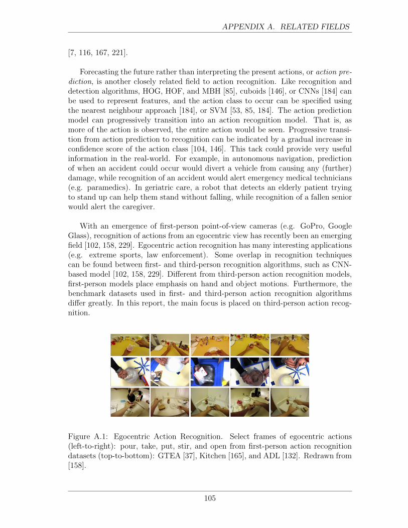
APPENDIX A. RELATED FIELDS
[7, 116, 167, 221].
Forecasting the future rather than interpreting the present actions, or action pre-diction, is another closely related field to action recognition. Like recognition anddetection algorithms, HOG, HOF, and MBH [85], cuboids [146], or CNNs [184] canbe used to represent features, and the action class to occur can be specified usingthe nearest neighbour approach [184], or SVM [53, 85, 184]. The action predictionmodel can progressively transition into an action recognition model. That is, asmore of the action is observed, the entire action would be seen. Progressive transi-tion from action prediction to recognition can be indicated by a gradual increase inconfidence score of the action class [104, 146]. This tack could provide very usefulinformation in the real-world. For example, in autonomous navigation, predictionof when an accident could occur would divert a vehicle from causing any (further)damage, while recognition of an accident would alert emergency medical technicians(e.g. paramedics). In geriatric care, a robot that detects an elderly patient tryingto stand up can help them stand without falling, while recognition of a fallen seniorwould alert the caregiver.
With an emergence of first-person point-of-view cameras (e.g. GoPro, GoogleGlass), recognition of actions from an egocentric view has recently been an emergingfield [102, 158, 229]. Egocentric action recognition has many interesting applications(e.g. extreme sports, law enforcement). Some overlap in recognition techniquescan be found between first- and third-person recognition algorithms, such as CNN-based model [102, 158, 229]. Different from third-person action recognition models,first-person models place emphasis on hand and object motions. Furthermore, thebenchmark datasets used in first- and third-person action recognition algorithmsdiffer greatly. In this report, the main focus is placed on third-person action recog-nition.
Figure A.1: Egocentric Action Recognition. Select frames of egocentric actions(left-to-right): pour, take, put, stir, and open from first-person action recognitiondatasets (top-to-bottom): GTEA [37], Kitchen [165], and ADL [132]. Redrawn from[158].
105

APPENDIX A. RELATED FIELDS
Activity recognition [56] is another closely related active field of research. Activityrecognition in itself is a vast field as it can be broken down into single person activity,group activity, and team activity as in sports [59]. As actions are basic componentsthat piece together to yield an activity, collectively recognizing primitive actions canprovide strong indication of the activity that is occurring in a video. Thus, actionrecognition and detection remains a fundamental problem for its related recognitionand classification tasks.
106
References
[1] M.A.R. Ahad, J. Tan, H. Kim, and S. Ishikawa. Action Dataset - A Survey.In SICE Annual Conference, pages 1650–1655, 2011.
[2] M. Ahmad and S.W. Lee. Human Action Recognition using Shape and CLG-motion flow from Multi-view Image Sequences. The Journal of Pattern Recog-nition Society, 41(7):2237–2252, 2008.
[3] S. Ali and M. Shah. Human Action Recognition in Videos Using KinematicFeatures and Multiple Instance Learning. IEEE Transactions on Pattern Anal-ysis and Machine Intelligence (PAMI), 32(2):288–303, 2010.
[4] R. Arandjelovic and A. Zisserman. All about VLAD. In IEEE Conference onComputer Vision and Pattern Recognition (CVPR), pages 1578–1585, 2013.
[5] M. Baccouche, F. Mamalet, C. Wolf, C. Garcia, and A. Baskurt. SequentialDeep Learning for Human Action Recognition. In Human Behavior Under-standing, pages 29–39, 2011.
[6] N. Ballas, Y. Yang, Z.Z. Lan, B. Delezoide, F. Preteux, and A. Hauptmann.Space-Time Robust Video Representation for Action Recognition. In IEEE In-ternational Conference on Computer Vision (ICCV), pages 2704–2711, 2013.
[7] A. Basharat, A. Gritai, and M. Shah. Learning Object Motion Patterns forAnomaly Detection and Improved Object Detection. In IEEE Conference onComputer Vision and Pattern Recognition (CVPR), pages 1–8, 2008.
[8] D. Batra, T. Chen, and R. Sukthankar. Space-Time Shapelets for ActionRecognition. In IEEE Workshop on Motion and Video Computing (WMVC),pages 1–6, 2008.
[9] H. Bay, T. Tuytelaars, and L. Van Gool. SURF: Speeded Up Robust Features.In European Conference on Computer Vision (ECCV), pages 404–417, 2006.
[10] I. Biederman. Human Image Understanding: Recent Research and a Theory.Computer Vision, Graphics, and Image Processing, 32(1):29–73, 1985.
[11] H. Bilen, B. Fernando, E. Gavves, A. Vedaldi, and S. Gould. Dynamic ImageNetworks for Action Recognition. In IEEE Conference on Computer Visionand Pattern Recognition (CVPR), 2016.
107

REFERENCES REFERENCES
[12] J.A. Bilmes. Dynamic Bayesian Multinets. In Uncertainty in Artificial Intel-ligence, 2000.
[13] C.M. Bishop. Pattern Recognition and Machine Learning. Springer, 2006.
[14] M. Blank, L. Gorelick, E. Shechtman, M. Irani, and R. Basri. Actions asSpace-Time Shapes. In IEEE International Conference on Computer Vision(ICCV), pages 1395–1402, 2005.
[15] D.M. Blei, A.Y. Ng, and M.I. Jordan. Latent Dirichlet Allocation. Journal ofMachine Learning Research (JMLR), 3:993–1022, 2003.
[16] A. Bobick and J. Davis. The Recognition of Human Movement Using TemporalTemplates. IEEE Transactions on Pattern Analysis and Machine Intelligence(PAMI), 23(3):257–267, 2001.
[17] R. Bodor, B. Jackson, and N. Papanikolopoulos. Vision-based Human Track-ing and Activity Recognition. In Mediterranean Conference on Control andAutomation, 2003.
[18] Y.L. Boureau, J. Ponce, and Y. LeCun. A Theoretical Analysis of FeaturePooling in Visual Recognition. In International Conference on Machine Learn-ing (ICML), 2010.
[19] J.C. Caicedo and F.A. Gonzalez. Online Matrix Factorization for MultimodalImage Retrieval. In Progress in Pattern Recognition, Image Analysis, Com-puter Vision, and Applications, pages 340–347, 2012.
[20] L. Cao, Z. Liu, and T.S. Huang. Cross-dataset Action Detection. In IEEE Con-ference on Computer Vision and Pattern Recognition (CVPR), pages 1998–2005, 2010.
[21] J.M. Chalet, E.J. Carmon, and A. Fernandez-Caballero. A Survey of VideoDatasets for Human Action and Activity Recognition. Computer Vision andImage Understanding (CVIU), 117(6):633–659, 2013.
[22] K. Chatfield, V. Lemtexpitsky, A. Vedaldi, and A. Zisserman. The Devil is inthe Details: An Evaluation of Recent Feature Encoding Methods. In BritishMachine Vision Conference (BMVC), pages 76.1–76.12, 2011.
[23] W. Chen, C. Xiong, R. Xu, and J.J. Corso. Actionness Ranking with LatticeConditional Ordinal Random Fields. In IEEE Conference on Computer Visionand Pattern Recognition (CVPR), pages 748–755, 2014.
[24] O. Chomat and J. Crowley. Probabilistic Recognition of Activity Using LocalAppearance. In IEEE Conference on Computer Vision and Pattern Recogni-tion (CVPR), 1999.
108

REFERENCES REFERENCES
[25] N. Dalal and B. Triggs. Histograms of Oriented Gradients for Human De-tection. In IEEE Conference on Computer Vision and Pattern Recognition(CVPR), volume 1, pages 886–893, 2005.
[26] N. Dalal, B. Triggs, and C. Schmid. Human Detection Using Oriented His-tograms of Flow and Appearance. In European Conference on Computer Vi-sion (ECCV), volume 3952, pages 428–441, 2006.
[27] J. Deng, W. Dong, R. Socher, L.J. Li, K. Li, and L. Fei-Fei. ImageNet: ALarge-scale Hierarchical Image Database. In IEEE Conference on ComputerVision and Pattern Recognition (CVPR), 2009.
[28] K. Derpanis, M. Sizintsev, K.J. Cannons, and R.P. Wildes. Action Spot-ting and Recognition Based on a Spatiotemporal Orientation Analysis. IEEETransactions on Pattern Analysis and Machine Intelligence (PAMI), 35(3):1–8, 2013.
[29] P. Dollar, V. Rabaud, G. Cottrell, and S. Belongie. Behavior Recognition viaSparse Spatio-Temporal Features. In Joint IEEE International Workshop onVisual Surveillance and Performance Evaluation of Tracking and Surveillance,pages 65–72, 2005.
[30] J. Donahue, L.A. Hendricks, S. Guadarrama, and M. Rohrbach. Long-termRecurrent Convolutional Networks for Visual Recognition and Description.In IEEE Conference on Computer Vision and Pattern Recognition (CVPR),pages 2625–2634, 2015.
[31] G. Dougherty. Pattern Recognition and Classification. Springer, 2013.
[32] Y. Du, F. Chen, and W. Xu. Human Interaction Representation and Recog-nition Through Motion Decomposition. IEEE Signal Processing Letters,14(12):952–955, 2007.
[33] R.O. Duda, P.E. Hart, and D.G. Stork. Pattern Classification. John Wiley &Sons, 2001.
[34] A.A. Efros, A.C. Berg, G. Mori, and J. Malik. Recognizing Action at a Dis-tance. In IEEE International Conference on Computer Vision (ICCV), pages726 – 733, October 2003.
[35] C. Fanti, L. Zelnik Manor, and P. Perona. Hybrid Models for Human MotionRecognition. In IEEE Conference on Computer Vision and Pattern Recogni-tion (CVPR), pages 1166–1173, 2005.
[36] A. Fathi and G. Mori. Action Recognition by Learning Mid-Level MotionFeatures. In IEEE Conference on Computer Vision and Pattern Recognition(CVPR), 2008.
109

REFERENCES REFERENCES
[37] A. Fathi, X. Ren, and J.M. Rehg. Learning to Recognize Objects in EgocentricActivities. In IEEE Conference on Computer Vision and Pattern Recognition(CVPR), pages 3281–3288, 2011.
[38] C. Feichtenhofer, A. Pinz, and R.P. Wildes. Dynamically Encoded Actionsbased on Spacetime Saliency. In IEEE Conference on Computer Vision andPattern Recognition (CVPR), pages 2755–2764, 2015.
[39] C. Feichtenhofer, A. Pinz, and R.P. Wildes. Dynamic Scene Recognitionwith Complementary Spatiotemporal Features. IEEE Transactions on Pat-tern Analysis and Machine Intelligence (PAMI), pages 1–14, 2016.
[40] C. Feichtenhofer, A. Pinz, and R.P. Wildes. Spatiotemporal Residual Networksfor Video Action Recognition. In Advances in Neural Information ProcessingSystems (NIPS), 2016.
[41] C. Feichtenhofer, A. Pinz, and A. Zisserman. Convolutional Two-Stream Net-work Fusion for Video Action Recognition. In IEEE Conference on ComputerVision and Pattern Recognition (CVPR), pages 1933–1941, 2016.
[42] X. Feng and P. Perona. Human Action Recognition by Sequence of MoveletCodewords. In First International Symposium on 3D Data Processing Visu-alization and Transmission, pages 717–721, 2002.
[43] B. Fernando, P. Anderson, M. Hutter, and S. Gould. Discriminative Hierarchi-cal Rank Pooling for Activity Recognition. In IEEE Conference on ComputerVision and Pattern Recognition (CVPR), pages 1924–1932, 2016.
[44] K. Fukushima. Neocognitron: A self-organizing neural network model for amechanism of pattern recognition. Biological Cybernetics, 36(4):193–202, 1980.
[45] K. Gimpel. Modeling Topics. Technical report, Carnegie Mellon University,2008.
[46] G. Gkioxari and J. Malik. Finding Action Tubes. In IEEE Conference onComputer Vision and Pattern Recognition (CVPR), pages 759–768, 2015.
[47] M.A. Goodale and A.D. Milner. Separate Visual Pathways for Perception andAction. Trends in Neurosciences, 15(1):20–25, 1992.
[48] A. Gorban, H. Idrees, Y.G. Jiang, A. Roshan Zamir, I. Laptev, M. Shah,and R. Sukthankar. THUMOS Challenge: Action Recognition with a LargeNumber of Classes. http://www.thumos.info/, 2015.
[49] J.M. Gryn, R.P. Wildes, and J.K. Tsotsos. Detecting Motion Patterns viaDirection Maps with Application to Surveillance. Computer Vision and ImageUnderstanding (CVIU), 113(2):291–307, 2009.
[50] M. Hahn, L. Kruger, and C. Wohler. 3D Action Recognition and Long-TermPrediction of Human Motion. In Computer Vision Systems, pages 23–32, 2008.
110

REFERENCES REFERENCES
[51] F.C. Heilbron, V. Escorcia, B. Ghanem, and J.C. Niebles. ActivityNet: ALarge-Scale Video Benchmark for Human Activity Understanding. In IEEEConference on Computer Vision and Pattern Recognition (CVPR), pages 961–970, 2015.
[52] F.C. Heilbron, J.C. Niebles, and B. Ghanem. Fast Temporal Activity Pro-posals for Efficient Detection of Human Actions in Untrimmed Videos. InIEEE Conference on Computer Vision and Pattern Recognition (CVPR),pages 1914–1923, 2016.
[53] M. Hoai and F. de la Torre. Max-Margin Early Event Detectors. InternationalJournal of Computer Vision (IJCV), 107(2):191–202, 2014.
[54] T. Hofmann. Probabilistic Latent Semantic Indexing. In Annual Interna-tional ACM SIGIR Conference on Research and Development in InformationRetrieval, pages 50–57, 1999.
[55] M.K. Hu. Visual Pattern Recognition by Moment Invariants. IRE Transac-tions on Information Theory, 8(2):179–187, 1962.
[56] W. Hu, T. Tan, L. Wang, and S. Maybank. A Survey on Visual Surveillance ofObject Motion and Behaviors. In IEEE Transactions on Systems, Man, andCybernetics, pages 334–352, 2006.
[57] G.B. Huang, H. Zhou, X. Ding, and R. Zhang. Extreme Learning Machine forRegression and Multiclass Classification. In IEEE Transactions on Systems,Man, and Cybernetics, volume 42, pages 513–529, 2012.
[58] Y. Huang, K. Huang, Y. Yu, and T. Tan. Salient Coding for Image Classi-fication. In IEEE Conference on Computer Vision and Pattern Recognition(CVPR), pages 1753–1760, 2011.
[59] M.S. Ibrahim, S. Muralidharan, Z. Deng, A. Vahdat, and G. Mori. A Hierar-chical Deep Temporal Model for Group Activity Recognition. In IEEE Confer-ence on Computer Vision and Pattern Recognition (CVPR), pages 1971–1980,2016.
[60] N. Ikizler and P. Duygulu. Histogram of oriented rectangles: A new pose de-scriptor for human action recognition. Image Vision Computing, 27(10):1515–1526, 2009.
[61] N. Ikizler and D.A. Forsyth. Searching for Complex Human Activities withNo Visual Examples. International Journal of Computer Vision (IJCV),80(3):337–357, 2008.
[62] T.S. Jaakkola and D. Haussler. Exploiting Generative Models in Discrim-inative Classifiers. In Advances in Neural Information Processing Systems(NIPS), pages 487–493, 1998.
111

REFERENCES REFERENCES
[63] M. Jain, H. Jegou, and P. Bouthemy. Better Exploiting Motion for BetterAction Recognition. In IEEE Conference on Computer Vision and PatternRecognition (CVPR), pages 2555–2562, 2013.
[64] M. Jain, J. van Gemert, H. Jegou, P. Bouthemy, and C.G.M. Snoek. ActionLocalization with Tubelets from Motion. In IEEE Conference on ComputerVision and Pattern Recognition (CVPR), pages 740–747, 2014.
[65] H. Jegou, M. Douze, C. Schmid, and P. Perez. Aggregating Local Descriptorsinto a Compact Image Representation. In IEEE Conference on ComputerVision and Pattern Recognition (CVPR), pages 3304–3311, 2010.
[66] H. Jhuang, J. Gall, S. Zuffi, C. Schmid, and M.J. Black. Towards Under-standing Action Recognition. In IEEE International Conference on ComputerVision (ICCV), pages 3192–3199, 2013.
[67] H. Jhuang, T. Serre, L. Wolf, and T. Poggio. A Biologically Inspired System forAction Recognition. In IEEE International Conference on Computer Vision(ICCV), 2007.
[68] S. Ji, W. Xu, M. Yang, and K. Yu. 3D Convolutional Neural Networks forHuman Action Recognition. IEEE Transactions on Pattern Analysis and Ma-chine Intelligence (PAMI), 35(1):221–231, 2013.
[69] Y.G. Jiang, Q. Dai, X. Xue, W. Liu, and C.W. Ngo. Trajectory-Based Model-ing of Human Actions with Motion Reference Points. In European Conferenceon Computer Vision (ECCV), volume 7576, pages 425–438, 2012.
[70] Y.G. Jiang, J. Liu, A. Roshan Zamir, I. Laptev, M. Piccardi, M. Shah, andR. Sukthankar. THUMOS Challenge: Action Recognition with a Large Num-ber of Classes. http://crcv.ucf.edu/ICCV13-Action-Workshop/, 2013.
[71] Y.G. Jiang, J. Liu, A. Roshan Zamir, G. Toderici, I. Laptev, M. Shah, andR. Sukthankar. THUMOS Challenge: Action Recognition with a Large Num-ber of Classes. http://crcv.ucf.edu/THUMOS14/, 2014.
[72] S.X. Ju, M.J. Black, and Y. Yacoob. Cardboard People: A ParameterizedModel of Articulated Image Motion. In Proceedings of the Second InternationalConference on Automatic Face and Gesture Recognition, pages 38–44, 1996.
[73] A. Karpathy, G. Toderici, S. Shetty, T. Leung, R. Sukthankar, and L. Fei-Fei.Large-scale Video Classification with Convolutional Neural Networks. In IEEEConference on Computer Vision and Pattern Recognition (CVPR), pages 1725– 1732, 2014.
[74] S.R. Ke, H.L.U. Thuc, Y.J. Lee, J.N Hwang, J.H. Yoo, and K.H. Choi. AReview on Video-Based Human Activity Recognition. Activity Detection andNovel Sensing Technologies, 2(2):88–131, 2013.
112
REFERENCES REFERENCES
[75] Y. Ke, R. Sukthankar, and M. Hebert. Efficient Visual Event Detection usingVolumetric Features. In IEEE International Conference on Computer Vision(ICCV), pages 166–173, 2005.
[76] Y. Ke, R. Sukthankar, and M. Hebert. Event Detection in Crowded Videos.In IEEE International Conference on Computer Vision (ICCV), pages 1–8,2007.
[77] T. Kim and R. Cupola. Canonical Correlation Analysis of Video Volume Ten-sors for Action Categorization and Detection. IEEE Transactions on PatternAnalysis and Machine Intelligence (PAMI), 31:1415–1428, 2009.
[78] A. Klaser, M. Marszalek, and C. Schmid. A Spatio-Temporal Descriptor Basedon 3D-Gradients. In British Machine Vision Conference (BMVC), 2008.
[79] O. Kliper-Gross, Y. Gurovich, T. Hassner, and L. Wolf. Motion InterchangePatterns for Action Recognition in Unconstrained Videos. In European Con-ference on Computer Vision (ECCV), 2012.
[80] J.J. Koenderink and A.J. Van Doom. The Structure of Locally OrderlessImages. International Journal of Computer Vision (IJCV), 31(2):159–168,1999.
[81] B. Kolman and D.R. Hill. Elementary Linear Algebra with Applications. Pear-son Education Inc., ninth edition edition, 2008.
[82] A. Kovashka and K. Grauman. Learning a Hierarchy of Discriminative Space-Time Neighborhood Features for Human Action Recognition. In IEEE Confer-ence on Computer Vision and Pattern Recognition (CVPR), pages 2046–2053,2010.
[83] H. Kuehne, H. Jhuang, E. Garrote, T. Poggio, and T. Serre. HMDB: ALarge Video Database for Human Motion Recognition. In IEEE InternationalConference on Computer Vision (ICCV), pages 2556–2563, 2011.
[84] J. Lafferty, A. McCallum, and F. Pereira. Conditional Random Fields: Prob-abilistic Models for Segmenting and Labeling Sequence Data. In InternationalConference on Machine Learning (ICML), pages 282–289, 2001.
[85] T. Lan, T.C. Chen, and S. Savarese. A Hierarchical Representation for FutureAction Prediction. In European Conference on Computer Vision (ECCV),pages 689–704, 2014.
[86] T. Lan, Y. Wang, and G. Mori. Discriminative Figure-centric Models for JointAction Localization and Recognition. In IEEE International Conference onComputer Vision (ICCV), pages 2003–2010, 2011.
[87] I. Laptev. On Space-Time Interest Points. International Journal of ComputerVision (IJCV), 64(2):107–123, 2005.
113

REFERENCES REFERENCES
[88] I. Laptev, M. Marszalek, C. Schmid, and B. Rozenfeld. Learning RealisticHuman Actions from Movies. In IEEE Conference on Computer Vision andPattern Recognition (CVPR), 2008.
[89] I. Laptev and P. Perez. Retrieving Actions in Movies. In IEEE InternationalConference on Computer Vision (ICCV), pages 1–8, 2007.
[90] B. Laxton, L. Lim, and D. Kriegman. Leveraging Temporal, Contextual andOrdering Constraints for Recognizing Complex Activities in Video. In IEEEConference on Computer Vision and Pattern Recognition (CVPR), pages 1–8,2007.
[91] S. Lazebnik, C. Schmid, and J. Ponce. Beyond Bags of Features: Spatial Pyra-mid Matching for Recognizing Natural Scene Categories. In IEEE Conferenceon Computer Vision and Pattern Recognition (CVPR), pages 2169–2178, 2006.
[92] Q.V. Le, W.Y. Zou, S.Y. Yeung, and A.Y. Ng. Learning Hierarchical InvariantSpatio-temporal Features for Action Recognition with Independent SubspaceAnalysis. In IEEE Conference on Computer Vision and Pattern Recognition(CVPR), pages 3361–3368, 2011.
[93] Y. LeCun, L. Bottou, Y. Bengio, and P. Haffner. Gradient-based LearningApplied to Document Recognition. In Proceedings of the IEEE, volume 86,1998.
[94] Z. Lin, Z. Jiang, and L. Davis. Recognizing Actions by Shape-Motion Proto-type Trees. In IEEE International Conference on Computer Vision (ICCV),pages 444–451, 2009.
[95] H. Liu, R. Feris, and M.T. Sun. Visual Analysis of Humans, chapter 20- Benchmarking Datasets for Human Activity Recognition, pages 411–427.Springer, 2011.
[96] J. Liu, J. Luo, and M. Shah. Recognizing Realistic Actions from Videos “inthe wild”. In IEEE Conference on Computer Vision and Pattern Recognition(CVPR), 2009.
[97] L. Liu, L. Wang, and X. Liu. In Defense of Soft-Assignment Coding. InIEEE International Conference on Computer Vision (ICCV), pages 2486–2493, 2011.
[98] D. Lowe. Distinctive Image Features from Scale-Invariant Keypoints. Inter-national Journal of Computer Vision (IJCV), 60(2):91–110, 2004.
[99] W.L. Lu and J.J. Little. Simultaneous Tracking and Action Recognition usingthe PCA-HOG Descriptor. In Canadian Conference on Computer and RobotVision (CRV), pages 1–6, 2006.
114

REFERENCES REFERENCES
[100] Y. Luo, T.D. Wu, and J.N. Hwang. Object-based Analysis and Interpretationof Human Motion in Sports Video Sequences by Dynamic Bayesian Networks.Computer Vision and Image Understanding (CVIU), 92(2-3):196–216, 2003.
[101] F. Lv and R. Nevatia. Single View Human Action Recognition using KeyPose Matching and Viterbi Path Searching. In IEEE Conference on ComputerVision and Pattern Recognition (CVPR), pages 1–8, 2007.
[102] M. Ma, H. Fan, and K.M. Kitani. Going Deeper into First-Person ActivityRecognition. In IEEE Conference on Computer Vision and Pattern Recogni-tion (CVPR), pages 1894–1903, 2016.
[103] S. Ma, S. Sclaroff, J. Zhang, and N. Ikizler-cinbis. Action Recognition andLocalization by Hierarchical Space-Time Segments. In IEEE InternationalConference on Computer Vision (ICCV), 2013.
[104] S. Ma, L. Sigal, and S. Sclaroff. Learning Activity Progression in LSTMs forActivity Detection and Early Detection. In IEEE Conference on ComputerVision and Pattern Recognition (CVPR), pages 1942–1950, 2016.
[105] B. Mahasseni and S. Todorovic. Regularizing Long Short Term Memory with3D Human-Skeleton Sequences for Action Recognition. In IEEE Conferenceon Computer Vision and Pattern Recognition (CVPR), pages 3054–3062, 2016.
[106] M. Marszalek, I. Laptev, and C. Schmid. Hollywood2: Human Actions andScenes Dataset. http://www.di.ens.fr/~laptev/actions/hollywood2/.
[107] M. Marszalek, I. Laptev, and C. Schmid. Actions in Context. In IEEE Confer-ence on Computer Vision and Pattern Recognition (CVPR), pages 2929–2936,2009.
[108] T. Masada, S. Kiyasu, and S. Miyahara. Comparing LDA with pLSI as aDimensionality Reduction Method in Document Clustering. In Conference onLarge-Scale Knowledge Resources, pages 13–26, 2008.
[109] J. Matas, O. Chum, M. Urban, and T. Pajdla. Robust Wide-Baseline Stereofrom Maximally Stable Extremal Regions. In British Machine Vision Confer-ence (BMVC), pages 384–396, 2004.
[110] M.A. Mendoza and N.P. de la Blanca. Applying Space State Models in Hu-man Action Recognition: A Comparative Study. In Articulated Motion andDeformable Objects (AMDO), pages 53–62, 2008.
[111] K. Mikolajczyk and C. Schmid. Indexing based on Scale Invariant InterestPoints. In IEEE International Conference on Computer Vision (ICCV), 2001.
[112] K. Mikolajczyk and C. Schmid. Scale and Affine Invariant Interest PointDetectors. International Journal of Computer Vision (IJCV), 60(1):63–86,2004.
115

REFERENCES REFERENCES
[113] K. Mikolajczyk and C. Schmid. A Performance Evaluation of Local De-scriptors. IEEE Transactions on Pattern Analysis and Machine Intelligence(PAMI), 27(10):1615–1630, 2005.
[114] K. Mikolajczyk and H. Uemura. Action Recognition with Motion-AppearanceVocabulary Forest. In IEEE Computer Vision and Pattern Recognition(CVPR), 2008.
[115] C. Moler. The World’s Largest Matrix Computation. Technical articles andnewsletters, MathWorks, 2002.
[116] R.J. Morris and D.C. Hogg. Statistical Models of Object Interaction. Inter-national Journal of Computer Vision (IJCV), 37(2):209–215, 2000.
[117] K. Murphy. Dynamic Bayesian Networks: Representation, Inference andLearning. PhD thesis, University of California, Berkeley, 2002.
[118] J.Y.H. Ng, M. Hausknecht, S. Vijayanarasimhan, O. Vinyals, R. Monga, andG. Toderici. Beyond Short Snippets: Deep Networks for Video Classification.In IEEE Conference on Computer Vision and Pattern Recognition (CVPR),pages 4694–4702, 2015.
[119] D.H. Nga and K. Yanai. A Spatio-Temporal Feature based on Triangula-tion of Dense SURF. In IEEE International Conference on Computer VisionWorkshops (ICCVW), pages 420–427, 2013.
[120] B. Ni, X. Yang, and S. Gao. Progressively Parsing Interactional Objects forFine Grained Action Detection. In IEEE Conference on Computer Vision andPattern Recognition (CVPR), pages 1020–1028, 2016.
[121] J.C. Niebles, C.W. Chen, and L. Fei-Fei. Modeling Temporal Structure ofDecomposable Motion Segments for Activity Classification. In European Con-ference on Computer Vision (ECCV), volume 2, pages 392–405, 2010.
[122] J.C. Niebles, H. Wang, and L. Fei-Fei. Unsupervised Learning of HumanAction Categories Using Spatial-Temporal Words. International Journal ofComputer Vision (IJCV), 79:299–318, 2008.
[123] H. Ning, T. Han, D. Walther, M. Liu, and T. Huang. Hierarchical Space-TimeModel Enabling Efficient Search for Human Actions. In IEEE Transactions inCircuits and Systems for Video Technology, volume 19, pages 808–820, 2006.
[124] T. Ogata, W. Christmas, J. Kittler, and S. Ishikawa. Improving Human Ac-tivity Detection by Combining Multi-dimensional Motion Descriptors withBoosting. In International Conference on Pattern Recognition (ICPR), vol-ume 1, pages 295–298, 2006.
[125] A. Oikonomopoulos, I. Patras, and M. Pantic. Spatiotemporal Salient Pointsfor Visual Recognition of Human Actions. In IEEE Transactions on Systems,Man, and Cybernetics - Part B: Cybernetics, volume 36, pages 710–719, 2006.
116

REFERENCES REFERENCES
[126] D. Oneata, J. Revaud, J. Verbeek, and C. Schmid. Spatio-temporal ObjectDetection Proposals. In European Conference on Computer Vision (ECCV),pages 737–752, 2014.
[127] D. Oneata, J. Verbeek, and C. Schmid. Action and Event Recognition withFisher Vectors on a Compact Feature Set. In IEEE International Conferenceon Computer Vision (ICCV), pages 1817–1824, 2013.
[128] D. Oneata, J. Verbeek, and C. Schmid. The LEAR submission at THUMOS2014. In THUMOS Challenge: Action Recognition with a Large Number ofClasses, 2014.
[129] L. Page, S. Brin, R. Motwani, and T. Winograd. The PageRank CitationRanking: Bringing Order to the Web. Technical Report 422, Stanford Uni-versity, 1999.
[130] X. Peng, L. Wang, X. Wang, and Y. Qiao. Bag of Visual Words and FusionMethods for Action Recognition: Comprehensive Study and Good Practice.Computer Vision and Image Understanding (CVIU), 150:109–125, 2016.
[131] F. Perronnin, J. Sanchez, and Thomas Mensink. Improving the Fisher Kernelfor Large-Scale Image Classification. In European Conference on ComputerVision (ECCV), pages 143–156, 2010.
[132] H. Pirsiavash and D. Ramanan. Detecting Activities of Daily Living in First-person Camera Views. In IEEE Conference on Computer Vision and PatternRecognition (CVPR), pages 2847–2854, 2012.
[133] R. Poppe. A Survey on Vision-based Human Action Recognition. Image andVision Computing, 28(6):976–990, 2010.
[134] J. Puzicha, T. Hofmann, and J.M. Buhmann. Non-parametric Similarity Mea-sures for Unsupervised Texture Segmentation and Image Retrieval. In IEEEConference on Computer Vision and Pattern Recognition (CVPR), pages 267–272, 1997.
[135] D. Ramanan and D.A. Forsyth. Automatic Annotation of Everyday Move-ments. In Advances in Neural Information Processing Systems (NIPS), 2003.
[136] C. Rao, A. Yilmaz, and M. Shah. View-Invariant Representation and Recogni-tion of Actions. International Journal of Computer Vision (IJCV), 50(2):203–226, 2002.
[137] K. Rapantzikos, Y. Avrithis, and S. Kollias. Dense Saliency-Based Spatiotem-poral Feature Points for Action Recognition. In IEEE Conference on ComputerVision and Pattern Recognition (CVPR), 2009.
[138] K.K. Reddy and M. Shah. UCF50 - Action Recognition Data Set. http:
//crcv.ucf.edu/data/UCF50.php.
117

REFERENCES REFERENCES
[139] K.K. Reddy and M. Shah. Recognizing 50 Human Action Categories of WebVideos. Machine Vision and Applications Journal, 24(5):971–981, 2012.
[140] M. Rodriguez, J. Ahmed, and M. Shah. Action MACH: A Spatio-temporalMaximum Average Correlation Height Filter for Action Recognition. In IEEEConference on Computer Vision and Pattern Recognition (CVPR), 2008.
[141] M. Rohrbach, S. Amin, M. Andriluka, and B. Schiele. A Database for FineGrained Activity Detection of Cooking Activities. In IEEE Conference onComputer Vision and Pattern Recognition (CVPR), pages 1194–1201, 2012.
[142] M. Rohrbach, A. Rohrbach, M. Regneri, S. Amin, M. Andriluka, M. Pinkal,and B. Schiele. Recognizing Fine-Grained and Composite Activities UsingHand-Centric Features and Script Data. International Journal of ComputerVision (IJCV), 119(3):346–373, 2015.
[143] Y. Rubner, C. Tomasi, and L.J. Guibas. A Metric for Distributions with Appli-cations to Image Databases. In IEEE International Conference on ComputerVision (ICCV), pages 59–66, 1998.
[144] Y. Rubner, C. Tomasi, and L.J. Guibas. The Earth Mover’s Distance as aMetric for Image Retrieval. International Journal of Computer Vision (IJCV),40(2):99–121, 2000.
[145] S. Russell and P. Norvig. Artificial Intelligence: A Modern Approach. PrenticeHall, third edition edition, 2010.
[146] M.S. Ryoo. Human Activity Prediction: Early Recognition of Ongoing Activ-ities from Streaming Videos. In IEEE International Conference on ComputerVision (ICCV), pages 1036–1043, 2011.
[147] K. Schindler and L. van Gool. Action Snippets: How many frames doeshuman action recognition require? In IEEE Conference on Computer Visionand Pattern Recognition (CVPR), pages 1–8, 2008.
[148] C. Schuldt, I. Laptev, and B. Caputo. Recognizing Human Action: A Lo-cal SVM Approach. In IEEE Conference on Computer Vision and PatternRecognition (CVPR), pages 32–36, 2004.
[149] P. Scovanner, S. Ali, and M. Shah. A 3-Dimensional SIFT Descriptor and ItsApplications to Action Recognition. In Proceedings of the 15th ACM Interna-tional Conference on Multimedia, pages 357–360, 2007.
[150] T. Serre, L. Wolf, S. Bileschi, M. Riesenhuber, and T. Poggio. Robust ObjectRecognition with Cortex-like Mechanisms. IEEE Transactions on PatternAnalysis and Machine Intelligence (PAMI), 29(3):411–426, 2007.
[151] A.H. Shabani, D.A. Clausi, and J.S. Zelek. Salient Feature Detectors forHuman Action Recognition. In Ninth Conference on Computer and RobotVision (CRV), pages 468–475, 2012.
118

REFERENCES REFERENCES
[152] E. Shechtman and M. Irani. Space-Time Behavior-Based Correlation - OR -How to Tell If Two Underlying Motion Fields are Similar without ComputingThem? IEEE Transactions on Pattern Analysis and Machine Intelligence(PAMI), 29:2045–2056, 2007.
[153] F. Shi, E.M. Petriu, and A. Cordeiro. Human Action Recognition from Lo-cal Part Model. In IEEE International Workshop on Haptic Audio VisualEnvironments and Games (HAVE), 2011.
[154] J. Shi and C. Tomasi. Good Features to Track. In IEEE Conference onComputer Vision and Pattern Recognition (CVPR), pages 593–600, 1994.
[155] Z. Shou, D. Wang, and S.F. Chang. Temporal Action Localization inUntrimmed Videos via Multi-stage CNNs. In IEEE Conference on ComputerVision and Pattern Recognition (CVPR), pages 1049–1058, 2016.
[156] K. Simonyan and A. Zisserman. Two-Stream Convolutional Networks for Ac-tion Recognition in Videos. In Advances in Neural Information ProcessingSystems (NIPS), 2014.
[157] B. Singh, T.K. Marks, O. Tuzel M. Jones, and M. Shao. A Multi-StreamBi-Direction recurrent Neural Network for Fine-Grained Action Detection.In IEEE Conference on Computer Vision and Pattern Recognition (CVPR),pages 1961–1970, 2016.
[158] S. Singh, C. Arora, and C.V. Jawahar. First Person Action Recognition UsingDeep Learned Descriptors. In IEEE Conference on Computer Vision andPattern Recognition (CVPR), pages 2620–2628, 2016.
[159] J. Sivic and A. Zisserman. Efficient Visual Search of Videos Cast as TextRetrieval. IEEE Transactions on Pattern Analysis and Machine Intelligence(PAMI), 31:591–606, 2009.
[160] C. Sminchisescu, A. Kanaujia, L. Li, and D. Metaxas. Conditional Models forContextual Human Motion Recognition. In IEEE International Conferenceon Computer Vision (ICCV), pages 1808–1815, 2005.
[161] C. Snoek, B. Ghanem, J.C. Niebles, F.C. Heilbron, W. Barrios, V. Escorcia,and P. Mettes. ActivityNet: A Large-Scale Activity Recognition Challenge.http://activity-net.org/challenges/2016/index.html, 2016.
[162] K. Soomro and A.R. Zamir. Computer Vision in Sports, chapter 9 - ActionRecognition in Realistic Sports Videos, pages 181–208. Springer, 2014.
[163] K. Soomro, A.R. Zamir, and M. Shah. UCF101: A Dataset of 101 HumanActions Classes from Videos in the Wild. Technical Report CRCV-TR-12-01,University of Central Florida, 2012.
119

REFERENCES REFERENCES
[164] R. Souvenir and J. Babbs. Learning the Viewpoint Manifold for Action Recog-nition. In IEEE Conference on Computer Vision and Pattern Recognition(CVPR), 2008.
[165] E.H. Spriggs, F. de la Torre, and M. Hebert. Temporal Segmentation andActivity Classification from First-Person Sensing. In IEEE Conference onComputer Vision and Pattern Recognition Workshops (CVPRW), pages 17–24, 2009.
[166] J. T. Springenberg, A. Dosovitskiy, T. Brox, and M. Riedmiller. Strivingfor Simplicity: The All Convolutional Net. In International Conference onLearning Representation (ICLR), 2015.
[167] C. Stauffer and E.L. Grimson. Learning Patterns of Activity Using Real-TimeTracking. IEEE Transactions on Pattern Analysis and Machine Intelligence(PAMI), 22:747–757, 2000.
[168] W. Sultani and I. Saleemi. Human Action Recognition across Datasets byForeground-weighted Histogram Decomposition. In IEEE Conference on Com-puter Vision and Pattern Recognition (CVPR), pages 764–771, 2014.
[169] W. Sultani and M. Shah. What if we do not have multiple videos of the sameaction? - Video Action Localization Using Web Images. In IEEE Conferenceon Computer Vision and Pattern Recognition (CVPR), pages 1077–1085, 2016.
[170] J. Sun, X. Wu, S. Yan, L. Cheong, T. Chua, and J. Li. Hierarchical Spatio-Temporal Context Modeling for Action Recognition. In IEEE Conference onComputer Vision and Pattern Recognition (CVPR), 2009.
[171] C. Sutton and A. McCallum. An Introduction to Conditional Random Fields.Foundations and Trends in Machine Learning, 4(4):267–373, 2012.
[172] M.J. Swain and D.H. Ballard. Color Indexing. International Journal of Com-puter Vision (IJCV), 7(1):11–32, 1991.
[173] Y. Tian, R. Sukthankar, and M. Shah. Spatiotemporal Deformable Part Mod-els for Action Detection. In IEEE Conference on Computer Vision and PatternRecognition (CVPR), 2013.
[174] E. Di Tomaso and J.F. Baldwin. An Approach to Hybrid Probabilistic Models.International Journal of Approximate Reasoning, 47(2):202–218, 2008.
[175] D. Tran, L. Bourdev, R. Fergus, L. Torresani, and M. Paluri. Learning Spa-tiotemporal Features with 3D Convolutional Networks. In IEEE InternationalConference on Computer Vision (ICCV), pages 4489–4497, 2015.
[176] J.A. Tropp and A.C. Gilbert. Signal Recovery from Random Measurements viaOrthogonal Matching Pursuit. In IEEE Transactions on Information Theory,volume 53, pages 4655–4666, 2007.
120

REFERENCES REFERENCES
[177] H. Uemura, S. Ishikawa, and K. Mikolajczyk. Feature Tracking and MotionCompensation for Action Recognition. In British Machine Vision Conference(BMVC), 2008.
[178] M.M. Ullah, S.N. Parizi, and I. Laptev. Improving Bag of Features ActionRecognition with Non-Local Cues. In British Machine Vision Conference(BMVC), pages 95.1–95.11, 2010.
[179] L. van der Maaten, E. Postma, and J. van den Herik. Dimensionality Re-duction: A Comparative Review. Technical Report 005, Tilburg University,2009.
[180] J.C. van Gemert, M. Jain, E. Gati, and C.G.M. Snoek. APT: Action Localiza-tion Proposals from Dense Trajectories. In British Machine Vision Conference(BMVC), pages 1–12, 2015.
[181] G. Varol and A.A. Salah. Extreme Learning Machine for Large-Scale ActionRecognition. In THUMOS Challenge: Action Recognition with a Large Numberof Classes, 2014.
[182] A. Veeraraghavan, R. Chellappa, and A.K. Roy-Chowdhury. The FunctionSpace of an Activity. In IEEE Conference on Computer Vision and PatternRecognition (CVPR), pages 959–968, 2006.
[183] E. Vig, M. Dorr, and D. Cox. Space-Variant Descriptor Sampling for ActionRecognition Based on Saliency and Eye Movements. In European Conferenceon Computer Vision (ECCV), pages 84–97, 2012.
[184] C. Vondrick, H. Pirsiavash, and A. Torralba. Anticipating Visual Represen-tations from Unlabeled Video. In IEEE Conference on Computer Vision andPattern Recognition (CVPR), pages 98–106, 2016.
[185] T.H. Vu, C. Olsson, I. Laptev, A. Oliva, and J. Sivic. Predicting Actions fromStatic Scenes. In European Conference on Computer Vision (ECCV), pages421–436, 2014.
[186] H. Wang, A. Klaser, C. Schmid, and C.L. Liu. Action Recognition by DenseTrajectories. In IEEE Conference on Computer Vision and Pattern Recogni-tion (CVPR), pages 3169–3176, 2011.
[187] H. Wang, A. Klaser, C. Schmid, and C.L. Liu. Dense Trajectories and Mo-tion Boundary Descriptors for Action Recognition. International Journal ofComputer Vision (IJCV), 103:60–79, 2013.
[188] H. Wang and C. Schmid. Action Recognition with Improved Trajectories. InIEEE International Conference on Computer Vision (ICCV), 2013.
[189] H. Wang and C. Schmid. LEAR-INRIA Submission for the THUMOS Work-shop. In THUMOS Challenge: Action Recognition with a Large Number ofClasses, 2013.
121

REFERENCES REFERENCES
[190] H. Wang, M. Ullah, A. Klaser, I. Laptev, and C. Schmid. Evaluation of LocalSpatio-Temporal Features for Action Recognition. In British Machine VisionConference (BMVC), 2009.
[191] J. Wang, P. Liu, M.F.H. She, A. Kouzani, and S. Nahavandi. SupervisedLearning Probabilistic Latent Semantic Analysis for Human Motion Analysis.Neurocomputing, 100:134–143, 2013.
[192] J. Wang, J. Yang, K. Yu, F. Lv, T. Huang, and Y. Gong. Locality-constrainedLinear Coding for Image Classification. In IEEE Conference on ComputerVision and Pattern Recognition (CVPR), pages 3360–3367, 2010.
[193] L. Wang, Y. Qiao, and X. Tang. Action Recognition with Trajectory-PooledDeep Convolutional Descriptors. In IEEE Conference on Computer Visionand Pattern Recognition (CVPR), pages 4305–4314, 2015.
[194] L. Wang, Z. Wang, Y. Xiong, and Y. Qiao. CUHK&SIAT Submission forTHUMOS15 Action Recognition Challenge. In THUMOS Challenge: ActionRecognition with a Large Number of Classes, 2015.
[195] X. Wang, A. Farhadi, and A. Gupta. Actions ∼ Transformations. In IEEEConference on Computer Vision and Pattern Recognition (CVPR), pages2658–2667, 2016.
[196] X. Wang, L.M. Wang, and Y. Qiao. A Comparative Study of Encoding,Pooling and Normalization Methods for Action Recognition. In 11th AsianConference on Computer Vision (ACCV), pages 572–585, 2013.
[197] Y. Wang and M. Hoai. Improving Human Action Recognition by Non-actionClassification. In IEEE Conference on Computer Vision and Pattern Recog-nition (CVPR), pages 2698–2707, 2016.
[198] Y. Wang, K. Huang, and T. Tan. Human Activity Recognition Based onR Transform. In IEEE Computer Vision and Pattern Recognition (CVPR),2007.
[199] Y. Wang and G. Mori. Human Action Recognition by Semilatent Topic Mod-els. IEEE Transactions on Pattern Analysis and Machine Intelligence (PAMI),31(10):1762–1774, 2009.
[200] D. Weinland, E. Boyer, and R. Ronfard. Action Recognition from ArbitraryViews using 3D Exemplars. In IEEE International Conference on ComputerVision (ICCV), pages 1–7, 2007.
[201] D. Weinland, R. Ronfard, and E. Boyer. Free Viewpoint Action RecognitionUsing Motion History Volumes. In Computer Vision and Image Understanding(CVIU), pages 249–257, 2006.
122

REFERENCES REFERENCES
[202] G. Welch and G. Bishop. An Introduction to the Kalman Filter. TechnicalReport 95-041, University of North Carolina, 2006.
[203] G. Willems, T. Tuytelaars, and L. Van Gool. An Efficient Dense and Scale-Invariant Spatio-Temporal Interest Point Detector. In European Conferenceon Computer Vision (ECCV), volume 5303, pages 650–663, 2008.
[204] D.H. Wolpert and W.G. Macready. No Free Lunch Theorems for Optimization.In IEEE Transactions on Evolutionary Computation, pages 67–82, 1997.
[205] T. Xiang and S. Gong. Beyond Tracking: Modelling Activity and Understand-ing Behaviour. International Journal of Computer Vision (IJCV), 67(1):21–51, 2006.
[206] C. Xu, R. F. Doell, S.J. Hanson, C. Hanson, and J.J. Corso. A Study of Actorand Action Semantic Retention in Video Supervoxel Segmentation. Interna-tional Journal of Semantic Computing, 2013.
[207] Z. Xu, L. Zhu, Y. Yang, and A.G. Hauptmann. UTS-CMU at THUMOS 2015.In THUMOS Challenge: Action Recognition with a Large Number of Classes,2015.
[208] Y. Yacoob and M. Black. Parameterized Modeling and Recognition of Activ-ities. In IEEE International Conference on Computer Vision (ICCV), pages120–127, 1998.
[209] J. Yamato, J. Ohya, and K. Ishii. Recognizing Human Action in Time-Sequential Images using Hidden Markov Model. In IEEE Conference on Com-puter Vision and Pattern Recognition (CVPR), pages 379–385, 1992.
[210] J. Yang, K. Yu, Y. Gong, and T. Huang. Linear Spatial Pyramid Matching Us-ing Sparse Coding for Image Classification. In IEEE Conference on ComputerVision and Pattern Recognition (CVPR), pages 1794–1801, 2009.
[211] L. Yeffet and L. Wolf. Local Trinary Patterns for Human Action Recognition.In 12th IEEE International Conference in Computer Vision (ICCV), pages492–497, 2009.
[212] S. Yeung, O. Russakovsky, G. Mori, and L. Fei-Fei. End-to-end Learning ofAction Detection from Frame Glimpses in Videos. In IEEE Conference onComputer Vision and Pattern Recognition (CVPR), pages 2678–2687, 2016.
[213] A. Yilmaz and M. Shah. A Differential Geometric Approach to Representingthe Human Actions. In Computer Vision and Image Understanding (CVIU),volume 109, pages 335–351, 2008.
[214] YouTube. Statistics. https://www.youtube.com/yt/press/statistics.
html, May 2005.
123
REFERENCES REFERENCES
[215] YouTube. Search with Freebase Topics. https://developers.google.com/
youtube/v3/guides/searching_by_topic, May 2015.
[216] G. Yu and J. Yuan. Fast Action Proposals for Human Action Detection andSearch. In IEEE Conference on Computer Vision and Pattern Recognition(CVPR), pages 1302–1311, 2015.
[217] K. Yu, T. Zhang, and Y. Gong. Nonlinear Learning using Local CoordinateCoding. In Advances in Neural Information Processing Systems (NIPS), 2009.
[218] C. Yuan, W. Hu, X. Li, S. Maybank, and G. Luo. Human Action Recognitionunder Log-Euclidean Riemannian Metric. In Asian Conference on ComputerVision (ACCV), pages 343–353, 2009.
[219] J. Yuan, Z. Liu, and Y Wu. Discriminative Subvolume Search for Efficient Ac-tion Detection. In IEEE Conference on Computer Vision and Pattern Recog-nition (CVPR), pages 2442–2449, 2009.
[220] J. Yuan, B. Ni, X. Yang, and A.A. Kassim. Temporal Action Localization withPyramid of Score Distribution Features. In IEEE Conference on ComputerVision and Pattern Recognition (CVPR), pages 3093–3102, 2016.
[221] A. Zaharescu and R.P. Wildes. Anomalous Behaviour Detection UsingSpatiotemporal Oriented Energies, Subset Inclusion Histogram Comparisonand Event-Driven Processing. In European Conference on Computer Vision(ECCV), pages 563–576, 2010.
[222] M.D. Zeiler and R. Fergus. Stochastic Pooling for Regularization of Deep Con-volutional Neural Networks. In International Conference on Learning Repre-sentations (ICLR), 2013.
[223] M.D. Zeiler and R. Fergus. Visualizing and Understanding Convolutional Neu-ral Networks. In European Conference on Computer Vision (ECCV), pages818–833, 2014.
[224] B. Zhang, L. Wang, Z. Wang, Y. Qiao, and H. Wang. Real-time ActionRecognition with Enhanced Motion Vector CNNs. In IEEE Conference onComputer Vision and Pattern Recognition (CVPR), pages 2718–2726, 2016.
[225] J. Zhang, M. Marszalek, S. Lazebnik, and C. Schmid. Local Features andKernels for Classification of Texture and Object Categories: A Comprehen-sive Study. International Journal of Computer Vision (IJCV), 73(2):213–238,2007.
[226] W. Zhang, K. Derpanis, and M. Zhu. From Actemes to Action: A Strongly-supervised Representation for Detailed Action Understanding. In IEEE In-ternational Conference on Computer Vision (ICCV), 2013.
124

REFERENCES REFERENCES
[227] Z. Zhang, Y. Hu, S. Chan, and L. Chia. Motion Context: A New Represen-tation for Human Action Recognition. In European Conference on ComputerVision (ECCV), pages 817–829, 2008.
[228] Y. Zhou, B. Ni, R. Hong, M. Wang, and Q. Tian. Interaction Part Mining: AMid-Level Approach for Fine-Grained Action Recognition. In IEEE Interna-tional Conference on Computer Vision (ICCV), pages 3323–3331, 2015.
[229] Y. Zhou, B. Ni, R. Hong, X. Yang, and Q. Tian. Cascaded InteractionalTargeting Network for Egocentric Video Analysis. In IEEE Conference onComputer Vision and Pattern Recognition (CVPR), pages 1904–1913, 2016.
[230] J. Zhu, B. Wang, X. Yang, and W. Zhang. Action Recognition with Actons.In IEEE International Conference on Computer Vision (ICCV), pages 3559–3566, 2013.
[231] W. Zhu, J. Hu, G. Sun, X. Cao, and Y. Qiao. A Key Volume Mining DeepFramework for Action Recognition. In IEEE Conference on Computer Visionand Pattern Recognition (CVPR), pages 1991–1999, 2016.
125
Related Documents

![OverFeat: Integrated Recognition, Localization and ... · arXiv:1312.6229v4 [cs.CV] 24 Feb 2014 OverFeat: Integrated Recognition, Localization and Detection using Convolutional Networks](https://static.cupdf.com/doc/110x72/5b7c76697f8b9a184a8e7a98/overfeat-integrated-recognition-localization-and-arxiv13126229v4-cscv.jpg)


![arXiv:1812.04072v2 [cs.CV] 8 Jan 2019 › pdf › 1812.04072.pdf · arXiv:1812.04072v2 [cs.CV] 8 Jan 2019. duce a detection network, common in object recognition, to the depthmap](https://static.cupdf.com/doc/110x72/5f1ffc2f2c4eb36fdb49a7d8/arxiv181204072v2-cscv-8-jan-2019-a-pdf-a-181204072pdf-arxiv181204072v2.jpg)