REVIEW Lecture 2 - MIT OpenCourseWare Numerical Fluid Mechanics PFJL Lecture 3, 11. Roots of Nonlinear Equations •Finding roots of equations (x | f (x) = 0) ubiquitous in engineering

Numerical Fluid Mechanics2.29 PFJL Lecture 3, 1

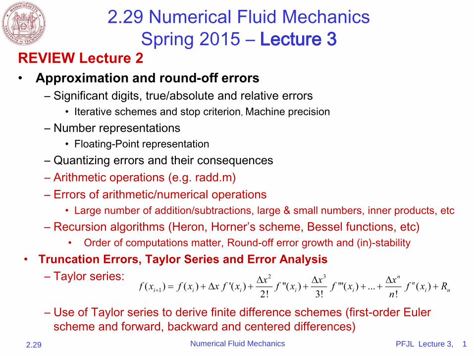
REVIEW Lecture 2• Approximation and round-off errors

– Significant digits, true/absolute and relative errors

• Iterative schemes and stop criterion, Machine precision

– Number representations

• Floating-Point representation

– Quantizing errors and their consequences

– Arithmetic operations (e.g. radd.m)

– Errors of arithmetic/numerical operations

• Large number of addition/subtractions, large & small numbers, inner products, etc

– Recursion algorithms (Heron, Horner’s scheme, Bessel functions, etc)

• Order of computations matter, Round-off error growth and (in)-stability

• Truncation Errors, Taylor Series and Error Analysis – Taylor series:

– Use of Taylor series to derive finite difference schemes (first-order Euler

scheme and forward, backward and centered differences)

2.29 Numerical Fluid Mechanics

Spring 2015 – Lecture 3

2 3

1( ) ( ) '( ) ''( ) '''( ) ... ( )2! 3! !

nn

i i i i i i nx x xf x f x x f x f x f x f x R

n

2.29 Numerical Fluid Mechanics PFJL Lecture 3, 2

2.29 Numerical Fluid Mechanics

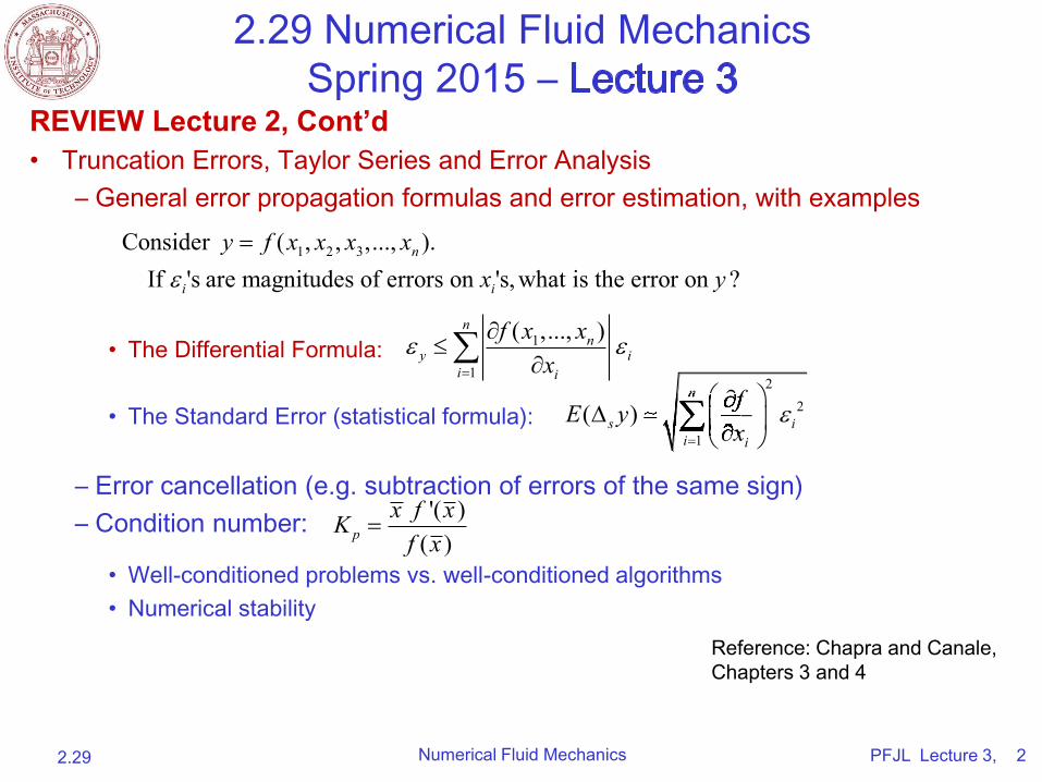
Spring 2015 – Lecture 3REVIEW Lecture 2, Cont’d• Truncation Errors, Taylor Series and Error Analysis

– General error propagation formulas and error estimation, with examples

• The Differential Formula:

• The Standard Error (statistical formula):

– Error cancellation (e.g. subtraction of errors of the same sign)

– Condition number:

• Well-conditioned problems vs. well-conditioned algorithms

• Numerical stability

1 2 3Consider ( , , ,..., ).If 's are magnitudes of errors on 's, what is the error on ?

n

i i

y f x x x xx y

1

1

( ,..., )nn

y ii i

f x xx

22

1

( )n

s ii i

fE yx

1

n

s is is is is if f f ff f

s i s if

f

f f

f f f ff f

f ff fs i s i

s i s i

x x s i s i

s i s i s i s i

s i s i xx xx

s i s i

s i s i

s i s i

s i s is is i

'( )( )p

x f xKf x

Reference: Chapra and Canale, Chapters 3 and 4


Numerical Fluid Mechanics:

Lectures 3 and 4 Outline

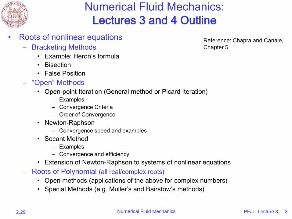
• Roots of nonlinear equations

– Bracketing Methods

• Example: Heron’s formula

• Bisection

• False Position

– “Open” Methods

• Open-point Iteration (General method or Picard Iteration)

– Examples

– Convergence Criteria

– Order of Convergence

• Newton-Raphson

– Convergence speed and examples

• Secant Method

– Examples

– Convergence and efficiency

• Extension of Newton-Raphson to systems of nonlinear equations

– Roots of Polynomial (all real/complex roots)

• Open methods (applications of the above for complex numbers)

• Special Methods (e.g. Muller’s and Bairstow’s methods)

Reference: Chapra and Canale,

Chapter 5


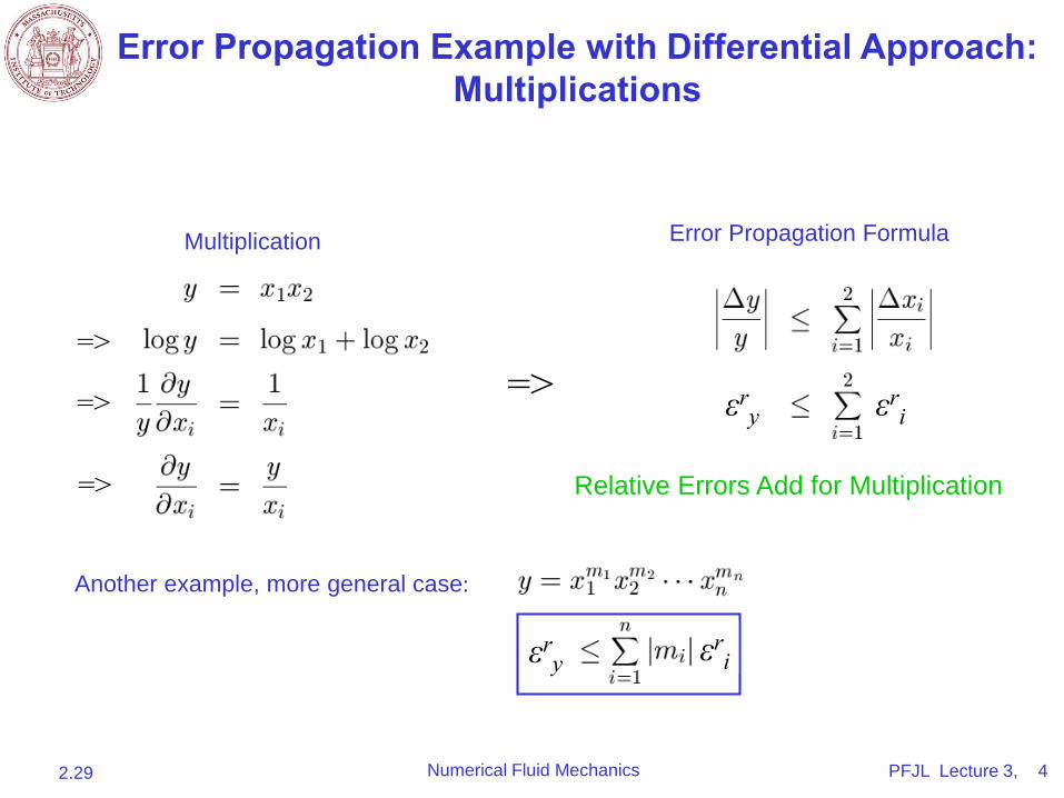
Error Propagation Example with Differential Approach:Multiplications

Multiplication

=>=>

=>

=>

Error Propagation Formula

Relative Errors Add for Multiplication

εry εr

i

Another example, more general case:

εry εr

i


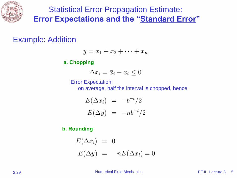
a. Chopping

Example: Addition

Error Expectation:

on average, half the interval is chopped, hence

b. Rounding

Statistical Error Propagation Estimate:

Error Expectations and the “Standard Error”


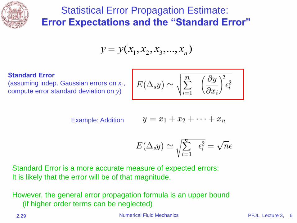
Standard Error(assuming indep. Gaussian errors on xi ,

compute error standard deviation on y)

Standard Error is a more accurate measure of expected errors:

It is likely that the error will be of that magnitude.

However, the general error propagation formula is an upper bound

(if higher order terms can be neglected)

2

n

Statistical Error Propagation Estimate:

Error Expectations and the “Standard Error”

1 2 3( , , ,..., )ny y x x x x

Example: Addition


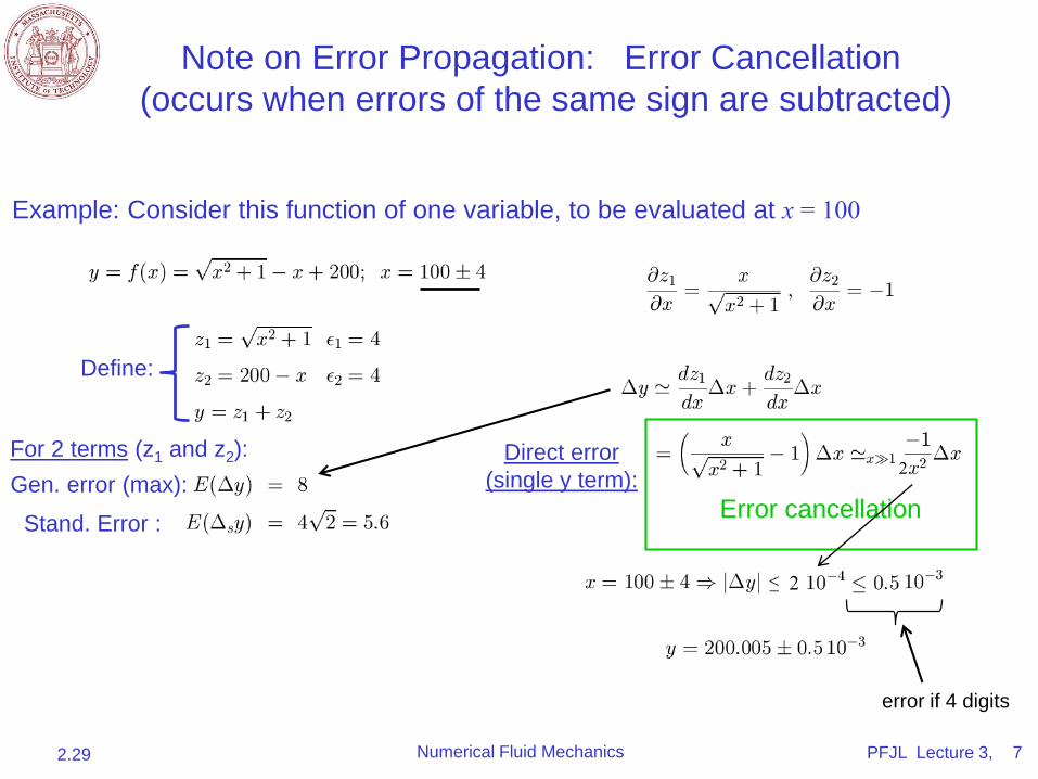
Note on Error Propagation: Error Cancellation

(occurs when errors of the same sign are subtracted)

Example: Consider this function of one variable, to be evaluated at x = 100

Gen. error (max):

Stand. Error :Error cancellation

2

2

Direct error

(single y term):

Define:

For 2 terms (z1 and z2):

error if 4 digits


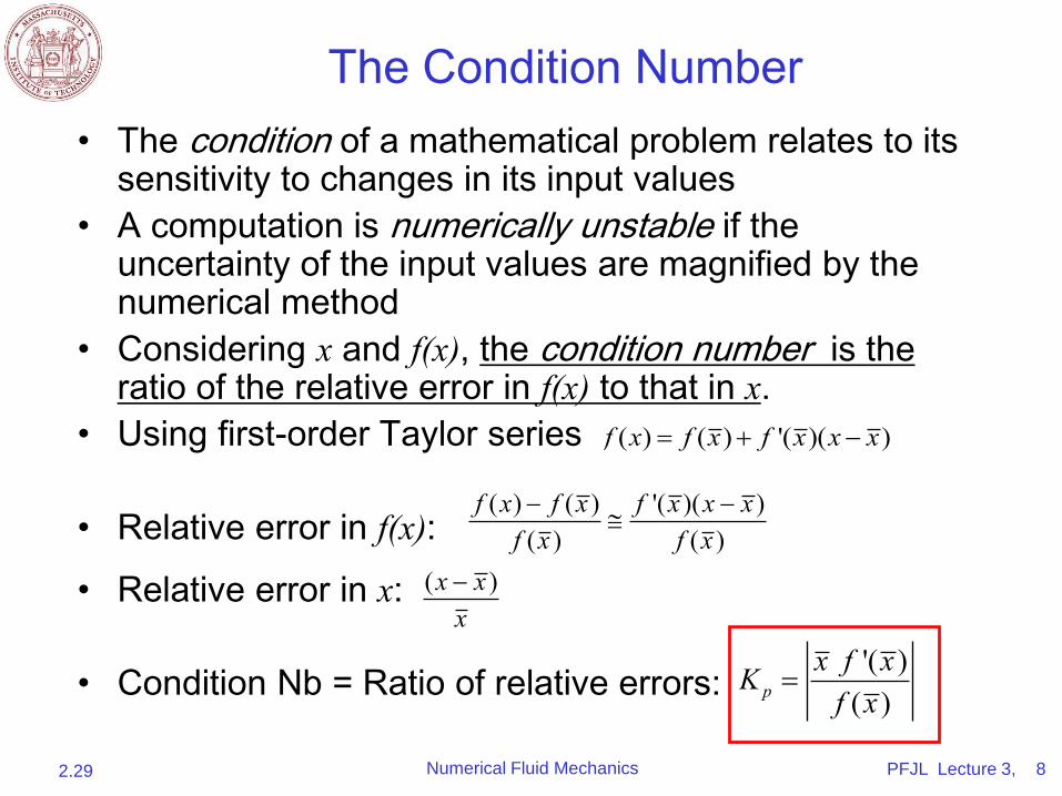
The Condition Number

• The condition of a mathematical problem relates to its sensitivity to changes in its input values

• A computation is numerically unstable if the uncertainty of the input values are magnified by the numerical method

• Considering x and f(x), the condition number is the ratio of the relative error in f(x) to that in x.

• Using first-order Taylor series

• Relative error in f(x):

• Relative error in x:

• Condition Nb = Ratio of relative errors:

( ) ( ) '( )( )f x f x f x x x

( ) ( ) '( )( )( ) ( )

f x f x f x x xf x f x

'( )( )p

x f xKf x

( )x xx


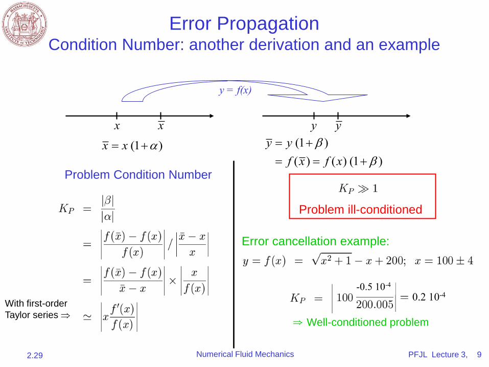
Error PropagationCondition Number: another derivation and an example

xx yy

y = f(x)

Problem ill-conditioned

Error cancellation example:

Problem Condition Number

⇒ Well-conditioned problem

-0.5 10-4

0.2 10-4

(1 )( ) ( ) (1 )

y yf x f x

(1 )x x

With first-order

Taylor series


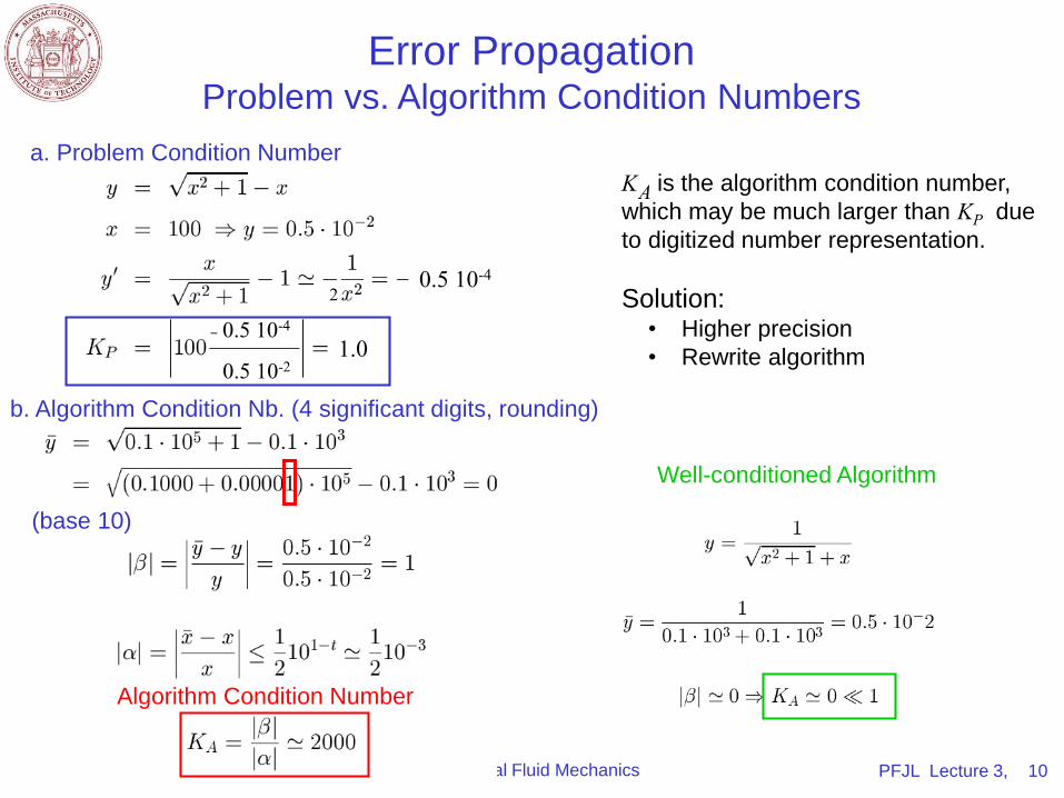
a. Problem Condition Number

b. Algorithm Condition Nb. (4 significant digits, rounding)

Algorithm Condition Number

K is the algorithm condition number,

which may be much larger than KP due

to digitized number representation.

Solution:• Higher precision

• Rewrite algorithm

A

Well-conditioned Algorithm

20.5 10-4

0.5 10-4

1.00.5 10-2

Error PropagationProblem vs. Algorithm Condition Numbers

(base 10)


Roots of Nonlinear Equations

• Finding roots of equations (x | f (x) = 0) ubiquitous in engineering

problems, including numerical fluid dynamics applications

– In general: finding roots of functions (implicit in unknown parameters/roots)

– Fluid Application Examples

• Implicit integration schemes

• Stationary points in fluid equations, stability characterizations, etc

• Fluid dynamical system properties

• Fluid engineering system design

• Most realistic root finding problems require numerical methods

• Two types of root problems/methods:

1.Determine the real roots of algebraic/transcendental equations (these

methods usually need some sort of prior knowledge on a root location)

2.Determine all real and complex roots of polynomials (all roots at once)


Roots of Nonlinear Equations

• Bracketing Methods– Bracket root, systematically reduce width of bracket, track error for

convergence

– Methods: Bisection and False-Position (Regula Falsi)

• “Open” Methods– Systematic “Trial and Error” schemes, don’t require a bracket (can start

from a single value)

– Computationally efficient, but don’t always converge

– Methods: Open-point Iteration (General method or Picard Iteration), Newton-Raphson, Secant Method

– Extension of Newton-Raphson to systems of nonlinear equations

• Roots of Polynomials (all real/complex roots)

– Open methods (applications of the above for complex numbers)

– Special Methods (e.g. Muller’s and Bairstow’s methods)


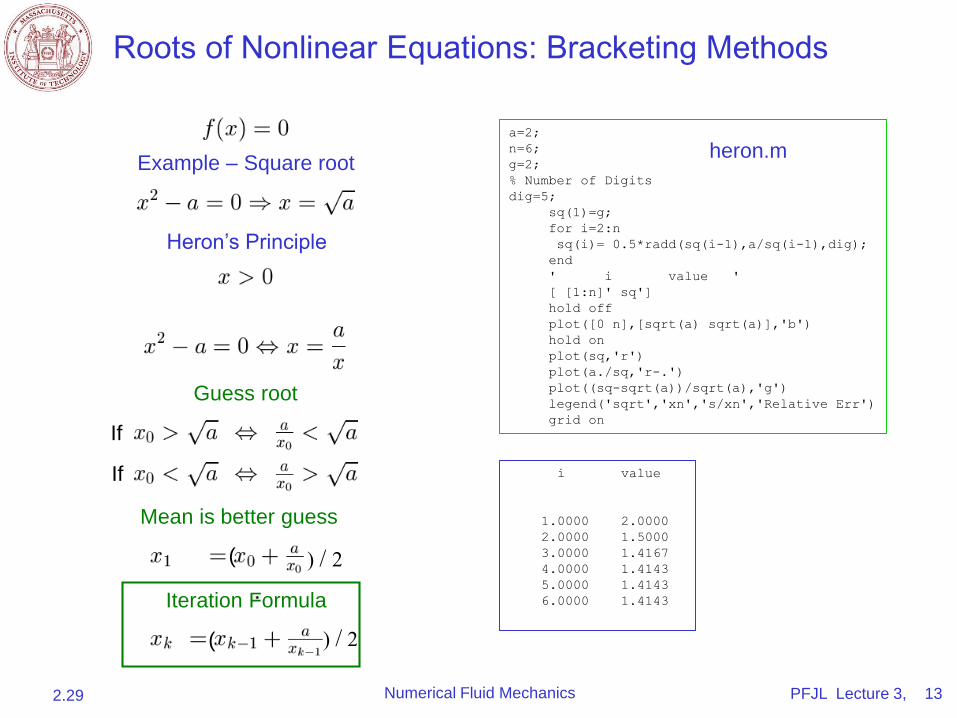
Roots of Nonlinear Equations: Bracketing Methods

Example – Square root

Heron’s Principle

a=2;

n=6;

g=2;

% Number of Digits

dig=5;

sq(1)=g;

for i=2:n

sq(i)= 0.5*radd(sq(i-1),a/sq(i-1),dig);

end

' i value '

[ [1:n]' sq']

hold off

plot([0 n],[sqrt(a) sqrt(a)],'b')

hold on

plot(sq,'r')

plot(a./sq,'r-.')

plot((sq-sqrt(a))/sqrt(a),'g')

legend('sqrt','xn','s/xn','Relative Err')

grid on

heron.m

i value

1.0000 2.0000

2.0000 1.5000

3.0000 1.4167

4.0000 1.4143

5.0000 1.4143

6.0000 1.4143

Guess root

Mean is better guess

Iteration Formula

( ) / 2

( ) / 2

If

If


Bracketing Methods: Graphical Approach

A function typically changes sign at the vicinity of the root “bracket” the root

f(x) f(x) f(x)f(x)

f(x) f(x)

x

xt

xt

xt

xt xt

xa

xa

xa

xa xaxt xa

x

xx x x

(i) (i)(ii) (ii)

(iii) (iv)

Image by MIT OpenCourseWare.

These graphs show general ways in which roots may occur These graphs show some exceptions to the general cases on a bounded interval. In (i) and (ii), if the function is illustrated on the left. In (i), a multiple root occurs where positive at both boundaries, there will be either an even the function is tangential to the x axis. There are an even number of roots or no roots; in the other two graphs, if the number of intersections for the interval. In (ii) is depicted function has opposite signs at the boundary points, there a discontinuous function with an even number of roots will be an odd number of roots within the interval. and end points of opposite signs. Finding the roots in

such cases requires special strategies.



Bisection

x

f(x)

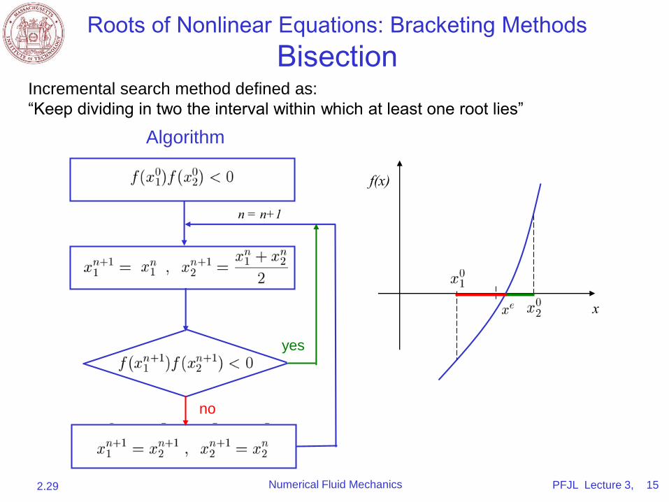
Algorithm

n = n+1

yes

no

Incremental search method defined as:

“Keep dividing in two the interval within which at least one root lies”


n = n+1

yes

no

% Root finding by bi-section

f=inline(' a*x -1','x','a');

a=2

figure(1); clf; hold on

x=[0 1.5]; eps=1e-3;

err=max(abs(x(1)-x(2)),abs(f(x(1),a)-f(x(2),a)));

while (err>eps & f(x(1),a)*f(x(2),a) <= 0)

xo=x; x=[xo(1) 0.5*(xo(1)+xo(2))];

if ( f(x(1),a)*f(x(2),a) > 0 )

x=[0.5*(xo(1)+xo(2)) xo(2)]

end

x

err=max(abs(x(1)-x(2)),abs(f(x(1),a)-f(x(2),a)));

b=plot(x,f(x,a),'.b'); set(b,'MarkerSize',20);

grid on;

end

bisect.m


Bisection

Algorithm

Stop criterion above based on x~0 and f(x)~0

a*x-1=0, with a=2


• Stop criteria:

– absolute added values go to zero: x~0 and f(x)~0

– better to stop when relative estimated error, i.e. relative added

value, is negligible:

• Each successive iteration halves the maximum error, a

general formula thus relates the error and the number of

iterations:

1ˆ ˆ

ˆ

n nr r

a snr

x xx

0

2,

loga d

xnE

0,where is an initial error and the desired errora dx E


Bisection

Numerical Fluid Mechanics2.29

PFJL Lecture 3, 18

Another Bracketing Method:

The False Position Method (Regula Falsi)

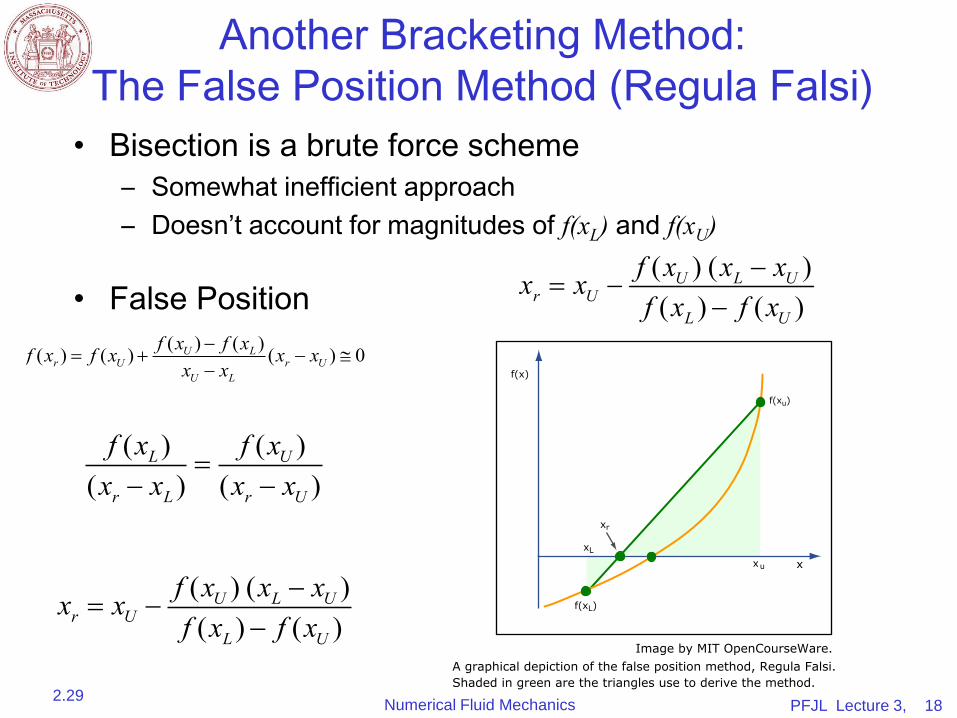
• Bisection is a brute force scheme

– Somewhat inefficient approach

– Doesn’t account for magnitudes of f(xL) and f(xU)

• False Position

( ) ( )( ) ( )

L U

r L r U

f x f xx x x x

( ) ( )( ) ( )

U L Ur U

L U

f x x xx xf x f x

( ) ( )( ) ( ) ( ) 0U Lr U r U

U L

f x f xf x f x x xx x

f x( )x U ( x L x U )r xU f x( ) L f x( U )

f(x)

f(xL)

f(xu)

xr

xL

xu x

Image by MIT OpenCourseWare.A graphical depiction of the false position method, Regula Falsi.Shaded in green are the triangles use to derive the method.


Comments on Bracketing Methods

(Bisection and False Postion)

• Bisection and False Position:

– Convergent methods, but can be slow and thus can require lots of

function evaluations, each of which can be very expensive (full code).

• Error of False Position can decrease much faster than that of

Bisection, but if the function is far from a straight line, False

Position will be slow (one of the end point remains fixed)

• Remedy: “Modified False Position”

– e.g. if end point remains fixed for a few iterations, reduce end-point

function value at end point, e.g. divide interval by 2

• One can not really generalize behaviors for Root Finding

methods (results are function dependent)

• Always substitute estimate of root xr at the end to check how

close estimate is to f(xr)=0


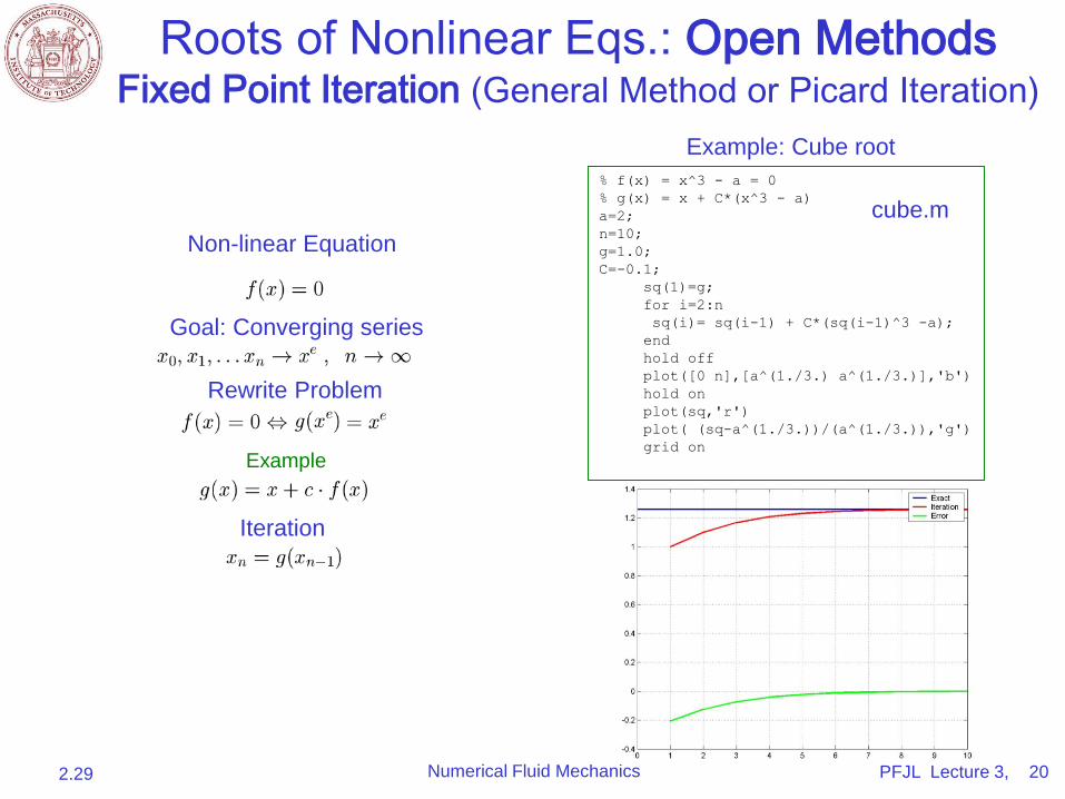
Roots of Nonlinear Eqs.: Open MethodsFixed Point Iteration (General Method or Picard Iteration)

Non-linear Equation

Goal: Converging series

Rewrite Problem

Example

Iteration

% f(x) = x^3 - a = 0

% g(x) = x + C*(x^3 - a)

a=2;

n=10;

g=1.0;

C=-0.1;

sq(1)=g;

for i=2:n

sq(i)= sq(i-1) + C*(sq(i-1)^3 -a);

end

hold off

plot([0 n],[a^(1./3.) a^(1./3.)],'b')

hold on

plot(sq,'r')

plot( (sq-a^(1./3.))/(a^(1./3.)),'g')

grid on

cube.m

Example: Cube root


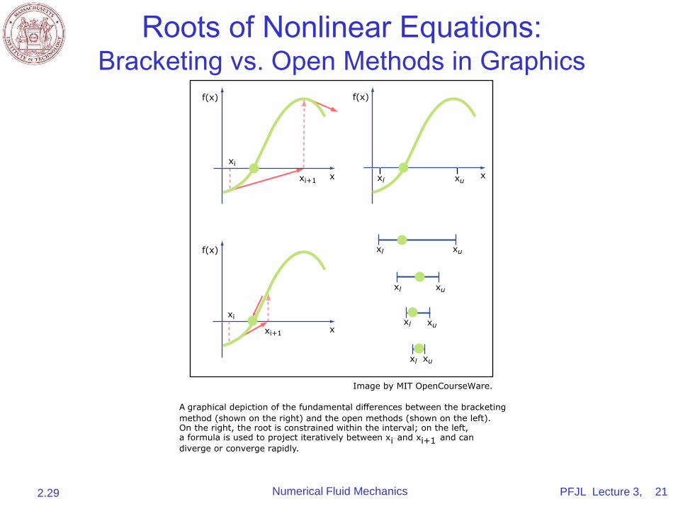
Roots of Nonlinear Equations: Bracketing vs. Open Methods in Graphics

A graphical depiction of the fundamental differences between the bracketing method (shown on the right) and the open methods (shown on the left). On the right, the root is constrained within the interval; on the left, a formula is used to project iteratively between x and x and can i i+1 diverge or converge rapidly.

f(x)

xl xux

xl xu

xl xu

xl xu

xl xu

f(x)

xi

xi+1 x

f(x)

xi

xi+1 x

Image by MIT OpenCourseWare.


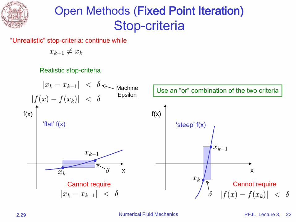
Open Methods (Fixed Point Iteration)

Stop-criteria“Unrealistic” stop-criteria: continue while

Realistic stop-criteria

Machine

Epsilon

x

f(x)

‘flat’ f(x)

d x

f(x)

‘steep’ f(x)

d

Cannot require Cannot require

Use an “or” combination of the two criteria

MIT OpenCourseWarehttp://ocw.mit.edu

2.29 Numerical Fluid MechanicsSpring 2015

For information about citing these materials or our Terms of Use, visit: http://ocw.mit.edu/terms.

http://ocw.mit.edu/terms

http://ocw.mit.edu/

REVIEW Lecture 2 - MIT OpenCourseWare Numerical Fluid Mechanics PFJL Lecture 3, 11. Roots of Nonlinear Equations •Finding roots of equations (x | f (x) = 0) ubiquitous in engineering

Documents