Review for Exam 2. Section 14 - Michigan State University

Review for Exam 2.

I Sections 13.1, 13.3. 14.1-14.7.

I 50 minutes.

I 5 problems, similar to homework problems.

I No calculators, no notes, no books, no phones.

I No green book needed.

Section 14.7

Example

(a) Find all the critical points of f (x , y) = 12xy − 2x3 − 3y2.

(b) For each critical point of f , determine whether f has a localmaximum, local minimum, or saddle point at that point.

Solution:(a) ∇f (x , y) = 〈12y − 6x2, 12x − 6y〉 = 〈0, 0〉, then,

x2 = 2y , y = 2x , ⇒ x(x − 4) = 0.

There are two solutions, x = 0 ⇒ y = 0, and x = 4 ⇒ y = 8.That is, there are two critical points, (0, 0) and (4, 8).

Section 14.7

Example

(a) Find all the critical points of f (x , y) = 12xy − 2x3 − 3y2.

(b) For each critical point of f , determine whether f has a localmaximum, local minimum, or saddle point at that point.

Solution:(b) Recalling ∇f (x , y) = 〈12y − 6x2, 12x − 6y〉, we compute

fxx = −12x , fyy = −6, fxy = 12.

D(x , y) = fxx fyy − (fxy )2 = 144(x

2− 1

),

Since D(0, 0) = −144 < 0, the point (0, 0) is a saddle point of f .

Since D(4, 8) = 144(2− 1) > 0, and fxx(4, 8) = (−12)4 < 0, thepoint (4, 8) is a local maximum of f . C

Section 14.7

Example

Find the absolute maximum and absolute minimum of

f (x , y) = 2 + xy − 2x − 1

4y2 in the closed triangular region with

vertices given by (0, 0), (1, 0), and (0, 2).

Solution:We start finding the critical points inside the triangular region.

∇f (x , y) =⟨y − 2, x − 1

2y⟩

= 〈0, 0〉, ⇒ y = 2, y = 2x .

The solution is (1, 2). This point is outside in the triangular regiongiven by the problem, so there is no critical point inside the region.

Section 14.7

Example


f (x , y) = 2 + xy − 2x − 1



Solution:We now find the candidates for absolute maximum and minimumon the borders of the triangular region. We first record theboundary vertices:

(0, 0) ⇒ f (0, 0) = 2,

(1, 0) ⇒ f (1, 0) = 0,

(0, 2) ⇒ f (0, 2) = 1.

Section 14.7

Example


f (x , y) = 2 + xy − 2x − 1



Solution:

I The horizontal side of the triangle, y = 0, x ∈ (0, 1). Since

g(x) = f (x , 0) = 2− 2x , ⇒ g ′(x) = −2 6= 0.

there are no candidates in this part of the boundary.

I The vertical side of the triangle is x = 0, y ∈ (0, 2). Then,

g(y) = f (0, y) = 2− 1

4y2, ⇒ g ′(y) = −1

2y = 0,

so y = 0 and we recover the point (0, 0).

Section 14.7

Example


f (x , y) = 2 + xy − 2x − 1



Solution:

I The hypotenuse of the triangle y = 2− 2x , x ∈ (0, 1). Then,

g(x) = f (x , 2− 2x) = 2 + x(2− 2x)− 2x − 1

4(2− 2x)2,

= 2 + 2x − 2x2 − 2x − (x2 − 2x + 1),

= 1 + 2x − 3x2.

Then, g ′(x) = 2− 6x = 0 implies x = 13 , hence y = 4

3 . Thecandidate is

(13 , 4

3

).

Section 14.7

Example


f (x , y) = 2 + xy − 2x − 1



Solution:

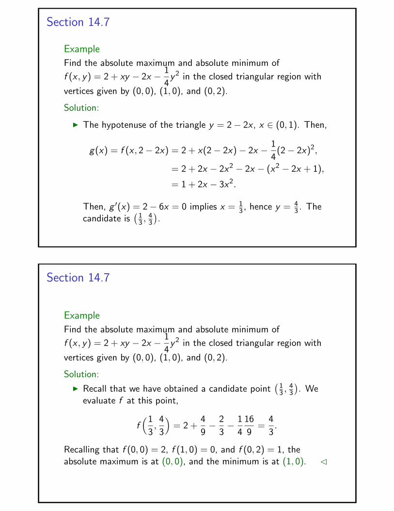
I Recall that we have obtained a candidate point(

13 , 4

3

). We

evaluate f at this point,

f(1

3,4

3

)= 2 +

4

9− 2

3− 1

4

16

9=

4

3.

Recalling that f (0, 0) = 2, f (1, 0) = 0, and f (0, 2) = 1, theabsolute maximum is at (0, 0), and the minimum is at (1, 0). C

Section 14.6

Example

(a) Find the linear approximation L(x , y) of the functionf (x , y) = sin(2x + 3y) + 1 at the point (−3, 2).

(b) Use the approximation above to estimate the value off (−2.8, 2.3).

Solution:(a) L(x , y) = fx(−3, 2) (x + 3) + fy (−3, 2) (y − 2) + f (−3, 2).

Since fx(x , y) = 2 cos(2x + 3y) and fy (x , y) = 3 cos(2x + 3y),

fx(−3, 2) = 2 cos(−6 + 6) = 2,

fy (−3, 2) = 3 cos(−6 + 6) = 3,

f (−3, 2) = sin(−6 + 6) + 1 = 1.

the linear approximation is L(x , y) = 2(x + 3) + 3(y − 2) + 1.

Section 14.6

Example

(a) Find the linear approximation L(x , y) of the functionf (x , y) = sin(2x + 3y) + 1 at the point (−3, 2).

(b) Use the approximation above to estimate the value off (−2.8, 2.3).

Solution:(b) Recall: L(x , y) = 2(x + 3) + 3(y − 2) + 1.Now, the linear approximation of f (−2.8, 2.3) is L(−2.8, 2.3), and

L(−2.8, 2.3) = 2(−2.8 + 3) + 3(2.3− 2) + 2

= 2(0.2) + 3(0.3) + 1

= 2.3.

We conclude L(−2.8, 2.3) = 2.3. C

Section 14.5

Example

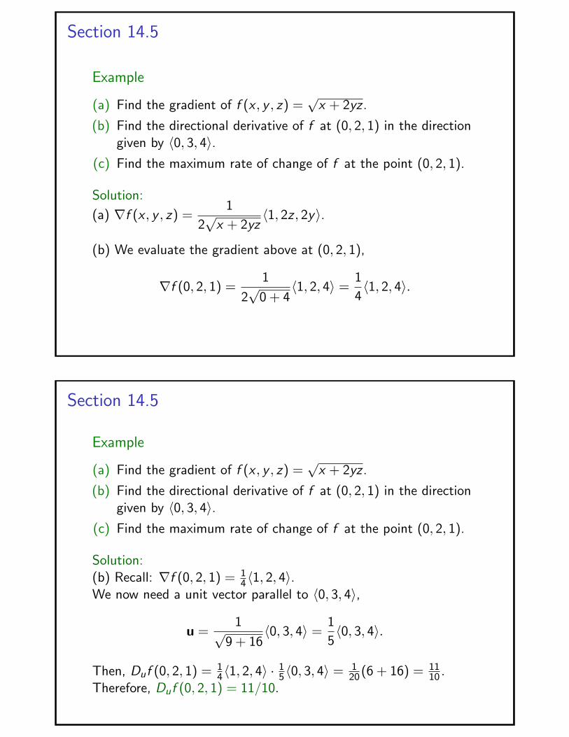
(a) Find the gradient of f (x , y , z) =√

x + 2yz .

(b) Find the directional derivative of f at (0, 2, 1) in the directiongiven by 〈0, 3, 4〉.

(c) Find the maximum rate of change of f at the point (0, 2, 1).

Solution:

(a) ∇f (x , y , z) =1

2√

x + 2yz〈1, 2z , 2y〉.

(b) We evaluate the gradient above at (0, 2, 1),

∇f (0, 2, 1) =1

2√

0 + 4〈1, 2, 4〉 =

1

4〈1, 2, 4〉.

Section 14.5

Example


x + 2yz .



Solution:(b) Recall: ∇f (0, 2, 1) = 1

4〈1, 2, 4〉.We now need a unit vector parallel to 〈0, 3, 4〉,

u =1√

9 + 16〈0, 3, 4〉 =

1

5〈0, 3, 4〉.

Then, Duf (0, 2, 1) = 14〈1, 2, 4〉 · 1

5〈0, 3, 4〉 = 120(6 + 16) = 11

10 .Therefore, Duf (0, 2, 1) = 11/10.

Section 14.5

Example


x + 2yz .



Solution:(c) The maximum rate of change of f at a point is the magnitudeof its gradient at that point, that is,

|∇f (0, 2, 1)| = 1

4|〈1, 2, 4〉| = 1

4

√1 + 4 + 16 =

√21

4.

Therefore, the maximum rate of change of the function f at thepoint (0, 2, 1) is given by

√21/4. C

Section 14.3

Example

Find any value of the constant a such that the functionf (x , y) = e−ax cos(y)− e−y cos(x) is solution of Laplace’sequation fxx + fyy = 0.

Solution:

fx = −ae−ax cos(y) + e−y sin(x), fy = −e−ax sin(y) + e−y cos(x),

fxx = a2e−ax cos(y) + e−y cos(x), fyy = −e−ax cos(y)− e−y cos(x),

then

fxx + fyy =[a2e−ax cos(y) + e−y cos(x)

]+

[−e−ax cos(y)− e−y cos(x)

],

= (a2 − 1)e−ax cos(y).

Function f is solution of fxx + fyy = 0 iff a = ±1. C

Section 14.2

Example

Compute the limit lim(x ,y)→(0,0)

x2 sin2(y)

2x2 + 3y2.

Solution:

Since x2 6 2x2 + 3y2, that is,x2

2x2 + 3y26 1, the non-negative

function f (x , y) =x2 sin2(y)

2x2 + 3y2satisfies the bounds

0 6 f (x , y) 6 sin2(y).

Since limy→0 sin2(y) = 0, the Sandwich Theorem implies that

lim(x ,y)→(0,0)

x2 sin2(y)

2x2 + 3y2= 0.

C

Section 13.3Example

Reparametrize the curve r(t) =⟨3

2sin(t2), 2t2,

3

2cos(t2)

⟩with

respect to its arc length measured from t = 1 in the direction ofincreasing t.

Solution:We first compute the arc length function. We start with thederivative

r′(t) = 〈3t cos(t2), 4t,−3 sin(t2)〉,

We now need its magnitude,

|r′(t)| =√

9t2 cos2(t2) + 16t2 + 9 sin2(t2),

=√

9t2 + 16t2,

=√

9 + 16t,

= 5t.

Section 13.3

Example

Reparametrize the curve r(t) =⟨3

2sin(t2), 2t2,

3

2cos(t2)

⟩with

respect to its arc length measured from t = 1 in the direction ofincreasing t.

Solution:Recall: |r′(t)| = 5t. Then, the arc length function is

s(t) =

∫ t

15τ dτ =

5

2

(τ2

∣∣∣t1

)=

5

2(t2 − 1).

Inverting this function for t2, we obtain t2 =2

5s + 1. The

reparametrization of r(t) is given by

r(s) =⟨3

2sin

(2

5s + 1

), 2

(2

5s + 1

),3

2cos

(2

5s + 1

)⟩.

C

Double integrals (Sect. 15.1)

I Review: Integral of a single variable function.

I Double integral on rectangles.

I Fubini Theorem on rectangular domains.

I Examples.

Next class:

I Double integrals over non-rectangular regions.

I Fubini Theorem on non-rectangular domains.

I Finding the limits of integration.

Review: Integral of a single variable function.

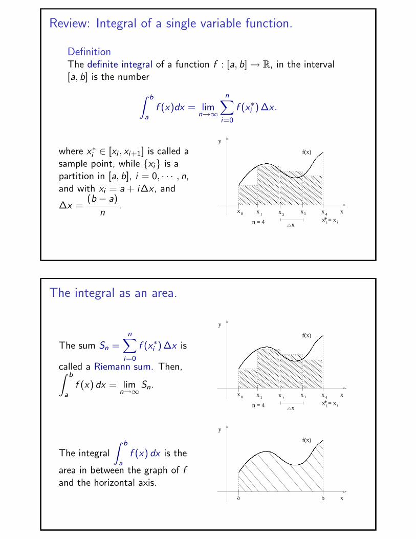
DefinitionThe definite integral of a function f : [a, b] → R, in the interval[a, b] is the number∫ b

af (x)dx = lim

n→∞

n∑i=0

f (x∗i ) ∆x .

where x∗i ∈ [xi , xi+1] is called asample point, while {xi} is apartition in [a, b], i = 0, · · · , n,and with xi = a + i∆x , and

∆x =(b − a)

n.

i

��

��

��

��

��

��

��

��

y

f(x)

x

x 1x 0 x 2

x3 x 4

n = 4 x = x

x*

i

The integral as an area.

The sum Sn =n∑

i=0

f (x∗i ) ∆x is

called a Riemann sum. Then,∫ b

af (x) dx = lim

n→∞Sn.

i

��

��

��

��

��

��

��

��

y

f(x)

x

x 1x 0 x 2

x3 x 4

n = 4 x = x

x*

i

The integral

∫ b

af (x) dx is the

area in between the graph of fand the horizontal axis.

b

y

f(x)

xa





I Examples.

Double integrals on rectangles

DefinitionThe double integral of a function f : R ⊂ R2 → R in the rectangleR = [a, b]× [c , d ] is the number∫∫

Rf (x , y) dx dy = lim

n→∞

n∑i=0

n∑j=0

f (x∗i , y∗j ) ∆x∆y .

where x∗i ∈ [xi , xi+1], y∗j = [yj , yj+1],are sample points, while {xi} and {yj},i , j = 0, · · · , n are partitions of theintervals [a, b] and [c , d ], and

∆x =(b − a)

n, ∆y =

(d − c)

n. x

y y y

xx

xx

x

y

0

0 4

4

1

1y

2

2 3

3

z

R

y

The double integral as a volume.

The sum

Sn = limn→∞

n∑i=0

n∑j=0

f (x∗i , y∗j ) ∆x∆y is

called a Riemann sum. Then,∫∫R

f (x , y) dx dy = limn→∞

Sn.x

y y y

xx

xx

x

y

0

0 4

4

1

1y

2

2 3

3

z

R

y

The integral

∫∫R

f (x , y) dx dy is

the volume above R and belowthe graph of f .

y

R

zf(x,y)

x





I Examples.

Fubini Theorem on rectangular domains.

TheoremIf f : R ⊂ R2 → R is continuous in R = [x0, x1]× [y0, y1], then∫∫

Rf (x , y) dx dy =

∫ y1

y0

[∫ x1

x0

f (x , y) dx]dy ,

=

∫ x1

x0

[∫ y1

y0

f (x , y) dy]dx .

Remark: Fubini’s Theorem: The order of integration can beswitched in double integrals of continuous functions on a rectangle.

Notation: The double integral is also written as∫∫R

f (x , y) dx dy =

∫ y1

y0

∫ x1

x0

f (x , y) dx dy .


Example

Use Fubini’s Theorem to compute the double integral∫∫R

f (x , y) dx dy , where f (x , y) = xy2 + 2x2y3, and

R = [0, 2]× [1, 3]. Integrate first in x , then in y .

Solution: Since x ∈ [0, 2] and y ∈ [1, 3],∫∫R

f (x , y) dx dy =

∫ 3

1

∫ 2

0(xy2 + 2x2y3)dx dy

=

∫ 3

1

[∫ 2

0(xy2 + 2x2y3)dx

]dy .

We compute the interior integral in x first, keeping y constant.After that we compute the integral in y .


Example




Solution: We compute the integral in x first, keeping y constant.∫∫R

f (x , y) dx dy =

∫ 3

1

[∫ 2

0(xy2 + 2x2y3)dx

]dy

=

∫ 3

1

[y2

2

(x2

∣∣∣20

)+

2y3

3

(x3

∣∣∣20

)]dy ,

=

∫ 3

1

[2y2 +

16

3y3

]dy .

We now compute the integral in y ,


Example




Solution: We now compute the integral in y ,∫∫R

f (x , y) dx dy =

∫ 3

1

[2y2 +

16

3y3

]dy ,

= 2y3

3

∣∣∣31+

16

3

y4

4

∣∣∣31.

We conclude:

∫∫R

f (x , y) dx dy = 226

3+

4

380 = 372/3. C


Example



R = [0, 2]× [1, 3]. Integrate first in y , then in x .

Solution:∫∫R

f (x , y) dx dy =

∫ 3

1

∫ 2

0(xy2 + 2x2y3)dx dy

=

∫ 2

0

[∫ 3

1(xy2 + 2x2y3)dy

]dx .

∫∫R

f (x , y) dx dy =

∫ 2

0

[x

3

(y3

∣∣∣31

)+

2x2

4

(y4

∣∣∣31

)]dx .


Example




Solution:

∫∫R

f (x , y) dx dy =

∫ 2

0

[x

3

(y3

∣∣∣31

)+

2x2

4

(y4

∣∣∣31

)]dx .

∫∫R

f (x , y) dx dy =

∫ 2

0

[26

3x + 40 x2

]dx

=26

3

x2

2

∣∣∣20+ 40

x3

3

∣∣∣20

=26

3(2) + 40

8

3⇒

∫∫R

f (x , y) dx dy = 372/3.


Example


f (x , y) dx dy , where f (x , y) =x

y+

y

x, and R = [1, 4]× [1, 2].

Solution: We choose to first integrate in y and then in x .∫∫R

f (x , y) dx dy =

∫ 4

1

∫ 2

1

(x

y+

y

x

)dy dx ,

=

∫ 4

1

[∫ 2

1

(x

y+

y

x

)dy

]dx ,

=

∫ 4

1

[x(ln(y)

∣∣∣21

)+

1

x

(y2

2

∣∣∣21

)]dx ,

=

∫ 4

1

[ln(2) x +

3

2

1

x

]dx .


Example


f (x , y) dx dy , where f (x , y) =x

y+

y

x, and R = [1, 4]× [1, 2].

Solution: We compute the integral in x ,∫∫R

f (x , y) dx dy =

∫ 4

1

[ln(2) x +

3

2

1

x

]dx

= ln(2)(x2

2

∣∣∣41

)+

3

2

(ln(x)

∣∣∣41

),

=15

2ln(2) +

3

2ln(4),

=

(15

2+ 3

)ln(2).

We conclude:

∫∫R

f (x , y) dx dy = (21/2) ln(2). C

A particular case of Fubini’s Theorem.

Corollary

If the continuous function f : R ⊂ R2 → R satisfies thatf (x , y) = g(x)h(y), then the double integral of function f in therectangle R = [x0, x1]× [y0, y1] is given by∫ x1

x0

∫ y1

y0

g(x)h(y)dy dx =(∫ x1

x0

g(x)dx)(∫ y1

y0

h(y)dy).

Remark: In the case that f (x , y) is a product of two functions g ,h, with g(x) and h(y), then the double integral of f is also aproduct of the integral of g times the integral of h.

A particular case of Fubini’s Theorem.

Example

Compute the double integral of f (x , y) =1 + x2

1 + y2, in the

rectangular region R = [0, 2]× [0, 1].

Solution:∫∫R

f (x , y) dx dy =

∫ 2

0

∫ 1

0

1 + x2

1 + y2dy dx ,

=[∫ 2

0(1 + x2)dx

][∫ 1

0

1

1 + y2dy

],

=(x∣∣∣20+

1

3x∣∣∣20

)(arctan(y)

∣∣∣10

),

=π

4

(2 +

8

3

).

We conclude

∫∫R

f (x , y) dx dy = (14/3)(π/4) = (7/6)π. C

Double integrals on regions (Sect. 15.1)

I Review: Fubini’s Theorem on rectangular domains.I Fubini’s Theorem on non-rectangular domains.

I Type I: Domain functions y(x).I Type II: Domain functions x(y).


Review: Fubini’s Theorem on rectangular domains.

TheoremIf f : R ⊂ R2 → R is continuous in R = [a, b]× [c , d ], then∫∫

Rf (x , y) dx dy =

∫ b

a

∫ d

cf (x , y) dy dx ,

=

∫ d

c

∫ b

af (x , y) dx dy .

Remark: Fubini’s Theorem: It issimple to switch the order ofintegration in double integrals ofcontinuous functions on arectangle.

y

R

zf(x,y)

x





Fubini’s Theorem on Type I domains, y(x).

TheoremIf f : D ⊂ R2 → R is continuous in D, then hold (Type I):If D =

{(x , y) ∈ R2 : x ∈ [a, b], y ∈ [g1(x), g2(x)]

}, with g1, g2

continuous functions on [a, b], then∫∫D

f (x , y) dx dy =

∫ b

a

∫ g2(x)

g1(x)f (x , y) dy dx .

1

y2

xa b

y = g (x)

x

y = g (x)b

z

x

f(x,y)

y

f(x,g (x)) f(x,g (x))

g (x)g (x)

1

1 2

2

a





Fubini’s Theorem on Type II domains, x(y).

TheoremIf f : D ⊂ R2 → R is continuous in D, then hold (Type II):If D =

{(x , y) ∈ R2 : x ∈ [h1(y), h2(y)], y ∈ [c , d ]

}, with h1, h2

continuous functions on [c , d ], then∫∫D

f (x , y) dx dy =

∫ d

c

∫ h2(y)

h1(y)f (x , y) dx dy .

2

y

x

y

d

c

x = h (y) x = h (y)1

c

h (y)

h (y)

2

1

x

y

z f(x,y)

f(h (y),y)

f(h (y),y)2

1

d

Summary: Fubini’s Theorem on non-rectangular domains.

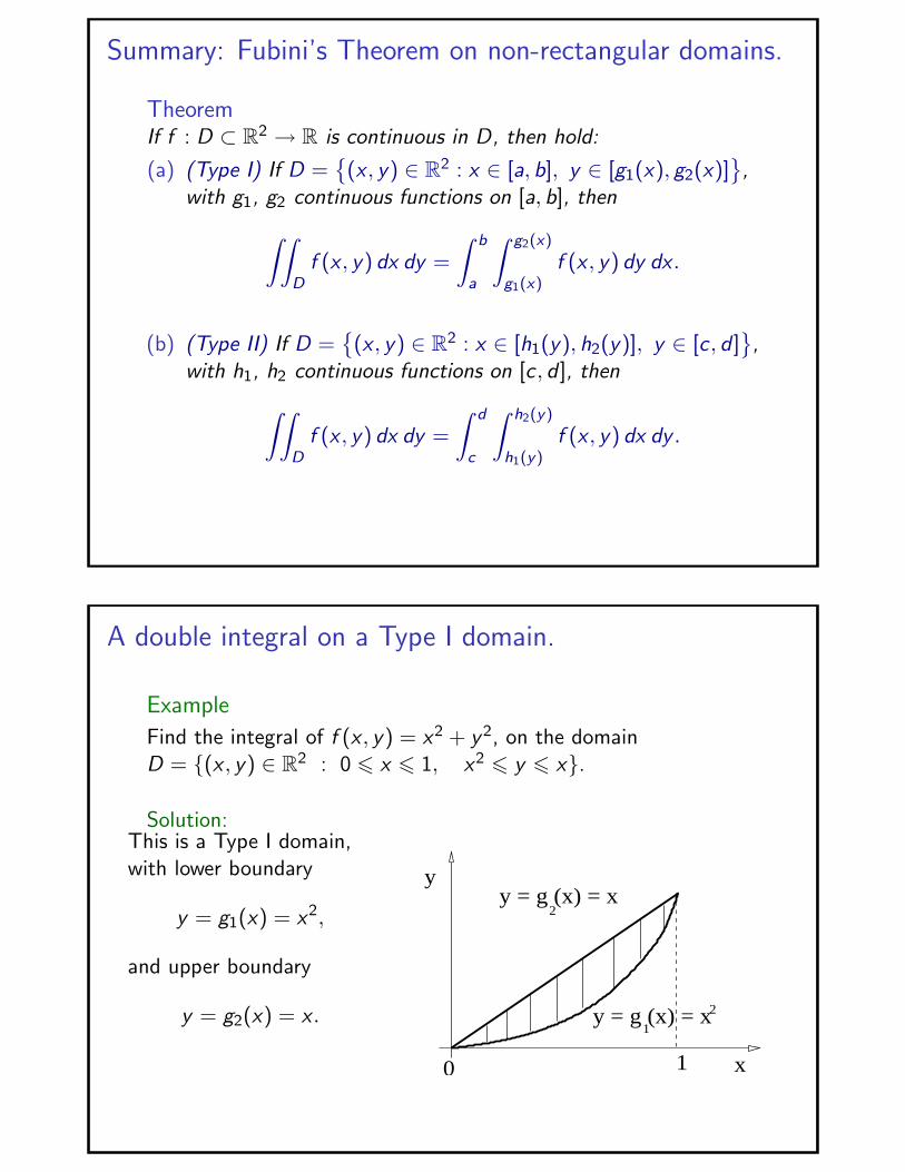
TheoremIf f : D ⊂ R2 → R is continuous in D, then hold:

(a) (Type I) If D ={(x , y) ∈ R2 : x ∈ [a, b], y ∈ [g1(x), g2(x)]

},

with g1, g2 continuous functions on [a, b], then∫∫D

f (x , y) dx dy =

∫ b

a

∫ g2(x)


(b) (Type II) If D ={(x , y) ∈ R2 : x ∈ [h1(y), h2(y)], y ∈ [c , d ]

},

with h1, h2 continuous functions on [c , d ], then∫∫D

f (x , y) dx dy =

∫ d

c

∫ h2(y)


A double integral on a Type I domain.

Example

Find the integral of f (x , y) = x2 + y2, on the domainD = {(x , y) ∈ R2 : 0 6 x 6 1, x2 6 y 6 x}.

Solution:This is a Type I domain,with lower boundary

y = g1(x) = x2,

and upper boundary

y = g2(x) = x . 2

10

y = g (x) = x 2

y

x

y = g (x) = x1


Example


Solution: Recall:

∫∫D

f (x , y) dx dy =

∫ b

a

∫ g2(x)

g1(x)f (x , y) dy dx

with g1(x) = x2 and g2(x) = x , we obtain∫∫D

f (x , y) dx dy =

∫ 1

0

∫ x

x2

(x2 + y2)dy dx ,

=

∫ 1

0

[x2

(y∣∣∣xx2

)+

(y3

3

∣∣∣xx2

)]dx .

∫∫D

f (x , y) dx dy =

∫ 1

0

[x2

(x − x2

)+

1

3

(x3 − x6

)]dx .


Example


Solution:

∫∫D

f (x , y) dx dy =

∫ 1

0

[x2

(x − x2

)+

1

3

(x3 − x6

)]dx .

∫∫D

f (x , y) dx dy =

∫ 1

0

[x3 − x4 +

1

3x3 − 1

3x6

]dx ,

=[x4

4− x5

5+

x4

12− x7

21

]∣∣∣10,

=1

3− 1

5− 1

21=

9

(3)(5)(7).

We conclude:

∫∫D

f (x , y) dx dy =3

35. C

Summary: Fubini’s Theorem on non-rectangular domains.

TheoremIf f : D ⊂ R2 → R is continuous in D, then hold:

(a) (Type I) If D ={(x , y) ∈ R2 : x ∈ [a, b], y ∈ [g1(x), g2(x)]

},

with g1, g2 continuous functions on [a, b], then∫∫D

f (x , y) dx dy =

∫ b

a

∫ g2(x)


(b) (Type II) If D ={(x , y) ∈ R2 : x ∈ [h1(y), h2(y)], y ∈ [c , d ]

},

with h1, h2 continuous functions on [c , d ], then∫∫D

f (x , y) dx dy =

∫ d

c

∫ h2(y)


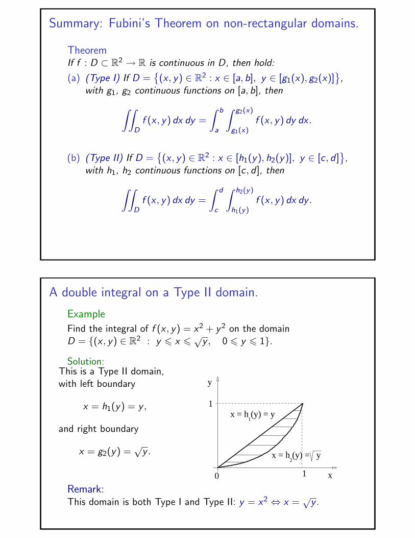
A double integral on a Type II domain.

Example

Find the integral of f (x , y) = x2 + y2 on the domainD = {(x , y) ∈ R2 : y 6 x 6

√y , 0 6 y 6 1}.

Solution:This is a Type II domain,with left boundary

x = h1(y) = y ,

and right boundary

x = g2(y) =√

y .

x10

1x = h (y) = y

1

2x = h (y) = y

y

Remark:This domain is both Type I and Type II: y = x2 ⇔ x =

√y .


Example

Find the integral of f (x , y) = x2 + y2, on the domainD = {(x , y) ∈ R2 : y 6 x 6

√y , 0 6 y 6 1}.

Solution: Recall:

∫∫D

f (x , y) dx dy =

∫ d

c

∫ h2(y)

h1(y)f (x , y) dx dy

with h1(y) = y and h2(y) =√

y , we obtain∫∫D

f (x , y) dx dy =

∫ 1

0

∫ √y

y

(x2 + y2

)dx dy ,

=

∫ 1

0

[(x3

3

∣∣∣√y

y

)+ y2

(x∣∣∣√y

y

)]dy .

∫∫D

f (x , y) dx dy =

∫ 1

0

[1

3

(y3/2 − y3

)+ y2

(y1/2 − y

)]dy .


Example

Find the integral of f (x , y) = x2 + y2, on the domainD = {(x , y) ∈ R2 : y 6 x 6

√y , 0 6 y 6 1}.

Solution:∫∫D

f (x , y) dx dy =

∫ 1

0

[1

3

(y3/2 − y3

)+ y2

(y1/2 − y

)]dy .

∫∫D

f (x , y) dx dy =

∫ 1

0

[1

3y3/2 − 1

3y3 + y5/2 − y3

]dy ,

=[1

3

2

5y5/2 − 1

3

y4

4+

2

7y7/2 − y4

4

]∣∣∣10,

=2

15− 1

12+

2

7− 1

4=

9

(3)(5)(7).

We conclude

∫∫D

f (x , y) dx dy =3

35. C

Domains Type I and Type II.

Summary: We have shown that a double integral of a function fon the domain D given in the pictures below holds,∫∫

Df (x , y)dx dy =

∫ 1

0

∫ x

x2

f (x , y)dy dx =

∫ 1

0

∫ √y

yf (x , y)dx dy .

2

10

y = g (x) = x 2

y

x

y = g (x) = x1

x10

1x = h (y) = y

1

2x = h (y) = y

y





Domains Type I and Type II.Example

Find the limits of integration of∫ ∫

D f (x , y) dxdy in the domain

D ={(x , y) ∈ R2 :

x2

9+

y2

46 1

}when D is considered first as

Type I and then as Type II.

Solution: The boundary is the ellipsex2

9+

y2

4= 1.

So, the boundary as Type I is given by

y = −2

√1− x2

9= g1(x), y = 2

√1− x2

9= g2(x).

The boundary as Type II is given by

x = −3

√1− y2

4= h1(y), x = 3

√1− y2

4= h2(y).

C

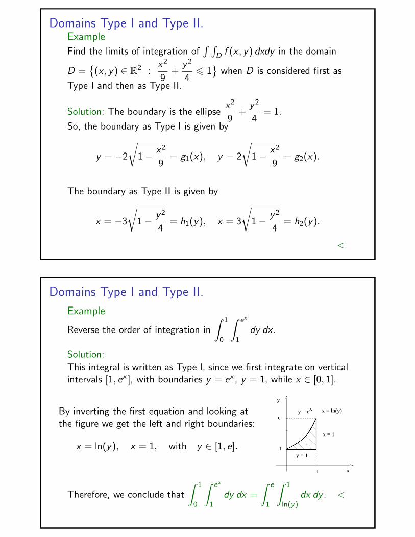
Domains Type I and Type II.

Example

Reverse the order of integration in

∫ 1

0

∫ ex

1dy dx .

Solution:This integral is written as Type I, since we first integrate on verticalintervals [1, ex ], with boundaries y = ex , y = 1, while x ∈ [0, 1].

By inverting the first equation and looking atthe figure we get the left and right boundaries:

x = ln(y), x = 1, with y ∈ [1, e].y = 1

y

e

1

1

y = ex

x

x = ln(y)

x = 1

Therefore, we conclude that

∫ 1

0

∫ ex

1dy dx =

∫ e

1

∫ 1

ln(y)dx dy . C

Review for Exam 2. Section 14 - Michigan State University

Documents