Review Article - Hindawi Publishing Corporationdownloads.hindawi.com/journals/ijap/2012/701532.pdfFor instance, many online broad-band dielectric measurements involve the prediction

Hindawi Publishing CorporationInternational Journal of Antennas and PropagationVolume 2012, Article ID 701532, 12 pagesdoi:10.1155/2012/701532

Review Article

Modeling of Coaxial Slot Waveguides Using Analyticaland Numerical Approaches: Revisited

Kok Yeow You,1 Jamaliah Salleh,1 Mohd Fareq Abd Malek,2 Zulkifly Abbas,3

Cheng Ee Meng,4 and Lee Kim Yee5

1 Department of Radio Communication Engineering, Faculty of Electrical Engineering, Universiti Teknologi Malaysia,81310 Skudai, Malaysia

2 School of Electrical Systems Engineering, Universiti Malaysia Perlis, 02600 Perlis, Malaysia3 Department of Physics, Faculty of Science, Universiti Putra Malaysia, 43400 Serdang, Malaysia4 School of Mechatronic, Universiti Malaysia Perlis, 02600 Perlis, Malaysia5 Department of Electrical and Electronic Engineering, Faculty of Engineering and Science, Universiti Tunku Abdul Rahman,46200 Selangor, Malaysia

Correspondence should be addressed to Kok Yeow You, [email protected]

Received 10 August 2011; Revised 29 November 2011; Accepted 1 January 2012

Academic Editor: Andres Peratta

Copyright © 2012 Kok Yeow You et al. This is an open access article distributed under the Creative Commons Attribution License,which permits unrestricted use, distribution, and reproduction in any medium, provided the original work is properly cited.

Our reviews of analytical methods and numerical methods for coaxial slot waveguides are presented. The theories, background,and physical principles related to frequency-domain electromagnetic equations for coaxial waveguides are reassessed. Comparisonsof the accuracies of various types of admittance and impedance equations and numerical simulations are made, and the fringingfield at the aperture sensor, which is represented by the lumped capacitance circuit, is evaluated. The accuracy and limitations ofthe analytical equations are explained in detail. The reasons for the replacement of analytical methods by numerical methods areoutlined.

1. Introduction

Since the 1940s, coaxial slot waveguides have been used asantennas and as cables for electric power. Recently, this typeof waveguide has been used in dielectric measurements andthe treatment of cancer. Hence, a theoretical formula wasneeded to design and model the waveguide. Many theoreticalformulas have been developed and derived in the past 70years. Indeed, in the past, the analytical formulas were animportant tool for waveguide design because few numericalmethods were available and advance computer equipmentand software were not yet available to reduce the costsassociated with experimental design. Until the 1960s, manyreliable numerical techniques were developed and appliedfor solving electromagnetic problems, such as the finitedifference time-domain (FDTD) method [1], the momentmethod (MoM) [2], and the finite element method (FEM)[3]. At that time, 2D numerical techniques were used to

analyze coaxial waveguides because of their simplicity andthe symmetrical shapes they produced.

In reality, no completely analytical solutions exist dueto the difficulty of deriving the formulas and the manyunknown environmental factors that are not included inthe formulation. In the author’s view, analytical formulasreferred to equations that were based on theoretical con-cepts and that had no unknown variables. Although thecomplicated analytical formulas were solved with the aidof numerical methods, such as series expansion and thetrapezium rule, the solutions were still obtained by ananalytical approach. When a theoretical formula has a matrixof unknown variables and is solved by using a modernnumerical routine, such as FEM and MoM, we will define itas a numerical approach. In fact, modern numerical methodscan produce results that are close to practical measurementsbecause they divide the problem into many small segmentsand solve them one by one.

2 International Journal of Antennas and Propagation

ρEρz = 0

(a)

z = 0

zEz

ρEρρEρ + zEz

(b)

Figure 1: Propagated wave from coaxial line (z < 0) into free space (z > 0) through the ground plane (z = 0).

However, the development of powerful numerical tech-niques does not mean that analytical formulas are not stilluseful in predicting waveguide performance, and, in addi-tion, many of numerical models are based on analytical for-mulations. For instance, many online broad-band dielectricmeasurements involve the prediction of the dielectric prop-erties of samples based on measurements of electric signals,but, unfortunately, those numerical techniques are not suit-able for solving this type of inverse problem. Therefore, untilnow, analytical formulas have continued to be importanttools for the analysis of coaxial sensors. Furthermore, theapplication of numerical methods to electromagnetic fieldsis very challenging because the method strongly affects theoperational wavelength and the size of the discrete mesh grid.

Most of the origin publications for those analytical for-mulations do not describe in detail what are the weaknessesand limitations of their equations. However, among are someanalytical formulas which are quite reliable and accurate forlow-frequency modeling. In this paper, the detailed resultsof our investigation of the restrictions and limitations offrequency-domain analytical models for coaxial waveguidesare presented, and the reasons for using numerical methodsto replace analytical methods are discussed. In addition, thestrengths and weaknesses of numerical methods are analyzedand discussed.

2. Analytical Methods

2.1. Open-Ended Coaxial Line. The earliest work [4, 5] con-cerned the homogeneous case, in which an air-filled coaxialline with an infinite conducting flange is radiated into theinfinite half-space. Simultaneously, the variation expressionsfor normalized admittance aperture, Y , are given by

Y = jk2

k1 ln(b/a)

∫∞0

dζ

ζ(ζ2 − k2

2

)1/2

∣∣Jo(ζa)− Jo(ζb)∣∣2

= G(0)Yo

+ jB(0)Yo

.

(1)

The real part and the imaginary part in (1) are called nor-malized conductance, G(0)/Yo, and susceptance, B(0)/Yo,

respectively [4, 5]:

G(0)Yo

= k2

k1 ln(b/a)

∫ π/2

0

dθ

sin θ[Jo(k2a sin θ)− Jo(k2b sin θ)]2,

(2)

B(0)Yo

= k2

πk1 ln(b/a)

∫ π

0dφ{

2Si(k2a|u|)

− Si(

2k2a∣∣∣∣sin

(φ

2

)∣∣∣∣)

−Si(

2k2b∣∣∣∣sin

(φ

2

)∣∣∣∣)},

(3)

where u2 = a2 + b2 − 2ab cosφ and Si are the sine integralor Si(x) = ∫ x

0 sin t/tdt. Presently, a simplified version of (1)introduced in [6] is the most commonly used equation tocalculate the admittance of the open-ended coaxial sensor

Y = jk22

πk1 ln(b/a)

∫ b

a

∫ b

a

∫ π

0

exp(− jk2r

)r

cosφ′dφ′dρ′dρ.

(4)

The discontinuity at the open end of the coaxial line iscommonly interpreted using admittance expressions (1) and(4) due to the naturally capacitive properties that dominateat the open-end surface (z = 0). Finally, analytical equations(1) and (4) can be solved using several classical numericalapproaches, such as the series expansion method and theGaussian quadrature routines. However, the analytical equa-tions only are suitable for ideal conditions in which thecomponent electric field, Ez, has been neglected in (1) and(4) [4], as shown in Figure 1(a). In actual situations, inaddition to components Eρ field, the component Ez also ispresent on the surface z = 0, as shown in Figure 1(b).

Typically, component Ez is neglected to facilitate solvingthe problem, since components Ez involve unknown vari-ables in its formulation [7]. So, to get accurate results fromthe calculations, modern numerical methods have playedan important role in determining the values of unknownvariables.

In the early 1980s, the admittance model was simplifiedby using an equivalent circuit, in which the circuit consists

International Journal of Antennas and Propagation 3

of two parallel capacitance terms and one conductance term,Go [8]:

Yin = 1Y0

[jω(C1 + εrC2) + Goω

5/2]. (5)

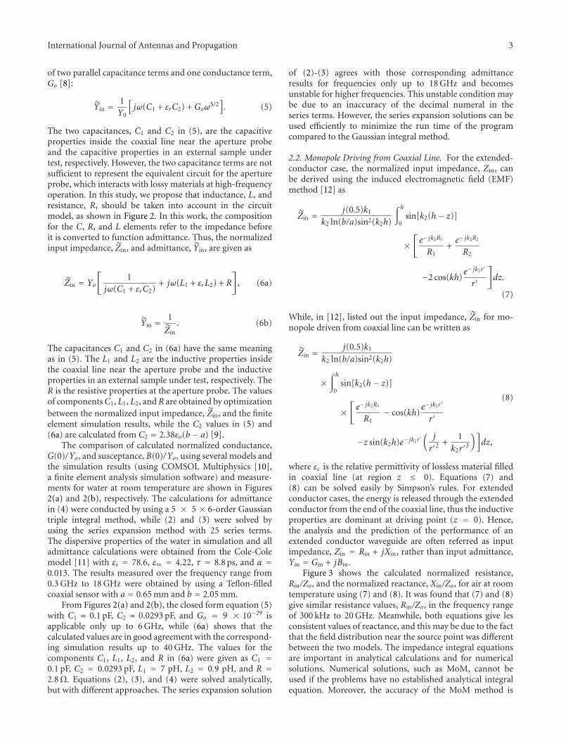
The two capacitances, C1 and C2 in (5), are the capacitiveproperties inside the coaxial line near the aperture probeand the capacitive properties in an external sample undertest, respectively. However, the two capacitance terms are notsufficient to represent the equivalent circuit for the apertureprobe, which interacts with lossy materials at high-frequencyoperation. In this study, we propose that inductance, L, andresistance, R, should be taken into account in the circuitmodel, as shown in Figure 2. In this work, the compositionfor the C, R, and L elements refer to the impedance beforeit is converted to function admittance. Thus, the normalizedinput impedance, Zin, and admittance, Yin, are given as

Zin = Yo

[1

jω(C1 + εrC2)+ jω(L1 + εrL2) + R

], (6a)

Yin = 1

Zin. (6b)

The capacitances C1 and C2 in (6a) have the same meaningas in (5). The L1 and L2 are the inductive properties insidethe coaxial line near the aperture probe and the inductiveproperties in an external sample under test, respectively. TheR is the resistive properties at the aperture probe. The valuesof componentsC1, L1, L2, andR are obtained by optimizationbetween the normalized input impedance, Zin, and the finiteelement simulation results, while the C2 values in (5) and(6a) are calculated from C2 = 2.38εo(b− a) [9].

The comparison of calculated normalized conductance,G(0)/Yo, and susceptance, B(0)/Yo, using several models andthe simulation results (using COMSOL Multiphysics [10],a finite element analysis simulation software) and measure-ments for water at room temperature are shown in Figures2(a) and 2(b), respectively. The calculations for admittancein (4) were conducted by using a 5 × 5 × 6-order Gaussiantriple integral method, while (2) and (3) were solved byusing the series expansion method with 25 series terms.The dispersive properties of the water in simulation and alladmittance calculations were obtained from the Cole-Colemodel [11] with εs = 78.6, ε∞ = 4.22, τ = 8.8 ps, and α =0.013. The results measured over the frequency range from0.3 GHz to 18 GHz were obtained by using a Teflon-filledcoaxial sensor with a = 0.65 mm and b = 2.05 mm.

From Figures 2(a) and 2(b), the closed form equation (5)with C1 = 0.1 pF, C2 = 0.0293 pF, and Go = 9 × 10−29 isapplicable only up to 6 GHz, while (6a) shows that thecalculated values are in good agreement with the correspond-ing simulation results up to 40 GHz. The values for thecomponents C1, L1, L2, and R in (6a) were given as C1 =0.1 pF, C2 = 0.0293 pF, L1 = 7 pH, L2 = 0.9 pH, and R =2.8Ω. Equations (2), (3), and (4) were solved analytically,but with different approaches. The series expansion solution

of (2)-(3) agrees with those corresponding admittanceresults for frequencies only up to 18 GHz and becomesunstable for higher frequencies. This unstable condition maybe due to an inaccuracy of the decimal numeral in theseries terms. However, the series expansion solutions can beused efficiently to minimize the run time of the programcompared to the Gaussian integral method.

2.2. Monopole Driving from Coaxial Line. For the extended-conductor case, the normalized input impedance, Zin, canbe derived using the induced electromagnetic field (EMF)method [12] as

Zin = j(0.5)k1

k2 ln(b/a)sin2(k2h)

∫ h

0sin[k2(h− z)]

×[e− jk2R1

R1+e− jk2R2

R2

−2 cos(kh)e− jk2r′

r′

]dz.

(7)

While, in [12], listed out the input impedance, Zin for mo-nopole driven from coaxial line can be written as

Zin = j(0.5)k1

k2 ln(b/a)sin2(k2h)

×∫ h

0sin[k2(h− z)]

×[e− jk2R1

R1− cos(kh)

e− jk2r′

r′

−z sin(k2h)e− jk2r′(

j

r′2+

1k2r′3

)]dz,

(8)

where εc is the relative permittivity of lossless material filledin coaxial line (at region z ≤ 0). Equations (7) and(8) can be solved easily by Simpson’s rules. For extendedconductor cases, the energy is released through the extendedconductor from the end of the coaxial line, thus the inductiveproperties are dominant at driving point (z = 0). Hence,the analysis and the prediction of the performance of anextended conductor waveguide are often referred as inputimpedance, Zin = Rin + jXin, rather than input admittance,Yin = Gin + jBin.

Figure 3 shows the calculated normalized resistance,Rin/Zo, and the normalized reactance, Xin/Zo, for air at roomtemperature using (7) and (8). It was found that (7) and (8)give similar resistance values, Rin/Zo, in the frequency rangeof 300 kHz to 20 GHz. Meanwhile, both equations give lesconsistent values of reactance, and this may be due to the factthat the field distribution near the source point was differentbetween the two models. The impedance integral equationsare important in analytical calculations and for numericalsolutions. Numerical solutions, such as MoM, cannot beused if the problems have no established analytical integralequation. Moreover, the accuracy of the MoM method is


COMSOL simulation

00

1

2

3

4

5

66.5

10 20 30 40

G(0

)/Yo

Frequency, f (GHz)

Equation (5)

Equation (6b)Equation (1)Equation (3)

Measured data

(a)

COMSOL simulation

0

0

1

2

3

4

10 20 30 40

4.5

−1.5

−1

B(0

)/Yo

Frequency, f (GHz)

Equation (5)

Equation (6b)Equation (1)Equation (4)

Measured data

(b)

Figure 2: Comparison of (a) normalized conductance, G(0)/Yo, and (b) normalized susceptance, B(0)/Yo, for water at 25◦C by consideringsize of probe with a = 0.65 mm and b = 2.05 mm.

Frequency, f (GHz)

0

1

2

3

4

5

6

7

8

Rin/Z

o

Equation (7)

Equation (8)

0 5 10 15 20

(a)

0 5 10 15 20

Frequency, f (GHz)

Equation (7)

Equation (8)

−10

−8

−6

−4

−2

0

2

4

6

7.5

Xin/Z

o

(b)

Figure 3: Comparison of calculated normalized resistance, Rin/Zo, and normalized reactance, Xin/Zo, for air at 25◦C using (7) and (8)(a = 0.65 mm, b = 2.05 mm, and h = 14.32 mm).

dependent on the rigor of the analytical integral equation.For instance, (1) and (8) have been used as the governingequations in the MoM method [7, 13, 14]. However, in theMoM solution, the current, Iz, is an unknown parameterthat must be solved by a numerical routine. Instead, inanalytical calculations, the current, Iz, is usually replacedby the sinusoidal current model [12, 13, 15] in the integralequation before it is solved.

The distribution current, Iz, substituted in (7) and (8)was assumed to have a convenient sinusoidal form, such as[12, 13, 15]:

Iz = I(0) sin k2(h− z)sin(k2h)

, (9)

where I(0) is the amplitude of the driving point current atz = 0, and it was canceled out in the derivations in (7) and


(8). Until now, no completely actual distribution current,Iz, formulation has existed for an arbitrarily sized extendedconductor. The current calculated using (9) is clearly the realvalue, but, in an actual case, the current is a complex valuedue to the azimuthal current, Iφ, contributed by the size ofthe radius of conductor a, as shown in Figure 4(b). Thismeans that (9) is valid only for thin extended conductors.In addition, it cannot be guaranteed that the currentdistribution will always be sinusoidal in all cases of theextended conductor.

Figure 5 shows the variational of distribution current, Izalong the length, z, of monopole. The unknown complexcurrent, Iz, is determined by using point matching MoM withPocklington’s integral equation and frill-generator source[14, 16, 17]. For cylindrical monopole structure, the mag-

netic field, �H , around the surface monopole which is gen-erated by a current, Iz, is in an azimuthal, φ, direction, andthe relationship is given as Hφ = Iz/2πaφ. This means thatthe imaginary part of current, Iz, is referring to the currentflow in z-direction (perpendicular to the φ direction). While,the real part of Iz is represented in the azimuthal current.From Figure 5, it is clear that, at low frequencies ( f <3 GHz), the value of current, Iz, is approaching the realnumber. When the monopole operated at higher frequencies,the distribution current, Iz, along the length of monopolebecome complex number.

In addition to the uncertainty of the distribution current,(7) and (8) also have not considered the fringing fieldscontributed by the electric field, Eρ, near the driving point(z = 0) and the end of the terminate conductor (z = h). Fora short conductor, (h < 10 a), driven from a coaxial line, theinput impedance is affected significantly by the fringing fieldat the end of the coaxial line, especially for high-frequencyoperation [18]. This means that the analytical impedanceformulas of (7) and (8) are accurate only for the low-frequency condition. For the reasons stated, the full wave(Hφ, Eρ, and Ez) analysis of the waveguide must be conductedby using a numerical method. In practice, the effects offringing fields at the driving point are always empiricallycorrected by capacitance, C f , element circuits.

In addition to integration models, the input impedanceof the monopole also can be represented by using thelumped-element model [19] and expressed as

Z = j(ωL1 − 1

ωC1

)︸︷︷︸

Low frequencies

+1

jωC2 +(1/(jωL2 + R1

))︸︷︷︸High frequencies

+1

jωC3 +[1/(jωL3 +

(50 jωL4/

(jωL4 + 50

)))]︸︷︷︸ .Driving fringing fields

(10)

From Figures 7(a) and 7(b), the input impedance showthat only two peaks of curve line occurred from 300 kHz to20 GHz, the three terms of (10) are sufficient to model theimpedance properties cover the frequency range. The firstterm in (10) describes the characteristics of the impedanceat low frequencies, while the second term contributes to the

modeling of impedance for high frequencies (>10 GHz). Thethird term is used to model the equivalent circuit, which isnear the driving point for the monopole. This means that ifthere are three peaks of impedance curve line (See Figure 14)over 300 kHz to 20 GHz, up to four terms of lumped-elementexpression are required. The equivalent circuit and all opti-mized values of resistance, R, capacitance, C, and inductance,L, elements in (10) for air are shown in Figure 6(b), and thevalues are accurate up to 20 GHz. The RLC values in (10)are obtained by optimizing (10) to the measurement results.At low frequencies, the capacitance term, C1, in (10) hasplayed an important role in the modeling, since the inputimpedance at driving point (z = 0) shows the natureof capacitive properties (Xin/Zo in negative (−) sign) at afrequency of less than 4 GHz, as shown in Figure 7(b).

For instance, a monopole with h = 1.436 cm driven fromthe coaxial line, as shown in Figure 6(a), was tested in thiswork. The comparison of calculated normalized resistance,Rin/Zo, and reactance, Xin/Zo, using several models, momentmethod [14, 16, 17], simulation results (using COMSOLMultiphysics [10] and CST Microwave Studio [20]), andmeasurements for air at room temperature are shown inFigures 7(a) and 7(b), respectively. Different from the coaxialprobe, for a monopole, the fringing field capacitance, C f ,elements first refer to the admittance before being convertedto the impedance function, as follows:

Y = 1Equation (7)

+ jωC f , (11a)

Zcorrected = 1

Y. (11b)

In this work, the value of C f was 5.5 pF. Figure 7 showsthat a 1.436 cm monopole has been matched with a standard,50Ω cable at a frequency of 4.6 GHz and 14.4 GHz.

2.3. Coupling Monopole Driving from Coaxial Line. Whentwo different lengths of monopoles are placed closed toeach other, as shown in Figure 8(a), the combination of twoelectromagnetic fields occurs. Now, the input impedance ofthe monopole is required to consider the self-radiation andmutual-radiation effects.

The mutual normalized impedance, Z12, is well expressedas [21]:

Z12 = j(0.5) k1

k2 ln(b/a) sin(k2h1) sin(k2h2)

×∫ h2

0sin[k2(h2 − z)]

×[e− jk 2 R′1

R′1+e− jk2R

′2

R′2

−2 cos(k2h1)e− jk2R′

R′

]dz,

(12)


Iz

(a)

Iz

Iφ

2a

(b)

Figure 4: (a) Ideal analytical line form current; (b) Actual situations of current distribution on a cylindrical extended conductor.

0 5 10 15

I z(m

A)

z (mm)

0.5 GHz

Re(Iz)

Im(Iz)

0.2

0.4

0.6

0.8

0.9

0

(a)

0 5 10 150

0.5

1

1.5

1.8

I z(m

A)

z (mm)

1 GHz

Re(Iz)

Im(Iz)

(b)

0 5 10 15

I z(m

A)

z (mm)

2 GHz

Re(Iz)

Im(Iz)

0

1

2

3

4

(c)

0 5 10 15

I z(m

A)

z (mm)

3 GHz

Re(Iz)

Im(Iz)

0

2

4

6

8

(d)

0 5 10 150

5

10

15

I z(m

A)

z (mm)

4 GHz

Re(Iz)

Im(Iz)

(e)

0

5

5 10

10

15

I z(m

A)

z (mm)

5 GHz

Re(Iz)

Im(Iz)

0

−7−5

14

(f)

Figure 5: Simulated distribution current, Iz, on the 1.436 cm of monopole driving from coaxial line with a = 0.65 mm and b = 2.05 mm.


L1 = 0.9 nH

L4 = 1.25 nH

C3 = 0.2 pFC2 = 0.55 pF

L3 = 1.15 nHC1 = 0.3 pF

b = 0.205 cm

L2 = 0.15 nH

z = 0

3.33Ω

50Ω

h =1.436 cmZo = 50Ω

2a = 0.13 cm

(a)

(b)

Figure 6: Dimensions of monopole and simulated electric fields contour; (b) equivalent circuit for input impedance of monopole at z = 0.

0 5 10 15 200

1

2

3

4

5

6

Frequency, f (GHz)

Rin/Z

o

CST resultsCOMSOL resultsMoment method

Equation (10)Equation (11b)Measured data

(a)

0 5 10 15 20

Frequency, f (GHz)

Xin/Z

o

CST resultsCOMSOL results

Moment method

Equation (10)Equation (11b)Measured data

−10

−8

−6

−4

−2

0

2

(b)

Figure 7: Comparison of (a) normalized resistance, Rin/Zo, and (b) normalized reactance, Xin/Zo, for air at 25◦C by considering size ofmonopole driving from coaxial line with a = 0.65 mm, b = 2.05 mm, and h = 14.32 mm.

where R′1 =√D2 + (z − h1)2, R′2 =

√D2 + (z + h1)2, and

R′ = √D2 + z2. Finally, the input impedance, Zin port-1, of

monopole 1 can be calculated as [15, 21, 22]:

Zin port-1 = Z11 − Z212

Z22, (13)

where the term Z11 = (7) is assumed to be equal to Z22, andZ21 is equal to Z12. Similarly, the input impedance, Zin port-1,

of the coupling monopole also can be represented by usingthe lumped-element model and expressed as

Zin port-1 = j(ωL1 − 1

ωC1

)︸︷︷︸

Low frequencies

+1

jωC2 +(1/(jωL2 + R1

))︸︷︷︸High frequencies

+1

jωC3 +[1/(jωL3 +

(50 jωL4/

(jωL4 + 50

)))]︸︷︷︸ .Driving fringing fields (14)


D

h1h2

−h1−h2

z = 0

Image

(a)

Excitationcoaxial port

D

Port-1 Port-2

2b

h

2a

(b)

Figure 8: (a) Arbitrary lengths of two parallel, mutually coupled monopoles; (b) actual configuration of coupling monopole with oneexcitation port.

50 Ω

C1 = 0.33 pF L1 = 0.7 nH L2 = 0.16 nH4Ω

C2 = 0.5 pF C3 = 0.225 pF

L3 = 1.2 nH

L4 = 1.25 nH

Figure 9: Equivalent circuit for input impedance of coupling monopole at port-1 (excitation port).

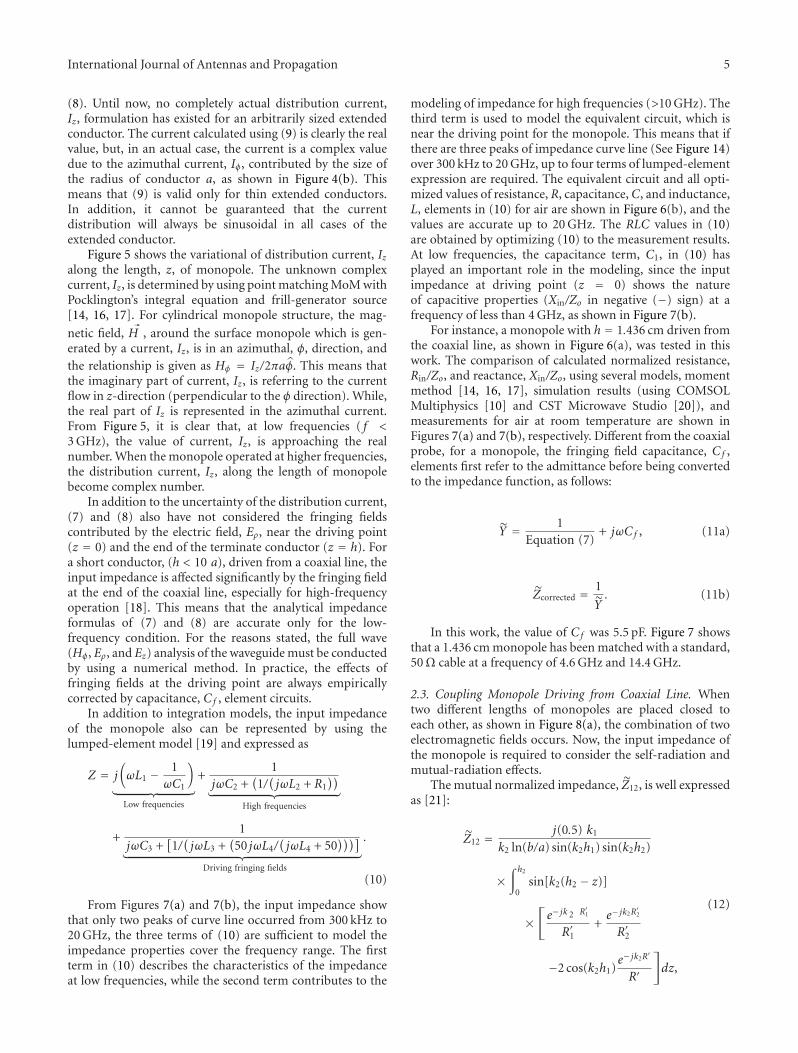
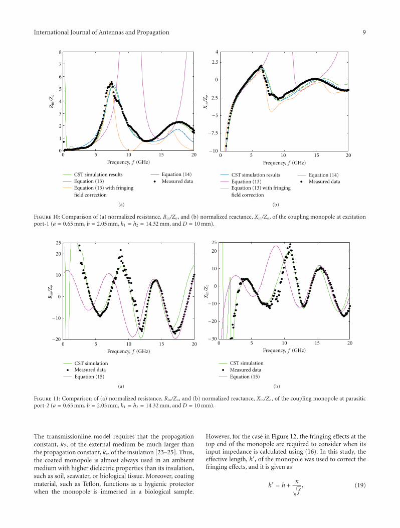
The equivalent circuit for (14) and its resistance, R,capacitance, C, and inductance, L, elements for air, whichare accurate up to 20 GHz, are shown in Figure 9. TheRLC values in equation (14) are obtained by optimizing(14) to the measurement results. From the comparisonof calculated normalized resistance, Rin/Zo, and reactance,Xin/Zo, using several models, the CST simulation results andmeasurements for air at room temperature are shown inFigures 10(a) and 10(b), respectively.

The equation for the coupling input impedance, Zin port-2,at port-2 can be expressed in terms of input impedance,Zin port-1, at excitation port-1 as

T =(

1− Equation (14)− Zo

Equation (14) + Zo

)e−(α+ jβ)d′ , (15a)

Zin port-2 = 2Zo

(1− T

T

), (15b)

where T is the transmission coefficient at parasitic port-2.The exponential term, e−(α+ jβ)d′ , is the transmission factor ofthe transmitted waves from port-1 to port-2. The symbolsα and β are the attenuation constant and phase constant,respectively. The equation d′ = h1 + h2 + D + Δ gives thelength of the transmission wave from port-1 to port-2. Thenormalized input impedances, Zin port-2 = Rin + jXin, calcu-lated by using (15b), are plotted and compared with mea-surement and CST simulation results, as shown in Figure 11.

The normalized resistance, Rin/Zo, and reactance, Xin/Zo, inFigures 11(a) and 11(b) are calculated with α = 3.18 ×10−5

√f neper/m, β = 2π f /c rad/m, d′ = 0.044 m and Zo =

50Ω.

2.4. Coated Conductor Driving from Coaxial Line. A coatedmonopole is a bare monopole enclosed by a thin cylindricallow-loss dielectric material with an outer radius, b, as shownin Figure 12.

In general, the transmission line formulas are adaptedeasily to the analysis of a coated antenna. The input impe-dance, Zin, of the coated monopole at the drive point (z = 0)[23–25] is expressed as

Zin = − jZc

Zocot(kLh′), (16)

where Zo and Zc are the characteristic impedance in thecoaxial line and the characteristic impedance for the coatedmonopole transmission line, respectively, which can be givenas:

Zc = γkL2πkc

[ln(b

a

)+(kck2

)2 H(2)o (k2b)

k2bH(2)1 (k2b)

]. (17)

The complex propagation constant, kL, is expressed as:

kL = kck2

[H(2)

o (k2b) + k2b ln(b/a)H(2)1 (k2b)

k2cH

(2)o (k2b) + k3

2b ln(b/a)H(2)1 (k2b)

]1/2

. (18)


Equation (13) with fringing

field correction

0 5 10 15 200

1

2

3

4

5

6

7

8

Frequency, f (GHz)

Rin/Z

o

CST simulation resultsEquation (13)

Equation (14)Measured data

(a)

Equation (13) with fringingfield correction

Frequency, f (GHz)

0 5 10 15 20−10

−7.5

−5

2.5

0

2.5

4

CST simulation resultsEquation (13)

Equation (14)Measured data

Xin/Z

o(b)

Figure 10: Comparison of (a) normalized resistance, Rin/Zo, and (b) normalized reactance, Xin/Zo, of the coupling monopole at excitationport-1 (a = 0.65 mm, b = 2.05 mm, h1 = h2 = 14.32 mm, and D = 10 mm).

0 5 10 15 20−20

−10

0

10

20

25

Frequency, f (GHz)

Rin/Z

o

CST simulationMeasured dataEquation (15)

(a)

CST simulationMeasured dataEquation (15)

0 5 10 15 20−30

−20

−10

0

10

20

25

Frequency, f (GHz)

Xin/Z

o

(b)

Figure 11: Comparison of (a) normalized resistance, Rin/Zo, and (b) normalized reactance, Xin/Zo, of the coupling monopole at parasiticport-2 (a = 0.65 mm, b = 2.05 mm, h1 = h2 = 14.32 mm, and D = 10 mm).

The transmissionline model requires that the propagationconstant, k2, of the external medium be much larger thanthe propagation constant, kc, of the insulation [23–25]. Thus,the coated monopole is almost always used in an ambientmedium with higher dielectric properties than its insulation,such as soil, seawater, or biological tissue. Moreover, coatingmaterial, such as Teflon, functions as a hygienic protectorwhen the monopole is immersed in a biological sample.

However, for the case in Figure 12, the fringing effects at thetop end of the monopole are required to consider when itsinput impedance is calculated using (16). In this study, theeffective length, h′, of the monopole was used to correct thefringing effects, and it is given as

h′ = h +κ√f

, (19)


z = 0

Coaxial line

Coated medium

k2

kc

2a

h

b

(a)

Hφ

Ground plane

(b)

Figure 12: (a) Two-dimensional and (b) three-dimensional configurations of a coated monopole.

0 5 10 15 200

1

2

3

4

4.5

Frequency, f (GHz)

Rin/Z

o

CST simulationCOMSOL simulationMeasured data

Equation (16)Equation (20)

Air

(a)

Air

0 5 10 15 20−4

−3

−2

−1

0

1

1.5

Frequency, f (GHz)

Xin/Z

o

CST simulationCOMSOL simulationMeasured data


(b)

Figure 13: Comparison of (a) normalized resistance, Rin/Zo, and (b) normalized reactance, Xin/Zo, for air at 25◦C by considering size ofprobe with a = 0.65 mm, c = 2.05 mm, and h = 13.92 mm.

where h and f are the actual length of the coated monopoleand the operational frequency, respectively. The symbol κ isa coefficient value which depends on the dimensions of themonopole. The fringing effects are assumed to be inverselyproportional to the square root of frequency. Similarly,the equivalent circuit can be used to represent the inputimpedance properties of the coated monopole, as shown inFigure 12, and the corresponding formulations are expressedas (20):

Zin = j(ωLT − 1

ωCT

)+

m∑n=1

[1

jωCn +(1/(jωLn + Rn

))]

+1

jωCB +[1/(jωLB +

(50 jωL′B/

(jωL′B + 50

)))] .(20)

Figures 13 and 14 show the calculated normalized resistance,Rin/Zo, and reactance, Xin/Zo, respectively, using several

Table 1: RCL component values in (20) for air and water samples.

RCL components Air Water

CB 0.33 pF 0.70 pF

CT 0.40 pF 2.50 pF

C1 0.54 pF 0.65 pF

C2 — 0.45 pF

LB 1 nH 1 nH

L′B 1.1 nH 2.4 nH

LT 0.5 nH 0.35 nH

L1 0.2 nH 0.32 nH

L2 — 0.16 nH

R1 2.9Ω 5.56Ω

R2 — 4.0Ω

models and the COMSOL simulation results and measure-ments for air and water at room temperature (25±1◦C) over


0 5 10 15 200

0.5

1

1.5

2

2.5

Frequency, f (GHz)

Rin/Z

o

COMSOL simulationMeasured data


Water

(a)

0 5 10 15 20−2

−1.5

−1

−0.5

0

0.5

1

Frequency, f (GHz)

COMSOL simulationMeasured data


Water

Xin/Z

o

(b)

Figure 14: Comparison of (a) normalized resistance, Rin/Zo, and (b) normalized reactance, Xin/Zo, for water at 25◦C by considering size ofprobe with a = 0.65 mm, c = 2.05 mm, and h = 13.92 mm.

the frequency range from 300 kHz to 20 GHz. The resultswere measured using a Teflon-coated monopole driven fromcoaxial line with a = 0.65 mm, c = 2.05 mm, and h =13.92 mm. The values for component resistor, R, reactor, L,and capacitor,C, in (20) for air and water are listed in Table 1,which provides the accurately calculated impedance up to20 GHz. The RLC values in (20) are obtained by optimizing(20) to the measurement results. As expected, comparedto the water sample, the calculated normalized resistance,Rin/Zo, and reactance, Xin/Zo, for air using (16) do notagree well with the measurements and simulation results.The propagation constant, γ, at the boundary between thecoated medium and the external medium is γ = ±ko√εr − εc,thus the tendency properties for the air case (k2 < kc) aredifferent those for the water case (k2 > kc). When k2 < kc, thewaves decay in the normal direction to the interface betweenthe coated dielectric and external medium due to the fact thatthe corresponding propagation constant, γ, is imaginary.

3. Conclusions

In this work, the coaxial waveguide was used as an example ofthe problem of linking electromagnetic theory with practicalmodeling, since the coaxial slot waveguides have been usedas antennas over the past of 70 years. Recently, manyscientific applications have involved this kind of waveguide.For instance, an open-ended coaxial probe was applied asa dielectric probe to measure the dielectric properties ofthe material being tested. In addition, the dielectric-coatedmonopole was used for hyperthermia treatment, and thecoupler monopole was designed to be an array antenna.Hence, many models have been developed for the coaxialwaveguide, and those models have been modified for use inmodeling other devices. In particular, the sinusoidal current

model is also used for planar waveguides. In this study,the accuracy of frequency-domain analytical models wastested by acquiring measurements and numerical simulationresults. We found that the semiempirical equivalent circuitmodeling worked successfully, covered a wide frequencyrange, and was very useful in the design of circuits thatmatched the waveguides. Although the analytical modelsare less accurate compare to numerical method, it providessignificant rapid and economize computation. Implicitly, theanalytical models still retain the academy valuable, especiallyfor who has preliminary study of the antenna modeling.

Acknowledgment

This study was supported by the Fundamental ResearchGrant Scheme (FRGS) Phase 2/2009 from Ministry of HigherEducation Malaysia under Project nD. 78486.

References

[1] K. S. Yee, “Numerical solution of initial boundary value prob-lems involving Maxwell’s equations in isotropic media,” IEEETransactions on Antennas and Propagation, vol. 14, pp. 302–307, 1966.

[2] R. F. Harrington, “Matrix methods for field problems,” Pro-ceedings of the IEEE, vol. 55, pp. 136–149, 1967.

[3] P. P. Silvester, “Finite element solution of homogeneous wave-guide problems,” Alta Frequenza, vol. 38, pp. 313–317, 1969.

[4] H. Levine and C. H. Papas, “Theory of the circular diffractionantenna,” Journal of Applied Physics, vol. 22, no. 1, pp. 29–43,1951.

[5] N. Marcuvitz, Waveguide Handbook, Boston Technical Pub-lishers, Boston, Mass, USA, 1964.

[6] D. K. Misra, “A quasi-static analysis of open-ended coaxiallines,” IEEE Transactions on Microwave Theory and Techniques,vol. 35, no. 10, pp. 925–928, 1988.


[7] R. D. Nevels, C. M. Butler, and W. Yablon, “The annular slotantenna in a lossy biological medium,” IEEE Transactions onMicrowave Theory and Techniques, vol. 33, no. 4, pp. 314–319,1985.

[8] M. A. Stuchly, M. M. Brady, S. S. Stuchly, and G. Gajda,“Equivalent circuit of an open-ended coaxial line in a lossydielectric,” IEEE Transactions on Instrumentation and Measure-ment, vol. 31, no. 2, pp. 116–119, 1982.

[9] G. B. Gajda and S. S. Stuchly, “Numerical analysis of open-ended coaxial lines,” IEEE Transactions on Microwave Theoryand Techniques, vol. 31, no. 5, pp. 380–384, 1983.

[10] COMSOL Multiphysics, “RF module model library version3.5a,” COMSOL AB, TegnZrgatan, Sweden, 2008.

[11] A. Nyshadham, C. L. Sibbald, and S. S. Stuchly, “Permittivitymeasurements using open-ended sensors and reference liquidcalibration—an uncertainty analysis,” IEEE Transactions onMicrowave Theory and Techniques, vol. 40, no. 2, pp. 305–314,1992.

[12] M. M. Weiner, S. P. Cruze, C. C. Li, and W. J. Wilson, MonopoleElements on Circular Ground Plane, Artech House, New York,NY, USA, 1987.

[13] D. K. Misra, “A study on coaxial line excited monopole probesfor In-Situ permittivity measurements,” IEEE Transactions onInstrumentation and Measurement, vol. 30, pp. 46–51, 1987.

[14] C. A. Balanis, Advanced Engineering Electromagnetic, JohnWiley & Sons, New York, NY, USA, 1989.

[15] R. W. P. King, R. B. Mack, and S. Sandler, Arrays of CylindricalDipoles, Cambridge University Press, Cambridge, UK, 1968.

[16] W. C. Gibson, The Method of Moments in Electromagnetics,Chapman & Hall/CRC, London, UK, 2008.

[17] R. Garg, Analytical and Computational Methods in Electromag-netics, Artech House, Norwood, Mass, USA, 2008.

[18] K. Y. You, Z. Abbas, K. Khalid, and N. F. Kong, “Improved for-mulation for admittance of thin and short monopole drivingfrom coaxial line into dissipative media,” IEEE Antennas andWireless Propagation Letters, vol. 8, pp. 1246–1249, 2009.

[19] B. S. Yarman, Design of Ultra Wideband Antenna MatchingNetworks, Springer, Berlin, Germany, 2008.

[20] CST Microwave Studio, “CST Microwave Studio—Workflow& Solver Overview,” CST Computer Simulation Technology,Darmstadt, Germany, 2008.

[21] R. E. Collin, Antennas and Radiowave Propagation, McGraw-Hill, New York, NY, USA, 1985.

[22] E. E. Altshuler, “Self- and mutual impedances of traveling-wave linear antennas,” IEEE Transactions on Antennas andPropagation, vol. 37, no. 10, pp. 1312–1316, 1989.

[23] L. Kuan Min, “Chapter 11: insulated linear antenn,” in Re-search Topics in Electromagnetic Wave Theory, J. A. Kong, Ed.,John Wiley & Sons, New York, NY, USA, 1967.

[24] R. W. P. King, S. R. Mishra, K. M. Lee, and G. S. Smith, “Theinsulated monopole: admittance and junction effects,” IEEETransactions on Antennas and Propagation, vol. 23, no. 2, pp.172–177, 1975.

[25] T. W. Hertel and G. S. Smith, “The insulated linear antenna-revisited,” IEEE Transactions on Antennas and Propagation, vol.48, no. 6, pp. 914–920, 2000.

International Journal of

AerospaceEngineeringHindawi Publishing Corporationhttp://www.hindawi.com Volume 2010

RoboticsJournal of

Hindawi Publishing Corporationhttp://www.hindawi.com Volume 2014


Active and Passive Electronic Components

Control Scienceand Engineering

Journal of



RotatingMachinery


Hindawi Publishing Corporation http://www.hindawi.com

Journal ofEngineeringVolume 2014

Submit your manuscripts athttp://www.hindawi.com

VLSI Design



Shock and Vibration


Civil EngineeringAdvances in

Acoustics and VibrationAdvances in



Electrical and Computer Engineering

Journal of

Advances inOptoElectronics

Hindawi Publishing Corporation http://www.hindawi.com

Volume 2014

The Scientific World JournalHindawi Publishing Corporation http://www.hindawi.com Volume 2014

SensorsJournal of


Modelling & Simulation in EngineeringHindawi Publishing Corporation http://www.hindawi.com Volume 2014


Chemical EngineeringInternational Journal of Antennas and

Propagation




Navigation and Observation



DistributedSensor Networks


Review Article - Hindawi Publishing Corporationdownloads.hindawi.com/journals/ijap/2012/701532.pdfFor instance, many online broad-band dielectric measurements involve the prediction

Documents