Review 3D Deep Learning on Medical Images: A Review

Review

3D Deep Learning on Medical Images: A Review

Satya P. Singh 1,2, Lipo Wang 3, Sukrit Gupta 4, Haveesh Goli 4, Parasuraman Padmanabhan 1,2,*

and Balázs Gulyás 1,2,5

1 Lee Kong Chian School of Medicine, Nanyang Technological University Singapore, 608232, Singapore;

[email protected] (S.P.S.); [email protected] (B.G.) 2 Cognitive Neuroimaging Centre, Nanyang Technological University Singapore, 636921, Singapore 3 School of Electrical and Electronic Engineering, Nanyang Technological University Singapore, 639798,

Singapore; [email protected] 4 School of Computer Science and Engineering, Nanyang Technological University Singapore, 639798,

Singapore; [email protected] (S.G.); [email protected] (H.G.) 5 Department of Clinical Neuroscience, Karolinska Institute, 17176 Stockholm, Sweden

* Correspondence: [email protected]

Received: 10 July 2020; Accepted: 3 September 2020; Published: date

Abstract: The rapid advancements in machine learning, graphics processing technologies and the

availability of medical imaging data have led to a rapid increase in the use of deep learning models

in the medical domain. This was exacerbated by the rapid advancements in convolutional neural

network (CNN) based architectures, which were adopted by the medical imaging community to

assist clinicians in disease diagnosis. Since the grand success of AlexNet in 2012, CNNs have been

increasingly used in medical image analysis to improve the efficiency of human clinicians. In recent

years, three-dimensional (3D) CNNs have been employed for the analysis of medical images. In

this paper, we trace the history of how the 3D CNN was developed from its machine learning roots,

we provide a brief mathematical description of 3D CNN and provide the preprocessing steps

required for medical images before feeding them to 3D CNNs. We review the significant research

in the field of 3D medical imaging analysis using 3D CNNs (and its variants) in different medical

areas such as classification, segmentation, detection and localization. We conclude by discussing

the challenges associated with the use of 3D CNNs in the medical imaging domain (and the use of

deep learning models in general) and possible future trends in the field.

Keywords: 3D convolutional neural networks; 3D medical images; classification; segmentation;

detection; localization.

1. Introduction

Medical images have varied characteristics depending on the target organ and the suspected

diagnosis. Common modalities used for medical imaging include X-ray, computed tomography

(CT), diffusion tensor imaging (DTI), positron emission tomography (PET), magnetic resonance

imaging (MRI), and functional MRI (fMRI) [1–4]. In the past thirty years, these radiological image

acquisition technologies have enormously improved in terms of acquisition time, image quality,

resolution [5–8] and have become more affordable. Despite improvements in hardware, all

radiological images require subsequent image analysis and diagnosis by trained human radiologists

[9]. Besides the significant time and economic costs involved in training radiologists, radiologists

also suffer from limitations due to their lack of experience, time and fatigue. This becomes especially

significant because of an increasing number of radiological images due to the aging population and

more prevalent scanning technologies that put additional stress on radiologists [9–12]. This puts a

focus on automated machine learning algorithms that can play a crucial role in assisting clinicians in

alleviating their onerous workloads.

Deep learning refers to learning patterns in data samples using neural networks containing

multiple interconnected layers of artificial neurons [11]. An artificial neuron by analogy to a

biological neuron is something that takes multiple inputs, performs a simple computation and

produces an output. This simple computation has the form of a linear function of the inputs

followed by an activation function (usually non-linear). Examples of some commonly used

non-linear activation functions are the hyperbolic tangent (tanh), sigmoid transformation and the

rectified linear unit (ReLU) and their variants [13]. The development of deep learning can be traced

back to Walter Pitts and Warren McCulloch (1943). Their work has been followed by significant

advancements due to the development of the backpropagation model (1960), convolutional neural

networks (CNN) (1979), long short-term memory (LSTM) (1997), ImageNet (2009) and AlexNet

(2011) [14]. In 2014, Google presented GoogLeNet (Winner of ILSVRC 2014 challenge) [15], which

introduced the concept of inception modules that drastically reduced the computational complexity

of CNN. Deep learning is essentially a reincarnation of the artificial neural network where we stack

layer upon layer of artificial neurons. Using the outputs of the terminal layers built on the outputs of

previous layers, we can start to describe arbitrarily complex patterns. In the CNN [14], network

features are generated by convolving kernels in a layer with outputs of the previous layers, such that

the first hidden layer kernels perform convolutions on the input images. While the features captured

by early hidden layers are generally shapes, curves or edges, deeper hidden layers capture more

abstract and complex features.

Historical methods for automated classification of images involves extensive rule-based

algorithms or manual feature handcrafting [16–21], which are time-consuming, have poor

generalization capacity and require domain knowledge. All this changed with the advent and

demonstrated the success of CNNs. CNNs are devoid of any manual feature handcrafting, require

little preprocessing and are translation-invariant [22]. In CNNs, low-level image features are

extracted by the initial layers of filters and progressively higher features are learnt by successive

layers before classification. The commonly seen X-ray is an example of a two-dimensional (2D)

medical image. The machine learning of these medical images is no different from CNNs applied to

classify natural images in recent years, e.g., the ImageNet Large Scale Visual Recognition

Competition [14]. With decreasing computational costs and powerful graphics processing (units

(GPUs) available, it has become possible to analyze three-dimensional (3D) medical images, such as

CT, DTI, fMRI, Ultrasound and MRI scans [14] using 3D deep learning. These scans give detailed

three-dimensional images of human organs and can be used to detect infection, cancers, traumatic

injuries and abnormalities in blood vessels and organs. The major drawback in the application of 3D

deep learning on medical images is the limited availability of data and high computational cost.

Further, there is a problem of the curse of dimensionality. However, with the recent advancements

in neural network architectures, data augmentation techniques and high-end GPUs, it is becoming

possible to analyze the volumetric medical data using 3D deep learning. Consequently, since 2012,

we have seen exponential growth in the applications of 3D deep learning in different medical image

modalities. Here, we present a systematic review of the applications of 3D deep learning in medical

imaging with possible future directions. To the best of our knowledge, this is the first review paper

of 3D deep learning on medical images.

2. Materials and Methods

In a very short time, deep learning techniques have become an alternative to many machine

learning algorithms that were traditionally used in medical imaging. We explored various terms

used in medical imaging literature to understand the trend in using deep learning in medical

imaging applications. We searched for ‘machine learning + medical’ in the title and abstract in

PubMed publication database (on 9 July 2020) and across a predictable trend of using more and

more similar data in different approaches (Figure 1). We observed a similar trend for the query ‘deep

learning + medical’, albeit with few publications before 2015. However, while searching for the

query ‘3D deep learning + medical’ in the title and abstract, we see a different scenario. An

exponential increase can be seen for ‘deep learning’ and ‘3D deep learning’ after 2015 and 2017

onwards, respectively. This signifies that, while there was not much work in the domain a few years

ago, there has been an accelerated rise in the number of publications related to deep learning for

both 2D and 3D images.

Figure 1. Year-wise number of publications in PubMed while searching for ‘deep learning + medical’

and ‘3D deep learning + medical’ in the title and abstract in PubMed publication database (as at 1st

July 2020).

In this systematic review, we searched for the applications of 3D deep learning in medical

image segmentation, classification, detection and localization. For the literature search, we chose

three database platforms, namely Google Scholar, PubMed and Scopus. The application of 3D CNN

effectively came into the picture after the remarkable success of AlexNet in 2012, which was enabled

by advanced parallel computing architecture. Between 2015 and 2016, we have seen exponential

growth in the literature related to 3D deep learning in medical imaging, and therefore, we limited

our search to after 1 January 2012. The first search was performed on 12 September 2019, and the

second search on 1 January 2020, while the third search was performed on 1 July 2020. The literature

search and selection for the study were done according to the preferred reporting items for

systematic seviews and meta-analyses (PRISMA) statement [23]. We searched for title and abstract

with different keyword combination of “3D CNN”, “medical imaging”, “classification”,

“segmentation”, “detection” and “localization” and selected 31,576 records. 11,987 duplicate records

Figure 2. Criteria for literature selection for systematic review according to preferred reporting items

for systematic reviews and meta-analyses (PRISMA) [23] guidelines.

were removed. After studying the title and abstract, we further removed 19,380 records. We further

excluded 77 records. Finally, we collected 132 papers for our review purpose. The details about the

inclusion and exclusion of papers according to the PRISMA statement is depicted in Figure 2.

2.1. A Typical Architecture of 3D CNN

A typical architecture of CNN may include four basic components: (1) local receptive field, (2)

sharing weights, (3) pooling and (4) fully connected (fc) layers. Deep CNN architecture is

constructed by stacking several convolutional layers and pooling layers and one or so fully

connected layers at the end of the network [9,24]. While 1D CNN can extract spectral features from

the data, 2D CNN can extract spatial features from the input data. However, 3D CNNs can take

advantage of both 1D and 2D CNNs by extracting both spectral and spatial features simultaneously

from the input volume. These 3D CNN features are very useful in analyzing the volumetric data in

medical imaging. The mathematical formulation of 3D CNN is very similar to 2D CNN with an extra

dimension added. The basic architecture of 3D CNN is shown in Figure 3. We briefly discuss the

mathematical background of 3D CNN.

Figure 3. Typical architecture of 3D CNN.

Convolutional Layer: The basic definition, principle, and working equation of 3D CNN is quite

similar to 2D CNN. We only add an extra dimension of depth to the working equation of 2D CNN.

Suppose 3D CNN of input 𝑥 has a dimension of 𝑀 × 𝑁 × 𝐷 with 𝑖, 𝑗, 𝑘 as iterators. The kernel 𝜔

with dimensions 𝑛1 × 𝑛2 × 𝑛3 has iterator 𝑎, 𝑏, 𝑐. We denote ℓ is the ℓ𝑡ℎ, where ℓ = 1 is the first

layer and ℓ = 𝐿 is the last layer. We denote 𝑦ℓ and 𝑏ℓ as the output and the bias unit the ℓ𝑡h layer.

To compute the nonlinear input 𝑥𝑖,𝑗,𝑘ℓ to (𝑖, 𝑗, 𝑘)𝑡ℎ unit in layer ℓ , we add up the weight

contribution from the previous layer as follows:

𝑥𝑖,𝑗,𝑘ℓ = ∑ ∑ ∑ 𝜔𝑎,𝑏,𝑐𝑦(𝑖+𝑎)(𝑗+𝑏)(𝑘+𝑐)

ℓ−1 + 𝑏ℓ𝑐𝑏𝑎 . (1)

The output of the (𝑖, 𝑗)𝑡ℎ unit in the ′ℓ𝑡ℎ′ convolutional layer is given as follows:

𝑦𝑖,𝑗,𝑘ℓ = 𝑓(𝑥𝑖,𝑗,𝑘

ℓ ). (2)

Pooling Layer: Each feature map in the convolutional layer of 3D CNN can be a pooling layer.

There are two kinds of pooling. If the pooling layer averages across the group of input voxels, it is

called average pooling, while if it obtains a maximum of the input voxels, it is called maximum

pooling. The output of the pooling layer will be the input of the next layer. Since a small shift in the

input image results in a shift in activation function, the pooling layer also introduces some

translational invariance to the 3D CNN. To lower the sampling effect of pooling, we can remove the

pooling layer by increasing the number of strides in the preceding CNN layer [25]. This will not

result in any significant depreciation of the performance. However, by doing this, we significantly

Convolution

Subsampling

Convolution

Convolution

Flatten Output

3D Input Feature Extraction Classification

Subsampling

reduce the overlap in the CNN layer that precedes the pooling layer. This is simply equivalent to the

pooling operation where only the top-left features are considered.

Dropout regularization: Deep neural networks with a large number of parameters are very

dominant learning systems. Multiple deep nonlinear hidden layers allow them to learn complex

relationships between input and outputs. However, with the limited training data, these complex

relationships introduce sampling noise, which appears in training data sets but not in real test

datasets even if both are drawn from the same distribution. This scenario leads to overfitting and

there have been several strategies [26] to tackle the problem, such as early stopping of the training

epochs and weight penalties (L1 and L2 regularizations, soft weight sharing, and pooling). Ensemble

models of several CNNs with different configurations on the same dataset are known for their

overfitting. However, this leads to extra computational and maintenance cost for training several

models. Moreover, training a large network requires large datasets, but the availability of such

datasets in the field of medical imaging is very rare. Even if one can train large networks with a

versatile setting of parameters, testing these networks is not feasible in a real-time situation due to

the nature of medical imaging systems. In the case of ensemble models, a CNN model can also

simulate multiple configurations just by probabilistically dropping out edges and nodes. Dropout is

a kind of regularization technique to reduce overfitting by temporarily dropping a unit out of the

network [27]. This simple idea shows a significant improvement in CNN performance.

Batch normalization: The input of each hidden layer dynamically changes during training

because the parameters in the previous layer update at each training epoch. If these changes are

large, the search for an optimal hyperparameter becomes difficult for the network and may be

computationally expensive to reach an optimal value. This problem can be solved by an algorithm

called batch normalization, which was proposed by two researchers [28]. Batch normalization allows

the use of a higher learning rate and thereby achieves the optimal value in less time. It facilitates the

smooth training of deeper network architectures in less time. The normalization of data from a

particular batch is about finding the mean and variance of the data points from mini-batch and

normalizing them to have a zero mean and unit variance.

In backward pass, the CNN adjusts its weights and parameters according to the output by

calculating the error through some loss functions, 𝑒 (other names are cost function and error

function) and backpropagating the error with some rules towards the input. The loss is calculated by

taking the partial derivative of 𝑒 w.r.t., which is the output of each neuron in that layer, such as

𝜕𝑒/𝑦𝑖,𝑗,𝑘ℓ for the output, 𝑦𝑖,𝑗,𝑘

ℓ of (𝑖, 𝑗, 𝑘)𝑡ℎ unit in layer ℓ. The cFhain rule allows us to write and add

up the contribution of each variable as follows:

𝜕𝑒

𝜕𝑥𝑖,𝑗,𝑘ℓ =

𝜕𝑒

𝜕𝑦𝑖,𝑗,𝑘ℓ

𝜕𝑓(𝑦𝑖,𝑗,𝑘ℓ )

𝜕𝑥𝑖,𝑗,𝑘ℓ =

𝜕𝑒

𝜕𝑦𝑖,𝑗,𝑘ℓ 𝑓′(𝑥𝑖,𝑗,𝑘

ℓ )#. (3)

Weights in the previous convolutional layer can be updated by backpropagating the error to the

previous layer according to the following equation:

𝜕𝑒

𝜕𝑦𝑖,𝑗,𝑘ℓ−1

= ∑ ∑ ∑𝜕𝑒

𝜕𝑥(𝑖−𝑎),(𝑗−𝑏),(𝑘−𝑐)ℓ

𝑛3−1

𝑐=0

𝑛2−1

𝑏=0

𝜕𝑥(𝑖−𝑎),(𝑗−𝑏),(𝑗−𝑏)ℓ

𝜕𝑦𝑖,𝑗,𝑘ℓ−1

𝑛1−1

𝑎=0

. (4)

= ∑ ∑ ∑𝜕𝑒

𝜕𝑥(𝑖−𝑎),(𝑗−𝑏),(𝑘−𝑐)ℓ

𝑛3−1𝑏=0

𝑛2−1𝑎=0 𝜔𝑎,𝑏,𝑐

𝑛1−1𝑎=0 . (5)

Equation (5) allows us to calculate the error for the previous layer. Further, the above eq. makes

sense for those points which are n times away from each side of the input data. This situation can be

avoided by simply padding with zeros to the end of each side of the input volume.

2.2. Breakthroughs in CNN Architectural Advances

Several different versions of CNN have been proposed in the literature to improve model

performance. In 2011, Krizhevsky et al. [14] presented a deep CNN architecture. A systematic

architecture of AlexNet is shown in Figure 4. AlexNet has five convolutional layers and three fully

connected layers (the last FC layer was the SoftMax layer). The network was trained on 1.2 million

images with 60 million parameters. To tackle these large parameters, AlexNet was trained on a

multi-GPU (2-GPUs, 3GB GTX-580) environment by systematically distributing the neurons on both

the GPUs. Data augmentation and dropouts were used to avoid overfitting. Data augmentation was

done in two ways: (1) image translations and horizontal reflections, and (2) changing the intensity of

RGB channels. The AlexNet architecture has won ILSVRC-2012 (ImageNet Large Scale Visual

Recognition Competition-2012) with a large margin. The difference between the top-five test errors

of AlexNet (15.3%) and the second prize winner (26.2%) was around 10%.

Figure 4. A typical architecture of AlexNet [14].

In 2014, Simonyan and Zisserman [29] presented a more profound deep network architecture

called VGGNet (Visual Geometry Group Network) (16 layers and 19 layers) for the ImageNet

Challenge 2014 and secured the first position for the localization task and the second position for the

classification task. VGGNet uses 3 × 3 filters for convolutional layers and three consecutive fully

connected layers 4096, 4096, and 1000 in size, respectively. The design of VGGNet is quite similar to

AlexNet. Adding consecutive layers to the network increases the number of parameters that cause

networks to suffer from errors and overfitting. In supervising learning, the deeper network requires

large data for training and despite the use of data augmentation techniques, it may happen that the

data is not sufficient. Further, annotating such a large amount of data can be quite expensive.

Furthermore, because a linear increase in the filter emerges as a result of a quadratic increase in

computational burden, deeper networks lead us to a computational explosion. In deeper layers,

weights can be near zero and emerge as a waste of computational resources. Fast forwarding from

2012, in 2014, the designers at Google presented the concept of “Inception” based on the Hebbian

principle and the intuition of multiple-scale processing, and the network was called GoogLeNet

(also known as Inception-V1) [15]. The intuition behind the inception module (version V1) (Figure

5a) is that the optimal neural network topology can be built by clustering neurons to the correlation

statistics in the input images. The authors analyzed the correlation statistics in the activations in the

previous layer and clustered the neurons with highly correlated outputs for the next layer. In the

images, the correlation tends to be local, and therefore, performing convolutions over the local

patches can cluster the neurons. In lower layers, there exists a high correlation between local pixels

in a surrounding patch. These pixels can be covered by a small 1 × 1 convolution. Besides, the

correlation between a smaller number of spatially spread-out clusters can be quantified by 3 × 3 and

5 × 5 convolutions. In order take effect of 1 × 1, 3 × 3 and 5 × 5, the authors stacked them as a single

output vector for the next layer (Figure 5a). In addition, to take the advantages of maximum

(max)-pooling, they also concatenated a pooling layer in parallel (3 × 3 max pooling branch in Figure

22

7

227

11

11

55 327

27 3

3

3

33

33

192

11

11

128

192 128

Max

po

olin

g

Max

po

olin

g

Max

po

olin

g D

en

se

De

nse

20

48

20

48

10

00

55

13 13

13

Input

Conv 1 Conv 2 Conv 3 Conv 5Conv 4

10

00

-way

So

ftM

ax

55 327

27 3

3

3 5

20

48

20

48

Dropout

Inter-GPU connections

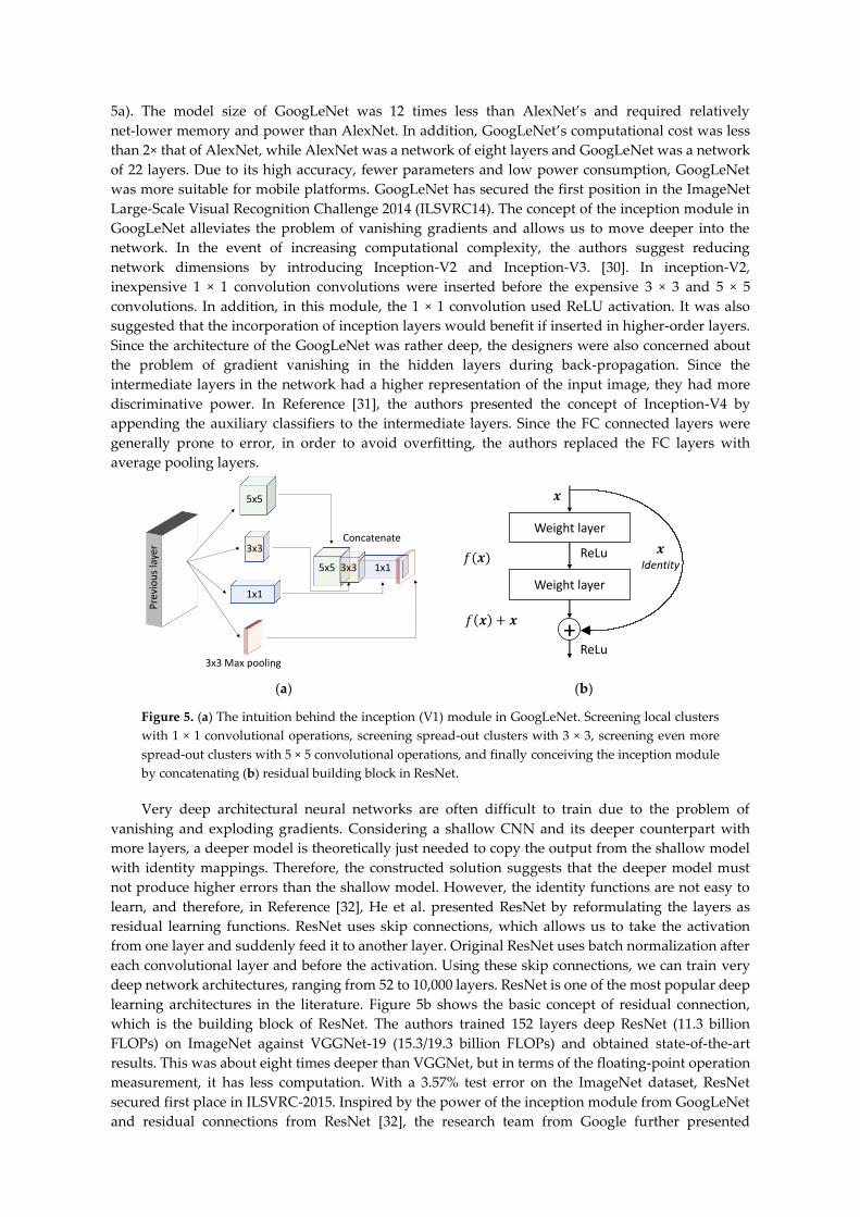
5a). The model size of GoogLeNet was 12 times less than AlexNet’s and required relatively

net-lower memory and power than AlexNet. In addition, GoogLeNet’s computational cost was less

than 2× that of AlexNet, while AlexNet was a network of eight layers and GoogLeNet was a network

of 22 layers. Due to its high accuracy, fewer parameters and low power consumption, GoogLeNet

was more suitable for mobile platforms. GoogLeNet has secured the first position in the ImageNet

Large-Scale Visual Recognition Challenge 2014 (ILSVRC14). The concept of the inception module in

GoogLeNet alleviates the problem of vanishing gradients and allows us to move deeper into the

network. In the event of increasing computational complexity, the authors suggest reducing

network dimensions by introducing Inception-V2 and Inception-V3. [30]. In inception-V2,

inexpensive 1 × 1 convolution convolutions were inserted before the expensive 3 × 3 and 5 × 5

convolutions. In addition, in this module, the 1 × 1 convolution used ReLU activation. It was also

suggested that the incorporation of inception layers would benefit if inserted in higher-order layers.

Since the architecture of the GoogLeNet was rather deep, the designers were also concerned about

the problem of gradient vanishing in the hidden layers during back-propagation. Since the

intermediate layers in the network had a higher representation of the input image, they had more

discriminative power. In Reference [31], the authors presented the concept of Inception-V4 by

appending the auxiliary classifiers to the intermediate layers. Since the FC connected layers were

generally prone to error, in order to avoid overfitting, the authors replaced the FC layers with

average pooling layers.

(a) (b)

Figure 5. (a) The intuition behind the inception (V1) module in GoogLeNet. Screening local clusters

with 1 × 1 convolutional operations, screening spread-out clusters with 3 × 3, screening even more

spread-out clusters with 5 × 5 convolutional operations, and finally conceiving the inception module

by concatenating (b) residual building block in ResNet.

Very deep architectural neural networks are often difficult to train due to the problem of

vanishing and exploding gradients. Considering a shallow CNN and its deeper counterpart with

more layers, a deeper model is theoretically just needed to copy the output from the shallow model

with identity mappings. Therefore, the constructed solution suggests that the deeper model must

not produce higher errors than the shallow model. However, the identity functions are not easy to

learn, and therefore, in Reference [32], He et al. presented ResNet by reformulating the layers as

residual learning functions. ResNet uses skip connections, which allows us to take the activation

from one layer and suddenly feed it to another layer. Original ResNet uses batch normalization after

each convolutional layer and before the activation. Using these skip connections, we can train very

deep network architectures, ranging from 52 to 10,000 layers. ResNet is one of the most popular deep

learning architectures in the literature. Figure 5b shows the basic concept of residual connection,

which is the building block of ResNet. The authors trained 152 layers deep ResNet (11.3 billion

FLOPs) on ImageNet against VGGNet-19 (15.3/19.3 billion FLOPs) and obtained state-of-the-art

results. This was about eight times deeper than VGGNet, but in terms of the floating-point operation

measurement, it has less computation. With a 3.57% test error on the ImageNet dataset, ResNet

secured first place in ILSVRC-2015. Inspired by the power of the inception module from GoogLeNet

and residual connections from ResNet [32], the research team from Google further presented

5x5

1x1

3x3

5x5 1x13x3

Concatenate

Pre

vio

us

laye

r

3x3 Max pooling

Fig conceiving the inception module

Inception-ResNet [31]. They showed that the residual connections accelerate training in the

inception network and thereby improved the performance of the Inception network. Continuous

concatenation of convolutional layers on the top of activations will make the training worse.

Ronneberger et al. [33] proposed U-Net, which was the winner of the ISBI cell tracking challenge

2015 for biomedical image segmentation tasks. U-Net can be trained with a relatively small number

of samples and achieves high accuracy in a short time. U-Net involves the symmetrical expansion

and contraction paths with skip connections. In 2016, Cicek et al. [34] presented a modified version

of the original U-Net i.e., 3D U-Net for volumetric segmentation from sparse notation.

3. 3D Medical Imaging Pre-Processing

Preprocessing of the image dataset before feeding the CNN or other classifiers is important for

all types of imaging modalities. Several preprocessing steps are recommended for the medical

images before they are fed as input to the deep neural network model, such as (1) artifact removal,

(2) normalization, (3) slice timing correction (STC), (4) image registration and (5) bias field

correction. While all the steps, (1) to (5), help in getting reliable results, STC and image registration

are very important in the case of 3D medical images (especially MR and CT images). Artifact

removal and normalization are the most performed preprocessing steps across the modalities. We

briefly discuss pre-processing steps above.

The first part of any preprocessing pipeline is the removal of artifacts. For example, we may be

interested in removing skulls in brain CT scans before feeding to 3D CNN. Removal of extracerebral

tissues is highly recommended before analyzing the T1 or T2 weighted MRI, and DTI modalities for

brain images. fMRI data often contains transient spike artifacts or a slowed over drift time. Thus, the

principal component analysis technique can be used to look at these spike related artifacts [3,35,36].

Before feeding the data for preprocessing to an automated pipeline, a manual check is also

advisable. For example, if the input T1 anatomical data is large, the FSL’s BET command will not

perform proper brain region extraction, and if we use images with artifacts for the popular fMRI

preprocessing tool fMRIprep [37], it fails as well. Therefore, to remove these extra neck tissues, we

should perform other necessary preprocessing steps.

The brain and other body parts for the imaging of every person can vary in shape and size.

Hence, it is advisable to normalize brain scans before further processing. [4,38–41]. Due to the

characteristics of imaging modalities, the same scanning device can essentially have different

intensities even in the same patient’s medical images. Since scanning of patients may be performed

in different light conditions, intensity normalization also plays an important role in the performance

of 3D CNN. Besides, for a typical CNN, each input channel (i.e., sequence) is normalized to have a

zero mean and unit variance within the training set. Parameter normalization within the CNN also

affects the CNN performance.

To create a volumetric representation of the brain, we often sample several slices in the brain for

each repetition time (TR). However, each slice is typically sampled at slightly different time points as

we acquire them sequentially [42,43]. Hence, even though the 3D brain volume should be scanned

instantaneously, in practical terms, there is always some delay in sampling the first and the last slice.

This is a key problem that needs to be considered and accounted before performing any further tasks

like classification or segmentation. In this regard, STC is frequently employed for adjusting the

temporal misalignment and is widely utilized by a range of software such as SPM and FSL [44].

Several types of techniques have been proposed based on data interpolation methods for STC,

including cubic spline, linear and CNC interpolation [45]. In general, the STC methods based on

interpolation techniques can be grouped as scene-based and object-based. In the scene-based

approach, the interpolated pixel intensity is revealed by the pixel intensity of a slice. While the

interpolation techniques are sub-standard, they are relatively simple and easy to implement.

However, object-based methods have much better accuracy and are reliable, but they are

computationally expensive. Subsequently, cubic spline and other polynomials were also found in

medical image interpolation. Essentially, all these strategies perform strength averaging of the

neighboring pixels without forming any feature deformation. Therefore, the resultant in-between

pixels have negative blurring effects within the object boundary. Cubic interpolation is the standard

technique selected in BrainVoyager [46] software.

Medical imaging is becoming increasingly multimodal, whereby images of the same patient

from different modalities are acquired to provide information about different organ features.

Additionally, situations also arise where multiple images of the same patient and location are

acquired with different orientations. It was necessary to match the images by visual comparison in

this case [47]. This alignment or registration of the images to a standard template can also be

automated, which helps to locate repetitive locations of abnormalities. The image alignment not only

makes it easier to manually analyze images and locate lesions or other abnormalities, but also makes

it easier to train a 3D CNN on these images [48–50].

MRI images are corrupted by a low-frequency and smooth bias field signal produced by MRI

scanners, thereby affecting pixel intensities to fluctuate [51,52]. The bias field usually appears due to

improper image acquisition from the scanner, and influences machine learning algorithms that

perform classification and segmentation using pixel intensities. It is, therefore, important to either

remove the bias field artifacts from sample images or incorporate this artifact into the model before

training on these images.

4. Applications in 3D Medical Imaging

4.1. Segmentation

For several years, machine learning and artificial intelligence algorithms have been facilitating

radiologists in the segmentation of medical images, such as breast cancer mammograms, brain

tumors, brain lesions, skull stripping, etc. Segmentation not only helps to focus on specific regions in

the medical image, but also helps expert radiologists in quantitative assessment, and planning

further treatment. Several researchers have contributed to the use of 3D CNN in medical image

segmentation. Here, we focus on the important related works of medical image segmentation using

3D CNN.

Lesion segmentation is probably the most challenging task in medical imaging because lesions

are rather small in most of the cases. Further, there are considerable variations in their sizes across

different scans that can cause imbalances in training samples. In this regard, Deep Medic [53] is a

popular work, which also won the ISLES 2015 competition. In DeepMedic, a 3D CNN architecture

has been introduced for automatic brain lesion segmentation, which gives a state-of-the-art

performance on 3D volumetric brain scans. The multiresolution approach has been utilized to

include local as well as the spatial contextual information. The network gives a 3D map of where the

network believes the lesions are located. DeepMedic was implemented on datasets where patients

suffered from traumatic brain injuries due to accidents and were also shown to work well for

classification and detection problems in head images to detect brain tumors. This work was carried

forward by Kamnitsas et al. [54] during the brain tumor segmentation (BRATS) 2016 challenge

where the authors took advantage of residual connections in 3D CNN (Figure 6). The results were

impressive and were in the top 20 teams with median Dice scores of 0.898 (whole tumor, WT), 0.75

(tumor core, TC) and 0.72 (enhancing core, EC). Following DeepMedic, Casamitjana et al. [55]

proposed a 3D CNN to process the entire 3D volume in a single pass to make predictions.

Figure 6. The baseline architecture of 3D convolution neural network (CNN) for lesion segmentation.

The figure is slightly modified from [54].

Besides constraints in acquiring enough training samples, class imbalance also pervades in the

medical imaging domain, whereby samples of the diseased patients are hard to come by. This issue

is further exacerbated in problems related to the tumor or lesion segmentation because the sizes of

tumors or lesions are usually small when compared to the whole scan volume. In this context, Zhou

et al. [56] proposed 3D CNN (3D variant of FusionNet) for brain tumor segmentation on the BRATS

2018 challenge. The authors split the multiclass tumor segmentation problem into three separate

segmentation tasks for the deep 3D CNN model, i.e., (i) coarse segmentation for whole tumor, (ii)

refined segmentation for Wavelet transform (WT) and intraclass tumor, and (iii) precise

segmentation for a brain tumor. Their model has ranked first for the BRATS 2015 dataset and third

(among 64 teams) on the BRATS 2017 validation dataset. Ronneberger et al. proposed the U-Net

architecture for the segmentation of 2D biomedical images [33] They made use of up-sampling

layers, which in turn enabled the architecture for segmentation besides classification. However, the

original U-Net was not too deep as there was a single pooling layer after the convolution layer.

Further, this only analyzed 2D images and did not fully exploit the spatial and texture information

that can be obtained from the 3D volumes. To solve these issues, Chen et al. [57] proposed a

separable 3D U-Net for brain tumor segmentation. On BRATS 2018 challenge dataset, they achieved

dice scores of 0.749 (EC), 0.893 (WT) and 0.830 (TC). Kayalibay et al. [58] presented a modified 3D

U-Net architecture for brain tumor segmentation where they introduce some nonlinearity in the

traditional U-Net architecture by inserting residual blocks during up-sampling, thus facilitating the

gradients to flow easily. The proposed architecture also intrinsically handles the class imbalance

problem that arises due to the use of the Jaccard loss function. However, the proposed architecture

was computationally expensive owing to the large size of the receptive field used. Isensee et al. [59]

proposed a 3D U-Net architecture, which consists of a perspective collection pathway for brain

tumor segmentation. The strategy encodes progressively abstract interpretations of the input as we

move deeper and adds a localization pathway that recombines these interpretations with features

for lower layers. By hypothesizing that semantic features are easy to learn and process, Peng et al.

[60] presented a multi-scale 3D U-Net for brain tumor segmentation. Their model consists of several

3D U-Net blocks for capturing long-distance spatial resolutions. The upsampling was done at

different resolutions to capture meaningful features. On the BRATS 2015 challenge dataset, they

achieved 0.893 (WT), 0.830 (TC) and 0.742 (EC). Some important developments in 3D CNN for brain

tumor/lesion segmentation applications on BRATS challenges are summarized in Table 1.

While brain tumor or lesion segmentation is used to detect glioblastoma, brain stroke or

traumatic brain injuries, multiple deep learning solutions are being proposed for the segmentation

of brain lobes or deep brain structures. Milletari et al. [61] combined a Hough voting approach with

2D, 2.5D and 3D CNN to segment volumetric data of MRI scans. However, these networks still

suffer from the class imbalance problem. In Reference [62], a 3D CNN was implemented for

subcortical brain structure segmentation in MRI and this study was based on the effect of the size of

the kernels in a network. In Reference [34], the authors applied 3D U-Net for dense volume

segmentation. However, this network was not entirely in 3D because it used 2D annotated slices for

training. Sato et al. [63] proposed 3D deep network for the segmentation of the head CT volume.

Liver cancer is one of the major causes of cancer deaths worldwide. Therefore, reliable and

automated liver tumor segmentation techniques are needed to assist radiologists and doctors in

hepatocellular carcinoma identification and management. Duo et al. [64] presented a fully connected

3D CNN for liver segmentation from 3D CT scans. The same network has also been tested on the

whole heart and great vessel segmentation. Further, 3D U-Net has been applied in liver

segmentation problems [65]. In Reference [66], 3D ResNet has been used for liver segmentation

using the coarse-to-fine approach. Some other similar approaches for segmentation of the liver can

be found in References [43,67–69]. In this sequence, another work, based on the 2D DenseUnet and

hierarchical diagnosis approach (H-DensNet) for the segmentation of liver lesions, has been

presented in Reference [70]. This network secured the first position in the LiTS 2017 leaderboard.

The network has been tested on the 3D IRCADs database and achieved state-of-the-art outcomes,

outperforming the other very well-established liver segmentation approaches. They have achieved

dice scores of 0.982 and 0.93.7 for liver and tumor segmentation, respectively.

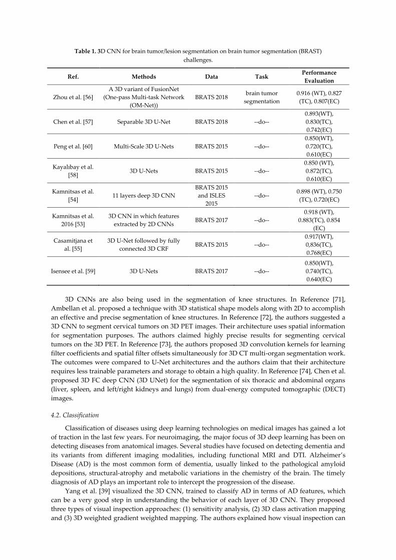
Table 1. 3D CNN for brain tumor/lesion segmentation on brain tumor segmentation (BRAST)

challenges.

Ref. Methods Data Task Performance

Evaluation

Zhou et al. [56]

A 3D variant of FusionNet

(One-pass Multi-task Network

(OM-Net))

BRATS 2018 brain tumor

segmentation

0.916 (WT), 0.827

(TC), 0.807(EC)

Chen et al. [57] Separable 3D U-Net BRATS 2018 --do--

0.893(WT),

0.830(TC),

0.742(EC)

Peng et al. [60] Multi-Scale 3D U-Nets BRATS 2015 --do--

0.850(WT),

0.720(TC),

0.610(EC)

Kayalıbay et al.

[58] 3D U-Nets BRATS 2015 --do--

0.850 (WT),

0.872(TC),

0.610(EC)

Kamnitsas et al.

[54] 11 layers deep 3D CNN

BRATS 2015

and ISLES

2015

--do-- 0.898 (WT), 0.750

(TC), 0.720(EC)

Kamnitsas et al.

2016 [53]

3D CNN in which features

extracted by 2D CNNs BRATS 2017 --do--

0.918 (WT),

0.883(TC), 0.854

(EC)

Casamitjana et

al. [55]

3D U-Net followed by fully

connected 3D CRF BRATS 2015 --do--

0.917(WT),

0,836(TC),

0.768(EC)

Isensee et al. [59] 3D U-Nets BRATS 2017 --do--

0.850(WT),

0.740(TC),

0.640(EC)

3D CNNs are also being used in the segmentation of knee structures. In Reference [71],

Ambellan et al. proposed a technique with 3D statistical shape models along with 2D to accomplish

an effective and precise segmentation of knee structures. In Reference [72], the authors suggested a

3D CNN to segment cervical tumors on 3D PET images. Their architecture uses spatial information

for segmentation purposes. The authors claimed highly precise results for segmenting cervical

tumors on the 3D PET. In Reference [73], the authors proposed 3D convolution kernels for learning

filter coefficients and spatial filter offsets simultaneously for 3D CT multi-organ segmentation work.

The outcomes were compared to U-Net architectures and the authors claim that their architecture

requires less trainable parameters and storage to obtain a high quality. In Reference [74], Chen et al.

proposed 3D FC deep CNN (3D UNet) for the segmentation of six thoracic and abdominal organs

(liver, spleen, and left/right kidneys and lungs) from dual-energy computed tomographic (DECT)

images.

4.2. Classification

Classification of diseases using deep learning technologies on medical images has gained a lot

of traction in the last few years. For neuroimaging, the major focus of 3D deep learning has been on

detecting diseases from anatomical images. Several studies have focused on detecting dementia and

its variants from different imaging modalities, including functional MRI and DTI. Alzheimer’s

Disease (AD) is the most common form of dementia, usually linked to the pathological amyloid

depositions, structural-atrophy and metabolic variations in the chemistry of the brain. The timely

diagnosis of AD plays an important role to intercept the progression of the disease.

Yang et al. [39] visualized the 3D CNN, trained to classify AD in terms of AD features, which

can be a very good step in understanding the behavior of each layer of 3D CNN. They proposed

three types of visual inspection approaches: (1) sensitivity analysis, (2) 3D class activation mapping

and (3) 3D weighted gradient weighted mapping. The authors explained how visual inspection can

improve accuracy and aid in deciding the 3D CNN architecture. In their work, some well-known

baseline 2D deep architectures, such as VGGNet and ResNet, were converted to their 3D

counterparts, and the classification of AD was performed using MRI data from the Alzheimer’s

Disease Neuroimaging Initiative (ADNI). In Reference [75], the authors trained an auto-encoder to

derive an embedding from the input features of 3D patches. These features were extracted from the

preprocessed MRI scans downloaded from the ADNI dataset. Their work demonstrated an

improvement in results in comparison to the 2D approaches available in the literature. In Reference

[76], the authors stacked recurrent neural network (long short-term memory) layers on 3D CNN

layers for AD classification tasks using PET and MRI data. The 3D fully connected CNN layers

obtained deep feature representations and the LSTM was applied on these features to improve the

performance. In Reference [77], a deep 3D CNN was researched on a sizeable dataset for the

classification of AD. Gao et al. [78] showed 87.7% accuracy in the classification of AD, lesion and

normal aging by implementing a seven-layer deep 3D CNN on 285 volumetric CT head scans from

Navy General hospital, China. In this study, the authors also compared their results from 3D CNN

with hand-crafted features of 3D scale-invariant Fourier transform (SIFT) and showed that the

proposed 3D CNN approach gives around four percent higher classification accuracy.

Table 2. 3D CNN for classification tasks in medical imaging.

Ref. Task Model Data Performance Measures

Yang et al.

[39]

AD

classification

3D VggNet, 3D

Resnet

MRI scans from ADNI

dataset (47 AD, 56 NC)

86.3% AUC using 3D

VggNet and 85.4% AUC

using 3D ResNet

Kruthika et

al. [75] --do--

3D capsule

network, 3D CNN

MRI scans from ADNI

dataset (345 AD, NC, 605,

and 991MCI)

Acc. for AD/MCI/NC

89.1%

Feng et al.

[76] --do-- 3D CNN + LSTM

PET + MRI scans from ADNI

dataset (93 AD, 100 NC)

Acc. 65.5% (sMCI/NC),

86.4% (pMCI/NC), and

94.8 % (AD/NC)

Wegmayr et

al. [77] --do-- 3D CNN

ADNI and AIBL data sets,

20000 T1 scans

Acc. 72% (MCI/AD), 86 %

(AD/NC), and 67 %

(MCI/NC)

Oh et al.

[84] --do--

3D CNN +transfer

learning

MRI scans from the ADNI

dataset (AD 198, NC 230,

pMCI 166, and sMCI 101) at

baseline.

74% (pMCI/sMCI), 86%

(AD/NC), 77%

(pMCI/NC)

Parmar et

al. [10] --do-- 3D CNN

fMRI scans from ADNI

dataset

(30 AD, 30 NC)

Classification acc. 94.85 %

(AD/NC)

Nie et al.

[79] Brain tumor

3D CNN with

learning

supervised

features

Private, 69 patient (T1 MRI,

fMRI, and DTI) Classification acc. 89.85 %

Amidi et al.

[85] Protein shape 2-layer 3D CNN

63,558 enzymes from PDB

datasets Classification acc. 78%

Zhou et al.

[80] Breast cancer

Weakly

supervised 3D

CNN

Private, 1537 female patient Classification acc. 78%

83.7%

Besides detecting AD using head MRI (or other modalities), multiple studies have been

performed to detect diseases from varied organs in the body. Nie et al. [79] took advantage of the 3D

aspect of MRI by training a 3D CNN to evaluate the survival in patients going through high-grade

gliomas. Zhou et al. [80] proposed a weakly-supervised 3D CNN for breast cancer detection.

However, there are several limitations of the study: (1) the data was selective in nature, (2) the

proposed architecture was only able to detect the tumor with high probability and (3) only structural

features were used for the experiments. Jnawali et al. [41] demonstrated the performance of 3D CNN

in the classification of CT brain hemorrhage scans. The authors constructed three versions of the 3D

architectures based on CNNs. Two of these architectures are 3D versions of the VggNet and

GoogLeNet. This unique research was done on a large private dataset and about 87.8% accuracy was

demonstrated. In Reference [9], Ker et al. developed a three-layer shallow 3D CNN for brain

hemorrhage classification. The proposed network was giving state-of-the-art results with small

training time when compared to 3D VGGNet and 3D GoogLeNet. Ha et al. [81] modified 2D U-Net

into 3D CNN to quantify the breast MRI fibro-glandular tissue (FGT) and background parenchymal

enhancement (BPE). In Reference [58], Nie et al. proposed a multi-channel structure of 3D CNN for

survival time prediction of Glioblastoma patients using multi-modal head images (T1 weighted MRI

and diffusion tensor imaging, DTI). Recently, in Reference [82], the author presented a hybrid model

for the classification and prediction of lymph node metastasis (LNM) in head and neck cancer. They

combined the outputs of MaO-radiomics and 3D CNN architecture by using an evidential reasoning

(ER) fusion strategy. In Reference [83], the authors presented a 3D CNN for predicting the maximum

standardized uptake value of lymph nodes in patients suffering from cancer using CT images from a

PET/CT examination. We summarized some important developments in 3D deep learning models

for classification tasks in medical imaging in Table 2.

4.3. Detection and Localization

Cerebral Microbleeds (CMBs) are small foci of chronic hemorrhages that can occur in the

normal brains due to structural abnormalities of small blood vessels in the brain. Due to the

differential properties of blood, MRI can detect CMBs. However, detecting cerebral

micro-hemorrhages in brain tissue is a difficult and time-consuming task for radiologists, while

recent studies employed 3D deep architectures to detect CMBs. Dou et al. [86] proposed a two-stage

fully connected 3D CNN architecture to detect CMBs from the dataset of MRI

susceptibility-weighted images (SWI). The network reduced many false-positive candidates. For

training purposes, multiple 3D cubes were extracted from the preprocessed dataset. This study also

examined the effect of the size of 3D patches on network performance. The study also focuses on the

higher performance of 3D architectures in the detection of CMBs in comparison to their 2D

architectures, such as Random Forest and 2D-CNN-SVM. Dou et al. further employed a fully 3D

CNN to detect microscopic areas of a brain hemorrhage on MRI brain scans. This method had a

sensitivity of 93% and outperformed prior methods of detection. Standvoss et al. [87] detected CMBs

in traumatic brain injury. In their study, the authors prepared three types of 3D architectures with

varying depths, i.e., three, five and eight layers. These models were quite simple and straight

forward, with an overall best accuracy of 87%. The drawback of these studies was that they utilized a

small dataset for training the network. In Reference [88], the author presented a 3D CNN to forecast

the route and radius of an artery at any given point in a cardiac CT angiography image, which

depends on the local image patch. This approach can precisely and effectively predict the path and

the radius of coronary arteries through the details extracted from the image files.

Lung cancer is also the foremost cause of death worldwide. Nonetheless, the survival rate

would be increased if we could detect lung cancer at an early stage. Subsequently, the past decade

has seen considerable research into the detection, classification and localization of lung nodules

using 3D deep learning approaches. In Reference [89], Anirudh et al. first proposed a 3D CNN for

lung nodule detection using weakly labeled data. In 3D medical imaging, data labeling is quite

complex and time-consuming when compared to 2D image modalities. The authors used a

single-pixel point to unveil the data and used this single point information to grow the region using

the thresholding and filtering of super-pixels. This process was performed on 2D slices and these

slices were combined using 3D Gaussian filtering. Using the proposed 3D CNN, the authors showed

an 0.80 sensitivity with 10 false positives per scan. However, the architecture of 3D CNN was not

very deep in this work. Furthermore, the data were very small (70 scans), and therefore, the results

may be biased. Dou et al. [90] exploited 3D CNN with multilevel contextual information for the

false-positive reduction in pulmonary nodules in volumetric CT scans. The authors used 887 CT

scans from a publicly available LIDC-IDRI dataset (LUNA16 challenge). Huang et al. [91] exploited

3D CNN to detect lung nodules in low-dose CT chest scans. The positive and negative cubes were

extracted from CT data using a priori knowledge about the data and confounding the anatomical

structure. The proposed design effectively reduced the complexity and showed a significant

improvement in performance. Compared to the baseline approach, their approach showed 90%

sensitivity, while a reduction in false positives from 35 to 5. Gruetzemacher et al. [12] used 3D UNet

with residual blocks for detecting pulmonary nodules in CT scans from the LIDC-IDRI dataset. The

authors used two 3D CNN models, one for each essential task, i.e., candidate generation and

false-positive reduction. The model was experimented and evaluated with 888 CT scans. On the test

data, an overall 89.3% detection and 1.79 false-positive rate was obtained. To tackle large variations

in the size of the nodules, Gu et al. [92] proposed multi-scale prediction with a fusion scheme for 3D

CNN (Figure 7). This work was also a part of the LUNA16 challenge and achieved 92.9% sensitivity

with four false positives per scan.

Figure 7. The basic procedure for lung nodule detection. The figure is modified from Reference [92].

To deal with the issue of limited data, Winkels and Cohen [93] proposed a 3D group

convolutional neural network (3D-GCNNs). In this work, 3D rotations and reflections were used as

input instead of translating a filter on the input (as in traditional 3D CNN). The authors showed that

this approach needs only one-tenth of the data used in the conventional approach to obtain the same

performance. In another work, Gong et al. [94] suggested a 3D CNN by exploiting the properties of

ResNet and squeeze and excitation (SE) strategy. A 3D region proposal network using a UNet like

structure was used for nodule detection, and then a 3D CNN was used for the reduction of false

positives. The SE block increases the representation power of the network by focusing on

channel-wise information. On the LIDC-IDRI dataset, 95.7% sensitivity was achieved with four false

positives per scan. Pezeshk et al. [24] presented two-stage 3D CNN for automatic pulmonary nodule

detection in CT scans. The first stage of 3D CNN was used for screening and candidate generation.

The second stage was an ensemble of 3D CNNs trained with both positive and negative augmented

patches.

The localization of biological architectures is a basic requirement for various initiatives in

medical image investigation. Localization might be a hassle-free process for the radiologist, but it is

usually a hard task for NNs that are vulnerable to variation in medical images induced by

dissimilarities in the image acquisition process, structures and pathological differences among

patients. Generally, a 3D volume is required for localization in medical images. Several techniques

treat the 3D space as an arrangement of 2D orthogonal planes. Wolterink et al. [95] detected

coronary artery calcium scoring in coronary CT angiography using a CNN based architecture. De

Vos et al. [96] introduced the localization technique using a solitary CNN, and 2D CT image slices

(chest CT, cardiac CT and abdomen CT) as inputs. While this work was related to a 3D localization

approach, they did not use 3D CNN in a real sense. Further, the approach depended heavily on the

accurate recognition of biological structures. Huo et al. [97] utilized the properties of a 3D fully

connected CNN and presented a spatially localized atlas network tiles (SLANT) model for

whole-brain segmentation on high-resolution multi-site images.

Intervertebral discs (IVDs) are modest joint parts that are located in between surrounding

vertebrae and the localization of IVDs, which are usually important for spine disease analysis and

Data augmentation3D Convolutions 3D Pooling Flatten

Nodules

Other tissues

Detection

Lung segmentation and 3D

patch extraction

measurement. In Reference [98], the authors presented a 3D detection for multiple brain structures

in fetal neuro-sonography using fully connected CNNs and named it VP-Nets. They explained that

the proposed strategy requires a comparatively less amount of data for training and can learn from

coarsely annotated 3D data. Recently, a 3D CNN, based on regression, has been introduced in

Reference [42] to assess the degree of enlarged perivascular spaces (EPVS) through 2000 basal

ganglia scans from 3D head MRI. In Reference [99], the authors reported the human-level efficiency

of 3D CNN in the landmark detection of clinical 3D CT data. In [100], Saleh et al. proposed a 3D

CNN based regression models for 3D pose estimation of anatomy using T2 weighted imaging. They

showed that the proposed network offers fine initialization for optimization-based techniques to

increase the capture range of slice-to-volume registration. Xiaomeng et al. [101] presented fully

connected, accurate and automatic 3D deep architecture for the localization and segmentation of

IVDs using multimodal MR images. The work shows state-of-the-art performance in the

MICCAI-2016 challenge for IVDs localization and segmentation section with a dice score of 0.912 for

IVD segmentation. Cardiac magnetic resonance (CMR) imaging is popular in diagnosing various

cardiovascular diseases. Vesel et al. [102] proposed a 3D DR-UNet (modified 3D UNet) for

localization of cardiac structure in MRI volume. The model was evaluated on two datasets: the

Automatic Cardiac Segmentation Challenge (ACDC) STACOM 2017, and Left Atrium Segmentation

Challenge (LASC) STACOM 2018. Their model shows state-of-the-art results in terms of several

performance indices.

4.4. Registration

Medical images of a single subject can be increasingly multi-modal in the same patient from CT,

MRI T1 and MRI T2. Each imaging modality focuses on different features of the subject. Typically, a

clinician is expected to view images of multiple modalities in different orientations to deduce a

match between these images by visual comparison. The clinician is also expected to manually

identify points in these images that have significant signal differences. Thus, two image analysis

problems can be automated. First, the alignment or registration of datasets can be automated, and

second, the automatic alignment of datasets can be made to modalities in which abnormalities are

present. This allows us to identify prominent parts of an image for further review. In recent years,

many efforts have been made in medical image registration using 3D deep learning. For example,

Sokooti et al. successfully used 3D CNN for 3D nonrigid image registration in Reference [103]. For

training the 3D CNN, 3D patches were extracted from 3D CT chest images. The network was trained

on artificially generated displacement vector fields. The authors confirmed that their model

outperformed a traditional B-spline registration method and performed on par with

multi-resolution B-spline methods. However, for all the landmarks, multi-resolution B-spline

methods outperformed their approach. Further, the capture range of their approach was limited to

the size of the patches. A possible solution to increase the capture range of their method is to

increase the size of the patches or to add more scales to the network. Torng et al. [104] showed the

effectiveness of a shallow 3D CNN with three convolutional layers with filter sizes of 3x3, followed

by 3D max-pooling layers and two fully connected layers with dropout for analyzing the interaction

of amino acids to their neighboring microenvironment. The authors also proposed the CNN

activation visualization technique called the atom importance map. For training and test data, 3D

patches (local box) were extracted from the protein structure. Furthermore, the local structure was

decomposed into five channels (inputs to 3D CNN), including oxygen, carbon, nitrogen and

sulphur. The model shows a performance improvement of 20% when compared to the structure

based on handcrafted biochemical features. To deal with the memory issue and computational cost,

Blendowski and Heinrich [105] suggested a combination of MRF-based deformable registration and

3D CNN descriptors for lung motion estimation on non-rigidly deformed chest CT images.

There are several freely available medical image registration software and toolkits such as

SimpleITK [106] and ANTs [107]. Typically, the registration process to these toolkits is done by

iteratively updating the transformational parameters until a predefined similarity metric is

optimized. These methods show a decent performance. However, their performance is limited by

their slow registration process. To overcome this issue, several attempts have been made in the

literature based on deep learning and 3D deep learning. Recently, Chee and Wu [108] used CNN as

an affine image registration network (AIRNet) for MR brain image registration. AirNet, proposed by

the authors, works in two parts, i.e., encoder and regressor. The architecture of the encoder part was

drawn from DenseNet [109] with some modifications in filter structures (a mixture of 2D and 3D

filters). The output of the encoder was then given to the regressor part. The proposed framework

was compared to conventional registration algorithms used in the well-known software package

SimpleITK [106]. The proposed framework shows significant improvements in Jac and dH. The

authors claim that this method was 100 times faster than other traditional methods. Zhou et al. [110]

proposed 3D CNN for serial electron microscopy images (experiments were performed on two

databases, Cremi and FIB25) registration. Recently, Zhao et al. [111] presented a 3D Volume

Tweening Network (VTN) for 3D medical image (liver CT and brain MRI dataset) registration in an

unsupervised manner. Compared to the traditional optimization approaches (ANTs [107], Elastix

[112] and VoxelMorph-2 [113]), their method was 880 times faster, with state-of-the-art performance.

In Reference[114], Wang et al. proposed a dynamic 2D/3D registration algorithm for accurate

alignment between 2-D and 3-D images for fusion applications. The model introduced by the author

was based on point-to-plane correspondence (PPC) and its dynamic registration procedure was fully

capable of recovering 3-D motion from single-2D view images.

5. Challenges and Conclusions

It takes a large number of training samples to train deep learning models [53,115,116]. This is

further strengthened by the recent successes of deep learning models trained on large datasets like

the ImageNet. However, it is still ambiguous whether deep learning models can successfully work

with smaller datasets, as in the case of medical images. The ambiguity is caused by the nature and

characteristics of medical images. For example, the images from the ImageNet dataset possess large

variations in their appearance (e.g., light, intensity, edges, color, etc.) [14,36,117–119] since the

images were taken at different angles and distances, and have several different features that are

completely different from medical images. Therefore, networks that need to learn meaningful

representations of these images require large training parameters and thus training samples.

However, in the case of medical images, there is much less variation in comparison to traditional

image datasets [120]. In this regard, the process of fine-tuning of 3D CNN models, which are already

trained on natural image datasets, can be applied to medical images [14,36,117–119,121,122]. This

process, known as transfer learning, has been successfully applied to many areas of medical

imaging.

Regardless of their high computational complexity, 3D deep networks have shown incredible

performance in diverse domains. 3D deep networks require a large number of training parameters,

especially in the case of 3D medical images, where the depth of the image volume varies from 20 to

400 slices per scan [36,79,123,124], with each scan containing very fine and important information

about the patient. Usually, high-resolution scan volumes are of the size 512 × 512, and need to be

downsampled before being fed into the 3D network to reduce the computational cost. Researchers

generally use interpolation techniques to reduce the overall size of these medical image volumes, but

come at the cost of significant information loss. There are also restrictions on the resizing of the

medical image volume without the loss of significant information. This is still an unexplored area

and there is further research scope.

While the number of trainable parameters of convolutional layers is independent of the input

size, the number of trainable parameters in the subsequent fully connected layers depend on the

output of the convolution layers. This often leads to intractable models due to a large number of

trainable weights when the input images are fed into 3D CNN models without any down-sampling.

However, this is not an issue in the case of 2D images, which have smaller latent representations that

are learnt by convolution filters. This makes it harder (and more GPU intensive) to train 3D deep

networks based on CNNs. The inception module by GoogLeNet can be further explored to address

computational complexity in 3D medical image analysis. In recent times, many computational 3D

imaging techniques have appeared in the literature where the acquired data is not necessarily a

traditional image. Sometimes raw data may be suitable for a few applications in deep learning. For

example, single-pixel imaging techniques are popular in unconventional applications, including

X-rays. A brief review of various applications of single-pixel imaging in 3D reconstruction can be

found in Reference [125]. Ghost imaging is also popular for image reconstruction, such as lens-less

imaging and X-ray imaging. In order to enhance the quality of image reconstruction, Wang et al.

[126] applied deep learning on the images reconstructed from traditional ghost imaging.

Indeed, in the deep learning context, learning the correct features might sound unconventional

because we cannot be sure if the models learn features that are discriminating for the condition or

just overfit on some specific features for the given dataset. CNNs can handle raw image data and

they do not need to be handcrafted [11,117]. It is the responsibility of CNN to discover the right

features from the data. While CNNs have made encoding the raw features in a latent space very

convenient, it is important to understand whether the features learned by CNN are generalizable

across datasets. Machine learning models often overfit on training samples as they only perform

well on the test samples from the training dataset. This issue is acute in the case of medical imaging

applications where there are issues with scanner variability, scan acquisition settings, subject

demography, and heterogeneity in disease characteristics across subjects. Therefore, it is important

to decode the trained network using model interpretability approaches and validate the important

features learned by the network [127]. It also becomes important to report testing results with an

external dataset whose samples were not used for training. However, this may not always be

possible because of the paucity of datasets for training and testing.

Finally, the ultimate challenge is to go beyond a human-level performance. Researchers are

working on reaching human-level performance for many tasks (known as Artificial General

Intelligence) [35,53,128,129]. However, the lack of labeled images, high costs involved in labeling the

datasets and lack of consensus among experts in validating the assigned labels [38,130,131] are some

present challenges in the field. These issues force us to consider using reliable data augmentation

methods and to generate samples with known ground-truths. In this regard, generative adversarial

networks (GAN) [132], especially CycleGANs for cross-modal image synthesis, offer a viable

approach for synthesizing data. They are being used to produce pseudo images that are highly

similar to the original dataset.

Author Contributions: All authors conceptualized the ideas and conducted the literature search, prepared the

figures, tables, and drafted the manuscript. All authors have read and approved the manuscript.

Funding: Authors acknowledge the support from Lee Kong Chian School of Medicine and Data Science and AI

Research (DSAIR) center of Nanyang Technological University Singapore (Project Number

ADH-11/2017-DSAIR).

PP and BG also acknowledges the support from the Cognitive Neuro Imaging Centre (CONIC) at Nanyang

Technological University Singapore.

Conflicts of Interest: The authors declare no conflict of interest.

References

1. Doi, K. Computer-Aided Diagnosis in Medical Imaging: Historical Review, Current Status and Future

Potential. Comput. Med. Imaging Graph. 2007, 31, 198–211, doi:10.1016/j.compmedimag.2007.02.002.

2. Miller, A.S.; Blott, B.H.; hames, T.K. Review of neural network applications in medical imaging and

signal processing. Med. Biol. Eng. Comput. 1992, 30, 449–464, doi:10.1007/BF02457822.

3. Siedband, M.P. Medical imaging systems. Medical Instrumentation; 3rd ed.; 1998;

4. Prince, J.; Links, J. Medical imaging signals and systems. Med. Imaging 2006, 315–379, doi:0132145189.

5. Shapiro, R.S.; Wagreich, J.; Parsons, R.B.; Stancato-Pasik, A.; Yeh, H.C.; Lao, R. Tissue harmonic

imaging sonography: Evaluation of image quality compared with conventional sonography. Am. J.

Roentgenol. 1998, 171, 1203–1206, doi:10.2214/ajr.171.5.9798848.

6. Matsumoto, K.; Jinzaki, M.; Tanami, Y.; Ueno, A.; Yamada, M.; Kuribayashi, S. Virtual Monochromatic

Spectral Imaging with Fast Kilovoltage Switching: Improved Image Quality as Compared with That

Obtained with Conventional 120-kVp CT. Radiology 2011, 259, 257–262, doi:10.1148/radiol.11100978.

7. Thibault, J.B.; Sauer, K.D.; Bouman, C.A.; Hsieh, J. A three-dimensional statistical approach to

improved image quality for multislice helical CT. Med. Phys. 2007, 34, 4526–4544, doi:10.1118/1.2789499.

8. Marin, D.; Nelson, R.C.; Schindera, S.T.; Richard, S.; Youngblood, R.S.; Yoshizumi, T.T.; Samei, E.

Low-Tube-Voltage, High-Tube-Current Multidetector Abdominal CT: Improved Image Quality and

Decreased Radiation Dose with Adaptive Statistical Iterative Reconstruction Algorithm—Initial Clinical

Experience. Radiology 2010, 254, 145–153, doi:10.1148/radiol.09090094.

9. Ker, J.; Singh, S.P.; Bai, Y.; Rao, J.; Lim, T.; Wang, L. Image Thresholding Improves 3-Dimensional

Convolutional Neural Network Diagnosis of Different Acute Brain Hemorrhages on Computed

Tomography Scans. Sensors 2019, 19, 2167, doi:10.3390/s19092167.

10. Parmar, H.S.; Nutter, B.; Long, R.; Antani, S.; Mitra, S. Deep learning of volumetric 3D CNN for fMRI in

Alzheimer’s disease classification. In Proceedings of the Medical Imaging 2020: Biomedical

Applications in Molecular, Structural, and Functional Imaging; Gimi, B.S., Krol, A., Eds.; SPIE; Vol.

11317, p. 11.

11. Shen, D.; Wu, G.; Suk, H.-I. Deep Learning in Medical Image Analysis. Annu. Rev. Biomed. Eng. 2017, 19,

221–248, doi:10.1146/annurev-bioeng-071516-044442.

12. Gruetzemacher, R.; Gupta, A.; Paradice, D. 3D deep learning for detecting pulmonary nodules in CT

scans. J. Am. Med. Informatics Assoc. 2018, 25, 1301–1310, doi:10.1093/jamia/ocy098.

13. Wang, S.H.; Phillips, P.; Sui, Y.; Liu, B.; Yang, M.; Cheng, H. Classification of Alzheimer’s Disease Based

on Eight-Layer Convolutional Neural Network with Leaky Rectified Linear Unit and Max Pooling. J.

Med. Syst. 2018, 42, 85, doi:10.1007/s10916-018-0932-7.

14. Krizhevsky, A.; Sulskever, Ii.; Hinton, G.E. ImageNet Classification with Deep Convolutional Neural

Networks. Adv. Neural Inf. Process. Syst. 2012, 60, 84–90, doi:10.1145/3065386.

15. Szegedy, C.; Liu, W.; Jia, Y.; Sermanet, P.; Reed, S.; Anguelov, D.; Erhan, D.; Vanhoucke, V.; Rabinovich,

A. Going deeper with convolutions. In Proceedings of the Proceedings of the IEEE Computer Society

Conference on Computer Vision and Pattern Recognition; IEEE Computer Society, 2015; Vol.

07-12-June, pp. 1–9.

16. Hoi, S.C.H.; Jin, R.; Zhu, J.; Lyu, M.R. Batch mode active learning and its application to medical image

classification. In Proceedings of the ACM International Conference Proceeding Series; New York, 2006;

Vol. 148, pp. 417–424.

17. Rahman, M.M.; Bhattacharya, P.; Desai, B.C. A Framework for Medical Image Retrieval Using Machine

Learning and Statistical Similarity Matching Techniques With Relevance Feedback. IEEE Trans. Inf.

Technol. Biomed. 2007, 11, 58–69, doi:10.1109/TITB.2006.884364.

18. Wernick, M.; Yang, Y.; Brankov, J.; Yourganov, G.; Strother, S. Machine Learning in Medical Imaging.

IEEE Signal Process. Mag. 2010, 27, 25–38, doi:10.1109/MSP.2010.936730.

19. Criminisi, A., Shotton, J., & Konukoglu, E. Decision forests: A unified framework for classification,

regression, density estimation, manifold learning and semi-supervised learning. Found. Trends®

Comput. Graph. Vision, 2012, 7, 81–227.

20. Singh, S.P.; Urooj, S. An Improved CAD System for Breast Cancer Diagnosis Based on Generalized

Pseudo-Zernike Moment and Ada-DEWNN Classifier. J. Med. Syst. 2016, 40, 105,

doi:10.1007/s10916-016-0454-0.

21. Urooj, S.; Global, S.S.-C. for S.; 2015, undefined Rotation invariant detection of benign and malignant

masses using PHT. ieeexplore.ieee.org.

22. Ji, S.; Xu, W.; Yang, M.; Yu, K. 3D Convolutional Neural Networks for Human Action Recognition. IEEE

Trans. Pattern Anal. Mach. Intell. 2013, 35, 221–231, doi:10.1109/TPAMI.2012.59.

23. Moher, D.; Liberati, A.; Tetzlaff, J.; Altman, D.G.; Altman, D.; Antes, G.; Atkins, D.; Barbour, V.;

Barrowman, N.; Berlin, J.A.; et al. Preferred reporting items for systematic reviews and meta-analyses:

The PRISMA statement. PLoS Med. 2009, 6, e1000097.

24. Pezeshk, A.; Hamidian, S.; Petrick, N.; Sahiner, B. 3-D Convolutional Neural Networks for Automatic

Detection of Pulmonary Nodules in Chest CT. IEEE J. Biomed. Heal. Informatics 2019, 23, 2080–2090,

doi:10.1109/JBHI.2018.2879449.

25. Springenberg, J.T.; Dosovitskiy, A.; Brox, T.; Riedmiller, M. Striving for simplicity: The all convolutional

net. In Proceedings of the 3rd International Conference on Learning Representations, ICLR 2015 -

Workshop Track Proceedings; 2015.

26. Kukačka, J.; Golkov, V.; Cremers, D. Regularization for Deep Learning: A Taxonomy. arXiv Prepr.

arXiv1710.10686 2017.

27. Srivastava, N.; Hinton, G.; Krizhevsky, A.; Salakhutdinov, R. Dropout: A Simple Way to Prevent Neural

Networks from Overfitting; 2014; Vol. 15;.

28. Ioffe, S.; Szegedy, C. Batch normalization: Accelerating deep network training by reducing internal

covariate shift. In Proceedings of the 32nd International Conference on Machine Learning, ICML 2015;

International Machine Learning Society (IMLS), 2015; Vol. 1, pp. 448–456.

29. Simonyan, K.; Zisserman, A. Very deep convolutional networks for large-scale image recognition. In

Proceedings of the 3rd International Conference on Learning Representations, ICLR 2015 - Conference

Track Proceedings; 2015.

30. Szegedy, C.; Vanhoucke, V.; Ioffe, S.; Shlens, J.; Wojna, Z. Rethinking the Inception Architecture for

Computer Vision. In Proceedings of the Proceedings of the IEEE Computer Society Conference on

Computer Vision and Pattern Recognition; 2016; Vol. 2016-Decem, pp. 2818–2826.

31. Szegedy, C.; Ioffe, S.; Vanhoucke, V.; Alemi, A.A. Inception-v4, inception-ResNet and the impact of

residual connections on learning. In Proceedings of the 31st AAAI Conference on Artificial Intelligence,

AAAI 2017; 2017; pp. 4278–4284.

32. He, K.; Zhang, X.; Ren, S.; Sun, J. Deep residual learning for image recognition. In Proceedings of the

Proceedings of the IEEE Computer Society Conference on Computer Vision and Pattern Recognition;

IEEE Computer Society, 2016; Vol. 2016-Decem, pp. 770–778.

33. Ronneberger, O.; Fischer, P.; Brox, T. U-net: Convolutional networks for biomedical image

segmentation. In Proceedings of the Lecture Notes in Computer Science (including subseries Lecture

Notes in Artificial Intelligence and Lecture Notes in Bioinformatics); Springer, Cham.: Munich,

Germany, 2015; Vol. 9351, pp. 234–241.

34. Çiçek, Ö.; Abdulkadir, A.; Lienkamp, S.S.; Brox, T.; Ronneberger, O. 3D U-Net: Learning Dense

Volumetric Segmentation from Sparse Annotation. In Proceedings of the Medical Image Computing

and Computer-Assisted Intervention; Springer, Cham.: Athens, Greece, 2016; Vol. 9901 LNCS, pp. 424–

432.

35. Ker, J.; Wang, L.; Rao, J.; Lim, T. Deep Learning Applications in Medical Image Analysis. IEEE Access

2018, 1–1, doi:10.1109/ACCESS.2017.2788044.

36. Burt, J. Volumetric quantification of cardiovascular structures from medical imaging. Google Patents

2018.

37. Esteban, O.; Markiewicz, C.J.; Blair, R.W.; Moodie, C.A.; Isik, A.I.; Erramuzpe, A.; Kent, J.D.; Goncalves,

M.; DuPre, E.; Snyder, M. and; et al. fmriprep: A Robust Preprocessing Pipeline for fMRI Data —

fmriprep version documentation. Nat. Methods 2019, 111–116.

38. Alansary, A.; Kamnitsas, K.; Davidson, A.; Khlebnikov, R.; Rajchl, M.; Malamateniou, C.; Rutherford,

M.; Hajnal, J. V.; Glocker, B.; Rueckert, D.; et al. Fast Fully Automatic Segmentation of the Human

Placenta from Motion Corrupted MRI. In Proceedings of the International Conference on Medical

Image Computing and Computer-Assisted Intervention; Springer, Cham, 2016; pp. 589–597.

39. Yang, C.; Rangarajan, A.; Ranka, S. Visual Explanations From Deep 3D Convolutional Neural Networks

for Alzheimer’s Disease Classification. AMIA ... Annu. Symp. proceedings. AMIA Symp. 2018, 2018, 1571–

1580.

40. Jones, D.K.; Griffin, L.D.; Alexander, D.C.; Catani, M.; Horsfield, M.A.; Howard, R.; Williams, S.C.R.

Spatial Normalization and Averaging of Diffusion Tensor MRI Data Sets. Neuroimage 2002, 17, 592–617,

doi:10.1006/nimg.2002.1148.

41. Jnawali, K.; Arbabshirani, M.; Rao, N. Deep 3D convolution neural network for CT brain hemorrhage

classification. In Proceedings of the Medical Imaging 2018: Computer-Aided Diagnosis; SPIE; p.

105751C.

42. Dubost, F.; Adams, H.; Bortsova, G.; Ikram, M. 3D Regression Neural Network for the Quantification of

Enlarged Perivascular Spaces in Brain MRI. Med. Image Anal. 2019, 51, 89–100.

43. Lian, C.; Liu, M.; Zhang, J.; Zong, X.; Lin, W.; Shen, D. Automatic Segmentation of 3D Perivascular

Spaces in 7T MR Images Using Multi-Channel Fully Convolutional Network. Elsevier 2018, 5–7.

44. Pauli, R.; Bowring, A.; Reynolds, R.; Chen, G.; Nichols, T.E.; Maumet, C. Exploring fMRI results space:

31 variants of an fMRI analysis in AFNI, FSL, and SPM. Front. Neuroinform. 2016, 10, 24,

doi:10.3389/fninf.2016.00024.

45. Parker, D.; Liu, X.; Razlighi, Q.R. Optimal slice timing correction and its interaction with fMRI

parameters and artifacts. Med. Image Anal. 2017, 35, 434–445, doi:10.1016/j.media.2016.08.006.

46. Goebel, R. BrainVoyager - Past, present, future. Neuroimage 2012, 62, 748–756,

doi:10.1016/j.neuroimage.2012.01.083.

47. Maes, F.; Collignon, A.; Vandemeulen, D.; Marchal, G.; Suetens, P. Multimodality image registration by

maximization of mutual information. ieeemi 1997, 16, 187–198.

48. J.B.A., M.; A., V.M. A survey of medical image registration. Med Image Anal 1998, 2, 1–36,

doi:http://dx.doi.org/10.1016/S1361-8415(01)80026-8.

49. Pluim, J.P.W.; Maintz, J.B.A.; Viergever, M.A. Interpolation Artefacts in Mutual Information Based

Image Registration. Comput. Vis. Image Underst. 2000, 77, 211–232.

50. Penney, G.P.; Weese, J.; Little, J.A.; Desmedt, P.; Hill, D.L.G.; Hawkes, D.J. A comparison of similarity

measures for use in 2-D-3-D medical image registration. Med. Imaging, IEEE Trans. 1998, 17, 586–595,

doi:10.1109/42.730403.

51. Ahmed, Mohamed N., Sameh M. Yamany, Nevin Mohamed, Aly A. Farag, and T.M. A modified

fuzzy c-means algorithm for bias field estimation and segmentation of MRI data. IEEE Trans. Med.

Imaging 2002, 21, 193–199.

52. Li, C.; Xu, C.; Anderson, A.W.; Gore, J.C. MRI tissue classification and bias field estimation based on

coherent local intensity clustering: A unified energy minimization framework. In Proceedings of the

Lecture Notes in Computer Science (including subseries Lecture Notes in Artificial Intelligence and

Lecture Notes in Bioinformatics); Springer, Berlin, Heidelberg.: Williamsburg, VA, USA, 2009; Vol. 5636

LNCS, pp. 288–299.

53. Kamnitsas, K.; Ferrante, E.; Parisot, S.; Ledig, C.; Nori, A. V.; Criminisi, A.; Rueckert, D.; Glocker, B.

DeepMedic for Brain Tumor Segmentation. In Proceedings of the International Workshop on

Brainlesion: Glioma, Multiple Sclerosis, Stroke and Traumatic Brain Injuries; Springer, Cham., 2016; pp.

138–149.

54. Kamnitsas, K.; Ledig, C.; Newcombe, V.F.J.; Simpson, J.P.; Kane, A.D.; Menon, D.K.; Rueckert, D.;

Glocker, B. Efficient multi-scale 3D CNN with fully connected CRF for accurate brain lesion

segmentation. Med. Image Anal. 2017, 36, 61–78, doi:10.1016/j.media.2016.10.004.

55. Casamitjana, A.; Puch, S.; Aduriz, A.; Vilaplana, V. 3D convolutional neural networks for brain tumor

segmentation: A comparison of multi-resolution architectures. In Proceedings of the Lecture Notes in

Computer Science (including subseries Lecture Notes in Artificial Intelligence and Lecture Notes in

Bioinformatics); Springer, Cham.: Athens, Greece, 2016; Vol. 10154 LNCS, pp. 150–161.

56. Zhou, C.; Ding, C.; Wang, X.; Lu, Z.; Tao, D. One-pass Multi-task Networks with Cross-task Guided

Attention for Brain Tumor Segmentation. IEEE Trans. Image Process. 2020, 1–1,

doi:10.1109/TIP.2020.2973510.

57. Chen, W.; Liu, B.; Peng, S.; Sun, J.; Qiao, X. S3D-UNET: Separable 3D U-Net for brain tumor

segmentation. In Proceedings of the International MICCAI Brainlesion Workshop; Springer, Cham.:

Granada, Spain, 2019; Vol. 11384 LNCS, pp. 358–368.

58. Kayalibay, B.; Jensen, G.; van der Smagt, P. CNN-based Segmentation of Medical Imaging Data. arXiv

Prepr. arXiv1701.03056 2017.

59. Isensee, F.; Kickingereder, P.; Wick, W.; Bendszus, M.; Maier-Hein, K.H. Brain tumor segmentation and

radiomics survival prediction: Contribution to the BRATS 2017 challenge. In Proceedings of the

International MICCAI Brainlesion Workshop; Springer, Cham., 2018; Vol. 10670 LNCS, pp. 287–297.

60. Peng, S.; Chen, W.; Sun, J.; Liu, B. Multi-Scale 3D U-Nets: An approach to automatic segmentation of

brain tumor. Int. J. Imaging Syst. Technol. 2019, 30, 5–17, doi:10.1002/ima.22368.

61. Milletari, F.; Ahmadi, S.A.; Kroll, C., P.; A., R.; V., M.; J., Levin, J.; Dietrich, O.; Ertl-Wagner, B.; Bötzel,

K. and; Navab, N. Hough-CNN: Deep Learning for Segmentation of Deep Brain Regions in MRI and

Ultrasound. Comput. Vis. Image Underst. 2017, 164, 92–102.

62. Dolz, J.; Desrosiers, C. 3D fully convolutional networks for subcortical segmentation in MRI: A

large-scale study. Neuroimage 2017.

63. Sato, D.; Hanaoka, S.; Nomura, Y.; Takenaga, T.; Miki, S.; Yoshikawa, T.; Hayashi, N.; Abe, O. A

primitive study on unsupervised anomaly detection with an autoencoder in emergency head CT

volumes. In Proceedings of the Medical Imaging 2018: Computer-Aided Diagnosis; 2018; p. 60.

64. Dou, Q.; Yu, L.; Chen, H.; Jin, Y.; Yang, X.; … J.Q. 3D deeply supervised network for automated

segmentation of volumetric medical images. Med. Image Anal. 2017, 41, 40–54.

65. Zeng, G.; Yang, X.; Li, J.; Yu, L.; Heng, P.A.; Zheng, G. 3D U-net with multi-level deep supervision:

Fully automatic segmentation of proximal femur in 3D MR images. In Proceedings of the Lecture Notes

in Computer Science (including subseries Lecture Notes in Artificial Intelligence and Lecture Notes in

Bioinformatics); Springer, Cham.: Quebec City, Canada, 2017; Vol. 10541 LNCS, pp. 274–282.

66. Zhu, Z.; Xia, Y.; Shen, W.; Fishman, E.; Yuille, A. A 3D coarse-to-fine framework for volumetric medical

image segmentation. In Proceedings of the Proceedings - 2018 International Conference on 3D Vision,

3DV 2018; 2018; pp. 682–690.

67. Yang, X.; Bian, C.; Yu, L.; Ni, D.; Heng, P.A. Hybrid loss guided convolutional networks for whole heart

parsing. In Proceedings of the International workshop on statistical atlases and computational models

of the heart; Springer, Cham.: Quebec City, Canada, 2017; Vol. 10663 LNCS, pp. 215–223.

68. Roth, H.R.; Oda, H.; Zhou, X.; Shimizu, N.; Yang, Y. Computerized Medical Imaging and Graphics An

application of cascaded 3D fully convolutional networks for medical image segmentation. Comput. Med.

Imaging Graph. 2018, 66, 90–99, doi:10.1016/j.compmedimag.2018.03.001.

69. Yu, L.; Yang, X.; Qin, J.; Heng, P.A. 3D FractalNet: Dense volumetric segmentation for cardiovascular

MRI volumes. In Proceedings of the Lecture Notes in Computer Science (including subseries Lecture

Notes in Artificial Intelligence and Lecture Notes in Bioinformatics); Springer, Cham.: Athens, Greece,

2017; Vol. 10129 LNCS, pp. 103–110.

70. Li, X.; Chen, H.; Qi, X.; Dou, Q.; Fu, C.-W.; Heng, P.A. H-DenseUNet: Hybrid Densely Connected UNet

for Liver and Liver Tumor Segmentation from CT Volumes. IEEE Trans. Med. Imaging 2018,

doi:10.1109/TMI.2018.2845918.

71. Ambellan, F.; Tack, A.; Ehlke, M.; Zachow, S. Automated segmentation of knee bone and cartilage

combining statistical shape knowledge and convolutional neural networks: Data from the

Osteoarthritis Initiative. Med. Image Anal. 2019, 52, 109–118, doi:10.1016/j.media.2018.11.009.

72. Chen, Liyuan, Chenyang Shen, Zhiguo Zhou, Genevieve Maquilan, Kevin Albuquerque, Michael R.

Folkert, and J.W. Automatic PET cervical tumor segmentation by deep learning with prior

information. In Proceedings of the Physics in medicine and biology; 2019; p. 111.

73. Heinrich, M.P.; Oktay, O.; Bouteldja, N. OBELISK-Net: Fewer layers to solve 3D multi-organ

segmentation with sparse deformable convolutions. Med. Image Anal. 2019, 54, 1–9,

doi:10.1016/j.media.2019.02.006.

74. Chen, S.; Zhong, X.; Hu, S.; Dorn, S.; Kachelrieß, M.; Lell, M.; Maier, A. Automatic multi-organ

segmentation in dual-energy CT (DECT) with dedicated 3D fully convolutional DECT networks. Med.

Phys. 2020, 47, 552–562, doi:10.1002/mp.13950.

75. Kruthika, K.R.; Rajeswari; Maheshappa, H.D. CBIR system using Capsule Networks and 3D CNN for

Alzheimer’s disease diagnosis. Informatics Med. Unlocked 2019, 14, 59–68, doi:10.1016/j.imu.2018.12.001.

76. Feng, C.; Elazab, A.; Yang, P.; Wang, T.; Zhou, F.; Hu, H.; Xiao, X.; Lei, B. Deep Learning Framework for

Alzheimer’s Disease Diagnosis via 3D-CNN and FSBi-LSTM. IEEE Access 2019, 7, 63605–63618,

doi:10.1109/ACCESS.2019.2913847.

77. Wegmayr, V.; Aitharaju, S.; Buhmann, J. Classification of brain MRI with big data and deep 3D

convolutional neural networks. Med. Imaging 2018 Comput. Diagnosis 2018, 63, doi:10.1117/12.2293719.

78. Gao, X.; Hui, R.; Biomedicine, Z.T. Classification of CT brain images based on deep learning networks.

omputer methods programs Biomed. Elsevier 2017, 138, 49–56.

79. Nie, D.; Zhang, H.; Adeli, E.; Liu, L.; Intervention, D.S.-C.-A.; 2016, U.; On, D.S.-I.C.; 2016, U. 3D deep

learning for multi-modal imaging-guided survival time prediction of brain tumor patients. In

Proceedings of the International Conference on Medical Image Computing and Computer-Assisted

Intervention; Springer, 2016; pp. 212–220.

80. Zhou, J.; Luo, L.; Dou, Q.; Chen, H.; Chen, C.; Li, G.; Jiang, Z.; Heng, P. Weakly supervised 3D deep

learning for breast cancer classification and localization of the lesions in MR images. J. Magn. Reson.

Imaging 2019, jmri.26721, doi:10.1002/jmri.26721.

81. Ha, R.; Chang, P.; Mema, E.; Mutasa, S.; Karcich, J.; Wynn, R.T.; Liu, M.Z.; Jambawalikar, S. Fully

Automated Convolutional Neural Network Method for Quantification of Breast MRI Fibroglandular

Tissue and Background Parenchymal Enhancement. J. Digit. Imaging 2019, 32, 141–147.

82. Chen, L.; Zhou, Z.; Sher, D.; Zhang, Q.; Shah, J.; Pham, N.-L.; Jiang, S.B.; Wang, J. Combining

many-objective radiomics and 3-dimensional convolutional neural network through evidential

reasoning to predict lymph node metastasis in head and neck cancer. Phys. Med. Biol. 2019, 64, 075011,

doi:10.1088/1361-6560/ab083a.

83. Shaish, H.; Mutasa, S.; Makkar, J.; Chang, P.; Schwartz, L.; Ahmed, F. Prediction of lymph node

maximum standardized uptake value in patients with cancer using a 3D convolutional neural network:

A proof-of-concept study. Am. J. Roentgenol. 2019, 212, 238–244, doi:10.2214/AJR.18.20094.

84. Oh, K.; Chung, Y.C.; Kim, K.W.; Kim, W.S.; Oh, I.S. Classification and Visualization of Alzheimer’s

Disease using Volumetric Convolutional Neural Network and Transfer Learning. Sci. Rep. 2019, 9, 1–16,

doi:10.1038/s41598-019-54548-6.

85. Amidi, A.; Amidi, S.; Vlachakis, D.; Megalooikonomou, V.; Paragios, N.; Zacharaki, E.I. EnzyNet:

enzyme classification using 3D convolutional neural networks on spatial representation. peerj.com 2017,

doi:10.7717/peerj.4750.

86. Dou, Q.; Chen, H.; Yu, L.; Zhao, L.; … J.Q. Automatic detection of cerebral microbleeds from MR

images via 3D convolutional neural networks. IEEE Trans. Med. Imaging 2016, 35, 1182–1195.

87. Standvoss, K.; Goerke, L.; Crijns, T.; van Niedek, T.; Alfonso Burgos, N.; Janssen, D.; van Vugt, J.;

Gerritse, E.; Mol, J.; van de Vooren, D.; et al. Cerebral microbleed detection in traumatic brain injury

patients using 3D convolutional neural networks. In Proceedings of the Medical Imaging 2018:

Computer-Aided Diagnosis; 2018; p. 48.

88. Wolterink, J. M., van Hamersvelt, R. W., Viergever, M. A., Leiner, T., & Išgum, I. Coronary Artery

Centerline Extraction in Cardiac CT Angiography. Med. Image Anal. 2019, 51, 46–60,

doi:10.1016/j.media.2018.10.005.

89. Anirudh, R.; Thiagarajan, J.J.; Bremer, T.; Kim, H. Lung nodule detection using 3D convolutional neural

networks trained on weakly labeled data. In Proceedings of the Medical Imaging 2016:

Computer-Aided Diagnosis; 2016; Vol. 9785, p. 978532.

90. Dou, Q.; Chen, H.; Yu, L.; Qin, J.; Heng, P.A. Multilevel Contextual 3-D CNNs for False Positive

Reduction in Pulmonary Nodule Detection. IEEE Trans. Biomed. Eng. 2017, 64, 1558–1567,

doi:10.1109/TBME.2016.2613502.

91. Huang, X.; Shan, J.; Vaidya, V. Lung nodule detection in CT using 3D convolutional neural networks. In

Proceedings of the Proceedings - International Symposium on Biomedical Imaging; 2017; pp. 379–383.

92. Gu, Y.; Lu, X.; Yang, L.; Zhang, B.; Yu, D.; Zhao, Y.; Gao, L.; Wu, L.; Zhou, T. Automatic lung nodule

detection using a 3D deep convolutional neural network combined with a multi-scale prediction

strategy in chest CTs. Comput. Biol. Med. 2018, 103, 220–231, doi:10.1016/j.compbiomed.2018.10.011.

93. Winkels, M.; Cohen, T.S. Pulmonary nodule detection in CT scans with equivariant CNNs. Med. Image

Anal. 2019, 15–26.

94. Gong, L.; Jiang, S.; Yang, Z.; Zhang, G.; Wang, L. Automated pulmonary nodule detection in CT images

using 3D deep squeeze-and-excitation networks. Int. J. Comput. Assist. Radiol. Surg. 2019, 14, 1969–1979.

95. Wolterink, J.M.; Leiner, T.; Viergever, M.A.; Išgum, I. Automatic coronary calcium scoring in cardiac CT

angiography using convolutional neural networks. In Lecture Notes in Computer Science (including

subseries Lecture Notes in Artificial Intelligence and Lecture Notes in Bioinformatics); Springer, Cham:

Munich, Germany, 2015; Vol. 9349, pp. 589–596.

96. Vos, B.D. De; Wolterink, J.M.; Jong, P.A. De; Leiner, T.; Viergever, M.A.; Išgum, I. ConvNet-Based

Localization of Anatomical Structures in 3-D Medical Images. IEEE Trans Med Imaging 2017, 36, 1470–

1481.

97. Huo, Y.; Xu, Z.; Xiong, Y.; Aboud, K.; Parvathaneni, P.; Bao, S.; Bermudez, C.; Resnick, S.M.; Cutting,

L.E.; Landman, B.A. 3D whole brain segmentation using spatially localized atlas network tiles.

Neuroimage 2019, doi:10.1016/j.neuroimage.2019.03.041.

98. Huang, R.; Xie, W.; Alison Noble, J. VP-Nets: Efficient automatic localization of key brain structures in

3D fetal neurosonography. Med. Image Anal. 2018, 47, 127–139, doi:10.1016/j.media.2018.04.004.

99. O’Neil, A.Q.; Kascenas, A.; Henry, J.; Wyeth, D.; Shepherd, M.; Beveridge, E.; Clunie, L.; Sansom, C.;

Šeduikytė, E.; Muir, K.; et al. Attaining human-level performance with atlas location autocontext for

anatomical landmark detection in 3D CT data. In Proceedings of the Proceedings of the European

Conference on Computer Vision (ECCV); Springer, Cham.: Munich, Germany, 2019; Vol. 11131 LNCS,

pp. 470–484.

100. Mohseni Salehi, S.S.; Khan, S.; Erdogmus, D.; Gholipour, A. Real-Time Deep Pose Estimation With

Geodesic Loss for Image-to-Template Rigid Registration. IEEE Trans. Med. Imaging 2019, 38, 470–481,

doi:10.1109/TMI.2018.2866442.

101. Li, X.; Dou, Q.; Chen, H.; Fu, C.W.; Qi, X.; Belavý, D.L.; Armbrecht, G.; Felsenberg, D.; Zheng, G.; Heng,

P.A. 3D multi-scale FCN with random modality voxel dropout learning for Intervertebral Disc

Localization and Segmentation from Multi-modality MR Images. Med. Image Anal. 2018, 45, 41–54,

doi:10.1016/j.media.2018.01.004.

102. Vesal, S.; Maier, A.; Ravikumar, N. Fully Automated 3D Cardiac MRI Localisation and Segmentation

Using Deep Neural Networks. J. Imaging 2020, 6, 65, doi:10.3390/jimaging6070065.

103. Sokooti, H.; de Vos, B.; Berendsen, F.; Lelieveldt, B.P.F.; Išgum, I.; Staring, M. Nonrigid image

registration using multi-scale 3D convolutional neural networks. In Proceedings of the International

Conference on Medical Image Computing and Computer-Assisted Intervention; Springer, Cham.:

Quebec City, Canada., 2017; Vol. 10433 LNCS, pp. 232–239.

104. Torng, W.; Altman, R.B. 3D deep convolutional neural networks for amino acid environment similarity

analysis. BMC Bioinformatics 2017, 18, 302, doi:10.1186/s12859-017-1702-0.

105. Blendowski, M.; Heinrich, M.P. Combining MRF-based deformable registration and deep binary

3D-CNN descriptors for large lung motion estimation in COPD patients. Int. J. Comput. Assist. Radiol.

Surg. 2019, 14, 43–52, doi:10.1007/s11548-018-1888-2.

106. Lowekamp, B.C.; Chen, D.T.; Ibáñez, L.; Blezek, D. The Design of SimpleITK. Front. Neuroinform. 2013,

7, 45, doi:10.3389/fninf.2013.00045.

107. Avants, B.; Tustison, N.; Song, G. Advanced Normalization Tools (ANTS). Insight J. 2009, 1–35.

108. Chee, E.; Wu, Z. AIRNet: Self-Supervised Affine Registration for 3D Medical Images using Neural

Networks. arXiv Prepr. arXiv1810.02583 2018.

109. Huang, G.; Liu, Z.; van der Maaten, L.; Weinberger, K.Q. Densely Connected Convolutional Networks.

Proc. - 30th IEEE Conf. Comput. Vis. Pattern Recognition, CVPR 2017 2016, 2017-January, 2261–2269.

110. Zhou, S.; Xiong, Z.; Chen, C.; Chen, X.; Liu, D.; Zhang, Y.; Zha, Z.J.; Wu, F. Fast and accurate electron

microscopy image registration with 3D convolution. In Proceedings of the International Conference on

Medical Image Computing and Computer-Assisted Intervention; Springer, Cham.: Shenzhen, China,

2019; Vol. 11764 LNCS, pp. 478–486.

111. Zhao, S.; Lau, T.; Luo, J.; Chang, E.I.C.; Xu, Y. Unsupervised 3D End-to-End Medical Image Registration

with Volume Tweening Network. IEEE J. Biomed. Heal. Informatics 2020, 24, 1394–1404,

doi:10.1109/JBHI.2019.2951024.

112. Klein, S.; Staring, M.; Murphy, K.; Viergever, M.A.; Pluim, J.P.W. Elastix: A toolbox for intensity-based

medical image registration. IEEE Trans. Med. Imaging 2010, 29, 196–205, doi:10.1109/TMI.2009.2035616.

113. Balakrishnan, G.; Zhao, A.; Sabuncu, M.R.; Dalca, A. V.; Guttag, J. An Unsupervised Learning Model for

Deformable Medical Image Registration. In Proceedings of the Proceedings of the IEEE Computer

Society Conference on Computer Vision and Pattern Recognition; 2018; pp. 9252–9260.

114. Wang, J.; Schaffert, R.; Borsdorf, A.; Heigl, B.; Huang, X.; Hornegger, J.; Maier, A. Dynamic 2-D/3-D

rigid registration framework using point-to-plane correspondence model. IEEE Trans. Med. Imaging

2017, 36, 1939–1954, doi:10.1109/TMI.2017.2702100.

115. Najafabadi, M.M.; Villanustre, F.; Khoshgoftaar, T.M.; Seliya, N.; Wald, R.; Muharemagic, E. Deep

learning applications and challenges in big data analytics. J. Big Data 2015, 2, 1,

doi:10.1186/s40537-014-0007-7.

116. Chen, X. W., & Lin, X. Big data deep learning: challenges and perspectives. IEEE access 2014, 514–525.

117. Vedaldi, A.; Lenc, K. MatConvNet - Convolutional Neural Networks for MATLAB. In Proceedings of

the 23rd ACM international conference on Multimedia; 2015; pp. 689–692.

118. Duncan, J.; N Ayache Medical image analysis: Progress over two decades and the challenges ahead.

IEEE Trans. Pattern Anal. Mach. Intell. 2000, 22, 85–106.

119. Iglehart, J.K. Health Insurers and Medical-Imaging Policy — A Work in Progress. N. Engl. J. Med. 2009,

360, 1030–1037, doi:10.1056/NEJMhpr0808703.

120. Wang, L.; Wang, Y.; Chang, Q. Feature selection methods for big data bioinformatics: A survey from the

search perspective. Methods 2016, 111, 21–31.

121. Prasoon, A.; Petersen, K.; Igel, C.; Lauze, F.; Dam, E.; Nielsen, M. Deep feature learning for knee

cartilage segmentation using a triplanar convolutional neural network. In Proceedings of the Lecture

Notes in Computer Science (including subseries Lecture Notes in Artificial Intelligence and Lecture

Notes in Bioinformatics); 2013; Vol. 8150 LNCS, pp. 246–253.

122. Hinton, G.E.; Osindero, S.; Teh, Y.-W. A Fast Learning Algorithm for Deep Belief Nets. Neural Comput.

2006, 18, 1527–1554, doi:10.1162/neco.2006.18.7.1527.

123. Thibault, J.J.-B.; Sauer, K.K.D.; Bouman, C.A.C.C.A.; Physics, J.H.-M.; 2007, U.; Hsieh, J. A three‐

dimensional statistical approach to improved image quality for multislice helical CT. Wiley Online Libr.

2007, 34, 4526–4544, doi:10.1118/1.2789499.

124. Frackowiak, R.S.J. Functional brain imaging. In Proceedings of the Radiation Protection Dosimetry;

Oxford University Press: New York, NY 10016 USA, 1996; Vol. 68, pp. 55–61.

125. Sun, M.J.; Zhang, J.M. Single-pixel imaging and its application in three-dimensional reconstruction: A

brief review. Sensors (Switzerland) 2019, 19.

126. Lyu, M.; Wang, W.; Wang, H.; Wang, H.; Li, G.; Chen, N.; Situ, G. Deep-learning-based ghost imaging.

Sci. Rep. 2017, 7, 1–6, doi:10.1038/s41598-017-18171-7.

127. Gupta, S.; Chan, Y.H.; Rajapakse, J. Decoding brain functional connectivity implicated in AD and MCI.

nternational Conf. Med. Image Comput. Comput. Interv. 2019, 781–789, doi:10.1101/697003.

128. Seward, J. Artificial general intelligence system and method for medicine that determines a

pre-emergent disease state of a patient based on mapping a topological module. U.S. Pat. No. 9,864,841.

2018.

129. Huang, T. Imitating the brain with neurocomputer a “new” way towards artificial general intelligence.

Int. J. Autom. Comput. 2017, 14, 520–531.

130. Shigeno, S. Brain evolution as an information flow designer: the ground architecture for biological and artificial

general intelligence; Springer, Tokyo.: Tokyo., 2017;

131. Mehta, N.; Devarakonda, M. V Machine Learning, Natural Language Programming, and Electronic

Health Records: the next step in the Artificial Intelligence Journey? J. Allergy Clin. Immunol. 2018.

132. Goodfellow, I.J.; Pouget-Abadie, J.; Mirza, M.; Xu, B.; Warde-Farley, D.; Ozair, S.; Courville, A.; Bengio,

Y. Generative adversarial nets. In Proceedings of the Advances in Neural Information Processing

Systems; 2014; Vol. 3, pp. 2672–2680.

© 2020 by the authors. Submitted for possible open access publication under the terms

and conditions of the Creative Commons Attribution (CC BY) license

(http://creativecommons.org/licenses/by/4.0/).