Reversible Watermarking Based on Invariant Image ...

XXX 1

Abstract—In this paper, we propose a new reversible

watermarking scheme. One first contribution is a histogram

shifting modulation which adaptively takes care of the local

specificities of the image content. By applying it to the image

prediction-errors and by considering their immediate

neighborhood, the scheme we propose inserts data in textured

areas where other methods fail to do so. Furthermore, our scheme

makes use of a classification process for identifying parts of the

image that can be watermarked with the most suited reversible

modulation. This classification is based on a reference image

derived from the image itself, a prediction of it, which has the

property of being invariant to the watermark insertion. In that

way, the watermark embedder and extractor remain

synchronized for message extraction and image reconstruction.

The experiments conducted so far, on some natural images and on

medical images from different modalities, show that for capacities

smaller than 0.4 bpp (bpp - bits of message per pixel of image)

our method can insert more data with lower distortion than any

existing schemes. For the same capacity, we achieve a PSNR of

about 1-2 dB greater than with the scheme of Hwang et al., the

most efficient approach actually.

Index Terms—Reversible/lossless watermarking, medical

image, signal classification.

I. INTRODUCTION

OR about ten years, several reversible watermarking

schemes have been proposed for protecting images of

sensitive content, like medical or military images, for

which any modification may impact their interpretation [1].

These methods allow the user to restore exactly the original

image from its watermarked version by removing the

watermark. Thus it becomes possible to update the watermark

content, as for example security attributes (e.g. one digital

signature or some authenticity codes), at any time without

adding new image distortions [2] [3]. However, if the

reversibility property relaxes constraints of invisibility, it may

also introduce discontinuity in data protection. In fact, the

G. Coatrieux, W. Pan and Ch. Roux are with the Institut Telecom;

Telecom Bretagne; Unite INSERM 650 Latim, Technopole Brest-Iroise, CS

83818, 29238 Brest Cedex 3 France (e-mail: {wei.pan, gouenou.coatrieux,

christian.roux}@telecom-bretagne.eu).

N. Cuppens and F. Cuppens are with the Institut Telecom; Telecom

Bretagne; UMR CNRS 3192 Labsticc, 2 rue de la Châtaigneraie, CS 17607,

35576 Cesson Sévigné Cedex France (e-mail: {nora.cuppens,

frederic.cuppens}@telecom-bretagne.eu).

image is not protected once the watermark is removed. So,

even though watermark removal is possible, its

imperceptibility has to be guaranteed as most applications

have a high interest in keeping the watermark in the image as

long as possible, taking advantage of the continuous protection

watermarking offers in the storage, transmission and also

processing of the information [4]. This is the reason why, there

is still a need for reversible techniques that introduce the

lowest distortion possible with high embedding capacity.

Since the introduction of the concept of reversible

watermarking in the Barton patent [5], several methods have

been proposed. Among these solutions, most recent schemes

use Expansion Embedding (EE) modulation [6], Histogram

Shifting (HS) [7] modulation or, more recently, their

combination. One of the main concern with these modulations

is to avoid underflows and overflows. Indeed, with the

addition of a watermark signal to the image, caution must be

taken to avoid gray level value underflows (negative) and

overflows (greater than 2d-1 for a d bit depth image) in the

watermarked image while minimizing at the same time image

distortion. Basically, EE modulation is a generalization of

Difference Expansion modulation introduced by Tian et al. [6]

which expands the difference between two adjacent pixels by

shifting to the left its binary representation, thus creating a new

virtual least significant bit (LSB) that can be used for data

insertion. Since then, EE has been applied in some transformed

domains such as the wavelet domain [8] [9] or to prediction-

errors. EE is usually associated with LSB substitution applied

to “samples” that cannot be expanded due to the signal

dynamic limits or in order to preserve the image quality. In [7],

Ni et al. introduced the well-known Histogram Shifting (HS)

modulation. HS adds gray values to some pixels in order to

shift a range of classes of the image histogram and to create a

‘gap’ near the histogram maxima. Pixels which belong to the

class of the histogram maxima ("Carrier-class") are then

shifted to the gap or kept unchanged to encode one bit of the

message ‘0’ or ‘1’. Other pixels (the "non-carriers") are simply

shifted. Instead of working in the spatial domain, several

schemes apply HS to some transformed coefficients [10] or

pixel prediction-errors [11] [12], histograms of which are most

of the time concentrated around one single class maxima

located on zero. This maximizes HS capacity [10-12] and also

simplifies the re-identification of the histogram classes of

maximum cardinality at the reading stage. In order to reduce

Reversible Watermarking Based on Invariant

Image Classification and Dynamic Histogram

Shifting

Gouenou Coatrieux, Wei Pan, Nora Cuppens-Boulahia, Frédéric Cuppens, Members, IEEE, and

Christian Roux Fellow, IEEE

F

XXX 2

the distortion while preserving the capacity, some pre-

processing has been suggested in order to identify pixels,

transformed coefficients or prediction-errors that do not

belong to the histogram maxima classes ("non-carrier

classes"). As we will see later, different schemes working with

prediction-errors do not watermark pixels within a

neighborhood of high variance [11-13]; indeed, these pixels

belong to histogram classes that are shifted without message

embedding. Recently, Hwang et al. [12] improved the

approach of Sachnev et al.. They suggest defining the set of

carrier-classes as the classes which minimize, for a given

capacity, image distortion. However, their set of carrier-classes

is uniquely defined for the whole image and the execution time

of this approach is rather high.

In our view, none of the previous methods takes full

advantage of the pixel neighborhood. We propose to adapt

dynamically the carrier-classes by considering the local

specificities of the image. We simply suggest using the local

neighborhood of each prediction-error in order to determine

the most adapted carrier-class for message insertion.

Another refinement we propose is based on the selection of

the most locally adapted lossless modulation. Indeed,

reversible modulations are more or less efficient depending on

image content. This is especially the case for medical images

where large black areas exist (i.e. the background area). In

these regions, directly applying HS on pixels may be more

efficient and of smaller complexity than applying it on

prediction-errors. Because, the histogram maxima corresponds

to the null gray value; capacity is maximized and underflows

simply avoided by shifting pixel value to the right, i.e. by

adding a positive gray value. When working on prediction-

errors in these regions, the management of

overflows/underflows is more difficult because the shift

amplitude can be positive or negative. This is why we suggest

considering the local content of the image in order to select the

most locally adapted lossless modulation. This should allow us

to optimize the compromise capacity/image distortion. The

problem to solve is then how to synchronize the watermark

embedder and extractor. Indeed, for message extraction, the

extractor needs to know which modulation to use. The solution

we propose is derived from one of our previous work [10]

where an image classification process is exploited in order to

identify the areas of the image that can be additively

watermarked without introducing underflows/overflows. This

classification process is conducted on a reference image

derived from the image itself, a prediction of it, and it has the

property of being invariant to the watermark insertion process.

Thus, the watermark embedder and extractor remain

synchronized because the extractor will retrieve the same

reference image. Herein, we adapt this process to select the

most locally appropriate watermarking modulation.

The rest of the paper is organized as follows. The main

principles of our "Dynamic" Histogram Shifting modulation

are introduced in section II. Section III is devoted to our

overall scheme and presents the way we merge classification

and HS modulations. Section IV sums up the performance

analysis of our scheme in terms of imperceptibility and

capacity on different sets of medical images from different

modalities as well as on some well-known natural test images

like Lena. A comparison with the most efficient approaches [9-

12] is also performed. Conclusions are provided in Section V.

II. CLASSICAL AND DYNAMIC HISTOGRAM SHIFTING

A. Basic HS Modulation principles

Originally introduced by Ni et al. in the spatial domain [7],

the basic principle of Histogram Shifting modulation,

illustrated in Fig. 1 in a general case, consists of shifting a

range of the histogram with a fixed magnitude , in order to

create a ‘gap’ near the histogram maxima (C1 in fig. 1). Pixels,

or more generally samples with values associated to the class

of the histogram maxima (C0 in fig. 1b), are then shifted to the

gap or kept unchanged to encode one bit of the message, i.e.

‘0’ or ‘1’. As stated previously, we name samples that belong

to this class as “carriers”. Other samples, i.e. “non-carriers”,

are simply shifted. At the reading stage, the extractor just has

to interpret the message from the samples of the classes C0 and

C1 and invert watermark distortions (i.e. shifting back shifted

value). Obviously, in order to restore exactly the original data,

the watermark extractor needs to be informed of the positions

of samples that have been shifted out of the dynamic range

([vmin, vmax] in Fig. 1b), samples we refer as overflows or

underflows (Fig. 1b only illustrates “overflows”). This requires

the embedding of an overhead and reduces the watermark

capacity. Typically this overhead corresponds to a location

map (a vector) whose components inform the extractor if

samples of value vmax are original values or shifted values. In

fact, considering the example in Fig. 1, the HS payload (C),

i.e. the number of message bits embedded per sample of host

data, is defined as:

max max 10 ( )v vC C C C

(1)

where C0 is the class of carrier samples (see fig. 1), maxvC and

max 1vC

are classes associated to “overflows” and |.| gives the class

cardinality. Herein, the location map is a binary vector of

1maxmax vv CC bits long. One of its component indicates if a

watermarked sample of value vmax, is or is not a shifted sample.

In that case, a host image can be HS watermarked if the

capacity given by |C0| is greater than the overhead length, i.e.

1maxmax vv CC . More generally, HS cannot be applied to

data uniformly distributed. Conversely, the HS modulation will

be efficient when histograms are concentrated around one

single maxima. As an example, HS will provide good

performances within black areas in medical images where the

pixels have almost null gray values (these areas may occupy a

large part of the image as shown in Fig. 5). However, images

with such a histogram limited to one single maxima are not so

common. Consequently, the achieved capacities remain

limited. At the same time, the issue of histogram maxima

retrieval by the watermark extractor may become more

difficult to address. This is why the most recent works

modulate wavelet subbands coefficients [9] [10] or the

prediction-error of pixels, the distributions of which being

XXX 3

most often Laplacian or Gaussian. In [9], Thodi et al. applied

HS to the difference of two adjacent pixels for data

embedding. In [10], we extended the Ni et al. scheme to Haar

wavelet coefficients. In [11], Sachnev et al. propose to predict

pixels through their four nearest neighbors and apply HS to the

prediction-error. They achieve better performances than earlier

existing schemes. In fact, it appears that the distribution of

their prediction-error has a smaller variance than those of pixel

differences or Haar wavelet coefficients. The choice of the

wavelet transform or of the predictor will obviously impact the

algorithm performance [14].

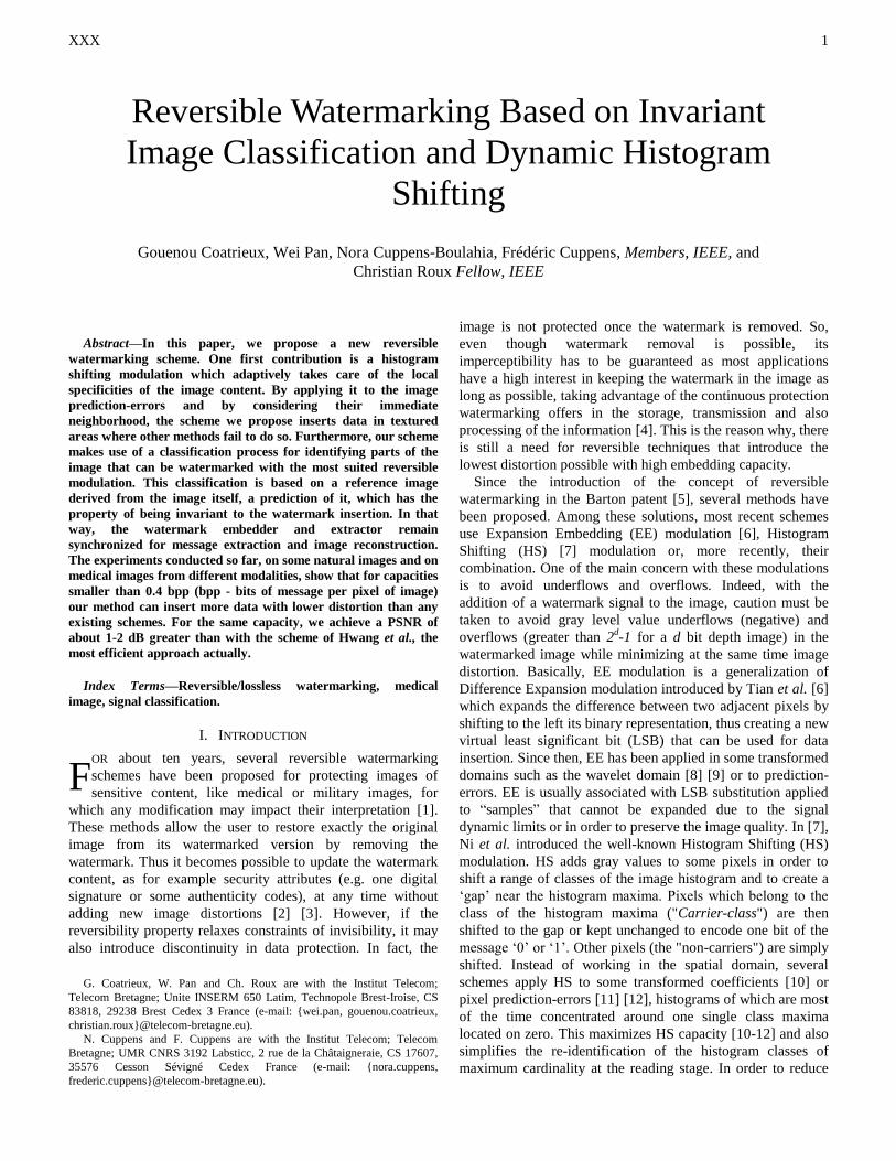
From here on, we work with the image prediction-error.

Considering the pixel block in Fig. 2, the prediction-error ei,j

of the pixel pi,j is given by jijiji ppe ,,,

ˆ , where jip ,ˆ is the

predicted value of pi,j derived as in [11] [12] from its four

nearest neighbor pixels :

4ˆ1,,11,,1, jijijijiji ppppp (2)

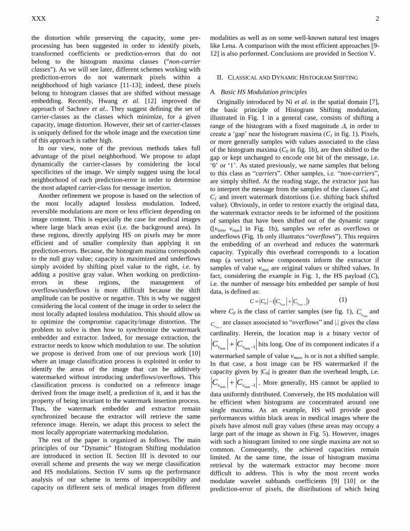
The prediction-error can thus be HS modulated as illustrated

in Fig. 3a. In that case, prediction-errors which do not belong

to the carrier-class Cc = [-∆, ∆[ are considered as “non-

carriers” and are shifted of +/- depending on their sign (+ if

0, jie ; - if 0, jie ). Prediction-errors within the class

Cc = [-∆, ∆[, the “carriers”, are used for embedding. jie , is left

unchanged to encode ‘0’ or shifted to the range [-2∆, -∆[ or [∆,

2∆[, depending on its sign, to encode ‘1’. Notice that, even

though message insertion is conducted in the prediction-error,

it is the image pixels which are modulated. As a consequence,

overflows and underflows appear in the spatial domain. It must

be known, even though this is quite rare, that

overflows/underflows may also appear in the prediction-error

domain, for instance when the image is saturated by noise.

From this standpoint, different refinements have been

proposed in order to optimize capacity and minimize

distortion. Instead of simply shifting by ∆ carrier prediction-

errors, some authors apply EE modulation to them (see Section

I). We do not have space to go into details, but this process

results in adapting the shifting amplitude to the prediction-

error value instead of shifting all of them by a constant ∆. The

capacity is identical but distortion is minimized. Sachnev et al.

[11] as well as Hwang et al. [12] and some others [14] [15]

take advantage of this refinement. Our scheme does not, even

though it can. Distortion can also be minimized by avoiding

shifting non-carrier prediction-errors. As stated earlier, these

prediction-errors belong to blocks of high variance, i.e. blocks

where the predictor bias is high. Recently, Hwang et al. [12]

extended the scheme of Sachnev et al. [11] by looking

iteratively for the frontiers between the carrier-classes and

non-carrier classes so as to minimize image distortion at a

given capacity rate. By doing so, they achieve the best

performance reported so far.

B. Dynamic histogram shifting

As stated above, prediction-errors that encode the message

belong to the carrier-class Cc = [-∆, ∆[, other prediction-errors

are non-carriers. This predicate is static for the whole image

and does not consider the local specificities of the image

signal. Moreover, because prediction acts as a low-pass filter,

most prediction-error carriers are located within smooth image

regions. Highly textured regions contain non-carriers. The

basic idea of our proposal is thus to gain carriers in such a

region by adapting the carrier-class Cc depending on the local

context of the pixel or of the prediction-error to be

watermarked. We propose a Dynamic Histogram Shifting

modulation to achieve this goal.

Let us consider the dashed pixel block B in Fig. 2. Let us

also assume that we aim only at modulating the prediction-

errors ei,j (or equivalently pi,j) indicated by 'x' in Fig.2, leaving

intact their immediate neighborhood. Because of the local

Fig.3. HS modulation applied on predict errors: (a) classical modulation;

(b) dynamical modulation

Fig.2. Pixel neighborhood for prediction – in a 3x3 pixels block B, pi,j is

estimated through its four nearest neighbors pi-1,j, pi,j+1, pi+1,j and pi,j-1.

C0 C1 C2 C3 C4 C5

|Ck|

Classes C0 C1 C2 C3 C4 C5

|Ck|

Classes

+

‘0’ ‘1’

Overflows +

Carriers

Non Carriers

(a) (b)

Fig.1. Histogram shifting modulation. (a) original histogram (b) histogram

of the watermarked data.

XXX 4

stationarity of the image signal we can assume without too

much risk that contiguous prediction-errors have the same

behavior. As a consequence, we suggest considering the

prediction-error neighborhood so as to better define the

location of Cc on the prediction-error dynamic.

Taking the eight neighbors of pi,j: {pi-k,j-l}k,l =-1 …1, we can get

their respective prediction-errors ei-k,j-l. We propose then to

define the carrier-class Cc as the histogram range to which the

absolute values of prediction-errors {|ei-k,j-l|}k,l =-1 ..1, k,l≠0,0

belong (see Fig.3b): Cc = [-me-∆/2, -me+∆/2[[me-∆/2,

me+∆/2[, where me is the mean-value of {|ei-k,j-l|} k,l =-1 ..1, k,l≠0,0.

Our choice in using the absolute value instead of using the

prediction-error itself stands in the fact that contiguous

prediction-errors are distributed around the zero value. Using

their mean-value or a linear combination of them will result in

predicting Cc centered on zero. Based on our approach, the

reference class Cc is determined dynamically for each

prediction-error of the image. In fact, it allows us to

compensate the prediction-error in textured regions and

consequently gives us the capability to insert data in such areas

where other methods fail to do so.

It is important to notice that pi,j as well as all pixels

identified by ‘x’ in Fig.2 are modified after embedding. As a

consequence, the prediction-error neighborhood of pi,j will

also vary if it is computed based on eq. 2. The solution we

adopted to overcome this issue consists to use the predicted-

value jip ,ˆ instead of pi,j in eq. 2. For example, the prediction-

error ei-1,j is given by jijiji ppe ,1,1,1

ˆ

with

4ˆˆˆ1,1,1,1,2,1 jijijijiji ppppp . pi-2,j and pi,j are

replaced by their predicted-value respectively. This means that

the prediction-error neighborhood is not derived from the

original image but from a copy of it where pixels for

embedding are replaced by their predicted-values. An

alternative to this strategy is to compute the prediction-error

neighborhood using the diagonal pixel neighbors. However,

this later approach appears to be less efficient.

As exposed, with our strategy, the location of Cc is

computed independently of ei,j, (or equivalently of pi,j,), and

will be retrieved by the extractor: embedder and extractor

remain synchronized without having to embed some extra-

overhead. Nevertheless, our dynamic histogram shifting

modulation requires performing the watermarking of the image

in several passes. Herein, one quarter of the image pixels are

watermarked at each pass in order to ensure that their

prediction-error neighborhood remains unchanged (see Fig. 2).

Going through the image into several passes in order to

watermark all the pixels is not new. This is the case of most

methods working with HS applied to pixel prediction-errors

[11][12].

The modulation we propose provides no advantage

regarding overflows/underflows which still have to be

managed. We come back to this issue in the next section where

we proposed an original strategy for that purpose.

Let us also notice that, as for any HS modulations (see

section II-A), one can gain in performance by applying EE

modulation on the prediction-error carriers instead of simply

shifting them. For the same capacity, the distortion will be

reduced. The scheme we present thereafter does not use EE.

As a consequence, the performance we give in section IV can

be improved.

III. PROPOSED SCHEME

As mentioned previously, our scheme relies on two main

steps. The first one corresponds to an "invariant" classification

process for the purpose of identifying different sets of image

regions. These regions are then independently watermarked

taking advantage of the most appropriate HS modulation.

From here on, we decided distinguishing two regions where

HS is directly applied to the pixels or applied dynamically to

pixel prediction-errors respectively. We will refer the former

modulation as PHS (for "Pixel Histogram Shifting") and the

later as DPEHS (for "Dynamic Prediction-Error Histogram

Shifting"). Our choice is based on our medical image data set,

for which PHS may be more efficient and simple than the

DPEHS in the image black background, while DPEHS will be

better within regions where the signal is non-null and textured

(e.g. the anatomical object). In the next section we introduce

the basic concept of the invariance property of our

classification process before detailing how it interacts with

PHS and DPEHS. We also introduce some constraints we

imposed on DPEHS in order to minimize image distortion and

then present the overall procedure our scheme follows.

A. Invariant image classification

As said above, our classification process exploits a

reference image I derived from the image I itself under the

two following constraints : i) I remains unchanged after I has

been watermarked into Iw, i.e. I and Iw have the same reference

image; ii) I keeps the properties of an image signal so as to

serve a classification process.

Even though PHS and DPEHS only modulate one pixel

value within one block of the image (see section II-B and

Fig.2), let us consider a more general framework where we

watermark Bk, the k

th block of the image, by adding or

subtracting a watermark pattern W, i.e. Bkw = B

k +/- W. In our

classification process, we associate the reference block

k

NjNi

k

NjNi

k

ji

k pppB ,,,ˆ,...,ˆ,ˆˆ to

k

NjNi

k

NjNi

k

ji

k pppB ,,, ,...,, . Considering linear

algebra, the invariance constraint can be expressed as kB = A.

kB =A. k

wB =A.(kB +/-W) (3)

where A is matrix of (2N+1)x(2N+1) coefficients for a block of

(2N+1)x(2N+1) pixels. As defined, W is in the null space of A.

At the same time, in order to ensure that kB keeps the signal

properties of an image, it can be designed as a predicted

version or a low pass filtered version of B.

To exemplify this, let us consider again the 3x3 pixel block

as illustrated in fig. 2, and the watermark pattern W=[ 1, 0, 0,

0, 0, 0, 0, 0, 0]. In fact, W is added or subtracted so as to apply

PHS or DPEHS (see sections II-A and II-B). In that case, the

corresponding matrix A is given by: kk BAB .ˆ (4)

XXX 5

k

ji

k

ji

k

ji

k

ji

k

ji

k

ji

k

ji

k

ji

k

ji

k

ji

k

ji

k

ji

k

ji

k

ji

k

ji

k

ji

k

ji

k

ji

p

p

p

p

p

p

p

p

p

p

p

p

p

p

p

p

p

p

1,1

,1

1,1

1,

1,

1,1

,1

1,1

,

1,1

,1

1,1

1,

1,

1,1

,1

1,1

,

10000000001000000000100000000010000000001000000000100000000010000000001004/104/14/104/100

ˆ

ˆ

ˆ

ˆ

ˆ

ˆ

ˆ

ˆ

ˆ

(5)

The reference block of Bk corresponds then to

k

ji

k

ji

k

ji

k pppB 1,11,1, ,...,,ˆˆ where

k

jip ,ˆ is a linear

combination of k

jip , .

Once these constraints are fulfilled, the watermark extractor

will retrieve exactly I . Beyond, this allows us to characterize

each block of the image by some simple measures extracted

from its block of reference (e.g. maximum and minimum

values, mean or standard deviation and so on). Such a block

characterization is the basis of our classification process.

To illustrate this purpose, let us consider the first

classification process whose objective for medical images is to

discriminate regions that will be PHS or DPEHS watermarked.

As stated, this corresponds merely distinguishing the black

background of the image from the anatomical object. Let us

continue also with the application matrix A in eq. 5. In order to

decide if one block Bk belongs to the background or not, one

can simply characterizes Bk by its value jip ,

ˆ (issued from kB )

and compare it to a threshold so as to take a decision. In our

implementation, based on the fact that PHS and DPEHS are

parameterized by a shift of magnitude Δ, we fixed this

threshold equal to Δ, i.e. if jip ,ˆ < Δ then kB belongs to the

PHS region otherwise to the DPEHS region. From here on, we

will also consider as part of the image background, blocks

satisfying jip ,ˆ > (2

d-1) – Δ (for a d bit depth image). The

reason is because the medical image background sometimes

contains saturated pixels corresponding to some annotations or

markers that indicate, for example, the image acquisition

orientation (e.g. right or left).

From that standpoint, we can distinguish different parts of

the image and the extractor will be able to retrieve them easily

if it knows A. Our scheme uses this approach not only for

identifying image regions where to apply PHS or DPEHS but

also for managing underflows and overflows, i.e. we do not

have to watermark some extra-overhead data. We come back

to this issue in the next section.

Notice also that the structure of the watermark pattern W

can be made more complex. In fact, it depends on the insertion

modulation. In [10], we carried out the embedding in the Haar

wavelet transform of 2x2 pixel blocks considering a pattern W

such as W=[1, -1, -1, 1].

B. Management of underflows/overflows

For sake of simplicity, let us consider one quarter of the

image pixels for message embedding, i.e. the pixels indicated

by ‘x’ in Fig. 2. Let us also consider a specific run into the

image and note pk the k

th pixel considered for embedding.

Each pixel pk can be framed by a block B

k of 3x3 pixels – see

dashed block in Fig.2 – to which is associated a reference

block k

ji

k

ji

k

ji

k pppB 1,11,1, ,...,,ˆˆ computed using the

matrix A in eq. 5 (k

jip ,ˆ is a linear prediction of

k

jip , ). k

jip ,

will be PHS or DPEHS modulated. This can be viewed as the

addition or subtraction of watermark pattern W to the block Bk,

where W=[ 1, 0, 0, 0, 0, 0, 0, 0, 0] (see above). As a

consequence, despite the fact there is a block overlap,

reference blocks remain invariant to the insertion process.

PHS underflows/overflows

According to the previous classification, PHS is applied to a

pixel k

jip , if its predicted-value falls in the range identified by

jikp ,ˆ < Δ (low-part) and ji

kp ,ˆ > (2d-1) – Δ (high-part). Because

in the low-part (resp. high-part), PHS shifts the pixels by

adding (resp. subtracting) Δ gray values; there is no risk of

underflow (resp. overflow). However, the risk an overflow

(resp. underflow) occurs is not null. It happens when jikp ,ˆ < Δ

(resp. jikp ,ˆ > (2

d-1) – Δ) while pi,j>(2

d-1) – Δ (resp. pi,j< Δ), it

means when the pixel in the center of the block is completely

different from its neighbors. Based on the fact that the image

signal is usually highly correlated locally and that Δ

corresponds to a few number of gray levels, these overflows

(resp. underflows) are unlikely to happen. Even though such

an overflow or underflow never occurred in all the

experiments we conducted so far, our system handles this

situation. It embeds along with the message an overhead

constituted of two flags indicating an overflow and/or an

underflow occurred followed by the necessary information for

restoring the image pixels (see section II.A).

DPEHS underflows/overflows

By definition (see section II-B), DPEHS results in

adding/subtracting Δ to k

jip , (or adding/subtracting W to kB ) in

order to modulate its prediction-error. Hence, some pixels may

lead to an underflow/overflow if watermarked. To distinguish

“watermarkable” pixels (or blocks), i.e. pixels that do not

introduce overflow or underflow if modified, we propose a

second classification process also based on the reference

image I , or more precisely on the reference block kB .

In order to build up this classification process we propose to

characterize one pixel k

jip , (or equivalently its framed block

Bk) through some characteristics extracted from its reference

block ˆ kB . The objective is to discriminate watermarkable

pixels (or blocks) from the others with these characteristics.

Herein, two characteristics are used. They are defined as kBmin

ˆ and kBmaxˆ and correspond to the minimum and maximum

values of ˆ kB respectively. Then, considering in the image the

No and Nu pixels (or equivalently blocks) that if watermarked

by adding or subtracting Δ to k

jip , (or by adding/subtracting

XXX 6

W to Bk) lead to an overflow or and underflow respectively, we

can identify two thresholds Tmin and Tmax such as

Tmin = max n=1..Nu (nBmin

ˆ ); Tmax = min m=1..No (mBmax

ˆ ) (6)

A block Bk or its corresponding pixel p

ki,j is then considered as

watermarkable if it satisfies the following constraints: kBmin

ˆ > Tmin and kBmaxˆ < Tmax (7)

otherwise, it is considered as non-watermarkable and will not

be modified. More clearly, we do not watermark pixels (or

blocks) of same characteristics than those subject to overflows

or underflows if watermarked. Notice that this classification

process is done before DPEHS message insertion is conducted.

Indeed we need to know which pixels are watermarkable.

Following the same strategy, conducted on some invariant

characteristics, the extractor will re-identify non-

watermarkable pixels from the others. Nevertheless, in some

cases, the extractor can identify threshold values Trmin and T

rmax

different from Tmin and Tmax computed at the embedding stage.

In fact, some watermarked pixels (or blocks) may be identified

by the extractor as subject to underflow or overflow changing

at the same time the threshold values in a way such as

Trmin>Tmin and T

rmax<Tmax. If this change occurs the extractor

needs to be informed of the original values of Tmin and Tmax so

as to retrieve all watermarked pixels and recover the original

image perfectly. In our system, flag bits that indicate the

change of Tmin and Tmax as well as their original values are

embedded along with the message and a two step insertion

process is used. During the first step, Tmin and Tmax and a part

of the message is embedded considering the values of Trmin and

Trmax the decoder will find. The remaining portion of the

message is embedded by modifying the last watermarkable

pixels. On the recipient side, the extractor will extract the first

part of the message based on Trmin and T

rmax. It will get access

to the rest of the information after a second reading step.

The way we manage threshold changes is based on the fact

the embedder knows exactly what the extractor will see

applying the same strategy. Thus, after having watermarked a

pixel, the embedder checks if this one will be subject to an

overflow or underflow from the extractor point of view and if

it changes the threshold values. Most of the time, the change of

Tmin or Tmax into Trmin or T

rmax respectively is due to one non-

carrier pixel (i.e. one pixel associated to one non-carrier

prediction-error). The embedder can easily identify such a

pixel as it can only be modified in one way (adding or

subtracting Δ - see section II.B). Then, informed by a flag bit

the embedder has inserted along with the message, the

extractor knows that Trmin and/or T

rmax differ from Tmin and/or

Tmax respectively and it has some other blocks to read and

restore. Nevertheless, for some images, the change can occur

on a carrier prediction-error. This situation is more difficult to

handle as the pixel modification depends on the bit value of

the message to be embedded (see section II-A). More clearly,

depending if the bit value to embed is equal to ‘0’ or ‘1’, the

threshold change may occur or not. To overcome this problem,

we decided to embed in the pixel the bit value that causes the

threshold change and to inform the extractor of that situation

by inserting another flag bit set to 1 along with the message. At

the decoding stage, the extractor knows that the change occurs

on a carrier prediction-error and will not consider the

embedded bit as part of the message. It will restore such a

pixel according to this rule.

To summarize, the DPEHS overhead contains: four flag bits

indicating if Trmin ≠ Tmin and T

rmax ≠ Tmax and if the change

occurs or not on carrier prediction-error. If necessary, Tmin

or/and Tmax are also encoded in the overhead. Thus, our

overhead is of very small size. This contributes to the better

performance of our system in terms of capacity.

C. DPEHS and distortion minimization

In order to minimize the distortion, we also propose two

other refinements or constraints to be satisfied by DPEHS

watermarkable pixels (or blocks). Firstly, like Sachnev et al.

and some others [11] [13], we do not watermark blocks or

pixels of too large estimator biases. These pixels belong to

highly textured blocks. They can be identified through the

standard deviation from their block of reference. Thus pki,j (or

Bk) is watermarkable if it also satisfies

k

stdB < Tstd (8)

where k

stdB is the standard deviation of ˆ kB and Tstd is a

threshold we define in this study as the standard deviation

mean of all reference blocks. Contrary to Sachnev et al. [11]

and others [13], our extractor will retrieve Tstd, computing it by

itself, and will achieve the same classification.

Along the same line, we do not DPEHS watermark blocks

which carrier-class Cc cannot be identified accurately. These

blocks are characterized by a prediction-error neighborhood of

high standard deviation k

stde . Thus pki,j is modified if

k

stde < Te (9)

where Te corresponds to the mean of {k

stde } over the whole

image. It is important to notice that, the prediction-error

neighborhood considered here is the same as in section II-B.

This one is computed replacing in eq. 2 the value of pixels

considered for embedding by their predicted values.

D. Overall scheme

To sum up, our algorithm runs through the image between

one and four times. Each embedding pass is conducted

independently from the other on one quarter of the image

pixels considering the following procedure:

1. Considering a specific run into the image, possibly based

on a secret key, pixels are classified into PHS region or

DPEHS region. For that purpose, pixels are estimated

using eq. 2.

2. One part of the message is embedded in the PHS region

along with some overhead in case of

overflows/underflows (see section III.B).

3. The rest of the message is embedded into the pixels of the

DEPHS region according the following steps:

a. Step 1: as depicted in section III.B, the classification

thresholds Tmin and Tmax are computed in order to

discriminate watermarkable pixels from the others. At

the same time the embedder verifies if the extractor will

find or not the same thresholds. For that purpose, the

XXX 7

watermark W=[ 1, 0, 0, 0, 0, 0, 0, 0, 0] is considered

while each pixel is associated with a reference block of

3x3 pixels using the matrix A (see section III.B). Pixel

prediction-errors as well as prediction-error

neighborhoods are also computed (see section II-B).

This information is necessary to the embedder so as to

manage threshold changes (i.e. to know if the changes

occur on a carrier prediction-error or a non-carrier

prediction-error). At the end of this process, the

embedder builds the message overhead (flags

concatenated with the values of Tmin and Tmax in case

Trmin ≠ Tmin and T

rmax ≠ Tmax) and computes the

thresholds Tstd and Te (see section III.C).

b. Step 2: message embedding is conducted in one or two

stages depending if Trmin ≠ Tmin and T

rmax ≠ Tmax and

on the value of Tstd and Te.

At the reading stage, in the case the matrix A is predefined,

the only parameter the extractor needs to know is the

histogram shifting amplitude Δ which parameterizes PHS and

DPEHS as well as the classification processes (see sections

III.A and III.B). Notice that in this scheme, the value of Δ is

fixed by the user. Message extraction is conducted

independently in each region and pass. For the DPEHS

message, the extractor will retrieve by itself the values of Tmin,

Tmax, Tstd and Te and will apply or not a two-stage message

extraction process (see section III.B).

IV. EXPERIMENTS

A. Image database and measures of performance

The previous watermarking scheme has been tested and

compared with some recent methods [9-12]. All have been

applied to several natural grayscale images (like Lena and

Baboon (see Fig. 4), used as reference in the literature), and

different series of medical images issued from five distinct

modalities. These image sets, illustrated in Fig. 5, contain

respectively:

three 12 bit encoded Magnetic Resonance Image (MRI)

volumes of 79, 80 and 99 axial slices of 256x256 pixels

respectively;

three 16 bit encoded Positron Emission Tomography

(PET) volumes of 234, 213 and 212 axial slices of

144x144 pixels respectively;

three sequences of 8 bit encoded Ultrasound (US) images.

The first sequence contains 14 images of 480x592 pixels,

and the two others 9 and 30 images of 480x472 pixels

respectively;

forty two 12 bit encoded X-ray images of 2446x2010

pixels, and;

thirty 8 bit encoded retina images of 1008x1280 pixels.

To objectively quantify achieved performance, different

criteria have been considered:

- the capacity rate C expressed in bpp (bit of message per

pixel of image);

- and, the Peak Signal to Noise Ratio (PSNR) so as to

measure the distortion between an image I and its

watermarked version Iw

),,

12(log10

,

1,1,

2

2

10

MN

ji w

d

jiIjiI

NMPSNR (10)

where d corresponds to the image depth and N and M to

the image dimensions.

In the following experiments, the embedded message is a

binary sequence randomly generated according to a uniform

distribution.

B. Experimental results

Results are given in Tables I-III and in Fig. 6 in terms of

capacity and image distortion depending on: the pixel shifting

magnitude ∆ (see section II); and the number of times our

algorithm goes through the image (between 1 and 4 times, see

previous section).

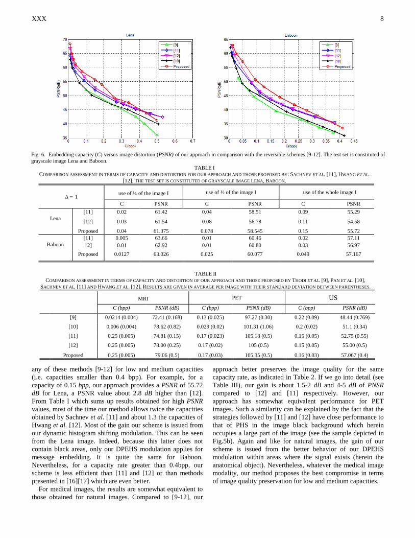
Results for natural images are given in Table I and Fig.6,

where we compare our technique with the four other schemes

proposed in [9-12]. Presented curves have been obtained

making varying ∆ and the number of embedding passes

progressively. Notice that the method of Hwang et al. [12],

derived from the scheme of Sachnev et al. [11], is actually the

best algorithm reported today. As can be seen from Fig. 6, our

method provides a better capacity/distortion compromise than

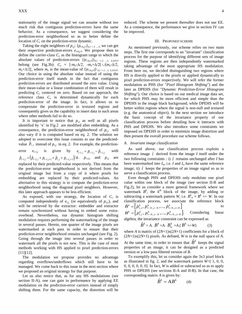
(a) (b) (c) (d) (e)

Fig. 5. Image samples from our different medical image test sets: (a) 12 bit encoded MRI axial slice of the head of 256x256 pixels; (b) 16 bit encoded PET

image of 144x144 pixels; (c) 8 bit encoded ultrasound image of 480x592 pixels,; (d) 12 bit encoded X-ray image of 2446x2010 pixels; (e) 8 bit encoded

retina image of 1008x1280 pixels.

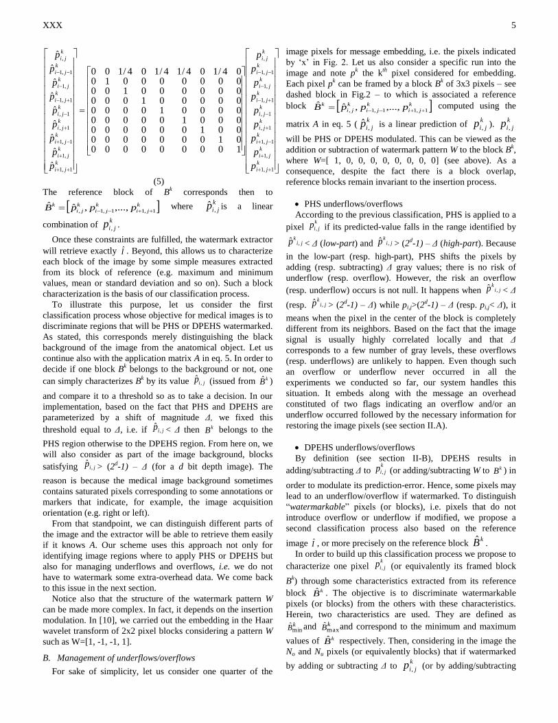
(a) (b)

Fig. 4. Natural test images, grayscale images of 512x512 pixels: (a)

Lena, (b) Baboon.

XXX 8

any of these methods [9-12] for low and medium capacities

(i.e. capacities smaller than 0.4 bpp). For example, for a

capacity of 0.15 bpp, our approach provides a PSNR of 55.72

dB for Lena, a PSNR value about 2.8 dB higher than [12].

From Table I which sums up results obtained for high PSNR

values, most of the time our method allows twice the capacities

obtained by Sachnev et al. [11] and about 1.3 the capacities of

Hwang et al. [12]. Most of the gain our scheme is issued from

our dynamic histogram shifting modulation. This can be seen

from the Lena image. Indeed, because this latter does not

contain black areas, only our DPEHS modulation applies for

message embedding. It is quite the same for Baboon.

Nevertheless, for a capacity rate greater than 0.4bpp, our

scheme is less efficient than [11] and [12] or than methods

presented in [16][17] which are even better.

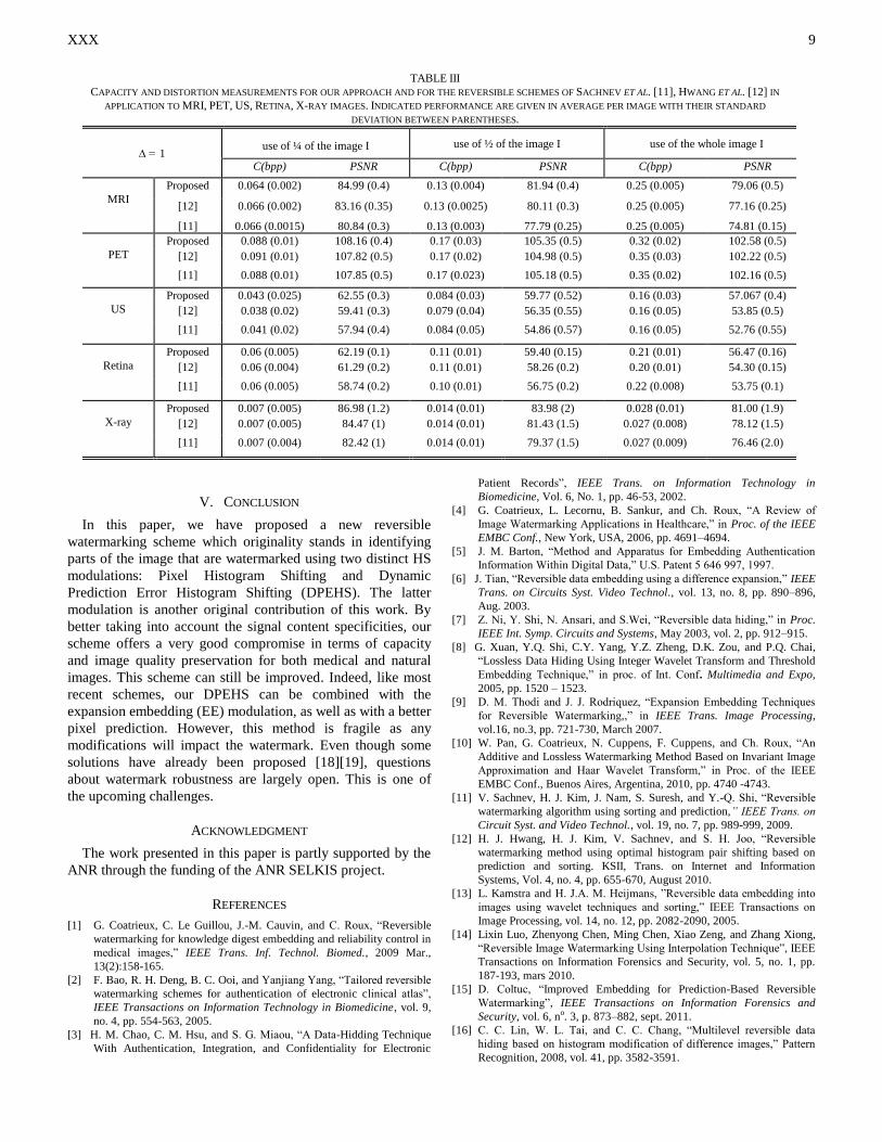
For medical images, the results are somewhat equivalent to

those obtained for natural images. Compared to [9-12], our

approach better preserves the image quality for the same

capacity rate, as indicated in Table 2. If we go into detail (see

Table III), our gain is about 1.5-2 dB and 4-5 dB of PNSR

compared to [12] and [11] respectively. However, our

approach has somewhat equivalent performance for PET

images. Such a similarity can be explained by the fact that the

strategies followed by [11] and [12] have close performance to

that of PHS in the image black background which herein

occupies a large part of the image (see the sample depicted in

Fig.5b). Again and like for natural images, the gain of our

scheme is issued from the better behavior of our DPEHS

modulation within areas where the signal exists (herein the

anatomical object). Nevertheless, whatever the medical image

modality, our method proposes the best compromise in terms

of image quality preservation for low and medium capacities.

Fig. 6. Embedding capacity (C) versus image distortion (PSNR) of our approach in comparison with the reversible schemes [9-12]. The test set is constituted of

grayscale image Lena and Baboon.

TABLE I

COMPARISON ASSESSMENT IN TERMS OF CAPACITY AND DISTORTION FOR OUR APPROACH AND THOSE PROPOSED BY: SACHNEV ET AL. [11], HWANG ET AL.

[12]. THE TEST SET IS CONSTITUTED OF GRAYSCALE IMAGE LENA, BABOON.

∆ = 1 use of ¼ of the image I use of ½ of the image I use of the whole image I

C PSNR C PSNR C PSNR

Lena

[11] 0.02 61.42 0.04 58.51 0.09 55.29

[12] 0.03 61.54 0.08 56.78 0.11 54.58

Proposed 0.04 61.375 0.078 58.545 0.15 55.72

Baboon

[11] 0.005 63.66 0.01 60.46 0.02 57.11

12] 0.01 62.92 0.01 60.80 0.03 56.97

Proposed 0.0127 63.026 0.025 60.077 0.049 57.167

TABLE II

COMPARISON ASSESSMENT IN TERMS OF CAPACITY AND DISTORTION OF OUR APPROACH AND THOSE PROPOSED BY THODI ET AL. [9], PAN ET AL. [10],

SACHNEV ET AL. [11] AND HWANG ET AL. [12]. RESULTS ARE GIVEN IN AVERAGE PER IMAGE WITH THEIR STANDARD DEVIATION BETWEEN PARENTHESES.

MRI PET US

C (bpp) PSNR (dB) C (bpp) PSNR (dB) C (bpp) PSNR (dB)

[9] 0.0214 (0.004) 72.41 (0.168) 0.13 (0.025) 97.27 (0.30) 0.22 (0.09) 48.44 (0.769)

[10] 0.006 (0.004) 78.62 (0.82) 0.029 (0.02) 101.31 (1.06) 0.2 (0.02) 51.1 (0.34)

[11] 0.25 (0.005) 74.81 (0.15) 0.17 (0.023) 105.18 (0.5) 0.15 (0.05) 52.75 (0.55)

[12] 0.25 (0.005) 78.00 (0.25) 0.17 (0.02) 105 (0.5) 0.15 (0.05) 55.00 (0.5)

Proposed 0.25 (0.005) 79.06 (0.5) 0.17 (0.03) 105.35 (0.5) 0.16 (0.03) 57.067 (0.4)

XXX 9

V. CONCLUSION

In this paper, we have proposed a new reversible

watermarking scheme which originality stands in identifying

parts of the image that are watermarked using two distinct HS

modulations: Pixel Histogram Shifting and Dynamic

Prediction Error Histogram Shifting (DPEHS). The latter

modulation is another original contribution of this work. By

better taking into account the signal content specificities, our

scheme offers a very good compromise in terms of capacity

and image quality preservation for both medical and natural

images. This scheme can still be improved. Indeed, like most

recent schemes, our DPEHS can be combined with the

expansion embedding (EE) modulation, as well as with a better

pixel prediction. However, this method is fragile as any

modifications will impact the watermark. Even though some

solutions have already been proposed [18][19], questions

about watermark robustness are largely open. This is one of

the upcoming challenges.

ACKNOWLEDGMENT

The work presented in this paper is partly supported by the

ANR through the funding of the ANR SELKIS project.

REFERENCES

[1] G. Coatrieux, C. Le Guillou, J.-M. Cauvin, and C. Roux, “Reversible

watermarking for knowledge digest embedding and reliability control in

medical images,” IEEE Trans. Inf. Technol. Biomed., 2009 Mar.,

13(2):158-165.

[2] F. Bao, R. H. Deng, B. C. Ooi, and Yanjiang Yang, “Tailored reversible

watermarking schemes for authentication of electronic clinical atlas”,

IEEE Transactions on Information Technology in Biomedicine, vol. 9,

no. 4, pp. 554-563, 2005.

[3] H. M. Chao, C. M. Hsu, and S. G. Miaou, “A Data-Hidding Technique

With Authentication, Integration, and Confidentiality for Electronic

Patient Records”, IEEE Trans. on Information Technology in

Biomedicine, Vol. 6, No. 1, pp. 46-53, 2002.

[4] G. Coatrieux, L. Lecornu, B. Sankur, and Ch. Roux, “A Review of

Image Watermarking Applications in Healthcare,” in Proc. of the IEEE

EMBC Conf., New York, USA, 2006, pp. 4691–4694.

[5] J. M. Barton, “Method and Apparatus for Embedding Authentication

Information Within Digital Data,” U.S. Patent 5 646 997, 1997.

[6] J. Tian, “Reversible data embedding using a difference expansion,” IEEE

Trans. on Circuits Syst. Video Technol., vol. 13, no. 8, pp. 890–896,

Aug. 2003.

[7] Z. Ni, Y. Shi, N. Ansari, and S.Wei, “Reversible data hiding,” in Proc.

IEEE Int. Symp. Circuits and Systems, May 2003, vol. 2, pp. 912–915.

[8] G. Xuan, Y.Q. Shi, C.Y. Yang, Y.Z. Zheng, D.K. Zou, and P.Q. Chai,

“Lossless Data Hiding Using Integer Wavelet Transform and Threshold

Embedding Technique,” in proc. of Int. Conf. Multimedia and Expo,

2005, pp. 1520 – 1523.

[9] D. M. Thodi and J. J. Rodriquez, “Expansion Embedding Techniques

for Reversible Watermarking,,” in IEEE Trans. Image Processing,

vol.16, no.3, pp. 721-730, March 2007.

[10] W. Pan, G. Coatrieux, N. Cuppens, F. Cuppens, and Ch. Roux, “An

Additive and Lossless Watermarking Method Based on Invariant Image

Approximation and Haar Wavelet Transform,” in Proc. of the IEEE

EMBC Conf., Buenos Aires, Argentina, 2010, pp. 4740 -4743.

[11] V. Sachnev, H. J. Kim, J. Nam, S. Suresh, and Y.-Q. Shi, “Reversible

watermarking algorithm using sorting and prediction,” IEEE Trans. on

Circuit Syst. and Video Technol., vol. 19, no. 7, pp. 989-999, 2009.

[12] H. J. Hwang, H. J. Kim, V. Sachnev, and S. H. Joo, “Reversible

watermarking method using optimal histogram pair shifting based on

prediction and sorting. KSII, Trans. on Internet and Information

Systems, Vol. 4, no. 4, pp. 655-670, August 2010.

[13] L. Kamstra and H. J.A. M. Heijmans, ”Reversible data embedding into

images using wavelet techniques and sorting,” IEEE Transactions on

Image Processing, vol. 14, no. 12, pp. 2082-2090, 2005.

[14] Lixin Luo, Zhenyong Chen, Ming Chen, Xiao Zeng, and Zhang Xiong,

“Reversible Image Watermarking Using Interpolation Technique”, IEEE

Transactions on Information Forensics and Security, vol. 5, no. 1, pp.

187-193, mars 2010.

[15] D. Coltuc, “Improved Embedding for Prediction-Based Reversible

Watermarking”, IEEE Transactions on Information Forensics and

Security, vol. 6, no. 3, p. 873–882, sept. 2011.

[16] C. C. Lin, W. L. Tai, and C. C. Chang, “Multilevel reversible data

hiding based on histogram modification of difference images,” Pattern

Recognition, 2008, vol. 41, pp. 3582-3591.

TABLE III

CAPACITY AND DISTORTION MEASUREMENTS FOR OUR APPROACH AND FOR THE REVERSIBLE SCHEMES OF SACHNEV ET AL. [11], HWANG ET AL. [12] IN

APPLICATION TO MRI, PET, US, RETINA, X-RAY IMAGES. INDICATED PERFORMANCE ARE GIVEN IN AVERAGE PER IMAGE WITH THEIR STANDARD

DEVIATION BETWEEN PARENTHESES.

∆ = 1 use of ¼ of the image I use of ½ of the image I use of the whole image I

C(bpp) PSNR C(bpp) PSNR C(bpp) PSNR

MRI

Proposed 0.064 (0.002) 84.99 (0.4) 0.13 (0.004) 81.94 (0.4) 0.25 (0.005) 79.06 (0.5)

[12] 0.066 (0.002) 83.16 (0.35) 0.13 (0.0025) 80.11 (0.3) 0.25 (0.005) 77.16 (0.25)

[11] 0.066 (0.0015) 80.84 (0.3) 0.13 (0.003) 77.79 (0.25) 0.25 (0.005) 74.81 (0.15)

PET

Proposed 0.088 (0.01) 108.16 (0.4) 0.17 (0.03) 105.35 (0.5) 0.32 (0.02) 102.58 (0.5)

[12] 0.091 (0.01) 107.82 (0.5) 0.17 (0.02) 104.98 (0.5) 0.35 (0.03) 102.22 (0.5)

[11] 0.088 (0.01) 107.85 (0.5) 0.17 (0.023) 105.18 (0.5) 0.35 (0.02) 102.16 (0.5)

US

Proposed 0.043 (0.025) 62.55 (0.3) 0.084 (0.03) 59.77 (0.52) 0.16 (0.03) 57.067 (0.4)

[12] 0.038 (0.02) 59.41 (0.3) 0.079 (0.04) 56.35 (0.55) 0.16 (0.05) 53.85 (0.5)

[11] 0.041 (0.02) 57.94 (0.4) 0.084 (0.05) 54.86 (0.57) 0.16 (0.05) 52.76 (0.55)

Retina

Proposed 0.06 (0.005) 62.19 (0.1) 0.11 (0.01) 59.40 (0.15) 0.21 (0.01) 56.47 (0.16)

[12] 0.06 (0.004) 61.29 (0.2) 0.11 (0.01) 58.26 (0.2) 0.20 (0.01) 54.30 (0.15)

[11] 0.06 (0.005) 58.74 (0.2) 0.10 (0.01) 56.75 (0.2) 0.22 (0.008) 53.75 (0.1)

X-ray

Proposed 0.007 (0.005) 86.98 (1.2) 0.014 (0.01) 83.98 (2) 0.028 (0.01) 81.00 (1.9)

[12] 0.007 (0.005) 84.47 (1) 0.014 (0.01) 81.43 (1.5) 0.027 (0.008) 78.12 (1.5)

[11] 0.007 (0.004) 82.42 (1) 0.014 (0.01) 79.37 (1.5) 0.027 (0.009) 76.46 (2.0)

XXX 10

[17] C.H. Yang and M.H. Tsai, “Improving Histogram-based Reversible

Data Hiding by Interleaving Predictions,” IET Image Processing, vol. 4,

no. 4, pp. 223-234, August 2010.

[18] C. De Vleeschouwer, J.-F. Delaigle, and B. Macq, “Circular

interpretation of bijective transformations in lossless watermarking for

media asset management,” Multimedia, IEEE Trans. on, vol. 5, no. 1,

pp. 97– 105, march 2003.

[19] D. Coltuc and J.-M. Chassery, "Distortion-free robust watermarking: a

case study," in Security, Steganography, and Watermarking of

Multimedia Contents IX, San Jose, CA, USA, 2007, pp. 65051N-8.