REVERSIBLE LOGIC SYNTHESIS by DMITRI MASLOV M.Sc. (Mathematics) Lomonosov’s Moscow State University, 1998 MCS University of New Brunswick, 2002 A thesis submitted in partial fulfillment of the requirements for the degree of DOCTOR OF PHILOSOPHY in THE FACULTY OF COMPUTER SCIENCE We accept this thesis as conforming to the required standard ..................................... ..................................... ..................................... ..................................... ..................................... THE UNIVERSITY OF NEW BRUNSWICK September 2003 c “Dmitri Maslov”, 2003

Welcome message from author
This document is posted to help you gain knowledge. Please leave a comment to let me know what you think about it! Share it to your friends and learn new things together.
Transcript
REVERSIBLE LOGIC SYNTHESIS
by
DMITRI MASLOV
M.Sc. (Mathematics) Lomonosov’s Moscow State University, 1998MCS University of New Brunswick, 2002
A thesis submitted in partial fulfillment of
the requirements for the degree of
DOCTOR OF PHILOSOPHY
in
THE FACULTY OF COMPUTER SCIENCE
We accept this thesis as conformingto the required standard
. . . . . . . . . . . . . . . . . . . . . . . . . . . . . . . . . . . . .
. . . . . . . . . . . . . . . . . . . . . . . . . . . . . . . . . . . . .
. . . . . . . . . . . . . . . . . . . . . . . . . . . . . . . . . . . . .
. . . . . . . . . . . . . . . . . . . . . . . . . . . . . . . . . . . . .
. . . . . . . . . . . . . . . . . . . . . . . . . . . . . . . . . . . . .
THE UNIVERSITY OF NEW BRUNSWICK
September 2003
c© “Dmitri Maslov”, 2003

In presenting this thesis in partial fulfillment of the requirements for an advanced degree
at the University of New Brunswick, I agree that the Library shall make it freely available
for reference and study. I further agree that permission for extensive copying of this
thesis for scholarly purposes may be granted by the head of my department or by his
or her representatives. It is understood that copying or publication of this thesis for
financial gain shall not be allowed without my written permission.
(Signature)
Faculty of Computer ScienceThe University of New BrunswickFredericton, Canada
Date
Abstract
Reversible logic is an emerging research area. Interest in reversible logic is sparked by
its applications in several technologies, such as quantum, CMOS, optical and nanotech-
nology. Reversible implementations are also found in thermodynamics and adiabatic
CMOS. Power dissipation in modern technologies is an important issue, and overheat-
ing is a serious concern for both manufacturer (impossibility of introducing new, smaller
scale technologies, limited temperature range for operating the product) and customer
(power supply, which is especially important for mobile systems). One of the main
benefits that reversible logic brings is theoretically zero power dissipation in the sense
that, independently of underlying technology, irreversibility means heat generation.
Most of the listed technologies are either emerging or not fully investigated. As a
result, only a small number of Boolean variables can be computed using hardware
based on reversible technology. Part of this problem comes from the incompleteness of
the technological results, the other part arises from absence of good circuit synthesis
procedures. Synthesis of multiple-output functions has to be done in terms of reversible
objects. This usually results in addition of garbage bits (bits needed for reversibility,
but not required for the output part of a circuit), which in contrast to the non-reversible
case is technologically difficult and expensive. The situation is rather pessimistic when
it is observed that proposed designed synthesis procedures use excessive garbage.
The amount of garbage is a very important criterion for a good synthesis procedure,
since in most technologies the addition of only one bit of garbage is very expensive
or even impossible to implement. Based on this information, a crucial way to help
reversible logic to evolve and become usable is to design a synthesis method which
uses the theoretically minimal number of garbage bits. This will help the emerging
technologies to use the results of reversible synthesis even in the early stage of their
development. Minimal garbage realization may require a larger number of gates in the
circuit, but it is better to have a large but working circuit than a small one that is not
ready for the technology.
In this thesis several synthesis methods that use minimal garbage are considered: RCMG
ii
Abstract
model (defined asa part of this thesis), Toffoli synthesis, Fredkin/Toffoli synthesis. Dy-
namic programming algorithms are synthesized separately with near minimal garbage.
Some of the methods use minimal garbage and produce small circuits (Toffoli and Fred-
kin/Toffoli synthesis) but work with reversible specifications, some handle “don’t cares”
(RCMG), some even allow a trade-off between the garbage amount and the number of
gates in the resulting circuit. When a technology is chosen and the relationship between
costs of one bit of garbage and a single gate is specified, one or the other method may
be better. In the presented thesis the main goal is to design synthesis methods that will
be suitable for different cost distributions.
iii
Acknowledgments
I would like to thank Dr. Marek Perkowski from Portland State University, Oregon, USA
for providing access to his lecture notes on reversible logic and his valuable comments
in the early stages of this research.
Also, I would like to thank Dr. Michael Miller from University of Victoria, Victoria,
Canada for his help and participation in the research done in chapters 4 and 5 while he
was on sabbatical in the University of New Brunswick.
Finally, I would like to thank my scientific advisor Gerhard W. Dueck from University of
New Brunswick, New Brunswick, Canada for his support, help and active participation
in the research.
iv

Glossary
AND — Boolean operation (&, concatenation) with properties 0&0 = 0&1 = 1&0 = 0,
1&1 = 1;
CNOT — Controlled NOT gate, also known as the Feynman gate;
CPU — Central Processing Unit;
EXOR — Boolean operation (⊕) with properties 0 ⊕ 0 = 1 ⊕ 1 = 0, 0 ⊕ 1 = 1 ⊕ 0 = 1;
ESOP — EXOR sum-of-products;
mEXOR — multiple EXOR reversible gates family;
NOT — Boolean operation (¯) with properties 0 = 1, 1 = 0;
PLA — Programmable Logic Array;
RCMG — Reversible Cascades with Minimal Garbage;
RPGA — Reversible Programmable Gate Array.
v
Table of Contents
Abstract ii
Acknowledgments iv
Glossary v
Table of Contents vi
List of Tables viii
List of Figures ix
Chapter 1. Introduction 1
Chapter 2. Basic Definitions and Literature Overview 82.1 Boolean Algebra . . . . . . . . . . . . . . . . . . . . . . . . . . . . . . . . . . . . . . . . . . . . . . . . . . . . . . . . . . 82.2 Basic Definitions of the Reversible Logic . . . . . . . . . . . . . . . . . . . . . . . . . . . . . . . . . 11
2.2.1 Network Structure . . . . . . . . . . . . . . . . . . . . . . . . . . . . . . . . . . . . . . . . . . . . . . . . 132.2.2 The Popular Reversible Gates: Fredkin and Toffoli . . . . . . . . . . . . . . . . 152.2.3 Several Other Reversible Gates . . . . . . . . . . . . . . . . . . . . . . . . . . . . . . . . . . . . 17
2.3 Overview of Reversible Logic Synthesis Methods . . . . . . . . . . . . . . . . . . . . . . . . . 192.4 Related Work . . . . . . . . . . . . . . . . . . . . . . . . . . . . . . . . . . . . . . . . . . . . . . . . . . . . . . . . . . . 24
Chapter 3. Reversible Cascades with Minimal Garbage 263.1 Minimal Garbage . . . . . . . . . . . . . . . . . . . . . . . . . . . . . . . . . . . . . . . . . . . . . . . . . . . . . . . . 28
3.1.1 Analysis of Garbage in Existing Methods . . . . . . . . . . . . . . . . . . . . . . . . . . 293.2 A New Structure: Reversible Cascades with Minimal Garbage . . . . . . . . . . . . 32
3.2.1 Definition of the Model . . . . . . . . . . . . . . . . . . . . . . . . . . . . . . . . . . . . . . . . . . . 323.2.2 Quantum Cost Analysis . . . . . . . . . . . . . . . . . . . . . . . . . . . . . . . . . . . . . . . . . . . 353.2.3 Theoretical Synthesis . . . . . . . . . . . . . . . . . . . . . . . . . . . . . . . . . . . . . . . . . . . . . 38
3.3 Heuristic Synthesis . . . . . . . . . . . . . . . . . . . . . . . . . . . . . . . . . . . . . . . . . . . . . . . . . . . . . . 453.3.1 The Algorithm . . . . . . . . . . . . . . . . . . . . . . . . . . . . . . . . . . . . . . . . . . . . . . . . . . . . 503.3.2 Multiple Output Functions . . . . . . . . . . . . . . . . . . . . . . . . . . . . . . . . . . . . . . . . 523.3.3 Benchmarks . . . . . . . . . . . . . . . . . . . . . . . . . . . . . . . . . . . . . . . . . . . . . . . . . . . . . . 52
3.4 RCMG and ESOP Comparison . . . . . . . . . . . . . . . . . . . . . . . . . . . . . . . . . . . . . . . . . . 573.4.1 Multiple Output Functions . . . . . . . . . . . . . . . . . . . . . . . . . . . . . . . . . . . . . . . . 65
3.5 Conclusions . . . . . . . . . . . . . . . . . . . . . . . . . . . . . . . . . . . . . . . . . . . . . . . . . . . . . . . . . . . . . 65
Chapter 4. Toffoli Synthesis 664.1 The Algorithm . . . . . . . . . . . . . . . . . . . . . . . . . . . . . . . . . . . . . . . . . . . . . . . . . . . . . . . . . . 67
4.1.1 Basic Algorithm . . . . . . . . . . . . . . . . . . . . . . . . . . . . . . . . . . . . . . . . . . . . . . . . . . 674.1.2 Bidirectional Algorithm . . . . . . . . . . . . . . . . . . . . . . . . . . . . . . . . . . . . . . . . . . . 71
4.2 Templates . . . . . . . . . . . . . . . . . . . . . . . . . . . . . . . . . . . . . . . . . . . . . . . . . . . . . . . . . . . . . . . 73
vi
Table of Contents
4.2.1 Unification of Class 1 and Class 2 Templates . . . . . . . . . . . . . . . . . . . . . . 784.3 Templates - a New Approach . . . . . . . . . . . . . . . . . . . . . . . . . . . . . . . . . . . . . . . . . . . . 79
4.3.1 Completeness . . . . . . . . . . . . . . . . . . . . . . . . . . . . . . . . . . . . . . . . . . . . . . . . . . . . . 854.4 Experimental Results . . . . . . . . . . . . . . . . . . . . . . . . . . . . . . . . . . . . . . . . . . . . . . . . . . . . 86
Chapter 5. Toffoli-Fredkin Synthesis 905.1 How Useful Are Fredkin Gates? . . . . . . . . . . . . . . . . . . . . . . . . . . . . . . . . . . . . . . . . . . 905.2 Box Gate . . . . . . . . . . . . . . . . . . . . . . . . . . . . . . . . . . . . . . . . . . . . . . . . . . . . . . . . . . . . . . . . 91
5.2.1 A Note on Similarity of Fredkin And Toffoli Gates . . . . . . . . . . . . . . . . . 935.3 The algorithm . . . . . . . . . . . . . . . . . . . . . . . . . . . . . . . . . . . . . . . . . . . . . . . . . . . . . . . . . . . 94
5.3.1 Handling permutations . . . . . . . . . . . . . . . . . . . . . . . . . . . . . . . . . . . . . . . . . . . 1035.3.2 Multiple output and incompletely specified functions . . . . . . . . . . . . . 104
5.4 Template simplification tool . . . . . . . . . . . . . . . . . . . . . . . . . . . . . . . . . . . . . . . . . . . . 1045.5 Results . . . . . . . . . . . . . . . . . . . . . . . . . . . . . . . . . . . . . . . . . . . . . . . . . . . . . . . . . . . . . . . . . 1115.6 Conclusion . . . . . . . . . . . . . . . . . . . . . . . . . . . . . . . . . . . . . . . . . . . . . . . . . . . . . . . . . . . . . 115
Chapter 6. Asymptotically Optimal Regular Synthesis 1176.1 Quantum Cost of the mEXOR gate . . . . . . . . . . . . . . . . . . . . . . . . . . . . . . . . . . . . . 1186.2 Asymptotically Optimal Reversible Synthesis Method . . . . . . . . . . . . . . . . . . . 1226.3 Conclusion . . . . . . . . . . . . . . . . . . . . . . . . . . . . . . . . . . . . . . . . . . . . . . . . . . . . . . . . . . . . . 127
Chapter 7. Dynamic Programming Algorithms as Reversible Circuits: Sym-metric Function Realization 131
7.1 Application: Multiple Output Symmetric Functions . . . . . . . . . . . . . . . . . . . . . 1337.2 Comparison of the Results . . . . . . . . . . . . . . . . . . . . . . . . . . . . . . . . . . . . . . . . . . . . . . 1397.3 Conclusion . . . . . . . . . . . . . . . . . . . . . . . . . . . . . . . . . . . . . . . . . . . . . . . . . . . . . . . . . . . . . 142
Chapter 8. Summary 143
Chapter 9. Further Research 145
Bibliography 148
vii

List of Tables
2.1 Truth table method . . . . . . . . . . . . . . . . . . . . . . . . . . . . . . . . . . . . . . . . . . . . . . . . . . . . . . . . . 92.2 Truth table for a 3-input 3-output function . . . . . . . . . . . . . . . . . . . . . . . . . . . . . . . . . 102.3 Reversible function computing the logical AND . . . . . . . . . . . . . . . . . . . . . . . . . . . . . 12
3.1 Experimental results . . . . . . . . . . . . . . . . . . . . . . . . . . . . . . . . . . . . . . . . . . . . . . . . . . . . . . . 313.2 Truth table . . . . . . . . . . . . . . . . . . . . . . . . . . . . . . . . . . . . . . . . . . . . . . . . . . . . . . . . . . . . . . . . 343.3 Gate cost comparison . . . . . . . . . . . . . . . . . . . . . . . . . . . . . . . . . . . . . . . . . . . . . . . . . . . . . . 393.4 Truth table of f(x1, x2, x3) = (x1 ⊕ x2x3, x2, x1 ⊕ x2x3) . . . . . . . . . . . . . . . . . . . 463.5 Distance between f and its partial realization . . . . . . . . . . . . . . . . . . . . . . . . . . . . . . 473.6 Effect of changing one bit . . . . . . . . . . . . . . . . . . . . . . . . . . . . . . . . . . . . . . . . . . . . . . . . . . 493.7 Comparison with Miller’s results . . . . . . . . . . . . . . . . . . . . . . . . . . . . . . . . . . . . . . . . . . . 543.8 Comparison with Perkowski’s results . . . . . . . . . . . . . . . . . . . . . . . . . . . . . . . . . . . . . . . 553.9 Comparison with Khan’s results . . . . . . . . . . . . . . . . . . . . . . . . . . . . . . . . . . . . . . . . . . . . 563.10 Complexity of the function exphardn. . . . . . . . . . . . . . . . . . . . . . . . . . . . . . . . . . . . . . . 64
4.1 Example of applying the basic algorithm. . . . . . . . . . . . . . . . . . . . . . . . . . . . . . . . . . . 694.2 Example of applying the bidirectional algorithm. . . . . . . . . . . . . . . . . . . . . . . . . . . . 734.3 Second gate building process . . . . . . . . . . . . . . . . . . . . . . . . . . . . . . . . . . . . . . . . . . . . . . . 79
5.1 Optimal synthesis of all 3-input 3-output functions . . . . . . . . . . . . . . . . . . . . . . . . . 915.2 Basic approach synthesis. . . . . . . . . . . . . . . . . . . . . . . . . . . . . . . . . . . . . . . . . . . . . . . . . . 1015.3 Bidirectional approach synthesis. . . . . . . . . . . . . . . . . . . . . . . . . . . . . . . . . . . . . . . . . . . 1035.4 Results . . . . . . . . . . . . . . . . . . . . . . . . . . . . . . . . . . . . . . . . . . . . . . . . . . . . . . . . . . . . . . . . . . . 115
6.1 Cost comparison. . . . . . . . . . . . . . . . . . . . . . . . . . . . . . . . . . . . . . . . . . . . . . . . . . . . . . . . . . 1216.2 Circuit building process for a four variable function. . . . . . . . . . . . . . . . . . . . . . . . 1296.3 Circuit for the basic approach. . . . . . . . . . . . . . . . . . . . . . . . . . . . . . . . . . . . . . . . . . . . . 130
7.1 Comparison of the results to RWC, KGF and GT . . . . . . . . . . . . . . . . . . . . . . . . . 140
viii
List of Figures
2.1 The general structure for a network . . . . . . . . . . . . . . . . . . . . . . . . . . . . . . . . . . . . . . . . 142.2 NOT, CNOT and Toffoli gates . . . . . . . . . . . . . . . . . . . . . . . . . . . . . . . . . . . . . . . . . . . . . 162.3 SWAP gate realization in quantum technology . . . . . . . . . . . . . . . . . . . . . . . . . . . . . 17
3.1 Reversible design methods . . . . . . . . . . . . . . . . . . . . . . . . . . . . . . . . . . . . . . . . . . . . . . . . . 303.2 Horizontal line types. . . . . . . . . . . . . . . . . . . . . . . . . . . . . . . . . . . . . . . . . . . . . . . . . . . . . . . 323.3 A single gate . . . . . . . . . . . . . . . . . . . . . . . . . . . . . . . . . . . . . . . . . . . . . . . . . . . . . . . . . . . . . . 333.4 Circuit . . . . . . . . . . . . . . . . . . . . . . . . . . . . . . . . . . . . . . . . . . . . . . . . . . . . . . . . . . . . . . . . . . . . 343.5 Pruned circuit . . . . . . . . . . . . . . . . . . . . . . . . . . . . . . . . . . . . . . . . . . . . . . . . . . . . . . . . . . . . . 363.6 Building a network . . . . . . . . . . . . . . . . . . . . . . . . . . . . . . . . . . . . . . . . . . . . . . . . . . . . . . . . 433.7 Reversible design structure. . . . . . . . . . . . . . . . . . . . . . . . . . . . . . . . . . . . . . . . . . . . . . . . . 59
4.1 Circuit for the function shown in Table 4.1. . . . . . . . . . . . . . . . . . . . . . . . . . . . . . . . . 694.2 Circuits for the function shown in Table 4.2 . . . . . . . . . . . . . . . . . . . . . . . . . . . . . . . . 724.3 Templates with 2 or 3 inputs. . . . . . . . . . . . . . . . . . . . . . . . . . . . . . . . . . . . . . . . . . . . . . . 754.4 Toffoli templates. . . . . . . . . . . . . . . . . . . . . . . . . . . . . . . . . . . . . . . . . . . . . . . . . . . . . . . . . . . 774.5 All templates for m ≤ 7. . . . . . . . . . . . . . . . . . . . . . . . . . . . . . . . . . . . . . . . . . . . . . . . . . . . 834.6 All templates for m ≤ 7 depicted as donuts. . . . . . . . . . . . . . . . . . . . . . . . . . . . . . . . . 844.7 Optimal circuit for a full adder. . . . . . . . . . . . . . . . . . . . . . . . . . . . . . . . . . . . . . . . . . . . . 874.8 Circuit for rd53. . . . . . . . . . . . . . . . . . . . . . . . . . . . . . . . . . . . . . . . . . . . . . . . . . . . . . . . . . . . 88
5.1 Toffoli, Fredkin and box gates. . . . . . . . . . . . . . . . . . . . . . . . . . . . . . . . . . . . . . . . . . . . . . 925.2 Transformation of a Toffoli circuit to a NOT-Fredkin circuit. . . . . . . . . . . . . . . . 945.3 Circuits. . . . . . . . . . . . . . . . . . . . . . . . . . . . . . . . . . . . . . . . . . . . . . . . . . . . . . . . . . . . . . . . . . . 1045.4 Class AA. . . . . . . . . . . . . . . . . . . . . . . . . . . . . . . . . . . . . . . . . . . . . . . . . . . . . . . . . . . . . . . . . 1065.5 Class ABAB. . . . . . . . . . . . . . . . . . . . . . . . . . . . . . . . . . . . . . . . . . . . . . . . . . . . . . . . . . . . . . 1075.6 A group of semi passes. . . . . . . . . . . . . . . . . . . . . . . . . . . . . . . . . . . . . . . . . . . . . . . . . . . . 1095.7 Fredkin definition group. . . . . . . . . . . . . . . . . . . . . . . . . . . . . . . . . . . . . . . . . . . . . . . . . . . 1095.8 Link group. . . . . . . . . . . . . . . . . . . . . . . . . . . . . . . . . . . . . . . . . . . . . . . . . . . . . . . . . . . . . . . . 1105.9 Class ATATB. . . . . . . . . . . . . . . . . . . . . . . . . . . . . . . . . . . . . . . . . . . . . . . . . . . . . . . . . . . . 1115.10 Class FTTFTT . . . . . . . . . . . . . . . . . . . . . . . . . . . . . . . . . . . . . . . . . . . . . . . . . . . . . . . . . . . 1125.11 Simplified networks. . . . . . . . . . . . . . . . . . . . . . . . . . . . . . . . . . . . . . . . . . . . . . . . . . . . . . . 1135.12 Simplifying one network into the other. . . . . . . . . . . . . . . . . . . . . . . . . . . . . . . . . . . . 114
6.1 Example of a mEXOR Toffoli gate. . . . . . . . . . . . . . . . . . . . . . . . . . . . . . . . . . . . . . . . 1196.2 Construction of a single mEXOR gate. . . . . . . . . . . . . . . . . . . . . . . . . . . . . . . . . . . . . 1206.3 mEXOR gate network. . . . . . . . . . . . . . . . . . . . . . . . . . . . . . . . . . . . . . . . . . . . . . . . . . . . . 125
7.1 Circuit for rd53 . . . . . . . . . . . . . . . . . . . . . . . . . . . . . . . . . . . . . . . . . . . . . . . . . . . . . . . . . . . 138
ix

Chapter 1Introduction
Energy loss is an important consideration in digital circuit design, also known as circuit
synthesis. Part of the problem of energy dissipation is related to technological non-
ideality of switches and materials. Higher levels of integration and the use of new
fabrication processes have dramatically reduced the heat loss over the last decades. The
other part of the problem arises from Landauer’s principle [34, 26] for which there is
no solution. Landauer’s principle states that logic computations that are not reversible
necessarily generate kT ∗ log 2 Joules of heat energy for every bit of information that
is lost, where k is Boltzmann’s constant and T the absolute temperature at which
computation is performed. For room temperature T the amount of dissipating heat is
small (i.e. 2.9 ∗ 10−21 Joules), but not negligible. This amount may not seem to be
significant, but it will become relevant in the future. Consider heat dissipation due to
the information loss in modern computers. First of all, current processors dissipate 500
times this amount of heat [56] every time a bit of information is lost. Second, assuming
that every transistor out of more than 4 ∗ 107 [18] for Pentium-4 technology dissipates
heat at a rate of the processor frequency, for instance 2 GHz (2 ∗ 109 Hz), the figure
becomes 4 ∗ 1019 ∗ kT ln 2 J/sec. The processor’s working temperature is greater than
400 degrees Kelvin, which brings us to 24 ∗ 1021k ln 2. Although this amount of heat
1
Chapter 1. Introduction
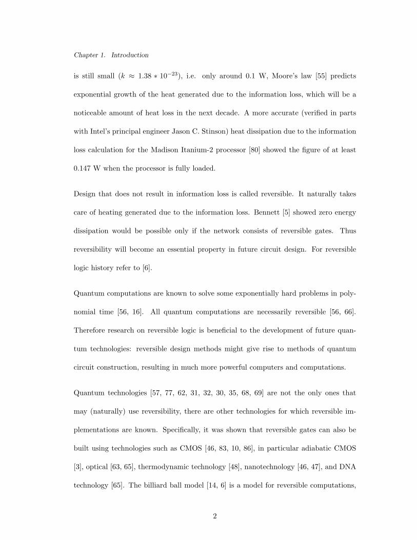
is still small (k ≈ 1.38 ∗ 10−23), i.e. only around 0.1 W, Moore’s law [55] predicts
exponential growth of the heat generated due to the information loss, which will be a
noticeable amount of heat loss in the next decade. A more accurate (verified in parts
with Intel’s principal engineer Jason C. Stinson) heat dissipation due to the information
loss calculation for the Madison Itanium-2 processor [80] showed the figure of at least
0.147 W when the processor is fully loaded.
Design that does not result in information loss is called reversible. It naturally takes
care of heating generated due to the information loss. Bennett [5] showed zero energy
dissipation would be possible only if the network consists of reversible gates. Thus
reversibility will become an essential property in future circuit design. For reversible
logic history refer to [6].
Quantum computations are known to solve some exponentially hard problems in poly-
nomial time [56, 16]. All quantum computations are necessarily reversible [56, 66].
Therefore research on reversible logic is beneficial to the development of future quan-
tum technologies: reversible design methods might give rise to methods of quantum
circuit construction, resulting in much more powerful computers and computations.
Quantum technologies [57, 77, 62, 31, 32, 30, 35, 68, 69] are not the only ones that
may (naturally) use reversibility, there are other technologies for which reversible im-
plementations are known. Specifically, it was shown that reversible gates can also be
built using technologies such as CMOS [46, 83, 10, 86], in particular adiabatic CMOS
[3], optical [63, 65], thermodynamic technology [48], nanotechnology [46, 47], and DNA
technology [65]. The billiard ball model [14, 6] is a model for reversible computations,
2
Chapter 1. Introduction
which among others, was simulated with reversible cellular arrays [38]. It happens that
reversible logic naturally appears in many applications that initially do not seem to be
connected to reversible logic at all, such as complex antenna simulations [76]. But the
essence of the simulation, a process of propagating a wave, is essentially a reversible
transformation. We do not discuss the different technologies in detail, since some of
their descriptions involve deep knowledge of physics, electronics, circuitry, quantum
mechanics, optics, thermodynamics and other physical/engineering subjects.
Most gates used in digital design are not reversible. For example the AND, OR and
EXOR gates do not perform reversible operations. Of the commonly used gates, only
the NOT gate is reversible. A set of reversible gates is needed to design reversible
circuits. Several such gates have been proposed over the past decades. Among them
are the controlled-not (CNOT) proposed by Feynman [13], Toffoli [82], and Fredkin [14]
gates. These gates have been studied in detail. However, good synthesis methods have
not emerged. Shende et al. [74, 75] suggest a synthesis method that produces a minimal
circuit with up to 3 input variables. Iwama et al. [22] describe transformation rules for
CNOT based circuits. These rules may be of use in a synthesis method. Miller [49]
uses spectral techniques to find near optimal circuits. Mishchenko and Perkowski [54]
suggest a regular structure of reversible wave cascades and show that such a structure
would require no more cascades than product terms in an ESOP (“exclusive or” sum of
products) realization of the function. In fact, one would expect that a better method
can be found. The algorithm sketched in [54] has not been implemented. A regular
symmetric structure has been proposed by Perkowski et al. [60] to realize symmetric
functions. The reversible logic design algorithms will be considered in the Literature
3
Chapter 1. Introduction
Overview chapter in detail.
Traditional design methods use, among other criteria, the number of gates as a com-
plexity measure (sometimes taken with some specific weights reflecting the area of the
gate). From the point of view of reversible logic we have one more factor which is more
important than the number of gates used, namely the number of garbage outputs. Since
reversible design methods use reversible gates, where the number of inputs is equal to
the number of outputs, the total number of outputs of such a network will be equal to
the number of inputs. The existing methods [54] use the analogy of copying information
from the input of the network, therefore introducing garbage outputs—information that
we do not need for the computation. In some cases garbage is unavoidable. For exam-
ple, a single output function of n variables will require at least n − 1 garbage outputs,
since reversibility necessitates an equal number of outputs and inputs.
The importance of minimizing garbage is illustrated with the following example. Say
we want to realize a 5 input 3 output function in a reversible method on a quantum
computer, but the design requires 7 additional garbage outputs (that is 5 constant
inputs), resulting in a 10-input 10-output reversible function. In the year 2002 the best
quantum computer has 7 qubits [1], therefore we will not be able to implement this
design. In other words, in the case of choosing between increasing the garbage and
increasing the number of gates in a reversible implementation, the preference should be
given to the design method delivering the minimum amount of garbage. In this case we
will be able to build the device, while it is impossible with the other method.
The presented work is organized as follows.
4

Chapter 1. Introduction
• In the chapter Basic Definitions and Literature Overview the classic objects
from reversible logic theory are defined. With this introductory part the reader
becomes familiar with the objectives and notations of reversible logic theory. Pre-
vious work is analyzed and summarized in this section. As an important part of
this summary, the weaknesses of previous approaches are pointed out.
• The first step in our research is the attempt to minimize the garbage that is the
major weakness in all existing methods. The chapter Reversible Cascades with
Minimal Garbage is focused on the conditions for minimal garbage, introduces
and analyzes the new model that allows synthesis with minimal garbage, suggests
possible design algorithms for both reversible and multiple output functions, dis-
cusses implementation of the algorithms and results of their testing, compares
the proposed algorithms to known ones, and analyzes the quantum cost of the
model. Finally, we compare efficiency of the new model to the efficiency of a pop-
ular model for non-reversible synthesis, EXOR PLA (“exclusive or” programmable
logic array [70]). The results of the RCMG model and synthesis using it can be
found in three of our works: [11], [45], [40] and Miller’s work [50].
• In the next chapter, Toffoli Synthesis, the conventional Toffoli gates were cho-
sen to form the set of model gates. We create a theoretical synthesis method that
initially produces acceptable size networks and show its modification, the bidirec-
tional algorithm. Since, even after the bidirectional algorithm successfully termi-
nates the circuit may still not be optimal, the following heuristic simplification
procedures are applied: output permutation, control input reduction, choosing
between realizing f and inverting the network for f−1, applying a template tool.
5
Chapter 1. Introduction
The last simplification procedure seems to be the most promising from the point
of view of the network simplification, therefore the templates are properly defined,
classified, and applied. For some small parameters the set of all templates is com-
pletely built. The algorithm and simplification procedures are implemented and
tested on benchmark functions. In addition to the commonly used benchmark
functions we also create our own benchmark functions, the functions for which
the method produces a large network and analyze why it happens. Some of the
results of this chapter can also be found in our works [51, 42] and [43].
• The Toffoli gates are not the only gates that are widely used. There are also such
gates as the Fredkin gate, Miller gate, Kerntopf gate and many more. The Fredkin
gate can be generalized and incorporated into the algorithm initially designed
for Toffoli network synthesis. In the chapter Toffoli-Fredkin Synthesis both
versions of the algorithm and all the simplification procedures from the previous
chapter are updated and applied to the new network model consisting of Toffoli and
Fredkin gates. The new family of gates differs from the Toffoli gates only, therefore
the new template classification is shown. Again, the results were implemented
and tested on benchmark functions. As part of this testing, the results of the
algorithm application are compared with the optimal Toffoli-Fredkin networks for
all 3-input 3-output reversible functions. Part of the research done in this chapter
can be found in the following of our publications [51, 12, 41].
• Most of the classical synthesis methods for the conventional logic synthesis are
asymptotically optimal. Reversible logic is a new area and it does not have an
asymptotically optimal synthesis method. In the chapter Asymptotically Opti-
6

Chapter 1. Introduction
mal Regular Synthesis we introduce a new mEXOR model and show an optimal
synthesis (in terms of the number of gates used in the resulting design) method
for it. We also show that technologically it is not expensive to create the gates
for this new model, in fact their quantum cost differs only marginally from the
quantum cost of conventional Toffoli gates. This chapter has been published as
[39].
• The chapter Dynamic Programming Algorithms as Reversible Circuits:
Symmetric Function Realization talks about synthesizing some recursive func-
tions as a network of Toffoli gates. An example of recursive functions is the set of
symmetric functions. We show how to build inexpensive quantum circuits for any
multiple output symmetric function.
• The chapter Further Research points to the directions of the further research
in the reversible logic area.
• The dissertation concludes with the chapter Summary which highlights the ac-
complishments described in this thesis.
7

Chapter 2Basic Definitions and LiteratureOverview
2.1 Boolean Algebra
We start with a brief overview of Boolean logic. There are two Boolean constants, 0 and
1. One method to describe (and, therefore, define) a Boolean function f(x1, x2, ..., xn)
of n variables is by a truth table. This construction is a table with (n + 1) columns
and 2n rows. In the rightmost column the value of the function for the input that is
placed in the first n columns is given for each row. The number of different inputs for
a function of n Boolean variables is 2n, therefore the height of this construction is 2n.
In other words, the truth table has 2n rows. Note that all the 2n Boolean patterns are
arranged in lexicographical order, and this reflects the conventional way of writing the
truth table. It can be seen that the truth table requires a lot of storage space though the
information about the order of inputs is not important, since it can be easily restored
from the information on which string of the truth table are we looking at. In order to
simplify the format, the truth vector method is used. The truth vector for a function of
n variables is the sequence of Boolean numbers of length 2n, where the k-th number of
this sequence is the value of the function on the input that is the binary representation
of number (k − 1). In the following example we see the advantage of the truth vector
8
Chapter 2. Basic Definitions and Literature Overview
method of representing a function compared with the truth table method.
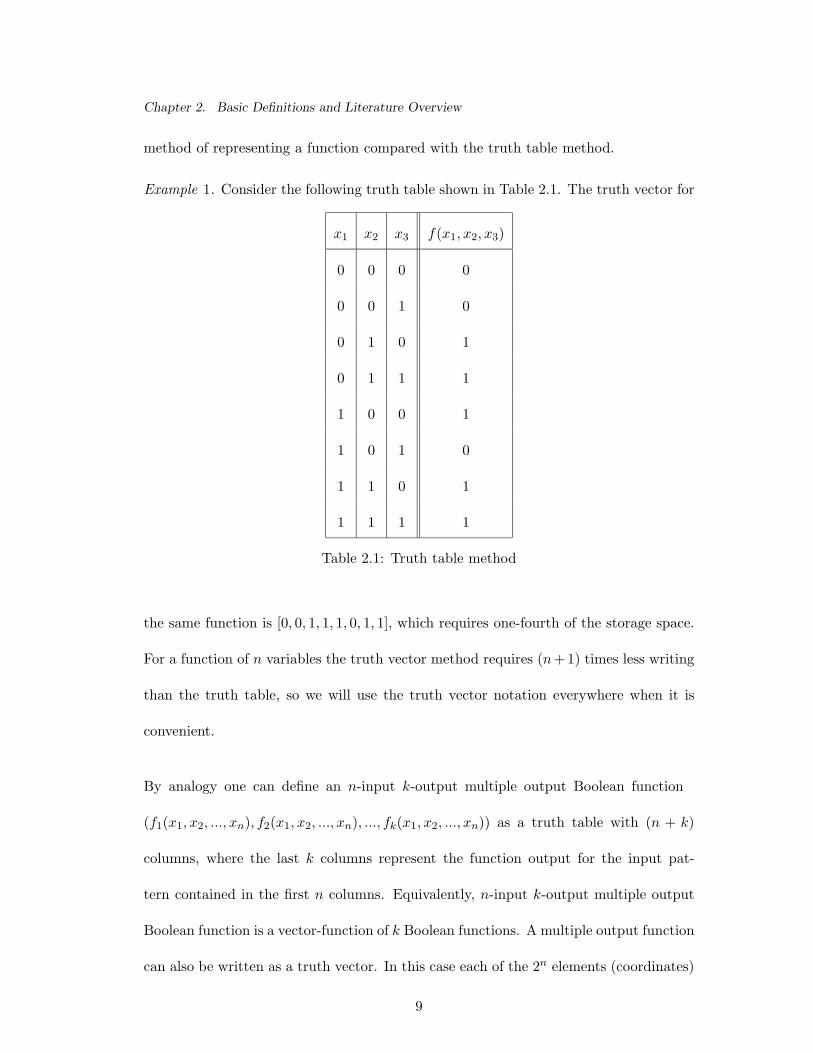
Example 1. Consider the following truth table shown in Table 2.1. The truth vector for
x1 x2 x3 f(x1, x2, x3)
0 0 0 0
0 0 1 0
0 1 0 1
0 1 1 1
1 0 0 1
1 0 1 0
1 1 0 1
1 1 1 1
Table 2.1: Truth table method
the same function is [0, 0, 1, 1, 1, 0, 1, 1], which requires one-fourth of the storage space.
For a function of n variables the truth vector method requires (n+1) times less writing
than the truth table, so we will use the truth vector notation everywhere when it is
convenient.
By analogy one can define an n-input k-output multiple output Boolean function
(f1(x1, x2, ..., xn), f2(x1, x2, ..., xn), ..., fk(x1, x2, ..., xn)) as a truth table with (n + k)
columns, where the last k columns represent the function output for the input pat-
tern contained in the first n columns. Equivalently, n-input k-output multiple output
Boolean function is a vector-function of k Boolean functions. A multiple output function
can also be written as a truth vector. In this case each of the 2n elements (coordinates)
9
Chapter 2. Basic Definitions and Literature Overview
of this vector is an integer number in the interval [0..2k − 1] which is the binary repre-
sentation of the output pattern.
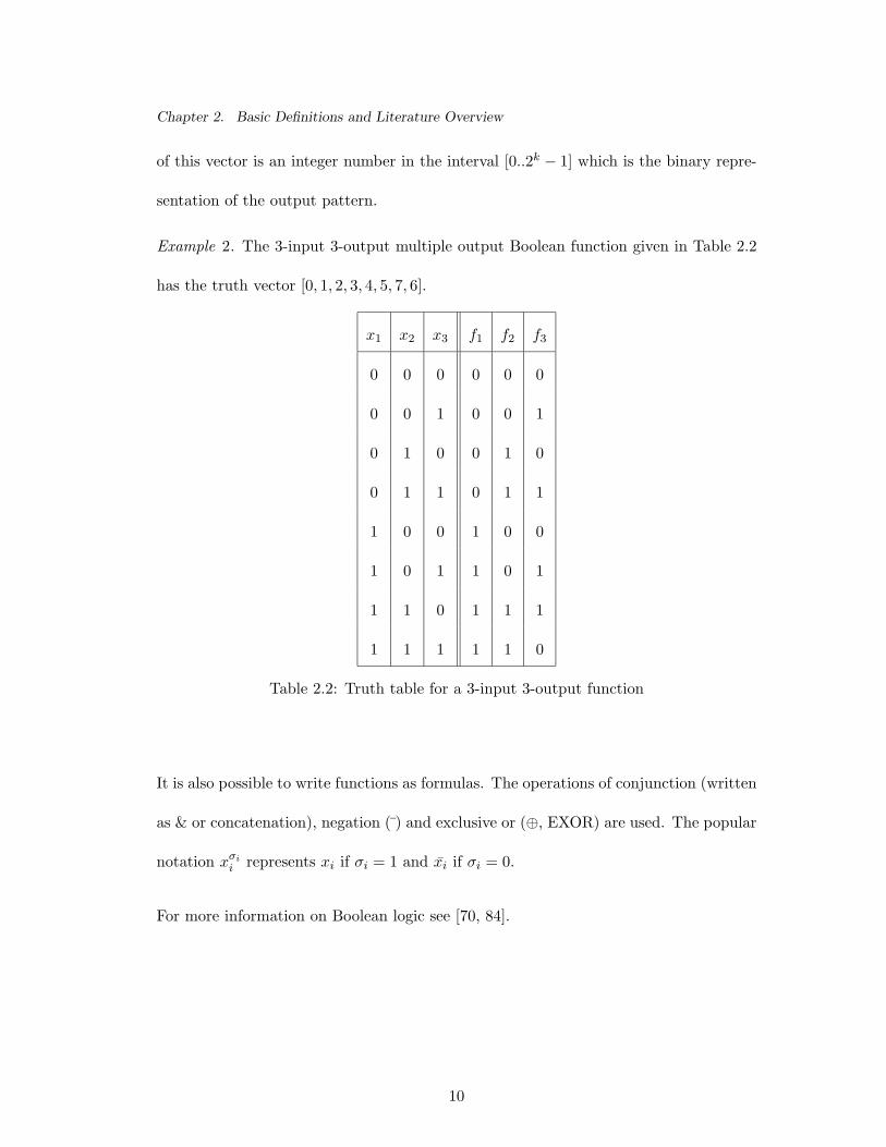
Example 2. The 3-input 3-output multiple output Boolean function given in Table 2.2
has the truth vector [0, 1, 2, 3, 4, 5, 7, 6].
x1 x2 x3 f1 f2 f3
0 0 0 0 0 0
0 0 1 0 0 1
0 1 0 0 1 0
0 1 1 0 1 1
1 0 0 1 0 0
1 0 1 1 0 1
1 1 0 1 1 1
1 1 1 1 1 0
Table 2.2: Truth table for a 3-input 3-output function
It is also possible to write functions as formulas. The operations of conjunction (written
as & or concatenation), negation ( ) and exclusive or (⊕, EXOR) are used. The popular
notation xσii represents xi if σi = 1 and xi if σi = 0.
For more information on Boolean logic see [70, 84].
10
Chapter 2. Basic Definitions and Literature Overview
2.2 Basic Definitions of the Reversible Logic
The main object in reversible logic theory is the reversible function, which is defined as
follows.
Definition 1. The multiple output Boolean function F (x1, x2, ..., xn) of n Boolean
variables is called reversible if:
1. the number of outputs is equal to the number of inputs;
2. any output pattern has a unique preimage.
In other words, reversible functions are those that perform permutations of the set of
input vectors.
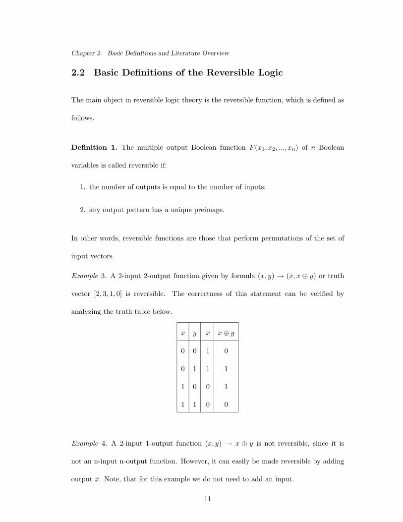
Example 3. A 2-input 2-output function given by formula (x, y) → (x, x ⊕ y) or truth
vector [2, 3, 1, 0] is reversible. The correctness of this statement can be verified by
analyzing the truth table below.
x y x x ⊕ y
0 0 1 0
0 1 1 1
1 0 0 1
1 1 0 0
Example 4. A 2-input 1-output function (x, y) → x ⊕ y is not reversible, since it is
not an n-input n-output function. However, it can easily be made reversible by adding
output x. Note, that for this example we do not need to add an input.
11
Chapter 2. Basic Definitions and Literature Overview
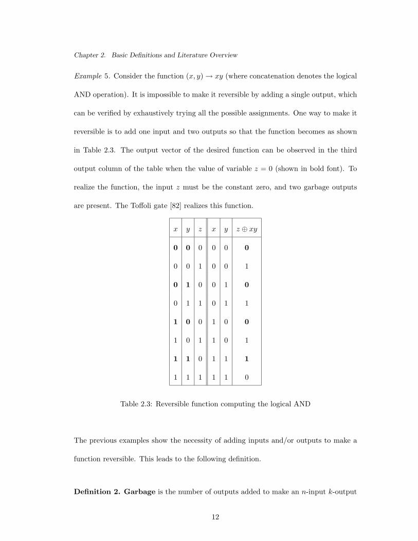
Example 5. Consider the function (x, y) → xy (where concatenation denotes the logical
AND operation). It is impossible to make it reversible by adding a single output, which
can be verified by exhaustively trying all the possible assignments. One way to make it
reversible is to add one input and two outputs so that the function becomes as shown
in Table 2.3. The output vector of the desired function can be observed in the third
output column of the table when the value of variable z = 0 (shown in bold font). To
realize the function, the input z must be the constant zero, and two garbage outputs
are present. The Toffoli gate [82] realizes this function.
x y z x y z ⊕ xy
0 0 0 0 0 0
0 0 1 0 0 1
0 1 0 0 1 0
0 1 1 0 1 1
1 0 0 1 0 0
1 0 1 1 0 1
1 1 0 1 1 1
1 1 1 1 1 0
Table 2.3: Reversible function computing the logical AND
The previous examples show the necessity of adding inputs and/or outputs to make a
function reversible. This leads to the following definition.
Definition 2. Garbage is the number of outputs added to make an n-input k-output
12
Chapter 2. Basic Definitions and Literature Overview
function ((n, k) function) reversible.
We use the words “constant inputs” to denote the preset value inputs that were added to
an (n, k) function to make it reversible. In the previous example a single constant input
was added, namely the variable z with value 0. In general, if a reversible implementation
with “constant inputs” of a function is given, the function itself can be calculated by
assigning zeros and ones to the “constant inputs”.
The following simple formula shows the relation between the number of garbage outputs
and constant inputs
input + constant input = output + garbage.
2.2.1 Network Structure
No fan-outs and no feed-back is a natural restriction for building quantum networks, and
reversible logic is usually considered with the quantum technology in mind. Thus, due to
existing technological restrictions also likely for incompletely developed technologies, the
synthesis of reversible logic is done with the conventional agreements: no feed-backs and
no fan-outs are allowed [56]. This leaves us with the cascade structure as the only model
satisfying those conditions. (A cascade is any circuit with S gates G1, G2, ... , GS where
no two gates are activated at the same time: Gi works only when Gi−1 has produced
an output. In other words, cascade defines a total order on the set of gates induced by
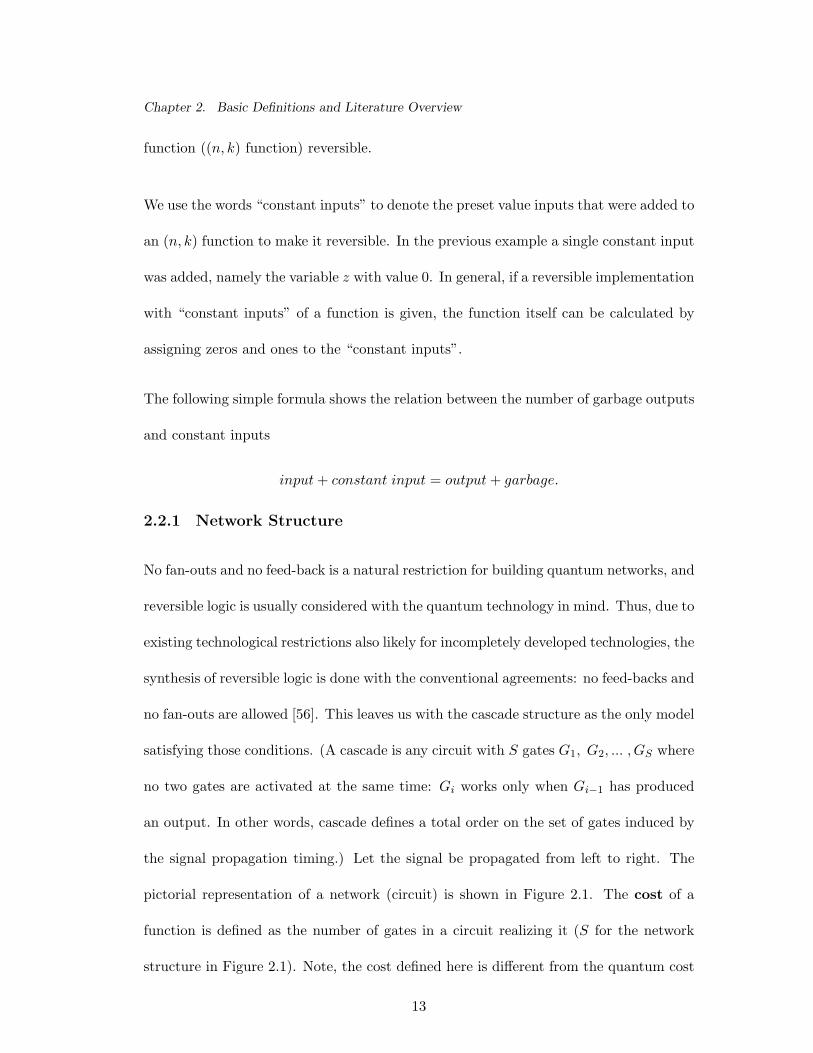
the signal propagation timing.) Let the signal be propagated from left to right. The
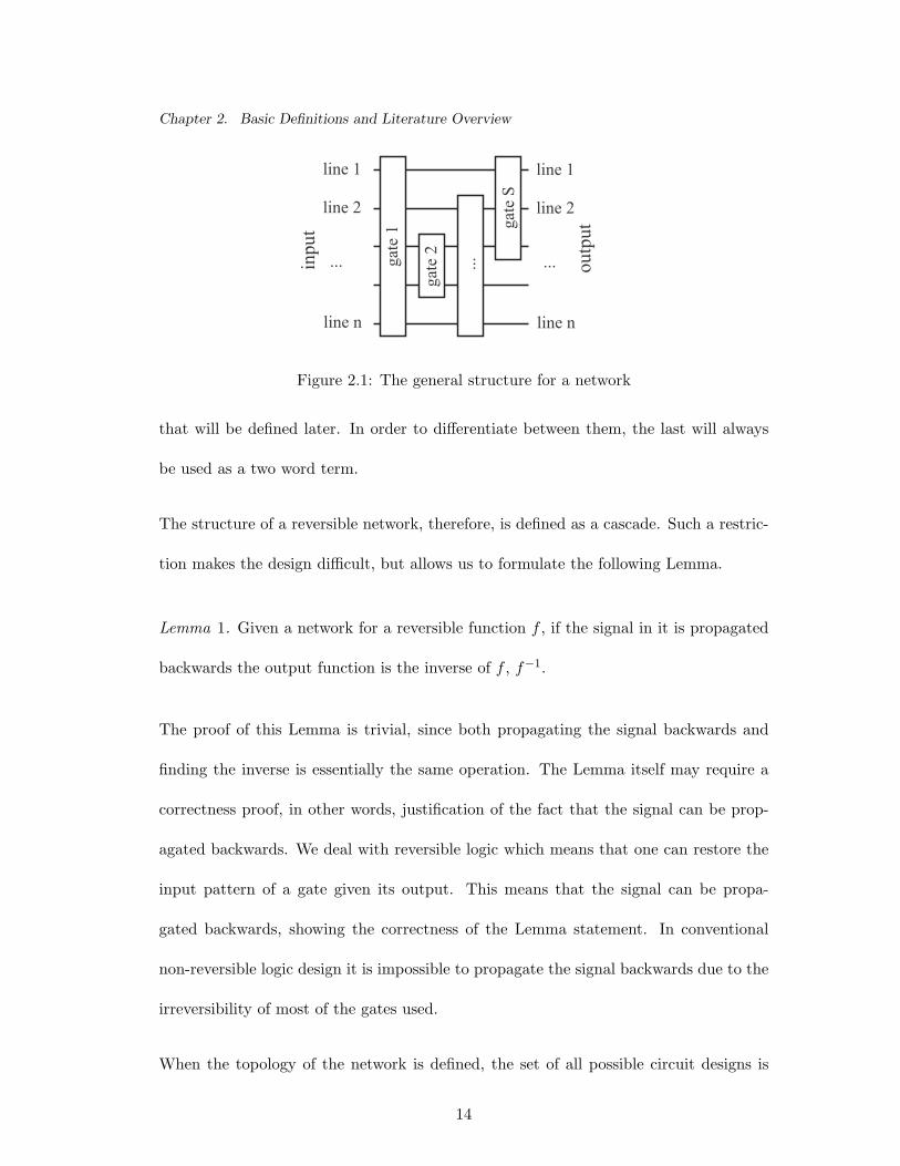
pictorial representation of a network (circuit) is shown in Figure 2.1. The cost of a
function is defined as the number of gates in a circuit realizing it (S for the network
structure in Figure 2.1). Note, the cost defined here is different from the quantum cost
13
Chapter 2. Basic Definitions and Literature Overview
inpu
t
outp
ut
gate
1
line 1
line 2
...
line n
gate
2
...
gate
S
line 1
line 2
...
line n
Figure 2.1: The general structure for a network
that will be defined later. In order to differentiate between them, the last will always
be used as a two word term.
The structure of a reversible network, therefore, is defined as a cascade. Such a restric-
tion makes the design difficult, but allows us to formulate the following Lemma.
Lemma 1. Given a network for a reversible function f , if the signal in it is propagated
backwards the output function is the inverse of f , f−1.
The proof of this Lemma is trivial, since both propagating the signal backwards and
finding the inverse is essentially the same operation. The Lemma itself may require a
correctness proof, in other words, justification of the fact that the signal can be prop-
agated backwards. We deal with reversible logic which means that one can restore the
input pattern of a gate given its output. This means that the signal can be propa-
gated backwards, showing the correctness of the Lemma statement. In conventional
non-reversible logic design it is impossible to propagate the signal backwards due to the
irreversibility of most of the gates used.
When the topology of the network is defined, the set of all possible circuit designs is
14
Chapter 2. Basic Definitions and Literature Overview
strongly restricted. The only thing that we may still vary is which transformations the
actual gates may do. The transformations themselves are strongly dependent on the
size of a gate.
Definition 3. The size of a reversible gate is a natural number which shows the number
of its inputs (outputs).
In the following subsections we introduce the gates starting from the most popular and
widely used Toffoli and Fredkin gates and ending with the more recent and less used
Picton gate, Kerntopf gate, Miller gate, Khan gate, etc.
2.2.2 The Popular Reversible Gates: Fredkin and Toffoli
In this subsection we define the popular Toffoli and Fredkin gates.
Definition 4. For the set of domain variables {x1, x2, ..., xn} the generalized Toffoli
gate has the form TOF (C; T ), where C = {xi1 , xi2 , ..., xik}, T = {xj} and C∩T = ∅. It
maps a Boolean pattern (x01, x
02, ..., x
0n) to (x0
1, x02, ..., x
0j−1, x
0j ⊕x0
i1x0
i2...x0
ik, x0
j+1, ..., x0n).
In the literature, a number of gates from the set of all generalized Toffoli gates were
considered. The most popular are: the NOT gate (TOF (xj)), a generalized Toffoli gate
which has no controls; the CNOT gate (TOF (xi; xj))[13], which is also known as the
Feynman gate, a generalized Toffoli gate with one control bit; and the original Toffoli
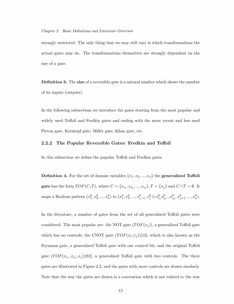
gate (TOF (xi1 , xi2 ; xj))[82], a generalized Toffoli gate with two controls. The three
gates are illustrated in Figure 2.2, and the gates with more controls are drawn similarly.
Note that the way the gates are drawn is a convention which is not related to the way
15
Chapter 2. Basic Definitions and Literature Overview
target
control
control
NOT CNOT(Feynman)
Toffoli
Figure 2.2: NOT, CNOT and Toffoli gates
the gates are implemented. Gates with more than two controls are discussed in [56, 39].
The set of generalized Toffoli gates is proven to be complete (for example, see [45]); in
other words, any reversible function can be realized as a cascade of Toffoli gates.
Definition 5. For the set of domain variables {x1, x2, ..., xn} the generalized Fredkin
gate has the form FRE(C; T ), where C = {xi1 , xi2 , ..., xik}, T = {xj , xl} and C ∩ T =
∅. It maps a Boolean pattern (x01, x
02, ..., x
0n) to (x0
1, x02, ..., x
0j−1, x
0l , x
0j+1, ..., x
0l−1, x
0j ,
x0l+1, ..., x
0n) if and only if x0
i1x0
i2...x0
ik= 1. In other words, the generalized Fredkin gate
interchanges bits xj and xl if the corresponding product of C equals 1.
Several cases of the generalized Fredkin gates can be found in the literature. A gate
with no controls, FRE(x1, x2), is usually called SWAP since it swaps the signals on
x1 and x2. For some technologies the SWAP is done for free, for others there is a cost
associated with it. For example, in CMOS there is no cost for interchanging the two
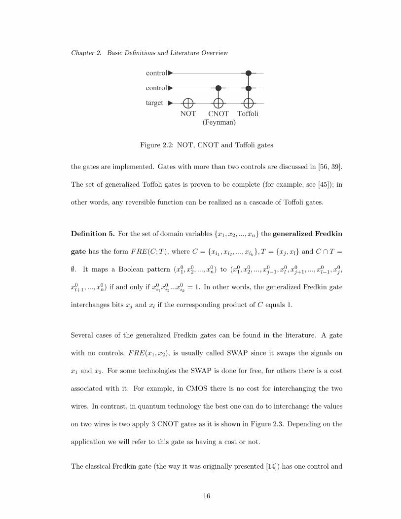
wires. In contrast, in quantum technology the best one can do to interchange the values
on two wires is two apply 3 CNOT gates as it is shown in Figure 2.3. Depending on the
application we will refer to this gate as having a cost or not.
The classical Fredkin gate (the way it was originally presented [14]) has one control and
16

Chapter 2. Basic Definitions and Literature Overview
=
Figure 2.3: SWAP gate realization in quantum technology
can be written as FRE(x1; x2, x3).
For both gates defined above set C will be called the set of controls and T will be
called the target. The number of elements in the set of controls C defines the width
of the gate.
2.2.3 Several Other Reversible Gates
There were some more reversible gates proposed in the literature.
The Kerntopf gate [23, 25] is a reversible gate of size 3 which for the inputs x, y and z
produces the output (1⊕x⊕y⊕z⊕xy, 1⊕y⊕z⊕xy⊕yz, 1⊕x⊕y⊕xz). Unfortunately,
no good implementation of this gate is known, so it is not used very often. A size k
generalization of this gate was considered in [29, 52].
The Miller gate, initially considered as a benchmark function for the spectral techniques
synthesis method in [49] has a specification given by the truth vector [0, 1, 2, 4, 3, 5, 6, 7].
The circuit of Toffoli gates of size five and quantum complexity 9 was initially proposed
as a structural representation of this gate, but later on quantum circuits of size 7 were
found [85]. This gate was recently introduced, so it is not used in the current synthesis
procedures, but seems to be useful since it affects all three bits and its quantum cost is
comparable to the quantum cost of the size 3 Toffoli gate (ratio of costs is 7 to 5) and
quantum cost of the size 3 Fredkin gate (they have the same cost). It is not clear yet
17
Chapter 2. Basic Definitions and Literature Overview
how this gate can be generalized.
The recently introduced Khan gate [27] for the input vector (x1, x2, ..., xn) produces
the output (x1, x2, ..., xn−2, fxn−1 ⊕ xn, f ¯xn−1 ⊕ xn) for an arbitrary function f =
f(x1, x2, ..., xn−2). The function f is usually the ⊕ or & of its arguments. For the
second case (operation &) the quantum complexity of such a gate was shown to be
twice as much as the complexity of the Toffoli gate with n − 2 variables. This gate
seems to be expensive and the existing synthesis procedure [28] requires a lot (growing
asymptotically faster than the minimal amount of garbage bits will be shown to be) of
garbage.
A newly shown majority-based reversible gate [85] is an odd size reversible gate, such
that at least one output is a majority Boolean function of its inputs. A majority Boolean
function is such a function that returns one if and only if more than half of its inputs
are ones. This gate seems complex in the classical Boolean circuit realization, and its
realizations in a reversible technology are not known yet. The Miller gate is a case of a
majority-based reversible gate.
The Picton gate [64] is a multi-valued logic generalization of a Fredkin gate. It is
not useful at this point since no multiple-valued reversible logic synthesis methods are
designed yet. No implementation of the Picton gate is known yet.
Among other existing gates are the Perkowski gates [29, 62], Margolus gates [24], and De-
Vos gates [25]. We do not introduce these gates here, since to the best of our knowledge
they were not yet used. However, one of the gates Perkowski mentions in [62] seems to be
a useful one, since for the input (x1, x2, x3) it produces the output (x1, x1⊕x2, x3⊕x1x2)
18

Chapter 2. Basic Definitions and Literature Overview
when a quantum circuit with cost only 4 (which is less than the cost of a Toffoli gate)
was found. Perkowski also states [62] that this implementation was known to Peres [57].
2.3 Overview of Reversible Logic Synthesis Methods
Such a variety of different reversible gates results in a variety of different approaches
to reversible logic synthesis. Fortunately, the basic analysis of different techniques of
reversible logic synthesis was successfully done in one of Perkowski’s work [85]. Here,
we use and expand this approach to the classification of reversible synthesis methods.
1. Composition methods [54, 59, 45, 11, 51, 12]. The idea is to compose a reversible
block using small and well known reversible gates. The reversible block should
be easy to use. Then, a modification of a conventional logic synthesis procedure
is applied to synthesize a network. The resulting network will be reversible as a
network essentially consisting of reversible gates.
2. Decomposition methods [59, 45]. Decomposition methods can be characterized as
a top-down reduction of the function from its outputs to its inputs. During the
design procedure a function is supposed to be decomposed into a combination of
several specific functions each of which is realized as a separate reversible network.
An example of a decomposition method can be found in [45] where synthesis
appears to be a reduction of the output to the form of the input.
The decomposition and composition methods can be multilevel. Observe that
the composition and decomposition methods form a very general and powerful
tool of logic synthesis. In fact, most of the algorithms can be classified as either
composition or decomposition. Using Lemma 1, one can notice the duality of the
19
Chapter 2. Basic Definitions and Literature Overview
composition and decomposition methods; a composition design procedure for a
reversible function f is a decomposition procedure for f−1.
3. Factorization methods [28]. Factorization is another powerful logic design tool.
Its idea is in choosing a Boolean operation, for instance, ? (often multiplication
or EXOR) for a function f and finding two functions f1 and f2 such that:
• f = f1 ? f2;
• for the synthesis cost metrics the cost of f is smaller than the sum of costs
of f1 and f2 plus a weight associated with the ? operation.
In general, the ? operation does not have to be a binary operation, but may be an
arbitrary multiple output function of several arguments. To our knowledge, the
factorization tool was first applied to reversible logic design in [28].
4. EXOR logic based methods [22, 59, 74, 75, 51, 42]. The Toffoli gate uses the
EXOR operation in its definition since when it is used the gate can be described
as a simplest formula. Usage of the properties of the EXOR operation such as:
• a ⊕ b = b ⊕ a;
• a ⊕ 0 = a;
• a ⊕ 1 = a;
• a ⊕ a = 0;
allows heuristic synthesis [59] and simplification of the already created networks
[22, 74, 75, 51, 42]. For example, Iwama et al. [22] describe transformation rules
for CNOT based circuits. The input of their method is a reversible circuit of
20

Chapter 2. Basic Definitions and Literature Overview
Toffoli elements, and the output is a canonical form reversible circuit of the Tof-
foli elements. This canonical form is a straightforward reversible implementation
of PPRM (Positive Polarity Reed-Muller expansion), also known as a Zhegalkin
polynomial. Iwama et al. [22] prove that any circuit can be brought to a canonical
form by certain (reversible) operations, thus a canonical form can be transformed
to a minimal circuit. Unfortunately, they do not provide any method of simpli-
fying a circuit by the set of transformations they have, so the paper is more for
theoretical interest. In general, the EXOR operation is very hard to analyze (in
fact, the best Boolean EXOR polynomials were found only for functions of at most
6 variables [15]), therefore only heuristic approaches currently work.
5. Genetic algorithms [36, 62]. The general idea behind genetic algorithms is emu-
lation of the evolution process. First, several possible solutions or initial guesses
are coded by strings and the fitness function is defined. The fitness function rep-
resents the probability of “survival” of a string. The strings which are close to
the desired solution usually have a high fitness value. At the first part of the life
cycle, a crossing over operation is used to create the new strings out of the set
of strings available. At the second stage, mutation operations are applied. The
cycle finishes with the application of the fitness operation, which takes away some
of the strings. The new cycle begins. After several applications of this cycle (sev-
eral generations) the strings with the best fitness value are read. These genetic
algorithms have a lot of formulations and their actual implementations may vary.
Their main weakness is their extremely bad scaleability.
6. Search, backtracking, simulated annealing, etc. [29, 54, 59, 11, 12]. Backtracking
21

Chapter 2. Basic Definitions and Literature Overview
or look-ahead techniques are widely used in heuristic approximations of a desired
object. Their fundamental characteristic is in considering several steps ahead and
making a decision on a small change based on the information that this change
may result in. This technique is very expensive to use, since each vertex of the
decision tree branches and the size of the search space grows exponentially with
only a linear increase in the depth of the search. Simulated annealing is an idea
that comes from the cooling of metals. If the liquid metal is cooled very fast, the
structure of its lattice will not be regular and it will be easy to break such a metal.
If during the cooling process the metal is cooled and then slightly warmed, then
cooled and again warmed a little, and so on, the final molecular lattice of the metal
detail will be more regular, thus resulting in higher durability and robustness. The
same idea may work with circuit design: take a circuit and start expanding and
reducing it without changing its output functionality. After a certain number of
such operations, a more compact circuit may be found.
7. Group-theoretic methods including use of algebraic software such as GAP [73,
81, 85]. The set of all reversible functions forms a non-Abelian group (denoted
Sn) with respect to the composition operation. The group of all permutations of
n elements Sn is very well investigated. The first nice property of the group is
that if a reversible function f can be written as a composition of several other
permutations f = f1 ◦f2 ◦ ...◦fk, its circuit is a cascade of circuits for f1, f2, ..., fk.
So, circuit design is equivalent to the problem of finding a simple composition of
easy to build permutations. Small size generating sets can be found for the group
of all permutations, therefore producing a small and complete set of gates. In other
22
Chapter 2. Basic Definitions and Literature Overview
words, searching for new gates is possible with a group theoretic approach. In our
opinion, group theoretical approaches have not been investigated at a proper level
yet. One of the unavoidable weaknesses of this approach is its need for a reversible
specification.
8. Synthesis of regular structures such as nets [60, 61], lattices [2], and PLAs [65].
The idea behind these methods is creating conventional logic design objects out of
reversible components and then applying the known techniques of logic synthesis
to create reversible specifications. Such methods usually have a very high amount
of garbage which makes it impossible to use such designs in technologies with
the high cost of garbage, such as quantum technology. Also, one would expect
that reducing reversible synthesis to conventional non-reversible synthesis cannot
produce good results due to the different nature of the objects.
9. Spectral techniques by Miller [49, 50]. The spectrum [21] of a Boolean function is
its correlation with the vector of length 2n of all linear monotonically increasing
functions. In both of his works, Miller applied a composition approach with the
decision of choosing the gate based on the spectral complexity. If addition of a
gate to a cascade decreases the spectral complexity, then it is added. In practice,
such a gate has always existed. The method produces good results for small size
reversible functions, but it has its weaknesses: it scales badly, and requires a
reversible specification.
10. Exhaustive search [58, 74, 75]. Minimal circuits for reversible Boolean functions
of one variable are not interesting. There are only two reversible functions of one
23
Chapter 2. Basic Definitions and Literature Overview
variable: identity and NOT, which require 0 and 1 gates respectively. A search
of minimal circuits of 2 variable reversible functions was done by Perkowski in
his lecture notes [58] on reversible logic synthesis. Shende et al. [74, 75] search
exhaustively for minimal circuits of all reversible functions of 3 variables. It can be
shown that the number of reversible functions of n variables is 2n!, which for n = 4
becomes 24! = 16! = 20922789888000 ≈ 2 ∗ 1013. Even if each reversible function
requires one bit of storage, this results in 2345 Terabytes of storage, which does
not seem to be feasible with current technology. Thus, exhaustive search cannot
go any further at the present time.
11. Non-regular a-priori synthesis procedures, when the synthesis of the small circuits
is done mostly by hand [8].
2.4 Related Work
A few of the early presented works are similar to reversible logic. For example, inter-
esting results were obtained by Sasao et al. in years 1976-1979 [33, 72]. The authors
considered synthesis with multiple-output logic gates where the numbers of ones in the
input and the output are equal. These works are not quite in the area of reversible logic,
although reversibility implies equality of the number of ones in the input and output
domain. The authors considered equality of the ones for any input-output correspon-
dence (which, in some sense, can be treated as a power set of the set of reversible logic
functions).
In the year 2003 Sasao [71] has published an algorithm of n-input Boolean one output
multiple-valued function synthesis by reversible cascades. However, his mathematical
24

Chapter 2. Basic Definitions and Literature Overview
structure does not have a straightforward technological intuition, therefore these results
are likely to stay theoretical.
In the 1960s, Lupanov [37] considered general synthesis theory with k-input s-output
gates and with no fan-out restrictions. Thus, the structure of a network is a cascade,
which is absolutely the same as in the reversible case. The difference is in the manda-
tory reversibility of a single building block for the reversible case. Such a restriction
is not present in Lupanov’s work. The mentioned paper is very general and further
investigation is needed in order to be able to apply the published results to reversible
logic and its synthesis. Also, a high amount of garbage is expected to be added, which
makes it unlikely that the results will be applicable in a technology.
25

Chapter 3Reversible Cascades with MinimalGarbage
There are many ways of making a multiple output Boolean function reversible, each
requiring a different number of garbage outputs to be created. We start by analyzing the
conditions that affect the number of garbage outputs. Minimization of garbage outputs
may be even more important for some technologies than minimization of the number
of gates. For example, in NMR (Nuclear Magnetic Resonance) quantum technology
the maximum number of bits that can be used simultaneously for a computation is
limited by 7 [1]. In some other technologies (Trapped Ion, Neutral Atom, Solid State,
Superconducting, e-Helium, Spectral Hole Burning) introducing a garbage bit may be
possible without any restriction on the number of bits added, however it is not easy do
to [20]. In optic quantum technology garbage does not seem to cause a large problem
[20].
We further analyze the garbage amount for existing synthesis methods. A conclusion
of this analysis can be summarized in a few words: the garbage is excessive, therefore a
different approach/model should be created.
For this new model, first, and very important requirement, is few garbage outputs. What
26
Chapter 3. Reversible Cascades with Minimal Garbage
we build, in fact, has theoretically minimal number of garbage bits. Second, the model
gates should have a reasonable cost if implemented in at least one of the technologies
that support reversible logic implementations. In this thesis, a paper by Barenco et
al. [4] is used as a basis for quantum cost calculation. Unfortunately, Barenco et al.
consider only an approximation for a quantum cost calculation, where any one-qubit
and controlled-V gates [56] have a unit cost. Real quantum cost for a real technology is
different, but research laboratories who possess tools for real quantum cost calculation
do not want to share the information (partially because their quantum cost calculation
are designed specifically for their unique equipment). However, paper by Barenco et al.
gives reasonable approximation of the actual technological cost of the gates.
Finally, the results of the actual synthesis (that is, number of gates in a cascade) should
not be large in comparison to the other synthesis method results. If such a model will
be created, it may be very important for evolving further reversible logic theory and
bringing its theoretical results to the actual technology (NMR-oriented).
In our new model we consider generalization of the n-bit Toffoli gate, where input
variables can be optionally negated. Negations are technologically easy operations, and
the n-bit Toffoli gates have reasonably low (linear) cost. Thus, the model gates are
not be expensive and the second requirement on the model is satisfied. When the
set of model gates is set and geometry of the circuit is chosen (cascades in our case),
there comes the problem of synthesis: given a multiple-output Boolean function, find
a cascade of the gates from the given model which realizes it. This problem is solved
by the following procedure. First, find the minimal garbage required by the function
27

Chapter 3. Reversible Cascades with Minimal Garbage
to be able to decomposed into a set of reversible cascades (this number is independent
of the synthesis model). Then, the ways of building a circuit split into theoretical and
practical. In theoretical, a minimal reversible specification of the given multiple output
function is found and then, a reversible function is synthesized by a procedure which
always terminates with a valid circuit. This guarantees minimality of garbage, but
the number of cascades in the resulting circuit may be large. Therefore, a practical
approach was designed. It works as follows. When the amount of garbage for minimal
reversible specification is found, the corresponding number of variables is added to the
multiple output function without specifying them (“don’t cares”). Function then is
synthesized heuristically based on the idea of decreasing Hamming distance by choosing
a gate which does it best from the set of all model gates. Such approach guarantees
minimality of garbage and is capable of producing small circuits. Theoretically, this
practical approach may never create a valid circuit (keep working forever). However, it
did converge for all the examples that we tried.
3.1 Minimal Garbage
Before we analyze the garbage in other models, we need to show a formula to calculate
the minimum amount of garbage.
Theorem 1. For an (n, k) function the minimum amount of garbage required to make it
reversible is dlog(M)e, where M is the maximum of number of times an output pattern
is repeated in the truth table.
Proof. The output of a reversible function is a permutation of its input. Therefore,
the obstacle in having a multiple output function being reversible is that some output
28
Chapter 3. Reversible Cascades with Minimal Garbage
pattern appears more than once. In order to separate these outputs we have to introduce
new inputs to assign additional bits to the output vector. If an output (o1, o2, ..., ok)
has the largest occurrence in the output vector and it appears M times, then in order
to separate different occurrences of it we need to introduce dlog(M)e new output bits.
dlog(M)e new bits will be capable of creating 2dlog(M)e ≥ M new patterns. And, since
the output (o1, o2, ..., ok) had the largest occurrence among all other outputs, all other
outputs can be easily separated from one another by means of dlog(M)e bits. ¥
3.1.1 Analysis of Garbage in Existing Methods
In this subsection we analyze garbage in proposed designs. Several of the proposed
design methods (for example [29, 74, 75], and [49]) start with a reversible function. The
garbage is introduced during a preprocessing phase, during which the function is made
reversible. Note that there are many ways in which the value of the garbage outputs can
be set. Different settings of these variables will lead to results with varying complexity.
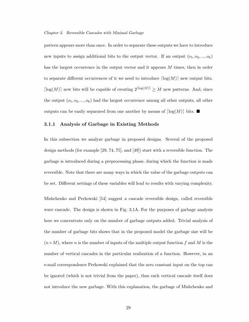
Mishchenko and Perkowski [54] suggest a cascade reversible design, called reversible
wave cascade. The design is shown in Fig. 3.1A. For the purposes of garbage analysis
here we concentrate only on the number of garbage outputs added. Trivial analysis of
the number of garbage bits shows that in the proposed model the garbage size will be
(n+M), where n is the number of inputs of the multiple output function f and M is the
number of vertical cascades in the particular realization of a function. However, in an
e-mail correspondence Perkowski explained that the zero constant input on the top can
be ignored (which is not trivial from the paper), thus each vertical cascade itself does
not introduce the new garbage. With this explanation, the garbage of Mishchenko and
29
Chapter 3. Reversible Cascades with Minimal Garbage
0
...
0
...
0
...
...
...
...
...
1
x
x
x
x1
2
3
n
F
x xx
x1
2 3 n
1
1 1 1
1
1
...
...
... ...
f f f1 2 k
0 0 0
A. Reversible wave cascades B. RPGA
Figure 3.1: Reversible design methods
Perkowski [54] method becomes n, the number of inputs of the function to be realized.
In Table 3.1 this (updated) garbage calculation is shown in brackets.
Perkowski et al. [60] suggest a regular structure for a symmetric (n, k) function reversible
design, called RPGA (Fig. 3.1B.). The synthesis for a symmetric function, as it is easy
to see from the structure Fig. 3.1B, will require garbage equal to the sum of the number
of inputs and the number of gates used (additional wires are reserved for the outputs),
which gives
n +n(n − 1)
2=
n(n + 1)2
.
Khan and Perkowski [28, 27] propose a method which has a similar structure to the one
described in [54]. The synthesis and garbage results for these methods are essentially
the same, although later work has, on average, worse results both in the number of gates
and the amount of garbage.
We calculated the number of garbage bits in the proposed model for some benchmark
30

Chapter 3. Reversible Cascades with Minimal Garbage
functions. The following table summarizes the result for the methods suggested in
[54, 60, 28] on some benchmark functions used in [54]. The first column shows the
name in out RWCG RPGAG KPG max out occur min garbage
5xp1 7 10 38(7) > 28 53 1 0
9sym 9 1 60(9) 45 60 420 9
b12 15 9 43(15) > 120 41 6944 13
clip 9 5 72(9) > 45 N/A 37 6
in7 26 10 61(26) > 351 N/A 11651840 24
rd53 5 3 19(5) 15 19 10 4
rd73 7 3 43(7) 28 47 35 6
rd84 8 4 66(8) 36 68 70 7
sao2 10 4 38(10) > 55 52 513 10
t481 16 1 29(16) > 136 28 42016 16
vg2 25 8 209(25) > 325 217 12713984 24
Table 3.1: Experimental results
name of the function, the second and third are the number of input and output bits
respectively. The fourth column is the wave cascade method garbage amount. The fifth
column is occupied by the number of garbage bits for the RPGA method given by the
formula described above. Since every non-symmetric function can be made symmetric
by adding new outputs, the procedure of making the function reversible can be done
prior to the usage of the algorithm as Perkowski et al. [60] suggest. In general, such
a procedure requires many additional inputs, each resulting in a high garbage price for
31
Chapter 3. Reversible Cascades with Minimal Garbage
their introduction. In cases where the function is not symmetric we use the sign “>”
to represent that the actual garbage amount is higher. Numbers in the sixth column
represent the garbage cost of synthesizing the Khan family gates. The seventh column
shows the maximal output occurrence, the logarithm of which added to the function
input size forms the last, eighth column, which shows the minimal garbage to be added
to make the corresponding function reversible.
We conclude this section with the observation that all three regular methods analyzed
have garbage that is far from the theoretical minimum. In the next section we introduce
a new regular structure with better garbage characteristics; in fact, the amount of
garbage is theoretically minimal.
3.2 A New Structure: Reversible Cascades with MinimalGarbage
3.2.1 Definition of the Model
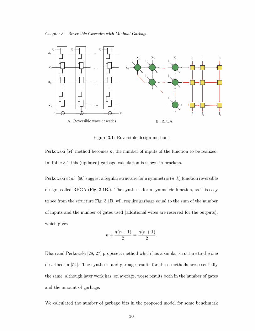
We consider the set of model gates which is a generalization of the generalized Tof-
foli gate. We use the same pictorial representation, and use (n, n)-gates where each
horizontal line is one of the following 4 types (Fig. 3.2):
xiType 1.
xiType 2.
xiType 3.
xiType 4.
Figure 3.2: Horizontal line types.
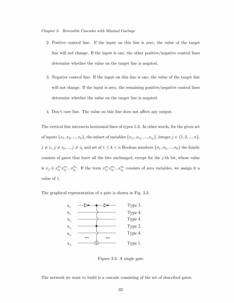
1. Target line. Each gate should have only one target line appearing at some position
j.
32
Chapter 3. Reversible Cascades with Minimal Garbage
2. Positive control line. If the input on this line is zero, the value of the target
line will not change. If the input is one, the other positive/negative control lines
determine whether the value on the target line is negated.
3. Negative control line. If the input on this line is one, the value of the target line
will not change. If the input is zero, the remaining positive/negative control lines
determine whether the value on the target line is negated.
4. Don’t care line. The value on this line does not affect any output.
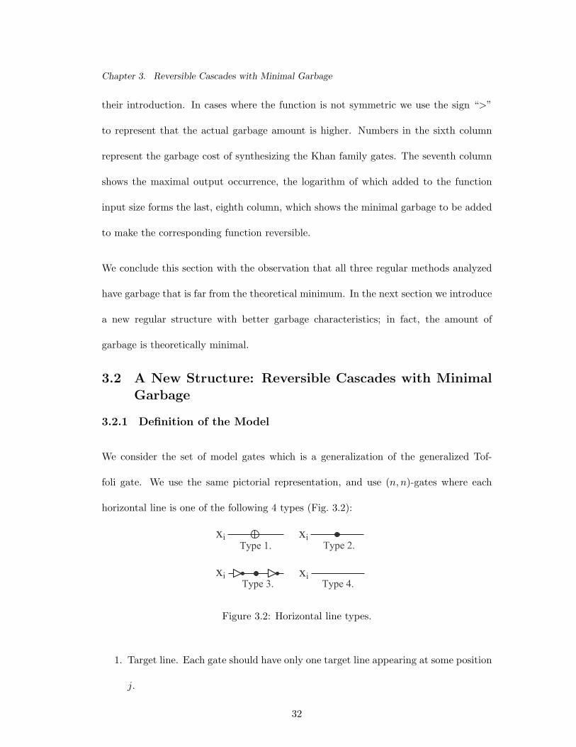
The vertical line intersects horizontal lines of types 1-3. In other words, for the given set
of inputs {x1, x2, ..., xn}, the subset of variables {xi1 , xi2 , ..., xik}, integer j ∈ {1, 2, ..., n},
j 6= i1, j 6= i2, ..., j 6= ik and set of 1 ≤ k < n Boolean numbers {σ1, σ2, ..., σk} the family
consists of gates that leave all the bits unchanged, except for the j-th bit, whose value
is xj ⊕ xσ1i1
xσ2i2
...xσkik
. If the term xσ1i1
xσ2i2
...xσkik
consists of zero variables, we assign it a
value of 1.
The graphical representation of a gate is shown in Fig. 3.3.
... ...
xxxxx
xi
i
i1
4
i
i
i
2
3
5
Type 4.
n
Type 4.Type 2.
Type 3.
Type 4.
Type 1.
Figure 3.3: A single gate
The network we want to build is a cascade consisting of the set of described gates.
33
Chapter 3. Reversible Cascades with Minimal Garbage
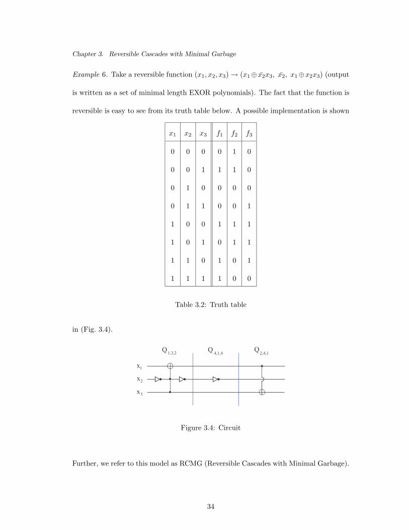
Example 6. Take a reversible function (x1, x2, x3) → (x1⊕ x2x3, x2, x1⊕x2x3) (output
is written as a set of minimal length EXOR polynomials). The fact that the function is
reversible is easy to see from its truth table below. A possible implementation is shown
x1 x2 x3 f1 f2 f3
0 0 0 0 1 0
0 0 1 1 1 0
0 1 0 0 0 0
0 1 1 0 0 1
1 0 0 1 1 1
1 0 1 0 1 1
1 1 0 1 0 1
1 1 1 1 0 0
Table 3.2: Truth table
in (Fig. 3.4).
...
x
x
x
1
2
3
Q QQ 4,1,4 2,4,11,3,2
Figure 3.4: Circuit
Further, we refer to this model as RCMG (Reversible Cascades with Minimal Garbage).
34
Chapter 3. Reversible Cascades with Minimal Garbage
3.2.2 Quantum Cost Analysis
Quantum technology is one of several technologies that uses reversible gates and com-
putations. So, it is interesting to analyze the quantum cost of the introduced model to
see whether and how it differs from the costs of the gates used by other models.
Quantum transformations are necessarily reversible, this follows from the only condition
used to determine whether a transformation can be accomplished: it must be a unitary
operator on the set of quantum state amplitudes [56]. This condition does not mention
how difficult it is to realize a given unitary transformation; it only states the theoretical
possibility.
In conjunction with reversible logic synthesis, the following transformations can be
realized as one gate with unit cost:
• NOT gate (also known as quantum X gate). For Boolean entities it acts as the
conventional NOT gate.
• CNOT gate, which acts as TOF (x1; x2). In other words, in the Boolean case it
flips x2 iff x1 = 1.
The set of gates NOT, CNOT is not complete since they only realize linear functions.
Thus, in order to make the set complete (as a set of Boolean functions), the Toffoli
gate [82], TOF (x1, x2; x3) was added. Unfortunately, this gate cannot be realized as a
single elementary quantum operation. Quantum realization of a minimal cost of 5 was
found, and it seems likely that this is the minimum. The more controls a generalized
Toffoli gate has, the larger its cost in terms of the number of elementary quantum
transformations required.
35
Chapter 3. Reversible Cascades with Minimal Garbage
The problem of building quantum blocks to realize Toffoli gates was investigated by
many authors. For a comparison of quantum costs of Toffoli and RCMG model gates
we will use results of [4]. For other implementations the costs can easily be recalculated.
Definition 6. The quantum cost of a gate G, |G| is the number of elementary quantum
operations required to realize the function given by G.
No particular realization of a gate (for most of the gates) was proven to be optimal, so
the numeric value of the quantum cost may change as soon as better gate realizations
are proposed.
To analyze the quantum cost of an RCMG model gate, we should start with its simpli-
fication, and then compare its cost to the cost of a generalized Toffoli gate. Note that
an RCMG model gate can be considered as a generalized Toffoli gate and a set of NOT
operations. First, we should try to minimize the number of NOTs in the circuit.
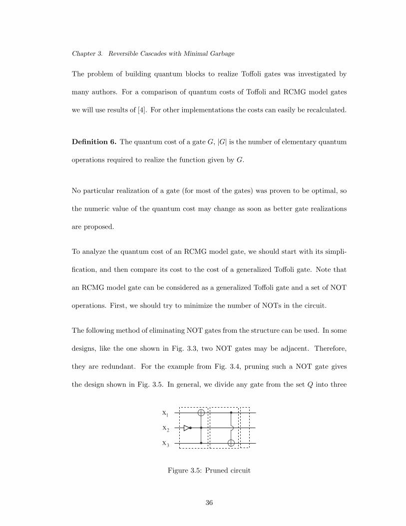
The following method of eliminating NOT gates from the structure can be used. In some
designs, like the one shown in Fig. 3.3, two NOT gates may be adjacent. Therefore,
they are redundant. For the example from Fig. 3.4, pruning such a NOT gate gives
the design shown in Fig. 3.5. In general, we divide any gate from the set Q into three
...
x
x
x
1
2
3
Figure 3.5: Pruned circuit
36
Chapter 3. Reversible Cascades with Minimal Garbage
logical parts:
• First NOT array: the set of all NOT gates before the vertical line.
• AND-EXOR array (generalized Toffoli gate): the set of all AND and EXOR gates
on the vertical line.
• Last NOT array: the set of all remaining NOT gates.
The general rule for pruning NOT gates is as follows:
1. Define TEMP array as an array of NOT gates of length n, such that there is at
most one NOT gate at each place. Initially no NOT gate is present in the TEMP
array.
2. Starting from the beginning of a particular network, keep NOTs from the first
NOT array of a first Q1 ∈ Q gate together with the next AND-EXOR array and
call this structure a block. The last NOT array of gate Q1 is called TEMP. If Q1
was one of x1, x2, ..., xn, add it to TEMP.
3. Take the next gate Q2 ∈ Q from the network. If Q2 6∈ {x1, x2, ..., xn} update the
TEMP array by computing its exclusive or with the first NOT array of Q2 that
is, keep the modulo-2 sum of number of NOTs at each wire. If the NOT gate
from the TEMP array meets a target line or a “don’t care” line, it can be passed
through the gate, so delete these occurrences from the TEMP array and add them
to the output array of the Q2 gate. Unite the TEMP array with the AND-EXOR
array (create a new block), let Q1 := Q2 and go to step 2. If the Q2 gate was
one of gates x1, x2, ..., xn, update TEMP array by computing the “exclusive or”
of TEMP with Q2, let Q1 := Q2 and go to step 2.
37
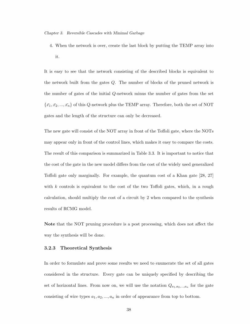
Chapter 3. Reversible Cascades with Minimal Garbage
4. When the network is over, create the last block by putting the TEMP array into
it.
It is easy to see that the network consisting of the described blocks is equivalent to
the network built from the gates Q. The number of blocks of the pruned network is
the number of gates of the initial Q-network minus the number of gates from the set
{x1, x2, ..., xn} of this Q-network plus the TEMP array. Therefore, both the set of NOT
gates and the length of the structure can only be decreased.
The new gate will consist of the NOT array in front of the Toffoli gate, where the NOTs
may appear only in front of the control lines, which makes it easy to compare the costs.
The result of this comparison is summarized in Table 3.3. It is important to notice that
the cost of the gate in the new model differs from the cost of the widely used generalized
Toffoli gate only marginally. For example, the quantum cost of a Khan gate [28, 27]
with k controls is equivalent to the cost of the two Toffoli gates, which, in a rough
calculation, should multiply the cost of a circuit by 2 when compared to the synthesis
results of RCMG model.
Note that the NOT pruning procedure is a post processing, which does not affect the
way the synthesis will be done.
3.2.3 Theoretical Synthesis
In order to formulate and prove some results we need to enumerate the set of all gates
considered in the structure. Every gate can be uniquely specified by describing the
set of horizontal lines. From now on, we will use the notation Qa1,a2,...,an for the gate
consisting of wire types a1, a2, ..., an in order of appearance from top to bottom.
38
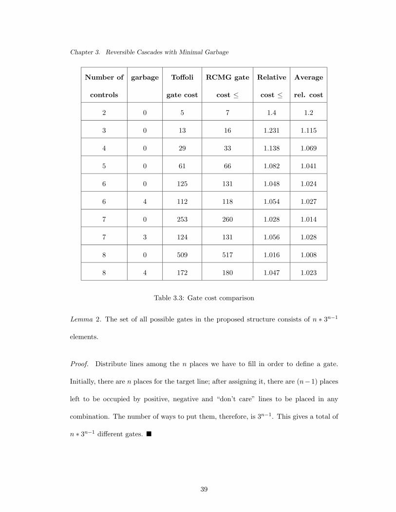
Chapter 3. Reversible Cascades with Minimal Garbage
Number of garbage Toffoli RCMG gate Relative Average
controls gate cost cost ≤ cost ≤ rel. cost
2 0 5 7 1.4 1.2
3 0 13 16 1.231 1.115
4 0 29 33 1.138 1.069
5 0 61 66 1.082 1.041
6 0 125 131 1.048 1.024
6 4 112 118 1.054 1.027
7 0 253 260 1.028 1.014
7 3 124 131 1.056 1.028
8 0 509 517 1.016 1.008
8 4 172 180 1.047 1.023
Table 3.3: Gate cost comparison
Lemma 2. The set of all possible gates in the proposed structure consists of n ∗ 3n−1
elements.
Proof. Distribute lines among the n places we have to fill in order to define a gate.
Initially, there are n places for the target line; after assigning it, there are (n−1) places
left to be occupied by positive, negative and “don’t care” lines to be placed in any
combination. The number of ways to put them, therefore, is 3n−1. This gives a total of
n ∗ 3n−1 different gates. ¥
39
Chapter 3. Reversible Cascades with Minimal Garbage
Theorem 2. (lower bound) There exists a reversible function that requires at least
2n
ln 3 + o(2n) gates.
Proof. The number of all reversible functions of n variables is 2n! (as the number of
permutations of 2n elements). The number of different gates is n3n−1. Assuming that
taking some of the gates and building networks with different orders produces different
reversible functions (which is not always true, since, for instance, the gate Q1,4,4,...,4, or
x1 placed two times at a row does nothing), we get a complexity for the hardest function
of logn3n−1(2n!). This means that there exists a reversible function which can be realized
with a complexity not less than logn3n−1(2n!). Using the formula ln(k!) = k ln k−k+o(k)
(which can be derived from Stirling’s formula) for k = 2n write:
logn3n−1(2n!) =ln(2n!)
ln(n3n−1)=
2n ln 2n − 2n + o(2n)ln(3n−1) + ln(n)
=n2n − 2n + o(2n)
(n − 1) ln 3 + ln(n)
=(n − 1)2n + o(2n)(n − 1) ln 3 + ln(n)
=2n + o(2n/n)
ln 3 +ln(n)n − 1
=2n
ln 3+ o(2n).
¥
Theorem 3. (upper bound) Every reversible function can be realized with no more
than n2n gates.
Proof. We use an idea similar to bubble sorting in our constructive proof.
First, note that the set of gates that do not have a “don’t care” line, i.e. the set
Q′ = {qa1,a2,...,an |a1, a2, ..., an ∈ {1, 2, 3}, and there exists a unique ai = 1} interchange
the two output strings (3− a1, 3− a2, ..., 3− ai−1, x, 3− ai+1, ..., 3− an) and (3− a1, 3−
a2, ..., 3−ai−1, x, 3−ai+1, ..., 3−an) in the right part of the truth table (natural numbers
40
Chapter 3. Reversible Cascades with Minimal Garbage
0 and 1 should be treated as Boolean 0 and 1 respectively). This also means that a
single gate changes the two Hamming distance-one strings in the output part of the
truth table.
Second, we define a special total order on the set Q′ of gates. In this order:
• strings with a fewer number of ones precede (denoted as ≺) those with a larger
number of ones;
• strings with an equal number of ones are arranged in lexicographical order.
In other words, the order is as follows: (0, ..., 0, 0) ≺ (0, ..., 0, 1) ≺ (0, ..., 0, 1, 0) ≺
... ≺ (1, 0, ..., 0, 0) ≺ (0, ..., 0, 1, 1) ≺ (0, ..., 0, 1, 0, 1) ≺ ... ≺ (1, 0, ..., 0, 1) ≺ ... ≺
(1, 1, ..., 1, 0) ≺ (1, ..., 1, 1). We will also use standard order on Boolean constants:
0 ≺ 1.
The method is to copy the first part of the truth table to the second, which corresponds
to the situation when no network is built yet, therefore the output is equal to the input.
Then, apply operations defined by the gates from the set Q′ to bring each string to its
place, starting from the string with the lowest order and finishing with the string with
the highest order.
Take any string (a1, a2, ..., an) and bring it to its place. If the string is already at its place,
we are done. If it is not, then since we are moving the strings in ascending order, its place
is occupied by a string of higher order. This is true, since by induction the strings of
lower order are already at their places and no string is repeated. Therefore, the place of
(a1, a2, ..., an) is occupied by a (b1, b2, ..., bn). Compose string (a1∨b1, a2∨b2, ..., an∨bn).
41
Chapter 3. Reversible Cascades with Minimal Garbage
Step 1: increase the order of the target. Take the string (b1, b2, ..., bn), find
minimal i, such that ai = 1 and bi = 0 and exchange distance-one strings (b1, b2, ..., bn)
and (a1 ∨ b1, a2 ∨ b2, ..., ai ∨ bi, bi+1, ..., bn). Now, the place where we wanted to see
(a1, a2, ..., an) is occupied by Inc1 = (a1 ∨ b1, a2 ∨ b2, ..., ai ∨ bi, bi+1, ..., bn). Now search
for the smallest j such that j > i, aj = 1 and bj = 0 and when it is found, exchange
Inc1 = (a1 ∨ b1, a2 ∨ b2, ..., ai ∨ bi, bi+1, ..., bn) with higher order string Inc2 = (a1 ∨
b1, a2 ∨ b2, ..., aj ∨ bj , bj+1, ..., bn). Continue these changes until we have string Inck =
(a1 ∨ b1, a2 ∨ b2, ..., an ∨ bn) at the desired position of (a1, a2, ..., an).
Step 2: decrease the order of the source. Take string (a1 ∨ b1, a2 ∨ b2, ..., an ∨ bn),
find minimal i, such that ai = 0 and ai ∨ bi = 1 and exchange distance-one strings
(a1 ∨ b1, a2 ∨ b2, ..., an ∨ bn) and (a1, a2, ..., ai, ai+1 ∨ bi+1, ..., an ∨ bn). If the strings
Dec1 = (a1, a2, ..., ai, ai+1 ∨ bi+1, ..., an ∨ bn) and (a1, a2, ..., an) are not equal (otherwise
we are done), (a1, a2, ..., an) ≺ Dec1 and there exists j > i, such that aj = 0 and
aj ∨ bj = 1. In this case exchange strings (a1, a2, ..., ai, ai+1 ∨ bi+1, ..., an ∨ bn) and
(a1, a2, ..., ai, aj+1 ∨ bj+1, ..., an ∨ bn) and call last Dec2. Again, in case if Dec2 6=
(a1, a2, ..., an), keep decreasing the order by the suggested method until we get Decs =
(a1, a2, ..., an) and then we are done - (a1, a2, ..., an) is at its place.
Note that in order to bring (a1, a2, ..., an) to its place, we did not touch strings with
lower order, so they will stay at their correct places. Second, the number of steps (gates)
required to bring any (a1, a2, ..., an) to its correct place equals the sum of the “increase
order” and “decrease order” steps done, which is not more than n. There are 2n binary
strings, so the method requires at most n ∗ 2n steps. ¥
42
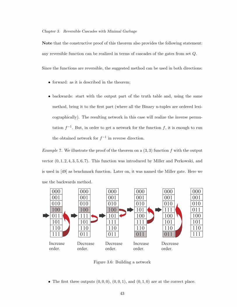
Chapter 3. Reversible Cascades with Minimal Garbage
Note that the constructive proof of this theorem also provides the following statement:
any reversible function can be realized in terms of cascades of the gates from set Q.
Since the functions are reversible, the suggested method can be used in both directions:
• forward: as it is described in the theorem;
• backwards: start with the output part of the truth table and, using the same
method, bring it to the first part (where all the Binary n-tuples are ordered lexi-
cographically). The resulting network in this case will realize the inverse permu-
tation f−1. But, in order to get a network for the function f , it is enough to run
the obtained network for f−1 in reverse direction.
Example 7. We illustrate the proof of the theorem on a (3, 3) function f with the output
vector (0, 1, 2, 4, 3, 5, 6, 7). This function was introduced by Miller and Perkowski, and
is used in [49] as benchmark function. Later on, it was named the Miller gate. Here we
use the backwards method.
000001010
011100
101110111
Increaseorder.
000001010
011
100
101110
111
Decreaseorder.
000001010
011
100101
110111
Decreaseorder.
000001010
011
101100
110111
Increaseorder.
000001010
011
111100
110101
Decreaseorder.
000001010
111
011100
110101
Figure 3.6: Building a network
• The first three outputs (0, 0, 0), (0, 0, 1), and (0, 1, 0) are at the correct place.
43
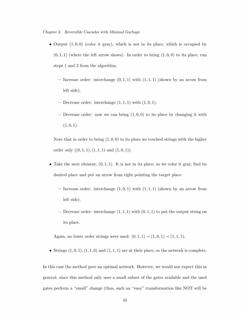
Chapter 3. Reversible Cascades with Minimal Garbage
• Output (1, 0, 0) (color it gray), which is not in its place, which is occupied by
(0, 1, 1) (where the left arrow shows). In order to bring (1, 0, 0) to its place, run
steps 1 and 2 from the algorithm.
– Increase order: interchange (0, 1, 1) with (1, 1, 1) (shown by an arrow from
left side).
– Decrease order: interchange (1, 1, 1) with (1, 0, 1).
– Decrease order: now we can bring (1, 0, 0) to its place by changing it with
(1, 0, 1).
Note that in order to bring (1, 0, 0) to its place we touched strings with the higher
order only ((0, 1, 1), (1, 1, 1) and (1, 0, 1)).
• Take the next element, (0, 1, 1). It is not in its place, so we color it gray, find its
desired place and put an arrow from right pointing the target place.
– Increase order: interchange (1, 0, 1) with (1, 1, 1) (shown by an arrow from
left side).
– Decrease order: interchange (1, 1, 1) with (0, 1, 1) to put the output string on
its place.
Again, no lower order strings were used: (0, 1, 1) ≺ (1, 0, 1) ≺ (1, 1, 1).
• Strings (1, 0, 1), (1, 1, 0) and (1, 1, 1) are at their place, so the network is complete.
In this case the method gave an optimal network. However, we would not expect this in
general, since this method only uses a small subset of the gates available and the used
gates perform a “small” change (thus, such an “easy” transformation like NOT will be
44

Chapter 3. Reversible Cascades with Minimal Garbage
realized by a large circuit). In addition, the theoretical method uses very wide gates,
thus the quantum complexity of the resulting circuit is expected to be very high. To
build a better circuits than the theoretical algorithm possibly can, we use a different
synthesis approach.
3.3 Heuristic Synthesis
Let Q be the set of all possible gates with n inputs. We have shown that |Q| = n3n−1.
Given the model for function implementation, the problem of synthesis is to write a
function in terms of a sequence of gates from the set Q.
We solve this problem using an incremental approach. That is, we repeatedly choose a
gate that will bring us closer to the desired function. In order to do this we need to be
able to measure how close two functions are, and we call this the distance between two
functions. We then choose the gate that will decrease the distance between the realized
function and the target function. We continue to do this until the distance is zero.
To give a formal definition of the distance, we need the following:
Definition 7. A partial realization of f is any function f ′ of the same set of variables.
Definition 8. The distance between a reversible function f and its partial realization
f ′ is the Hamming distance between the output parts of their truth tables.
Definition 9. The error of the function f is its distance to the identity function.
45
Chapter 3. Reversible Cascades with Minimal Garbage
Example 8. The reversible function f(x1, x2, x3) = (x1 ⊕ x2x3, x2, x1 ⊕ x2x3) whose
truth table is shown in Table 3.4 has 14 errors (shown in bold.)
x1 x2 x3 f1 f2 f3
0 0 0 0 1 0
0 0 1 1 1 0
0 1 0 0 0 0
0 1 1 0 0 1
1 0 0 1 1 1
1 0 1 0 1 1
1 1 0 1 0 1
1 1 1 1 0 0
Table 3.4: Truth table of f(x1, x2, x3) = (x1 ⊕ x2x3, x2, x1 ⊕ x2x3)
Example 9. A partial realization f ′(x1, x2, x3) = (x1 ⊕ x2x3, x2, x3) of the reversible
function from the previous example is at distance 12 from the target function f (see
Table 3.5.)
The previous two examples had an even number of error bits, and the number of error
1-bits was equal to the number of error 0-bits. This result holds in general as shown in
the following lemma.
Lemma 3. The error of a reversible function is even. Among the error bits the number
of those equal to one is the same as the number equal to zero.
Proof. To see that this is correct, we can write down the truth table of a reversible
46
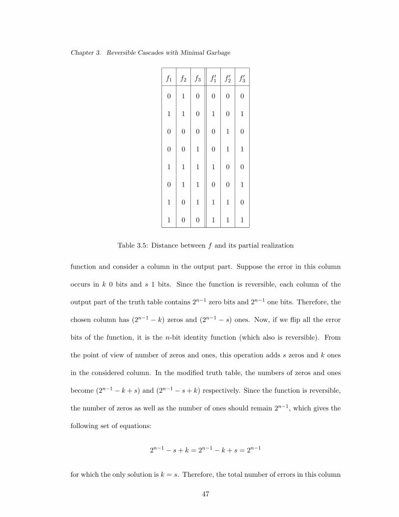
Chapter 3. Reversible Cascades with Minimal Garbage
f1 f2 f3 f ′1 f ′
2 f ′3
0 1 0 0 0 0
1 1 0 1 0 1
0 0 0 0 1 0
0 0 1 0 1 1
1 1 1 1 0 0
0 1 1 0 0 1
1 0 1 1 1 0
1 0 0 1 1 1
Table 3.5: Distance between f and its partial realization
function and consider a column in the output part. Suppose the error in this column
occurs in k 0 bits and s 1 bits. Since the function is reversible, each column of the
output part of the truth table contains 2n−1 zero bits and 2n−1 one bits. Therefore, the
chosen column has (2n−1 − k) zeros and (2n−1 − s) ones. Now, if we flip all the error
bits of the function, it is the n-bit identity function (which also is reversible). From
the point of view of number of zeros and ones, this operation adds s zeros and k ones
in the considered column. In the modified truth table, the numbers of zeros and ones
become (2n−1 − k + s) and (2n−1 − s + k) respectively. Since the function is reversible,
the number of zeros as well as the number of ones should remain 2n−1, which gives the
following set of equations:
2n−1 − s + k = 2n−1 − k + s = 2n−1
for which the only solution is k = s. Therefore, the total number of errors in this column
47

Chapter 3. Reversible Cascades with Minimal Garbage
is 2k, an even number. The same proof can be given for each of n output columns, thus
the total error is an even number. ¥
Note that we actually proved a stronger statement, namely: the error is an even number
in every output column. The other consequence we can derive is that the distance
between a function and its partial implementation is always an even number. It is also
not hard to see that the number of ones that are out of place is the same as the number
of zeros that are out of place.
Consider the following simple idea for a synthesis method, which it will be used later as
a basis for the heuristic synthesis algorithm we build: start with identity function, find
a gate from the set Q such that when added to the partial realization f ′ will decrease
the distance to f . Sometimes there is no gate that decreases the distance to f . But at
any time, it is possible to choose a gate that at least does not increase the distance to
f . For an illustration see Example 10.
Example 10. A reversible function with specification (x, y) → (y, x) and the identity
function, have this property: no gate will improve the distance function.
We use the word step to denote the addition of a gate to a cascade network. Therefore,
the number of steps made is the number of gates in the network. A step is called
positive (negative) if the distance increases (decreases).
Lemma 4. (existence of non-positive step) If the distance between f and f ′ is
greater than zero (the partial realization f ′ is not the function f itself yet), there exists
a gate in Q that transforms f ′ to f ′′ such that the distance between f and f ′′ is less
48

Chapter 3. Reversible Cascades with Minimal Garbage
than or equal to the distance between f and f ′.
Proof. Let (a1, a2, ..., an−1, X) be a string in the output part of the truth table of
some partial realization with an error in bit X (which is assumed to be on the n-th place
without loss of generality). Interchange it with the distance-1 string (a1, a2, ..., an−1, an),
where an = X. To do so use the gate made of line types 3 − a1, 3 − a2, ..., 3 − an−1, 1
correspondingly, where the Boolean numbers a1, a2, ..., an−1 are treated as natural num-
bers. It is easy to see that the gate with this specification exchanges the named strings
and does nothing to all others. Errors in the first (n-1) bits stay the same, but for the
last bit the following table shows all the possible ways this interchange could happen
(Table 3.6). So, we get a zero step or a negative step. ¥
X value an value an was correct? error was error becomes step is
0 1 Y 1 1 0
1 0 Y 1 1 0
0 1 N 2 0 -2
1 0 N 2 0 -2
Table 3.6: Effect of changing one bit
Here the question arises: is it possible to realize the function without positive steps?
The answer is yes, and the design method is given in Theorem 3. The proof for this
theorem is constructive and suggests a design procedure. The only thing that is left to
prove is that the steps “Increase order” and “Decrease order” are non-positive. Indeed,
the essence of each of these steps is to put a correct bit (0 for “Increase order” and 1 for
49
Chapter 3. Reversible Cascades with Minimal Garbage
“Decrease order” steps) in its place. The Lemma above states that each of these steps
are non-positive. This fact allows us to formulate the following result and use it as a
core to create a synthesis algorithm.
Theorem 4. There exists a synthesis method that adds a gate only if it performs a
non-positive change to the distance function. Such a method converges for any reversible
function.
3.3.1 The Algorithm
The actual implementation of the algorithm works as follows:
1. Define the number MaxMoves (which in actual implementations was taken in the
range of 50-500).
2. While the distance is greater than zero from among all Q gates, find the best
MaxMoves steps. For each of them, find the best second step. After this step
there are MaxMoves pairs of gates in the list. Search for the sequence of 2 gates
that maximally improves (minimizes) the distance between the existing partial
realization and the function itself. If such a pair is unique, attach the first gate to
the cascade and go back to 2.
3. If two or more pairs of gates produce the same improvement to the distance,
activate TieBreaker. TieBreaker is the function that finds the third best gate
for each pair, and if one of the pairs has a better third gate (that minimizes the
distance function), chooses this pair. Then, attach the first gate of the chosen pair
to the cascade and go to 2.
50

Chapter 3. Reversible Cascades with Minimal Garbage
4. If TieBreaker was not able to find a pair where the third step gives a better
improvement, then take the pair that gives the best improvement for the first
gate. Go to 2.
5. If the gate to be assigned is not chosen yet, take the first pair of the gates among
those that give the best improvement (from the list produced at step 2). Go to 2.
Theorem 4 states that the distance will not be increased, because there is always a zero
step available. In general such a method is not guaranteed to converge, although it does
converge for every function we tried. We use this algorithm instead of the theoretical
one that is guaranteed to converge, since the latter is likely to give a larger number of
steps, because the distance can only decrease by at most two.
An (n, n) reversible function (f1, f2, ..., fn) in general can be realized by one of the n!
possible designs. This happens if we assume that the order of the output functions does
not matter. We can enumerate the outputs in any order, and thusly realize different
functions. In our case, for the larger functions (starting from (7,7) functions and larger)
we used a heuristic for the output permutation: we took the output permutation that
gave the smallest error for the function or its complement. For the functions with a
smaller number of variables, we are able to run all the possible permutations and choose
the best result.
Example 11. Consider the function with specification (x, y) → (y, x) from Example 10.
Without the output permutation it will take us at least three gates to build a network
for it: the first step is a zero step, as was shown in the previous example. Then, we
have 2 errors in each of two output bits. This will require at least 2 more gates, since
51
Chapter 3. Reversible Cascades with Minimal Garbage
each of them in the best case scenario can take care of at most one output bit at a time.
So, the theoretical minimum is 3 gates (in fact, our algorithm terminates in 3 steps). A
function (x, y) → (y, x) with permuted outputs (that is, (x, y) → (x, y)) can be easily
realized with two steps, namely a negation of first and second input bits.
3.3.2 Multiple Output Functions
Using the results of Theorem 1 we are able to add the minimal number of garbage bits
in order to make a multiple output function reversible. The benefit in realization of a
multiple output function is that we do not care about some of the outputs; the actual
values of the garbage bits are of no interest. This allows us to:
1. Have a smaller error and therefore, in general, have less steps to make in order to
create a network.
2. Have more freedom in changing “don’t care” outputs. There is no risk in adding
an error to a “don’t care” output. We minimize the distance to the target outputs
only.
3.3.3 Benchmarks
Due to the similarity of gates in the set Q and the generalized Toffoli gates, we introduce
the following notation. The gate Qa1,a2,...,an is denoted as TOF(xσ1i1
, xσ2i2
, ..., xσs−1
is−1; y),
which is constructed as follows:
• Write “TOF(”.
• For each ai
– if ai = 2 write “xi”;
52
Chapter 3. Reversible Cascades with Minimal Garbage
– if ai = 3 write “xi”;
– otherwise do nothing.
Separate different entities with commas.
• Write “; xj” at the very end, where j is defined such that aj = 1. By the definition
of Q gate such j will be unique. Finish with the closing bracket “)”.
For example, gate Q3,1,4,2,4 can also be written as TOF(x1, x4; x2). This form of writing
the gate is better for application use since it makes sense out of the structure of a gate.
The old form was used for the simplicity of formulas in mathematical proofs.
In this section we compare our algorithm to the previous algorithms. Unfortunately,
some authors do not give enough information to allow us to do so. For example, authors
of [29] suggest an approach for reversible cascade synthesis of one output functions.
They do not provide the experimental results, nor the algorithm, therefore we can not
compare those results to ours. Shende et al. [74, 75] provide the optimal synthesis
method for the (3, 3) reversible functions only. Work [60] is concentrated on reversible
synthesis of symmetric functions, which is less general than our approach. Iwama et al.
[22] base their method on circuit transforms, but they do not provide any experimental
data.
We compare our results with those of three systematic methods: one by Miller [49],
another by Mishchenko and Perkowski [54], and a third by Khan and Perkowski [28, 27].
Miller [49] suggests a reversible function synthesis that starts with a reversible specifi-
cation only. He uses a spectral technique to find the best gate to be added in terms of
53

Chapter 3. Reversible Cascades with Minimal Garbage
gates (NOT, CNOT, Toffoli3, and Toffoli4) and adds the gate in a cascade-like manner.
This method has been modified in [50] to synthesize networks of the presented RCMG
model. In his method the output function is required to appear as a set of actual outputs
or their negations. Miller also used a postprocessing process to simplify the network
(the results of simplification are given in brackets for the cases for which the process
was done). The results from all examples in [49] compared to ours are summarized in
Table 3.7, where name is the name of the benchmark function, in/out is the number
of its inputs/outputs, Miller is the number of gates for Miller’s method, and We is the
number of gates for the proposed synthesis method.
name in/out Miller We
ex1 3 3 3
ex2 3 5 5
ex3 4 7 7
ex4 3 4 3
ex5 4 5 4
ex6 4 12(10) 7
ex7 4 9(7) 7
Table 3.7: Comparison with Miller’s results
Example 12. Since our method gives a better result for ex4, here follows our net-
work for this function. Ex4 is a (4, 4) reversible function, given as the truth vec-
tor [3, 11, 2, 10, 0, 7, 1, 6, 15, 8, 14, 9, 13, 5, 12, 4] whose binary representation gives the ac-
tual Boolean values. Using the output permutation (2, 1, 3, 4), the scheme consists of
54

Chapter 3. Reversible Cascades with Minimal Garbage
the following seven gates: TOF(b) TOF(c, d; a) TOF(a, d; c) TOF(a, c; d) TOF(c, d; a)
TOF(a, d; c) TOF(a, c; b) for the names of variables a, b, c and d. In comparison, Miller’s
synthesized network is: TOF(d) TOF(b) TOF(b, c; d) TOF(b) TOF(a, c; d) TOF(c)
TOF(a, b; d) TOF(a; c) TOF(b, c; a) TOF(b; c) TOF(a; c) TOF(a; b). This network was
transformed to the following: TOF(d) TOF(b) TOF(b, c; d) TOF(b) TOF(a, c; d) TOF(c)
TOF(a, b; d) FRE(b, c; a) TOF(b; c) TOF(a; b), where FRE(b, c; a) is the Fredkin gate.
Mishchenko and Perkowski [54] suggest a reversible wave cascade method and evaluate
the complexity of some benchmark functions in terms of the number of these cascades.
They do not provide the actual design for the described method, but instead they give
upper bounds. We compare their results to ours and summarize the comparison in Table
3.8. Although our results are not always better than those of Mishchenko and Perkowski
in terms of the total complexity, the important factor, the number of garbage bits, is
definitely improved using our approach. We were not able to compare the results for
functions with a larger number of inputs/outputs due to the huge amount of work our
algorithm needs to find a network representing such a function. In this table, the first
Function Garbage Cost
name in out Mishchenko, Perkowski We Mishchenko, Perkowski We
5xp1 7 10 38 0 31 43
9sym 9 1 56 9 52 60
rd53 5 3 19 4 14 13
rd73 7 3 43 6 36 36
Table 3.8: Comparison with Perkowski’s results
55

Chapter 3. Reversible Cascades with Minimal Garbage
three columns describe the function: the name, number of input bits, and number of out-
put bits of a benchmark function. First pair of columns Mishchenko-Perkowski and
We lists the number of garbage outputs from the result of Mishchenko and Perkowski’s
method and our method; the remaining pair of columns compares the numbers of gates
in designs of the benchmark functions for Mishchenko and Perkowski’s method and our
proposed design respectively. Our method does not always find the realization with the
minimum number of gates, but if we consider the cost of a benchmark function to be
the sum of the number of gates and the garbage, then our method gives a better result.
Results shown by Khan [28, 27] are weaker (although newer) than the results in [54], but
for the sake of completeness, we show the comparison in the table below. Note that our
results are better in all cases except for the 9sym function. However, this is a weakness
of the synthesis method we have, not the model, since every single output non-balanced
function can be realized with the cost of the number of terms in its minimal EXOR
polynomial as is shown in Section 3.4 of this chapter.
Function Garbage Cost
name in out Khan We Khan We
5xp1 7 10 63 0 56 49
9sym 9 1 60 9 52 56
rd53 5 3 19 4 17 13
rd73 7 3 47 6 43 36
Table 3.9: Comparison with Khan’s results
56

Chapter 3. Reversible Cascades with Minimal Garbage
It is also interesting to notice that the benchmark rd53 can be realized in terms of
an ESOP with 14 terms as the result of Perkowski and Mishchenko states. For our
method this number is 13, which shows that the proposed method can do better than
EXOR minimization can. The following example contains one more function for which
our method is more efficient, compared to the standard non-reversible technological
realization of ESOP, the EXOR PLA.
Example 13. The (5, 1)-function 2of5 whose output is 1 if and only if exactly two of
the input variables are 1 in terms of ESOP can be realized with 8 terms. Our synthesis
method is capable of creating a network (for the proposed structure) with 7 gates only.
The function 2of5 is not balanced, therefore the minimal garbage for it is 5. Thus,
the (5, 1)-function becomes a (6, 6) reversible function. We used the last output to
realize the function, and named the inputs as a, b, c, d, e, and f , where the last input
is a constant 0. The network structure is as follows: TOF(a, d, e, f ; c) TOF(b, c, d; f)
TOF(a, c, e; f) TOF(a, b, d, e; f) TOF(a, f ; e) TOF(b, c, d, e; f) TOF(b, c, d, e; f).
Some of the actual circuit designs that we discussed in this chapter can be viewed
at http : //www.cs.unb.ca/profs/gdueck/quantum/ [44]. It also happens that the
synthesis in RCMG model is beneficial to the synthesis of ESOPs, which is shown in
the following section.
3.4 RCMG and ESOP Comparison
To exploit the similarity between the two chosen models, note that each of the terms in
the ESOP can be treated as a separate gate. All the terms are arranged in the form of a
cascade, namely a string that is the EXOR of terms which builds the ESOP polynomial.
57
Chapter 3. Reversible Cascades with Minimal Garbage
The following summarizes the similarities and differences between the two models.
• Both models use the same operations, namely, AND, EXOR, and negation.
• The gates are similar. Each gate acts as an EXOR of the term built from the
input variables. The difference is that in ESOP the set of input variables is not
changing while passing through the gates, where for RCMG this is not true.
• The number of distinct gates is comparable: n ∗ 3n−1 for RCMG and 3n for the
ESOP.
• The gates are in a linear order. The terms being “exored” form a string, and
generalized Toffoli gates form a cascade. The difference between them is in whether
the order matters. The order of terms in a polynomial does not matter, whereas
the order of reversible gates in our model does.
Lemma 5. By adding a constant input it is possible to use the results of an ESOP
minimization to build a reversible network for a single output Boolean function.
Proof. Take an n-input Boolean function and create a zero constant on the input
line xn+1. This may result in non-optimality of the garbage. Transform each term
xσ1i1
xσ2i2
...xσkik
to the gate TOF (xσ1i1
, xσ2i2
, ..., xσkik
; xn+1). Such a transformation of each of
the terms in the ESOP results in the set of gates of the RCMG; when arranged in a
cascade, they form a reversible network for the function. ¥
The more interesting question is if the RCMG model is sufficiently efficient in comparison
to the ESOP. The answer for this question is “yes”, and the following set of Boolean
functions grows polynomially for the RCMG and exponentially for the ESOP.
58
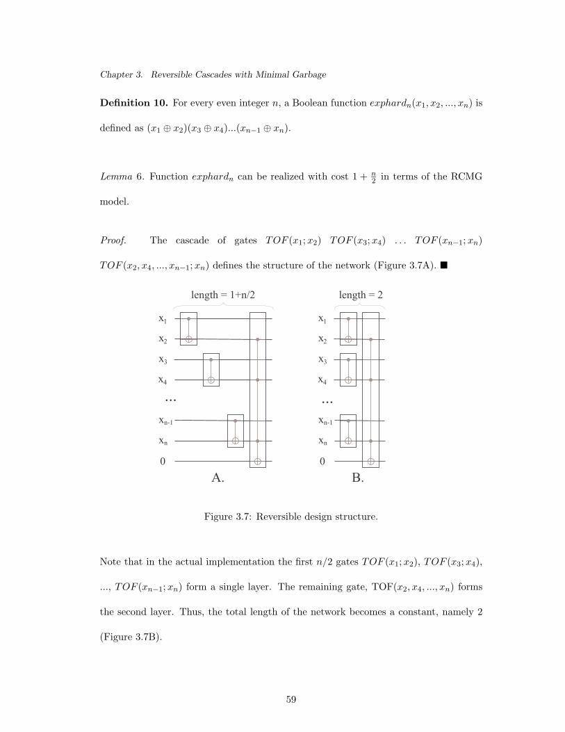
Chapter 3. Reversible Cascades with Minimal Garbage
Definition 10. For every even integer n, a Boolean function exphardn(x1, x2, ..., xn) is
defined as (x1 ⊕ x2)(x3 ⊕ x4)...(xn−1 ⊕ xn).
Lemma 6. Function exphardn can be realized with cost 1 + n2 in terms of the RCMG
model.
Proof. The cascade of gates TOF (x1; x2) TOF (x3; x4) . . . TOF (xn−1; xn)
TOF (x2, x4, ..., xn−1; xn) defines the structure of the network (Figure 3.7A). ¥
x
x
x
x
x
1
2
3
4
n-1
xn
0A.
length = 1+n/2
x
x
x
x
x
1
2
3
4
n-1
xn
0B.
length = 2
......
Figure 3.7: Reversible design structure.
Note that in the actual implementation the first n/2 gates TOF (x1; x2), TOF (x3; x4),
..., TOF (xn−1; xn) form a single layer. The remaining gate, TOF(x2, x4, ..., xn) forms
the second layer. Thus, the total length of the network becomes a constant, namely 2
(Figure 3.7B).
59
Chapter 3. Reversible Cascades with Minimal Garbage
To show that no ESOP shorter than an ESOP with exponential length can represent
function exphardn, we need the following Lemmas:
Lemma 7. Every term in an optimal ESOP for g(x1, x2, ..., xn, y) = yf(x1, x2, ..., xn),
where y 6∈ {x1, x2, ..., xn}, contains variable y and contains it without negation.
Proof. Let M be an optimal ESOP for the function g(x1, x2, ..., xn, y). Write it as
M = yM ′1 ⊕ M ′
2 ⊕ yM ′3 = y(M ′
1 ⊕ M ′3) ⊕ (M ′
2 ⊕ M ′3), (3.1)
where M ′1, M
′2 and M ′
3 do not contain y. The total cost of this ESOP is the sum of the
number of terms in M ′1, M
′2 and M ′
3, which is |M ′1| + |M ′
2| + |M ′3|. Let N be an ESOP
for f . Then yN forms an ESOP for yf . Add yN and M :
0 = yf ⊕ yf = yN ⊕ M = y(M ′1 ⊕ M ′
3 ⊕ N) ⊕ (M ′2 ⊕ M ′
3).
If we write it by components, we have:
M ′1 ⊕ M ′
3 ⊕ N = 0, M ′2 ⊕ M ′
3 = 0. (3.2)
Use this last equality to continue from equation (3.1):
yf = M = y(M ′1 ⊕ M ′
3) ⊕ (M ′2 ⊕ M ′
3)
= y(M ′1 ⊕ M ′
3) ⊕ 0
= y(M ′1 ⊕ M ′
3)
= yM ′1 ⊕ yM ′
3.
This ESOP has |M ′1| + |M ′
3| terms. Since M is minimal, the number of terms of M ′2 is
zero. Therefore, the number of terms of M ′3 is also zero, which can be seen from the
second equation in (3.2). In other words, M = yM ′1. ¥
60
Chapter 3. Reversible Cascades with Minimal Garbage
Lemma 8. Any optimal ESOP for g(x1, x2, ..., xn, y) = yf(x1, x2, ..., xn), where y 6∈
{x1, x2, ..., xn}, has the same complexity as an optimal ESOP for f(x1, x2, ..., xn).
Proof. Lemma 7 enables us to factor variable y out of an optimal ESOP M for the
function g(x1, x2, ..., xn, y): M = yM ′, where M ′ is an ESOP that does not contain y in
any form. Let y = 1. Then, M ′ = (yM ′)|y=1 = M |y=1 = (yf(x1, x2, ..., xn))|y=1 =
f(x1, x2, ..., xn). In other words, M ′ has the complexity of a minimal ESOP for
f(x1, x2, ..., xn), so the ESOP M does also. ¥
Lemma 9. A minimal ESOP for the function g(x1, x2, ..., xn, y, z) = yf(x1, x2, ..., xn)⊕
zf(x1, x2, ..., xn), where y, z are variables and y, z 6∈ {x1, x2, ..., xn}, consists of at least
3|f |2 terms, where |f | is the number of terms in a minimal ESOP for f .
Proof. We can take a minimal ESOP M of the function g(x1, x2, ..., xn, y, z) and write
it as M = yM1 ⊕ M2 ⊕ yM3, where M1, M2 and M3 are ESOPs that do not contain
the variable y in either term. Such a decomposition is unique. Notice that the sets of
terms in each of M1, M2 and M3 do not intersect:
• M1 ∩ M2 = ∅;
• M1 ∩ M3 = ∅;
• M2 ∩ M3 = ∅.
Otherwise, suppose that M1 ∩M2 6= ∅. Then, there exists a term t ∈ (M1 ∩M2). Since
yt ⊕ t = yt, by deleting these two terms from ESOPs M1 and M2 and adding it to
M3 we get an ESOP that has complexity (that is, the number of terms in an ESOP)
61

Chapter 3. Reversible Cascades with Minimal Garbage
one less than the optimal ESOP M . This contradicts the optimality of M . Therefore,
M1 ∩ M2 = ∅. The other two set intersections can be proven to be empty similarly.
Let y = 0 in the ESOP M = yM1 ⊕M2 ⊕ yM3 for the function yf ⊕ zf . This results in
(yf ⊕ zf)|y=0 = (yM1 ⊕ M2 ⊕ yM3)|y=0
and
zf = M2 ⊕ M3. (3.3)
Similarly, assigning y = 1 leads to
zf = M1 ⊕ M2. (3.4)
Adding (3.3) and (3.4) produces
f = M1 ⊕ M3. (3.5)
By Lemma 8, we conclude that each of the ESOPs in (3.3) and (3.4) has at least |f |
terms. So does the ESOP from (3.5).
As we proved before, the sets of terms in M1, M2 and M3 do not intersect, so based on
Lemma 8, (3.3), (3.4), and (3.5), the following system can be written:
|M2 ⊕ M3| = |M2| + |M3| ≥ |f |
|M1 ⊕ M2| = |M1| + |M2| ≥ |f |
|M1 ⊕ M3| = |M1| + |M3| ≥ |f |
.
Since
|M | = |yM1 ⊕ M2 ⊕ yM3| = |M1| + |M2| + |M3|,
62
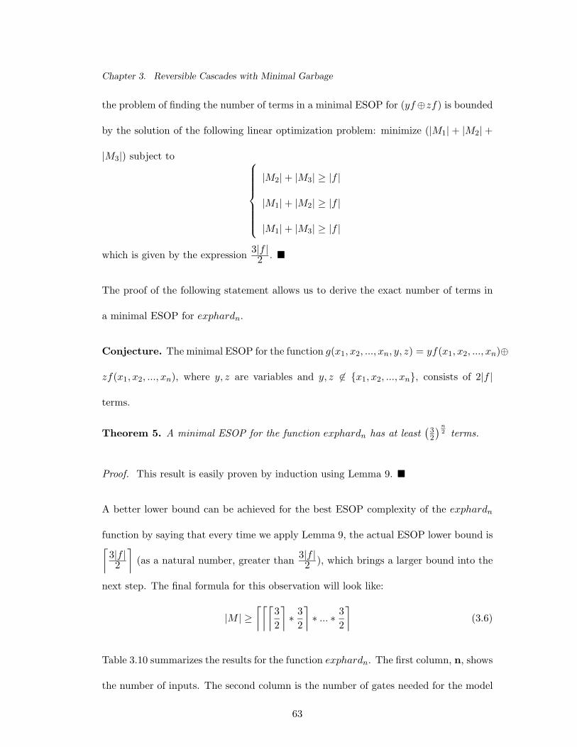
Chapter 3. Reversible Cascades with Minimal Garbage
the problem of finding the number of terms in a minimal ESOP for (yf⊕zf) is bounded
by the solution of the following linear optimization problem: minimize (|M1| + |M2| +
|M3|) subject to
|M2| + |M3| ≥ |f |
|M1| + |M2| ≥ |f |
|M1| + |M3| ≥ |f |
which is given by the expression 3|f |2 . ¥
The proof of the following statement allows us to derive the exact number of terms in
a minimal ESOP for exphardn.
Conjecture. The minimal ESOP for the function g(x1, x2, ..., xn, y, z) = yf(x1, x2, ..., xn)⊕
zf(x1, x2, ..., xn), where y, z are variables and y, z 6∈ {x1, x2, ..., xn}, consists of 2|f |
terms.
Theorem 5. A minimal ESOP for the function exphardn has at least(
32
)n2 terms.
Proof. This result is easily proven by induction using Lemma 9. ¥
A better lower bound can be achieved for the best ESOP complexity of the exphardn
function by saying that every time we apply Lemma 9, the actual ESOP lower bound is⌈3|f |2
⌉(as a natural number, greater than 3|f |
2 ), which brings a larger bound into the
next step. The final formula for this observation will look like:
|M | ≥⌈⌈⌈
32
⌉∗ 3
2
⌉∗ ... ∗ 3
2
⌉(3.6)
Table 3.10 summarizes the results for the function exphardn. The first column, n, shows
the number of inputs. The second column is the number of gates needed for the model
63
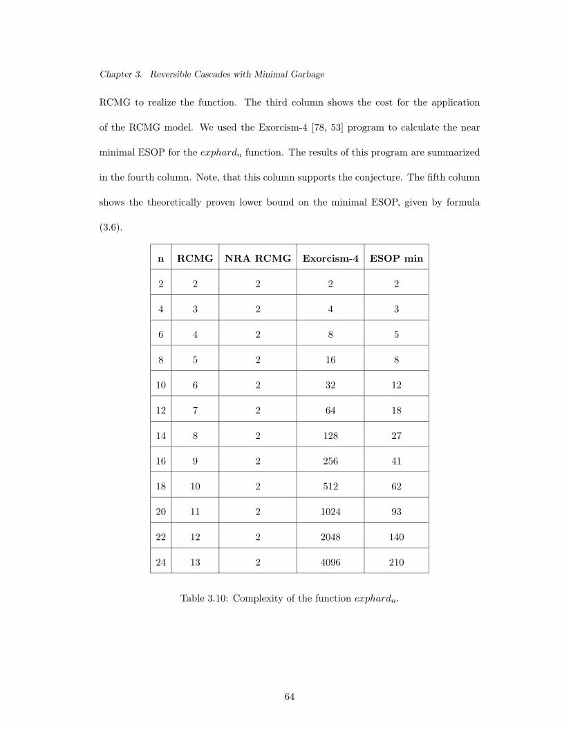
Chapter 3. Reversible Cascades with Minimal Garbage
RCMG to realize the function. The third column shows the cost for the application
of the RCMG model. We used the Exorcism-4 [78, 53] program to calculate the near
minimal ESOP for the exphardn function. The results of this program are summarized
in the fourth column. Note, that this column supports the conjecture. The fifth column
shows the theoretically proven lower bound on the minimal ESOP, given by formula
(3.6).
n RCMG NRA RCMG Exorcism-4 ESOP min
2 2 2 2 2
4 3 2 4 3
6 4 2 8 5
8 5 2 16 8
10 6 2 32 12
12 7 2 64 18
14 8 2 128 27
16 9 2 256 41
18 10 2 512 62
20 11 2 1024 93
22 12 2 2048 140
24 13 2 4096 210
Table 3.10: Complexity of the function exphardn.
64
Chapter 3. Reversible Cascades with Minimal Garbage
3.4.1 Multiple Output Functions
One of the reasons that ESOPs are used is their ability to share terms. The RCMG
model does not have this property. However, the RCMG model can be united with the
mEXOR model introduced in Chapter 6 to form a new hybrid model. This will allow the
use of multiple EXOR output Toffoli gates with the same control, which is equivalent
to term sharing in the non-reversible ESOP model. It can be shown by examining the
gate that the quantum realization of such a hybrid gate has a cost that differs from the
cost of the original Toffoli gate only marginally, e.g. around 10%. The result of Lemma
5 will now hold for any multiple output Boolean function.
3.5 Conclusions
In this chapter we introduced the synthesis model and the synthesis procedure which
allows us to minimize the most important factor of the reversible circuit cost (for in-
stance, for quantum NMR technology) — its garbage. We showed that the new gates
differ from the generalized Toffoli gates only marginally. We synthesized the benchmark
functions and achieved good results in comparison to the previously shown results: in
some cases our method requires less gates, and in all cases our garbage is theoretically
minimal. Finally, the synthesis in the RCMG model was shown to be better in compar-
ison to the synthesis of conventional ESOPs in the sense that no RCMG representation
of a function requires more gates than the number of terms in a minimal ESOP. On the
other hand, there exists a class of polynomial complexity functions in terms of RCMG
which can be realized as an ESOP with exponential cost only.
65

Chapter 4Toffoli Synthesis
The RCMG model from the previous section has used complex gates, which essentially
consist of three logical parts: NOT gate preprocessing, a generalized Toffoli gate, and
NOT gate postprocessing. One of the unavoidable problems of this theoretical algo-
rithm discussed in the previous chapter, and a reason to create a different heuristic
procedure, is the number and size of the gates needed for the computation. Clearly, it
is better to have fewer gates of a smaller size. In this chapter this problem is solved by
considering Toffoli gates and an updated synthesis procedure, which tries to use narrow
(with less controls) gates. This new synthesis algorithm keeps the key idea presented
in the previous section; initially the cascade is built from the outputs to the inputs,
by bringing patterns to their places without changing patterns which are already at
their place. Furthermore, a generalized version of this algorithm, a bidirectional modi-
fication, is developed. When the algorithm terminates and an initial circuit is created,
local transformations, called template simplification tools, are applied. In this chapter
we do not concentrate on results, since in Chapter 5, the algorithm and template tools
are generalized to handle Toffoli and Fredkin gates, so the results of this chapter will
be covered by newer results in Chapter 5. Toffoli templates are of interest as they are
easier to analyze, and develop our intuition for a more generalized set of templates.
66
Chapter 4. Toffoli Synthesis
4.1 The Algorithm
Applying a Toffoli gate to the inputs or outputs of a reversible function always yields a
reversible function. The synthesis problem is to find a sequence of Toffoli gates which
transforms a given reversible function to the identity function. As gates can be applied
either to the inputs or outputs, the synthesis can proceed from outputs to inputs, from
inputs to outputs or, as we show in Subsection 4.1.2, in both directions simultaneously.
4.1.1 Basic Algorithm
To begin, we present a basic naive and greedy algorithm which identifies Toffoli gates
only on the output side of the specification.
Consider a reversible function specified as a mapping over {0, 1, ..., 2n − 1}; in other
words, a truth vector.
Basic Algorithm
Step 0: If f(0) 6= 0, invert the outputs corresponding to 1-bits in f(0). Each inversion
requires a NOT gate. The transformed function f+ has f+(0) = 0.
Step i: Consider each i in turn for 1 ≤ i < 2n − 1 letting f+ denote the current
reversible specification. If f+(i) = i, no transformation and hence no Toffoli gate is
required for this i. Otherwise, gates are required to transform the specification to a new
specification with f++(i) = i. The required gates must map f+(i) → i.
Let p be the bit string with 1s in all positions where the binary expansion of i is 1 while
the expansion of f+(i) is 0. These are the 1 bits that must be added in transforming
67
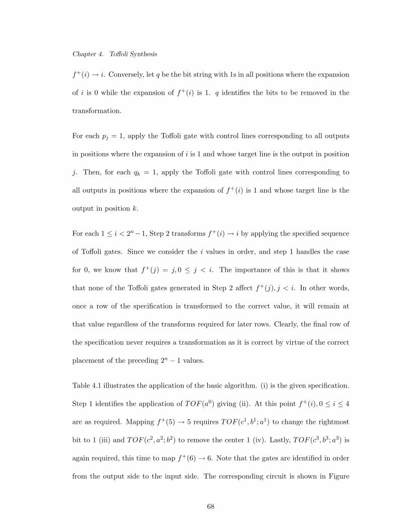
Chapter 4. Toffoli Synthesis
f+(i) → i. Conversely, let q be the bit string with 1s in all positions where the expansion
of i is 0 while the expansion of f+(i) is 1. q identifies the bits to be removed in the
transformation.
For each pj = 1, apply the Toffoli gate with control lines corresponding to all outputs
in positions where the expansion of i is 1 and whose target line is the output in position
j. Then, for each qk = 1, apply the Toffoli gate with control lines corresponding to
all outputs in positions where the expansion of f+(i) is 1 and whose target line is the
output in position k.
For each 1 ≤ i < 2n−1, Step 2 transforms f+(i) → i by applying the specified sequence
of Toffoli gates. Since we consider the i values in order, and step 1 handles the case
for 0, we know that f+(j) = j, 0 ≤ j < i. The importance of this is that it shows
that none of the Toffoli gates generated in Step 2 affect f+(j), j < i. In other words,
once a row of the specification is transformed to the correct value, it will remain at
that value regardless of the transforms required for later rows. Clearly, the final row of
the specification never requires a transformation as it is correct by virtue of the correct
placement of the preceding 2n − 1 values.
Table 4.1 illustrates the application of the basic algorithm. (i) is the given specification.
Step 1 identifies the application of TOF (a0) giving (ii). At this point f+(i), 0 ≤ i ≤ 4
are as required. Mapping f+(5) → 5 requires TOF (c1, b1; a1) to change the rightmost
bit to 1 (iii) and TOF (c2, a2; b2) to remove the center 1 (iv). Lastly, TOF (c3, b3; a3) is
again required, this time to map f+(6) → 6. Note that the gates are identified in order
from the output side to the input side. The corresponding circuit is shown in Figure
68
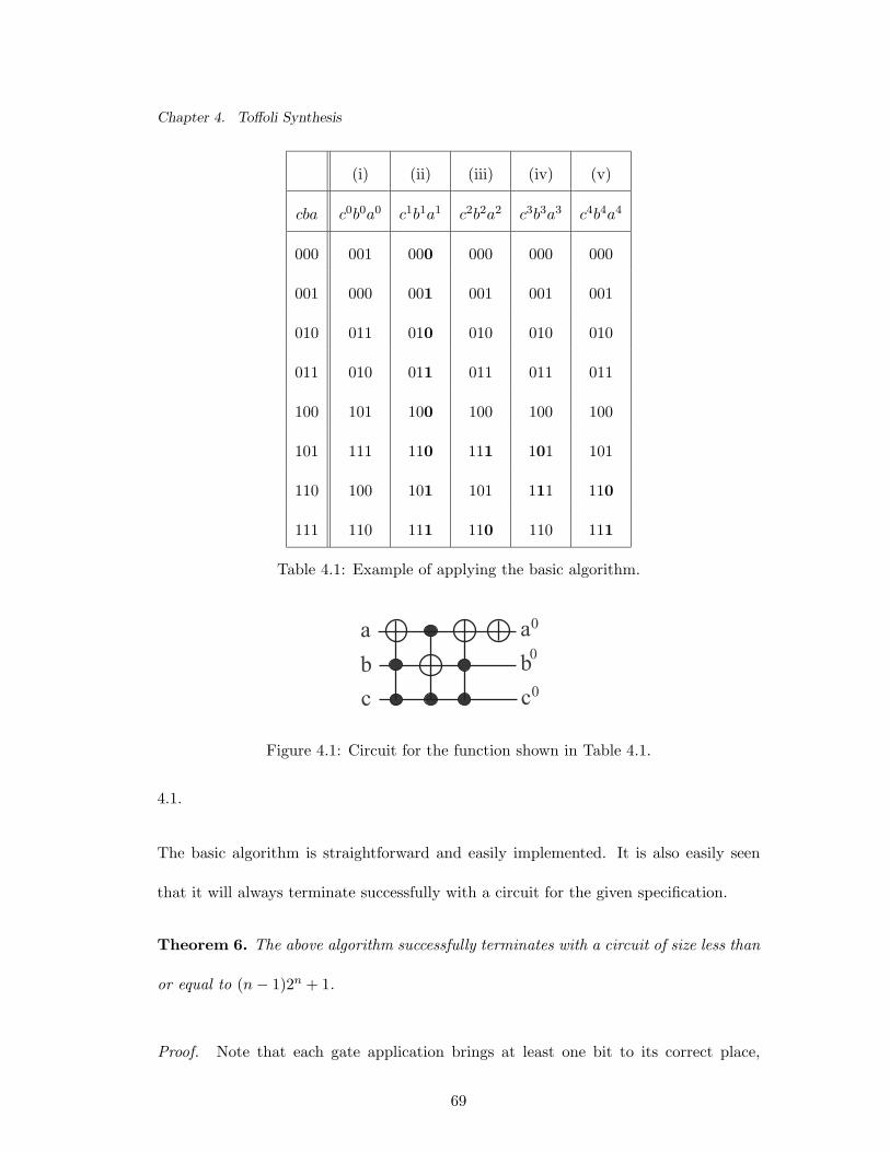
Chapter 4. Toffoli Synthesis
(i) (ii) (iii) (iv) (v)
cba c0b0a0 c1b1a1 c2b2a2 c3b3a3 c4b4a4
000 001 000 000 000 000
001 000 001 001 001 001
010 011 010 010 010 010
011 010 011 011 011 011
100 101 100 100 100 100
101 111 110 111 101 101
110 100 101 101 111 110
111 110 111 110 110 111
Table 4.1: Example of applying the basic algorithm.
abc
abc
0
0
0
Figure 4.1: Circuit for the function shown in Table 4.1.
4.1.
The basic algorithm is straightforward and easily implemented. It is also easily seen
that it will always terminate successfully with a circuit for the given specification.
Theorem 6. The above algorithm successfully terminates with a circuit of size less than
or equal to (n − 1)2n + 1.
Proof. Note that each gate application brings at least one bit to its correct place,
69
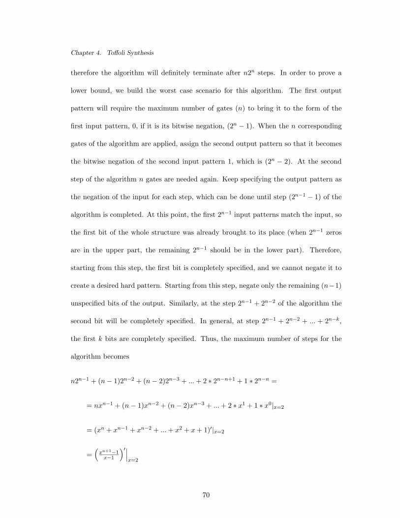
Chapter 4. Toffoli Synthesis
therefore the algorithm will definitely terminate after n2n steps. In order to prove a
lower bound, we build the worst case scenario for this algorithm. The first output
pattern will require the maximum number of gates (n) to bring it to the form of the
first input pattern, 0, if it is its bitwise negation, (2n − 1). When the n corresponding
gates of the algorithm are applied, assign the second output pattern so that it becomes
the bitwise negation of the second input pattern 1, which is (2n − 2). At the second
step of the algorithm n gates are needed again. Keep specifying the output pattern as
the negation of the input for each step, which can be done until step (2n−1 − 1) of the
algorithm is completed. At this point, the first 2n−1 input patterns match the input, so
the first bit of the whole structure was already brought to its place (when 2n−1 zeros
are in the upper part, the remaining 2n−1 should be in the lower part). Therefore,
starting from this step, the first bit is completely specified, and we cannot negate it to
create a desired hard pattern. Starting from this step, negate only the remaining (n−1)
unspecified bits of the output. Similarly, at the step 2n−1 + 2n−2 of the algorithm the
second bit will be completely specified. In general, at step 2n−1 + 2n−2 + ... + 2n−k,
the first k bits are completely specified. Thus, the maximum number of steps for the
algorithm becomes
n2n−1 + (n − 1)2n−2 + (n − 2)2n−3 + ... + 2 ∗ 2n−n+1 + 1 ∗ 2n−n =
= nxn−1 + (n − 1)xn−2 + (n − 2)xn−3 + ... + 2 ∗ x1 + 1 ∗ x0|x=2
= (xn + xn−1 + xn−2 + ... + x2 + x + 1)′|x=2
=(
xn+1−1x−1
)′∣∣∣x=2
70

Chapter 4. Toffoli Synthesis
=(
(n+1)xn(x−1)−xn+1+1(x−1)2
)∣∣∣x=2
=(
(n+1)2n(2−1)−2n+1+1(2−1)2
)
= (n + 1)2n − 2n+1 + 1 = (n − 1)2n + 1.
¥
Using the procedure from Theorem 6, it is possible to construct a (unique) function
for any n that requires (n − 1)2n + 1 gates. Therefore, the upper bound is tight.
For n = 3, this function has the truth vector [7, 1, 4, 3, 0, 2, 6, 5] and will be further
referred as 3 17. Using Theorem 6, it can be calculated that its cost is (3 − 1)23 + 1 =
2 ∗ 8 + 1 = 17, which explains the given name: 3 represents the size and 17 represents
the algorithm cost. Analogously, 4 49 is a size 4 hard function, whose truth vector is
[15, 1, 12, 3, 5, 6, 8, 7, 0, 10, 13, 9, 2, 4, 14, 11]. Functions with a larger number of variables
can be built. We will simplify the networks further and consider these functions to
measure how good the simplification is.
We next consider a bidirectional algorithm, which usually produces smaller circuits.
4.1.2 Bidirectional Algorithm
As described so far, the algorithm produces the circuit by selecting the Toffoli gates
that manipulate only the output side of the specification. Since the specification is
reversible, one could consider the inverse specification, derive a reverse circuit, and then
choose whichever is smaller. A better approach is to apply the method in both directions
simultaneously choosing to add gates at the input side or the output side.
71
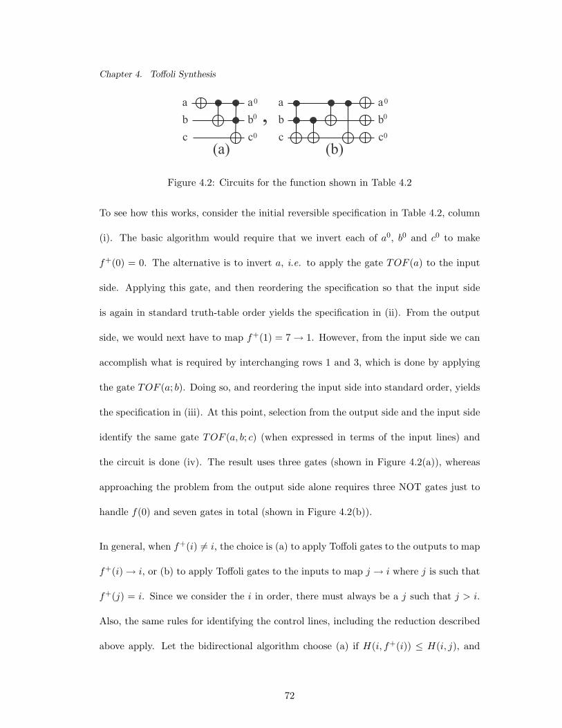
Chapter 4. Toffoli Synthesis
abc
,(a) (b)
0
0
0
abc
abc
0
0
0
abc
Figure 4.2: Circuits for the function shown in Table 4.2
To see how this works, consider the initial reversible specification in Table 4.2, column
(i). The basic algorithm would require that we invert each of a0, b0 and c0 to make
f+(0) = 0. The alternative is to invert a, i.e. to apply the gate TOF (a) to the input
side. Applying this gate, and then reordering the specification so that the input side
is again in standard truth-table order yields the specification in (ii). From the output
side, we would next have to map f+(1) = 7 → 1. However, from the input side we can
accomplish what is required by interchanging rows 1 and 3, which is done by applying
the gate TOF (a; b). Doing so, and reordering the input side into standard order, yields
the specification in (iii). At this point, selection from the output side and the input side
identify the same gate TOF (a, b; c) (when expressed in terms of the input lines) and
the circuit is done (iv). The result uses three gates (shown in Figure 4.2(a)), whereas
approaching the problem from the output side alone requires three NOT gates just to
handle f(0) and seven gates in total (shown in Figure 4.2(b)).
In general, when f+(i) 6= i, the choice is (a) to apply Toffoli gates to the outputs to map
f+(i) → i, or (b) to apply Toffoli gates to the inputs to map j → i where j is such that
f+(j) = i. Since we consider the i in order, there must always be a j such that j > i.
Also, the same rules for identifying the control lines, including the reduction described
above apply. Let the bidirectional algorithm choose (a) if H(i, f+(i)) ≤ H(i, j), and
72
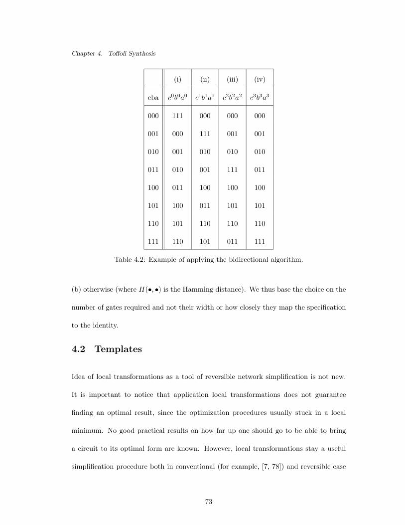
Chapter 4. Toffoli Synthesis
(i) (ii) (iii) (iv)
cba c0b0a0 c1b1a1 c2b2a2 c3b3a3
000 111 000 000 000
001 000 111 001 001
010 001 010 010 010
011 010 001 111 011
100 011 100 100 100
101 100 011 101 101
110 101 110 110 110
111 110 101 011 111
Table 4.2: Example of applying the bidirectional algorithm.
(b) otherwise (where H(•, •) is the Hamming distance). We thus base the choice on the
number of gates required and not their width or how closely they map the specification
to the identity.
4.2 Templates
Idea of local transformations as a tool of reversible network simplification is not new.
It is important to notice that application local transformations does not guarantee
finding an optimal result, since the optimization procedures usually stuck in a local
minimum. No good practical results on how far up one should go to be able to bring
a circuit to its optimal form are known. However, local transformations stay a useful
simplification procedure both in conventional (for example, [7, 78]) and reversible case
73
Chapter 4. Toffoli Synthesis
[22, 74, 42, 51, 75, 43, 41].
Several authors considered reversible network transformations. Shende et. al [74, 75]
used several 4-bit circuit equivalences to be able to rewrite gates in a different order.
Iwama, Kambayashi, and Yamashita [22] introduced some circuit transformation rules,
which mainly served to bring a network to a canonical form and thus, stating that the
set of transforms is complete. One of the transforms in [22] was proposed for circuit
simplification, but the actual application procedure was not described.
In [51], templates were introduced as a tool for network simplification. In that work, a
template consists of two sequences of gates which realize the same function. The first
sequence of gates is to be matched to a part of the circuit being simplified and the
second sequence is to be substituted when a match is found. The templates in Figure
4.3 were identified and classified based on their similarity: the first number in the figure
shows which class the given template belongs to, the second identifies ordinal number
of the template in its class.
In [51], the template matching procedure looks for the first set of gates, including the
initial match to the widest gate, across the entire circuit. If all target gates are found,
it attempts to make them adjacent using the moving rule: gate TOF (C1, t1) can be
interchanged with gate TOF (C2, t2) if, and only if, C1∩t2 = ∅ and C2∩t1 = ∅. Adjacent
gates can match the template in the forward or reverse direction. The matched gates
are replaced with the new gates specified by the template. For a reverse match, the
new gates are substituted in reverse order. Finally, if at any time two adjacent gates
are equal, they can be deleted, (deletion rule).
74
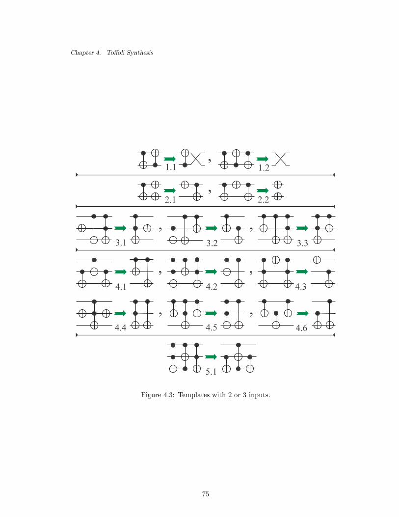
Chapter 4. Toffoli Synthesis
4.6
4.1 4.2
4.5
4.3
4.4
,
,,
,
,,
,
,
3.1
2.1
1.1
3.2
2.2
1.2
3.3
5.1
Figure 4.3: Templates with 2 or 3 inputs.
75

Chapter 4. Toffoli Synthesis
In this section, we give a formal classification of the templates used in [51]. However,
for a better understanding of template classes, we introduce the following notation.
• the left hand side has a sequence of gates that is to be replaced with the sequence
given on the right hand side;
• the controls of the gates are coded by sets Ci, each of which represents a set (which
may be empty) of lines;
• the target sets ti each contain a single line.
All sets are disjoint: Ci ∩ Cj = ∅, Ci ∩ tk = ∅, tl ∩ tk = ∅ ∀i, j, k, l.
Using this notation, a class of templates can be defined as a set of templates which can
be described by one formula. A first attempt to classify the templates results in the
classes listed below:
Class 1. This class unites and generalizes the templates 2.2, 4.1-4.3 (Figure 4.3) into
a class (Figure 4.4) with the formula:
TOF (C1 + C2 + t2, t1) TOF (C1 + C3, t2) TOF (C1 + C2 + t2, t1)
= TOF (C1 + C3, t2) TOF (C1 + C2 + C3, t1) (4.1)
Class 2. This class consists of templates 4.4-4.6 (Figure 4.3) and their generalizations.
The class is illustrated in Figure 4.4 and can be written as the following formula:
TOF (C1 + C2, t2) TOF (C1 + C3 + t2, t1) TOF (C1 + C2, t2)
= TOF (C1 + C3 + t2, t1) TOF (C1 + C2 + C3, t1) (4.2)
76

Chapter 4. Toffoli Synthesis
Class 3. This class (Figure 4.4) includes templates 2.1, 3.1-3.3 (Figure 4.3) and can be
described by the formula:
TOF (C1 + C2 + t2, t1) TOF (C1 + C2 + C3, t1) TOF (C1 + C3, t2)
= TOF (C1 + C3, t2) TOF (C1 + C2 + t2, t1) (4.3)
,CCtt
1
2
3
1
2
,
Class 1.
C
Class 2. Class 3.
CCtt
1
2
3
1
2
C
Figure 4.4: Toffoli templates.
Template 5.1 can be generalized, but this generalization is not considered here since
template 5.1 does not decrease the number of gates in a network. However, the use of a
generalization of this template may be beneficial since it introduces smaller gates that
can be used by other templates. Even if they are not used, it is beneficial to have gates
with fewer controls, since for some technologies their costs are lower. For instance, in
quantum technology the cost of a Toffoli gate is 5 times higher than that of a CNOT
gate. As the number of controls of the Toffoli gate grows, the relation between the costs
of generalized Toffoli and CNOT gates grows quadratically if no additional garbage is
allowed and linearly if additional garbage is allowed [4].
The correctness of formulas (4.1)-(4.3) is easily proven. A more interesting question is
whether the set of these three classes of templates together with the two rules (moving
rule, deletion rule) is a complete set of simplification rules for a sequence of three
generalized Toffoli gates over n lines. To check this, we wrote and ran a program which
77

Chapter 4. Toffoli Synthesis
exhaustively searches all sequences of three gates built on four lines to check whether
the sequence can be reduced by means of templates from the three classes and the two
rules. This program found no new templates. Thus, we conclude that the three classes
together with moving and deletion rules form the complete simplification tool for any
Toffoli network with up to three gates.
4.2.1 Unification of Class 1 and Class 2 Templates
Classes 1 and 2, as illustrated in Fig. 4.4, look similar. This similarity results in the
following description of the two classes as a single class:
• the first part of the template has 3 gates of the form ABA, i.e. the first and the
third gates are the same;
• if the following algorithm produces a valid network, the template exists, otherwise
it does not (correctness can be easily proven):
– Take the second gate and put it first in the second part of the template.
– On each line, there may be a logical AND connection (•), an EXOR (⊕), or
no connection with the vertical line (denoted ¤). We build the second gate
of the right hand side of the template by taking values from Table 4.3 using
the symbols on that line from A and B (since the table is symmetric, there
is no need to specify which argument is A and which is B).
– If the symbol E occurs during the building process, the template cannot be
built. It is easy to see why, since if all ⊕ are on the same line the moving
rule is applicable; the network can be changed to the form AAB, after which
an application of the deletion rule transforms the network to the form B.
78

Chapter 4. Toffoli Synthesis
¤ • ⊕
¤ ¤ • ⊕
• • • ¤
⊕ ⊕ ¤ E
Table 4.3: Second gate building process
– In other cases, for TOF(t1 + t2, t3) TOF(t1 + t3, t2) TOF(t1 + t2, t3) for ex-
ample, the algorithm produces a logical AND on the first line and nothing at
all on the other lines. This makes no sense. That is, no reduction is possible
for this sequence of gates.
4.3 Templates - a New Approach
We further generalize the template tool, but assume the following limitation: the model
gates should necessarily be self-inverses. This limits the generality of a template, but
for the goals of the generalized Toffoli gate synthesis this does not change the essence,
since a generalized Toffoli gate is a self-inverse. Note that Fredkin and Miller gates are
also self-inverses, thus, their addition to the model would be “legal” from the point of
view of the templates.
Although the template description in Section 4.2 is formal and shorter (3 classes and
2 rules in comparison to 14 templates with 2 rules as used before), it can be simplified
even further. For this we need a new understanding of templates.
Let a size m template be a sequence of m gates (a circuit) which realizes the identity
function. Any template of size m must be independent of templates of smaller size, i.e.
79
Chapter 4. Toffoli Synthesis
for a given template size m no application of any set of templates of smaller size can
decrease the number gates. The template G0 G1... Gm−1 (Gi is a reversible gate) can
be applied in two directions:
1. Forward application: A piece of the network that matches the sequence of
gates Gi G(i+1) mod m... G(i+k−1) mod m of the template G0 G1... Gm−1 exactly,
is replaced with the sequence G(i−1) mod m G(i−2) mod m... G(i+k) mod m without
changing the network’s output, where parameter k ∈ N, k ≥ m2 .
2. Backward application: A piece of the network that matches the sequence of
gates Gi G(i−1) mod m... G(i−k+1) mod m exactly, is replaced with the sequence
G(i+1) mod m G(i+2) mod m . . . G(i−k) mod m without changing the network output,
where parameter k ∈ N, k ≥ m2 .
These definitions of template application need a correctness proof that the network
output should not change for each of the listed operations. Correctness can be verified
as follows. Note that a reversible cascade that realizes a function f read in reverse (from
the outputs to the inputs) realizes f−1, its inverse.
First, we prove the correctness of the forward application of a template starting with
element G0. The operation for this case requires the substitution of G0 G1... Gk−1 with
Gm−1 Gm−2... Gk. Since G0 G1... Gm−1 realizes the identity function, Gk Gk+1... Gm−1
realizes the inverse of the function realized by G0 G1... Gk−1. Therefore, if we read in
the reverse order, Gk Gk+1... Gm−1 realizes the inverse of the inverse, i.e. the function
itself. Thus, the function realized by G0 G1... Gk−1 was substituted by itself, which
does not change the output of the network. The correctness of the remaining forward
80
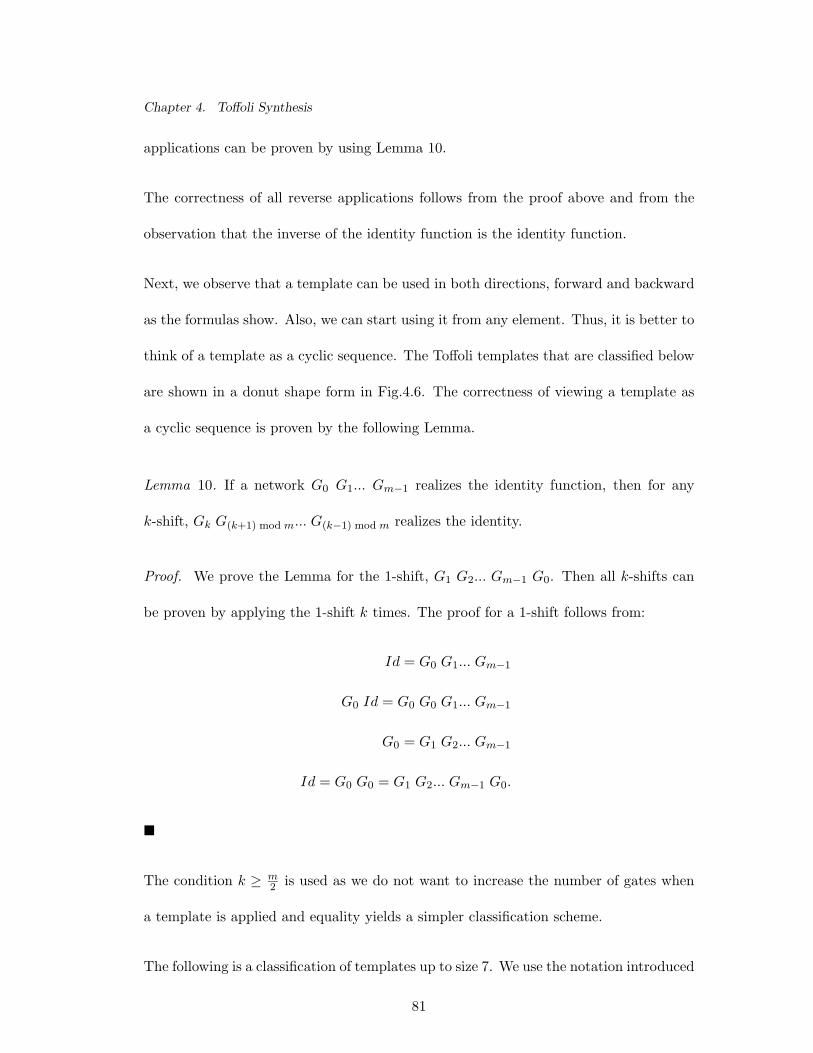
Chapter 4. Toffoli Synthesis
applications can be proven by using Lemma 10.
The correctness of all reverse applications follows from the proof above and from the
observation that the inverse of the identity function is the identity function.
Next, we observe that a template can be used in both directions, forward and backward
as the formulas show. Also, we can start using it from any element. Thus, it is better to
think of a template as a cyclic sequence. The Toffoli templates that are classified below
are shown in a donut shape form in Fig.4.6. The correctness of viewing a template as
a cyclic sequence is proven by the following Lemma.
Lemma 10. If a network G0 G1... Gm−1 realizes the identity function, then for any
k-shift, Gk G(k+1) mod m... G(k−1) mod m realizes the identity.
Proof. We prove the Lemma for the 1-shift, G1 G2... Gm−1 G0. Then all k-shifts can
be proven by applying the 1-shift k times. The proof for a 1-shift follows from:
Id = G0 G1... Gm−1
G0 Id = G0 G0 G1... Gm−1
G0 = G1 G2... Gm−1
Id = G0 G0 = G1 G2... Gm−1 G0.
¥
The condition k ≥ m2 is used as we do not want to increase the number of gates when
a template is applied and equality yields a simpler classification scheme.
The following is a classification of templates up to size 7. We use the notation introduced
81
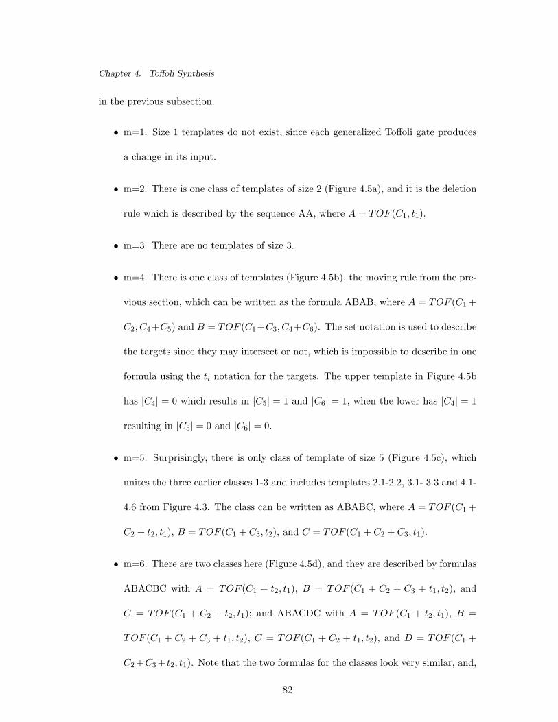
Chapter 4. Toffoli Synthesis
in the previous subsection.
• m=1. Size 1 templates do not exist, since each generalized Toffoli gate produces
a change in its input.
• m=2. There is one class of templates of size 2 (Figure 4.5a), and it is the deletion
rule which is described by the sequence AA, where A = TOF (C1, t1).
• m=3. There are no templates of size 3.
• m=4. There is one class of templates (Figure 4.5b), the moving rule from the pre-
vious section, which can be written as the formula ABAB, where A = TOF (C1 +
C2, C4+C5) and B = TOF (C1+C3, C4+C6). The set notation is used to describe
the targets since they may intersect or not, which is impossible to describe in one
formula using the ti notation for the targets. The upper template in Figure 4.5b
has |C4| = 0 which results in |C5| = 1 and |C6| = 1, when the lower has |C4| = 1
resulting in |C5| = 0 and |C6| = 0.
• m=5. Surprisingly, there is only class of template of size 5 (Figure 4.5c), which
unites the three earlier classes 1-3 and includes templates 2.1-2.2, 3.1- 3.3 and 4.1-
4.6 from Figure 4.3. The class can be written as ABABC, where A = TOF (C1 +
C2 + t2, t1), B = TOF (C1 + C3, t2), and C = TOF (C1 + C2 + C3, t1).
• m=6. There are two classes here (Figure 4.5d), and they are described by formulas
ABACBC with A = TOF (C1 + t2, t1), B = TOF (C1 + C2 + C3 + t1, t2), and
C = TOF (C1 + C2 + t2, t1); and ABACDC with A = TOF (C1 + t2, t1), B =
TOF (C1 + C2 + C3 + t1, t2), C = TOF (C1 + C2 + t1, t2), and D = TOF (C1 +
C2 +C3 + t2, t1). Note that the two formulas for the classes look very similar, and,
82

Chapter 4. Toffoli Synthesis
CCtt
1
2
3
1
2
C
CCt
1
2
3
1
CCCtt
1
2
3
1
2
C
Ct
1
1
CCtt
1
2
3
1
2
C
CCtt
1
2
3
1
2
C
(a)
(b)(c)
(d)
Figure 4.5: All templates for m ≤ 7.
using Fredkin gates, they can be generalized to form one very simple template
FRE(C1 + C2 + C3, t1 + t2) FRE(C1 + C2 + C3, t1 + t2) (where FRE(C, t1 + t2)
is a gate which swaps values of bits t1 and t2 if, and only if, set C has all ones
on its lines), but we do not pursue this here as we are restricting our attention to
generalized Toffoli gates.
• m=7. There are no templates of size 7.
The described templates are also shown as cyclic circuits in Fig.4.6.
To verify the correctness of the above classification, we must show that no template of
larger size can be reduced to a template of smaller size.
• – The size 4 template is independent of the size 2 template, since no adjacent
gates are equal.
• – The size 5 template is independent of the size 2 template, since no adjacent
83
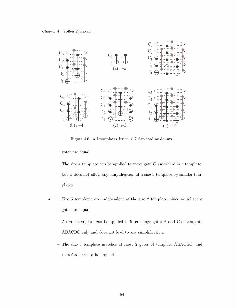
Chapter 4. Toffoli Synthesis
C1t1
CCtt
1
2
3
1
2
C
CC1
2
3C
t1
CC1
2
3C
t1
t2(a) n=2.
(b) n=4. (c) n=5.
CCtt
1
2
3
1
2
C
CCtt
1
2
3
1
2
C
(d) n=6.
Figure 4.6: All templates for m ≤ 7 depicted as donuts.
gates are equal.
– The size 4 template can be applied to move gate C anywhere in a template,
but it does not allow any simplification of a size 5 template by smaller tem-
plates.
• – Size 6 templates are independent of the size 2 template, since no adjacent
gates are equal.
– A size 4 template can be applied to interchange gates A and C of template
ABACBC only and does not lead to any simplification.
– The size 5 template matches at most 2 gates of template ABACBC, and
therefore can not be applied.
84
Chapter 4. Toffoli Synthesis
4.3.1 Completeness
First of all, we wrote a program which builds all the 4-input 4-output circuits of size 7
that realize the identity function and tries to apply the templates. The program result
shows that the set of our 5 templates (AA, ABAB, ABABC, ABACBC, ABACDC) is
the complete set of templates of size 7 or less for 4 inputs and less.
The mathematical proof of completeness of this set for any number of inputs is harder.
For templates of size 2 it can be done by hand, since there are few choices to consider.
For templates of size 4 and 5 the following lemmas are useful.
Lemma 11. A size m template has at most bm2 c different lines with EXOR signs.
Proof. Proof by contradiction. Suppose there are bn2 c + 1 or more lines which contain
an EXOR sign. Then, by the pigeonhole principle, there will be one line with a single
EXOR sign only. Cut the cycle so that the gate with this EXOR, TOF (C, t) comes
first. Now, if we assign 1 to all xj ∈ C, the value of t changes to t as the signal is
propagated in the template. Thus, the template does not realize the identity function,
which contradicts its definition. ¥
Lemma 12. If a size m template has only a single line with EXOR signs, m is even and
all the gates in it can be grouped as pairs of equal gates.
Proof. Proof by contradiction. Suppose not all the gates can be paired or the number
m is odd. Apply passing and duplication deletion rules to delete all the paired gates
from the template. The remaining circuit still realizes the identity since all the applied
operations did not change the circuit output. When we propagate the signal in the
85
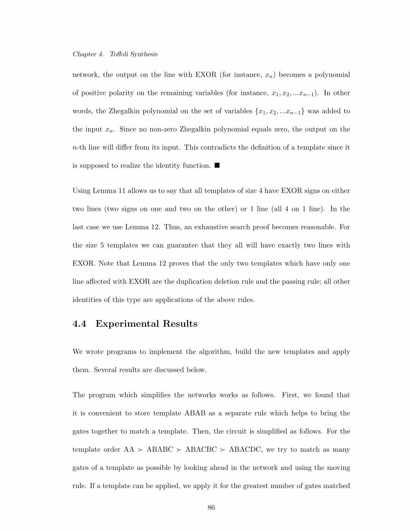
Chapter 4. Toffoli Synthesis
network, the output on the line with EXOR (for instance, xn) becomes a polynomial
of positive polarity on the remaining variables (for instance, x1, x2, ...xn−1). In other
words, the Zhegalkin polynomial on the set of variables {x1, x2, ...xn−1} was added to
the input xn. Since no non-zero Zhegalkin polynomial equals zero, the output on the
n-th line will differ from its input. This contradicts the definition of a template since it
is supposed to realize the identity function. ¥
Using Lemma 11 allows us to say that all templates of size 4 have EXOR signs on either
two lines (two signs on one and two on the other) or 1 line (all 4 on 1 line). In the
last case we use Lemma 12. Thus, an exhaustive search proof becomes reasonable. For
the size 5 templates we can guarantee that they all will have exactly two lines with
EXOR. Note that Lemma 12 proves that the only two templates which have only one
line affected with EXOR are the duplication deletion rule and the passing rule; all other
identities of this type are applications of the above rules.
4.4 Experimental Results
We wrote programs to implement the algorithm, build the new templates and apply
them. Several results are discussed below.
The program which simplifies the networks works as follows. First, we found that
it is convenient to store template ABAB as a separate rule which helps to bring the
gates together to match a template. Then, the circuit is simplified as follows. For the
template order AA Â ABABC Â ABACBC Â ABACDC, we try to match as many
gates of a template as possible by looking ahead in the network and using the moving
rule. If a template can be applied, we apply it for the greatest number of gates matched
86
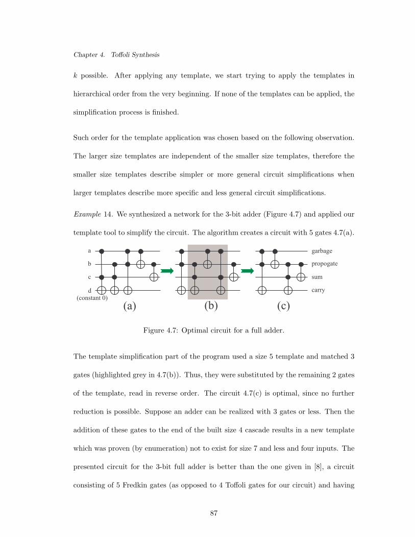
Chapter 4. Toffoli Synthesis
k possible. After applying any template, we start trying to apply the templates in
hierarchical order from the very beginning. If none of the templates can be applied, the
simplification process is finished.
Such order for the template application was chosen based on the following observation.
The larger size templates are independent of the smaller size templates, therefore the
smaller size templates describe simpler or more general circuit simplifications when
larger templates describe more specific and less general circuit simplifications.
Example 14. We synthesized a network for the 3-bit adder (Figure 4.7) and applied our
template tool to simplify the circuit. The algorithm creates a circuit with 5 gates 4.7(a).
a
b
c
d(constant 0)
garbage
carry
sum
propogate
(a) (b) (c)
Figure 4.7: Optimal circuit for a full adder.
The template simplification part of the program used a size 5 template and matched 3
gates (highlighted grey in 4.7(b)). Thus, they were substituted by the remaining 2 gates
of the template, read in reverse order. The circuit 4.7(c) is optimal, since no further
reduction is possible. Suppose an adder can be realized with 3 gates or less. Then the
addition of these gates to the end of the built size 4 cascade results in a new template
which was proven (by enumeration) not to exist for size 7 and less and four inputs. The
presented circuit for the 3-bit full adder is better than the one given in [8], a circuit
consisting of 5 Fredkin gates (as opposed to 4 Toffoli gates for our circuit) and having
87
Chapter 4. Toffoli Synthesis
abcde
f (=0)g(=0)
hhh
0
1
2
abcd
''
''
Figure 4.8: Circuit for rd53.
4 garbage bits (as opposed to 1 garbage bit for our circuit).
Example 15. As a second example we consider the benchmark function rd53. This
function has 5 inputs and 3 outputs. The outputs are the binary encoding of the weight
of the input pattern i.e. the number of 1s in the input pattern. For example, input
00000 yields output 000, input 00100 yields output 001 and input 11111 yields output
101. The maximum output pattern multiplicity is 10, so at least 4 garbage outputs
must be added giving a total of at least 7 outputs. That in turn requires two inputs be
added. Initially the reversible specification given in [50] was used. The garbage outputs
were subsequently modified to remove unnecessary gates. Our algorithm produces a
circuit with 12 gates in 1.84 seconds of CPU time. This is better than the circuit with
14 gates proposed in [54]. It is also better than 13 gates, the result from the previous
chapter.
The larger the set of templates, the more reductions can be done. For instance, if
for some natural number k, k-optimality is defined as the impossibility of simplify-
ing a network with templates of size (2k − 1) and less, then all the templates of size
(n−1)∗2n+1+1 and less form the complete simplification tool for the presented synthesis
88

Chapter 4. Toffoli Synthesis
algorithm.
89
Chapter 5Toffoli-Fredkin Synthesis
5.1 How Useful Are Fredkin Gates?
In this chapter it is shown how to use Fredkin gates in conjunction with Toffoli gates
to produce a smaller network. An important question which arises as soon as the
“Toffoli-Fredkin Synthesis” is proposed is, how useful are Fredkin gates, if they are
useful at all? To answer this question, we wrote a program to calculate the optimal
circuits for all 3-input 3-output reversible functions in terms of the cascades of Toffoli
and Fredkin gates and compared them to previously reported results on the optimal
Toffoli synthesis [74, 75] in Table 5.1. The table shows how many functions of size 3 can
be realized with k = 0, 1, ..., 8 gates in optimal synthesis using NOT, CNOT and Toffoli
gates (NCT column, calculated in [74, 75]), NOT, CNOT, Toffoli, and SWAP gates
(NCTS column, calculated in [74, 75]), and NOT, CNOT, Toffoli, SWAP, and Fredkin
gates (NCTSF column, calculated by us). The “Total:” row of the Table shows how
many different functions in total are presented in the column (to make sure we have all
40320 reversible functions of size 3); the “WA:” row shows the weighted average cost of
a reversible function in terms of the corresponding model. Analysis of this table shows
that the average cost in NCTSF is approximately 0.732 gates lower than the one in
NCT. The maximum cost drops from 8 to 7. The NCTS column looks odd, since the
90
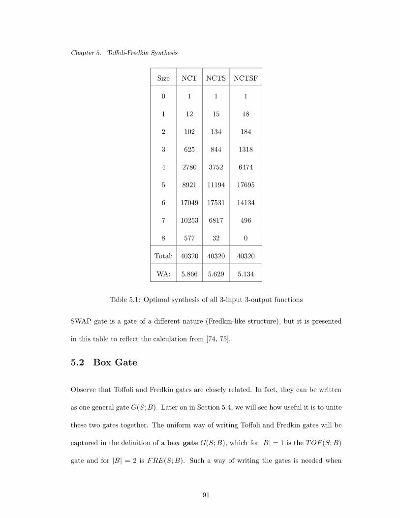
Chapter 5. Toffoli-Fredkin Synthesis
Size NCT NCTS NCTSF
0 1 1 1
1 12 15 18
2 102 134 184
3 625 844 1318
4 2780 3752 6474
5 8921 11194 17695
6 17049 17531 14134
7 10253 6817 496
8 577 32 0
Total: 40320 40320 40320
WA: 5.866 5.629 5.134
Table 5.1: Optimal synthesis of all 3-input 3-output functions
SWAP gate is a gate of a different nature (Fredkin-like structure), but it is presented
in this table to reflect the calculation from [74, 75].
5.2 Box Gate
Observe that Toffoli and Fredkin gates are closely related. In fact, they can be written
as one general gate G(S; B). Later on in Section 5.4, we will see how useful it is to unite
these two gates together. The uniform way of writing Toffoli and Fredkin gates will be
captured in the definition of a box gate G(S; B), which for |B| = 1 is the TOF (S; B)
gate and for |B| = 2 is FRE(S; B). Such a way of writing the gates is needed when
91
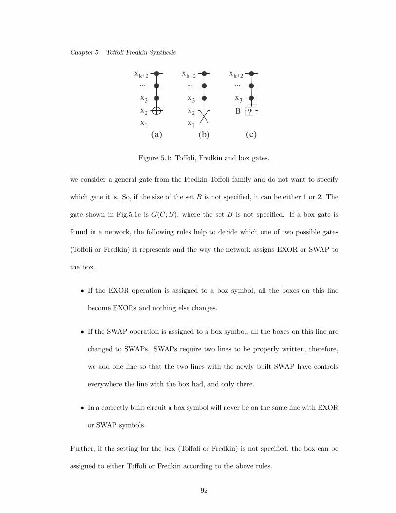
Chapter 5. Toffoli-Fredkin Synthesis
?x1
xx
x
2
3
...k+2
x1
xx
x
2
3
...k+2
x
x
3
...k+2
B
(a) (b) (c)
Figure 5.1: Toffoli, Fredkin and box gates.
we consider a general gate from the Fredkin-Toffoli family and do not want to specify
which gate it is. So, if the size of the set B is not specified, it can be either 1 or 2. The
gate shown in Fig.5.1c is G(C; B), where the set B is not specified. If a box gate is
found in a network, the following rules help to decide which one of two possible gates
(Toffoli or Fredkin) it represents and the way the network assigns EXOR or SWAP to
the box.
• If the EXOR operation is assigned to a box symbol, all the boxes on this line
become EXORs and nothing else changes.
• If the SWAP operation is assigned to a box symbol, all the boxes on this line are
changed to SWAPs. SWAPs require two lines to be properly written, therefore,
we add one line so that the two lines with the newly built SWAP have controls
everywhere the line with the box had, and only there.
• In a correctly built circuit a box symbol will never be on the same line with EXOR
or SWAP symbols.
Further, if the setting for the box (Toffoli or Fredkin) is not specified, the box can be
assigned to either Toffoli or Fredkin according to the above rules.
92
Chapter 5. Toffoli-Fredkin Synthesis
5.2.1 A Note on Similarity of Fredkin And Toffoli Gates
Fredkin gates alone do not form a complete set. Fredkin gates act as controlled SWAPs
which do not change the number of ones in the pattern (like the structure proposed in
[33] and [72], where gates that do not change the number of ones were considered). For
example, the set of all Fredkin gates is not sufficient if the NOT operation is needed.
Will the set of NOT and all Fredkin gates be complete? Given a network of Toffoli gates
is it possible and easy to find a transformation to the NOT-Fredkin network which will
compute the same function (assuming garbage is unlimited)? A positive answer for the
second question implies a positive answer on the first question, since the set of Toffoli
gates is complete (shown constructively in Chapter 4). Here we answer the second
question: given a circuit with Toffoli gates, we can build a circuit with NOT-Fredkin
gates. The construction is as follows.
• Code each Boolean pattern 0 with the pair of Boolean values (1, 0) and each
Boolean pattern 1 with (0, 1).
• Given a Toffoli circuit, split each horizontal line into two. If the splitting line had
no symbol on it, do not put any symbol on the resulting two lines. If the splitting
line had ⊕ sign on it, substitute it with SWAP (which is possible to do after the
line was split). If the line was a control (•), after splitting substitute the first line
with a line of the form NOT-•-NOT, and second line with the control only (•).
• After these transformations are done, the circuit will consist of the NOT and
Fredkin gates only, since all the occurrences of ⊕ were replaced with SWAP.
93

Chapter 5. Toffoli-Fredkin Synthesis
xyz
abc
a
b
c
a
b
c
x
y
z
x
y
z
Figure 5.2: Transformation of a Toffoli circuit to a NOT-Fredkin circuit.
For an example of this circuit transformation, see Fig. 5.2. The NOT-Fredkin circuit
has several nice properties. The Boolean inputs of the function to be calculated are on
even lines, and the corresponding Boolean outputs are even outputs. The second circuit
computes both a function and its negation simultaneously (which in practice may not
be that useful). An interesting observation is that if the inputs and outputs of the
resulting circuit are (naturally) paired and a pair of equal outputs is found, it can be
concluded that at least one of the gates malfunctioned. This property may be useful in
a design-for-testability.
5.3 The algorithm
In this section we consider several Fredkin-Toffoli family synthesis problems: synthesis
of reversible functions, synthesis of multiple output functions, and synthesis of incom-
pletely specified multiple output functions.
The algorithm to be presented is a modified version of the algorithm from Chapter 4.
As usual, the function is specified as a truth table, which contains input patterns on
the left, and output patterns on the right side. All the Boolean patterns are considered
to be arranged in lexicographical order.
94
Chapter 5. Toffoli-Fredkin Synthesis
Start with the basic algorithm which works with completely specified reversible functions
only. The synthesis procedure will start with the empty circuit which realizes the
identity function. At every step of the synthesis algorithm we add a few of gates from
the Fredkin-Toffoli family to the end of the cascade already constructed. Since the
reversible cascade can be built from either end, we have to agree on where to start. For
the basic algorithm it is better to start synthesizing the function from the outputs and
working towards the inputs, so that the cascade is to be read in reverse order.
Basic algorithm.
Step 0. Idea: take the narrowest gates and arrange them in a cascade so that they
bring the first output pattern to the first input pattern.
The first pattern of truth table is the lowest in the order sequence (0, 0, ..., 0), while
the first pattern in the output part is, in general, an unknown pattern (b1, b2, ..., bn).
To bring it to the form (0, 0, ..., 0), we use gates TOF (xi) for every i such that bi 6= 0.
When the first gates are added to the cascade, we update the output part of the table
to see that the pattern (b1, b2, ..., bn) was transformed to the desired form (0, 0, ..., 0).
Step S. Idea: without influencing the patterns of the lower order that were put at their
desired places in the previous steps of the algorithm, use the least number of the nar-
rowest gates to bring the output pattern to the form of the corresponding input pattern.
The input pattern of the table, (a1, a2, ..., an) is the binary representation of the nat-
ural number (S+1). The pattern in the last update of the output part is any pattern
(b1, b2, ..., bn) of higher order. If the order is the same, the patterns are equal, and there
95

Chapter 5. Toffoli-Fredkin Synthesis
is nothing left to do at this step. The order of (b1, b2, ..., bn) cannot be less than the
order of (a1, a2, ..., an) since all such patterns were put to their places in the previous
steps of the algorithm.
For the pattern (b1, b2, ..., bn) to be transformed to (a1, a2, ..., an), note that each ap-
plication of a Toffoli gate is capable of flipping one bit of the pattern (b1, b2, ..., bn),
and each Fredkin gate is capable of permuting a pair of unequal Boolean values. Now,
the problem can be formulated as follows: using the two operations “flip” and “swap”,
bring a Boolean pattern (b1, b2, ..., bn) Â (a1, a2, ..., an) to the form (a1, a2, ..., an) so that
all intermediate Boolean patterns are greater than (a1, a2, ..., an). The controls for the
corresponding gates will be assigned later. The solution is as follows.
• If the number of ones in (b1, b2, ..., bn) is less than the number of ones in (a1, a2, ..., an)
try to apply as many “swaps” as we can and then flip the remaining zero bits to
one. Use “swaps” so that the order of each intermediate pattern (x1, x2, ..., xn) is
less than the order of (a1, a2, ..., an), and define the set of controls as a minimal
subset of unit values of (x1, x2, ..., xn), such that this subset forms a Boolean pat-
tern of an order higher than (a1, a2, ..., an). This can be easily done if “swaps” are
done on the lower end of the pattern first. Note that in this case the initial pat-
tern (b1, b2, ..., bn) was greater than (a1, a2, ..., an), so the most significant binary
digit of (b1, b2, ..., bn) equal to one was greater than the most significant digit of
(a1, a2, ..., an) equal to 1. Thus, this digit will be taken as the control (when a
control is needed) for all corresponding Fredkin and Toffoli gates except the last
Toffoli gate, for which the control will consist of all digits of (a1, a2, ..., an) that
are equal to 1.
96
Chapter 5. Toffoli-Fredkin Synthesis
• If the number of ones in (b1, b2, ..., bn) is equal to the number of ones in (a1, a2, ..., an),
then it is possible to transform one pattern into other using “swap” operation only.
Controls are then found by the procedure described in the above case.
• If the number of ones in (b1, b2, ..., bn) is greater than the number of ones in
(a1, a2, ..., an), then apply “swaps” starting from the end of the pattern (b1, b2, ..., bn)
and then apply necessary Toffoli gates. All the necessary controls can be found
using the procedure from the first case.
Step 2n − 1. When all (2n − 1) previous patterns are in their places, the last patterns
will automatically match.
Motivation. In technology it usually happens that the narrower the gate, the lower its
cost, and thus we try to use the narrowest gates. However, choosing the narrowest gates
at each step may lead to larger initial circuits which might not be simplified enough
by the template tool. Therefore, in the actual implementation of this algorithm we
define which gate to take by choosing the one producing a circuit whose output has the
shortest Hamming distance to the desired input pattern we are attempting to match.
Such a method of choosing a gate has no theory behind it, but we use it because it
makes sense. It also happens that the template simplification tool is sensitive to the
width of the gates, so we prepare the circuit for better template reduction by taking
narrow gates.
Bidirectional modification. The basic algorithm works from the output to input by
adding the gates in one direction starting from the end of desired cascade and ending at
its beginning. What if we were able to understand what happens if during the procedure
97
Chapter 5. Toffoli-Fredkin Synthesis
a gate is added to the beginning of cascade? Then we would be able to construct the
network from the two ends simultaneously by growing the number of gates from the
two sides. The idea of the method stays the same; by applying the gates, we bring the
input and output parts of the truth table to each other by assuring that at each step
of the calculation we put at least one pattern at its place. It makes sense that such
a bidirectional algorithm in average will converge faster. We next take any function
written as a truth table, apply a gate and see what change it makes in the output part
of the truth table.
• Toffoli gate application. Without loss of generality we apply gate TOF (C; xk+1),
C = {x1, x2, ..., xk} with the controls on first k variables and target on the (k +1)
variable (all other generalized Toffoli gates have permuted set of controls and,
maybe, a different target). Then, in the input part of the truth table the patterns
(1, 1, ..., 1, x0k+1, x
0k+2, ..., x
0n) will interchange with patterns (1, 1, ..., 1, x0
k+1, x0k+2, ..., x
0n).
In terms of our understanding, this is the same as permuting the output patterns
in front of the (1, 1, ..., 1, x0k+1, x
0k+2, ..., x
0n) and (1, 1, ..., 1, x0
k+1, x0k+2, ..., x
0n) input
patterns without changing the input part. This procedure is easier to visualize,
since the matched patterns do not get mixed up in the middle of the truth table,
which would make it hard to track a pattern. For the program implementation,
the input part may be changed (from the point of view of the computer this does
not confuse any patterns).
• Fredkin gate application. We apply a Fredkin gate FRE(C; xk+1, xk+2), C =
{x1, x2, ..., xk}. This results in the following change of all patterns in the in-
put part of the table: (1, 1, ..., 1, x0k+1, x
0k+2, x
0k+3, ..., x
0n) is interchanged with
98
Chapter 5. Toffoli-Fredkin Synthesis
(1, 1, ..., 1, x0k+2, x
0k+1, x
0k+3, ..., x
0n). If we want to keep the conventional form of
the input part of the truth table when patterns are arranged lexicographically,
this operation is the same as interchanging the output patterns of the truth table
which stay in front of the input patterns (1, 1, ..., 1, x0k+1, x
0k+2, x
0k+3, ..., x
0n) and
(1, 1, ..., 1, x0k+2, x
0k+1, x
0k+3, ..., x
0n).
The bidirectional algorithm thus has the same number of steps, where at each step it
tries to change the output pattern so that it matches the input pattern by applying the
least number of the narrowest gates assigned at either side of the cascade.
The presented algorithm is an improved version of the algorithm suggested in Chapter
4, since the new algorithm uses the Fredkin gates.
Function 3 17 introduced in Chapter 4 had the cost of 17 when realized as a Toffoli
cascade. Now, it will serve as a good example of how helpful it is to use the Fredkin
gates.
Example 16. We apply the basic method for the 3 17 function, shown in the truth table
in Table 5.2.
• Step 0. The output pattern corresponding to the input pattern (0, 0, 0) is (1, 1, 1).
In order to bring it to the form (0, 0, 0) we use 3 NOTs: TOF (a), TOF (b) and
TOF (c). Not, that this is not a unique way of changing the output pattern to
make it match the input, since, for instance, TOF (b, c; a), TOF (c; b) and TOF (c)
would do the same. Thus, the program realization may branch or use a heuristic to
choose the gates, although, for this case the sequence of 3 NOTs defines the unique
way of transforming the output pattern so that the least number of controls is
99
Chapter 5. Toffoli-Fredkin Synthesis
used. An update in the table (Tab.5.2 S1) illustrates that the new output pattern
matches the new input pattern.
• Step 1. For input pattern (0, 0, 1) we have the output pattern (1, 1, 0). In order
to bring the last to the form of input, we swap bits b and c by FRE(b, c) and
then use TOF (c, a) to bring the “swapped” pattern (1, 0, 1) to the form (0, 0, 1).
Neither of the used gates changes anything in the order less than (0, 0, 1). Also
note that this is not a unique way of changing the output pattern to match the
input pattern even for the smallest set of controls: FRE(a, c), TOF (c; b) would
do the same job. Again, this is a place for a program to make a good choice.
• Step 2. The next input pattern, (0, 1, 0), does not match the corresponding output
pattern, (1, 1, 1) (Tab.5.2 S2). We apply the gates TOF (b; c), TOF (b; a) to make
the match.
• Step 3. We apply TOF (a; c) and FRE(c; a, b) to match the output pattern (1, 0, 0)
of Tab.5.2 S2 to the desired input pattern (0, 1, 1).
• Step 4. We use TOF (a; c) and TOF (a; b) to bring (1, 1, 1) (Tab.5.2 S4) to the
form (1, 0, 0).
• Step 5. Finally, we use the FRE(a; b, c) to transform (1, 1, 0) from Tab.5.2 S5 to
(1, 0, 1).
• Steps 6,7 are empty since the output completely matches the input at the previous
step (Tab.5.2 S6).
The resulting circuit has 12 gates, as opposed to 17 for the basic approach in a model
when only Toffoli gates are used. The circuit is illustrated in Fig. 5.3(a).
100
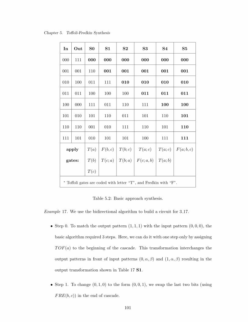
Chapter 5. Toffoli-Fredkin Synthesis
In Out S0 S1 S2 S3 S4 S5
000 111 000 000 000 000 000 000
001 001 110 001 001 001 001 001
010 100 011 111 010 010 010 010
011 011 100 100 100 011 011 011
100 000 111 011 110 111 100 100
101 010 101 110 011 101 110 101
110 110 001 010 111 110 101 110
111 101 010 101 101 100 111 111
apply T (a) F (b, c) T (b; c) T (a; c) T (a; c) F (a; b, c)
gates: T (b) T (c; a) T (b; a) F (c; a, b) T (a; b)
T (c)
∗ Toffoli gates are coded with letter “T”, and Fredkin with “F”.
Table 5.2: Basic approach synthesis.
Example 17. We use the bidirectional algorithm to build a circuit for 3 17.
• Step 0. To match the output pattern (1, 1, 1) with the input pattern (0, 0, 0), the
basic algorithm required 3 steps. Here, we can do it with one step only by assigning
TOF (a) to the beginning of the cascade. This transformation interchanges the
output patterns in front of input patterns (0, α, β) and (1, α, β) resulting in the
output transformation shown in Table 17 S1.
• Step 1. To change (0, 1, 0) to the form (0, 0, 1), we swap the last two bits (using
FRE(b, c)) in the end of cascade.
101
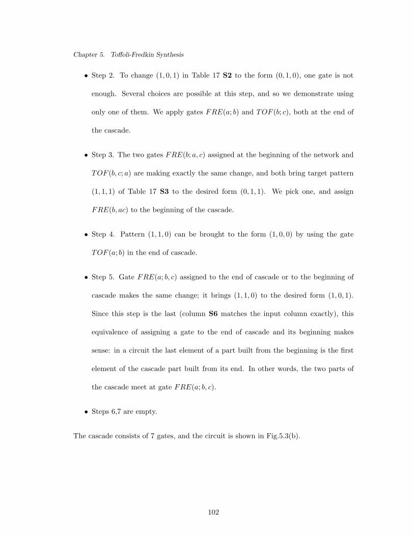
Chapter 5. Toffoli-Fredkin Synthesis
• Step 2. To change (1, 0, 1) in Table 17 S2 to the form (0, 1, 0), one gate is not
enough. Several choices are possible at this step, and so we demonstrate using
only one of them. We apply gates FRE(a; b) and TOF (b; c), both at the end of
the cascade.
• Step 3. The two gates FRE(b; a, c) assigned at the beginning of the network and
TOF (b, c; a) are making exactly the same change, and both bring target pattern
(1, 1, 1) of Table 17 S3 to the desired form (0, 1, 1). We pick one, and assign
FRE(b, ac) to the beginning of the cascade.
• Step 4. Pattern (1, 1, 0) can be brought to the form (1, 0, 0) by using the gate
TOF (a; b) in the end of cascade.
• Step 5. Gate FRE(a; b, c) assigned to the end of cascade or to the beginning of
cascade makes the same change; it brings (1, 1, 0) to the desired form (1, 0, 1).
Since this step is the last (column S6 matches the input column exactly), this
equivalence of assigning a gate to the end of cascade and its beginning makes
sense: in a circuit the last element of a part built from the beginning is the first
element of the cascade part built from its end. In other words, the two parts of
the cascade meet at gate FRE(a; b, c).
• Steps 6,7 are empty.
The cascade consists of 7 gates, and the circuit is shown in Fig.5.3(b).
102

Chapter 5. Toffoli-Fredkin Synthesis
In Out S0 S1 S2 S3 S4 S5
000 111 000 000 000 000 000 000
001 001 010 001 001 001 001 001
010 100 110 101 010 010 010 010
011 011 101 110 111 011 011 011
100 000 111 111 110 110 100 100
101 010 001 010 100 100 110 101
110 110 100 100 011 111 101 110
111 101 011 011 101 101 111 111
apply →T (a) ←F (b, c) ←F (a, b) →F (b; a, c) ←T (a; b) →F (a; b, c)
gates: ←T (b; c)
∗ Toffoli gates are coded with letter “T”, and Fredkin with “F”.
Table 5.3: Bidirectional approach synthesis.
5.3.1 Handling permutations
By permuting the output patterns, one can achieve a reduced cost for the resulting
circuit. The output pattern permutation is the result of applying a certain number
of SWAPs to the end of the cascade, thus, to achieve a fair comparison of the costs of
circuits built with and without output permutations, the corresponding number of swaps
should be added to the cost of a circuit built with output permutations. Currently, we
have no rule for choosing the best permutation, and so for small functions we try all
possibilities.
103
Chapter 5. Toffoli-Fredkin Synthesis
abc
abc
(a) (b)
Figure 5.3: Circuits.
5.3.2 Multiple output and incompletely specified functions
For multiple output functions there are two ways of creating a reversible circuit. First,
make the function reversible using Theorem 1, and then run the bidirectional algorithm.
Second, find the minimum amount of garbage and add garbage outputs without speci-
fying them. Then, take this incompletely specified reversible function and start running
the forward method by specifying the output patterns as soon as we want to assign a
gate in a way which produces the minimum cost circuit possible. Actual procedures of
assigning the output patterns so that it minimizes the network cost are currently under
investigation.
The following a rough idea on how the computation can be performed; the actual
implementation is currently under investigation and is not part of the presented thesis.
5.4 Template simplification tool
We keep the same definition of a template as the one introduced in Section 4.3. Namely,
let a size m template be a sequence of m gates (a circuit) which realizes the identity
function.
The set of Toffoli and Fredkin gates is more complicated than the set of Toffoli gates
only, therefore we redefine the notion of a class of templates.
104
Chapter 5. Toffoli-Fredkin Synthesis
Definition 11. A class of templates of size m is a circuit G(S1; B1) G(S2; B2)...
G(Sm; Bm) with the set of logical conditions on sets S1, B1, S2, B2, ..., Sm, Bm. When a
class is mentioned, it may be written as Gi1 Gi2 ... Gim , where ik = ij iff Sk = Sj and
Bk = Bj .
This approach to defining a class is useful for its short classification, but it is difficult
to visualize. Thus, we introduce the following notation.
Definition 12. A class can be written as a set of disjoint formulas G1(S1, B1) G2(S2, B2)
...Gm(Sm, Bm), where:
• according to the number of elements in Bi, Gi is written as TOF (|Bi| = 1) or
FRE(|Bi| = 2);
• Si is written as a union of sets (Cik) and single variables (tij ) each of which is a
set of one variable only: Si = Ci1 + Ci2 + ... + Cik + ti1 + ti2 + ... + tij ;
• if |Bi| = 1, it is written as single variable, tj ; if |Bi| = 1 it is written as union
tj + tk;
• all the sets are disjoint: Ci ∩ Cj = ∅, Cj ∩ tk = ∅, tk ∩ tl = ∅.
In order to classify templates, we need to discuss the box notation in more detail. If
a box is found in a network, there are certain rules of changing the network when the
operation EXOR or SWAP is assigned to the box.
• If the assignment was EXOR, then the box is substituted with the EXOR symbol.
If the line with the box assigned EXOR contains other box symbols, they are all
105
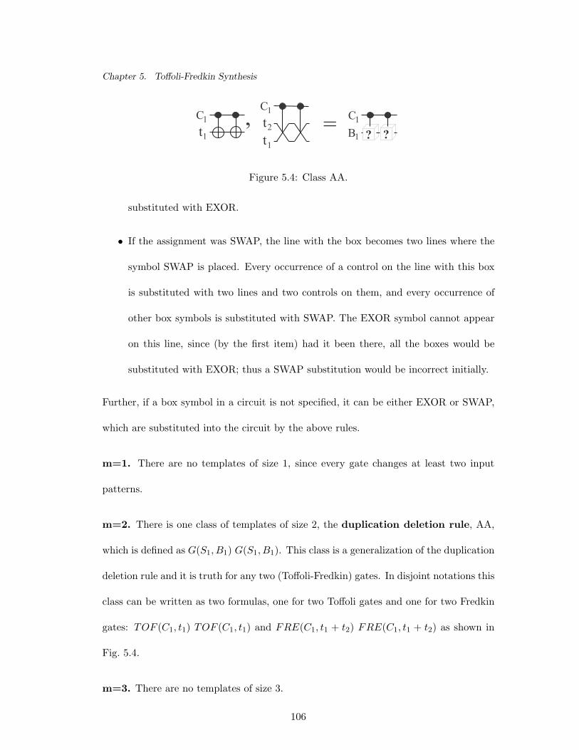
Chapter 5. Toffoli-Fredkin Synthesis
Ct
Ctt1
21
1
1 ?
CB
1
1 ?, =
Figure 5.4: Class AA.
substituted with EXOR.
• If the assignment was SWAP, the line with the box becomes two lines where the
symbol SWAP is placed. Every occurrence of a control on the line with this box
is substituted with two lines and two controls on them, and every occurrence of
other box symbols is substituted with SWAP. The EXOR symbol cannot appear
on this line, since (by the first item) had it been there, all the boxes would be
substituted with EXOR; thus a SWAP substitution would be incorrect initially.
Further, if a box symbol in a circuit is not specified, it can be either EXOR or SWAP,
which are substituted into the circuit by the above rules.
m=1. There are no templates of size 1, since every gate changes at least two input
patterns.
m=2. There is one class of templates of size 2, the duplication deletion rule, AA,
which is defined as G(S1, B1) G(S1, B1). This class is a generalization of the duplication
deletion rule and it is truth for any two (Toffoli-Fredkin) gates. In disjoint notations this
class can be written as two formulas, one for two Toffoli gates and one for two Fredkin
gates: TOF (C1, t1) TOF (C1, t1) and FRE(C1, t1 + t2) FRE(C1, t1 + t2) as shown in
Fig. 5.4.
m=3. There are no templates of size 3.
106
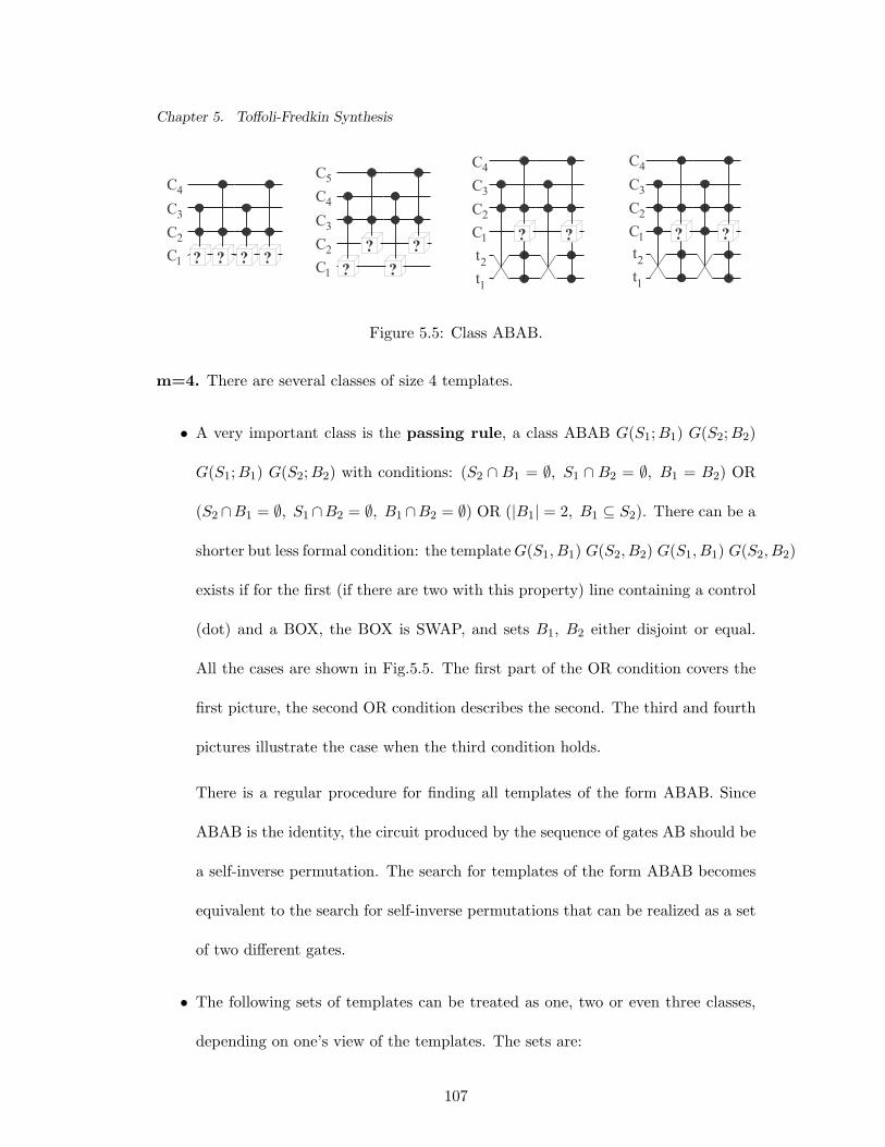
Chapter 5. Toffoli-Fredkin Synthesis
?C1 ?
C2
C3
C4
? ??C1
?C2
C3
C4
??
C5
C1
C2
C3
1
2tt
C1
C2
C3
1
2tt
? ?
C4
? ?
C4
Figure 5.5: Class ABAB.
m=4. There are several classes of size 4 templates.
• A very important class is the passing rule, a class ABAB G(S1; B1) G(S2; B2)
G(S1; B1) G(S2; B2) with conditions: (S2 ∩ B1 = ∅, S1 ∩ B2 = ∅, B1 = B2) OR
(S2 ∩B1 = ∅, S1 ∩B2 = ∅, B1 ∩B2 = ∅) OR (|B1| = 2, B1 ⊆ S2). There can be a
shorter but less formal condition: the template G(S1, B1) G(S2, B2) G(S1, B1) G(S2, B2)
exists if for the first (if there are two with this property) line containing a control
(dot) and a BOX, the BOX is SWAP, and sets B1, B2 either disjoint or equal.
All the cases are shown in Fig.5.5. The first part of the OR condition covers the
first picture, the second OR condition describes the second. The third and fourth
pictures illustrate the case when the third condition holds.
There is a regular procedure for finding all templates of the form ABAB. Since
ABAB is the identity, the circuit produced by the sequence of gates AB should be
a self-inverse permutation. The search for templates of the form ABAB becomes
equivalent to the search for self-inverse permutations that can be realized as a set
of two different gates.
• The following sets of templates can be treated as one, two or even three classes,
depending on one’s view of the templates. The sets are:
107
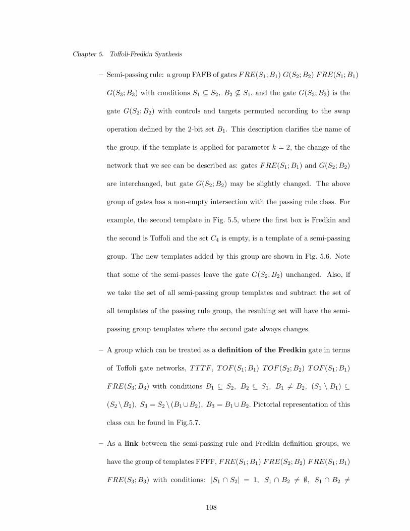
Chapter 5. Toffoli-Fredkin Synthesis
– Semi-passing rule: a group FAFB of gates FRE(S1; B1) G(S2; B2) FRE(S1; B1)
G(S3; B3) with conditions S1 ⊆ S2, B2 6⊆ S1, and the gate G(S3; B3) is the
gate G(S2; B2) with controls and targets permuted according to the swap
operation defined by the 2-bit set B1. This description clarifies the name of
the group; if the template is applied for parameter k = 2, the change of the
network that we see can be described as: gates FRE(S1; B1) and G(S2; B2)
are interchanged, but gate G(S2; B2) may be slightly changed. The above
group of gates has a non-empty intersection with the passing rule class. For
example, the second template in Fig. 5.5, where the first box is Fredkin and
the second is Toffoli and the set C4 is empty, is a template of a semi-passing
group. The new templates added by this group are shown in Fig. 5.6. Note
that some of the semi-passes leave the gate G(S2; B2) unchanged. Also, if
we take the set of all semi-passing group templates and subtract the set of
all templates of the passing rule group, the resulting set will have the semi-
passing group templates where the second gate always changes.
– A group which can be treated as a definition of the Fredkin gate in terms
of Toffoli gate networks, TTTF , TOF (S1; B1) TOF (S2; B2) TOF (S1; B1)
FRE(S3; B3) with conditions B1 ⊆ S2, B2 ⊆ S1, B1 6= B2, (S1 \ B1) ⊆
(S2 \B2), S3 = S2 \ (B1∪B2), B3 = B1∪B2. Pictorial representation of this
class can be found in Fig.5.7.
– As a link between the semi-passing rule and Fredkin definition groups, we
have the group of templates FFFF, FRE(S1; B1) FRE(S2; B2) FRE(S1; B1)
FRE(S3; B3) with conditions: |S1 ∩ S2| = 1, S1 ∩ B2 6= ∅, S1 ∩ B2 6=
108
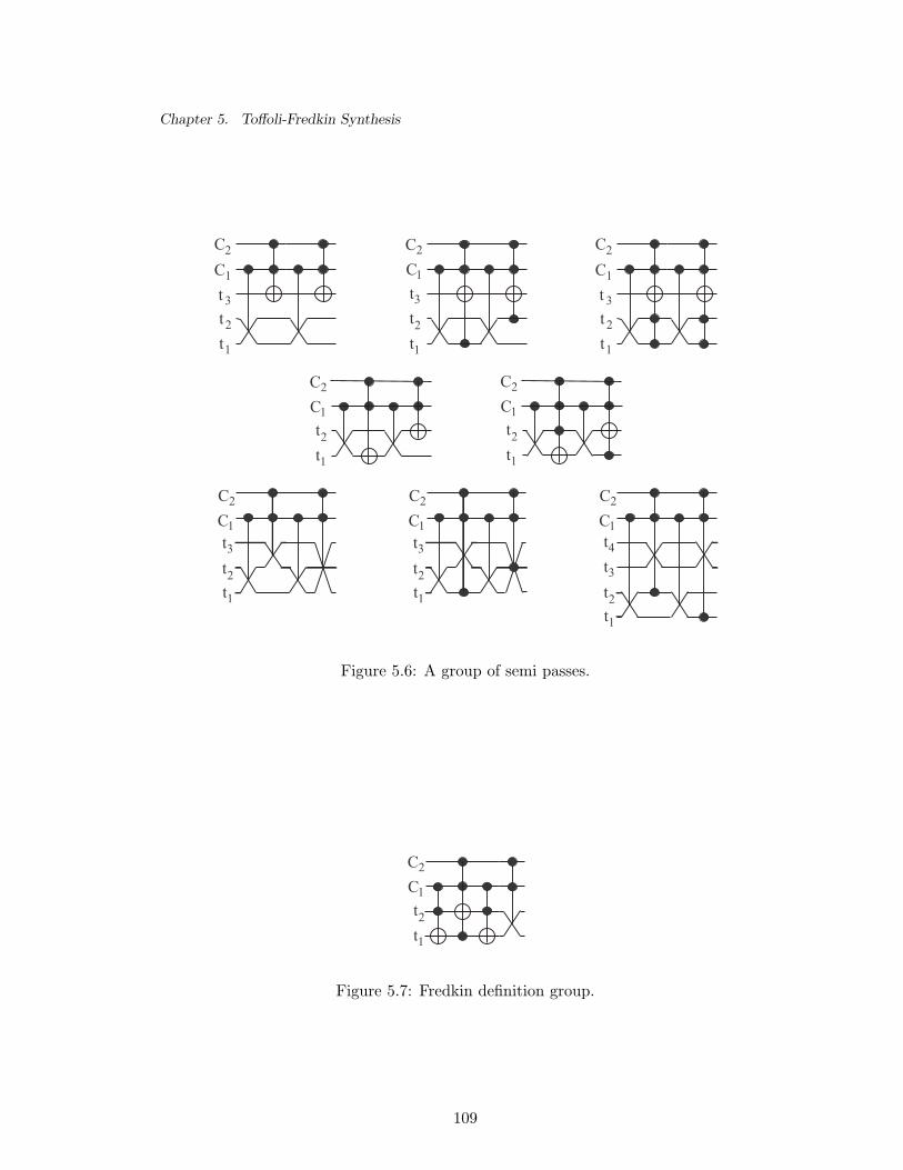
Chapter 5. Toffoli-Fredkin Synthesis
t
1
C1
C2
tt
2
3 t
1
C1
C2
tt
2
3
CCtt
1
2
1
2
t
CC
tt
1
2
3
1
2
CCtt
1
2
1
2
t
CC
tt
1
2
3
1
2
t
CC
tt
1
2
3
1
2
CC1
2
ttt
3
1
2
t4
Figure 5.6: A group of semi passes.
CCtt
1
2
1
2
Figure 5.7: Fredkin definition group.
109
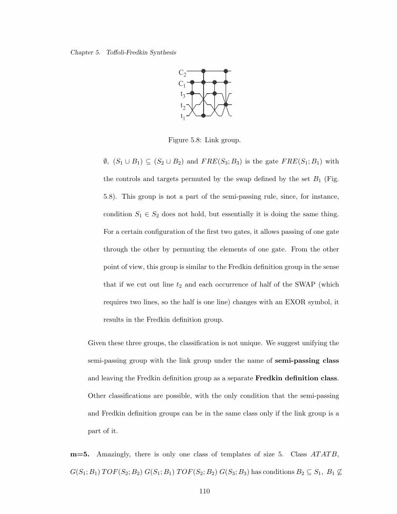
Chapter 5. Toffoli-Fredkin Synthesis
t
CC
tt
1
2
3
1
2
Figure 5.8: Link group.
∅, (S1 ∪ B1) ⊆ (S2 ∪ B2) and FRE(S3; B3) is the gate FRE(S1; B1) with
the controls and targets permuted by the swap defined by the set B1 (Fig.
5.8). This group is not a part of the semi-passing rule, since, for instance,
condition S1 ∈ S2 does not hold, but essentially it is doing the same thing.
For a certain configuration of the first two gates, it allows passing of one gate
through the other by permuting the elements of one gate. From the other
point of view, this group is similar to the Fredkin definition group in the sense
that if we cut out line t2 and each occurrence of half of the SWAP (which
requires two lines, so the half is one line) changes with an EXOR symbol, it
results in the Fredkin definition group.
Given these three groups, the classification is not unique. We suggest unifying the
semi-passing group with the link group under the name of semi-passing class
and leaving the Fredkin definition group as a separate Fredkin definition class.
Other classifications are possible, with the only condition that the semi-passing
and Fredkin definition groups can be in the same class only if the link group is a
part of it.
m=5. Amazingly, there is only one class of templates of size 5. Class ATATB,
G(S1; B1) TOF (S2; B2) G(S1; B1) TOF (S2; B2) G(S3; B3) has conditions B2 ⊆ S1, B1 6⊆
110
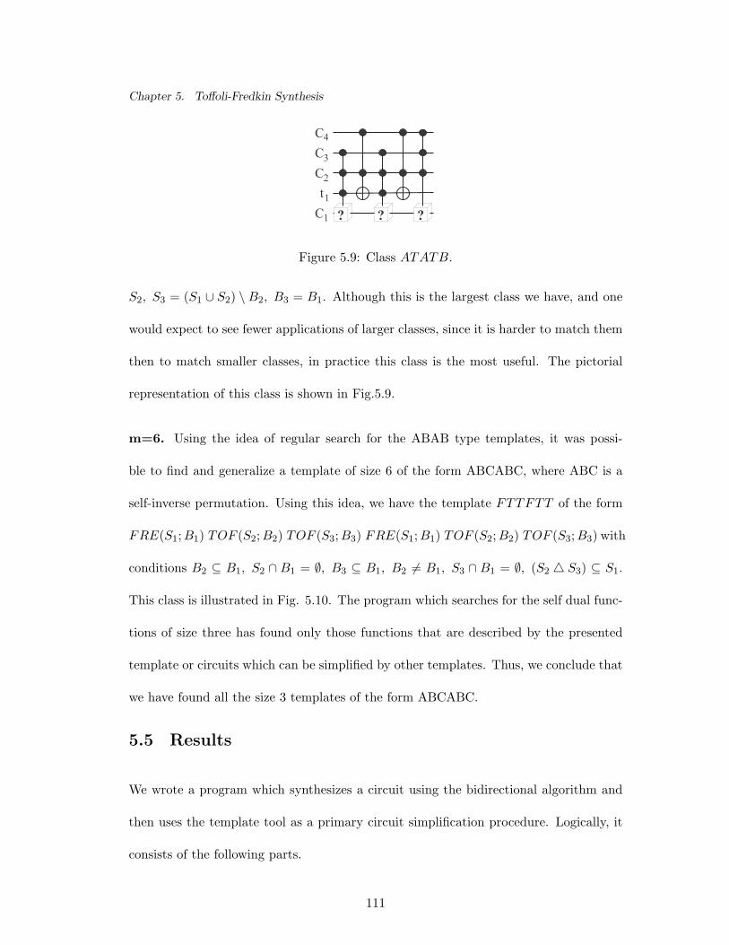
Chapter 5. Toffoli-Fredkin Synthesis
?
C2
C3
? ?
tC1
1
C4
Figure 5.9: Class ATATB.
S2, S3 = (S1 ∪ S2) \ B2, B3 = B1. Although this is the largest class we have, and one
would expect to see fewer applications of larger classes, since it is harder to match them
then to match smaller classes, in practice this class is the most useful. The pictorial
representation of this class is shown in Fig.5.9.
m=6. Using the idea of regular search for the ABAB type templates, it was possi-
ble to find and generalize a template of size 6 of the form ABCABC, where ABC is a
self-inverse permutation. Using this idea, we have the template FTTFTT of the form
FRE(S1; B1) TOF (S2; B2) TOF (S3; B3) FRE(S1; B1) TOF (S2; B2) TOF (S3; B3) with
conditions B2 ⊆ B1, S2 ∩ B1 = ∅, B3 ⊆ B1, B2 6= B1, S3 ∩ B1 = ∅, (S2 4 S3) ⊆ S1.
This class is illustrated in Fig. 5.10. The program which searches for the self dual func-
tions of size three has found only those functions that are described by the presented
template or circuits which can be simplified by other templates. Thus, we conclude that
we have found all the size 3 templates of the form ABCABC.
5.5 Results
We wrote a program which synthesizes a circuit using the bidirectional algorithm and
then uses the template tool as a primary circuit simplification procedure. Logically, it
consists of the following parts.
111
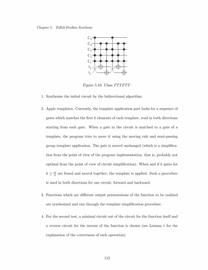
Chapter 5. Toffoli-Fredkin Synthesis
C1
C2
C3
1
2tt
C4
C5
Figure 5.10: Class FTTFTT .
1. Synthesize the initial circuit by the bidirectional algorithm.
2. Apply templates. Currently, the template application part looks for a sequence of
gates which matches the first k elements of each template, read in both directions
starting from each gate. When a gate in the circuit is matched to a gate of a
template, the program tries to move it using the moving rule and semi-passing
group template application. The gate is moved unchanged (which is a simplifica-
tion from the point of view of the program implementation, that is, probably not
optimal from the point of view of circuit simplification). When and if k gates for
k ≥ m2 are found and moved together, the template is applied. Such a procedure
is used in both directions for one circuit, forward and backward.
3. Functions which are different output permutations of the function to be realized
are synthesized and run through the template simplification procedure.
4. For the second test, a minimal circuit out of the circuit for the function itself and
a reverse circuit for the inverse of the function is chosen (see Lemma 1 for the
explanation of the correctness of such operation).
112
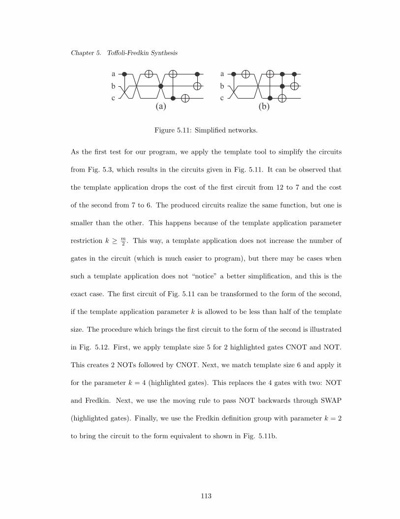
Chapter 5. Toffoli-Fredkin Synthesis
abc
abc
(a) (b)
Figure 5.11: Simplified networks.
As the first test for our program, we apply the template tool to simplify the circuits
from Fig. 5.3, which results in the circuits given in Fig. 5.11. It can be observed that
the template application drops the cost of the first circuit from 12 to 7 and the cost
of the second from 7 to 6. The produced circuits realize the same function, but one is
smaller than the other. This happens because of the template application parameter
restriction k ≥ m2 . This way, a template application does not increase the number of
gates in the circuit (which is much easier to program), but there may be cases when
such a template application does not “notice” a better simplification, and this is the
exact case. The first circuit of Fig. 5.11 can be transformed to the form of the second,
if the template application parameter k is allowed to be less than half of the template
size. The procedure which brings the first circuit to the form of the second is illustrated
in Fig. 5.12. First, we apply template size 5 for 2 highlighted gates CNOT and NOT.
This creates 2 NOTs followed by CNOT. Next, we match template size 6 and apply it
for the parameter k = 4 (highlighted gates). This replaces the 4 gates with two: NOT
and Fredkin. Next, we use the moving rule to pass NOT backwards through SWAP
(highlighted gates). Finally, we use the Fredkin definition group with parameter k = 2
to bring the circuit to the form equivalent to shown in Fig. 5.11b.
113
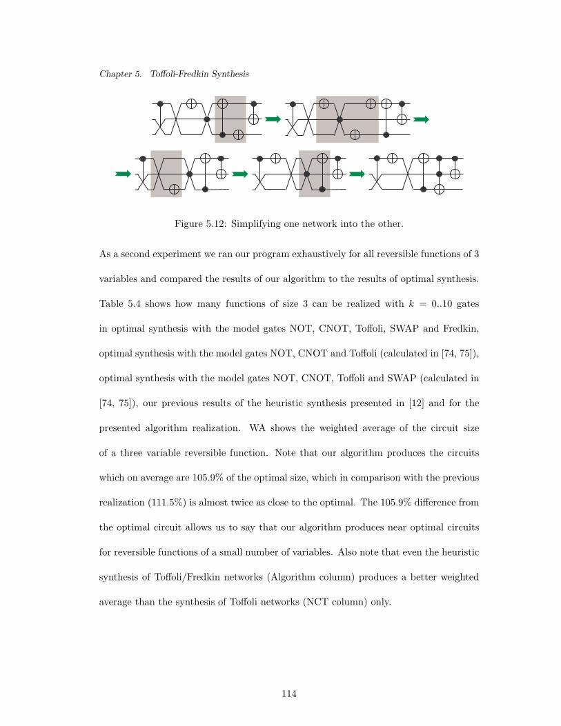
Chapter 5. Toffoli-Fredkin Synthesis
Figure 5.12: Simplifying one network into the other.
As a second experiment we ran our program exhaustively for all reversible functions of 3
variables and compared the results of our algorithm to the results of optimal synthesis.
Table 5.4 shows how many functions of size 3 can be realized with k = 0..10 gates
in optimal synthesis with the model gates NOT, CNOT, Toffoli, SWAP and Fredkin,
optimal synthesis with the model gates NOT, CNOT and Toffoli (calculated in [74, 75]),
optimal synthesis with the model gates NOT, CNOT, Toffoli and SWAP (calculated in
[74, 75]), our previous results of the heuristic synthesis presented in [12] and for the
presented algorithm realization. WA shows the weighted average of the circuit size
of a three variable reversible function. Note that our algorithm produces the circuits
which on average are 105.9% of the optimal size, which in comparison with the previous
realization (111.5%) is almost twice as close to the optimal. The 105.9% difference from
the optimal circuit allows us to say that our algorithm produces near optimal circuits
for reversible functions of a small number of variables. Also note that even the heuristic
synthesis of Toffoli/Fredkin networks (Algorithm column) produces a better weighted
average than the synthesis of Toffoli networks (NCT column) only.
114
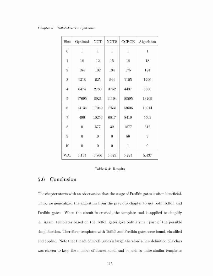
Chapter 5. Toffoli-Fredkin Synthesis
Size Optimal NCT NCTS CCECE Algorithm
0 1 1 1 1 1
1 18 12 15 18 18
2 184 102 134 175 184
3 1318 625 844 1105 1290
4 6474 2780 3752 4437 5680
5 17695 8921 11194 10595 13209
6 14134 17049 17531 13606 13914
7 496 10253 6817 8419 5503
8 0 577 32 1877 512
9 0 0 0 86 9
10 0 0 0 1 0
WA: 5.134 5.866 5.629 5.724 5.437
Table 5.4: Results
5.6 Conclusion
The chapter starts with an observation that the usage of Fredkin gates is often beneficial.
Thus, we generalized the algorithm from the previous chapter to use both Toffoli and
Fredkin gates. When the circuit is created, the template tool is applied to simplify
it. Again, templates based on the Toffoli gates give only a small part of the possible
simplification. Therefore, templates with Toffoli and Fredkin gates were found, classified
and applied. Note that the set of model gates is large, therefore a new definition of a class
was chosen to keep the number of classes small and be able to unite similar templates
115
Chapter 5. Toffoli-Fredkin Synthesis
into one class. The results that we obtain for the heuristic synthesis of Toffoli-Fredkin
family are competitive with other methods. They are only 105.9% higher than the
optimal results for Toffoli-Fredkin synthesis and better than the optimal results for
Toffoli synthesis (for number of variables n = 3).
116
Chapter 6Asymptotically Optimal RegularSynthesis
The synthesis algorithm introduced in Chapter 3 was later transformed into an algorithm
to synthesize Toffoli networks in Chapter 4, and modified one more time in Chapter 5
to use Fredkin gates. It is hard to recognize the old algorithm in it, but historically
the Toffoli synthesis algorithm arrived as a modification of the theoretical synthesis
algorithm for RCMG model. Further modification of this algorithm (an algorithm which
will handle “don’t cares”) is under investigation. The Miller gate is known to have a cost
of 7 in quantum technology, which is comparable to the costs of well-known Toffoli and
Fredkin gates. It also happens that the Miller gate can be nicely used by the algorithm.
The work on the incorporation of the Miller gate into the algorithm refers to my further
research. In this chapter we develop another modification of the algorithm, which is
asymptotically optimal (from the point of view of gate count).
To our best knowledge, not much has been done in regular reversible logic synthesis
of a multiple output Boolean function. Authors of [45, 11, 51, 74, 75] suggest regular
synthesis methods, but they usually produce large networks when applied as formulated
and are not asymptotically optimal. Although asymptotic optimality does not mean
117

Chapter 6. Asymptotically Optimal Regular Synthesis
absolute minimality of the circuit produced by a method, the results of asymptotically
minimal methods can be used to synthesize “hard” functions.
As an illustration of usefulness of the asymptotically optimal algorithms, note that
throughout the history of computer circuit synthesis, examples of manufactured circuits
with cost higher than the corresponding proven asymptotic upper bound was found.
Since the current versions of the algorithm work with Toffoli and Fredkin gates only
and are not asymptotically optimal, a new set of gates for which the modification will
be built are needed.
Definition 13. An mEXOR gate TOF (C, T ), where C∩T = ∅ and T = {xj1 , xj1 , ..., xjm}
is a single gate that is equivalent to the network TOF (C, xj1) TOF (C, xj2)... TOF (C, xjm).
We assume that the reversible cost of a single mEXOR gate is one. A pictorial repre-
sentation of a mEXOR gate is shown in Figure 6.1. The notation does not reflect the
actual structure of the gate, which is discussed in Section 6.1. In several sources (for
example, [56, 67, 79]) a CNOT gate with multiple EXOR signs was used as a notation
for a cascade of CNOTs with the same control and different targets. The gate that we
propose in this section is a separate and general object. Its structure is analyzed in the
following section.
6.1 Quantum Cost of the mEXOR gate
Quantum cost differs from the defined reversible cost, since it refers to how hard it
is to realize a gate with an existing technology (in this case quantum). It would be
interesting to analyze the quantum cost of the introduced gates in comparison to the
118

Chapter 6. Asymptotically Optimal Regular Synthesis
xxxxx
1
2
3
4
5
Figure 6.1: Example of a mEXOR Toffoli gate.
quantum cost of the known gates. We choose generalized Toffoli gates for the quantum
cost comparison, since the introduced gates appear to be their natural generalization.
The problem of building quantum blocks to realize Toffoli gates was investigated by
many authors. For the comparison of quantum cost of Toffoli and mEXOR Toffoli
gates we will use results from [4]. For other implementations the costs can easily be
recalculated.
Theorem 7. The quantum cost for a mEXOR gate TOF (C; T ), T = {xj1 , xj1 , ..., xjm}
is |TOF (C, t)| + 2(m − 1), where TOF (C, t) is a Toffoli gate with a single target.
Proof. The picture in Figure 6.2 illustrates the construction of a circuit for TOF (C, T )
given a circuit for a generalized Toffoli gate, shown as a box. Sometimes, a Toffoli gate
realization requires additional garbage bits to produce a smaller network. These bits
are used in the box, but the initial states of the bits do not have to be set to 0 first,
and the output on these bits is reset to the initial input values (as it is done in [4]). For
example, the generalized Toffoli gate with 8 controls can be realized with cost 509 if no
garbage bits are used, or with a cost of 172 elementary quantum operations if 4 garbage
bits are allowed as shown in Table 6.1.
119
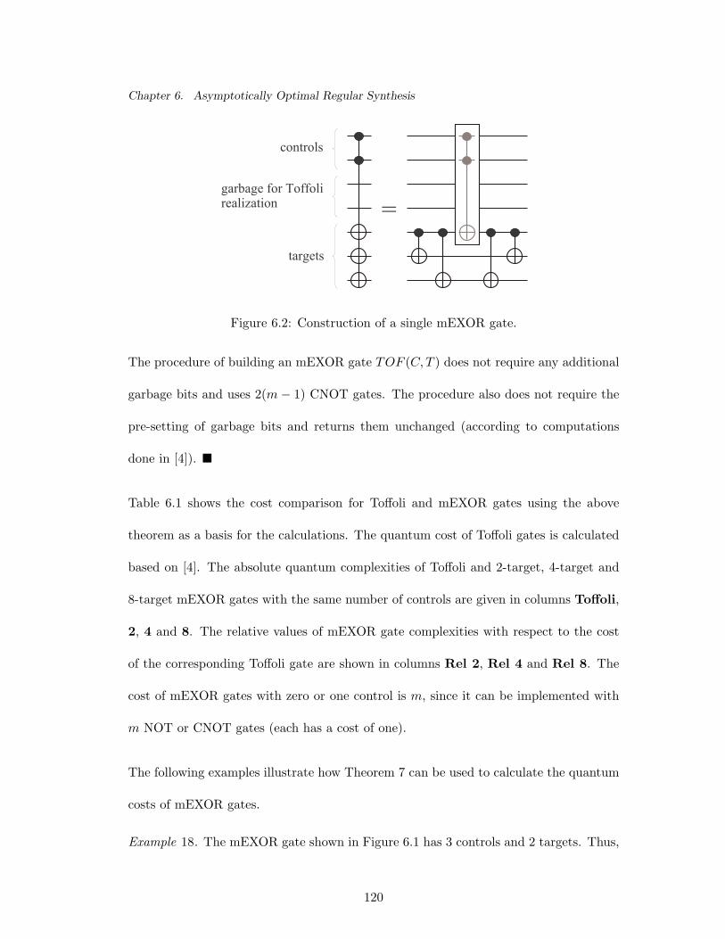
Chapter 6. Asymptotically Optimal Regular Synthesis
=
controls
garbage for Toffolirealization
targets
Figure 6.2: Construction of a single mEXOR gate.
The procedure of building an mEXOR gate TOF (C, T ) does not require any additional
garbage bits and uses 2(m − 1) CNOT gates. The procedure also does not require the
pre-setting of garbage bits and returns them unchanged (according to computations
done in [4]). ¥
Table 6.1 shows the cost comparison for Toffoli and mEXOR gates using the above
theorem as a basis for the calculations. The quantum cost of Toffoli gates is calculated
based on [4]. The absolute quantum complexities of Toffoli and 2-target, 4-target and
8-target mEXOR gates with the same number of controls are given in columns Toffoli,
2, 4 and 8. The relative values of mEXOR gate complexities with respect to the cost
of the corresponding Toffoli gate are shown in columns Rel 2, Rel 4 and Rel 8. The
cost of mEXOR gates with zero or one control is m, since it can be implemented with
m NOT or CNOT gates (each has a cost of one).
The following examples illustrate how Theorem 7 can be used to calculate the quantum
costs of mEXOR gates.
Example 18. The mEXOR gate shown in Figure 6.1 has 3 controls and 2 targets. Thus,
120
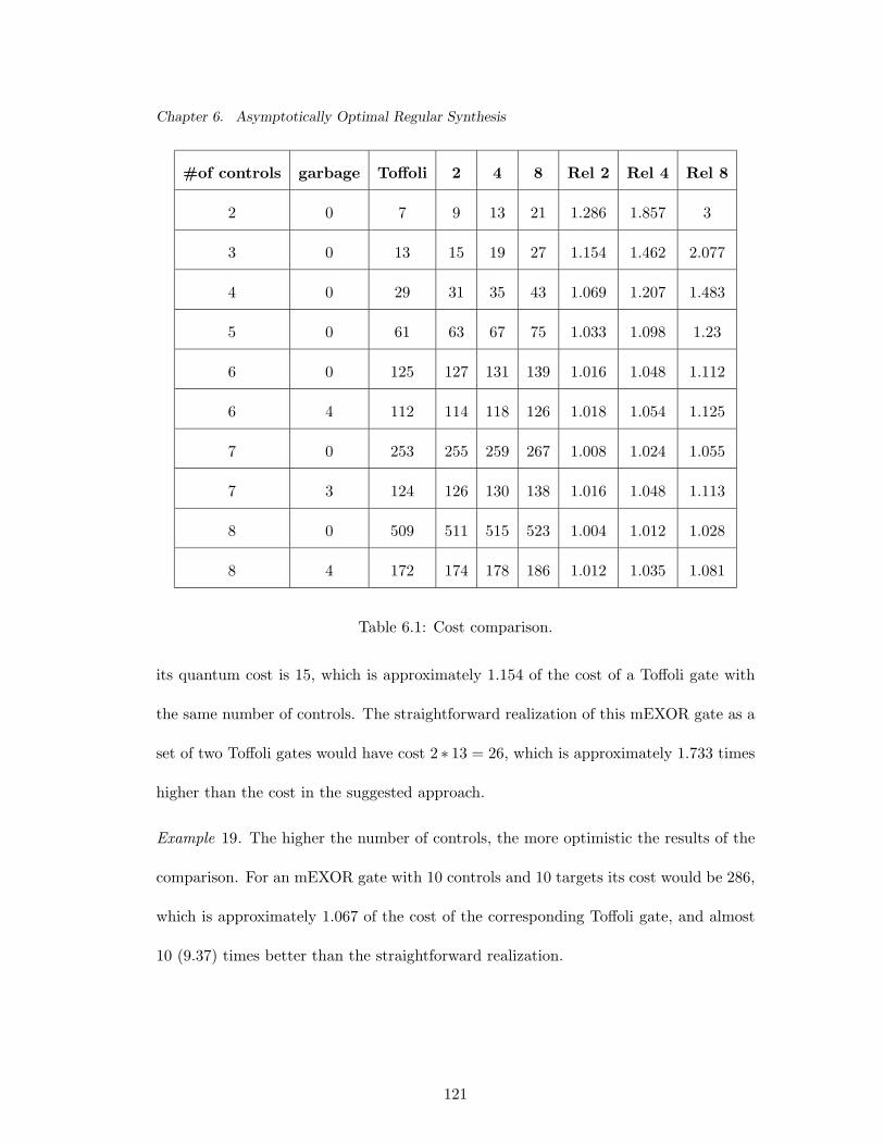
Chapter 6. Asymptotically Optimal Regular Synthesis
#of controls garbage Toffoli 2 4 8 Rel 2 Rel 4 Rel 8
2 0 7 9 13 21 1.286 1.857 3
3 0 13 15 19 27 1.154 1.462 2.077
4 0 29 31 35 43 1.069 1.207 1.483
5 0 61 63 67 75 1.033 1.098 1.23
6 0 125 127 131 139 1.016 1.048 1.112
6 4 112 114 118 126 1.018 1.054 1.125
7 0 253 255 259 267 1.008 1.024 1.055
7 3 124 126 130 138 1.016 1.048 1.113
8 0 509 511 515 523 1.004 1.012 1.028
8 4 172 174 178 186 1.012 1.035 1.081
Table 6.1: Cost comparison.
its quantum cost is 15, which is approximately 1.154 of the cost of a Toffoli gate with
the same number of controls. The straightforward realization of this mEXOR gate as a
set of two Toffoli gates would have cost 2 ∗ 13 = 26, which is approximately 1.733 times
higher than the cost in the suggested approach.
Example 19. The higher the number of controls, the more optimistic the results of the
comparison. For an mEXOR gate with 10 controls and 10 targets its cost would be 286,
which is approximately 1.067 of the cost of the corresponding Toffoli gate, and almost
10 (9.37) times better than the straightforward realization.
121
Chapter 6. Asymptotically Optimal Regular Synthesis
6.2 Asymptotically Optimal Reversible Synthesis Method
The organization of this section is as follows: we describe the reversible synthesis
method, then define the Shannon function and prove that its lower boundary has the
same cost order as the upper boundary for the cost of the algorithm. This allows us to
say that the reversible synthesis algorithm is asymptotically optimal.
The following algorithm is very similar to the modifications discussed earlier. The idea
is the usage of the Toffoli gate algorithm modification from the Chapter 4 where the
Toffoli gates with the same set of controls are united to form one mEXOR gate.
Step 0. The top part of the left side of the truth table consists of the input pattern with
the lowest order, (0, 0, ..., 0) which represents the integer 0 as a binary expression. The
corresponding pattern in the output side, (b1, b2, ..., bn) does not necessarily consist of
all zeros, therefore it must be brought to a form such that it is equal to the input part.
To do so we use one mEXOR gate, TOF (∅; bi1 , bi2 , ..., bik), where {bi1 , bi2 , ..., bik} =
{bj |bj = 1, 1 ≤ j ≤ n}.
Step k. The input part of the truth table has the pattern (a1, a2, ..., an), which
represents the binary expansion of the integer k. The output part has the pattern
(b1, b2, ..., bn) which, in general, differs from (a1, a2, ..., an). For any Boolean pattern
(x1, x2, ..., xn) we define the set X1 = {xj |xj = 1, 1 ≤ j ≤ n}, a pattern consisting of all
1-bits of (x1, x2, ..., xn). In order to bring (b1, b2, ..., bn) to the form (a1, a2, ..., an), we
need at most two mEXOR gates:
1. Increase ones. We apply mEXOR gate TOF (B1; A1 \B1) to bring (b1, b2, ..., bn)
122
Chapter 6. Asymptotically Optimal Regular Synthesis
to the form (c1, c2, ..., cn) = (a1∨b1, a2∨b2, ..., an∨bn); we change the output part
of the truth table as dictated by the gate.
2. Decrease ones. We apply mEXOR gate TOF (A1; C1\A1) to bring (c1, c2, ..., cn)
to the form (a1, a2, ..., an); we change the output part of the truth table as dictated
by the gate.
Note that during this step all the patterns previously put at their places were not altered:
• (b1, b2, ..., bn) º (a1, a2, ..., an) since all the patterns in the order less than (a1, a2, ..., an)
are already at their correct places in the upper part of the truth table.
• It follows from the definition of (c1, c2, ..., cn), (c1, c2, ..., cn) º (b1, b2, ..., bn) º
(a1, a2, ..., an) ⇒ (c1, c2, ..., cn) º (a1, a2, ..., an).
Step 2n − 1. Actually, there are no operations at the last step, since if all of the
2n − 1 patterns with lower order are on their places, there is automatically only one
spot available for the last pattern, (1, 1, ..., 1).
Complexity analysis. An upper bound on the complexity of the presented algorithm’s
output is given by the formula 2n+1 − 4. Since there are 2n steps, and each requires
at most 2 gates to be added to the network, the total cost is 2 ∗ 2n. A more accurate
analysis shows that the first step adds at most one gate, the last step never adds a gate,
and the step before last uses at most one gate (similarly to what we had in the first
step), therefore the complexity decreases to 2n+1 − 4. This bound is reachable, so it
cannot be any smaller.
Example 20. We take a reversible function given as a truth table (columns Input and
Output of the Table 6.2) with the variables named x1, x2, x3, and x4. Its output is the
123
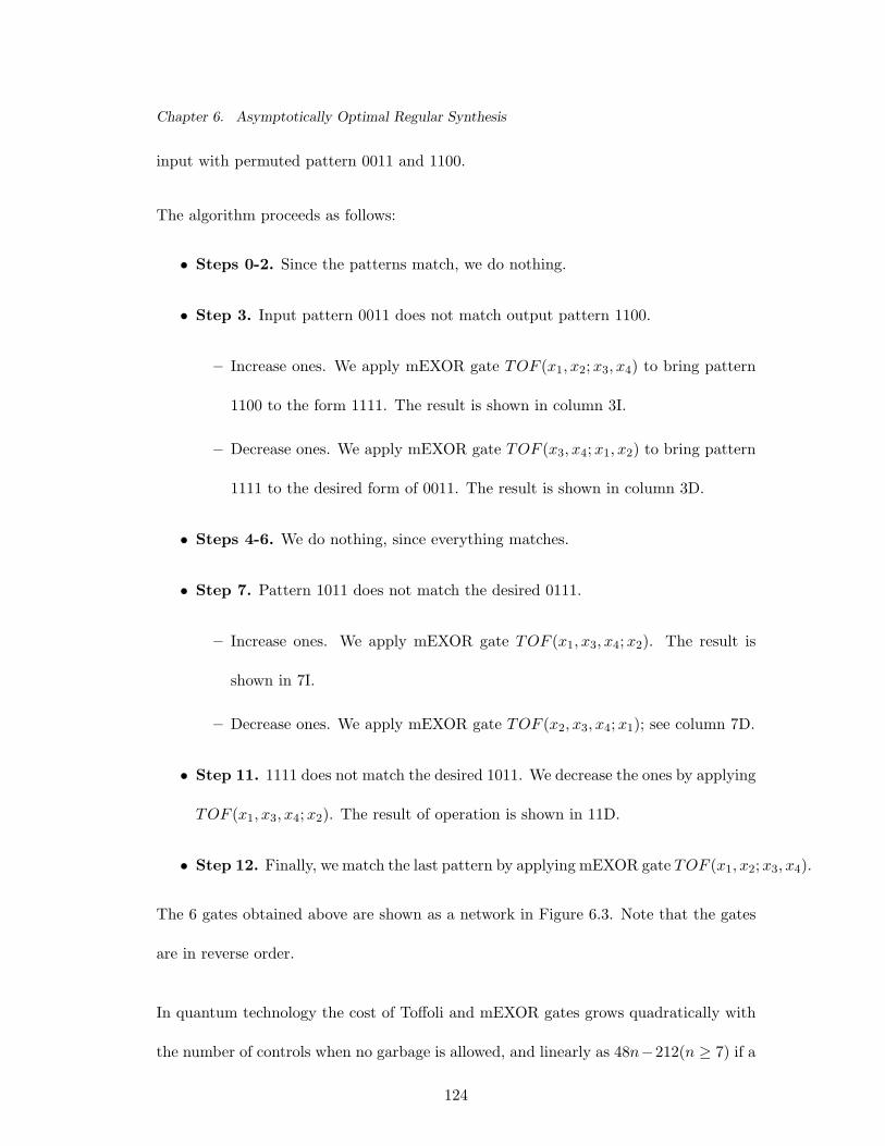
Chapter 6. Asymptotically Optimal Regular Synthesis
input with permuted pattern 0011 and 1100.
The algorithm proceeds as follows:
• Steps 0-2. Since the patterns match, we do nothing.
• Step 3. Input pattern 0011 does not match output pattern 1100.
– Increase ones. We apply mEXOR gate TOF (x1, x2; x3, x4) to bring pattern
1100 to the form 1111. The result is shown in column 3I.
– Decrease ones. We apply mEXOR gate TOF (x3, x4; x1, x2) to bring pattern
1111 to the desired form of 0011. The result is shown in column 3D.
• Steps 4-6. We do nothing, since everything matches.
• Step 7. Pattern 1011 does not match the desired 0111.
– Increase ones. We apply mEXOR gate TOF (x1, x3, x4; x2). The result is
shown in 7I.
– Decrease ones. We apply mEXOR gate TOF (x2, x3, x4; x1); see column 7D.
• Step 11. 1111 does not match the desired 1011. We decrease the ones by applying
TOF (x1, x3, x4; x2). The result of operation is shown in 11D.
• Step 12. Finally, we match the last pattern by applying mEXOR gate TOF (x1, x2; x3, x4).
The 6 gates obtained above are shown as a network in Figure 6.3. Note that the gates
are in reverse order.
In quantum technology the cost of Toffoli and mEXOR gates grows quadratically with
the number of controls when no garbage is allowed, and linearly as 48n−212(n ≥ 7) if a
124
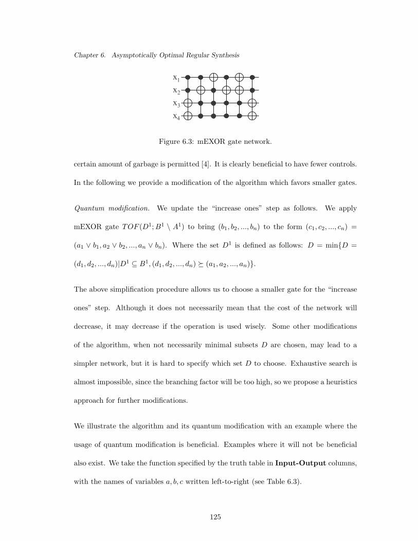
Chapter 6. Asymptotically Optimal Regular Synthesis
xxxx
1
2
3
4
Figure 6.3: mEXOR gate network.
certain amount of garbage is permitted [4]. It is clearly beneficial to have fewer controls.
In the following we provide a modification of the algorithm which favors smaller gates.
Quantum modification. We update the “increase ones” step as follows. We apply
mEXOR gate TOF (D1; B1 \ A1) to bring (b1, b2, ..., bn) to the form (c1, c2, ..., cn) =
(a1 ∨ b1, a2 ∨ b2, ..., an ∨ bn). Where the set D1 is defined as follows: D = min{D =
(d1, d2, ..., dn)|D1 ⊆ B1, (d1, d2, ..., dn) º (a1, a2, ..., an)}.
The above simplification procedure allows us to choose a smaller gate for the “increase
ones” step. Although it does not necessarily mean that the cost of the network will
decrease, it may decrease if the operation is used wisely. Some other modifications
of the algorithm, when not necessarily minimal subsets D are chosen, may lead to a
simpler network, but it is hard to specify which set D to choose. Exhaustive search is
almost impossible, since the branching factor will be too high, so we propose a heuristics
approach for further modifications.
We illustrate the algorithm and its quantum modification with an example where the
usage of quantum modification is beneficial. Examples where it will not be beneficial
also exist. We take the function specified by the truth table in Input-Output columns,
with the names of variables a, b, c written left-to-right (see Table 6.3).
125
Chapter 6. Asymptotically Optimal Regular Synthesis
For the basic approach, we find the first pattern of the output part of the truth table
which differs from the corresponding input pattern. It is 101. We increase the ones by
applying TOF (a, c; b) (result is shown in column BI), so the pattern becomes 111. We
next decrease the ones by applying TOF (b, c; a) and update the information (column
BD1). Finally, we decrease the ones of 111 to the desired input pattern 011 by applying
TOF (a, c; b).
For the quantum modification, we select the smaller gate (first step), TOF (a; b), to
increase the ones of 101 (column QI). At the second step we decrease the ones of 111
by applying TOF (b, c; a) (result is shown in QD1 column). Finally, we use TOF (a; b)
to decrease the ones of 110 to match input pattern 100.
Quantum cost analysis: the basic approach uses 3 Toffoli gates, which results in the
total cost of 21, whereas the quantum modification has cost 9.
Note that the function given in the above example can be realized with one gate, namely
the Fredkin gate.
Definition 14. The Shannon function L(n) is the maximal number of gates required
to realize a reversible function of n variables with an optimal network.
We have just proved an upper bound L(n) ≤ 2n+1 − 4, which is L(n) ∈ O(2n). We next
prove a lower bound L(n) ≥ C ∗ 2n for a positive constant C.
Lemma 13. The number of distinct mEXOR gates with n variables is (3n − 2n).
Proof. Each of the variables may participate in a gate as a control or target, or may
126
Chapter 6. Asymptotically Optimal Regular Synthesis
not be a part of a gate. This gives the possibility of 3n gates. However, among those
3n some will not contain any target bits, and therefore will not be a mEXOR gate. The
number of these last will be 2n (each bit is allowed to be either in control or is not
present). Thus, the answer is given by the formula (3n − 2n). ¥
It is interesting to note that an mEXOR gate with zero controls is used at most once in
the algorithm (Step 0), but the number of them is exponential, namely 2n. It happens
that considering these gates as a set of NOTs does not lead to a change of asymptotic
behavior, which is the focus of this section.
Theorem 8. L(n) ≥ 2n
ln 3 + o(2n).
Proof. The number of all reversible functions of n variables is 2n! (as the number of
permutations of 2n elements). The total number of mEXOR gates is 3n−2n. Supposing
that by taking all the possible cascades of mEXOR gates we get different functions
(which is, of course, not true), the complexity of the hardest to realize function is given
by the formula log(3n−2n)(2n!). Since some cascades built during such process will give
equal functions, the expression log(3n−2n)(2n!) gives a lower bound for the cost of the
most expensive to build reversible function. This expression can be simplified using
Stirling’s formula to the form 2n
ln 3 + o(2n). ¥
6.3 Conclusion
In this chapter the first asymptotically optimal algorithm in reversible logic synthe-
sis theory was presented. The results of this section are mostly theoretical, although
they may be used in applications. This is the first (in literature) result on asymptotic
127
Chapter 6. Asymptotically Optimal Regular Synthesis
optimality of the gate count in a reversible synthesis procedure.
128
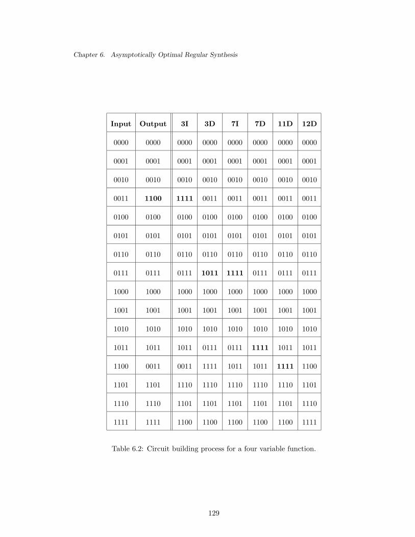
Chapter 6. Asymptotically Optimal Regular Synthesis
Input Output 3I 3D 7I 7D 11D 12D
0000 0000 0000 0000 0000 0000 0000 0000
0001 0001 0001 0001 0001 0001 0001 0001
0010 0010 0010 0010 0010 0010 0010 0010
0011 1100 1111 0011 0011 0011 0011 0011
0100 0100 0100 0100 0100 0100 0100 0100
0101 0101 0101 0101 0101 0101 0101 0101
0110 0110 0110 0110 0110 0110 0110 0110
0111 0111 0111 1011 1111 0111 0111 0111
1000 1000 1000 1000 1000 1000 1000 1000
1001 1001 1001 1001 1001 1001 1001 1001
1010 1010 1010 1010 1010 1010 1010 1010
1011 1011 1011 0111 0111 1111 1011 1011
1100 0011 0011 1111 1011 1011 1111 1100
1101 1101 1110 1110 1110 1110 1110 1101
1110 1110 1101 1101 1101 1101 1101 1110
1111 1111 1100 1100 1100 1100 1100 1111
Table 6.2: Circuit building process for a four variable function.
129
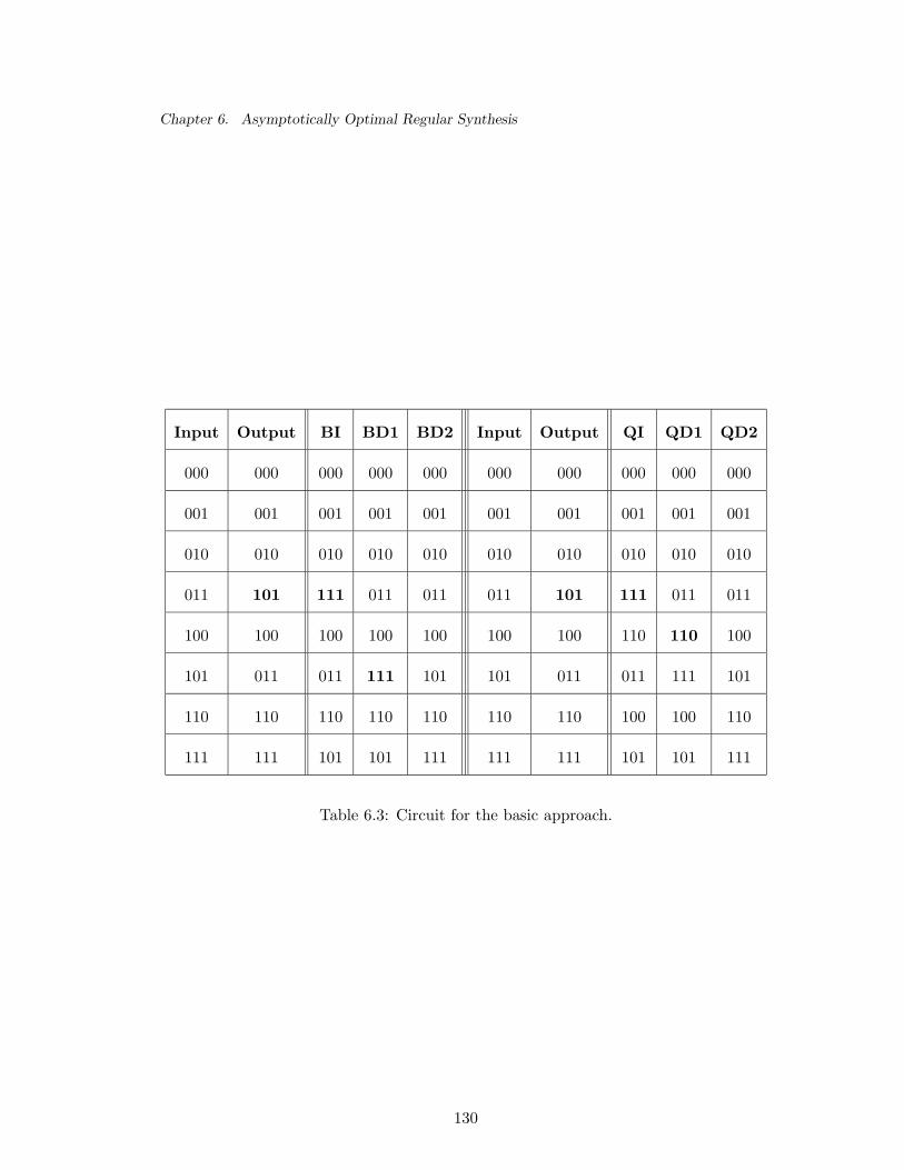
Chapter 6. Asymptotically Optimal Regular Synthesis
Input Output BI BD1 BD2 Input Output QI QD1 QD2
000 000 000 000 000 000 000 000 000 000
001 001 001 001 001 001 001 001 001 001
010 010 010 010 010 010 010 010 010 010
011 101 111 011 011 011 101 111 011 011
100 100 100 100 100 100 100 110 110 100
101 011 011 111 101 101 011 011 111 101
110 110 110 110 110 110 110 100 100 110
111 111 101 101 111 111 111 101 101 111
Table 6.3: Circuit for the basic approach.
130
Chapter 7Dynamic Programming Algorithms asReversible Circuits: SymmetricFunction Realization
In this chapter we give a general idea of how to realize a dynamic programming algorithm
as a reversible circuit. This realization is not tied to a specific reversible design model
and technology or a class of dynamic algorithms; it shows an approach for such synthesis.
As an illustration of this approach, a class of all symmetric functions is realized in a
dynamic programming algorithm manner as a reversible circuit of Toffoli elements. The
garbage, quantum and reversible costs of the presented implementation are calculated
and compared to the costs of previously described reversible synthesis methods (both
the reversible synthesis methods presented in this thesis, as well as those presented in
works of other authors).
General recursion and dynamic programming algorithms [9, 17, 19] form a very impor-
tant class of algorithms. Many real-world problems can be solved by dynamic program-
ming algorithms: finding a value for a symmetric function, algorithms on strings, and
most approximation methods.
The main idea of a dynamic programming algorithm is the recursive decomposition of
131
Chapter 7. Dynamic Programming Algorithms as Reversible Circuits: Symmetric Function Realization
the problem f into a set of other problems, where the answer for f can be found in terms
of a “simple” operation on the answers of subproblems. When the dynamic algorithm is
completely specified, a set of operations needed to make a step of the calculation, and a
set of subfunctions needed for the computation is defined. Further, to build a reversible
circuit we will realize each of the algorithm operations as a reversible cascade. But first,
we need to find the garbage cost of the implementation.
Given a problem (function) f with Boolean inputs (x1, x2, ..., xn) and a dynamic algo-
rithm that terminates after S steps of calculation, we first calculate the two numbers:
• M = maxs=1..S(ms), where ms is the number of Boolean values (intermediate
storage) needed in addition to the input values in order to complete the calculation
starting at step s. That is, M represents the maximum number of subfunction
values which are needed in order to complete the algorithm calculation starting
from step s. For simplicity assume that on each step of the algorithm only one
subfunction value is updated.
• Given a reversible design model and the set of all operations the dynamic algorithm
performs at one step, we find the number G = maxs=1..S(gs), where gs is the
minimal amount of garbage needed for the reversible implementation of the s-th
step of the algorithm in terms of the considered model.
When the two numbers are determined, the circuit is constructed as follows:
• We create the set of input constants size M + G and assign zero values to all
of them. M will be used to store intermediate results of the calculation and the
answer itself, and the G values are needed for the calculation.
132
Chapter 7. Dynamic Programming Algorithms as Reversible Circuits: Symmetric Function Realization
• We use the reversible design model to create a circuit for each of the S steps of the
specified dynamic programming algorithm. The circuit changes one subfunction
value at a time.
When the circuit is built, the outputs which contain the answer are specified by the
dynamic algorithm.
The amount of the resulting reversible design garbage, as well as the final cost of the
network will depend on the design of the dynamic programming algorithm and strength
of the reversible design model.
Note that a benefit of using this method comes from the following consideration. If a
multiple output function to be realized has outputs for which the dynamic program-
ming algorithm is known and those for which the dynamic programming algorithm
is not known, the dynamic programming realizable outputs can be built first by the
suggested method. The resulting circuit passes the input values through unchanged.
Therefore, the remaining outputs can be built by any other procedure without any
special preprocessing.
7.1 Application: Multiple Output Symmetric Functions
To run the application, we need reversible logic gates (design model), a synthesis model,
and the dynamic programming algorithm. We define the model by taking the most
popular of reversible logic gates: TOF (a), TOF (a; b), and TOF (a, b; c). The set of
these gates was shown to be complete. This is a minimally complete set of gates in the
sense that excluding any one from this set will result in incompleteness if no garbage
133

Chapter 7. Dynamic Programming Algorithms as Reversible Circuits: Symmetric Function Realization
addition is allowed. We do not choose any specific design procedure as it will be showed
that the implementation of a single step of the dynamic programming algorithm is very
simple.
To design a dynamic programming algorithm we need several definitions.
Definition 15. Multiple output symmetric Boolean function−→F (x1, x2, ..., xn) =
(y1, y2, ..., ym) is such a function that−→F (x1, x2, ..., xn) =
−→F (π(x1, x2, ..., xn)), where π
is a permutation of n elements.
Definition 16. The σ-function σkn(x1, x2, ..., xn) is defined as
⊕{i1<i2<...<ik} xi1xi2 ...xik
for k = 0, 1, ..., n.
Lemma 14. Every symmetric function can be written as a linear combination (with
respect to operation EXOR) of not more than (n + 1) σ-functions.
Proof. There are (n+1) different σ-functions; all are linearly independent. In fact, their
kernels (set of inputs such that for each input the function is not equal to zero) do not
intersect, thus different linear combinations produce different functions. All σ-functions
are symmetric, and so are their linear combinations. The number of symmetric functions
of n variables is 2n+1, therefore the different linear combinations of σ-functions form
the set of all symmetric functions and each symmetric function has a unique linear form
made of σ-functions. ¥
Lemma 15. σkn(x1, x2, ..., xn) = xnσk−1
n−1(x1, x2, ..., xn−1) ⊕ σkn−1(x1, x2, ..., xn−1) for k ≥
2.
134

Chapter 7. Dynamic Programming Algorithms as Reversible Circuits: Symmetric Function Realization
Proof. Observe that the first part of the right hand side has all the terms of degree
k which include variable xn as a multiple, while the second part has all the terms of
degree k which do not include the variable xn. Thus, the right hand side has all the
terms of degree k, which, by definition, forms the left hand side. ¥
Note that the statement of Lemma 15 holds for k = 1. The result for k = 1 will be used to
calculate σ1n(x1, x2, ..., xn). Use Lemma 15 to form the dynamic programming algorithm
for calculating a symmetric function by saying that in order to build a multiple output
symmetric function, we first build the set of σ-functions recursively and then construct
the output vector as a linear combination of the outputs of dynamic programming
algorithm. Formally the algorithm works as follows:
1. create Boolean array sigma[1..n]=0;
2. for i=1 to n
3. for k=i down to 1
4. if k>1 sigma[k] = (sigma[k] + x[i]*sigma[k-1]) mod 2;
5. if k=1 sigma[k] = (sigma[k] + x[i]) mod 2;
6. end for;
7. end for.
We define the two numbers needed for calculation and build the circuit:
• In order to calculate σab (x1, x2, ..., xb) we need σa−1
b−1 (x1, x2, ..., xb−1) and σab−1(x1, x2, ..., xn),
and in order to continue and complete the calculations we will need σa−1b−1 (x1, x2, ..., xb−1),
σa−2b−1 (x1, x2, ..., xb−1), ..., σ1
b−1(x1, x2, ..., xb−1). If a = 1, we use the formula σ1b (x1, x2, ..., xb) =
σ1b−1(x1, x2, ..., xb−1)⊕xb. For a = 0 we do not create anything, since the addition
135
Chapter 7. Dynamic Programming Algorithms as Reversible Circuits: Symmetric Function Realization
of a unit can be done in-place when the outputs are created by a single NOT gate.
Therefore, M = maxb=1,2,...,n(b) = n.
• For the intermediate calculations no garbage is needed, G=0. To calculate func-
tion σ1b (x1, x2, ..., xb) we use the gate TOF (xb; σ1
b−1(x1, x2, ..., xb−1)) at line 4 of the
pseudocode. The function σ1b−1(x1, x2, ..., xb−1) will not be used in further calcu-
lations, so we can overwrite it. To calculate σab (x1, x2, ..., xb), we use the gate
TOF (xb, σab−1(x1, x2, ..., xn);σa−1
b−1 (x1, x2, ..., xb−1)) at line 5 of the pseudocode.
Again, the function σa−1b−1 (x1, x2, ..., xb−1) will not be used in further calculations,
so we can overwrite it.
When the dynamic programming part creates the set of outputs σkn(x1, x2, ..., xn) for
k = 1, 2, .., n, we construct the output by including the needed σ-functions. Depending
on what the function is, we may or may not need to create the additional garbage
outputs. A greedy method may create m additional zero constants for the outputs. In
practice, a better solution is usually possible. The described synthesis algorithm allows
to formulate the following result.
Theorem 9. Every symmetric multiple output function−→F (x1, x2, ..., xn) = (y1, y2, ..., ym)
can be realized with the cost of:
• at most m NOT gates, at most n + mn CNOT gates, and n(n−1)2 Toffoli gates;
• garbage of at most 2n bits.
Less garbage can be achieved if we notice that there is no need to create a special con-
stant line for σ1b (x1, x2, ..., xb), which can be stored on the input line xb. This allows us to
136

Chapter 7. Dynamic Programming Algorithms as Reversible Circuits: Symmetric Function Realization
decrease both garbage and reversible implementation costs by 1. Other garbage and cost
saving comes from the observation that if all the outputs can be composed of the first
k + 1 (2 ≤ k ≤ n) σ-functions σ0n(x1, x2, ..., xn), σ1
n(x1, x2, ..., xn), ..., σkn(x1, x2, ..., xn),
we do not need to run the dynamic programming algorithm to create the remaining
(n − k) σ-functions. These two observations allow us to formulate the following result:
Theorem 10. Every symmetric multiple output function−→F (x1, x2, ..., xn) = (y1, y2, ..., ym),
where a linear σ-function decomposition requires a function of maximal degree k
(2 ≤ k ≤ n) can be realized with the cost of:
• at most m NOT gates, at most n+mn−1 CNOT gates, and (2n−k)(k−1)2 Toffoli
gates;
• garbage of at most n + k − 1 bits.
Another benefit of using this method comes from the following consideration. If a
multiple output function to be realized has both symmetric and non symmetric outputs,
the symmetric outputs can be realized first by the suggested method. Then, the set
of gates TOF (xn−1; xn) TOF (xn−2; xn−1) ... TOF (x2; x1) is applied to the end of the
cascade, which creates the whole set of unchanged inputs {x1, x2, ..., xn} on the first
n output lines of the cascade. Therefore, the remaining outputs can be built by any
other procedure. Such an operation adds (n− 1) gates to the cascade. If for the target
technology the cost of a single garbage bit is less than the cost of (n− 2) CNOT gates,
the very first approach when a special line is created for σ1(x1, x2, ..., xn) can be used.
Example 21. Take a multiple output function rd53.pla, which is the 5-input 3-output
symmetric function whose output is the binary representation of the number of ones in
137
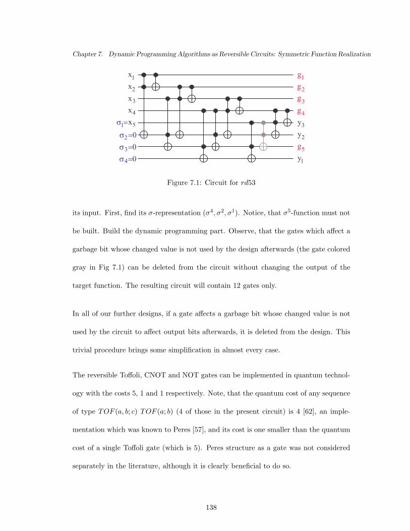
Chapter 7. Dynamic Programming Algorithms as Reversible Circuits: Symmetric Function Realization
xxxxx
s =0s =0s =0
1
2
3
4
5
2
3
4
s =1
g
gggg12
3
4
5
1
2
3
y
yy
Figure 7.1: Circuit for rd53
its input. First, find its σ-representation (σ4, σ2, σ1). Notice, that σ5-function must not
be built. Build the dynamic programming part. Observe, that the gates which affect a
garbage bit whose changed value is not used by the design afterwards (the gate colored
gray in Fig 7.1) can be deleted from the circuit without changing the output of the
target function. The resulting circuit will contain 12 gates only.
In all of our further designs, if a gate affects a garbage bit whose changed value is not
used by the circuit to affect output bits afterwards, it is deleted from the design. This
trivial procedure brings some simplification in almost every case.
The reversible Toffoli, CNOT and NOT gates can be implemented in quantum technol-
ogy with the costs 5, 1 and 1 respectively. Note, that the quantum cost of any sequence
of type TOF (a, b; c) TOF (a; b) (4 of those in the present circuit) is 4 [62], an imple-
mentation which was known to Peres [57], and its cost is one smaller than the quantum
cost of a single Toffoli gate (which is 5). Peres structure as a gate was not considered
separately in the literature, although it is clearly beneficial to do so.
138
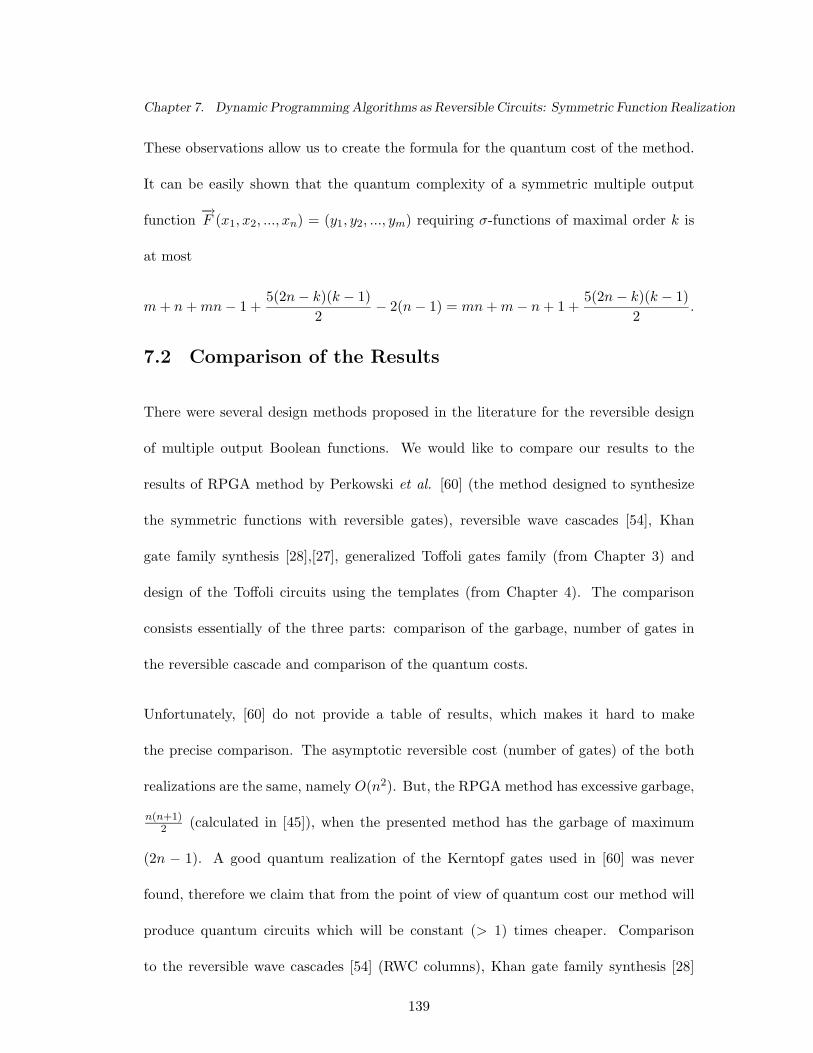
Chapter 7. Dynamic Programming Algorithms as Reversible Circuits: Symmetric Function Realization
These observations allow us to create the formula for the quantum cost of the method.
It can be easily shown that the quantum complexity of a symmetric multiple output
function−→F (x1, x2, ..., xn) = (y1, y2, ..., ym) requiring σ-functions of maximal order k is
at most
m + n + mn − 1 +5(2n − k)(k − 1)
2− 2(n − 1) = mn + m − n + 1 +
5(2n − k)(k − 1)2
.
7.2 Comparison of the Results
There were several design methods proposed in the literature for the reversible design
of multiple output Boolean functions. We would like to compare our results to the
results of RPGA method by Perkowski et al. [60] (the method designed to synthesize
the symmetric functions with reversible gates), reversible wave cascades [54], Khan
gate family synthesis [28],[27], generalized Toffoli gates family (from Chapter 3) and
design of the Toffoli circuits using the templates (from Chapter 4). The comparison
consists essentially of the three parts: comparison of the garbage, number of gates in
the reversible cascade and comparison of the quantum costs.
Unfortunately, [60] do not provide a table of results, which makes it hard to make
the precise comparison. The asymptotic reversible cost (number of gates) of the both
realizations are the same, namely O(n2). But, the RPGA method has excessive garbage,
n(n+1)2 (calculated in [45]), when the presented method has the garbage of maximum
(2n − 1). A good quantum realization of the Kerntopf gates used in [60] was never
found, therefore we claim that from the point of view of quantum cost our method will
produce quantum circuits which will be constant (> 1) times cheaper. Comparison
to the reversible wave cascades [54] (RWC columns), Khan gate family synthesis [28]
139
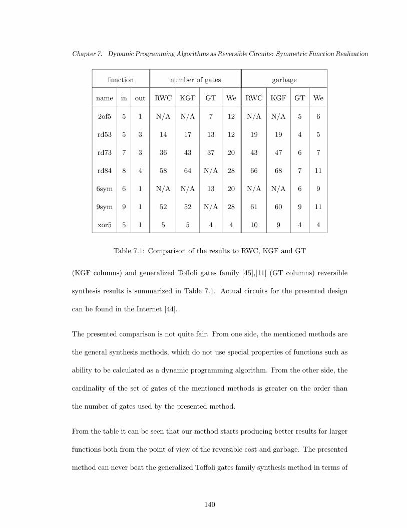
Chapter 7. Dynamic Programming Algorithms as Reversible Circuits: Symmetric Function Realization
function number of gates garbage
name in out RWC KGF GT We RWC KGF GT We
2of5 5 1 N/A N/A 7 12 N/A N/A 5 6
rd53 5 3 14 17 13 12 19 19 4 5
rd73 7 3 36 43 37 20 43 47 6 7
rd84 8 4 58 64 N/A 28 66 68 7 11
6sym 6 1 N/A N/A 13 20 N/A N/A 6 9
9sym 9 1 52 52 N/A 28 61 60 9 11
xor5 5 1 5 5 4 4 10 9 4 4
Table 7.1: Comparison of the results to RWC, KGF and GT
(KGF columns) and generalized Toffoli gates family [45],[11] (GT columns) reversible
synthesis results is summarized in Table 7.1. Actual circuits for the presented design
can be found in the Internet [44].
The presented comparison is not quite fair. From one side, the mentioned methods are
the general synthesis methods, which do not use special properties of functions such as
ability to be calculated as a dynamic programming algorithm. From the other side, the
cardinality of the set of gates of the mentioned methods is greater on the order than
the number of gates used by the presented method.
From the table it can be seen that our method starts producing better results for larger
functions both from the point of view of the reversible cost and garbage. The presented
method can never beat the generalized Toffoli gates family synthesis method in terms of
140

Chapter 7. Dynamic Programming Algorithms as Reversible Circuits: Symmetric Function Realization
garbage, since the last has theoretically minimal garbage. But, the GT method scales
badly, it can produce the circuits for reversible functions with no more than 10 inputs.
The RWC and KGF are synthesized heuristically and they also scale much worse than
the presented method.
Quantum cost comparison can be done accurately but in this paper we just mention
that the quantum cost of RWC is at least n times reversible design cost, quantum cost
of KGF implementation is at least 2n times higher than its reversible cost and quantum
cost of GT is at least n times higher than its reversible cost, where n is the number of
inputs of a function. The quantum cost for our model is given in previous section, and
it cannot exceed 5 times the reversible cost. Clearly, the quantum cost of the presented
approach is much better.
To illustrate how good the quantum cost is, compare the results to the ones presented
in Chapter 4. This chapter provides an example of a circuit for rd53.pla function
which has a cost of 12 gates, which seem to be the best among all known in reversible
logic synthesis. The generalized Toffoli gates used in Chapter 4 are expensive (but no
more expensive than the gates in RWC, KGF and GT) and the quantum complexity
calculation based on results of [4] gives the quantum cost of 132 for that realization.
Although the realization of rd53.pla presented in this paper has 12 gates in the reversible
model, its quantum cost is only 36. Relation of the quantum costs 11:3 clearly shows
the benefits of using the dynamic algorithm reversible synthesis method even for small
functions. Since our method produces better results for larger functions, the quantum
cost comparison for them will be even more beneficial.
141
Chapter 7. Dynamic Programming Algorithms as Reversible Circuits: Symmetric Function Realization
Another interesting comparison can be made using 2of5.pla function. GT realization
claims 7 gates only in comparison to 12 in the presented paper. However, the quantum
cost of GT realization is 158 in comparison to 32 for our circuit with 12 gates.
7.3 Conclusion
In this chapter we presented a general approach to the synthesis of reversible circuits
for the dynamic programming problems. As an illustration of its efficiency we applied
it to the set of all multiple output symmetric functions and analyzed the three cost
factors: reversible model cost, garbage cost and quantum cost. We showed that almost
in every possible comparison our method produces better results (except for garbage
comparison with RCMG and Toffoli synthesis). The garbage in the presented method
is close to the theoretical minimum. The quantum cost of the circuits produced by the
new algorithm is always significantly better. Finally, due to the small size of the gates
used (maximum 3 inputs and 3 outputs), the levels of the network can be compressed
which will result in a further simplification. On the contrary, it is unlikely that the level
compression operation will give good results for models that use large gates.
142

Chapter 8Summary
The thesis starts with analysis of garbage in existing reversible design models. My
first point is that excessive amounts of garbage are introduced by existing synthesis
approaches. Given that garbage is very expensive for some of the technologies that use
reversibility, a question arises: is it possible to synthesize functions with less garbage
(if not absolutely minimal) using gates of a reasonable technological cost and with
relatively small circuits? Chapter 3 provides a complete answer to this question. A new
structure, initially intended for reversible synthesis with theoretically minimal garbage
was created and the synthesis algorithm was developed. The cost of a single gate was
analyzed, and shown to be only marginally higher than the cost of the conventional
Toffoli gate. The heuristic synthesis of a new model produces results comparable to
the synthesis of other reversible circuits. The new RCMG model was shown to be
superior to the conventional non-reversible synthesis of EXOR PLAs both practically
and theoretically. The practical part has circuits for rd53.pla and a 3-bit full adder
that are smaller than the corresponding EXOR PLA realizations. The theoretical part
consists of two results. First, given an EXOR PLA, the RCMG circuit with the number
of gates equal to the number of terms of EXOR PLA was constructed. Second, a class
of exponentially hard to realize as EXOR PLAs functions was found. These functions
143
Chapter 8. Summary
can be realized with only a linear gate count (cost) by the RCMG model. Also, if the
technology allows compressing of levels, the cost becomes a constant(!).
Next, I tried a different approach, where a circuit is initially created by a regular syn-
thesis algorithm, and the created circuit is usually smaller than the one created by the
RCMG regular synthesis algorithm. Then, a template simplification tool was applied.
In this approach only Toffoli and Fredkin gates were used as the gates for which a good
implementation was found. In comparison to the results of RCMG synthesis I obtained
better circuits for the new reversible specifications. For small reversible functions our
algorithm behaves close to optimal by producing circuits that are only 105.9% more ex-
pensive than the optimal. Unfortunately, the new method does not handle “don’t cares”.
Currently, we are working on handling “don’t cares”, extending the set of model gates
and polishing up the template tool.
An interesting theoretical result would be an asymptotically optimal synthesis method.
Such a method was found, and the model gates for the synthesis of this method were
shown to be only marginally higher than the cost of Toffoli gates.
Finally, dynamic programming algorithms were realized in a reversible manner. Since
the set of all dynamic programming algorithms is complex, this section has only a the-
oretical method for a general solution. As an application I considered the class of all
multiple output symmetric functions, elements of which were shown to be dynamic pro-
gramming algorithms. This class was realized in a reversible manner and the results of
the circuit cost comparison to other synthesis methods showed that even a straightfor-
ward application of the theoretical algorithm produces the best known circuits.
144
Chapter 9Further Research
Results of the presented thesis form the basis for further research. Currently, several
topics need more investigation.
1. The template tool can be applied to simplify the structure of an RCMG network.
Essentially, an RCMG gate is a Toffoli gate, for which a search of the templates
was done in Chapter 4. The results of this chapter can be taken as a start of the
search for more generalized templates. The same idea (a template simplification
tool) can be generalized to simplify the mEXOR gate network, as well as the
hybrid RCMG-mEXOR model.
2. In quantum technology there are essentially quantum gates, such as X (analogy of
Boolean NOT), Z and Hadamard gate, whose specification cannot be considered
from the point of view of Boolean logic only. However, these gates have the
property needed to use them in templates: they are all self-inverses. Rotation
gates are among the quantum gates that are not self inverses. However, they
can be incorporated into the template structure by generalizing the template as
follows (to be generalized). The generalized template of size m is the cascade
of gates G0 G1...Gm−1 which realizes the identity function. Any template of size
145

Chapter 9. Further Research
m should be independent of smaller size templates, i.e. application of smaller size
templates does not decrease the number of gates in a size m template. Given a
template G0 G1...Gm−1, its application for parameter k such that m/2 ≤ k ≤ m
and any i such that 0 ≤ i ≤ m is:
Gi G(i+1) mod m... G(i+k−1) mod m → G(i−1) mod m G(i−2) mod m... G(i+k) mod m
Such a template tool will allow simplification of any quantum network.
3. The synthesis algorithms in Chapters 4, 5, 6 do not use a look-ahead technique to
produce initially smaller circuits. It would be useful to investigate this modifica-
tion. One more modification is a one-directional synthesis with “don’t cares”. It
should be relatively easy to describe and test such an algorithm.
4. The Miller gate can be easily and naturally incorporated into the synthesis al-
gorithm of Chapter 5. The problems with the Miller gate will appear when new
templates will be needed; the new template classification may be harder.
5. The dynamic programming algorithm reversible circuits were built only for sym-
metric functions. It is worth looking at other important dynamic algorithms and
try to realize them as reversible circuits. The resulting circuits for this approach
are expected to scale well and be small due to their use of information on the
general structure of the target function.
6. Expansion of the table of optimal circuits for functions of 4 variables. This cannot
be done in a straightforward manner, a and classification of reversible functions
is required. Some other reductions should also be investigated. This may initially
sound a bit strange, as why would one be interested in all optimal size 4 reversible
146
Chapter 9. Further Research
functions from the point of view of possible applications? However, in addition to
a better understanding of reversible logic, this work will produce some applicable
results. For instance, cellular arrays require synthesis of size 4 reversible functions
only.
7. Synthesis procedures based on the truth table are limited to functions of, say, 30
inputs (if usage of modern computers for CAD is expected). Thus, a new design
procedures needed. It may be useful to search for synthesis procedures based on
the function factorization and theory of the group of permutations.
147
Bibliography
[1] IBM’s test-tube quantum computer makes history. Technical report,
http://researchweb.watson.ibm.com/resources/news/20011219 quantum.shtml,
Dec. 2001.
[2] A. Al-Rabadi. Novel Methods for Reversible Logic Synthesis and Their Application
to Quantum Computing. PhD thesis, Portland State University, Portland, Oregon,
USA, October 2002.
[3] W. C. Athas and L. J. Svensson. Reversible logic issues in adiabatic CMOS.
[4] A. Barenco, C. H. Bennett, R. Cleve, D. P. DiVinchenzo, N. Margolus, P. Shor,
T. Sleator, J. A. Smolin, and H. Weinfurter. Elementary gates for quantum com-
putation. The American Physical Society, 52:3457–3467, 1995.
[5] C. H. Bennett. Logical reversibility of computation. IBM J. Research and Devel-
opment, 17:525–532, November 1973.
[6] C. H. Bennett. Notes on the history of reversible computation. IBM J. Research
and Development, 32(1):16–23, January 1988.
[7] D. Brand and T. Sasao. Minimization of AND-EXOR expressions using rewriting
rules. IEEE Transactions on Computers, 42(5):568–576, May 1993.
[8] J. W. Bruce, M. A. Thornton, L. Shivakumaraiah, P. S. Kokate, and X. Li. Efficient
adder circuits based on a conservative reversible logic gate. In IEEE Symposium
on VLSI, pages 83–88, April 2002.
[9] T. H. Cormen, C. E. Leiserson, and R. L. Rivest. Introduction to Algorithms. The
MIT Press, Cambridge, Massachusetts, 1990.
[10] B. Desoete, A. De Vos, M. Sibinski, and T. Widerski. Feynman’s reversible gates
implemented in silicon. In 6th International Conference MIXDES, pages 496–502,
1999.
148
Bibliography
[11] G. W. Dueck and D. Maslov. Reversible function synthesis with minimum garbage
outputs. In 6th International Symposium on Representations and Methodology of
Future Computing Technologies, pages 154–161, March 2003.
[12] G. W. Dueck, D. Maslov, and D. M. Miller. Transformation-based synthesis of
networks of Toffoli/Fredkin gates. In IEEE Canadian Conference on Electrical
and Computer Engineering, Montreal, Canada, May 2003.
[13] R. Feynman. Quantum mechanical computers. Optic News, 11:11–20, 1985.
[14] E. Fredkin and T. Toffoli. Conservative logic. International Journal of Theoretical
Physics, 21:219–253, 1982.
[15] A. Gaidukov. Algorithm to derive minimum ESOP for 6-variable function. In 5th
International Workshop on Boolean Problems, pages 141–148, September 2002.
[16] N. Gershenfeld and I. L. Chuang. Quantum computing with moleculas. Scientific
American, June 1998.
[17] M. T. Goodrich and R. Tamassia. Algorithm Design: foundations, analysis, and
Internet Examples. John Wiley & Sons, Inc., 2002.
[18] G. Hinton, D. Sager, M. Upton, D. Boggs, D. Carmean, A. Kyker, and P. Rous-
sel. The microarchitecture of the Pentium 4 processor. Technical report, Intel
Technology Journal, 2001.
[19] E. Horowitz, S. Sahni, and S. Rajasekaran. Computer Algorithms/C++. Computer
Science Press, 1998.
[20] Richard J. Hughes. A technology roadmap for quantum computing and communi-
cations. In DAC, http://qist.lanl.gov/, June 2003.
[21] S. L. Hurst, D. M. Miller, and J. C. Muzio. Spectral Techniques in Digital Logic.
Academic Press, Orlando, Florida, 1985.
[22] K. Iwama, Y. Kambayashi, and S. Yamashita. Transformation rules for designing
CNOT-based quantum circuits. In Design Automation Conference, New Orleans,
Louisiana, USA, June 10-14 2002.
149

Bibliography
[23] P. Kerntopf. A comparison of logical efficiency of reversible and conventional gates.
In International Workshop on Logic Synthesis, pages 261–269, 2000.
[24] P. Kerntopf. Maximally efficient binary and multi-valued reversible gates. In Inter-
national Workshop on Post-Binary ULSI Systems, pages 55–58, Warsaw, Poland,
May 2001.
[25] P. Kerntopf. Synthesis of multipurpose reversible logic gates. In EUROMICRO
Symposium on Digital Systems Design, pages 259–266, 2002.
[26] R. W. Keyes and R. Landauer. Minimal energy dissipation in logic. IBM J. Research
and Development, pages 152–157, March 1970.
[27] M. H. A. Khan and M. Perkowski. Logic synthesis with cascades of new reversible
gate families. In 6th International Symposium on Representations and Methodology
of Future Computing Technology (Reed-Muller), pages 43–55, March 2003.
[28] M. H. A. Khan and M. Perkowski. Multi-output ESOP synthesis with cascades
of new reversible gate family. In 6th International Symposium on Representations
and Methodology of Future Computing Technologies, pages 144–153, March 2003.
[29] A. Khlopotine, M. Perkowski, and P. Kerntopf. Reversible logic synthesis by it-
erative compositions. International Workshop on Logic Synthesis, pages 261–266,
2002.
[30] J. Kim. A study on Ensemble Quantum Computers. PhD thesis, Korea Advanced
Institute of Science and Technology, Korea, May 2002.
[31] J. Kim, J.-S. Lee, and S. Lee. Implementation of the refined Deutsch-Jozsa algo-
rithm on a three-bit NMR quantum computer. Physical Review A, 62, 2000.
[32] J. Kim, J.-S. Lee, and S. Lee. Implementing unitary operators in quantum compu-
tation. Physical Review A, 62, 2000.
[33] K. Kinoshita, T. Sasao, and J. Matsuda. On magnetic bubble logic circuits. IEEE
Transactions on Comput., C-25(3):247–253, March 1976.
150

Bibliography
[34] R. Landauer. Irreversibility and heat generation in the computing process. IBM
J. Research and Development, 5:183–191, 1961.
[35] J.-S. Lee, Y. Chung, J. Kim, and S. Lee. A prectical method of constructing
quantum combinatorial logic circuits. Technical report, November 1999.
[36] M. Lukac, M. Pivtoraiko, A. Mishchenko, and M. Perkowski. Automated synthesis
of generalized reversible cascades using genetic algorithms. In 5th International
Workshop on Boolean Problems, pages 33–45, Freiburg, Germany, September 2002.
[37] O. B. Lupanov. Schemes with the finite fan-outs. Problemy Kibernetiki. Fizmatgiz,
Moscow (in Russian).
[38] N. Margolus. Feynman and Computation, chapter Crystalline Computation.
Perseus Books, 1999.
[39] D. Maslov and G. Dueck. Asymptotically optimal regular synthesis of reversible
networks. In International Workshop on Logic Synthesis, pages 226–231, Laguna
Beach, CA, 2003.
[40] D. Maslov and G. Dueck. Complexity of reversible Toffoli cascades and EXOR
PLAs. In 12th International Workshop on Post-Binary ULSI Systems, pages 17–
20, Japan, May 2003.
[41] D. Maslov, G. Dueck, and M. Miller. Fredkin/Toffoli templates for reversible logic
synthesis. In International Conference on Computer Aided Design, November 2003.
[42] D. Maslov, G. Dueck, and M. Miller. Templates for Toffoli network synthesis. In
International Workshop on Logic Synthesis, pages 320–326, Laguna Beach, CA,
2003.
[43] D. Maslov, G. Dueck, and M.Miller. Simplification of Toffoli networks via tem-
plates. In Symposium on Integrated Circuits and System Design, September 2003.
[44] D. Maslov, G. Dueck, and N. Scott. Reversible logic synthesis benchmarks page.
Technical report, http://www.cs.unb.ca/profs/gdueck/quantum/, August 2003.
151

Bibliography
[45] D. Maslov and G. W. Dueck. Garbage in reversible design of multiple output
functions. In 6th International Symposium on Representations and Methodology of
Future Computing Technologies, pages 162–170, March 2003.
[46] R. C. Merkle. Reversible electronic logic using switches. Nanotechnology, 4:21–40,
1993.
[47] R. C. Merkle. Two types of mechanical reversible logic. Nanotechnology, 4:114–131,
1993.
[48] R. C. Merkle and K. E. Drexler. Helical logic. Nanotechnology, 7:325–339, 1996.
[49] D. M. Miller. Spectral and two-place decomposition techniques in reversible logic.
In Midwest Symposium on Circuits and Systems, Aug. 2002.
[50] D. M. Miller and G. W. Dueck. Spectral techniques for reversible logic synthesis.
In 6th International Symposium on Representations and Methodology of Future
Computing Technologies, pages 56–62, March 2003.
[51] D. M. Miller, D. Maslov, and G. W. Dueck. A transformation based algorithm
for reversible logic synthesis. In Proceedings of the Design Automation Conference,
pages 318–323, June 2003.
[52] A. Mischenko and M. Perkowski. Reversible maitra cascades for single output
functions. In International Workshop on Logic Synthesis, pages 197–202, 2002.
[53] A. Mishchenko and M. Perkowski. Fast heuristic minimization of exclusive sum-
of-products. In 5th International Reed-Muller Workshop, pages 242–250, August
2001.
[54] A. Mishchenko and M. Perkowski. Logic synthesis of reversible wave cascades. In
International Workshop on Logic Synthesis, pages 197–202, June 2002.
[55] G. E. Moore. Cramming more components onto integrated circuits. Electronics,
38(8), 1965.
[56] M. Nielsen and I. Chuang. Quantum Computation and Quantum Information.
Cambridge University Press, 2000.
152
Bibliography
[57] A. Peres. Reversible logic and quantum computers. Physical Review A, 32:3266–
3276, 1985.
[58] M. Perkowski. Reversible computing for beginners. Lecture series, Portland State
University, http://www.ee.pdx.edu/˜mperkows/, 2000.
[59] M. Perkowski, L. Jozwiak, P. Kerntopf, A. Mishchenko, A. Al-Rabadi, A. Cop-
pola, A. Buller, X. Song, M. M. H. A. Khan, S. Yanushkevich, V. Shmerko, and
M. Chrzanowska-Jeske. A general decomposition for reversible logic. In 5th Inter-
national Reed-Muller Workshop, pages 119–138, 2001.
[60] M. Perkowski, P. Kerntopf, A. Buller, M. Chrzanowska-Jeske, A. Mishchenko,
X. Song, A. Al-Rabadi, L. Joswiak, A. Coppola, and B. Massey. Regularity and
symmetry as a base for efficient realization of reversible logic circuits. In Interna-
tional Workshop on Logic Synthesis, pages 245–252, 2001.
[61] M. Perkowski, P. Kerntopf, A. Buller, M. Chrzanowska-Jeske, A. Mishchenko,
X. Song, A. Al-Rabadi, L. Jozwiak, A. Coppola, and B. Massey. Regular real-
ization of symmetric functions using reversible logic. In EUROMICRO Symposium
on Digital Systems Design, pages 245–252, 2001.
[62] M. Perkowski, M. Lukac, M. Pivtoraiko, P. Kerntopf, M. Folgheraiter, D. Lee,
H. Kim, W. Hwangbo, J.-W. Kim, and Y. W. Choi. A hierarchical appoach to
computer-aided desin of quantum circuits. In 6th International Symposium on
Representations and Methodology of Future Computing Technologies, pages 201–
209, March 2003.
[63] P. Picton. Opoelectronic, multivalued, conservative logic. International Journal of
Optical Computing, 2:19–29, 1991.
[64] P. Picton. Modified Fredkin gates in logic design. Microelectronics Journal, 25:437–
441, 1994.
[65] P. Picton. A universal architecture for multiple-valued reversible logic. MVL
Jounal, 5:27–37, 2000.
153
Bibliography
[66] J. Preskill. Lecture notes in quantum computing. Technical report,
http://www.Theory.caltech.edu/˜preskill/ph229.
[67] J. Preskill. Fault-tolerant quantum computation. In H.-K. Lo, S. Popescu, and
T. Spiller, editors, Introduction to Quantum Computation and Information, pages
213–269. World Scientific Publishing, 1999.
[68] M. D. Price, S. S. Somaroo, A. E. Dunlop, T. F. Havel, and D. G. Cory. Gener-
alized methods for the development of quantum logic gates for an NMR quantum
information processor. Physical Review A, 60(4):2777–2780, October 1999.
[69] M. D. Price, S. S. Somaroo, C. H. Tseng, J. C. Core, A. H. Fahmy, T. F. Havel,
and D. G. Cory. Construction and implementation of NMR quantum logic gates
for two spin systems. Journal of Magnetic Resonance, 140:371–378, 1999.
[70] T. Sasao. Switching theory for logic synthesis. Kluwer Academic Publishers, Nor-
well, MA, 1999.
[71] T. Sasao. Cascade realizations of two-valued input multiple-valued output functions
using decomposition of group functions. In International Symposium on Multiple-
Valued Logic, pages 125–132, May 2003.
[72] T. Sasao and K. Kinoshita. Conservative logic elements and their universality.
IEEE Transactions on Computers, c-28(9):682–685, 1979.
[73] M. Schoenert. GAP. Computer Algebra Nederland Nieuwsbrief, 9:19–28, 1992.
[74] V. V. Shende, A. K. Prasad, I. L. Markov, and J. P. Hayes. Reversible logic circuit
synthesis. In International Conference on Computer Aided Design, pages 125–132,
San Jose, California, USA, Nov 10-14 2002.
[75] V.V. Shende, A.K. Prasad, I.L. Markov, and J.P. Hayes. Synthesis of reversible
logic circuits. IEEE Transactions on CAD, 22(6):723–729, June 2003.
[76] N. R. S. Simons, M. Cuhari, N. Adnani, and G. E. Bridges. On the potential use
of cellular-automata machines for electronic field solution. Int. J. Numer. Model.
Electron., 8(3/4):301–312, 1995.
154
Bibliography
[77] J. A. Smolin and D. P. DiVincenzo. Five two-bit quantum gates are sufficient to
implement the quantum Fredkin gate. Physical Review A, (53):2855–2856, 1996.
[78] N. Song and M. Perkowski. Minimization of exclusive sum of products expressions
for multi-output multiple-valued input, incompletely specified functions. IEEE
Transactions on CAD, 15:385–395, April 1996.
[79] A. Steane. Quantum error correction. In H.-K. Lo, S. Popescu, and T. Spiller,
editors, Introduction to Quantum Computation and Information, pages 184–212.
World Scientific Publishing, 1999.
[80] J. Stinson and S. Rusu. A 1.5 GHz third generation Itanium 2 processor. In DAC,
pages 706–709, June 2003.
[81] L. Storme, A. De Vos, , and G. Jacobs. Group theoretical aspects of reversible logic
gates. Journal of Universal Computer Science, 5:307–321, 1999.
[82] T. Toffoli. Reversible computing. Tech memo MIT/LCS/TM-151, MIT Lab for
Comp. Sci, 1980.
[83] A. De Vos. Towards reversible digital computers. In European Conference on
Circuit Theory and Design, pages 923–931, Budapest, Hungary, 1997.
[84] S. V. Yablonsky. Introduction into the Discrete Mathematics. Nauka, Moscow,
Russia, 1978.
[85] G. Yang, W. N. N. Hung, X. Song, and M. Perkowski. Majoity-based reversible
logic gate. In 6th International Symposium on Representations and Methodology of
Future Computing Technologies, pages 191–200, March 2003.
[86] S. G. Younis and T. F. Knight Jr. Asymptotically zero en-
ergy split-level charge recovery logic. Technical Report AITR-1500,
http://citeseer.nj.nec.com/younis94asymptotically.html, 1994.
155
Related Documents