Reversed geometric programming: A branch-and-bound method involving linear subproblems

Reversed geometric programming: A branch-and-bound method involving linear subproblems F. COLE, W. GOCHET, F. VAN ASSCHE Department of Applied Economics, Catholic University of Louvain, Belgium

J. ECKER Department of Mathematical Sciences, Rensselaer Polytechnic Institute

and

Y. SMEERS Center for Operations Research, Catholic University of Louvain, Belgium

Received November 1978 Revised Match 1979

The paper proposes a branch-and-bound method to find the global solution of general polynomial programs. The problem ~is first transformed into a reversed posynomial program. The procedure, which is a combination of a previ- ously developed branch-and-bound method and of a well- known cutting plane algorithm, only requires the solution of linear subproblems.

1. Introduction

A signomial geometric program is a nonconvex optimization program that can be defined as the minimization (maximization) of a 'general' poly- nomial over a set defined by (in)equalities on general- ized polynomials. A generalized polynomial is a poly- nomial in several variables, i.e. a function of the type

iE l ]

with

ci, i E I and ai/, i E L / E J,

arbitrary constants. This paper proposed a branch-

© North-Holland Publishing Company European Journal of Operational-Research 5 (1980) 26-35

and-bound method to find the global solution of such programs. It uses the result that every signomial pro- gram can be transformed into a 'reversed' geometric program [4] i.e. a minimization program with all coef- ficients c i positive and both 'less than' and 'larger than' type constraints appear in the constraint set. The subproblems to be solved at every iteration are linear programming problems. Previous papers using branch-and-bound methods to solve signomial geo- metric programs include [8,9,1 2 and 15 ].

In this paper we modify the algorithm proposed in [10] to avoid solving nonlinear subproblems. A well- known cutting plane method, see e.g. [ 1,6,9], is combined with the branch-and-bound scheme of [10] to generate a method involving only linear subprob- lems. Convergence of the method is proved under the usual assumption of cutting plane methods (bounded feasible region). Although the algorithm presented here assumes that all cuts are kept in subsequent iterations, the reader can easily see from the type of argument used in the convergence proof that condi- tions for dropping cuts [5] could be adopted for this method.

In [8,15] the general algorithms of [7] for sep- arable nonconvex programming is applied to sig- nomial programming. Therefore, each signomial function is first transformed into a linear combina- tion of exponential functions of one variable. The negative exponential[ terms are approximated in an interval by their convex hull and these approxima- tions are improved in a branch-and-bound scheme. Except for an illustrative example in [8], no numeri- cal experience has been reported with these methods.

Other methods do not use the separability property of geometric programs. In [ 12, 13], a convex relaxa- tion of a reversed constraint with k terms (a reversed constraint is defined in Section 2) is constructed by introducing k one term posynomial constraints. In [10] a reversed constraint is approximated by just one one-term posynomial constraint. Results for the same illustrative example, the well-known gravel box problem, are given in these three papers. It appears

26

F. Cole et al. / Reversed geometric programming 27

that both from a theoretical viewpoint and from the (little) numerical evidence that the method given in [10] will perform better than the method in [12,13].

A common feature of all the algorithms proposed so far and briefly discussed above is that one or more nonlinear convex problems have to be solved at each iteration. This is a main drawback because it seems that every code available for convex programming has a more or less serious lack of robustness. These authors encountered such difficulties experimenting with the algorithm proposed in [10] and using the generalized reduced gradient method to solve the subproblems. Similar difficulties were reported to us by Abadie I solving integer nonlinear programs and by Passy 2 solving geometric programs.

2. Reversed geometric programs and branch-and-bound

A reversed geometric program can always be written in the following form:

Program (RP)

Inf tl subject to: fk(t)<~ 1, k E P

fk(t)>~ 1, k U.R t > 0 ,

where t = ql, t2 ..... tm), P: index set of posynomial constraints, R: index set of reversed constraints.

fk( t )= ~ u~(t) , J,~= (1,2 , .... Tk}, iEJk k E {PU R} ,

. . .

for i E J k and k E { P U R } ;

the coefficients cta, Vi, Vk, are positive while the exponents atal are arbitrary real numbers.

To avoid possibly unbounded solutions all variables will be assumed bounded away from 0 and +~, i.e. there exist L / > 0 and Vi > 0 such that

L/ <<. t/ <<. Vj , ] = l, ..., m.

A consequence of this assumption is that every term Uki(t) is bounded below by a positive number. In par- ticular, let this bound be denoted by e~ for term

uki(t) of reversed constraint k. Also let

ek = (e~ : i ~ J k ) , k E R .

A combination of the cutting plane method and branch-and-bound will be used to solve program (RP). At any iteration q the feasible region of (RP) will be covered by the union of the feasible regions of a family of linear programs (APi), i = 1,2, ..., Nq, i.e.

/% F(RP) c U F(AP~)

i - 1

where F(RP) denotes the feasible region of (RP); F(APi) denotes the feasible region of (APi). The linear programs (APi), i = 1, ..., Nq are associated to the pendant nodes in a branch-and-bound tree.

Let ta(APi)be the optimal objective function value of program APi and .Uq be the minimum of the la(APi), i = 1, ..., Nct; I~q provides a lower bound on t~, the optimal solution of (RP). Also, if a solution t / to linear program (APi) is feasible to (RP), then t!l.is an upper bound on tl. The algorithm stops at itera- tion q when the lower bound equals the smallest upper bound. Otherwise the method proceeds to iteration q + 1 by selecting the pendant node i* E (1, ..., Nq} to which is associated the linear program with the smallest objective function value among all linear programs associated with pendant nodes. The algorithm then selects that constraint of (RP) which is most violated for the solution of (APi,). If this constraint is posynomial, then one successor of node i* is constructed (by adding a cutting plane) such tha ~ uN---q~ "1F(APi) is a 'better' covering of F(RP), i.e. covering such that

Nq+ 1 Nq

F(RP) c U F(AP~) c U F(APi) i = l i=1

(see below). If the constraint selected is a reversed constraint, then several successors of node i* are con- structed (branching) but again in such a way that Uf=q~l F(APi) is a better covering of F(RP) (see below). The way in which these successors are defined mainly determines the degree in which branch-and- bound methods differ.

3. Approxhnating a posynomia! constraint (cutting)

1 Private communication, 1977. 2 Private communication, 1978.

Suppose that, at a given iteration, node i and posy- nomial constraint k have been selected as described in

2 8 F. Cole et aL / Reversed geometric programming

Section 2. The successor of node i is obtained by adding one constraint to the linear program associated with L This constraint is obtained through the fol- lowing steps:

Step 1. Compute the point

where t / is the optimal solution to linear program (Ae~).

Step 2. Construct a hypersurface of the form

II u,,,(t)'=~,, t ~ ] k

such that (i) the point ut~ is on the hypersurface; (ii) the hypersurfac¢ is tangent to the hyperplane

~t ~yk urn(t) = 1 at the point Uk- The constraint added to the constraint set of node i is then

Ukt(t) at <~ f3 k l ~Y k

which is linear in log t. Two theorems are given below concerning this additional constraint. The first one shows how the exponents ai, ( ~ Jk, and the constant /7~ can be easily compmed from ffk; the second one shows that the contraint is a valid cut in the sense that every feasible point of (RP) satisfies this con- straint and that the optimal solution of node i does not satisfy it. Hence a better covering of F(RP) as defined in Section 2 has been constructed.

Theerem 1. Under the normalization Y~t ~Yk at = 1, the exponents at, 1 ~ Jk, and the constant fJk & the approximating surface Ht ~Jk U~t(t)~t = ~ satisfying conditions (i) and (ii) above, are defined by

t ~J k

Pr¢,of. Expressing Uk~ (t) as a function to the remain- ing urn(t), l = 2, ..., T~, condition (ii) can be written a s :

l = 2 , . . . , T k .

Considering the normalization condition Ht ~]k~t = 1,

this system can be solved:

at = ~kt(t), l ~ ] ~ .

Condition (i) then gives:

~k = f l al Otl t ~Yk

Theorem 2. The constraint ~t e lk urn(t) at < ~k with at, l E J~, and {J~ as defined above, is

O) satisfied by every feasible point o f (RP); 0i) not satisfied by (Ukt(t i) : l E]k) where t i is the

optimal solution o f the linear program corresponding to node i.

P r o o f . 0) Let t' be a feasible point of (RP), hence Xt~yk ukt(t') < 1. By concavity of ~,t~jkat log Ukt(t) in (ukt(t) : l E Jk), it follows

al log Ukt(t')

< Z; ~ log at+ D (ukt(t')-at) t~Jt, t=Jk

~< ~ a t loga t since ~ a i " l t EJk t ~Jk

o r

t~Jk t~Jk

(ii) Since Y~t ~Yk Uki(ti) ~> !, it follows

- ~ ukt(ti)(log ~ Ukt(ti))< 0 l~Jk t~Jk

* ~ ~,k~(~ ~) log Uk~(/) t Edk

- - ~ ukl(t/l(log ~ Ukl(ti)) t~Yk t~Jk

< ~ .kz(/) ~og u~a(t9 t EJk

D Ukl(ld) " F Uk,(ti) ] =~ l O g l - _ _ . m - I

'~'k ~, ukl(t') L,~,"~,""J l ~J k

~ Ukl(ti) t ~rk l~k ukK#) tog ukl(#)

=~ ~ at log o~t < ~ oft log Uk(t i) t ~]k t ~Sk

[Jk < [ I Ukt(ti) at . t ~dk

F. Cole et al. / Reversed geometric programming 29

~2(¢' )

, .

Fig. 1. Approximating a posynomial constraint.

The approximating hypersurface is illustrated in Fig. 1 in case of a constraint with two terms.

4. Approximating a reversed constraint (branching)

one local approximation which is again a one-term polynomial constraint of the form

[3k [ I ukt(t)-at <~ l , k @ R. t ~ J k

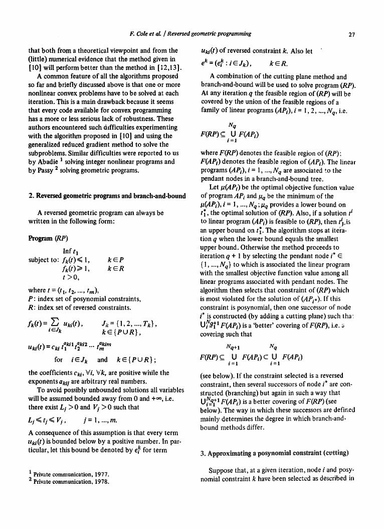
This constraint will be fully characterized by a so- called generating vector gk = (g~ : I E Jk) having the following properties

(i) dim(g k) = Tk, the number of terms in reversed constraint k;

(ii) g~ > 0 , l E J k ;

(iii) ~ g~ < 1. l ~ J k

Hence, a set of generating vectors ~ : k ~ R) together with the cuts already introduced for the posynomial constraints, completely defines a linear program of the branch-and-bound tree. Before dis- cussing how successor nodes of node i are derived, is first showll how the approximating one-term pol~' nomial constraint is obtained from a given generating vector gk. Therefore, define the polyhedron S(g k) as:

This section is a brief review of the theory con- tained in [10] where proofs of the theorems recalled here can be found.

Suppose now that, at a given iteration, node i and reversed constraint k have been selected as described in Section 2. The number of successors of node i will equal the number of terms ukt(t) in reversed con- straint k. We now discuss how these successors are characterized.

In any linear program of the branch-and-bound tree a reversed constraint is represented by exactly

S(gk) = { (Xl : l E Jk) [ Xl >~ gkl , I E J k and ~ x / = 1} Jk

and the set C(g g) as:

C(gk) = { (xl " l ~ Jk) I xt >t x; ,

1E ark, for some (x~ : 1E ark) E S(gk)}.

A generating vector gk and the sets S(g g) and C(g k) are illustrated in Fig. 2 for a reversed con:;traint with two terms.

The exponents at, 1 E JR, and the coefficient ~3k of

(o.1)

i

g ( (~.o)

(o.I~

t l .o)

Fig. 2. Generating vector gk and its associated sets Sfg k) and C~k).

i/¸¸: ii

) ,

Z 1

30 F. Cole et al. / Reversed geometric programming

%

{o.~) T

!

i

,,

a~ 1 11,01

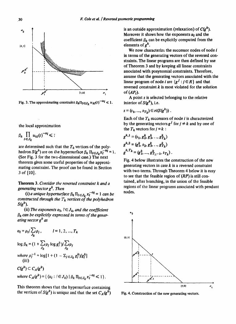
Fig. 3, The approximating constraint fJkHl~__jk ukl(t) -at < 1.

the local approximation

~ I-I uk~(t) - ~ < i t ~Jk

are determined such that the Tk vertices of the poly- hedron S(g k) are on the hypersurface/3k Ht~jkx[ -°~t = 1. (See Fig. 3 for the two-dimensional case.) The next theorem gives some useful properties of the approxi- mating constraint. The proof can be found in Section 3 o f [10].

Theorem 3. Consider the reversed constraint k and a generating vector gk. Then

(j) a unique hypersurface {3 k fit ~Ik xi-at = 1 can be constructed through the Tk vertices o f the polyheclron s(~).

(ii) The exponents at, !, ~ Jk, and the coefficient {3 k can be explicitly expressed in terms o f the gener- ating vector gk as

is an outside approximation (relaxation) of C(g~. Moreover it shows how the exponents 0q and the coefficient/~k can be explicitly computed from the elements o fg k.

We now charaeteriz~ the successor nodes of node i in terms of the generating vectors of the reversed con- straints. The linear programs are then defined by use of Theorem 3 and by keeping all linear constraints associated with posynomial constraints. Therefore, assume that the generating vectors associated with the linear program of node i are {gi .] E R } and that reversed constraint k is most violated for the solution of (APi).

A point s is selected belonging to the relative interior of S(gk), i.e.

s = (s 1 .... , STk ) E ri(S(gk)).

Each of the Tk successors of node i is characterized by the generating vectorsg / for] .~ k and by one of the Tk vectors for ] -- k "

gk., = (Sl, g~. g~, ..... g L )

k, Tk .... gk g -. (gk, Tfr 1, STk)"

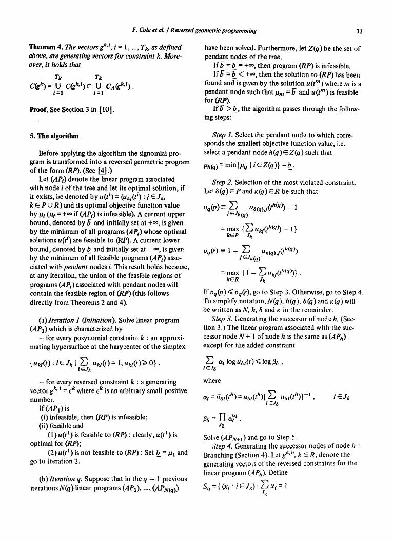
Fig. 4 below illustrates the construction of the new generating vectors in case k is a reversed constraint with two terms. Through Theorem 4 below it is easy to see that the feasible region of (RP) is still con- tained, after branching, in the union of the feasible regions of the linear programs associated with pendant nodes.

~ 2

Otl = P l / ~ P ] , l = 1 ,2 , ..., Tk ~k

log ~ = (1 + ~Jk p~ log g~'. )/._~PJ where.q~ - log[l + (: - ~j~j~g~)/g~]

(iii)

c ~ k) c CA ~k)

where Ca (gk) = { (xt " f E lk ) I {3k flleJk X[ -at <: 1 }.

This theorem shows that the hypersurface containing the vertices of S(g k) is unique and that the set Ca(g k)

(Off)

\ :

(to)

Fig. 4. Construction of the new generating vectors.

• t

av 1

F. Cole et al. / Reversed geometric programming 31

Theorem 4. The vectors gk, i, i = 1, ..., Tk, as defined above, are generating vectors for constraint k. More- over, it holds that

Tk Tk cg ) = U cgS',*)c U CA gk'*).

i " 1 i = 1

Proof. See Section 3 in [I0].

have been solved. Furthermore, let Z(q)be the set of pendant nodes of the tree.

If b = b__ = + % then program (RP) is infeasible. If b = b_ < +0% then the solution to (RP) has been

found and is given by the solution u(t m) where m is a pendant node such that #m = b- and u(t m) is feasible for (R_P).

I f b > b_, the algorithm passes through the follow- ing steps:

5. T h e algorithm

Before applying the algorithm the signomial pro- gram is transformed into a reversed geometric program of the form (RP). (See [4].)

Let (APi) denote the linear program associated with node i of the tree and let its optimal solution, if it exists, be denoted by u(t i) = (ukj(ti) " ] E Jk, k E P U R) and its optimal objective function value by/ai (/ai = +o, if (APi)is infeasible). A current upper bound, denoted by b and initially set at +0% is given by the minimum of all programs (APi) whose optimal solutions u(t i) are feasible to (RP). A current lower bound, denoted by b_ and initially set at _0% is given by the minimum of all feasible programs (APe) asso- ciated with pendant nodes L This result holds because, at any iteration, the union of the feasible regions of programs (APi) associated with pendant nodes will contain the feasible region of (RP)(this follows directly from Theorems 2 and 4).

(a) Iteration 1 (Initiation). Solve linear program (API) which is characterized by

- for every posynomial constraint k : an approxi- mating hypersurface at the barycenter of the simplex

(Uktq)" lEJk l ~ uu(t)= l,uktq)>~O} . t ~Yk

- for every reversed constraint k • a generating vector gk, l = ek where e k is an arbitrary small positive number.

If (API) is (i) infeasible, then (RP) is infeasible;

(ii) feasible and (I) u(t 1) is feasible to (RP) " clearly, u(t 1) is

optimal for (RP); (2) u(t t) is not feasible to (RP)" Set b_ =/al and

go to Iteration 2.

(b) Iteration q. Suppose that in the q - 1 previous iterations N(q) linear programs (AP1), ..., (APN(q))

Step 1. Select the pendant node to which corre- sponds the smallest objective function value, i.e. select a pendam node h(q)E Z(q) such that

Pn(q) = min(Uq l i E Z(q)} =b_.

Step 2. Selection of the most violated constraint. Let 6(q)E P and K(q)ER be such that

] qkJ6 (q )

= max { ~ uki(t ~(q)) - 1 } k~e Jk

Oq(r) -- l -- ~ UK(q),i(t h(q)) J ~-JK(q)

=max - ukj(th 'O)). k E R Jk

If Vq(p) <. Vq(r), go to Step 3. Otherwise, go to Step 4. Fo simplify notation, N(q), h(q), 6(q) and ~:(q) will be written as N, h, 6 and K in the remainder.

Step 3. Generating the successor of node h. (Sec- tion 3.) The linear program associated with the suc- cessor node N + 1 of node h is the same as (APa) except for the added constraint

olt log uu(t) < log/3~ , I EJ6

where

-- a s t ( 3 ) - u6t ( / ' ) [ u l(3)] - l , t ~J6

/~6-- l-] t ~ t . J8

Solve (APN+I) and go to Step 5. Step 4. Generating the successor nodes of node h :

Branching (Section 4). Let gk, a, k E R, denote the generating vectors of the reversed constraints for the linear program (APh). Define

SK

32 F. Cole et al. / Reversed geometric programming

and

Xi>~g~:'h+(1 -- ~ g~'h)M-l , iE]~:)

where M is a constant satisfying M >f maxkE E (Tk).

It is easy to show that Sq ~ 0 and that Sq C riS(gK'h). Select s q = (fit" ] E JK) E Sq. (Notice that the selection of the point s q is slightly more restricted than the procedure described in Section 4. Here s q is restricted to a closed subset of the relative interior of S(g K'n) which is important for the convergence proof of the algorittun. A possible choice for s q is the bary- center of S(g K'h) which always belongs to Sq and which was always used in the computational experi- ments reported on below.)

A total of TK successors (APN+i), i = 1,2, ..., TK, are defined where (APN+i) has generating vectors

gk, N+i =g~,h for k ~ . R - {K}

= . . . . . sO",, 4 , . . . . ,

Linear programs (APN+i), i = 1 .... , TK, are completely characterized by keeping the constraints of (APt,) associated with posynomial constraints and by con- structing the local approximations 'to the reversed constraints form the generating vectors above.

Solve programs (APN+i), i = 1, ..., TK. Step 5. Adjust b__ and b "b__ is the smallest objective

function value over all pendant nodes while b is the smallest objective function value over all pendant nodes with solutions that are feasible for (RP).

If b_ = b, the solution to (RP) is attained and given by the solution u(t m) where m is a pendant node such that ttm = b" and u(t m) is feasible for (RP).

If b_ < b, set q = q + 1 and return.

6. Convergence

It is shown that the algorithm will identify a global minimum to (RP) either in a finite number of steps or as the limit of a converging sub sequence generated by the branch-and-bound tree.

Lemma. A t every iteration q, it holds that

min ~i ~</a , i~Z(q)

where ta* is the minimum o f the oeiginal program (RP).

Proof. This follows directly from Theorem 2(i) and Theorem 4.

Theorem 5. I f the algorithm (i) terminates in a.finite number o f iterations q,

then t~ * = K = b. A solution u* to (RP) is given by m

the solution (APm), m E Z(q), where m is such that am = G and u(t m) is feasible to (RP);

(ii) generates an infinite sequence o f nodes, then every converging subsequenee o f points u(t i) o f an infinite path in the tree converges to an optimal solu- tion ol' (RP).

Proof. (i) By Lemma 2 and the definition of 5, it holds at every iteration that

b < / t * < b .

Since the algorithm terminates in a finite number of steps, it holds at the last iteration that b_ = b" and hence,

ta* =K.

(Notice that b" = +,o implies that (RP) is infeasible.) (ii) Let S be a subsequence of nodes of a path in

the tree such that

lim u(t/) and lim /ai iE8 iE8

exist. Consider a subsequence S ' of S such that con- straint k, k E P U R, has always been used to generate the.successor node(s) of node L i E S '. Because of the lemma it is sufficient to show that

lim u(t/) = u(t**) is feasible for (RP). i ES'

Two cases have to be considered: Case 1. (k E P). First, it is shown that u(t**) satin-

ties constraint k, or that

u ,i(t ®) <<. 1. j ~,rk

Let i and i ' be two successive nodes in S'. Since cuts are never dropped and since i and i ' are on a path, the solution u(t v) satisfies the approximating constraint introduced at node i:

uM(t/) log Ukj(t v)

7 L/eJk l

Letting i, i ' ~ +o% it follows that

ukj(t log( ukj(t')) -<. o j e]k i ~,rk

F. Cole et al. / Reversed geometric programming 33

which implies that

uk/(t**) < l . / ~Jk

It follows easily that u(t**) also satisfies the remaining constraints since otherwise constraint k could never have been selected an infinite number of times along the path.

Case 2. (k E R ) . The proof of this case is more involved but is completely similar to the proof in [ 10].

7. S o m e computat iona l results

An experimental code has been written for this algorithm and some initial results are reported below. The degree of feasibilfty, either 0.01 or 0.003 means that all constraints, when the problem is transformed in the form (RP), are feasible within those bounds. Constraints consisting of one term, ukl (t) - 1, are not included in the number of constraints indicated since they are linear after the logarithmic transforma- tion. We do not report the execution times because of the experimental nature of this code which can be drastically improved, for instance by using post-opti- rrdzation techniques to solve the successor(s) of a node.

Problem 1 (Source [8].)

Min t ] + 2t~ - t l t2

subject to t i t2 ~< 1 9t~ t - 4 t~ l t2 <~ 2 O . l < t l , t 2 < l O .

Number of variables in (RP) form : 5 Number of posynomial constraints : 1 Number of reversed constraints : 2. Feasible within 0.01 : - 29 L.P. problems solved

- t t = 0.503 ; t 2 = 1.989 ; O.F. = 7 . 1 1 .

Feasible within 0.003 : - 3 3 L.P. problems solved

- r I =0.501 ; t2 = 1.997 ; O.F. = 7 .207 .

The optimal solution of this problem is clearly

t I = 0.5 , t2 = 2 , O.F. = 7 .25 .

Problem 2 (Source [ 1 1 ].)

Min 4t~ - t ] - 12

subject to t~ + tzz = 25 10tl - t~ + 1 0 t 2 - t] >I 34 ti >10 .

Number of variables in (RP) form • 5 Number of posynomial constraints • 3 Number of reversed constraints • 3. Feasible within 0.01 • - 3 5 L.P. problems solved.

- t l = 0.90494 ; t2 = 4.91746 ; O.F. = - 3 3 . 0 4 8 4 5 5 .

Feasible within 0.003 • - 4 6 L.P. problems solved.

- t~ = 0.996516 ; t2 = 4 .901 . O.F. = - 3 2 . 1 7 6 3 7 8 .

Problem 3 (Source [2].)

Min(t I - 2)2 + 02 - 1)2

subject to t l - 2t2 + 1 = 0 -0 .25 t21- t22 + 11> 0 ti > t 0 .

Number of variables in (RP) form : 4 Number of reversed constraints : 3 . Feasible within 0.01 : - o 3 L.P. problems solved

- t l = 0.8303 ; t2 = 0.9112 ; O.F. = 1 .28674.

Feasible within 0.003 : - 2 1 1 L.P. problems solved

- t l =0 .8220 ; t2 = 0 . 9 1 1 4 ; O.F. = 1 .374425.

Problem 4 (Source [ 1 4] .)

Min t~ t 2 t3t 4

subject to 4t l ° 's + t~t 3 ~ 1 0.0625t~ 2 + 0.5tl t2 t~ -1 <~ 1 tit222 + 0.25t]r~ < 1 ti 1>0.

The solution given by Reklaitis for this problem is

t I = 0.0625 ; t2 = 8V/-2 ; t3 = 0.5 ; t4 = 2x/~ ; O.F. = 1.

3 4 F. Cole et al. / Reversed geometric programming

However, it can easily be seen that this is not the global situation to the p,'oblem. Indeed by consider-

ing the point

t 1 = n-1., t2 = t3 = t 4 = 1

and letting n -~ +*% it follows immediately that the infimum of this problem is zero. Although this algo- rithm and its convergence was written for bounded problems, the unbounded nature of the solution (characterized in geometric programming by the fact that there is no optimal solution of the problem with t > O) is clearly hinted a" by the approximating solu- tions produced by our code.

S.t.:

C I3X2X $ + C14X l X 2 "k C15X23 CI6X'~Ix '~ 1 .- C17XIX~ 1 -- C l8X4X~ 1

C I g X a X s - - C 2 0 X I X 3 + C21XaX 4

78 ~<x I ~< 102 33 ~<x2 < 45

2 7 < x a < 45 27 ~<x 4 ~< 4 5 27~<Xs ~< 45

c4xax s - CsX2X s - C6XlX 4 ~ 1 C7X2X5 + t ? 8 X I X 4 - - C9X3X 5 '<~ 1 CIox~lx-~I e11XlX.~1 --1 2 --1 .~ 1 . . . . e 1 2 x 2 x a x s

<~1 < 1 < 1

i ei i ei

Number of variables in (RP) form • 5 Number of posynomial constraints • 2 Numb6r of reversed constraints • 1. Feasible within 0.01 • - 5 L.P. problems solved

- t~ =0•9357762 D-13 ; t2 = 44.7917 ; ta = 4.03272 ; t4 = 0.209572 D-11 ; O.F. = 0.354237 D - 2 2 .

Feasible within 0.003 " - 6 L.P. problems solved

- t~ = 0•935762 D-13 ; tz --34•867 ; t3 = 6•655522 ; t4 -- 0.16136 D-11 ; O.F. -- 0.3.54237 D - 2 2 .

¢

]Problem 5 (Source [3].)

Min 0.4t 0"67t~ "0"67 + 0.4t20"67t~ °'67 - tl - t2 + 10

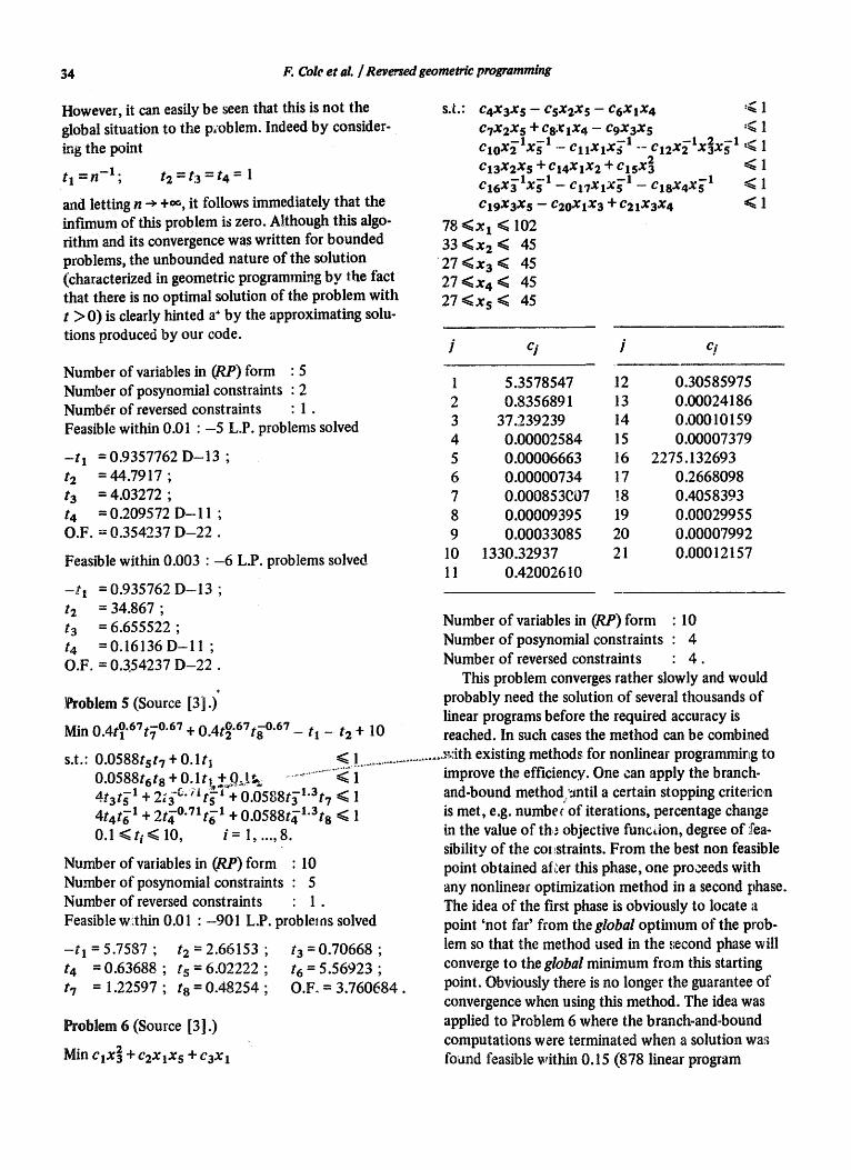
1 5•3578547 12 0.30585975 2 0.8356891 13 0.00024186 3 37.239239 14 0•00010159 4 0.00002584 15 0•00007379 5 0.00006663 16 2275.132693 6 0•00000734 17 0.2668098 7 0.000853C07 !8 0.4058393 8 0.00009395 19 0.00029955 9 0.00033085 20 0.00007992

10 1330.32937 21 0.00012157 11 0.42002610

Number of variables in (RP) form : 10 Number of posynomial constraints : 4 Number of reversed constraints : 4 .

This problem converges rather slowly and would probably need the solution of several thousands of linear programs before the required accuracy is reached. In such eases the method can be combined

• 0 0588t t + 0 1 t~ < 1 .g:ith existing methods for nonlinear programming to s.t. . s 7 • ............................. 0 0588t t + 0 It) + 0 1 ,,, ................... <" 1 improve the efficiency• One can apply the branch- . 6 8 • ~.~, ~,~ - 4tat~ 1 + 213 - c '~ t s l + 0.O588t~l"at7 < 1 and-bound method.'~ntil a certain stopping criteric,n 4t4t~ 1 + 2t~ "°'71tg -1 + 0.0588t~-L3ts < 1 is met, e.g. numbec of iterations, percentage change

0.1 <~ti<<. 10, i = 1, ...,8.

Number of variables in (RP)form • 10 Number of posynomial constraints • 5 Number of reversed constraints • I . Feasible within 0.01 • -901 L.P. proble~ns solved

- t 1=5 .7587 ; t2 =2 .66153; t4 = 0•63688 ; ts = 6.02222 ; t 7 = 1•22597 ; ta =0•48254 ;

ta = 0.70668 ; t 6 = 5.56923 ; O.F, = 3.760684•

Problem 6 (Source [3].)

Min Cl x2 + c2x~xs + C3Xl

in the value of th,. • objective function, degree of fea- sibility of the col~straints. From the best non feasible point obtained after this phase, one pro~.eeds with any nonlinear optimization method in a second phase. The idea of the first phase is obviously to locate a point 'not far' from the global optimum of the prob- lem so that the method used in the ,.;econd phase will converge to the global minimum from this starting point. Obviously there is no longer the guarantee of convergence when using this method. The idea was applied to Problem 6 where the branch-and-bound computations were terminated when a solution was found feasible within 0.15 (878 linear program

F. Cole et ai. / Reversed geometric programming 35

solved). This produced the solution

x l = 78.00 x2 = 33.00 xa = 29.5917 x4 = 45.00 Xs = 27.00 O.F. = 9356.32768

(lower b o u n d ) .

The generalized reduced gradient method was then used starting from this point and produced the solu- tion below in three more iterations:

x l = 78.00 x2 = 33.00 xa = 29.996 x4 = 45.00 Xs = 36.774 O.F. = 10 122.69 .

This solution agrees with the solution obtained in [3] and is likely the global minimum of the problem.

References

[ 1 ] M. Avriel, R. Dembo and U. Passy, Solution of generab ized geometric programs, Intemat. J. Numer. Methods Engrg. 9 0975).

[2] J. Bracken and G.P. McCormick, Selected Applications of Nonlinear Programming (Wiley, New York, 1968).

[ 3 ] R. Dembo, A set of geometric programming test prob- lems and their solutions, Working Paper 87, Department of Management Sciences, University of Waterloo (1974).

[4 ] R. Duff'm and E. Peterson, Geometric programming with signomials, J. Optimization Theory Appl. 11 (1) (1973).

[51

[61

[7l

[81

[9l

[lO]

[ l l l

i12l

[13l

ll4l

[151

C. Eaves and W. Zangwi.~l, Generalized cutting plane algorithms, SIAM J. Control 9 (1971). J. Ecker and M. Zoracki, An easy primal method for geometric programming, Management Sci. 23 (1) (1976). J. Falk and R. Soland, An algorithm for separable nonconvex programming problems, Management Sci. 15 (1969). J. Falk, Global solutions of signomial programs, Serial T-274, The George Washington University (1973). W. Gochet and Y. Smeers, On the use of linear programs to solve prototype geometric programs, Cahiers Centre Etudes Recherche Op6r. 16 (1) (1974). W. Gochet and Y. Smeers, A branch-and-bound method for reversed geometric programming, CORE Discussion Paper 7511, Catholic University (3f Louvain (1975). To appear in Operations Res. D. Himmelbl~u, Applied Nonlinear Programming (McGraw-Hill • New York, 1972). U. Passy, Sign omial geometric programming: Determin- ing the global minimum, in: P. Van Moeseke (ed.), Ma- thematical Pr,~grams for Activity Analysis (North-Hol- land, Amster~ am, 1974). U. Passy, Glo')al solutions of mathematical programs with intrinsically concave functions, J. Optimization Theory Appl. 26 (1) (1978). G.V. Reklaiti~, The underlying primal structure and its use in computation, in: Philips and Beightler (eds.), Applied Geometric Programming (Wiley, New York, 1976). Y. Smeers, Studies in geometric programming with applications to management science, Ph.D. Thesis, Carnegie-Mellon University (1972).