Reverse Mortgage Loans: A Quantitative Analysis - · PDF fileReverse Mortgage Loans: A Quantitative Analysis Makoto Nakajimay Federal Reserve Bank of Philadelphia Irina A. Telyukovaz

Reverse Mortgage Loans:A Quantitative Analysis∗

Makoto Nakajima†

Federal Reserve Bank of PhiladelphiaIrina A. Telyukova‡

University of California, San Diego

April 1, 2013

Abstract

Reverse mortgages allow elderly homeowners with limited income or financial wealth to bor-row against their housing wealth without downsizing or moving out and becoming a renter.Although the proportion of eligible older homeowners using reverse mortgages has been increas-ing rapidly, that proportion is only 1.4 percent at present. In this paper, we analyze reversemortgage loans in a rich structural life-cycle model of retirement. Our model can replicate thelow take-up rate with a reasonable calibration. When the model is calibrated to match the ob-served take-up rate, the welfare gain from introducing reverse mortgages is sizable at $510 perhousehold in the economy. Our model indicates that one-third of reverse mortgage borrowersuse them for medical expenses, while remaining in their home. Through counterfactual exper-iments, we identify that, conditional on the existing RML contracts, bequest motives, movingshocks, and house price fluctuations all contribute to the observed low take-up rate, and thatif households expect a housing boom, reverse mortgage demand increases, consistent with thedata. However, the interest and insurance costs of reverse mortgages are important deter-minants of demand as well. Finally, the addition of the HECM Saver, a recently-introducedreverse mortgage contract with lower upfront costs designed to boost demand for reverse mort-gages, fails to create that boost.

JEL classification: D91, E21, G21, J14Keywords: Reverse Mortgage, Mortgage, Housing, Retirement, Home Equity ConversionMortgage, HECM

∗We thank the participants of the 2011 SAET Meetings in Faro, and 2011 SED Meetings in Ghent, for theirfeedback. The views expressed here are those of the authors and do not necessarily represent the views of the FederalReserve Bank of Philadelphia or the Federal Reserve System.†Research Department, Federal Reserve Bank of Philadelphia. Ten Independence Mall, Philadelphia, PA 19106-

1574. E-mail: [email protected].‡Department of Economics, University of California, San Diego. 9500 Gilman Drive, San Diego, CA 92093-0508.

E-mail: [email protected].

1

1 Introduction

Reverse mortgage loans (RMLs) allow elderly homeowners to borrow against their housing wealthwithout moving out of the house, while insuring them against significant drops in house prices.Despite potentially large benefits to older individuals, many of whom want to stay in their houseas long as possible, frequent coverage in the media, and the attempts by the Federal HousingAdministration which administers RMLs to change the contract to make it more appealing toborrowers, little research has been done on reverse mortgages. This paper is intended to fill thevoid.

In previous work, Nakajima and Telyukova (2012) find that elderly homeowners become severelyborrowing-constrained as they age, as it becomes very costly to access their home equity, and thatthese constraints force many homeowners to sell their homes, when faced with large expense shocks.In this environment, it seems that an equity borrowing product targeted toward the elderly wouldbe able to relax that constraint, and hence benefit many homeowners. Empirical studies havecome to similar conclusions. For example, Rasmussen et al. (1995) argue, using 1990 U.S. Censusdata, that almost 80 percent of homeowner households of age 69 or above should benefit fromreverse mortgages. Using a more conservative approach, Merrill et al. (1994) find that about 9percent of homeowner households over age 69 could benefit from reverse mortgage loans.1 Despitethe apparent benefits, only about 1.4 percent of elderly homeowners were using reverse mortgagesin 2009, although this represents the highest level of demand to date, as the take-up of reversemortgages increased dramatically between 2000 and 2009.

In this paper, we want to answer three key questions about reverse mortgages. First, we want tounderstand who benefits from reverse mortgages, and how large are welfare gains from introducingRMLs. Second, we ask, given the current available RML contract, what prevents retirees fromtaking the loans more frequently. Here we focus on retirees’ environment, such as the nature ofuncertainty that they face, and motivations, such as their bequest motives, which in previous workwe established to be strong. Third, we want to understand what about the nature of the contractitself may prevent retirees from borrowing, and how this contract can be changed to make theRML more beneficial to retirees and this increase the take-up rate. We are motivated here by thefrequently-advanced argument that the low take-up rate in the data is due to the high upfront feesof RMLs.

To answer these questions, we use a rich structural model of housing and saving/borrowingdecisions in retirement based on Nakajima and Telyukova (2012), and study reverse mortgage loansthrough the lens of this model. In the model, households are able to choose between homeownershipand renting, and homeowners can choose at any point to sell their house or to borrow againsttheir home equity. Retirees face uncertainty in their life span, health, medical expenses, and houseprices. The model is estimated to match life-cycle profiles of net worth, housing and financial assets,homeownership rate, and home equity debt. Into this model, we introduce reverse mortgages, tounderstand who takes RMLs and to quantify welfare gains to different types of households, and

1Rasmussen et al. (1995) assume that elderly households with home equity exceeding $30,000 and withoutmortgage loans in 1990 benefit from having the option of obtaining reverse mortgage loans. Merrill et al. (1994)assume that households with housing equity between $100,000 and $200,000, income of less than $30,000 per yearand strong commitment to stay in the current house (specifically those who have no moved for the last 10 years) andwho own their house free and clear benefit from reverse mortgages.

2

then conduct counterfactual experiments to answer the questions we posed above.

There are five key findings. First, the model can replicate the observed low take-up rate (1.4percent) with a reasonable calibration. The households who use reverse mortgages tend to be low-income, low-wealth and poor-health households. Second, the ex-ante expected welfare gain fromintroducing RMLs into a world where they do not exist is sizable – equivalent to 510 dollars ofone-time transfer for all households at age 65. Third, our model indicates that one-third of RMLborrowers use reverse mortgages to pay for medical expenses while allowing them to remain in theirhome, where the alternative in the world without RMLs would have been to sell the house. Fourth,through counterfactual experiments, we identify that bequest motives, moving shocks, and houseprice fluctuations are the features of the environment that particularly discourage the elderly fromusing RMLs. Episodes of housing price booms, like the most recent one, can also boost demand forRMLs which parallels the boost we observe in the data. We also find that eliminating some of theseenvironment features changes the dominant reasons for why homeowners take up RMLs; withoutbequest motives, for example, retirees not only take RMLs much more frequently, but also use themoverwhelmingly for non-medical consumption. Fifth, on the contract side, we find that reducingflow costs of insurance against house price drops increases demand for RMLs. Strikingly, we findthat retirees do not value the insurance component of RMLs, due to low borrowed amounts andavailability of government-provided programs such as Medicaid, so that eliminating altogether thisinsurance against house price fluctuation increases RML demand by 43 percent. Thus, the oft-heardclaim that large contract costs suppress RML demand is supported by our model. However, theHECM Saver loan, which was designed to respond to this claim by lowering the upfront cost ofinsurance in exchange for lowering the amount of equity accessible to the elderly, reduces demandfor reverse mortgages in our model, so that adding it to already existing RML contracts is not likelyto boost demand.

Our paper is related to four branches of the literature. First, the literature on reverse mortgageloans is developing, reflecting the growth of the take-up rate and the aging population. Shan(2011) empirically investigates the characteristics of reverse mortgage borrowers. Redfoot et al.(2007) explore better design of reverse mortgage loans by interviewing reverse mortgage borrowersand those who considered reverse mortgages, but eventually decided not to utilize them. Davidoff(2012) investigates under what conditions reverse mortgages may be beneficial to homeowners, butin an environment where many of the idiosyncratic risks that we model are absent. Michelangeli(2010) is closest to our paper in approach. She uses a structural model with moving shocks andfinds that, in spite of the benefits, many households would suffer from using reverse mortgagesbecause of involuntary moving shocks. Our model can provide more realistic estimates of the shareof beneficiaries of reverse mortgages, and the size of their welfare gains, by modeling various kinds ofshocks that elderly households face, such as health status, medical expenditures, moving, and priceof their house. Moreover, by taking the initial type distribution of elderly households from the data,our model can also predict the take-up rate and what types of households benefit from availabilityof reverse mortgage loans. Finally, we model the popular option of a line of credit reverse mortgageloan, while she assumes that borrowers have to borrow the maximum amount at the time of theclosing. We find that this distinction in the form of the contract matters.

The second relevant strand of literature addresses saving motives for the elderly, or solving theso-called “retirement saving puzzle.” Hurd (1989) estimates the life-cycle model with mortalityrisk and bequest motives and finds that the intended bequests are small. Ameriks et al. (2011)

3

estimate the relative strength of the bequest motives and public care aversion, and find that thedata imply both are significant. De Nardi et al. (2010) estimate in detail out-of-pocket (OOP)medical expenditure shocks using the Health and Retirement Study, and find that large OOPmedical expenditure shocks are the main driving force for retirement saving, to the effect thatbequest motives no longer matter. Venti and Wise (2004) study how elderly households reducehome equity. In out previous work, Nakajima and Telyukova (2012) emphasize the role of housingand collateralized borrowing in shaping the retirement saving, and find that bequest motives andhomeownership motives are key in accounting for the retirement saving puzzle, in addition to medicalexpense uncertainty.

Third is the literature on mortgage choice, in particular, using structural models, which isgrowing in parallel with developments in the mortgage markets. Chambers et al. (2009b) constructa general equilibrium model with a focus on the optimal choice between conventional fixed-ratemortgages and newer mortgages with alternative repayment schedules. Campbell and Cocco (2003)investigate the optimal choice for homebuyers between conventional fixed-rate mortgages (FRM)and more recent adjustable-rate mortgages (ARM). We model the choice between conventionalmortgages and line-of-credit reverse mortgages, though we focus only on retirees.

Finally, since one of the characteristics of the reverse mortgage loans is the availability of thetenure option, which is equivalent to annuitizing one’s house, the paper is related to the “annuitypuzzle” literature, although we do not treat the tenure option explicitly, since it is not prevalent inthe data. Since the seminal work by Yaari (1965), many explanations for the low demand of annuitiesare proposed. Dushi and Webb (2004) argue that individuals already have significant amount ofannuitized wealth in the form of Social Security and Defined Benefits pension plans. Mitchell et al.(1999) find that annuity prices are too high compared with actuarially fair prices in the U.S. data.Lockwood (forthcoming) find importance of bequest motives and the inability of annuitized wealthto be bequeathed. Turra and Mitchell (2004) study the role of medical expenditure risks. A recentpaper by Pashchenko (2004) investigates the relative importance of the existing explanations of theannuity puzzle.

The remainder of the paper is organized as follows. Section 2 provides an overview of the reversemortgages. Section 3 develops the structural model that we use for experiments. Section 4 discussesthe calibration of the model. In Section 5, we use the model to analyze the demand for reversemortgages through a number of counterfactual experiments. Section 6 concludes.

2 Reverse Mortgage Loans: An Overview

Currently, the most popular type of reverse mortgage is administered by the government, while theprivate market for reverse mortgages has been shrinking.2 The government-administered reversemortgage is called a home equity conversion mortgage (HECM). These mortgage loans are admin-istered by the Federal Housing Administration (FHA), which is part of the U.S. Department ofHousing and Urban Development (HUD). According to Shan (2011), HECM loans represent over90 percent of all reverse mortgages originated in the U.S. market.3

2This section is based on, among others, AARP (2010), Shan (2011), Nakajima (2012), and information availableon the HUD website.

3Many other reverse mortgage products, such as Home Keeper mortgages, which were offered by Fannie Mae, orthe Cash Account Plan offered by Financial Freedom, were recently discontinued, in parallel with the expansion ofthe HECM market. See Foote (2010).

4

0

0.3

0.6

0.9

1.2

1.5

1997 1999 2001 2003 2005 2007 2009

Year

Figure 1: Percentage of Elderly (age≥65) Homeowners with Reverse Mortgages.Source: American Housing Survey, Various Waves.

The number of households with reverse mortgages is growing rapidly. Figure 1 shows the pro-portion of homeowner households of age 65 or above that had reverse mortgages between 1987 and2009. Both the government-administered HECM loans and private mortgage loans are included.As the figure shows, the use of reverse mortgages was limited before 2000. In 2001, the share ofeligible homeowners who had reverse mortgages was about 0.2 percent. This share increased rapidlysince then, reaching 1.3 percent in 2009. Although the level is still low, the growth is all the moreimpressive if one considers that the popularity of reverse mortgages continued to rise even thoughthe housing market and mortgage markets in general have been stagnating since the beginning ofthe ongoing housing market downturn.

Reverse mortgages differ from conventional mortgages in six major ways. First, as the namesuggests, a reverse mortgage loan works in the reverse way from the conventional mortgage loan.Instead of paying interest and principal and accumulating home equity, reverse mortgage loans allowhomeowners to cash out the home equity they’ve accumulated. That is why RMLs are targeted toolder households.

Second, government-administered reverse mortgages (HECM loans) have different requirementsthan conventional mortgage loans. These mortgages are available only to borrowers age 62 or older,who are homeowners and live in their house.4,5 Finally, borrowers must have repaid all or almost allof their other mortgages at the time they take out a reverse mortgage. On the other hand, reversemortgage loans do not have income or credit history requirements, because repayment is promisednot based on the borrower’s income but solely on the value of the house the borrower already owns.According to Caplin (2002), reverse mortgage loans are beneficial for elderly homeowners since

4For a household with multiple adults who co-borrow, “age of the borrower” refers to the youngest borrower inthe household.

5Properties eligible for HECM loans are (1) single-family homes, (2) one unit of a one- to four-unit home, and(3) a condominium approved by HUD.

5

many of them fail to qualify for conventional mortgage loans because of income requirements.

Third, reverse mortgage borrowers are required to seek counseling from a HUD-approved coun-selor in order to be eligible for a HECM loan. The goal is to be certain that older borrowersunderstand what kind of loan they are getting and what the potential alternatives are before takingout a reverse mortgage loan.

Fourth, there is no pre-fixed due date; repayment of the borrowed amount is due only when thehouse is sold and all the borrowers move out, or when all the borrowers die. As long as at leastone of the borrowers continues to live in the same house, there is no need to repay any of the loanamount. There is no gradual repayment with a fixed schedule, as with a conventional mortgageloan or line of credit; repayment is made in a lump sum from the proceeds from the sale of thehouse.

Fifth, HECM loans are non-recourse; borrowers are insured against substantial drops in houseprices. Borrowers (or their heirs) can repay the loan either by letting the reverse mortgage lendersell the house, or by repaying. Most use the first option. If the sale value of the house turns out tobe larger than the sum of the total loan amount and the various costs of the loan, the borrowersreceive the remaining value. In the opposite case, where the house value cannot cover the total costsof the loan, the borrowers are not liable for the remaining amount. The mortgage lender does nothave to absorb the loss either, because the loss is covered by insurance, with the premium includedas a part of a HECM loan cost structure.

Finally, there are various ways to receive payments from the RML. Borrowers can choose one offive options, and these can be changed during the life of the loan, at a small cost. The options are:

• Tenure: Borrowers continue to receive a fixed amount as long as one of the borrowers con-tinues to live in the same house.

• Term: Borrowers receive a fixed amount for a fixed length of time.

• Line of credit: Borrowers can flexibly draw cash, up to a limit, during a pre-determineddrawing period.

• Modified tenure: Combination of the tenure option and the line of credit option.

• Modified term: Combination of the term option and the line of credit option.

Of the payment options listed, the line of credit option has been the most popular. HUD reportsthat the line of credit plan is chosen either alone (68 percent) or in combination with the tenure orterm plan (20 percent). In other words, it appears that older homeowners use reverse mortgagesmainly to flexibly withdraw cash out of accumulated home equity.

How much can one borrow using a reverse mortgage? Let’s start with the case in which borrowersreceive a one-time cash payment under a reverse mortgage. The starting point is the appraised valueof the house, but there is a federal limit for a government-administered HECM loan. Currently, thelimit is 625, 500 dollars for most states.6 The less of the appraised value and the limit is called the

6The limit was raised in 2009 from 417, 000 dollars as part of the Housing and Economic Recovery Act of 2008.The 625, 500 limit is valid until December 2011.

6

0

0.01

0.02

0.03

0.04

0.05

0 10 20 30 40 50 60 70 80 90

Initial Principal Limit as a percentage of house value

Figure 2: Initial Principal Limit Distri-bution. Source: Shan (2011).

0

0.02

0.04

0.06

62 67 72 77 82 87 92 97

Age of borrowers

Figure 3: Age at Reverse MortgageOrigination. Source: Shan (2011).

Maximum Claim Amount (MCA).7 Reverse mortgage borrowers cannot receive the full amount ofthe MCA because there are various costs that have to be paid from the house value as well. Thereare two types of costs: non-interest costs and interest costs. Moreover, if borrowers have outstandingmortgages, part of the new mortgage loan will be used to pay off the outstanding balance of othermortgages. Non-interest costs include an origination fee, closing costs, the insurance premium, anda loan servicing fee. The insurance premium depends on the value of the house and how long theborrowers live and stay in the same house. More specifically, the insurance premium is 2 percentof the appraised value of the house (or the limit if the value is above the limit) initially and 1.25percent of the loan balance annually.8 Interest costs depend on the interest rate, the loan amount,and how long the borrowers live and stay in the house. The interest rate can be either fixed oradjustable. In case of an adjustable interest rate, the borrowing interest rate is the sum of thereference interest rate plus margin charged by the mortgage lender, and there is typically a ceilingon how much the interest rate can go up per year or during the life of a loan. The Initial PrincipalLimit (IPL) is calculated by subtracting expected interest costs from the MCA. The Net PrincipalLimit is calculated by subtracting various upfront costs from the IPL.

The IPL, which is the amount available for reverse mortgage borrowers at the time of closing,is thus larger the larger the house value, the lower the outstanding mortgage balance, the older theborrower, and the lower the interest rate. Figure 2 shows the distribution of the initial principallimit as a percentage of the house value against which mortgage loans are borrowed. It is clearthat many homeowners can borrow around 60 to 70 percent of the appraised house value usingreverse mortgages. If the term option is chosen, the total loan amount is divided depending on thenumber of times the borrower receives cash. With the tenure option, the amount of cash paymentper period is determined by the number of times the borrowers are expected to receive cash.

To understand who the reverse mortgage borrowers are, Shan (2011) looked at the characteristicsof areas with more reverse mortgage borrowers and investigated how those characteristics changed

7Private mortgage lenders offer jumbo reverse mortgage loans, which allow borrowers to cash out more than thefederal limit. However, borrowers have used jumbo reverse mortgages less and less often as the federal limit has beenraised.

8Annual mortgage insurance premium was raised from 0.5 percent to 1.25 percent in October 2010.

7

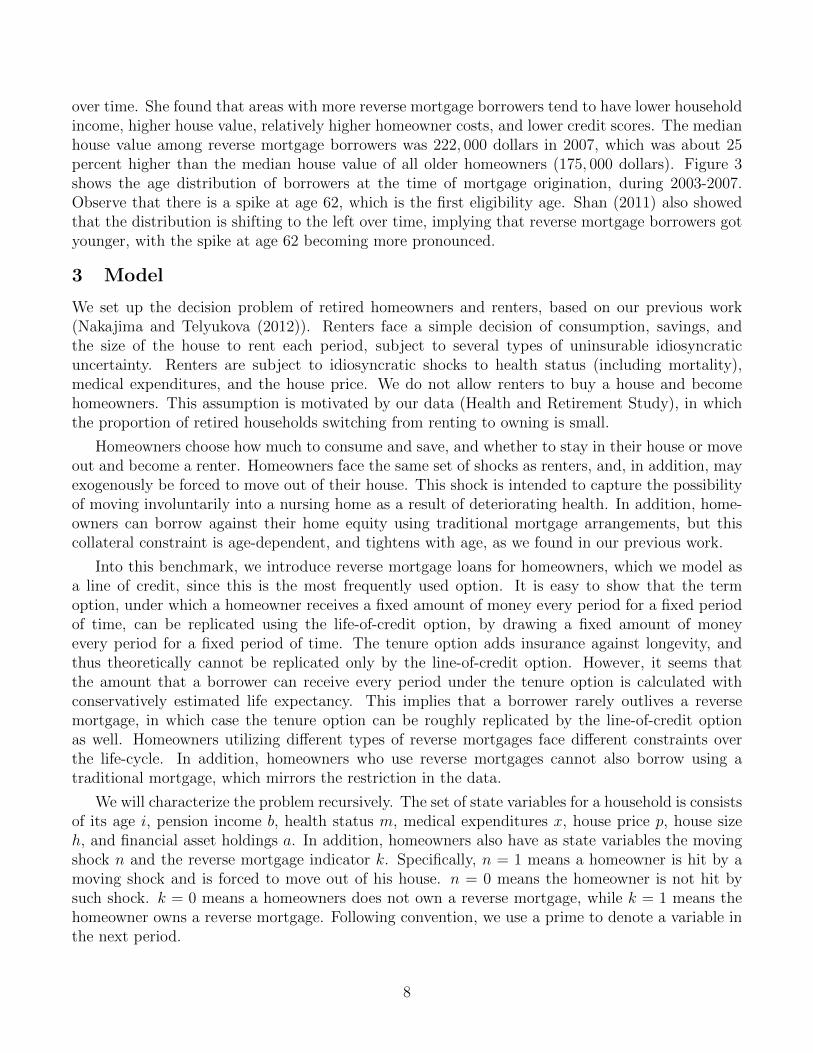
over time. She found that areas with more reverse mortgage borrowers tend to have lower householdincome, higher house value, relatively higher homeowner costs, and lower credit scores. The medianhouse value among reverse mortgage borrowers was 222, 000 dollars in 2007, which was about 25percent higher than the median house value of all older homeowners (175, 000 dollars). Figure 3shows the age distribution of borrowers at the time of mortgage origination, during 2003-2007.Observe that there is a spike at age 62, which is the first eligibility age. Shan (2011) also showedthat the distribution is shifting to the left over time, implying that reverse mortgage borrowers gotyounger, with the spike at age 62 becoming more pronounced.

3 Model

We set up the decision problem of retired homeowners and renters, based on our previous work(Nakajima and Telyukova (2012)). Renters face a simple decision of consumption, savings, andthe size of the house to rent each period, subject to several types of uninsurable idiosyncraticuncertainty. Renters are subject to idiosyncratic shocks to health status (including mortality),medical expenditures, and the house price. We do not allow renters to buy a house and becomehomeowners. This assumption is motivated by our data (Health and Retirement Study), in whichthe proportion of retired households switching from renting to owning is small.

Homeowners choose how much to consume and save, and whether to stay in their house or moveout and become a renter. Homeowners face the same set of shocks as renters, and, in addition, mayexogenously be forced to move out of their house. This shock is intended to capture the possibilityof moving involuntarily into a nursing home as a result of deteriorating health. In addition, home-owners can borrow against their home equity using traditional mortgage arrangements, but thiscollateral constraint is age-dependent, and tightens with age, as we found in our previous work.

Into this benchmark, we introduce reverse mortgage loans for homeowners, which we model asa line of credit, since this is the most frequently used option. It is easy to show that the termoption, under which a homeowner receives a fixed amount of money every period for a fixed periodof time, can be replicated using the life-of-credit option, by drawing a fixed amount of moneyevery period for a fixed period of time. The tenure option adds insurance against longevity, andthus theoretically cannot be replicated only by the line-of-credit option. However, it seems thatthe amount that a borrower can receive every period under the tenure option is calculated withconservatively estimated life expectancy. This implies that a borrower rarely outlives a reversemortgage, in which case the tenure option can be roughly replicated by the line-of-credit optionas well. Homeowners utilizing different types of reverse mortgages face different constraints overthe life-cycle. In addition, homeowners who use reverse mortgages cannot also borrow using atraditional mortgage, which mirrors the restriction in the data.

We will characterize the problem recursively. The set of state variables for a household is consistsof its age i, pension income b, health status m, medical expenditures x, house price p, house sizeh, and financial asset holdings a. In addition, homeowners also have as state variables the movingshock n and the reverse mortgage indicator k. Specifically, n = 1 means a homeowner is hit by amoving shock and is forced to move out of his house. n = 0 means the homeowner is not hit bysuch shock. k = 0 means a homeowners does not own a reverse mortgage, while k = 1 means thehomeowner owns a reverse mortgage. Following convention, we use a prime to denote a variable inthe next period.

8

3.1 Renters

We start with the renter’s decision problem, the simpler of the two household types, since rentingis the absorbing tenure state (remember a renter cannot become a homeowner by assumption). Inorder to save notation, we use h = 0 to represent a renter. h > 0 means that the household is ahomeowner with a house size of h. The renter’s problem is as follows:

V (i, b,m, x, p, k = 0, h = 0, a) = maxh∈H,a′≥0

{u(i, c, h, 0)

+ β∑m′>0

πmi,m,m′

∑x′

πxi+1,m′,b,x′

∑p′

πpp,p′V (i+ 1, b,m′, x′, p′, k = 0, h = 0, a′) + βπmi,m,0v(a′)

}(1)

subject to:

c+ a′ + xχi + rhh = (1 + r)a+ bχi (2)

c =

{max{cχi − rhh, c} if a′ = 0c otherwise

(3)

Naturally a renter has no house (h = 0), and no reverse mortgage (k = 0). A renter, taking thestates as given, chooses consumption (c), savings (a′), and the size of the house to rent (h). (m,x, p)are the shocks. h is chosen from a discrete set H = {h1, h2, ..., hH}, where h1 is the smallest andhH is the largest house available. a′ is assumed to be non-negative. In other words, only homeequity borrowing is available in the model. This choice is motivated by the data, where holdingsof unsecured debt among retirees are small.9 πmi,m,m′ , πxi+1,m′,b,x′ , and πpp,p′ denote the transitionprobabilities of (m,x, p), respectively. m > 0 indicates health levels, with a higher m for betterhealth. The transition of m also includes mortality risk; m′ = 0 implies that the renter does notsurvive to the next period. Note that health shocks are age-dependent, and medical expense shocksdepend on the current health, age and income of the household. Both are motivated by the data.

The current utility of the renter depends on non-housing consumption c, services generated bythe rental property (which are assumed to be linear in the size of the rental property h), and tenurestatus o. Age i in the utility captures the adjustment we make by the age-specific average householdsize factor, which weights utility of couples differently from utility of single households. This factorcaptures the fact that a younger retired household is more likely to be a couple, and we includecouples as well as singles in our data sample.

o = 1 represents ownership, while o = 0 indicates renting. The tenure status in the utilityfunction is intended to capture the additional private value of owned housing. The continuationvalue is discounted by the subjective discount factor β. Following De Nardi (2004), we assumewarm-glow bequest motive with utility function v(a′).

Equation (2) is the budget constraint for a renter. The expenditures on the left-hand side includeconsumption (c), savings (a′), rent payment with the rental rate rh, and medical expenditures x,

9We discuss many of our model assumptions in more detail in Nakajima and Telyukova (2012)

9

which are multiplied by age-specific average household size factor χi discussed above. The right-hand side includes financial asset holdings and interest income (1+r)a and pension income b, againmodified by the age-specific household size factor χi. Equation (3) represents the consumptionfloor, which is provided by the government net of the rental payment. If the sum of c implied in thebudget constraint (2) and the rent payment rhh is lower than the consumption floor (c) multipliedby the age-specific household size factor, the household can consume cχi, net of the rent payment,with the support from the government, if the household runs down its savings (a′ = 0). This modelfeature represents Medicaid in the data.

3.2 Homeowners Without a Reverse Mortgage

First we describe the problem of a homeowner without a reverse mortgage (k = 0). If the homeowneris hit by a moving shock (n = 1), he has to sell the house and move out, i.e. become a renter in thelanguage of the model (V0). Otherwise (n = 0), he can choose whether to stay in the same house(V1), stay in the house and take out a reverse mortgage (V2), or sell the house and become a renter(V0). These two scenarios are represented by the following two expressions:

V (i, b,m, x, p, n = 1, k = 0, h, a) = V0(i, b,m, x, p, k = 0, h, a) (Move out involuntarily) (4)

V (i, b,m, x, p, n = 0, k = 0, h, a) = max

V0(i, b,m, x, p, k = 0, h, a) (Move out)V1(i, b,m, x, p, k = 0, h, a) (Stay)V2(i, b,m, x, p, k = 0, h, a) (Stay, take RML)

(5)

The component value functions are defined below. For an owner with no reverse mortgage, whodecides to move out, or is forced to do so,

V0(i, b,m, x, p, k = 0, h, a) = maxa′≥0

{u(i, c, h, 1)

+ β∑m′>0

πmi,m,m′

∑x′

πxi+1,m′,b,x′

∑p′


}(6)

subject to:

c+ a′ + xχi + δh = (1− κ)hp+ (1 + r)a+ bχi (7)

c =

{max{cχi, c} if a′ = 0c otherwise

(8)

r =

{r + ιm if a < 0r otherwise

(9)

Compared to the problem of the renter, the new features here are that the owner, in the currentperiod, has to pay a maintenance cost δ to keep the house from depreciating, and pay the sellingcost κ. In addition, if the homeowner is in debt at the time of house sale, the interest rate has amortgage premium ιm on it, as defined in (9), but going forward he can no longer borrow. Finally,the consumption floor does not include a rental payment in the current period because the ownerstill lives in his house.

10

The Bellman equation of a homeowner who stays in the house and does not take out a reversemortgage in the next period is

V1(i, b,m, x, p, k = 0, h, a) = maxa′≥(1−λmi )h

{u(i, c, h, 1)

+ β∑m′>0

πmi,m,m′

∑x′

πxi+1,m′,b,x′

∑p′

πpp,p′∑n′

πni+1,m′,n′V (i+ 1, b,m′, x′, p′, n′, k = 0, h, a′)

+ βπmi,m,0∑p′

πpp,p′v((1 − κ)hp′ + a′)

}(10)

subject to:

c+ a′ + xχi + δh = (1 + r)a+ bχi (11)

r =


(12)

The differences from previous equations are that this homeowner can borrow on a traditional mort-gage with the age-dependent collateral constraint λmi , and in the event of death, the estate includesthe value of the house, net of the selling cost to liquidate it (κhp′). In addition, the continuationvalue for this homeowner includes the probability pini+1,m′,n′ of the involuntary moving shock, whichdepends on age and health. It is natural to assume that the involuntary moving shock dependson age and health status since it is intended to capture the incident of involuntary moving intoa nursing home. Finally, as long as the household remains a homeowner, he does not utilize theconsumption floor. In other words, we assume no homestead exemption.10 Next is the problem ofa homeowner who stays in the house and takes out a reverse mortgage going forward:

V2(i, b,m, x, p, k = 0, h, a) = maxa′≥(1−λr)h

{u(i, c, h, 1)

+ β∑m′>0

πmi,m,m′

∑x′

πxi+1,m′,b,x′

∑p′

πpp,p′∑n′


+ βπmi,m,0∑p′

πpp,p′v(max {(1− κ)hp′ + a′, 0})

}(13)

subject to:

c+ a′ + xχi + δh+ (νi + νr)h = (1 + r)a+ bχi (14)

r =


(15)

10In Nakajima and Telyukova (2012), we model the homestead exemption as the consumption floor is meant tocapture Medicaid. In that paper, we find that Medicaid is not a quantitatively important reason for homeownersto stay in their homes – i.e. unless they are in a very advanced age, homeowners do not stay in their homes justto qualify for Medicaid. In addition, in the data, relatively few owners receive Medicaid. Finally, in the data itappears difficult to borrow on an RML and claim Medicaid simultaneously, because the RML is likely to violateincome requirements for Medicaid. Thus in this model, we abstract from the exemption.

11

The collateral constraint of this household obtaining a reverse mortgage is λr, which does not dependon age. In order to take out a reverse mortgage, the household pays upfront costs and insurancepremium proportional to the value of the house νr and νi.

3.3 Homeowners With a Reverse Mortgage

If a household already has a RML (k = 1), and is hit by a moving shock (n = 1), he has to sell thehouse and move out. Otherwise (n = 0), he can choose whether to stay in the same house, or selland become a renter.

V (i, b,m, x, p, n = 1, k = 1, h, a) = V0(i, b,m, x, p, k = 1, h, a) (Move out involuntarily) (16)

V (i, b,m, x, p, n = 0, k = 1, h, a) = max

{V0(i, b,m, x, p, k = 1, h, a) (Move out)V1(i, b,m, x, p, k = 1, h, a) (Stay, keep RML)

(17)

The homeowner with a reverse mortgage who chooses to sell solves

V0(i, b,m, x, p, k = 1, h, a) = maxa′≥0

{u(i, c, h, 1)

+ β∑m′>0

πmi,m,m′

∑x′

πxi+1,m′,b,x′

∑p′


}(18)

subject to:

c+ a′ + xχi + δh = ra+ bχi + max {(1− κ)hp+ a, 0} (19)

c =

{max{cχi, c} if a′ = 0c otherwise

(20)

r =

{r + ιi + ιr if a < 0r otherwise

(21)

Here, the only new feature is the max operator in the budget constraint, which captures that movingout entails repayment of the reverse mortgage, as per current legislation. Notice that current RMLborrowers have a < 0; the max operator captures the non-recourse nature of the loan, where thelender cannot recover more than the value of the house at the time of repayment. In addition, theinterest rate payment for the loan includes flow interest and insurance costs that have accumulatedduring the term of the loan. Finally, the homeowner with a reverse mortgage who chooses to stayin his house solves the following problem:

V1(i, b,m, x, p, k = 1, h, a) = maxa′≥−(1−λr)h

{u(i, c, h, 1)

+ β∑m′>0

πmi,m,m′

∑x′

πxi+1,m′,b,x′

∑p′

πpp,p′∑n′


+ βπmi,m,0∑p′

πpp,p′v(max {(1− κ)hp′ + a′, 0})

}(22)

12

subject to:

c+ a′ + xχi + δh = (1 + r)a+ bχi (23)

r =

{r + ιi + ιr if a < 0r otherwise

(24)

Notice that in our model, households borrowing on a reverse mortgage can flexibly increase ordecrease their loan balance at any time. In reality, reverse mortgage lines of credit are typicallyrestricted from partial repayment until the loan is repaid in full. However, in reality householdsalso can save in financial assets simultaneously with borrowing against a RML, which in our modelis ruled out. Thus, we think of the flexible adjustment of reverse mortgage loan balance in themodel as capturing the co-existence of the inability to pay down the RML with saving in a financialasset. However, we are thus possibly understating the cost of RML borrowing, because the interestrates earned on saving are typically lower than interest and insurance costs of reverse mortgages, aspread that our model does not capture.

4 Calibration

We perform the baseline calibration on the version of the model without reverse mortgages, andthen add RMLs to this calibrated benchmark to understand the role that reverse mortgages playfor retirees, as well as the nature of demand for them. Calibration of parameters associated withRMLs is discussed in Section 4.3. To calibrate the baseline case, we use a two-stage estimationprocedure. In the first stage we calibrate all the parameters that we can directly observe in thedata, while in the second stage, we estimate the rest of the parameters to match relevant age profilesof asset holdings that we construct in the data. Section 4.1 covers the first stage, and Section 4.2is associated with the second stage. We base the second-stage estimation on cross-sectional ageprofiles, rather than cohort life-cycle profiles as in our past work. The cost of doing this is thatwe cannot account for cohort effects in the data, because our model lacks them due to stationarity.However, we gain the ability to characterize the entire life cycle in the data, which is not possiblein the HRS for a single cohort, since it has only about 14 years (8 waves) of usable data at thispoint. We construct the cross-sectional age profiles of homeownership rates, net worth, housingversus nonhousing assets, and home equity debt among retirees from the 2006 wave of the Healthand Retirement Study (HRS), which is a biennial panel survey of households of age 50 and above.Since our sample of interest is retirees, we focus on those in the data who are age 65 and above,and self-report as retired, and we include both couples and single households.

To match the HRS, the model period is set to two years. Households are born in the model atage 65, and can live up to 99 years of age. Table 1 summarizes the calibrated parameter values.The first panel of the table covers the parameters estimated in the first stage, while the secondpanel covers the parameters estimated in the second stage. The third panel of table 1 covers theparameters associated with reverse mortgage loans, which will be discussed in Section 4.3.

13

Table 1: Calibration Summary: Model Parameters

Parameter Description ValueFirst-Stage Estimationr Saving interest rate1 0.040ιm Mortgage interest premium1 0.016δ Maintenance cost1 0.017κ Selling cost of the house 0.066ρp Persistence of house price shock1 0.811σp Standard deviation of house price shock1 0.142Second-Stage Estimationβ Discount factor2 0.922η Consumption aggregator 0.724σ Coefficient of RRA 2.068ω1 Extra-utility from ownership 4.676γ Strength of bequest motive 3.926ζ Curvature of utility from bequests 13.248c Consumption floor per adult2 13.681λ65 Collateral constraint for age-65 0.396λ75 Collateral constraint for age-75 0.789λ85 Collateral constraint for age-85 0.968λ99 Collateral constraint for age-99 1.016RML-Relatedνr Upfront cost of RML 0.096νi Upfront cost of RML insurance 0.020ιr Interest margin for RML1 0.016ιi RML insurance premium1 0.013λr Collateral constraint for RML 0.2001 Annualized value.2 Biennial value.

4.1 First-Stage Estimation

4.1.1 Preferences

Households use discount factor β to discount future value. The following period utility functionwith constant relative risk aversion is used.

u(i, c, h, o) =

((cψi

)η (ωohψi

)1−η)1−σ

1− σ(25)

η is the Cobb-Douglas aggregation parameter between non-housing consumption goods (c) andhousing services (h). σ is the risk aversion parameter. ωo represents the extra utility attachedto owning a house. For renters (o = 0), ω0 is normalized to unity. For a homeowner (o = 1),

14

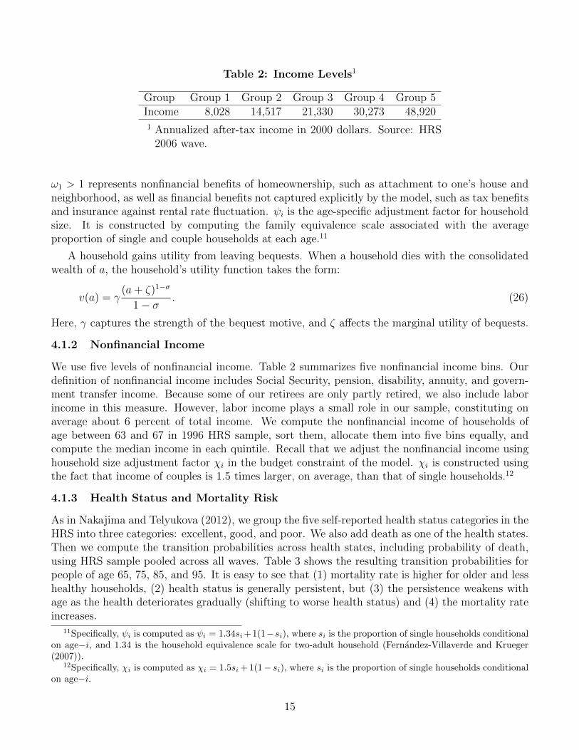
Table 2: Income Levels1

Group Group 1 Group 2 Group 3 Group 4 Group 5Income 8,028 14,517 21,330 30,273 48,9201 Annualized after-tax income in 2000 dollars. Source: HRS

2006 wave.

ω1 > 1 represents nonfinancial benefits of homeownership, such as attachment to one’s house andneighborhood, as well as financial benefits not captured explicitly by the model, such as tax benefitsand insurance against rental rate fluctuation. ψi is the age-specific adjustment factor for householdsize. It is constructed by computing the family equivalence scale associated with the averageproportion of single and couple households at each age.11

A household gains utility from leaving bequests. When a household dies with the consolidatedwealth of a, the household’s utility function takes the form:

v(a) = γ(a+ ζ)1−σ

1− σ. (26)

Here, γ captures the strength of the bequest motive, and ζ affects the marginal utility of bequests.

4.1.2 Nonfinancial Income

We use five levels of nonfinancial income. Table 2 summarizes five nonfinancial income bins. Ourdefinition of nonfinancial income includes Social Security, pension, disability, annuity, and govern-ment transfer income. Because some of our retirees are only partly retired, we also include laborincome in this measure. However, labor income plays a small role in our sample, constituting onaverage about 6 percent of total income. We compute the nonfinancial income of households ofage between 63 and 67 in 1996 HRS sample, sort them, allocate them into five bins equally, andcompute the median income in each quintile. Recall that we adjust the nonfinancial income usinghousehold size adjustment factor χi in the budget constraint of the model. χi is constructed usingthe fact that income of couples is 1.5 times larger, on average, than that of single households.12

4.1.3 Health Status and Mortality Risk

As in Nakajima and Telyukova (2012), we group the five self-reported health status categories in theHRS into three categories: excellent, good, and poor. We also add death as one of the health states.Then we compute the transition probabilities across health states, including probability of death,using HRS sample pooled across all waves. Table 3 shows the resulting transition probabilities forpeople of age 65, 75, 85, and 95. It is easy to see that (1) mortality rate is higher for older and lesshealthy households, (2) health status is generally persistent, but (3) the persistence weakens withage as the health deteriorates gradually (shifting to worse health status) and (4) the mortality rateincreases.

11Specifically, ψi is computed as ψi = 1.34si +1(1−si), where si is the proportion of single households conditionalon age−i, and 1.34 is the household equivalence scale for two-adult household (Fernandez-Villaverde and Krueger(2007)).

12Specifically, χi is computed as χi = 1.5si + 1(1− si), where si is the proportion of single households conditionalon age−i.

15

Table 3: Health Status Transition (Percent)

Health status transition (age 65) Health status transition (age 75)Dead Excellent Good Poor Dead Excellent Good Poor

Excellent 1.3 72.8 21.5 4.4 Excellent 3.9 60.1 26.9 9.2Good 2.2 25.8 53.3 18.7 Good 6.6 21.1 46.9 25.4Poor 9.6 6.1 20.7 63.7 Poor 16.3 3.8 17.6 62.3Health status transition (age 85) Health status transition (age 95)

Dead Excellent Good Poor Dead Excellent Good PoorExcellent 10.5 46.8 27.1 15.6 Excellent 28.5 29.5 19.8 22.3Good 14.7 17.0 37.8 30.5 Good 32.9 12.9 26.8 27.5Poor 28.8 5.1 13.2 52.9 Poor 56.9 4.2 13.6 25.3

Source: HRS.

0

10000

20000

30000

40000

65 75 85 95

Age

Expected medical expenditures (health = excellent)

Expected medical expenditures (health = good)

Expected medical expenditures (health = poor)

(a) Mid-Income, by Health

0

10000

20000

30000

40000

50000

65 75 85 95

Age

Expected medical expenditures (income group = 1)





(b) Good Health, by Income

Figure 4: Expected Mean OOP Medical Expenditure

4.1.4 Medical Expenditures

We estimate the distribution of log-out of pocket (OOP) medical expenditures by age, health, incomequintile and household size from a pooled 1996-2006 HRS sample of retirees. The mean, standarddeviation and probability of zero expenses are estimated as quartics in age, and include interactionterms between age and the other three variables. Under the assumption of log-normality of medicalexpenses, we then compute the expected mean and standard deviation of level medical expenses.Figure 4 reproduces expected mean medical expenses, for single households in the middle incomebin by health, and in good health by income bin. As we would expect, people in worse health payhigher expenses, as do those with higher income. Recall that in the household budget constraint,the medical expenses of each age group are adjusted by the same household size adjustment factoras for income, χi.

16

Table 4: Probability of Moving to Nursing Home (Percent)

Health statusAge Excellent Good Poor65 0.13 0.16 0.6075 0.41 1.19 1.8985 3.99 5.96 8.3195 22.76 18.28 15.83

Source: HRS.

4.1.5 Involuntary Nursing Home Moves

Using the pooled HRS sample from 1996-2006, we compute the 2-year probability that an individ-ual moves into a nursing home and simultaneously stops being a homeowner, conditional on thehousehold’s age and health status. Table 4 shows the probabilities for age 65, 75, 85, and 95. Weinterpret the event of moving into a nursing home with loss of homeownership as compulsory movesout of the house, which are important when considering a reverse mortgage loan that depends crit-ically on how long a household stays in the house. Not surprisingly, the probability is generallyhigher for older and less healthy individuals. There are two caveats to these estimates. First, notall elderly move into nursing homes involuntarily. If we take into account that some of the movesare voluntary, the probability that a household is forced to move out is upward-biased. On theother hand, some older retirees might move to their children’s homes instead of a nursing home.This consideration implies that the probability of a moving shock might be underestimated. Sincethe data limit how well we can identify these events, our estimates of the moving shock are the bestthey can be.

4.1.6 Housing and Interest Rate

We create 10 house size bins, by sorting house values of all homeowners of age 63-67 in 2006 HRSsample, equally allocating them into 10 bins, and computing the median value of each bin. Housingrequires maintenance, whose cost is a fraction δ of the house value. δ is set at 1.7 percent per year,which is the average depreciation rate of residential structures in National Income and ProductAccounts (NIPA). When a household sells the house, the sales cost, which is a fraction κ of thesales price, has to be paid. The selling cost of a house (κ) is set at 6.6 percent of the value ofthe house. This is the estimate obtained by Greenspan and Kennedy (2007). Grueber and Martin(2003) report the median selling cost of 7.0 percent of the value of the house.

The interest rate is set at 4 percent per year (8 percent biennially). For conventional mortgageloans, we assume a borrowing premium (ιm) of 1.6 percent annually. This is the average spreadbetween 30-year conventional mortgage loans and Treasury bills of the same maturity between 1977and 2009. Rent is the sum of maintenance costs (δ) and the conventional mortgage interest rate(r + ιm).

To calibrate idiosyncratic house price shocks, we assume that the house price is normalized toone in the initial period, and follows an AR(1) process thereafter. Contreras and Nichols (2010)estimate the AR(1) process of house prices for nine Census regions as well as the U.S. as a whole

17

Table 5: Selected Characteristics of the Initial Distribution, Age 65, 2006

Health status Tenure status Financial asset position1 (excellent) 0.46 Homeowner 0.88 Saver 0.792 (good) 0.32 Renter 0.12 Borrower 0.213 (poor) 0.22

Source: HRS.

Their estimate of the persistence parameter associated with the Census regions varies between0.704 and 0.940. Their estimate for the national sample is 0.811, which we use as our persistenceparameter. Their estimates for the standard deviation of the shocks from Census regions variesbetween 6.5 percent and 9.3 percent, while the estimate from the national sample is 7.9 percent.On the other hand, Flavin and Yamashita (2002) estimate the standard deviation of individualhouse prices using Panel Study of Income Dynamics (PSID) and obtain the standard deviation of14.2 percent. We use 14.2 percent as our standard deviation to house price shocks, since the shockin our model is associated with individual house value. The AR(1) process is discretized into afirst-order Markov process. Since one period in the model spans two years, while the house priceshocks constructed above are at annual frequency, we square the obtained Markov process to makeit into a biennial process.

4.1.7 Initial Type Distribution

The type distribution of age-65 households is constructed using the HRS 2006 wave. Table 5 exhibitsthe dimensions of the initial distribution that we have not already discussed. Half of the householdsare in excellent health. Homeownership rate is close to 90 percent. All retirees in our sample arenet savers; however, in the language of the model, the financial asset position includes secured debt.That is, the net financial position does not include the value of the house. By this measure, 79percent of our sample are in net positive financial position at age 65 and remaining 21 percent arein net negative financial position at age 65.

4.2 Second-Stage Estimation

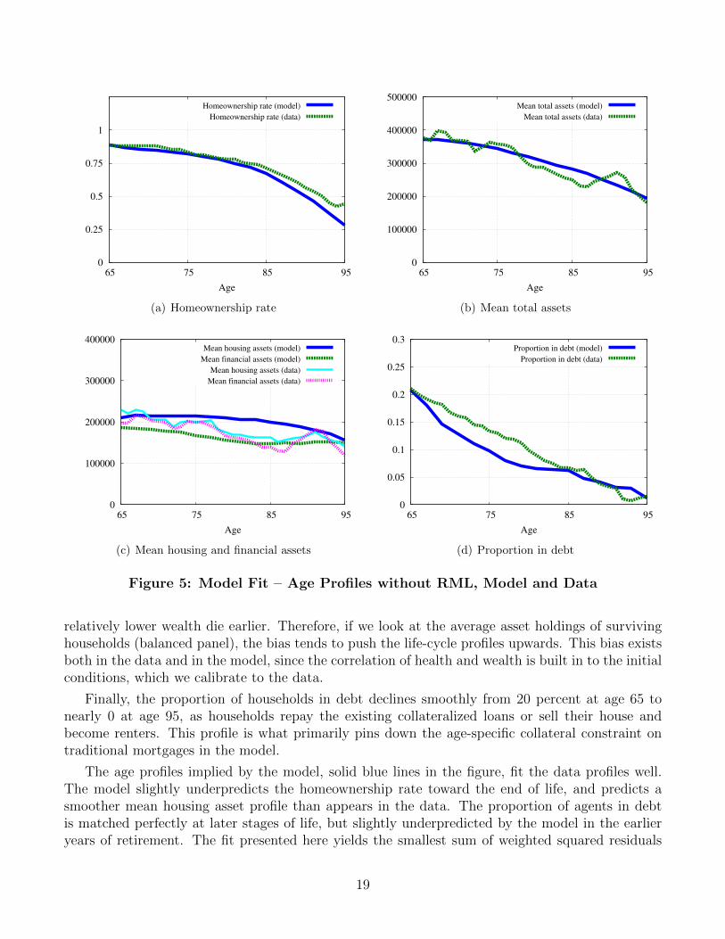
In the second-stage estimation, we match the cross-sectional age profiles of the homeownership rate,mean total, housing and financial asset holdings, and the proportion of retirees in debt. Again, wedo this in the baseline model that does not have reverse mortgages in it. Hence the debt here istraditional mortgage debt. Figure 5 shows the model fit. First, it is valuable to examine the dataprofiles – dashed green lines in the figure. The homeownership rate is 88 percent at age 65, anddeclines smoothly to about 40 percent by age 95. Mean total assets show a similarly smooth, butslow, decline, from about $375,000 to about $200,000. This high mean amount even at age 95 isthe statement of the classic “retirement saving puzzle” We analyze in detail the reasons for the lackof dissaving in this model in Nakajima and Telyukova (2012); there we show that housing plays acrucial role in the flatness of this profile.

Financial asset holdings do not decline much over the life-cycle for two of reasons. First, manyhouseholds sell their house towards the end of life, as seen in panel (a), which increases financialasset holdings at the expense of housing asset holdings. Second, there is a mortality bias; those with

18

0

0.25

0.5

0.75

1

65 75 85 95

Age

Homeownership rate (model)

Homeownership rate (data)

(a) Homeownership rate

0

100000

200000

300000

400000

500000

65 75 85 95

Age

Mean total assets (model)

Mean total assets (data)

(b) Mean total assets

0

100000

200000

300000

400000

65 75 85 95

Age

Mean housing assets (model)

Mean financial assets (model)

Mean housing assets (data)

Mean financial assets (data)

(c) Mean housing and financial assets

0

0.05

0.1

0.15

0.2

0.25

0.3

65 75 85 95

Age

Proportion in debt (model)

Proportion in debt (data)

(d) Proportion in debt

Figure 5: Model Fit – Age Profiles without RML, Model and Data

relatively lower wealth die earlier. Therefore, if we look at the average asset holdings of survivinghouseholds (balanced panel), the bias tends to push the life-cycle profiles upwards. This bias existsboth in the data and in the model, since the correlation of health and wealth is built in to the initialconditions, which we calibrate to the data.

Finally, the proportion of households in debt declines smoothly from 20 percent at age 65 tonearly 0 at age 95, as households repay the existing collateralized loans or sell their house andbecome renters. This profile is what primarily pins down the age-specific collateral constraint ontraditional mortgages in the model.

The age profiles implied by the model, solid blue lines in the figure, fit the data profiles well.The model slightly underpredicts the homeownership rate toward the end of life, and predicts asmoother mean housing asset profile than appears in the data. The proportion of agents in debtis matched perfectly at later stages of life, but slightly underpredicted by the model in the earlieryears of retirement. The fit presented here yields the smallest sum of weighted squared residuals

19

0

0.2

0.4

0.6

0.8

1

65 75 85 95

Age

Borrowing limit (conventional mortgage)

Borrowing limit (reverse mortgage)

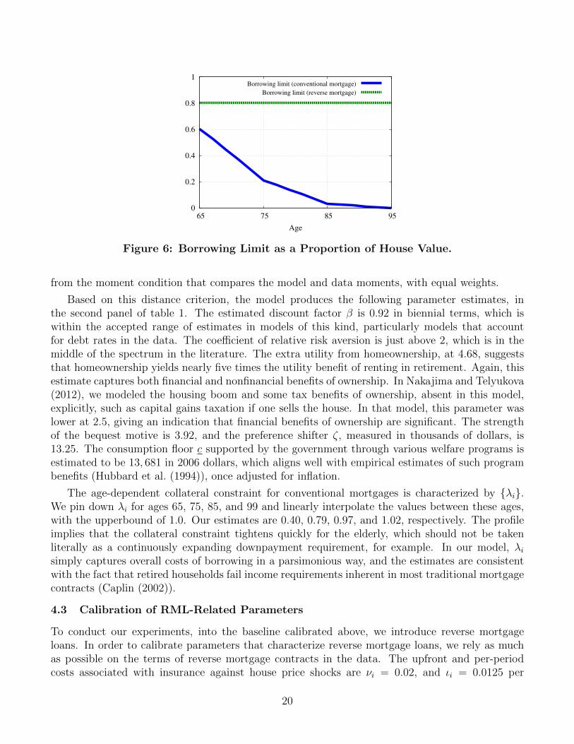
Figure 6: Borrowing Limit as a Proportion of House Value.

from the moment condition that compares the model and data moments, with equal weights.

Based on this distance criterion, the model produces the following parameter estimates, inthe second panel of table 1. The estimated discount factor β is 0.92 in biennial terms, which iswithin the accepted range of estimates in models of this kind, particularly models that accountfor debt rates in the data. The coefficient of relative risk aversion is just above 2, which is in themiddle of the spectrum in the literature. The extra utility from homeownership, at 4.68, suggeststhat homeownership yields nearly five times the utility benefit of renting in retirement. Again, thisestimate captures both financial and nonfinancial benefits of ownership. In Nakajima and Telyukova(2012), we modeled the housing boom and some tax benefits of ownership, absent in this model,explicitly, such as capital gains taxation if one sells the house. In that model, this parameter waslower at 2.5, giving an indication that financial benefits of ownership are significant. The strengthof the bequest motive is 3.92, and the preference shifter ζ, measured in thousands of dollars, is13.25. The consumption floor c supported by the government through various welfare programs isestimated to be 13, 681 in 2006 dollars, which aligns well with empirical estimates of such programbenefits (Hubbard et al. (1994)), once adjusted for inflation.

The age-dependent collateral constraint for conventional mortgages is characterized by {λi}.We pin down λi for ages 65, 75, 85, and 99 and linearly interpolate the values between these ages,with the upperbound of 1.0. Our estimates are 0.40, 0.79, 0.97, and 1.02, respectively. The profileimplies that the collateral constraint tightens quickly for the elderly, which should not be takenliterally as a continuously expanding downpayment requirement, for example. In our model, λisimply captures overall costs of borrowing in a parsimonious way, and the estimates are consistentwith the fact that retired households fail income requirements inherent in most traditional mortgagecontracts (Caplin (2002)).

4.3 Calibration of RML-Related Parameters

To conduct our experiments, into the baseline calibrated above, we introduce reverse mortgageloans. In order to calibrate parameters that characterize reverse mortgage loans, we rely as muchas possible on the terms of reverse mortgage contracts in the data. The upfront and per-periodcosts associated with insurance against house price shocks are νi = 0.02, and ιi = 0.0125 per

20

year, respectively. The reverse mortgage is further characterized by the triplet {λr, ιr, νr}, whichcaptures the collateral constraint, the interest premium, and the upfront cost. First, we set theinterest premium of the reverse mortgage loans to be the same as the conventional mortgages;ιr = 0.016 annually. Next, we set the borrowing limit at λr = 0.2, implying that any elderlyhousehold can borrow up to 80 percent of the value of their house through reverse mortgage loans.This is in line with the equity limits we see in the data. According to AARP, a 65-year-old RMLborrower can take a loan of up to 50 percent of their home value, while a 90-year old borrowercan access up to 75 percent. These numbers do not include interest and insurance costs, while inthe model, households pay these costs using the proceeds of the loan. Therefore, our borrowingconstraint, which is not age-dependent, is set slightly below the borrowing limit for a 90-year old,under the assumption that the expected interest cost for a 90-year old borrower is not too big.Figure 6 compares the borrowing limit of conventional and reverse mortgage loans in the model. Itis easy to see that reverse mortgage loans allow homeowners, especially the older ones, to borrowmore out of the value of their house, at various additional costs.

Finally, the upfront cost is calibrated such that the model replicates the empirical take-up ratein 2009, which is 1.36 percent of homeowners. The procedure yields νr = 0.096. This is the sum ofthe origination fee and the closing cost. The upfront cost of 9.6 percent of house value might be onthe higher side. In data, terms of reverse mortgage loans vary, but typical upfront cost appear tobe around 5 percent of house value. The origination fee is typically 2 percent of the house value upto 200, 000 dollars and 1 percent above it, with the cap of 6, 000 and the floor of 2, 500. Consideringthat most house values in the model are below 200, 000, but half of the houses are below 100, 000,where the floor of 2, 500 dollars binds, 2.5 percent is reasonable. The closing cost is typically around2, 000−3, 000. Dividing the amount by the median house value in the sample, we get 2.5 percent aswell. Therefore, we interpret the calibrated upfront cost νr = 0.096 as including both the monetarycosts of obtaining a reverse mortgage loans and other costs that are not explicitly modeled. Threeexamples come to mind. First, reverse mortgages in the model are more flexible than in the datain that borrowers can adjust the balance flexibly; in particular, they can prepay in order to avoidinterest and insurance premium flow costs for the balance that they have already taken out. Thiskind of prepayment appears restricted in the data. Second, the model ignores the high costs oflearning about reverse mortgages; for example, in order to qualify for an RML, potential borrowersare required to attend an informational seminar. The additional upfront costs in our calibrationcapture these information costs. Third, there might be a psychological or stigma cost attachedto obtaining an RML. Later, we show results based on νr = 0.05 instead of the baseline value ofνr = 0.096. The take-up rate of reverse mortgages associated with this lower upfront interest costcan be interpreted as the size of the pool of potential beneficiaries from reverse mortgage loans.

5 Results

5.1 Distribution of Reverse Mortgage Borrowers

Figure 7 shows two aspects of the age distribution of households who hold a reverse mortgage loanin the model. In particular, Panel (a) shows the distribution of the current age of reverse mortgageborrowers. Not surprisingly, it is hump-shaped; many of the households who have signed a reversemortgage earlier survive up to age 70s and 80s. Between age 85 and 95, the proportion declines ashouseholds with a reverse mortgage die or sell their house, voluntarily or involuntarily, and become

21

0

0.05

0.1

0.15

65 75 85 95

Age

Distribution of RML holders

(a) Age Distribution of RML Borrowers

0

0.05

0.1

0.15

0.2

0.25

65 75 85 95

Age

Distribution of age when RML is signed

(b) Age Distribution at RML Origination

Figure 7: Distribution of RML Borrowers

a renter. Panel (b) is the distribution of age at which a reverse mortgage loan is signed, amongall households who currently hold a reverse mortgage loan. This figure is a direct counterpart ofFigure 3. Four points stand out in the comparison. First, the levels are different, partly due todifferent age bins in the model and data. Each point in Panel (b) of Figure 7 captures two yearsof age, while each bar in Figure 3 captures only one year of age. Second, the general shape of thedistribution – initial spike and a hump shape after the initial spike – is quite similar between thetwo figures. Third, the initial spike in the data is at age 62, while it is at age 65 in the model. Thisis obviously because the initial age in the model corresponds to 65 years old, while reverse mortgageloans become available when a household (to be more precise, the youngest member of it) becomes62 years old. The initial age in the model is not set at 62 because a large proportion of householdsis still working and earning labor income, and thus is not fit for our sample of retirees. Fourth, ourmodel correctly predicts the drop-off of households who take a reverse mortgage later in their life.However, in the model, the peak of the distribution after the initial spike is between age 75 and 85,while the peak is around age 67 to 77 in the data. Some of this mismatch is mechanical and due tothe missing ages 62-64 in the model. This necessarily shifts the graph to the right.

5.2 Life-Cycle Profiles in Model with Reverse Mortgages

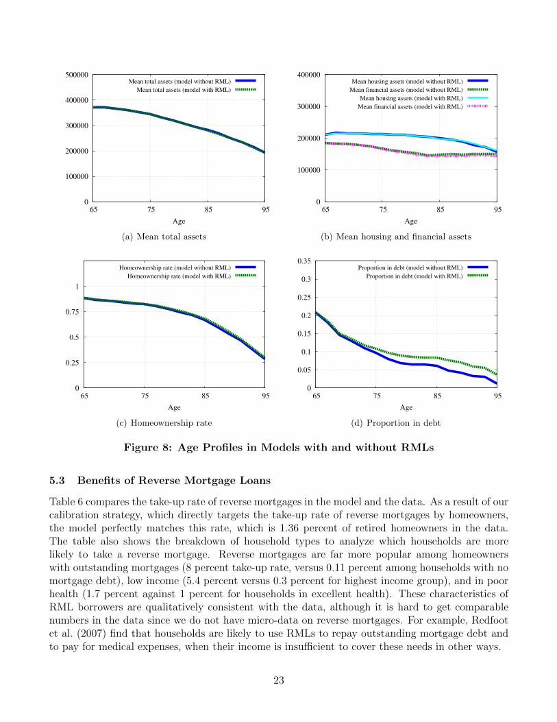
Figure 8 shows the life-cycle profiles discussed previously, in the model with reverse mortgagesrelative to the benchmark without. The aggregate effect for mean assets, be it total (panel (a)),financial or housing (panel (b)), is small, which is to be expected given the low take-up rate of reversemortgages (1.36 percent of retired homeowners). Notice that reverse mortgages enable people tostay in their house longer, which very slightly raises the homeownership rate in the model withRMLs (panel (c)). The most observable difference between the two models is in the proportion ofhouseholds who are in debt (panel (d)): this proportion is clearly higher in the model with reversemortgages, where retirees acquire a relatively flexible, if costly, means of borrowing against theirhome equity, compared with the more restrictive forward mortgage contracts that have incomerequirements usually failed by retirees.

22

0

100000

200000

300000

400000

500000

65 75 85 95

Age

Mean total assets (model without RML)

Mean total assets (model with RML)

(a) Mean total assets

0

100000

200000

300000

400000

65 75 85 95

Age

Mean housing assets (model without RML)

Mean financial assets (model without RML)

Mean housing assets (model with RML)

Mean financial assets (model with RML)

(b) Mean housing and financial assets

0

0.25

0.5

0.75

1

65 75 85 95

Age

Homeownership rate (model without RML)

Homeownership rate (model with RML)

(c) Homeownership rate

0

0.05

0.1

0.15

0.2

0.25

0.3

0.35

65 75 85 95

Age

Proportion in debt (model without RML)

Proportion in debt (model with RML)

(d) Proportion in debt

Figure 8: Age Profiles in Models with and without RMLs

5.3 Benefits of Reverse Mortgage Loans

Table 6 compares the take-up rate of reverse mortgages in the model and the data. As a result of ourcalibration strategy, which directly targets the take-up rate of reverse mortgages by homeowners,the model perfectly matches this rate, which is 1.36 percent of retired homeowners in the data.The table also shows the breakdown of household types to analyze which households are morelikely to take a reverse mortgage. Reverse mortgages are far more popular among homeownerswith outstanding mortgages (8 percent take-up rate, versus 0.11 percent among households with nomortgage debt), low income (5.4 percent versus 0.3 percent for highest income group), and in poorhealth (1.7 percent against 1 percent for households in excellent health). These characteristics ofRML borrowers are qualitatively consistent with the data, although it is hard to get comparablenumbers in the data since we do not have micro-data on reverse mortgages. For example, Redfootet al. (2007) find that households are likely to use RMLs to repay outstanding mortgage debt andto pay for medical expenses, when their income is insufficient to cover these needs in other ways.

23

Table 6: Take-up Rate of RMLs, Share of Homeowners

Take-up rate (percent)Data1

All homeowners 1.36ModelAll homeowners 1.36

No outstanding mortgages 0.11With outstanding mortgages 8.02

Low income 5.38Medium income 0.64High income 0.31

Poor health 1.72Good health 1.38Excellent health 1.041 2009 American Housing Survey.

Table 7: Welfare Gain from Reverse Mortgages, All Households

Welfare gain1 Proportion with gainAll households 510 0.863

No outstanding mortgages 437 0.844With outstanding mortgages 788 0.935

Low income 883 0.712Medium income 449 0.926High income 169 0.920

Poor health 588 0.837Good health 513 0.862Excellent health 467 0.8781 Welfare gain is measured by the one-time income at age 65 which

would make expected life-time utility of those with access to reversemortgages equal to expected life-time utility without. Measured in2006 dollars.

Table 7 quantifies the expected welfare gain from the availability of reverse mortgages. Thewelfare gain is measured as the one-time transfer at age 65, in 2006 U.S. dollars, that would makehouseholds in the economy without reverse mortgages indifferent, in expected terms, to being in the

24

Table 8: Impact of Uncertainty and Bequest Motives on RML Demand

Take-up rate, Welfare gain,homeowners all households1

Baseline model 1.36 510

No medical expense risks 0.91 314No medical expenses 0.85 308No moving shocks 1.65 749No house price shocks 1.61 303Expected house price boom 5.99 4161

No bequest motive 12.94 7188

No house price shocks, no medical expenses 1.40 200No moving shocks, no medical expenses 1.13 454No bequest motive, no medical expenses 20.02 85451 See note 1 of Table 7.

economy with RMLs. Note that no household in the model is worse off by having the option to buya reverse mortgage. Moreover, only homeowners gain from the introduction of reverse mortgages.However, these numbers are computed by averaging the welfare gain across all households, ownersand renters, in the economy. The welfare gain to households of living in a world with reversemortgages is equivalent to one-time transfer of $510 per person, and 86 percent of all the retirees(i.e. almost all the homeowners) value, ex-ante at age 65, the option of taking out a reverse mortgageat some point in the future, though most do not, ex-post. The welfare gain is higher among thosewho have outstanding traditional mortgages ($788 per person), because the RML gives them theability to keep borrowing against the value of their house, after they have to repay their conventionalmortgage debt (i.e., the borrowing limit associated with conventional mortgages tightens). Low-income households value the option more than high-income households, and those in poor healthmore than those in excellent health; in both cases, the ability to take a reverse mortgage at somepoint in the future is valuable for the purpose of relieving liquidity constraints, either due to lowincome or to large medical shocks. The percent of those who gain, ex-ante, from introduction ofRMLs in each line of the table reflects the proportion of homeowners in each group.

5.4 The Role of Bequest Motives and Uncertainty for Reverse Mortgage Take-Up

In this section, we investigate which elements of the retirees’ environment and behavior contributeto the low RML take-up rate. In particular, we focus on the role of different types of uncertaintythat retirees face, and then on the role of bequest motives. Since the main role of reverse mortgagesis to relax the borrowing constraint of homeowners in retirement, the demand for reverse mortgagescrucially depends on various elements that determine retirees saving and dissaving behavior. Table 8shows the take-up rate among homeowners in the model with several counterfactual experiments,as well as the associated welfare gains for all households, measured as before. First, we evaluate

25

the model without medical expenditure shocks; to do this, we assume that all households haveto pay the mean of the medical expenditure distribution, conditional on the current householdtype (age, income, and health status), in the baseline specification. In this case, the take-up ratedrops to 0.91 percent, all other things equal. If we shut off medical expenditures altogether, evenfewer households take a reverse mortgage (0.85 percent). These experiments demonstrate thatin the baseline specification, many households (about one-third of the total number) use reversemortgages to pay for medical expenses, especially larger ones, while staying in their homes. As aresult, without medical expense risk, the welfare gain from RMLs falls to $314 per household.

If the compulsory moving shocks are turned off, the take-up rate of reverse mortgages rises to1.7 percent of homeowners. This result echoes the result in Michelangeli (2010). The worst outcomefor RML borrowers is to face the compulsory moving shock shortly after paying the large upfrontcost of a reverse mortgage, but before utilizing the line of credit. This outcome is eliminated ifmoving shocks are turned off, which makes reverse mortgages more attractive as a way of relievingpossible liquidity constraints while staying in the house longer. In this case, the welfare gain risesto $749 per household.

Similarly, if house price shocks are turned off, the take-up rate increases to 1.6 percent ofhomeowner households. This increase might seem counterintuitive at first, because one of thebenefits of RMLs is their non-recourse nature. However, temporary house price shocks work in thesame way as moving shocks. If a household observes a temporary increase of the house value, itmay want to sell the house for the capital gain, even though holding on to the house gives extrautility. This implies that the expected duration of tenure as a homeowner is shorter with house priceshocks, and thus the value of reverse mortgages is lower. If the house price shocks are eliminated,homeowners can be certain to remain in their house longer, which makes reverse mortgage moreattractive. The welfare gain in the world without house price shocks is $303 per household, reflectinga reduction of risk.

Next, we add to the model the expectation of deterministic house price growth of 4.5 percentper year, which is the average real house price appreciation rate between 1996 and 2006. In thisexperiment, the take-up rate rises to 6 percent. This is intuitive: when households expect houseprice growth, they want to front-load consumption by borrowing more, which can be achieved bytaking reverse mortgages. In this case, the welfare gains for RML borrowers rise significantly, to$4161 per household. This experiment suggests that the observed fast increase in the take-up rate inthe period 2000-2009, shown in Figure 1, might be the result of expected house price appreciation.

Finally, we recompute the model without the bequest motive, setting γ = 0. In this scenario,the RML take-up rate increases tenfold, to about 13 percent of homeowners. It is intuitive thatbequest motives significantly dampen RML demand. Without bequest motives, many householdsdecumulate assets substantially more quickly, and reverse mortgages allow them to do so withoutmoving out of the house. Notice that in this case, the magnitude of the welfare gain to householdsfrom the availability of reverse mortgages is also very large compared to the benchmark case, at$7188 per household.

In the last set of experiments, we investigate in more detail how households in the model usereverse mortgages. As we established, in the model many homeowners use RMLs to pay for medicalexpenses. However, we also showed that some features of the environment dampen RML demandsignificantly. We want to evaluate to what extent, without these features, homeowners increase the

26

Table 9: Reverse Mortgage Loans with Alternative Terms

Take-up rate, Welfare gain,homeowners all households1

Baseline model 1.36 510

HECM Saver2 1.18 611Lower (0.5%) flow insurance premium 1.59 614No insurance (recourse) 1.93 873

Lower (5%) upfront cost 2.12 10001 See note 1 of Table 7.2 Upfront cost is lowered to 0.01 percent of the house value but the

borrower can access to up to 65 percent (instead of 80 percent) of thehome equity.

use of reverse mortgages for non-medical consumption. In the last three rows of table 8 , we answerthis question by shutting off medical expenses in the model without house price shocks, movingshocks, and bequest motives. In the world without moving shocks, 1.1 percent of homeownersuse RMLs for non-medical consumption; without house price shocks, 1.4 percent do. The dramaticresult comes in the world without bequest motives: here, 20 percent of households use RMLs for non-medical consumption. This explains the large welfare gains from RML loans that we documentedabove. Notice also that this take-up rate is higher than in the model without bequest motivesbut with medical expenses. This happens because medical expense shocks create a precautionarymotive, which dampens RML demand even if bequest motives are absent; households decumulateassets more slowly in anticipation of large medical expense shocks.

In sum, our model suggests that, conditional on the existing RML contract, low demand forreverse mortgages is in part an expression of the retirement saving puzzle: households do not takeout reverse mortgages for the same reasons that they do not decumulate their assets rapidly inretirement. Of course, this is subject to the costs of RMLs; we turn to the investigation of thesecosts next.

5.5 The Impact of Reverse Mortgage Terms on RML Demand

In this section, we explore how the demand for reverse mortgage loans is affected by their currentterms, in response to the popular claim that the high costs of RMLs are to blame. Table 9 summa-rizes the results. First, we consider the impact of a change in RML terms introduced in October2010 by the Federal Housing Administration. The FHA introduced a new type of RML known asthe HECM Saver. In order to reduce the oft-criticized upfront costs of reverse mortgage loans, theHECM Saver only requires upfront insurance premium of 0.01 percent of house value, down from 2percent. However, since a lower insurance premium exposes the government to larger house pricerisk, the amount of equity that a borrower can extract using HECM Saver has been lowered as well.The AARP states that this amount decreases by 10-18 percent, depending on the borrower age.

We consider RML demand in a counterfactual model economy where the HECM Saver, instead

27

of the regular reverse mortgage, is available. To do this, we make two changes to reverse mortgagesin the model: first, the upfront insurance premium is reduced to νi = 0.0001; second, reversemortgage borrowers can extract 15 percent less than in the baseline case, reflecting the AARPestimate and the fact that the tightest constraint must be on the youngest borrowers, who areexpected to live the longest. The first two rows of Table 9 compare the baseline model and thecounterfactual model with HECM Saver RMLs. We find that the take-up rate of reverse mortgageloans actually falls, from 1.4 percent to 1.2 percent of homeowners. The model thus predicts thathomeowners value access to additional equity more than lower insurance costs upfront. On the otherhand, interestingly, the average welfare gain of having the option to purchase the HECM Saver ishigher ($611) than the welfare gain in the model with the standard RML ($510). This implies thatthose who utilize the HECM Saver reverse mortgages benefit more than from the standard RMLthrough the lower upfront insurance premium.

It is important to keep in mind that this result does not mean that the HECM Saver is hurtingretired homeowners, because the Saver is available on top of the standard reverse mortgages inreality, while it replaces the regular reverse mortgage loans in the model. But the lower take-uprate in the model with the HECM Saver suggests that providing it in addition to the standardreverse mortgage loans would not create a substantial increase in the demand for reverse mortgageloans in general.

We also evaluate the impact of lowering the flow insurance cost. In the second counterfactualexperiment, we lower the mortgage insurance premium to 0.5 percent per year from 1.25 percentin the baseline. This comparison evaluates, in reverse, the increase in the premium introduced inOctober 2010, which resulted from falling house prices and the perceived increase in RML risk. Ascan be seen in the third row of Table 9, a lower insurance premium boosts the take-up rate slightly,to 1.6 percent, other things equal. Preliminary information suggests that the market for reversemortgage loans has been shrinking since 2010. Our model suggests that the increase in the premiummight be one of the triggers.

As we discussed, reverse mortgages offer a combination of benefits. First, borrowers can accessmore of their home equity. Second, with mandatory insurance, reverse mortgage loans offer insur-ance against house price declines, through their non-recourse nature. In the next experiment, wedisentangle the relative magnitude of the benefits by shutting off the insurance part of the reversemortgage loans. We do so by, first, setting insurance costs (ιi and νi) to zero, and second, makingthe RML a recourse loan. That is, we change the terms so when the borrower dies or moves outand the RML is consolidated, the borrower is liable for any excess loan amount. One point to notein this experiment is that households can always accumulate the RML balance and then default,using the consumption floor, when they sell the house; hence the loan cannot be made a perfectrecourse loan. However, this likely mirrors the possibility of default in the data as well.

The fourth row of Table 9 shows the take-up rate in the counterfactual model economy whereonly recourse reverse mortgage loans are available. Here, the take-up rate rises by 43 percent, to1.9 percent of homeowners. Notable also is the increase in the welfare gain from making RMLsrecourse loans: it rises to $873 per household. This suggests that, in our model, reverse mortgageborrowers do not value the insurance aspect of the RML. There are three reasons for this. First,most RML borrowers in the model carry relatively small balances of reverse mortgages when theloans become due, and thus the probability of being unable to repay is small. This feature ofthe model is consistent with the data. Second, borrowers have access to the publicly provided

28

consumption floor, which captures welfare programs such as Medicaid. This makes the additionalinsurance in the RML contract less valuable to elderly households. Third, since we do not model thebig swings in housing prices that has been observed since mid-2000s, we could be underestimatingthe house price risk that households face.

Finally, we discuss in Section 4.3 that the calibrated upfront interest cost (9.4 percent of thehouse value) is higher than the observed monetary upfront cost of obtaining a reverse mortgage(around 5 percent). Although we believe that the 9.4 number correctly captures some of the costs ofRMLs that are not explicitly in the model, we run an experiment where we assume that the upfrontinterest cost is 5 percent. We interpret the difference between the observed take-up rate and thetake-up rate in the model with the 5 percent cost as one of many possible measures of the marketpotential of reverse mortgage loans. As we discussed in Section 1 and footnote 1, Rasmussen etal. (1995) and Merrill et al. (1994) each compute the proportion of homeowners who would benefitfrom having the RML option, and get 80 percent and 9 percent, respectively. Although these andother studies estimate a broad range of numbers for this market potential, all seem to agree thatthe market for reserve mortgages can be substantially larger than the 1.36 percent take-up ratein 2009. It is often argued that one of the main reasons of such difference is that households donot know or do not know enough about reverse mortgages. The result of our last experiment (lastrow of Table 9) suggests that even when all households understand the benefits of RMLs, and theupfront costs are substantially lowered, the take-up rate less than doubles, to just 2.2 percent ofeligible homeowners.

6 Conclusion

In this paper, we analyze reverse mortgage loans using a calibrated structural model of life inretirement where elderly households make decision of consumption, savings, housing, and reversemortgages. When the modal is calibrated to match the observed take-up rate, the expected welfaregain of introducing reverse mortgages is sizable – equivalent to 500 dollars of one-time transferfor all households, and even higher for homeowners. Our model indicates that under the currentenvironment and RML terms, reverse mortgages are used by about one-third of the borrowers topay for medical expenses, while allowing them to remain their home. Not surprisingly, we alsofind that RMLs are particularly popular among lower-income and lower-wealth households, andhouseholds in poor health.

Through counterfactual experiments, we identify that, conditional on the RML contract as itexists in the data, bequest motives, involuntary nursing home moving shocks, and house pricefluctuations all dampen RML demand to various degrees. However, not surprisingly, we also findthat the costs of the RML contract are an important determinant of demand as well. In particular,the insurance costs inherent in the current RML contract dampen RML demand, because householdsdo not value this insurance, due to relatively low borrowed amounts and government-providedinsurance such as Medicaid. Along these lines, the model predicts a substantial increase in demandif the reverse mortgage were made a recourse loan. In addition, the HECM Saver loan of 2010, whichlowers the upfront insurance costs in exchange for lowering the total amount of equity accessible tothe borrower, actually lowers RML demand among homeowners, which suggests that adding thisoption to the already-existing RML contract is not likely to boost demand significantly. Finally,lowering only the upfront interest cost expands RML demand to only 2.2% of borrowers. Onepossible interpretation of these results is that given the risk that lenders have to take on to offer the

29

RML, the resulting contract is too expensive to be desirable to the vast majority of retirees. Thismay mean that given the costs of the reverse mortgage, many homeowners are better off sellingtheir homes in the event of needing to liquidate their home equity, as in Nakajima and Telyukova(2012).

We also find that if households expect a housing boom, that increases demand for reversemortgages because households would want to front-load consumption by borrowing, then repayfrom the capital gains. This may account for the rapid rise in demand for RMLs in 2000-2009.This suggests the question of what we may expect to happen to demand for reverse mortgagesgoing forward. The take-up rate of reverse mortgage loans could drop as the expected house pricegrowth rate tapers off after the Great Recession. At the same time, some homeowners might usereverse mortgages more extensively in response to the downturn, to relax the borrowing constraintthat they face. Our model cannot be used to formally evaluate these possibility, because we do notmodel changes in house price growth rates. We leave this issue for future research.

30

References

AARP, “Reverse Mortgage Loans: Borrowing Against Your Home,” 2010. AARP booklet.

Ameriks, John, Andrew Caplin, Steven Paufer, and Stijn van Nieuwerburgh, “The Joyof Giving or Assisted Living? Using Strategic Surveys to Separate Public Care Aversion fromBequest Motives.,” Journal of Finance, 2011, 66 (2), 519–561.

Campbell, John and Joao F. Cocco, “Household Risk Management and Optimal MortgageChoice,” Quarterly Journal of Economics, 2003, 118 (4), 1449–1494.

Caplin, Andrew, “Turning Assets into Cash: Problems and Prospects in the Reverse MortgageMarket,” in Olivia S. Mitchell, Zvi Bodie, Brett Hammond, and Steve Zeldes, eds., Innovationsin Retirement Financing, Philadelphia, PA: University of Pennsylvania Press, 2002, chapter 3,pp. 234–253.

Chambers, Matthew, Carlos Garriga, and Don E. Schlagenhauf, “The Loan Structure andHousing Tenure Decisions in an Equilibrium Model of Mortgage Choice,” Review of EconomicDynamics, 2009b, 12 (3), 444–468.

Contreras, Juan and Joseph Nichols, “Consumption Responses to Permanent and TransitoryShocks to House Appreciation,” 2010. FEDS Working Paper No. 2010-32.

Davidoff, Thomas, “Can ’High Costs’ Justify Weak Demand for the Home Equity ConversionMortgage?,” 2012. Unpulished.

De Nardi, Mariacristina, “Wealth Inequality and Intergenerational Links,” Review of EconomicStudies, 2004, 71 (3), 743–768.

, Eric French, and John Bailey Jones, “Why Do the Elderly Save? The Role of MedicalExpenses,” Journal of Political Economy, 2010, 118 (1), 39–75.

Dushi, Irena and Anthony Webb, “Household Annuitization Decisions: Simulations and Em-pirical Analysis,” Journal of Pension Economics and Finance, 2004, 3 (2), 109–143.

Fernandez-Villaverde, Jesus and Dirk Krueger, “Consumption over the Life Cycle: Factsfrom Consumer Expenditure Survey Data,” Review of Economics and Statistics, 2007, 89 (3),552–565.

Flavin, Marjorie and Takashi Yamashita, “Owner-Occupied Housing and the Composition ofthe Household Portfolio,” American Economic Review, 2002, 92 (1), 345–362.

Foote, Bruce E., “Reverse Mortgages: Background and Issues,” Congressional Research ServiceReport, 2010.

Greenspan, Alan and James Kennedy, “Sources and Use of Equity Extracted from Homes,”2007. Federal Reserve Board, FEDS Working Paper No. 2007-20.

31

Grueber, Joseph and Robert F. Martin, “The Role of Durable Goods in the Distribution ofWealth: Does Housing Make Us Less Equal?,” 2003. Board of Governors of the Federal ReserveSystem, International Finance Discussion paper No. 773.

Hubbard, R. Glenn, Jonathan Skinner, and Stephen P. Zeldes, “The Importance of Precau-tionary Motives in Explaining Individual and Aggregate Saving,” Carnegie-Rochester ConferenceSeries on Public Policy, 1994, pp. 59–125.

Hurd, Michael D., “Mortality Risk and Bequests,” Econometrica, 1989, 57 (4), 779–813.

Lockwood, Lee M., “Bequest Motives and the Annuity Puzzle,” Review of Economic Dynamics,forthcoming.

Merrill, Sally R., Meryl Finkel, and Nandinee Kutty, “Potential Beneficiaries from ReverseMortgage Products for Elderly Homeowners: An Analysis of American Housing Survey Data,”Real Estate Economics, 1994, 22 (2), 257–299.

Michelangeli, Valentina, “Does It Pay to Get a Reverse Mortgage?,” 2010. Unpublished.

Mitchell, Olivia S., James M. Poterba, and Mark J. Warshawsky, “New Evidence on theMoney’s Worth of Individual Annuities,” American Economic Review, 1999, 89 (5), 1299–1318.

Nakajima, Makoto, “Everything You Always Wanted to Know About Reverse Mortgages butWere Afraid to Ask,” Federal Reserve Bank of Philadelphia Business Review, First Quarter 2012,pp. 19–31.

and Irina A. Telyukova, “Home Equity in Retirement,” 2012. Mimeo, UCSD.

Pashchenko, Svetlana, “Accounting for Non-Annuitization,” 2004. Federal Reserve Bank ofChicago Working Paper No. 2010-03.

Rasmussen, David W., Issac F. Megbolugbe, and Barbara A. Morgan, “Using the 1990Public Use Microdata Sample to Estimate Potential Demand for Reverse Mortgage Products,”Journal of Human Resources, 1995, 6 (1), 1–24.

Redfoot, Donald L., Ken Scholen, and S. Kathi Brown, “Reverse Mortgages: Niche Prod-uct or Mainstream Solution? Report on the 2006 AARP National Survey of Rverse MortgageShoppers,” 2007. AARP Public Policy Institute.

Shan, Hui, “Reversing the Trend: The Recent Expansion of the Reverse Mortgage Market,” RealEstate Economics, 2011, 39 (4), 743–768.

Turra, Cassio M. and Olivia S. Mitchell, “The Impact of Health Status and Out-of-PocketMedical Expenditures on Annuity Valuation,” 2004. Pension Research Council Working paperNo. 2004-02, The Wharton School of the University of Pennsylvania.

Venti, Steven F. and David A. Wise, “Aging and Housing Equity: Another Look,” in David A.Wise, ed., Perspectives on the Economics of Aging, Chicago: University of Chicago Press, 2004,chapter 3, pp. 127–175.

32

Yaari, Menahem E., “Uncertain Lifetime, Life Insurance, and the Theory of the Consumer,”Review of Economic Studies, 1965, 32 (2), 137–150.

33

Reverse Mortgage Loans: A Quantitative Analysis - · PDF fileReverse Mortgage Loans: A Quantitative Analysis Makoto Nakajimay Federal Reserve Bank of Philadelphia Irina A. Telyukovaz

Documents