Reverend Bayes meets Darwin: Bayesian inference of phylogeny and its impact on evolutionary biology (Supplemental Material)

Reverend Bayes meets Darwin: Bayesian inference of phylogenyand its impact on evolutionary biology

(Supplemental Material)

John P. Huelsenbeck1, Fredrik Ronquist2, Rasmus Nielsen3 and Jonathan P. Bollback1

1Department of Biology, University of Rochester,Rochester, NY 14627, U.S.A.

2Department of Systematic Zoology, Evolutionary Biology Centre,Uppsala University, Norbyv. 18D, SE-752 36 Uppsala, Sweden

3Department of Biometrics, Cornell University,Ithaca, NY 14853-1643, U.S.A.

Bayesian inference1

A simple example of Bayesian inference

We will illustrate Bayesian inference using a simple example involving dice. Consider a box with 100dice, 90 of which are fair and 10 of which are biased. The probability of observing some number of pips afterrolling a fair or biased die is given in the following table:

Observation Fair Biased16

121

16

221

16

321

16

421

16

521

16

621

The probability of a high roll is larger for the biased dice than for the fair dice. Suppose that you draw adie at random from the box and roll it twice, observing a four on the first roll and a six on the second roll.What is the probability that the die is biased?

A Bayesian analysis combines ones prior beliefs about the probability of a hypothesis with the likelihood.The likelihood is the vehicle that carries the information about the hypothesis contained in the observations.In this case, the likelihood is simply the probability of observing a four and a six given that the die is biasedor fair. Assuming independence of the tosses, the probability of observing a four and a six is

Pr[ , | Fair] =16× 1

6=

136

for a fair die andPr[ , | Biased] =

421

× 621

=24441

1This section of the supplemental material is taken from the MrBayes manual.

1

for a biased die. The probability of observing the data is 1.96 times greater under the hypothesis that thedie is biased. In other words, the ratio of the likelihoods under the two hypotheses suggests that the die isbiased.

Bayesian inferences are based upon the posterior probability of a hypothesis. The posterior probabilitythat the die is biased can be obtained using Bayes’s (1) formula:

Pr[Biased | , ] =Pr[ , | Biased] × Pr[Biased]

Pr[ , | Biased] × Pr[Biased] + Pr[ , | Fair] × Pr[Fair]

where Pr[Biased] and Pr[Fair] are the prior probabilities that the die is biased or fair, respectively. As weset up the problem, a reasonable prior probability that the die is biased would be the proportion of the dicein the box that were biased. The posterior probability is then

Pr[Biased | , ] =24441 × 1

1024441 × 1

10 + 136 × 9

10

= 0.179

This means that our opinion that the die is biased changed from 0.1 to 0.179 after observing the four andsix.

Depending upon one’s viewpoint, the incorporation of prior beliefs about a parameter is either a strengthor a weakness of Bayesian inference. It is a strength in as much as the method explicitly incorporates priorinformation in inferences about a hypothesis. However, it can often be difficult to specify a prior. For thedice example, it is easy to specify the prior as we provided information on the number of fair and biased dicein the box and also specify that a die was randomly selected. However, if we were to simply state that thedie is either fair or biased, but did not specify a physical description of how the die was chosen, it would havebeen much more difficult to specify a prior specifying the probability that the die is biased. For example,one could have taken the two hypotheses to have been a priori equally probable or given much more weightto the hypothesis that had the die fair as severely biased dice are rarely encountered (or manufactured) inthe real world.

Bayesian inference of phylogeny

Bayesian inference of phylogeny is based upon the posterior probability of a phylogenetic tree, τ . Theposterior probability of the ith phylogenetic tree, τi, conditioned on the observed matrix of aligned DNAsequences (X) is obtained using Bayes’s formula:

f(τi|X) =f(X|τi)f(τi)∑B(s)

j=1 f(X|τj)f(τj)

[throughout, we denote conditional probabilities as f(·|·)]. Here, f(τi|X) is the posterior probability of the ithphylogeny and can be interpreted as the probability that τi is the correct tree given the DNA sequence data.The likelihood of the ith tree is f(X|τi) and the prior probability of the ith tree is f(τi). The summation inthe denominator is over all B(s) trees that are possible for s species. This number is B(s) = (2s−3)!

2s−2(s−2)! for

rooted trees, B(s) = (2s−5)!2s−3(s−3)! for unrooted trees, and B(s) = s!(s−1)!

2s−1 for labelled histories. Typically, anuninformative prior is used for trees, such that f(τi) = 1

B(s)

DNA sequence data.—We consider an aligned matrix of s DNA sequences:

X = {xij} =

Species 1Species 2Species 3

...Species s

A A C C T

A A C G G

A C C C T...

......

......

A C C C T

2

1 2 3 4 5

6

7

8

9

v1v5v4

v6v3

v2

v8v7

Figure 1.—An example of a phylogenetic tree for s = 5 species. The branch lengths are denoted vi.

The data matrix consists of the sequences for s species for c = 5 sites from a gene (c is the length of thealigned DNA sequences). The observations at the first site are x1 = {A, A, A, . . . , A}′. In general, theinformation at the ith site in the matrix is denoted xi.

Phylogenetic models.—What is the probability of observing the data at the ith site? To calculate thisprobability, we assume a phylogenetic model. A phylogenetic model consists of a tree (τi) with branchlengths specified on the tree (vi) and a stochastic model of DNA substitution. Figure 1 shows an exampleof a phylogenetic tree of s = 5 species. The tips of the tree are labeled 1, 2, . . . , s and the internal nodesof the tree are labeled s + 1, s + 2, . . . , 2s − 1; the root of the tree is always labeled 2s − 1. The lengths ofthe branches are denoted vi and are in terms of the number of substitutions expected to occur along the ithbranch. In general, the ancestor of node k will be denoted σ(k); the ancestor of node 4 is σ(4) = 8. Theancestor of the root is σ(2s − 1) = ∅.

The second part of the phylogenetic model consists of a stochastic model of DNA substitution. Here, thetypical assumption is that DNA substitution is a continuous-time Markov process. The heart of the modelis a matrix specifying the instantaneous rate of substitution from one nucleotide state to another:

Q = {qij} =

· πCrAC πGrAG πT rAT

πArAC · πGrCG πT rCT

πArAG πCrCG · πT rGT

πArAT πCrCT πGrCT ·

where the matrix specifies the rate of change from nucleotide i (row) to nucleotide j (column). The nucleotidesare in the order A, C, G, T. The diagonals of the matrix are specified such that the rows each sum to 0. Theequilibrium (or stationary) frequencies of the four nucleotides are denoted πi (π = {πA, πC , πG, πT }). Thismatrix specifies the most general time-reversible model of DNA substitution and is referred to as the GTRmodel (2). Because the rate of substitution and time are confounded, the Q matrix is rescaled such that−

∑πiqii = 1 for all i (making the average rate of substitution 1). Over a branch of length v the transition

probabilities are calculated as P(v,θ) = {pij(v,θ)} = eQv. The parameters of the substitution model arecontained in a vector θ.

The likelihood of a phylogeny.—The phylogenetic model consists of a tree (τi) with branch lengths (vi) anda stochastic model of DNA substitution that is specified by a matrix of instantaneous rates. The probabilityof observing the data at the ith site in the aligned matrix is a sum over all possible assignments of nucleotidesto the internal nodes of the tree:

f(xi|τj ,vj ,θ) =∑

y

[πy2s−1

(s∏

k=1

pyiσ(k),xik(vk,θ)

) (2s−2∏

k=s+1

pyiσ(k),yik(vk,θ)

)]

Here, yij is the (unobserved) nucleotide at the jth node for the ith site. The summation is over all 4s−1

3

A

A

AC C

T

T

AC C

G

T

AC C

C

T

AC C

A

T

AC C

T

G

AC C

G

G

AC C

C

G

AC C

A

G

AC C

T

C

AC C

G

C

AC C

C

C

AC C

A

C

AC C

T

A

AC C

G

A

AC C

C

A

AC C

Figure 2.—The 16 possible assignments of nucleotides to the internal nodes of a tree of s = 3 species. Theobservations at the site are xi = {C, C, A} and the unobserved nucleotides at the internal nodes of the treeare denoted y.

ways that nucleotides can be assigned to the internal nodes of the tree. Figure 2 illustrates the possiblenucleotide assignments for a simple tree of s = 3 species. Felsenstein (3) introduced a pruning algorithmthat efficiently calculates the summation. Often, the rate at the site is assumed to be drawn from a gammadistribution. This allows one to relax the assumption that the rate of substitution is equal across all sites.If gamma-distributed rate variation is assumed, then the probability of observing the data at the ith sitebecomes:

f(xi|τj ,vj ,θ, α) =∫ ∞

0

{∑y

[πy2s−1

(s∏

k=1

pyiσ(k),xik(vkr, θ)

) (2s−2∏

k=s+1

pyiσ(k),yik(vkr, θ)

)]}f(r|α) dr

where f(r|α) is the density of the rate r under the gamma model (4). The parameter α is the shape parameterof the gamma distribution (here, the shape and the scale parameters of the gamma distribution are both setto α). Typically, this integral is impossible to evaluate. Hence, an approximation first suggested by Yang(5) is used in which the continuous gamma distribution is broken into K categories, each with equal weight.The mean rate from each category represents the rate for the entire category. The probability of observingthe data at the ith site then becomes:

f(xi|τj ,vj ,θ, α) =K∑

n=1

{∑y

[πy2s−1

(s∏

k=1

pyiσ(k),xik(vkrn,θ)

) (2s−2∏

k=s+1

pyiσ(k),yik(vkrn,θ)

)]}1K

Assuming independence of the substitutions across sites, the probability of observing the aligned matrix ofDNA sequences is

f(X|τj ,vj ,θ, α) =c∏

i=1

f(xi|τj ,vj ,θ, α)

Importantly, the likelihood can be calculated under a number of different models of character change. Forexample, the codon model describes the substitution process over triplets of sites (a codon) and allows theestimation of the nonsynonymous/synonymous rate ratio (6, 7). Similarly, models of DNA substitution havebeen described that allow nonindenpendent substitutions to occur in stem regions of rRNA genes (8). Finally,

4

one can calculate likelihoods for amino acid (9), restriction site (10), and, more recently, morphological data(11).

Bayesian inference of phylogeny.—As described so far, the likelihood depends upon several unknownparameters; generally, the phylogeny, branch lengths, and substitution parameters are unknown. The methodof maximum likelihood estimates these parameters by finding the values of the parameters which maximizethe likelihood function. Currently, programs such as PAUP* (12), PAML (13), and PHYLIP (14) estimatephylogeny using the method of maximum likelihood.

Bayesian inference is based instead upon the posterior probability of the parameter. As described above,the posterior probability of the ith tree is

f(τi|X) =f(X|τi)f(τi)∑B(s)

j=1 f(X|τj)f(τj)

where the likelihood function is integrated over all possible values for the branch lengths and substitutionparameters:

f(X|τi) =∫

vi

∫θ

∫α

f(X|τi,vi,θ, α)f(vi)f(θ)f(α) dvi dθ dα

Markov chain Monte Carlo.—Typically, the posterior probability cannot be calculated analytically. How-ever, the posterior probability of phylogenies can be approximated by sampling trees from the posterior prob-ability distribution. Markov chain Monte Carlo (MCMC) can be used to sample phylogenies according totheir posterior probabilities. The Metropolis-Hastings (MH) algorithm (15, 16, 17) is an MCMC algorithmthat has been used successfully to approximate the posterior probabilities of trees (18, 19).

The MH algorithm works as follows. Let Ψ = {τ, v,θ, α} be a specific tree, combination of branch lengths,substitution parameters, and gamma shape parameter. The MH algorithm constructs a Markov chain thathas as its stationary frequency the posterior probability of interest (in this case, the joint posterior probabilityof τ , v, θ, and α). The current state of the chain is denoted Ψ. If this is the first generation of the chain, thenthe chain is initialized (perhaps by randomly picking a state from the prior). A new state is then proposed,Ψ′. The probability of proposing the new state given the old state is f(Ψ′|Ψ) and the probability of makingthe reverse move (which is never actually made) is f(Ψ|Ψ′). The new state is accepted with probability

R = min(

1,f(Ψ′|X)f(Ψ|X)

× f(Ψ|Ψ′)f(Ψ′|Ψ)

)

= min(

1,f(X|Ψ′)f(Ψ′)/f(X)f(X|Ψ)f(Ψ)/f(X)

× f(Ψ|Ψ′)f(Ψ′|Ψ)

)

= min

1,

f(X|Ψ′)f(X|Ψ)︸ ︷︷ ︸

Likelihood Ratio

× f(Ψ′)f(Ψ)︸ ︷︷ ︸

Prior Ratio

× f(Ψ|Ψ′)f(Ψ′|Ψ)︸ ︷︷ ︸

Proposal Ratio

A uniform random variable between 0 and 1 is drawn. If this number is less than R, then the proposed stateis accepted and Ψ = Ψ′. Otherwise, the chain remains in the original state. This process of proposing a newstate, calculating the acceptance probability, and either accepting or rejecting the proposed move is repeatedmany thousands of times. The sequence of states visited forms a Markov chain. This chain is sampled (eitherevery step, or the chain is “thinned” and samples are taken every so often). The samples from the Markovchain form a valid, albeit dependent, sample from the posterior probability distribution (20). As describedhere, the Markov chain samples from the joint probability density of trees, branch lengths, and substitutionparameters. The marginal probability of trees can be calculated by simply printing to a file the trees that

5

-250000

-200000

-150000

-100000

-50000

0

0 500000 100000015000002000000

Generation

-40000

-39950

-39900

-39850

-39800

-39750

-39700

0 500000 100000015000002000000

Generation

Flavivirus

-12000

-11000

-10000

-9000

-8000

-7000

-6000

0 500000 100000015000002000000-6400

-6300

-6200

-6100

-6000

0 500000 100000015000002000000

Astragalus

Generation Generation

log e

L

log e

Llo

g eL

log e

L

Flavivirus

Astragalus

-140000

-120000

-100000

-80000

-60000

0 1000000200000030000004000000-70900

-70800

-70700

-70600

-70500

-70400

0 1000000200000030000004000000

Angiosperm atpB

-22500

-20000

-17500

-15000

-12500

-10000

0 500000 100000015000002000000

Generation

-12600

-12500

-12400

-12300

0 500000 100000015000002000000

Generation

Butterfly

Generation Generation

log e

Llo

g eL

log e

Llo

g eL

Angiosperm atpB

Butterfly

Figure 3.—Plots of the log probability of observing the data (loge L) through time for each of the four datasets.

are visited during the course of the MCMC analysis. The proportion of the time any single tree is found inthis sample is an approximation of the posterior probability of the tree.

Programs for Bayesian inference of phylogeny.—There are a few programs for the Bayesian analysis ofphylogenetic trees. BAMBE (22) and MrBayes (23) approximate the posterior probability of phylogeniesusing MCMC (specifically, the MH algorithm). BAMBE assumes uniform priors on phylogenies and branchlengths. The program uses an improved method for calculating likelihoods that is very fast. MrBayes imple-ments a larger number of substitution models and priors for parameters. Another program, MCMCTREE inthe PAML package of programs (13) calculates posterior probabilities of trees using a combination of MonteCarlo and MCMC integration. The program works for up to s = 11 species. Besides the algorithm forapproximating posterior probabilities, the program differs from BAMBE in assuming a birth-death processprior on phylogenies. This prior places equal weight on labelled histories (where a labelled history differsfrom a rooted tree in considering the relative speciation times).

Inferring large trees

Evidence for convergence in topology

In all of our analyses we ran at least two Markov chains, each of which started from a random tree. Eachchain consists of a total of n = 4 chains, all except one of which are heated. Each of these chains was alsostarted from a randomly chosen tree. We examined a number of diagnostics to determine if the chains hadreached stationarity. For one, we examined the correlation between the posterior probabilities of individualclades found in both chains. These results are depicted in the full paper and show that the inferences thatwould be drawn from different chains are largely the same. Another way of examinining convergence is tolook at the behavior of one or more parameters through time. For example, we examined the log probabilityof observing the data through time for the chains. These results are shown in Figure 3. The chains start withtrees that poorly explain the data but rapidly find better trees, eventually sampling trees which fluctuatearound a specific log probability.

We also examined the topological variance between and within chains to check for convergence. Beforeconvergence on the target distribution is reached, the trees from separate chains will tend to be more differentthan trees from a single chain. When the chains have reached the target distribution, the mean topologicaldistance will be the same within and among chains. Thus, convergence can be monitored by comparing the

6

mean topological distance within chains (W) and between chains (B). Initially, the ratio B/W is likely tobe considerably larger than 1. When the ratio is close to 1.0, it is likely that the chains have converged tothe target distribution. Robinson and Foulds measure of topological distance was used (24); it is equivalentto twice the number of unique taxon bipartitions found in one of the two trees but not in both. The meantopological distance within each chain was estimated by drawing 1000 or 5000 random pairs of trees fromthe chain. The mean topological distance within chains is simply the mean of the means for each chain.The mean topological distance between chains was estimated by drawing 1000 or 5000 random pairs of treesfrom different chains. All chains were started from random trees. This means that the topological distancebetween chains was initially close to the maximum value, equivalent to twice the number of taxa in theanalysis minus 6. Thus, the initial topological distance between chains was close to 206 for the butterflyanalysis, 240 for the flavivirus analysis, 274 for the Astragalus analysis, and 708 for the angiosperm analysis.

Flavivirus Mean topological distanceTrees sampled Draws Chain 1 Chain 2 Within (W) Between (B) Ratio B/W

625-1250 1000 71.24 43.10 57.17 98.33 1.7201250-2500 1000 48.15 31.62 39.89 44.65 1.1192500-5000 1000 34.34 33.95 34.14 35.00 1.0255000-10000 1000 36.41 42.01 39.21 40.74 1.03910000-20000 1000 37.61 44.15 40.88 41.89 1.0255000-20000 1000 38.15 44.45 41.30 41.79 1.011

Butterfly Mean topological distanceTrees sampled Draws Chain 1 Chain 2 Within (W) Between (B) Ratio B/W

625-1250 1000 87.10 68.20 77.65 100.99 1.3001250-2500 1000 85.36 63.96 74.66 85.05 1.1392500-5000 1000 74.27 68.71 71.49 75.19 1.0525000-10000 1000 71.05 64.44 67.75 68.63 1.01310000-20000 1000 74.19 69.38 71.78 72.95 1.0165000-20000 1000 73.90 67.84 70.87 71.67 1.011

Astragalus Mean topological distanceTrees sampled Draws Chain 1 Chain 2 Within (W) Between (B) Ratio B/W

625-1250 1000 124.51 152.62 138.56 150.55 1.0871250-2500 1000 121.26 113.45 117.35 122.38 1.0432500-5000 1000 115.64 114.69 115.16 117.46 1.0205000-10000 1000 116.02 118.80 117.41 118.53 1.00910000-20000 1000 117.42 117.55 117.49 117.62 1.0015000-20000 5000 117.41 118.69 118.05 118.27 1.002

Angiosperm atpB Mean topological distanceTrees sampled Draws Chain 1 Chain 2 Within (W) Between (B) Ratio B/W

1250-2500 1000 178.16 273.99 226.08 348.42 1.5412500-5000 1000 119.18 212.42 165.80 223.42 1.3485000-10000 1000 123.27 161.71 142.49 156.23 1.09610000-20000 1000 126.21 134.63 130.42 135.22 1.03720000-40000 1000 123.20 123.67 123.43 126.13 1.02210000-40000 1000 125.98 128.75 127.36 129.52 1.017

7

0

100

200

300

400

500

100 1000 10000 100000 1000000

dT

c = 100

s = 128

s = 256

0

100

200

300

400

500

100 1000 10000 100000 1000000

Generation

c = 1000

s = 128

s = 256

dT

Generation

Figure 4.—MCMC converges to the correct tree in simulation. DNA sequences were simulated under theJukes-Cantor model on symmetrically branching trees of s = 128 or s = 256 species. All of the branches ofthe trees were 0.1 expected substitution per site in length. The graphs show the topological distance, dT (1),from the true tree through time for chains that started from randomly chosen trees. The topological distanceeither plateaus near the true tree for the short sequences (c = 100) or to the true tree for the long sequences(c = 1000). Bayesian analysis assumed the correct model of DNA substitution.

Finally, we examined the ability of the MCMC method to converge to the correct tree(s) by performingsimulations of 128 and 256 sequences. Sequences were simulated under the Jukes-Cantor model of DNAsubstitution. In all simulation replicates, the chains converged to trees that were either identical to or veryclose to the true tree (Figure 4).

8

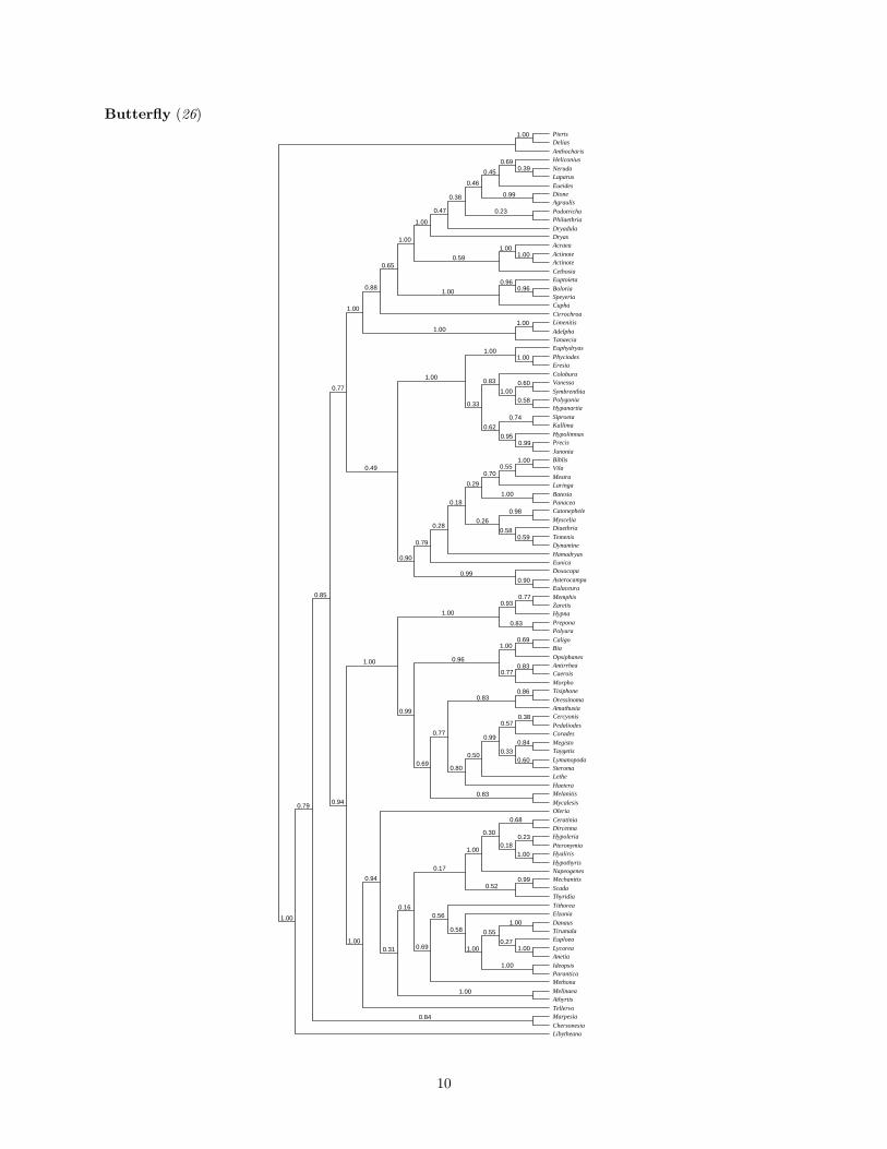
Phylogenetic trees

For each data set, we constructed a 50% majority rule consensus tree of the trees sampled by the MCMCprocedure. The numbers at the interior nodes indicate the posterior probability that the clade is correct underthe model. Polytomious nodes indicate that various resolutions of the polytomy have posterior probabilitiesless than 0.5.Flavivirus (25)

MVEJEZ34094JE826309JEZ34095JEZ34097JEM73710NakayamaSaigonBeijingP3HK8526IndonesiaDH20JED90195JEU04522SA14 USAKamiyamaThailandJEZ34096S892JEM18370KUNWNSLEDen1M87512Den1D00505Den1c92Den1D00502Den1D00503Den1D00501Den1X76219Den1BR90DEN3D3Philip56D3Indon73D3Tahiti89D3Indon75D3Indon78D3Indon85D3Malay74D3Philip83D3Thail86D3Thail87D3Thail73D3Thail62D3India84D3Moza85D3SLanka91D3SLanka89D3Lanka81D3SLanka85D3Samoa86D3PRico77D3Tahiti65D3PRico63Den2M29095Den2m24450Den2d00346Den2m24451Den2M84727Den2m24446Den2m24445Den2x15434Den2d00345Den2d10514Den2110050Den2m24449DEN2SL975DEN2SL206DEN2SEY42DEN2SEY52Den2110054Den5110055Den2110051DEN2BURKFADEN2INDONDen2m24448Den2m15075DEN2BrazilDen2m24444Den2x15214Den2110052DEN2PHILIPDEN2INDIADen254319Den2m19197DEN2PR159DEN4DE4Domin80DE4Phile56YFYFVCGYFVCAPSIDMYFVENVAYFVENVBYFVCMENSSRETYUPOWKFDLGTOHFFETBEFETBE 205TBEVsWTBEGGETSESSEIrishMa54LI ILI 31LI MLI SB526LI 261LI GLI 369LI ALI KNegishiLI 917LI NORCFA

0.56

0.780.80

0.81

0.83

0.86

0.87

0.88

0.92

0.92

0.92

0.98

1.00

1.00

1.00

0.92

1.00

0.46

0.93

0.67

0.980.83

0.96

0.99

0.581.00

1.001.00

1.00

1.001.00

0.98

0.230.22

0.99

0.731.00

1.00

1.00

1.00

1.00

1.00

1.00

1.00

0.79

1.00

1.00

1.00

1.00

1.00

1.00

1.00

0.84

1.00

1.00

1.00

1.00

0.470.97

1.000.96

1.001.00

1.00

0.91

0.92

0.921.00

0.84

1.00

0.64

0.97

1.00

0.60

0.58

0.691.00

0.36

0.37

1.00

0.89

1.00

1.001.00

1.00

1.00

1.00

1.001.00

0.93

1.00

1.00

1.001.00

1.00

1.00

1.00

0.581.00

0.41

1.001.00

1.000.76

0.760.94

0.95

1.00

0.950.97

0.97

0.79

0.83

0.45

0.49

0.81

0.85

0.760.42

0.39

9

Butterfly (26)PierisDelias

AnthocharisHeliconius

NerudaLaparus

EueidesDioneAgraulis

PodotrichaPhilaethria

DryadulaDryasAcraea

ActinoteActinote

CethosiaEuptoieta

BoloriaSpeyeriaCupha

CirrochroaLimenitis

AdelphaTanaeciaEuphydryas

PhyciodesEresia

ColoburaVanessa

SymbrenthiaPolygoniaHypanartia

SiproetaKallima

HypolimnasPrecis

JunoniaBiblisVila

MestraLaringa

BatesiaPanaceaCatonephele

MysceliaDiaethria

TemenisDynamine

HamadryasEunicaDoxocopa

AsterocampaEulaceura

MemphisZaretisHypna

PreponaPolyura

CaligoBia

OpsiphanesAntirrheaCaerois

MorphoTisiphone

OressinomaAmathusiaCercyonis

PedaliodesCorades

MegistoTaygetis

LymanopodaSteromaLethe

HaeteraMelanitis

MycalesisOleria

CeratiniaDircennaHypoleria

PteronymiaHyaliris

HypothyrisNapeogenesMechanitis

ScadaThyridia

TithoreaElzunia

DanausTirumalaEuploea

LycoreaAnetia

IdeopsisParanticaMethona

MelinaeaAthyrtis

TellervoMarpesia

ChersonesiaLibytheana

1.00

1.00

0.79

0.85

0.77

1.00

0.88

0.65

1.00

1.00

0.47

0.38

0.46

0.45

0.690.39

0.99

0.23

0.59

1.001.00

1.00

0.960.96

1.001.00

0.49

1.00

1.001.00

0.33

0.83

1.000.60

0.58

0.62

0.74

0.950.99

0.90

0.79

0.28

0.18

0.29

0.700.55

1.00

1.00

0.26

0.98

0.580.59

0.990.90

0.94

1.00

1.00

0.930.77

0.83

0.99

0.96

1.000.69

0.770.83

0.69

0.77

0.830.86

0.80

0.50

0.99

0.570.38

0.330.84

0.60

0.83

1.00

0.94

0.31

0.16

0.17

1.00

0.30

0.68

0.180.23

1.00

0.520.99

0.69

0.56

0.58

1.00

0.55

1.00

0.271.00

1.00

1.00

0.84

10

Astragalus (27)Astragalus paposanusAstragalus pehuenchesAstragalus asymmetricusAstragalus oxyphysusAstragalus nuttalliiAstragalus douglassiiAstragalus allochrousAstragalus thurberiAstragalus pachypusAstragalus mollissimusAstragalus calycosusAstragalus neuquenensisAstragalus arnottianusAstragalus patagonicusAstragalus palenae var grandifAstragalus palenae var palenaeAstragalus moyanoiAstragalus unidentAstragalus pickeringiiAstragalus garbancilloAstragalus arizonicusAstragalus nothoxysAstragalus arthuriAstragalus monoensisAstragalus inyoensisAstragalus speirocarpusAstragalus tetrapterusAstragalus collinusAstragalus alvordensisAstragalus filipesAstragalus curvicarpusAstragalus eremiticusAstragalus cibariusAstragalus chamaemeniscusAstragalus utahensisAstragalus purshiiAstragalus lentiginosusAstragalus salmonisAstragalus caricinusAstragalus sheldoniAstragalus reventusAstragalus obscurusAstragalus spatulatusAstragalus sesquiflorusAstragalus ceramicusAstragalus cremnophylaxAstragalus oocalycisAstragalus preussiAstragalus praelongusAstragalus asclepiadoidesAstragalus woodruffiiAstragalus linifoliusAstragalus kentrophytaAstragalus didymocarpusAstragalus cobrensisAstragalus tenellusAstragalus miserAstragalus molybdenusAstragalus shultziorumAstragalus rusbyiAstragalus brandegeiAstragalus monumentalisAstragalus scopulorumAstragalus bisulcatusAstragalus polarisAstragalus neglectusAstragalus lindheimeriAstragalus rattaniiAstragalus tenerAstragalus sabulonumAstragalus leptaleusAstragalus gilviflorusAstragalus aretioidesAstragalus humillimusAstragalus halliiAstragalus nuttallianusAstragalus lonchocarpusAstragalus bodiniAstragalus echinatusAstragalus cicerAstragalus chaborasicusAstragalus adsurgensAstragalus asteriasAstragalus tribuloidesAstragalus pulchellusAstragalus agrestisAstragalus cerasocrenusAstragalus echidnaeformisAstragalus peristereusAstragalus alpinusAstragalus polycladusAstragalus nankotaizanensisAstragalus australisAstragalus williamsiiAstragalus robbinsiiAstragalus eucosmusAstragalus siliquosusAstragalus corrugatusAstragalus oreganusAstragalus canadensisAstragalus falcatusAstragalus boeticusAstragalus edulisAstragalus cymbicarposAstragalus hamosusAstragalus americanusAstragalus umbellatusAstragalus membranaceusAstragalus chinensisAstragalus alopeciasAstragalus atropilosulusAstragalus cysticalyxSphaerophysa salsulaEremosparton flaccidumSmirnoviaSutherlandia frutescensLessertia herbaceaLessertia brachystachyaColutea arborescensAstragalus sinicusAstragalus complanatusClianthus puniceusCarmichaelia williamsiiCarmichaelia stevensoniiSwainsona pterostylisAstragalus vogeliiAstragalus epiglottisBiserrula pelecinusOxytropis splendensOxytropis viscidaOxytropis sericeaOxytropis campestrisOxytropis oreophilaOxytropis lambertiiOxytropis multicepsOxytropis besseyiOxytropis pilosaOxytropis szovitsiiOxytropis deflexaCaragana arborescens

1.00

0.94

0.58

1.00

0.96

1.00

1.00

0.96

0.67

1.00

0.94 1.000.96

0.81

0.99

0.74

0.95

1.00

0.97

0.94

0.99

0.99

0.860.93

0.750.59

0.910.83

0.630.50

0.98

1.00

0.950.99

0.96

0.89

0.59

0.98

0.520.97

0.89

0.80

0.96

1.000.96

0.721.00

1.00

1.000.99

1.00

1.00

1.00

1.001.00

0.780.99

0.62

1.001.00

1.001.00

1.00

0.61

0.75

0.91

0.82

1.00

0.56

0.991.00

1.00

1.000.93

1.00

0.991.00

1.00

0.88

1.00

1.00

0.67

0.93

0.99

1.00

0.97

11

Angiosperms (Part 1) (28)NicotianaSolanumIpomoeaBoragoHydrophyllumAntirrhinumSaintpauliaBuddlejaCatalpaGlobulariaLavandulaProsthanteraThunbergiaUtriculariaVerbenaJasminumBouvardiaRubiaCinchonaCoffeaDishidiaPlumeriaStrychnosOncothecaAucubaGarryaEucommiaPyrencanthaApiumHederaPittosporumBerzeliaSambucusViburnumValerianaCampanulaLobeliaRousseaCichoriumMenyanthesCorokiaPhellineEscalloniaGonocaryumHelwingiaIlexNemopanthusActinidiaCyrillaStyraxAdinandraEuryaTernstroemiaArgyrodendronPouteriaManilkaraBarringtoniaNapoleonaeaSymplocusCobaeaDiospyrosEucleaIdriaImpatiensMarcgraviaTetrameristaSarraceniaSchimaStuartiaClethraEricaAnagallisAndrosaceClavijaMaesaAlangiumCornusCarpenteriaHydrangeaNyssaAcerCupaniopsisKoelreuteriaAesculusAilanthusSimaroubaSwieteniaTrichiliaCitrusPoncirusRutaZanthoxylonPtaeroxylonBurseraPistaciaRhusShinusAdansoniaBombaxChorisiaGossypiumOchromaSterculiaTiliaDombeyaGrewiaTheobromaCochlospermumBixaDiegodendronAnisopteraCistusHelianthemumSarcolaenaAquilariaPhaleriaThymeleaMuntingiaBrassicaStanleyaMegacarpeaCapparisResedaFloerkeaCaricaTropaeolumAlvaradoaPicramniaBersamaMelianthusFrancoaGeraniumPelargoniumStachyurusStaphyleaClidemiaMetrosiderosVochysiaFuchsiaPunicaQuisqualisAfrostyraxAverrhoaRoureaEucryphiaPlatythecaSloaneaBrexiaCelastrusEuonymusStackhousiaHippocrateaPlagiopteronSalaciaParnassiaCoralliaErythroxylonDichapetalumIrvingiaLinumReinwardtiaDicellaMalpighiaEuphorbiaHumiriaMedusagyneOchnaFlacourtiaGoupiaHymenantheraRinoreaPassifloraTurneraSalixBalanitesViscainoaGuiacumKrameriaBetulaCasurinaMyricaPterocaryaTrigonobalanusCoriariaCorynocarpusDatiscaKedrostisXerosicyosDryasSpireaGeumEleagnusRhamnusHumulusTremaMorusUrticaPisumSophoraPolygalaXanthophyllumHeisteriaOpiliaSantalumThesiumViscum

1.001.00

1.00

1.00

0.691.00

1.00

0.991.00

0.67

1.00

0.66

1.00

0.900.93

0.78

0.96

0.781.00

0.93

0.981.00

1.00

1.00

1.001.00

1.00

1.00

1.00

0.76

1.00

1.001.00

0.990.96

1.00

0.94

0.861.00

0.86

1.000.76

0.63

0.72

0.71

1.001.00

0.88

1.001.00

0.97

1.00

1.00

0.96

0.65

1.00

1.001.00

1.00

0.630.65

1.00

1.000.99

0.98

1.00

1.00

0.571.00

1.00

1.000.62

1.00

0.921.00

1.00

0.710.99

1.00

1.00

1.000.94

1.00

0.92

0.82

0.82

0.94

1.00

1.00

0.65

0.63

1.00

0.73

0.58

1.00

0.99

1.00 1.00

1.00

0.631.00

0.63

0.66

1.00

0.730.95

1.00

1.000.99

0.96

1.00

0.64

1.00

0.65

0.75

1.00

0.50

1.00

1.00

0.96

1.00

1.00

1.00

1.00

1.00

0.871.00

1.00

1.00

0.54

1.00

1.000.72

0.891.00

1.001.00

1.00

1.00

1.00

0.88

1.00

0.81

0.63

1.00

1.00

0.62

1.000.75

0.530.95

1.000.99

1.00

0.96

1.00

0.95

0.71

1.00

0.67

1.00

0.60

1.000.67

1.00 1.00

1.001.00

0.861.00

1.001.00

1.00

1.00

0.601.00

1.00

0.94

0.68

1.00

0.66

0.81

0.86

12

Angiosperms (Part 2)

0.78AextoxiconBerberidopsisAmaranthusSpinaciaBougainvilleaDelospermaErcillaPhytolaccaRhipsalisLimeumSileneSimmondsiaRhabdodendronDroseraNepenthesFrankeniaPlumbagoPolygonumRheumAltingiaLiquidambarAstilbeBoykiniaHeucheraChrysopleniumPeltoboykiniaSaxifragaHaloragisMyriophyllumPenthorumPaeoniaRibesIteaPterostemonCercidiphyllumCrassulaDudleyaSedumKalanchoeCorylopsisHamamelisDisanthusDaphniphyllumLeeaVitisDilleniaSchumacheriaTetraceraMyrothamnusGunneraTetracentronTrochodendronBuxusPachysandraDidymelesLambertiaRoupalaPlacospermumPlatanusNelumboSabiaCaulophyllumNandinaGlaucidiumHydrastisXanthorizaMenispermumDecaisneaDicentraEupteleaCeratophyllumAnnonaDegeneriaEupomatiaGalbulimiaLiriodendronMagnoliaMyristicaCalycanthusIdiospermumCinnamomumLaurusHedycaryaKibaraGyrocarpusAristolochiaLactorisAsarumSarumaHouttuyniaPeperomiaPiperSaururusBelliolumDrimysTasmanniaCanellaCinnamodendronChloranthusSarcandraHedyosmumAcorusAndrocymbiumBomareaVeratrumLapageriaLloydiaNomocharisTulipaTricyrtisXerophyllumAnthericumAsparagusIpheionBulbineXeronemaIxiolirionConatheraTecophilaeaOdontostomumRhodohypoxisBarbaceniaStemonaSphaeradeniaBlandfordiaApostasiaCypripediumOncidiumDioscoreaTaccaJuncusOryzaZeaPleeaTofieldiaSpathiphyllumAustrobaileyaIlliciumSchisandraAmborellaBraseniaNymphaeaEphedraGnetumWelwitschiaGinkgoMetasequoiaTaxusPodocarpusPinusTsuga

0.69

0.95

1.00

0.70

0.94

1.00

0.92

1.001.00

1.00

0.911.00

1.00

1.00

0.99

1.00

1.00

0.98

0.72

0.95

1.00

1.001.00

1.00

0.84

0.78

1.00

0.510.50

1.001.00

0.93

1.00

0.91

1.00

1.00

0.981.00

0.62

0.98

0.95

1.00

0.991.00

0.99

1.00

0.57

1.001.00

0.841.00

1.001.00

1.00

1.00

1.00

0.98

0.930.79

1.00

1.00

0.991.00

1.00

0.88

1.00

0.82

0.861.00

1.00

1.00

0.72

1.00

1.00

1.00

1.00

1.00

1.001.00

1.00

1.001.00

0.99

1.00

0.571.00

0.971.00

1.00

1.00

1.00

1.00

0.84

0.76

1.00

1.00

1.001.00

1.00

0.950.96

1.00

0.61

1.00

1.00

1.001.00

0.981.00

1.000.96

0.520.80

1.001.00

0.82

0.77

1.00

1.00

0.991.00

1.00

1.000.93

0.51

0.57

0.69

1.00

1.001.00

0.87

1.00

0.98

0.55

1.00

0.87

1.00

1.00

13

Substitution-model parameter estimates

Estimates of the parameters of the substitution model (θ). The instantaneous rate of change fromnucleotide i to nucleotide j is denoted rij , and is measured relative to the rate of change between G andT (rGT = 1). The frequency of nucleotide i is denoted πi, the gamma shape parameter is α, and the ratemultiplier for codon position i is mi. The numbers in each column give the mean of the marginal posteriorprobability distribution and the 95% credible interval (in parantheses) for the parameter.

Parameter (θ) Astragalus Butterfly Flavivirus AngiospermsrAC 1.22 (0.76, 1.83) 1.14 (0.90, 1.44) 2.95 (2.50, 3.48) 1.61 (1.47, 1.74)rAG 2.77 (1.90, 3.89) 4.78 (3.91, 5.85) 6.18 (5.33, 7.22) 3.82 (3.54, 4.10)rAT 1.79 (1.20, 2.68) 1.06 (0.82, 1.36) 1.74 (1.45, 2.11) 0.27 (0.24, 0.31)rCG 0.83 (0.53, 1.24) 0.75 (0.58, 0.98) 1.28 (1.04, 1.58) 1.56 (1.41, 1.73)rCT 5.10 (3.60, 7.11) 5.38 (4.51, 6.49) 11.25 (9.76, 13.15) 4.99 (4.63, 5.38)πA 0.23 (0.20, 0.26) 0.25 (0.23, 0.27) 0.25 (0.24, 0.26) 0.34 (0.33, 0.35)πC 0.25 (0.23, 0.28) 0.27 (0.25, 0.29) 0.24 (0.23, 0.25) 0.15 (0.14, 0.15)πG 0.26 (0.23, 0.29) 0.23 (0.21, 0.25) 0.27 (0.26, 0.28) 0.18 (0.17, 0.19)πT 0.26 (0.23, 0.29) 0.26 (0.24, 0.28) 0.24 (0.23, 0.25) 0.33 (0.32, 0.34)α 0.49 (0.27, 0.60) — — —

m1 — 0.31 (0.28, 0.35) 0.43 (0.41, 0.45) 0.35 (0.33, 0.36)m2 — 0.25 (0.24, 0.26) 0.23 (0.21, 0.24) 0.24 (0.23, 0.26)m3 — 2.45 (2.40, 2.53) 2.35 (2.32, 2.38) 2.39 (2.35, 2.42)

References and Notes

1. T. Bayes, Phil. Trans. Roy. Soc., 330 (1763).

2. S. Tavare, Lectures in Mathematics in the Life Sciences, 17, 57 (1986).

3. J. Felsenstein, J, J. Mol. Evol., 17, 368 (1981).

4. Z. Yang, Mol. Biol. Evol. 10, 1396 (1993).

5. Z. Yang, J. Mol. Evol. 39, 306 (1994).

6. N. Goldman and Z. Yang, Mol. Biol. Evol. 11, 725 (1994).

7. S. Muse and B. Gaut, Mol. Biol. Evol. 11, 715 (1994).

8. M. Schoniger and A. von Haeseler, Mol. Phyl. Evol. 3, 240 (1994).

9. J. Adachi and M. Hasegawa, MOLPHY: Programs for molecular Phylogenetics I—PROTML: Maximumlikelihood inference of protein phylogeny. Comp. Sci. Mono. 27 (1992).

10. P. E. Smouse and W.-H. Li, Evol. 41, 1162 (1987).

11. P. O. Lewis, Talk at the Annual meeting of the SSE, SSB, and ASN societies held in Madison, Wisconsin(1999).

14

12. D. L. Swofford, PAUP*: Phylogenetic Analysis Using Parsimony and Other Methods. Sinauer Asso-ciates, Sunderland, MA (1998).

13. Z. Yang, CABIOS 15, 555 (1997).

14. J. Felsenstein, PHYLIP (Phylogeny Inference Package, version 3.5c, Dept. Genet., Univ. Wash.

15. N. Metropolis, A. W. Rosenbluth, A. H. Teller, E. Teller, J. Chem. Phys. 21, 1087 (1953).

16. W. Hastings, Biometrika 57, 97 (1970).

17. P. J. Green, Biometrika 82, 711 (1995).

18. Z. Yang and B. Rannala, Mol. Biol. Evol. 14, 717 (1997).

19. B. Larget and D. Simon, Mol. Biol. Evol. 16, 750 (1999).

20. L. Tierney, Annuals of Statistics 22, 1701 (1994).

21. M. H. Hasegawa, H. Kishino, T. Yano J. Mol. Evol. 22, 160 (1985).

22. D. Simon and B. Larget, Bayesian Analysis in Molecular Biology, BAMBE (Dept. Math. Comp. Sci.,Duquesne, Univ, 1999).

23. J. P. Huelsenbeck and F. Ronquist, Bioinformatics 17, 754 (2001).

24. D. F. Robinson, L. R. Foulds, Lectures notes in mathematics in the Life Sciences 748, 119 (1979).

25. P. M. Zanotto, Proc. Natl. Acad. Sci. USA 93, 548 (1996).

26. A. Brower, Proc. R. Soc. Lond. B 267, 1201 (2000).

27. M. J. Sanderson, M. F. Wojciechowski, Syst. Biol. 49, 671–685 (2000).

28. V. Savolainen et al., Syst. Biol. 49, 306–362 (2000).

15