Revealed Preference Tests of the Cournot Model

ISSN 1471-0498

DEPARTMENT OF ECONOMICS

DISCUSSION PAPER SERIES

REVEALED PREFERENCE TESTS OF THE COURNOT MODEL

Andres Carvajal, Rahul Deb, James Fenske and John K.-H. Quah

Number 506 October 2010

Manor Road Building, Oxford OX1 3UQ

REVEALED PREFERENCE TESTS OF THE COURNOT MODEL

By Andres Carvajal, Rahul Deb, James Fenske, and John K.-H. Quah

Abstract: We consider an observer who makes a finite number of observations of an

industry producing a homogeneous good, where each observation consists of the market

price and firm-specific production quantities. We develop a revealed preference test (in

the form of a linear program) for the hypothesis that the firms are playing a Cournot

game, assuming that they have convex cost functions that do not change and the observa-

tions are generated by the demand function varying across observations. Extending this

basic result, we develop tests for the case where (in addition to changes to demand) firms’

cost functions may vary across observations. We also develop tests of Cournot interaction

in cases where there are multiple products and where cost functions may be non-convex.

Applying these results to the crude oil market, we show that Cournot behavior is strongly

rejected.

Keywords: nonparametric test, observable restrictions, linear programming, multi-product

Cournot oligopoly, collusion, crude oil market

JEL Codes: C14, C61, C72, D21, D43

The authors are affiliated to the Economics Departments at the Universities of Warwick, Toronto,

Oxford, and Oxford respectively.

Emails: [email protected] [email protected] [email protected]

[email protected]

The financial support of the ESRC to this research project, through grants RES-000-22-3771

(Andres Carvajal) and RES-000-22-3187 (John Quah) is gratefully acknowledged. Rahul Deb

would like to acknowledge the financial support he received from his Leylan fellowship and

he would also like to thank his thesis advisors, Dirk Bergemann and Don Brown, for their

helpful advice. Part of this research was carried out while John Quah was visiting the National

University of Singapore, and he would like to thank the NUS Economics Department for its

hospitality.

1

1. Introduction

Consider a finite set of observations where each observation consists of a price

vector (representing the prices of m goods) and a demand bundle. In an influential paper,

Afriat (1967) posed the following question: what restrictions on this data set are necessary

and sufficient for it to be consistent with observations drawn from a utility-maximizing

consumer? Through his work and that of others, it is now well-known that the condition

required is the generalized axiom of revealed preference (or GARP for short).1 A large

literature on consumer behavior - both theoretical and empirical - has been built on

Afriat’s theorem.

A natural extension of this question is to derive testable restrictions on outcomes in

a general equilibrium setting. This question was first posed and answered by Brown and

Matzkin (1996), who considered a set of observations drawn from an exchange economy,

where each observation consists of the aggregate endowment, the income distribution, and

an equilibrium price vector. They found testable conditions under which these observa-

tions are consistent with Walrasian equilibria in an exchange economy where endowments

are changing across observations and utility functions are held fixed. As only aggre-

gate consumption (equivalently, endowment) data is observed, the issue is whether this

could be split into individual consumption bundles such that each agent in the economy

is utility-maximizing with respect to the given market prices. To show that observable

restrictions exist, Brown and Matzkin also provide an example of a data set that is not

consistent with Walrasian outcomes.

In this paper, we ask a question similar in spirit to the one posed by Brown and Matzkin

but in a multi-agent game theoretic setting. We consider a finite set of observations, T ,

of an industry producing a single good; each observation t in T consists of the price the

good Pt and the output of each firm, so Qi,t is the output of firm i (in the set I). The set

of observations can thus be written as {Pt, (Qi,t)i∈I}t∈T . We ask two related questions.

(1) Are there any observable restrictions implied by the following hypothesis: that each

observation in the data set is a Cournot equilibrium, assuming that each firm has a convex

cost function that does not vary across observations and that the data is generated by

changes to a downward-sloping demand function? (2) If the answer to the first question

is ‘yes’, precisely what conditions must a data set obey for it to be consistent with this

hypothesis? In other words, what restrictions on the data set are necessary and sufficient

for the existence of a cost function for each firm and demand functions at each observation

1The term was introduced by Varian (1982). For a discussion of results closely related to Afriat’s

theorem, by Samuelson, Houthakker and other authors, see Mas-Colell et al. (1995).

2

that will generate the observed data as Cournot equilibria?

In Section 2 of this paper, we show that there are observable restrictions and that

the hypothesis is satisfied if and only if there is a solution to a particular linear program

constructed from the data set. Whether or not the latter condition holds can be resolved

in finitely many steps, so the problem of whether the hypothesis is satisfied is a solvable

problem. We show, in addition, that these results can be extended to allow the firms’

cost functions to vary across observations.

In Section 4 of the paper, we generalize this result to a market consisting of several

goods, with each firm producing one or more of the goods; in this context we work out

precise observable restrictions that have to be satisfied for a data set to be consistent

with a multi-product Cournot equilibrium, with firms having convex cost functions and

demand obeying the law of demand and varying across observations.

There have been few attempts to derive revealed preference tests for game theory

models and models with externalities in general. A possible reason is that the presence

of externalities implies that the set of potential preferences for each agent could be very

large. As a result, one would expect the testable restrictions imposed by these models

to be extremely weak and hence uninteresting. In light of this, the fact that there are

any observable restrictions at all in our setup may seem surprising, so it is worth giving

some intuition. Consider, once again, the single-product case and assume that each firm’s

cost curves are not just convex but linear, so that firms can be ranked by their marginal

costs. It is well-known (and trivial to show) that firm’s market shares are ranked inversely

with their marginal costs. This is true whatever the demand function. It follows that

any data set in which firms are observed to change ranks within the data set is not

consistent with Cournot outcomes and firms having constant marginal costs. When costs

are convex rather than linear, firm rankings can change within a data set, so the observable

restrictions are more subtle, but they still exist.

This naturally raises the question of whether there are any restrictions on the data

set if firms are allowed to have non-convex cost functions (maintaining the assumption

that cost functions do not vary across observations in the data set). We show that the

answer to this question is ‘no’; any data set is Cournot rationalizable if firms’ marginal

cost functions can be drawn from the set of all continuous (but not necessarily increasing)

positive-valued functions.

This result is not as negative as it seems, because a natural bound on the ‘wriggliness’

of the marginal cost function, which we call the convincing criterion, is sufficient to

restore the refutability of the model. Let Qi,t′ and Qi,t′′ be two neighboring observed

3

output choices of firm i (in other words, no other observed outputs of firm i lie between

Qi,t′ and Qi,t′′). A rationalizing cost function Ci for firm i is said to satisfy the convincing

criterion if the average marginal cost between these observations is at least as great as

0.5[C ′i(Qi,t′) + C ′i(Qi,t′′)]. Note that the convincing criterion is not a restriction on the

shape of the marginal cost curve that is independent of the observed outputs; instead,

it forbids the modeler from choosing as the rationalizing cost function for a firm i a

function where the average marginal cost between two observed outputs is lower than the

infinitesimal marginal costs at either observed output. Put another way, the convincing

criterion requires that the marginal cost information gleaned from the output observations

must convey some information about marginal costs between observations.2

In Section 6 we show that Cournot rationalizability with convincing cost functions

holds if and only if there is a solution to a particular linear program. The possibility of

non-convex costs means that the firm’s profit maximization problem need not be quasicon-

cave. This makes our result quite unusual since most revealed preference models typically

rely on convex analysis and so rely, in some form, on concavity or convexity assumptions.3

Similarly, econometric analyses that recover model parameters (like the degree of com-

petitiveness, see below) through first order conditions also rely on the quasi-concavity of

the optimization problem; otherwise, there is no guarantee that observations satisfying

the first order conditions are globally optimal.

It is worth emphasizing that our principal objective is specifically to devise a test

for the Cournot model in which rationalizing cost functions can be chosen from a very

large class and no assumptions are made on the evolution of demand across observations.

In particular, we are not principally concerned with detecting collusion or the degree of

collusion (variously measured). In fact, the absence of any information (hence restrictions)

on how demand varies in our setup means that any data set is consistent with perfect

collusion amongst firms (see Section 3).

This observation is consistent with the results of Bresnahan (1982) and Lau (1982),

who show that identifying the degree of competitiveness of a firm (in a conjectural vari-

ations model) requires an observer to know how demand changes with some observable

parameters and also that the changes be generated by at least a two-parameter family;

hence empirical IO studies that address this question will typically estimate the demand

2Notice that this issue does not arise when marginal costs are increasing so it does not have to be

explicitly addressed. In that case, the infinitesimal marginal cost at some output level is a lower bound

on marginal costs at all higher output levels.3There are exceptions, including Matzkin (1991) and, more recently, Forges and Minelli (2008) who

consider the possibility of non-convex budget sets in the consumer problem.

4

function alongside estimating the degree of competitiveness. Loosely speaking, the tests

we develop avoid having to do this by exploiting the fact that while the degree of com-

petitiveness of a particular firm cannot be determined without greater information on

demand, the Cournot equilibrium implies that this degree of competitiveness is equal

amongst firms and equality can be tested without information on demand. It is possi-

ble to extend our methods to measure the degree of competitiveness (rather than simply

testing the Cournot hypothesis) but in keeping with the Bresnahan-Lau results, more

information is required; for example, bounds on the price elasticity of demand at each

observation will lead to bounds on the degree of competitiveness for each firm. These

issues are formally addressed in Section 3.

Given that we assume we have no information on costs or demand (and therefore im-

pose very few restrictions on either), the tests of the Cournot model we have constructed

seem very permissive and it is not clear that they have the power to reject real data.

So as a simple application, we apply our tests to the oil-producing countries both within

and outside of OPEC. Our task is made easy by the fact that the tests take the form of

checking whether a linear program admits a solution; in this regard, it is different from

Brown and Matzkin’s test of the Walrasian hypothesis, the implementation of which is

complicated by the fact that it involves the computationally far more demanding task

of checking for a solution to a system of polynomial inequalities. We tested for Cournot

rationalizability with convex cost functions and also with convincing cost functions. The

former hypothesis is clearly rejected by the data. With the latter the outcome is more

mixed, but it is clear that this test is also discriminating.

Related literature. Brown and Matzkin’s result in the context of exchange economies has

been extended in a number of ways to take into account of (for example) financial markets

(Kubler, 2003), random preferences (Carvajal, 2004), and externalities (Carvajal (2009)

and Deb (2009)).

It is also natural to investigate the testable implications of games. Sprumont (2000)

considers this question in the context of normal form games and asks when observed

actions can be rationalized as Nash equilbria. Ray and Zhou (2001) address the same

question for extensive form games. These papers differ from our work in two critical

ways. Firstly, in their work, payoff functions remain fixed and the variability in the

data arises from players choosing actions from different subsets of their strategies across

observations. Hence, their results are not applicable to our context, where it is the

payoff functions that are changing across observations (because of changes to demand).

5

A second difference is that they develop their results in a context where game outcomes

at all subsets of strategies are known. In formal terms, they consider a situation where a

map from subsets of strategies to outcomes is observed. They identify the necessary and

sufficient restrictions that such a map must satisfy for it to be considered an equilibrium

map, i.e., a map from the strategy subset to a Nash equilibrium for that strategy subset.

Clearly, any restrictions found in such a context must remain necessary when this map

is only partially known (in the sense that one knows the outcomes at some but not all

strategy subsets), but they may no longer be sufficient (see, for example, Section 4.1 in

Sprumont (2000)). The problem we consider is analogous to the case where only part

of this map is known, since we observe industry outcomes for some but not all possible

demand functions. Nonetheless, it is possible to obtain observable restrictions that are

not just necessary, but also sufficient, for Cournot rationalizability.4

Partly motivated by earlier versions of this paper, Routledge (2009) has provided a

revealed preference analysis of the Bertrand game. It is clear that many extensions and

variations on this theme are possible and worth studying, and also empirical work that

can be done based on this approach.

2. Cournot Rationalizability

An industry consists of I firms producing a homogeneous good; we denote the set of

firms by I = {1, 2, . . . , I}. Consider an experiment in which T observations are made of

this industry. We index the observations by t ∈ T = {1, 2, . . . , T}. For each t, the industry

price Pt and the output of each firm (Qi,t)i∈I are observed; we require Qi,t > 0 for all

(i, t). The aggregate output of the industry at observation t is denoted by Qt =∑

i∈I Qi,t.

We say that the set of observations {[Pt, (Qi,t)i∈I ]}t∈T is Cournot rationalizable if each

observation can be explained as a Cournot equilibrium arising from a different market

demand function, keeping the cost function of each firm fixed across observations, and with

the demand and cost functions obeying certain regularity properties. By a cost function

of firm i we mean a strictly increasing function Ci : R+ → R satisfying Ci(0) = 0. The

market inverse demand function Pt : R+ → R (for each t) is said to be downward sloping

if it is differentiable at any q > 0, with P ′t(q) < 0. For example, the linear inverse demand

function given by Pt(q) = at− btq, for at > 0 and bt > 0 is downward sloping in our sense.

4A similar distinction exists in demand theory, between rationalizability results where only the demand

at some price vectors are observed (like Afriat’s theorem) and results which assume that the entire demand

function is observed (see the discussion in Afriat (1967)).

6

Formally, {[Pt, (Qi,t)i∈I ]}t∈T is Cournot rationalizable if there exist cost functions Ci for

each firm i and downward sloping demand functions Pt for each observation t such that

(i) Pt(Qt) = Pt; and

(ii) Qi,t ∈ argmaxqi≥0

{qiPt(qi +

∑j 6=iQj,t)− Ci(qi)

}.

Condition (i) says that the inverse demand function must agree with the observed data

at each t. Condition (ii) says that, at each observation t, firm i’s observed output level

Qi,t maximizes its profit given the output of the other firms. Note that in any Cournot

rationalizable data set, the observed prices Pt must be strictly positive. This is because we

assume that observed output is nonzero and firms’ costs are strictly increasing in output;

if Pt ≤ 0, a firm would be strictly better off producing nothing.

A standard assumption made in theoretical and econometric work is that cost functions

are convex. This assumption is often made because it helps to make the optimization

problem tractable and in many settings it is not an implausible assumption. Our main

goal in this section is to determine the precise conditions under which a set of observations

is Cournot rationalizable with convex cost functions. It is not immediately obvious that

such a condition imposes any restrictions on the data, so we should first demonstrate that

it does.

Suppose {[Pt, (Qi,t)i∈I ]}t∈T is rationalized by demand functions {Pt}t∈T and cost func-

tions {Ci}i∈I . At observation t, firm i chooses qi to maximize its profit given the output

of the other firms (see (ii) above); at its optimal choice Qi,t, the first order condition must

be satisfied. Hence there is δi,t ∈ C ′i(Qi,t) (the set of subgradients of Ci at Qi,t) such that

Qi,tP′t(Qt) + Pt(Qt)− δi,t = Qi,tP

′t(Qt) + Pt − δi,t = 0.

It follows that δi,t must obey the following condition, which we shall refer to as the common

ratio property: for every t ∈ T ,

Pt − δ1,t

Q1,t

=Pt − δ2,t

Q2,t

= . . . =Pt − δI,t

QI,t

> 0. (1)

This holds because the first order condition guarantees that (Pt − δi,t)/Qi,t = −P ′t(Qt)

and the latter is positive and independent of i. With the common ratio property we could

recover information about a firm’s marginal cost without directly observing it; when

combined with the convexity of the cost function, it allows us to conclude that certain

observations are not rationalizable, as we show in the following examples.

Example 1. Suppose that at observation t, firm i produces 20 and firm j produces

15. At another observation t′, firm i produces 15 and firm j produces 16. We claim that

7

these observations are not Cournot rationalizable with convex cost functions. Suppose,

to the contrary, that it is. In that case, observation t tells us that there is δi,t ∈ C ′i(20)

and δj,t ∈ C ′j(15) such that δi,t < δj,t. In other words, the firm with the larger output has

lower marginal cost, which is an immediate consequence of the common ratio property.

At observation t′, firm i produces 15, which is less than its output at t; since Ci is convex,

C ′i(15) ≤ δi,t (by this we mean that δi,t is weakly greater than every element in C ′i(15)).

Similarly, the convexity of Cj guarantees that C ′j(16) ≥ δj,t since firm j’s output at t′ is

higher than its output at t. Putting these together, we obtain

C ′i(15) ≤ δi,t < δj,t ≤ C ′j(16),

but this violates the common ratio property since it means that at observation t′, firm j

has larger output and higher marginal cost compared to i.

Notice that Example 1 does not even rely on price information, so the mere obser-

vation of firm-level outputs can, in principle, contradict the Cournot hypothesis. In this

example, the firms change ranks - the larger firm becomes smaller in another observation

and also the outputs of the two firms are not moving co-monotonically. The next example

is one in which the firms do not switch ranks and output movements are co-monotonic,

but it is still not Cournot rationalizable.

Example 2. Consider the following observations of two firms i and j:

(i) at observation t, Pt = 10, Qi,t = 50 and Qj,t = 100;

(ii) at observation t′, Pt′ = 4, Qi,t′ = 60 and Qj,t′ = 110.

We claim that these observations are not Cournot rationalizable with convex cost func-

tions. Indeed, if they are, then there is δi,t ∈ C ′i(Qi,t) and δj,t ∈ C ′j(Qj,t) such that

δi,t = Pt − [Pt − δj,t]Qi,t

Qj,t

≥ Pt

[1− Qi,t

Qj,t

]. (2)

The equation on the left follows from the common ratio property and the inequality from

the assumption that marginal cost is positive. Substituting in the numbers given, we ob-

tain δi,t ≥ 5, where δi,t ∈ C ′i(50). Since firm i has increasing marginal costs, the marginal

cost of increasing its output from 50 to 60 is at least 5× 10 = 50. However, the marginal

revenue for firm i of increasing its output from 50 to 60 at observation t′ is no greater than

4 × 10 = 40 (since Pt′ = 4 and demand is downward-sloping). Therefore, at observation

t′, firm i is better off producing 50 than 60 – it is not maximizing its profit.

8

The next theorem is the main result of this section and shows that a set of observations

is Cournot rationalizable with convex cost functions if and only if there is a solution to a

certain linear program constructed from the data.

Theorem 1. The following statements on {[Pt, (Qi,t)i∈I ]}t∈T are equivalent.

[A] The set of observations is Cournot rationalizable with convex cost functions.

[B] There exists a set of positive numbers {δi,t}(i,t)∈I×T satisfying the common ratio prop-

erty (1) and such that, for each i, {δi,t}t∈T is increasing with Qi,t in the sense that

δi,t′ ≥ δi,t whenever Qi,t′ > Qi,t.

It is worth pointing out that Theorem 1 is useful even in situations where the output

of one or more firms is missing from the data set. This is because if all of the firms

in an industry are playing a Cournot game, then any subset of firms whose outputs are

observed must also be playing a Cournot game (against each other and with the residual

demand function as their ‘market’ demand function), and the latter hypothesis can be

tested using the theorem.5

Our proof of Theorem 1 uses two lemmas; the first one provides an explicit construc-

tion of the demand curve needed to rationalize the data at any observation t, while the

second lemma provides a way of constructing a cost curve for each firm obeying stipulated

conditions on marginal cost.

Lemma 1. Suppose that, at some observation t, there are positive scalars {δi,t}i∈I such

that (1) is satisfied and that there are convex cost functions Ci with δi,t ∈ C ′i(Qi,t). Then

there exists a downward-sloping demand function Pt such that Pt(Qt) = Pt and, with each

firm i having the cost function Ci, {Qi,t}i∈I constitutes a Cournot equilibrium.

Proof: We define Pt by Pt(Q) = at − btQ, where bt = [Pt − δi,t]/Qi,t – notice that this

is well-defined because of (1) – and choosing at such that Pt(Qt) = Pt. Firm i’s decision

is to choose qi ≥ 0 to maximize Πi,t(qi) = qiPt(qi +∑

j 6=iQj,t) − Ci(qi). This function

is concave, so an output level is optimal if and only if it obeys the first order condition.

Since δi,t ∈ C ′i(Qi,t) and since P ′t(Qt) = −bt, a supergradient6 of Πi,t at Qi,t is

Qi,tP′t(Qt) + Pt(Qt)− δi,t = −Qi,t

[Pt − δi,t]Qi,t

+ Pt − δi,t = 0.

So we have shown that Qi,t is profit-maximizing for firm i at observation t. QED

5In this regard, it is quite different from the inequality conditions of Afriat’s Theorem which, unless

preferences are separable, become vacuous when there is missing data (see Varian, 1988).6By a supergradient of a concave function F at a point, we mean the subgradient of the convex function

−F at the same point.

9

Lemma 2. Suppose that for some firm i, there are positive scalars {δi,t}t∈T that are in-

creasing with Qi,t (in the sense defined in Theorem 1). Then there exists a convex cost

function Ci such that δi,t ∈ C ′i(Qi,t).

Proof: Define Q = {qi ∈ R+ : qi = Qi,t for some observation t}; Q consists of those

output levels actually chosen by firm i at some observation. Since {δi,t}t∈T are increasing

with Qi,t it is possible to construct a strictly positive and increasing function mi : R+ → Rwith the following properties: (a) for any output q ∈ Q, set mi(q) = max{δi,t : Qi,t = q};(b) for any q ∈ Q, limq→q− mi(q) = min{δi,t : Qi,t = q}; and (c) mi is continuous at all

q /∈ Q. The function mi is piecewise continuous with a discontinuity at q ∈ Q if and only

if the set {δi,t : Qi,t = q} is non-singleton. Define Ci : R→ R by

Ci(q) =

∫ q

0

mi(s) ds. (3)

This function is strictly increasing because mi is strictly positive and it is convex because

mi is increasing. Lastly, (a) and (b) guarantee that δi,t ∈ C ′i(Qi,t). QED

Proof of Theorem 1: To see that [A] implies [B], suppose that the data is rationalized

with demand functions {Pt}t∈T and cost functions {Ci}i∈I . We have already shown that

the first order condition guarantees the existence of δi,t ∈ C ′i(Qi,t) obeying the common

ratio property (1). Since Ci is convex, {δi,t}t∈T is increasing with Qi,t.

The fact that [B] implies [A] is an immediate consequence of Lemmas 1 and 2. QED

Sometimes it is convenient to consider rationalizations where each firm’s cost functions

are differentiable (so kinks on the cost curves are not allowed). This can be characterized

by strengthening the condition imposed on {δi,t}t∈T in Theorem 1; we say that {δi,t}t∈T is

finely increasing with Qi,t if it is increasing and δi,t′ = δi,t whenever Qi,t = Qi,t′ . We may

also have reason to believe that some firm i in the industry has constant marginal costs

and would like to confirm that the data supports that hypothesis. This can be checked

by requiring δi,t to be independent of t. We state this formally in the next result, which

is a straightforward variation on Theorem 1.

Corollary 1. The following statements on {[Pt, (Qi,t)i∈I ]}t∈T are equivalent.

[A] The set of observations is Cournot rationalizable with convex cost functions for all

firms and with firms in J ⊆ I having C2 cost functions and firms in J ′ ⊆ J having

linear cost functions.7

7It is clear from the proof that the cost functions could in fact be chosen to be differentiable to any

10

[B] There exists a set of positive numbers {δi,t}(i,t)∈I×T satisfying the common ratio prop-

erty and the following: (a) {δi,t}t∈T is increasing with Qi,t (for every firm i); (b) for a

firm i ∈ J , {δi,t}t∈T is finely increasing with Qi,t; and (c) for a firm i ∈ J ′, δi,t′ = δi,t for

all t ∈ T .

Proof: To see that [A] implies [B], suppose that the data is rationalized with demand

functions {Pt}t∈T and cost functions {Ci}i∈I . We have already shown in Theorem 1 that

the first order condition guarantees the existence of δi,t ∈ C ′i(Qi,t) obeying the common

ratio property and condition (a) (in statement [B] above). Condition (b) holds since for

a firm in J , C ′i(Qi,t) is unique, so clearly δi,t′ = δi,t whenever Qi,t = Qi,t′ . Lastly, a firm

in J ′ has constant marginal cost, so δi,t does not vary with t (condition (c)).

To see that [B] implies [A], first note that Lemma 2 can be strengthened to say that

(I) if the positive scalars {δi,t}t∈T are finely increasing with Qi,t, Ci can be chosen to be

a C2 function and (II) if the positive scalars {δi,t}t∈T are independent of Qi,t, then Ci

can be chosen to be linear. This is clear from the proof of Lemma 2 where the marginal

cost function mi can be chosen to be a smooth function if {δi,t}t∈T are finely increasing

with Qi,t and is a constant function if {δi,t}t∈T is independent of t. Consequently, Ci (as

defined by equation (3) is, respectively, C2 and linear. It is clear that these supplementary

observations, when combined with Lemmas 1 and 2 guarantee that [B] implies [A]. QED

It is sometimes convenient in applications to allow for the possibility that firms’ cost

functions may vary across observations. There are quite a few ways in which these effects

could potentially be taken into account. We illustrate how this can be done with one

method of allowing for cost changes that we think is intuitive and instructive.

Assume that, in addition to prices and firm-level outputs, the observer also observes

some parameter αi that has an impact on firm i’s cost function, which we denote as

Ci(·;αi). We assume that αi is drawn from a partially ordered set (for example, some

subset of the Euclidean space endowed with the product order). The firm i has a dif-

ferentiable cost function and higher values of αi are assumed to lead to higher marginal

costs; formally, if αi > αi, then C ′i(qi; αi) ≥ C ′i(qi; αi) for all qi > 0. For example, αi

could be the observable price of some input in the production process. It is well-known

that marginal cost increases with input price if we make the reasonable assumption that

the demand for this input (as a function of the output level) is normal. Note that when

αi is not scalar but a vector (for example, the prices of different inputs), then it is not

degree, but there’s no particular need to go beyond C2, which is sufficient to ensure the differentiability

of the marginal cost function.

11

always the case that observed parameters are comparable. When that happens we allow

the marginal cost function at each parameter observation to differ without being ordered.

In this context, a set of observations takes the form {[Pt, (Qi,t)i∈I , (ai,t)i∈I ]}t∈T , where

ai,t is the observed value of αi at observation t. As before, we assume that Pt > 0 and

Qi,t > 0 for all (i, t). We say that this data set is Cournot rationalizable with C2 and convex

cost functions that agree with {ai,t}(i,t)∈I×T if there exist C2 and convex cost functions

Ci(·; ai,t) (for each firm i at observation t), and downward sloping demand functions Pt

for each observation t such that

(i) Pt(Qt) = Pt;

(ii) Qi,t ∈ argmaxqi≥0

{qiPt(qi +

∑j 6=iQj,t)− Ci(qi; ai,t)

}; and

(iii) C ′i(·; ai,t) ≥ C ′i(·; ai,t) if ai,t > ai,t and C ′i(·; ai,t) = C ′i(·; ai,t) if ai,t = ai,t.

The next result shows the equivalence between rationalizability in this sense and the

solution to a linear program.

Corollary 2. The following statements on {[Pt, (Qi,t)i∈I , (ai,t)i∈I ]}t∈T are equivalent.

[A] The set of observations is Cournot rationalizable with C2 and convex cost functions

that agree with {ai,t}(i,t)∈I×T .

[B] There exists a set of positive scalars {δi,t}(i,t)∈I×T satisfying the common ratio property,

with

δi,t′ ≥ (=) δi,t whenever Qi,t′ ≥ (=)Qi,t and ai,t′ ≥ (=) ai,t. (4)

Proof: To show that [A] implies [B], let δi,t = C ′i(Qi,t; ai,t). Then the common ratio

property follows from the first order condition. If Qi,t′ = Qi,t and ai,t′ = ai,t, we have

C ′i(Qi,t; ai,t) = C ′i(Qi,t′ ; ai,t′), so δi,t = δi,t′ . If Qi,t′ ≥ Qi,t and ai,t′ ≥ ai,t, we have

C ′i(Qi,t′ ; ai,t′) ≥ C ′i(Qi,t; ai,t′) ≥ C ′i(Qi,t; ai,t),

where the first inequality follows from the convexity of Ci(·; ai,t′) and the second from the

requirement that marginal cost increases with the observed parameter. In other words,

δi,t′ ≥ δi,t.

To show that [B] implies [A], choose positive scalars di,t,t for every (i, t, t) ∈ I ×T ×Twith the following properties: (a) di,t′,t′ = δi,t′ , (b) di,t′′,t = di,t′,t whenever Qi,t′′ = Qi,t′

and ai,t = ai,t, (c) di,t′′,t ≥ di,t′,t whenever Qi,t′′ > Qi,t′ and ai,t = ai,t, and (d) di,t′′,t ≥ di,t′,t

whenever Qi,t′′ = Qi,t′ and ai,t > ai,t. This is possible because of (4). Due to (b) and (c),

there is a C2 and and convex cost function Ci(·; ai,t) with

C ′i(Qi,t; ai,t) = di,t,t. (5)

12

Furthermore, because of (d), we could choose Ci in such a way that C ′i(·; ai,t) ≥ C ′i(·; ai,t)

if ai,t > ai,t. (These claims follow from Lemma 2 and straightforward modifications of its

proof.) Notice that equation (5) and property (a) tells us that C ′i(Qi,t; ai,t) = δi,t, so the

common ratio property on {δi,t}(i,t)∈I×T tells us that

Pt − C ′1(Q1,t; a1,t)

Q1,t

=Pt − C ′2(Q2,t; a2,t)

Q2,t

= . . . =Pt − C ′I(QI,t; aI,t)

QI,t

> 0. (6)

By Lemma 1, there exists a downward sloping demand function Pt such that Pt(Qt) = Pt

and, with each firm i having the cost function Ci(·; ai,t), {Qi,t}i∈I constitutes a Cournot

equilibrium. QED

3. Testing for Collusion

A major concern in the empirical IO literature is the detection of collusive behavior

(e.g. Porter, 2005). This question is related to, but distinct from, the principal focus

of our paper, which is to develop a revealed preference test for Cournot behavior. In

this section, we shall explain this distinction and also consider what added information is

needed in our framework to test for collusion if that is what we wish to do.

Recall our basic assumption that the data set is generated by the interaction of firms

in an industry, with costs unchanged across observations and the demand fluctuating. In

the last section, we asked what conditions are needed for a data set {[Pt, (Qi,t)i∈I ]}t∈Tto be Cournot rationalizable; similarly, we could ask what conditions are needed for it

be consistent with collusion, in the sense of all firms acting in concert to maximize joint

profit. This question admits a short answer: any data set is consistent with collusion.

The simple proof below provides rationalizing cost functions for each firm that are linear

and identical across firms, and rationalizing demand functions at each observation t that

are also linear.

Proposition 1. For any set of observations {[Pt, (Qi,t)i∈I ]}t∈T with Pt > 0 for all t,

there is ε > 0 and downward-sloping inverse demand functions Pt : R+ → R for each t,

such that, for every t,

(Qi,t)i∈I ∈ argmax(qi)i∈I≥0

[(∑i∈I

qi

)Pt

(∑i∈I

qi

)− ε

(∑i∈I

qi

)].

Proof: Suppose that every firm has cost function C(q) = εq. Then every output

allocation is cost efficient and if firms are colluding they will act like a monopoly with

13

the same cost function C. Choose ε sufficiently small so that Pt > ε for all t. It is

straightforward to check that there is a linear and downward-sloping inverse demand

function Pt such that Pt(Qt) = Pt and such that the marginal revenue at Qt is ε. QED

This proposition says that we could not exclude the possibility of collusive behavior,

at least not if we assume no information on firms’ costs and no information about the

evolution of the demand curve beyond the point observations (Pt, Qt) made at each t.

This message is reinforced if we embed the Cournot model within a model of con-

jectural variations, which is commonly used in empirical estimates of market power (see

Bresnahan (1989)). Consider an industry with I firms, where P is the inverse demand

function and where firm i has the cost function Ci. To each firm we associate a real

number θi ≥ 0; the output vector (Q∗i )i∈I constitutes a θ = {θi}i∈I conjectural variations

equilibrium (or θ-CV equilibrium, for short) if

Q∗i ∈ argmaxqi≥0

{qiP

(θi(qi −Q∗i ) +

∑j∈I

Q∗j

)− Ci(qi)

}.

It is clear from firm i’s optimization problem that firm i believes that as it deviates from

Q∗i , total output will change by the deviation multiplied by the factor θi. If θi = 1 for

all i, then we have the Cournot model; if θi = 0 then the firms are acting as though its

output has no impact on total output, so it is a price-taker. More generally, high values of

θi across firms are interpreted as firms acting less competitively. A significant literature

in empirical IO seeks to measure the level of competitiveness amongst firms by measuring

θi. These studies typically assume that θi is the same across firms though, in principle, a

firm’s belief about the impact of its behavior may well differ from that of another firm.

A set of observations {[Pt, (Qi,t)i∈I ]}t∈T is said to be θ-CV rationalizable if there exist

cost functions Ci (for each firm i ∈ I) and inverse demand functions Pt (at each obser-

vation t) such that Pt(Qt) = Pt and (Qi,t)i∈I constitutes a θ-CV equilibrium. The next

result, which gives a linear program to test for θ-CV rationalizability (for a given θ), is a

straightforward modification of Theorem 1.

Theorem 2. The following statements on {[Pt, (Qi,t)i∈I ]}t∈T are equivalent.

[A] The set of observations is θ-CV rationalizable with convex cost functions, where θ � 0.

[B] There exists a set of positive real numbers, {δi,t}(i,t)∈I×T , that satisfy the generalized

common ratio property, i.e.,

Pt − δ1,t

θ1Q1,t

=Pt − δ2,t

θ2Q2,t

= . . . =Pt − δI,t

θIQI,t

> 0 for all t ∈ T , (7)

and for each i, {δi,t}t∈T is increasing with Qi,t.

14

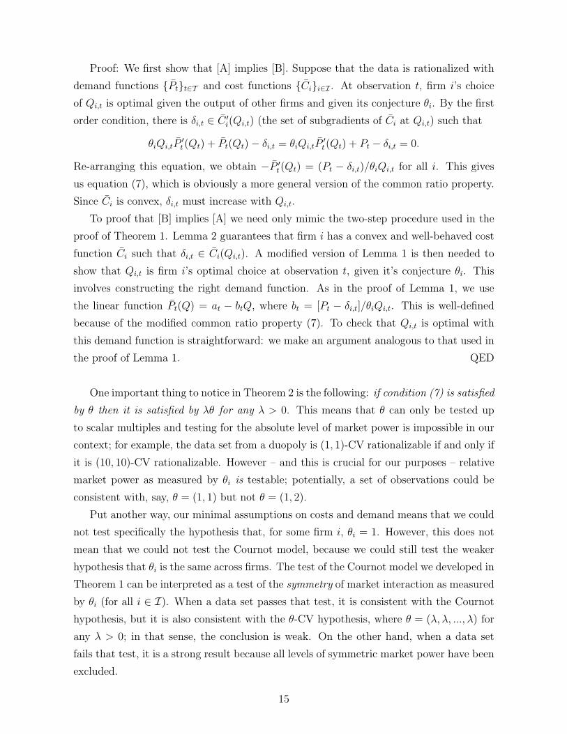
Proof: We first show that [A] implies [B]. Suppose that the data is rationalized with

demand functions {Pt}t∈T and cost functions {Ci}i∈I . At observation t, firm i’s choice

of Qi,t is optimal given the output of other firms and given its conjecture θi. By the first

order condition, there is δi,t ∈ C ′i(Qi,t) (the set of subgradients of Ci at Qi,t) such that

θiQi,tP′t(Qt) + Pt(Qt)− δi,t = θiQi,tP

′t(Qt) + Pt − δi,t = 0.

Re-arranging this equation, we obtain −P ′t(Qt) = (Pt − δi,t)/θiQi,t for all i. This gives

us equation (7), which is obviously a more general version of the common ratio property.

Since Ci is convex, δi,t must increase with Qi,t.

To proof that [B] implies [A] we need only mimic the two-step procedure used in the

proof of Theorem 1. Lemma 2 guarantees that firm i has a convex and well-behaved cost

function Ci such that δi,t ∈ Ci(Qi,t). A modified version of Lemma 1 is then needed to

show that Qi,t is firm i’s optimal choice at observation t, given it’s conjecture θi. This

involves constructing the right demand function. As in the proof of Lemma 1, we use

the linear function Pt(Q) = at − btQ, where bt = [Pt − δi,t]/θiQi,t. This is well-defined

because of the modified common ratio property (7). To check that Qi,t is optimal with

this demand function is straightforward: we make an argument analogous to that used in

the proof of Lemma 1. QED

One important thing to notice in Theorem 2 is the following: if condition (7) is satisfied

by θ then it is satisfied by λθ for any λ > 0. This means that θ can only be tested up

to scalar multiples and testing for the absolute level of market power is impossible in our

context; for example, the data set from a duopoly is (1, 1)-CV rationalizable if and only if

it is (10, 10)-CV rationalizable. However – and this is crucial for our purposes – relative

market power as measured by θi is testable; potentially, a set of observations could be

consistent with, say, θ = (1, 1) but not θ = (1, 2).

Put another way, our minimal assumptions on costs and demand means that we could

not test specifically the hypothesis that, for some firm i, θi = 1. However, this does not

mean that we could not test the Cournot model, because we could still test the weaker

hypothesis that θi is the same across firms. The test of the Cournot model we developed in

Theorem 1 can be interpreted as a test of the symmetry of market interaction as measured

by θi (for all i ∈ I). When a data set passes that test, it is consistent with the Cournot

hypothesis, but it is also consistent with the θ-CV hypothesis, where θ = (λ, λ, ..., λ) for

any λ > 0; in that sense, the conclusion is weak. On the other hand, when a data set

fails that test, it is a strong result because all levels of symmetric market power have been

excluded.

15

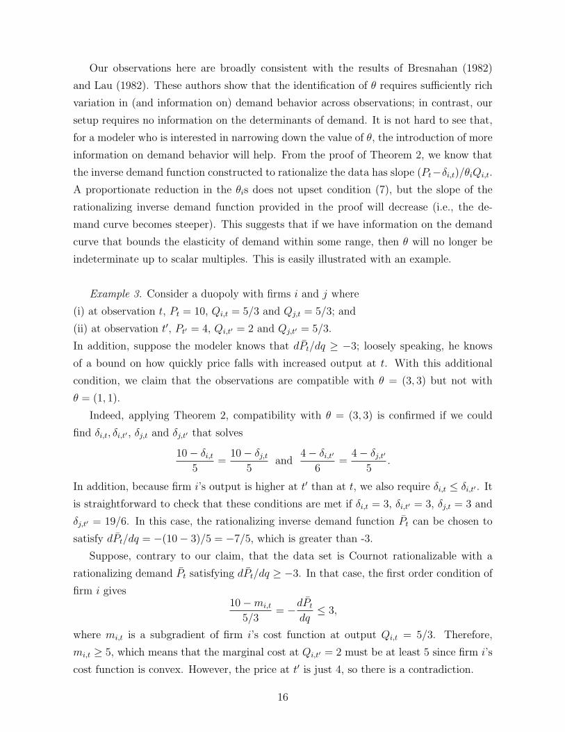
Our observations here are broadly consistent with the results of Bresnahan (1982)

and Lau (1982). These authors show that the identification of θ requires sufficiently rich

variation in (and information on) demand behavior across observations; in contrast, our

setup requires no information on the determinants of demand. It is not hard to see that,

for a modeler who is interested in narrowing down the value of θ, the introduction of more

information on demand behavior will help. From the proof of Theorem 2, we know that

the inverse demand function constructed to rationalize the data has slope (Pt−δi,t)/θiQi,t.

A proportionate reduction in the θis does not upset condition (7), but the slope of the

rationalizing inverse demand function provided in the proof will decrease (i.e., the de-

mand curve becomes steeper). This suggests that if we have information on the demand

curve that bounds the elasticity of demand within some range, then θ will no longer be

indeterminate up to scalar multiples. This is easily illustrated with an example.

Example 3. Consider a duopoly with firms i and j where

(i) at observation t, Pt = 10, Qi,t = 5/3 and Qj,t = 5/3; and

(ii) at observation t′, Pt′ = 4, Qi,t′ = 2 and Qj,t′ = 5/3.

In addition, suppose the modeler knows that dPt/dq ≥ −3; loosely speaking, he knows

of a bound on how quickly price falls with increased output at t. With this additional

condition, we claim that the observations are compatible with θ = (3, 3) but not with

θ = (1, 1).

Indeed, applying Theorem 2, compatibility with θ = (3, 3) is confirmed if we could

find δi,t, δi,t′ , δj,t and δj,t′ that solves

10− δi,t5

=10− δj,t

5and

4− δi,t′6

=4− δj,t′

5.

In addition, because firm i’s output is higher at t′ than at t, we also require δi,t ≤ δi,t′ . It

is straightforward to check that these conditions are met if δi,t = 3, δi,t′ = 3, δj,t = 3 and

δj,t′ = 19/6. In this case, the rationalizing inverse demand function Pt can be chosen to

satisfy dPt/dq = −(10− 3)/5 = −7/5, which is greater than -3.

Suppose, contrary to our claim, that the data set is Cournot rationalizable with a

rationalizing demand Pt satisfying dPt/dq ≥ −3. In that case, the first order condition of

firm i gives10−mi,t

5/3= −dPt

dq≤ 3,

where mi,t is a subgradient of firm i’s cost function at output Qi,t = 5/3. Therefore,

mi,t ≥ 5, which means that the marginal cost at Qi,t′ = 2 must be at least 5 since firm i’s

cost function is convex. However, the price at t′ is just 4, so there is a contradiction.

16

More generally, it is clear that with this lower bound on the slope of the inverse

demand function, there is λ∗ such that the observations are (λ, λ)-CV rationalizable if

λ > λ∗ and not (λ, λ)-CV rationalizable if λ < λ∗. It is worth comparing this example

with Lau (1982), who showed that the identification of θ = (λ, λ) requires that demand

be drawn from at least a two-parameter family. Our bound on the slope of demand does

not permit identification as such, but it is enough to identify a range of values of λ that

is consistent with the data; in certain situations, this coarser information may be all that

(say) an industry regulator is interested in.

We now outline a test for collusion that encompasses Example 3. The modeler assumes

that the data set is generated by demand varying across observations, while cost functions

are fixed. In addition, the inverse demand functions are drawn from a specified family

P . Besides observing Pt and (Qi,t)t∈T at each t, the observer also observes an n-vector

of parameters z ∈ Z ⊂ Rn that has a known impact on the elasticity of demand. More

precisely, we associate to each observation (q, p, z) ∈ R++ × R++ × Z a set S(q, p, z) ⊂(−∞, 0). Having observed (q, p, z), the observer assumes that the demand can be any

function P drawn from P , satisfying P (q) = p and with P ′(q) ∈ S(q, p, z).

We assume that P is a flexible family of inverse demand functions, by which we mean

that the following holds: (i) every element in P is downward sloping and log-concave and

(ii) given any observation (q, p) ∈ R2++ and any negative slope η, there is an element in P

passing through (q, p) and with slope η at that point. One example is the family of linear

inverse demand functions, with a typical element of the form P (q) = a− bq (where a and

b are positive numbers). Another example is the family of exponential inverse demand

functions, where P (q) = Ae−Bq and A and B are positive scalars. Note that both families

are also log-concave over that part of the domain where the price is positive.

Theorem 3. Given the correspondence I and a flexible family P, the following statements

on {[Pt, (Qi,t)i∈I , zt]}t∈T (with Pt > 0 for all t) are equivalent.

[A] The set of observations is θ-CV rationalizable (for θ � 0) with convex cost func-

tions and with the rationalizing inverse demand functions Pt drawn from P and satisfying

P ′t(Qt) ∈ S(Qt, Pt, zt).

[B] There exists a set of positive real numbers {δi,t}(i,t)∈I×T that obey the generalized com-

mon ratio property (7) and, for each i, {δi,t}t∈T is increasing with Qi,t. Furthermore,

[Pt − δ1,t]/θ1Q1,t ∈ S(Qt, Pt, zt) for all t ∈ T .

We shall omit the proof of this result since it can be done by an obvious modification

of the proofs given in Theorems 1 and 2. One important thing to note is that in proving

17

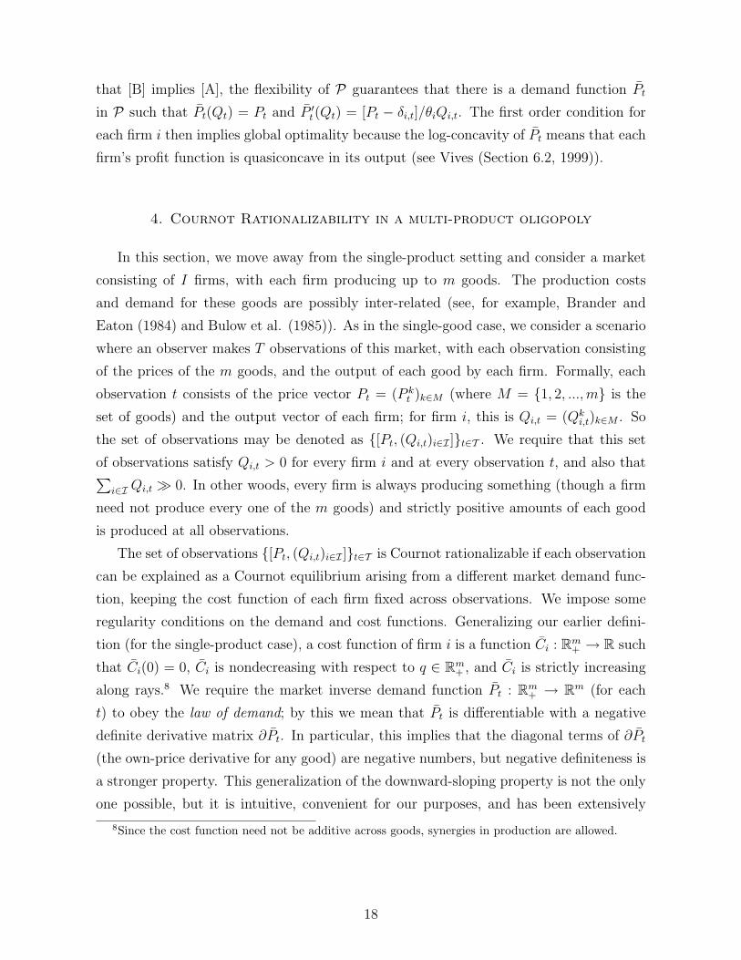
that [B] implies [A], the flexibility of P guarantees that there is a demand function Pt

in P such that Pt(Qt) = Pt and P ′t(Qt) = [Pt − δi,t]/θiQi,t. The first order condition for

each firm i then implies global optimality because the log-concavity of Pt means that each

firm’s profit function is quasiconcave in its output (see Vives (Section 6.2, 1999)).

4. Cournot Rationalizability in a multi-product oligopoly

In this section, we move away from the single-product setting and consider a market

consisting of I firms, with each firm producing up to m goods. The production costs

and demand for these goods are possibly inter-related (see, for example, Brander and

Eaton (1984) and Bulow et al. (1985)). As in the single-good case, we consider a scenario

where an observer makes T observations of this market, with each observation consisting

of the prices of the m goods, and the output of each good by each firm. Formally, each

observation t consists of the price vector Pt = (P kt )k∈M (where M = {1, 2, ...,m} is the

set of goods) and the output vector of each firm; for firm i, this is Qi,t = (Qki,t)k∈M . So

the set of observations may be denoted as {[Pt, (Qi,t)i∈I ]}t∈T . We require that this set

of observations satisfy Qi,t > 0 for every firm i and at every observation t, and also that∑i∈I Qi,t � 0. In other woods, every firm is always producing something (though a firm

need not produce every one of the m goods) and strictly positive amounts of each good

is produced at all observations.

The set of observations {[Pt, (Qi,t)i∈I ]}t∈T is Cournot rationalizable if each observation

can be explained as a Cournot equilibrium arising from a different market demand func-

tion, keeping the cost function of each firm fixed across observations. We impose some

regularity conditions on the demand and cost functions. Generalizing our earlier defini-

tion (for the single-product case), a cost function of firm i is a function Ci : Rm+ → R such

that Ci(0) = 0, Ci is nondecreasing with respect to q ∈ Rm+ , and Ci is strictly increasing

along rays.8 We require the market inverse demand function Pt : Rm+ → Rm (for each

t) to obey the law of demand; by this we mean that Pt is differentiable with a negative

definite derivative matrix ∂Pt. In particular, this implies that the diagonal terms of ∂Pt

(the own-price derivative for any good) are negative numbers, but negative definiteness is

a stronger property. This generalization of the downward-sloping property is not the only

one possible, but it is intuitive, convenient for our purposes, and has been extensively

8Since the cost function need not be additive across goods, synergies in production are allowed.

18

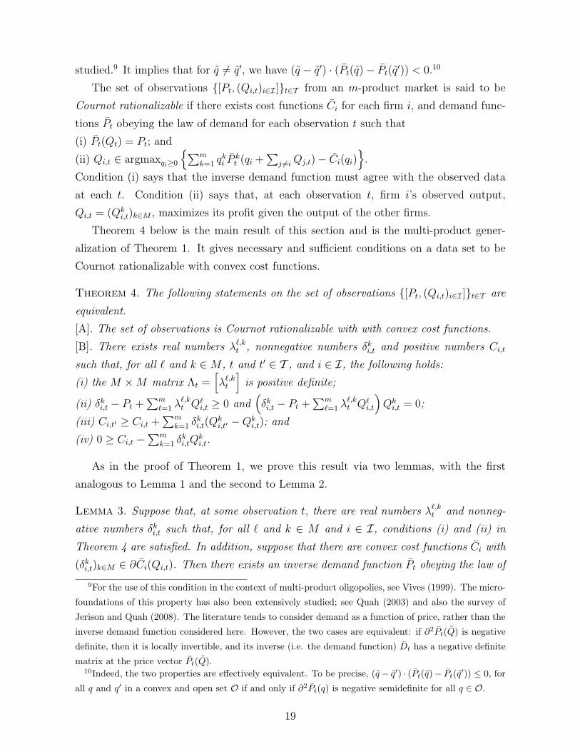
studied.9 It implies that for q 6= q′, we have (q − q′) · (Pt(q)− Pt(q′)) < 0.10

The set of observations {[Pt, (Qi,t)i∈I ]}t∈T from an m-product market is said to be

Cournot rationalizable if there exists cost functions Ci for each firm i, and demand func-

tions Pt obeying the law of demand for each observation t such that

(i) Pt(Qt) = Pt; and

(ii) Qi,t ∈ argmaxqi≥0

{∑mk=1 q

ki P

kt (qi +

∑j 6=iQj,t)− Ci(qi)

}.

Condition (i) says that the inverse demand function must agree with the observed data

at each t. Condition (ii) says that, at each observation t, firm i’s observed output,

Qi,t = (Qki,t)k∈M , maximizes its profit given the output of the other firms.

Theorem 4 below is the main result of this section and is the multi-product gener-

alization of Theorem 1. It gives necessary and sufficient conditions on a data set to be

Cournot rationalizable with convex cost functions.

Theorem 4. The following statements on the set of observations {[Pt, (Qi,t)i∈I ]}t∈T are

equivalent.

[A]. The set of observations is Cournot rationalizable with with convex cost functions.

[B]. There exists real numbers λ`,kt , nonnegative numbers δk

i,t and positive numbers Ci,t

such that, for all ` and k ∈M , t and t′ ∈ T , and i ∈ I, the following holds:

(i) the M ×M matrix Λt =[λ`,k

t

]is positive definite;

(ii) δki,t − Pt +

∑m`=1 λ

`,kt Q`

i,t ≥ 0 and(δki,t − Pt +

∑m`=1 λ

`,kt Q`

i,t

)Qk

i,t = 0;

(iii) Ci,t′ ≥ Ci,t +∑m

k=1 δki,t(Q

ki,t′ −Qk

i,t); and

(iv) 0 ≥ Ci,t −∑m

k=1 δki,tQ

ki,t.

As in the proof of Theorem 1, we prove this result via two lemmas, with the first

analogous to Lemma 1 and the second to Lemma 2.

Lemma 3. Suppose that, at some observation t, there are real numbers λ`,kt and nonneg-

ative numbers δki,t such that, for all ` and k ∈ M and i ∈ I, conditions (i) and (ii) in

Theorem 4 are satisfied. In addition, suppose that there are convex cost functions Ci with

(δki,t)k∈M ∈ ∂Ci(Qi,t). Then there exists an inverse demand function Pt obeying the law of

9For the use of this condition in the context of multi-product oligopolies, see Vives (1999). The micro-

foundations of this property has also been extensively studied; see Quah (2003) and also the survey of

Jerison and Quah (2008). The literature tends to consider demand as a function of price, rather than the

inverse demand function considered here. However, the two cases are equivalent: if ∂2Pt(Q) is negative

definite, then it is locally invertible, and its inverse (i.e. the demand function) Dt has a negative definite

matrix at the price vector Pt(Q).10Indeed, the two properties are effectively equivalent. To be precise, (q− q′) · (Pt(q)− Pt(q′)) ≤ 0, for

all q and q′ in a convex and open set O if and only if ∂2Pt(q) is negative semidefinite for all q ∈ O.

19

demand such that Pt(Qt) = Pt and, with each firm i having the cost function Ci, {Qi,t}i∈Iconstitutes a Cournot equilibrium.

Proof: We define the inverse demand function for good k by P kt (q) = ak

t −∑m

`=1 λk,`t q`

with akt chosen such that P k

t (Qt) = P kt . Firm i’s profit at observation t, given that firm

j 6= i is producing Qj,t is Πi,t(qi) = Ri,t(qi) − Ci(qi), where the revenue function Ri,t has

the form

Ri,t(qi) =m∑

`=1

q`i P

`t

(q`i +∑j 6=i

Q`j,t

).

Note that∂Ri,t

∂qki

(Qi,t) = P kt (Qt) +

m∑`=1

∂P `t

∂qk(Qt)Q

`i,t = P k

t −m∑

`=1

λ`,kt Q`

i,t. (8)

Since (δki,t)k∈M ∈ ∂Ci(Qi,t), condition (ii) gives the Kuhn-Tucker conditions for profit

maximization. These conditions are sufficient to guarantee that firm i’s choice is optimal

if Πi,t, is concave in qi. Given that Ci is a convex function, it suffices to check that

the Ri,t is concave in qi. It is straightforward to verify that, for all qi, the Hessian

∂2Ri,t(qi) = −ΛTt − Λt. Condition (i) guarantees that this matrix is negative definite, so

we conclude that Ri,t is concave. QED

Lemma 4. Suppose that for some firm i, there are nonnegative numbers δki,t and positive

numbers Ci,t such that, for all k ∈ M and t and t′ ∈ T , and i ∈ I, condition (iii)

and (iv) in Theorem 4 are satisfied. Then there exists a convex cost function such that

(δki,t)k∈M ∈ ∂Ci(Qi,t).

Proof: Let d = −maxt∈T {Ci,t−∑m

k=1 δki,tQ

ki,t}; by (iv), d ≥ 0. Given this, Ci,t = Ci,t+d

is a (strictly) positive number since Ci,t is a positive number. Define the function Ci by

Ci(q) = maxt∈T{Ci,t +

m∑k=1

δki,t(q

k −Qki,t)}. (9)

The function Ci has all but one of the conditions we require on the cost function. First,

notice that our choice of d guarantees that Ci(0) = 0. Since δki,t ≥ 0, the function Ci

is nondecreasing and since it is the upper envelope of linear functions, Ci is a convex

function. Condition (iii) implies that Ci(Qi,t) = Ci,t > 0 since

Ci,t ≥ Ci,s +m∑

k=1

δki,s(Q

ki,t −Qk

i,s) for all s ∈ T .

Therefore, (δki,t)k∈M ∈ ∂Ci(Qi,t).

20

However, Ci may not be strictly increasing along rays. To guarantee this property

we modify the function Ci in the following way. Choose a vector ε = (ε, ε, ..., ε) with

ε > 0 and sufficiently small so that Ci,t > ε · Qi,t for all t. Define the function Ci by

Ci(q) = max{Ci(q), ε · q}; Ci is a convex and nondecreasing function, with Ci(0) = 0

and Ci(Qi,t) = Ci,t. Locally at Qi,t, Ci and Ci are identical, so (δki,t)k∈M ∈ ∂Ci(Qi,t). In

addition, Ci is strictly increasing along rays. Suppose, to the contrary, that Ci is locally

constant along the ray through the point q = q. In that case, there exists s ∈ T such that

Ci,s +∑m

k=1 δki,s(λq

k−Qki,s) is constant and positive for all values of λ (and thus including

λ = 0), which is not possible since Ci(0) = 0. QED

Proof of Theorem 4: Suppose that [A] holds, so the data could be rationalized by

inverse demand functions P kt , for k ∈M and t ∈ T and cost functions Ci. We set

λ`,kt = −∂P

`t

∂qk(Qt).

Since (P kt )k∈M obeys the law of demand, Λt is positive definite as required by (i).

At observation t, the marginal revenue for firm i as it varies the output of good k is

P kt −

∑m`=1 λ

`,kt Q`

i,t (see (8)). Since Qi,t is optimal for firm i, there exists a vector (δki,t)k∈M

in ∂Ci(Qi,t) such that δki,t ≥ P k

t −∑m

`=1 λ`,kt Q`

i,t and with equality whenever Qki,t > 0 for

good k, so that (ii) holds. Since Ci is nondecreasing, we may choose the subgradient

(δki,t)k∈M to be a nonnegative vector.

Given that Ci is strictly increasing along rays and Qi,t > 0, we have Ci(Qi,t) > 0 for

all (i, t). Set Ci,t = Ci(Qi,t); since Ci is convex and (δki,t)k∈M is a subgradient, (iii) holds.

Finally, (iv) holds since Ci is convex and Ci(0) = 0. This completes our proof that [A]

implies [B].

The fact that [B] implies [A] follows immmediately from Lemmas 3 and 4. QED

Theorem 4 would be meaningless if in fact there are no observable restrictions in a

multi-product Cournot game. To remove this possibility, we now provide an example of

a data set that is not compatible with Cournot interaction.

Example 4. Consider an industry with two goods, 1 and 2. Observations taken from

two firms in this industry are as follows:

(i) at observation t, P 1t = 10, Q1

i,t = 13, Q2i,t = 12, Q1

j,t = 4, Q2j,t = 6.

(ii) at observation t′, P 1t′ = 1, P 2

t′ = 1, Q1j,t = 8 and Q2

j,t = 8.

Suppose that the observations at t constitutes a Cournot equilibrium. In that case,

21

the first order condition for firm i says that there is (δ1i,t, δ

2i,t) ∈ ∂Ci(Qi,t) such that

P 1t (Qt) +Q1

i,t

∂P 1t

∂q1

+Q2i,t

∂P 2t

∂q1

− δ1i,t = 0.

Similarly, the first order condition for firm j says that there is (δ1j,t, δ

2j,t) ∈ ∂Cj(Qj,t) such

that

P 1t (Qt) +Q1

j,t

∂P 1t

∂q1

+Q2j,t

∂P 2t

∂q1

− δ1j,t = 0.

Multiplying the first equation by Q2j,t and the second equation by Q2

i,t and taking the

difference between them, we obtain

(Q2j,t −Q2

i,t)P1t (Qt) +

[Q2

j,tQ1i,t −Q2

i,tQ1j,t

] ∂P 1t

∂q1

−Q2j,tδ

1i,t +Q2

i,tδ1j,t = 0. (10)

The significance of the numbers chosen for observation t is that they guarantee that

Q2j,t − Q2

i,t < 0 and Q2j,tQ

1i,t − Q2

i,tQ1j,t > 0. Note δ1

i,t ≥ 0 since firm i’s cost function is

nondecreasing and ∂P 1t /∂q1 < 0 because of the law of demand; therefore the second and

third terms on the left of equation (10) are both negative. Re-arranging that equation,

we obtain

δ1j,t ≥

(Q2i,t −Q2

j,t)

Q2i,t

P 1t (Qt) =

6

12· 10 = 5. (11)

In short, observation t provides us a with a lower bound on the marginal cost of firm j at

its observed output of (4, 6).

At observation t′, firm j’s output is (8, 8). The marginal cost of increasing output

from (4, 6) to (8, 8) is no smaller than the marginal cost of increasing output from (4, 6)

to (8, 6), which is in turn bounded below by 5×4 = 20 (because of (11) and the convexity

of Cj). So the total cost of producing (8, 8) is at least 20 but the total revenue of firm i at

observation t′ is just 16: firm i is better off choosing (0, 0) at observation t′. We conclude

that observations t and t′ cannot both be Cournot outcomes.

The multi-product setting of Theorem 4 raises a number of issues not present in the

single product setting of Theorem 1. We consider them in turn.

Like Theorem 1, Theorem 4 establishes an equivalence between Cournot rationaliz-

ability and the solution to a programming problem. However, the program in statement

[B] of Theorem 4 is not a linear program, because it requires checking that the matrix

Λ is positive definite (condition (i) in statement [B]). This condition is required for the

precise reason that we require the market demand function to obey the law of demand.

It is possible to replace the law of demand with a stronger condition that is easier to

22

check. For example, we could require the rationalizing inverse demand function Pt to

obey diagonal dominance with uniform weights; by this, we mean that

2∂P k

t

∂qk(q) +

∑` 6=k

∣∣∣∣∂P kt

∂q`(q) +

∂P `t

∂qk(q)

∣∣∣∣ < 0 for all q and for all k ∈M.

This intuitive condition says that own-price effects are larger than the sum of all cross-

price effects. If we impose this condition on the rationalizing demand system, then the

corresponding condition on δki,t (in place of condition (i) in [B]) is the following:

−2λk,kt +

∑6=k

∣∣∣λ`,kt + λk,`

t

∣∣∣ < 0 for all k ∈M ;11

note that this can condition can be equivalently stated as a set of linear conditions.

In certain contexts, the modeler may have specific information on cross price effects

which he would like to impose as conditions on the rationalizing demand system, on top

of those required by the law of demand or diagonal dominance. For example, it is possible

to interpret the different goods in this model as the same good sold in several distinct

and isolated markets; in other words, this multi-product oligopoly is an instance of third

degree price discrimination, with the same firms interacting in several markets. In that

case, it may be reasonable to require all cross price effects to equal zero, i.e., ∂P kt /∂q

` = 0

for all k 6= `. Correspondingly, one would have to impose the condition λ`,kt = 0 for all t

and whenever ` 6= k, in addition to the ones listed in statement [B] (of Theorem 4).

Similarly, the modeler may believe that the m goods are substitutes (∂P kt /∂q

` ≤ 0 for

all ` and k) or complements (∂P kt /∂q

` ≥ 0 for all ` 6= k). The corresponding conditions

are λ`,kt ≤ 0 for all ` and k and λ`,k

t ≥ 0 for all ` 6= k respectively.

If we impose the condition that all m goods are substitutes of each other then Cournot

rationalizability requires that all observed prices (P kt for all t and k) be non-negative.

Indeed, if P kt < 0 then any firm that is producing good k is strictly better off if it reduces

its output of k (which strictly increases revenue and at least weakly lowers costs). In the

case when the goods are not necessarily substitutes, the model allows for the possibility

that some observed prices are negative. In other words, firms can optimally pay for a

good to be consumed in order that it may raise the demand for some other good. It is

not hard to construct examples displaying this phenomenon.

11This property guarantees the positive definiteness of the symmetric matrix Λ+ΛT , which is equivalent

to the positive definiteness of Λ (see Mas-Colell et al. (Appendix M.D, 1995) for more on diagonal

dominance).

23

5. Convincing Cournot Rationalizability

In all our results so far, we have studied Cournot rationalizability when cost functions

display increasing marginal costs. This assumption on cost functions is of course ubiqui-

tous in both theoretical and empirical work; its great advantage is to ensure that the first

order conditions are not just necessary, but also sufficient, for optimality. Nonetheless,

in the context of oligopoly games, where increasing returns to scale may be present, it

is useful to have a test for the Cournot hypothesis that is not necessarily linked to firms

having increasing marginal costs.

In the one-good context, we could ask what conditions are needed for {[Pt, (Qi,t)i∈I ]}t∈Tto be Cournot rationalizable if we allow cost curves to be non-convex.12 The following

result says that Cournot competition imposes no restrictions on any generic set of ob-

servations {[Pt, (Qi,t)i∈I ]}t∈T ; by generic we mean that, for all i, Qi,t 6= Qi,t′ whenever

t 6= t′.

Proposition 2. Any generic set of observations {[Pt, (Qi,t)i∈I ]}t∈T is Cournot rational-

izable with firms having C2 cost functions.

To prove this result, and also to see how we could work around its seemingly negative

implication, it is useful to first consider a scenario where the observer has more information

at his disposal.

Suppose that, in addition to price and output, the observer also observes the total

cost incurred by each firm. Formally, the set of observations is {[Pt, (Qi,t)i∈I , (Ci,t)i∈I ]}t∈T ,

where Ci,t > 0 is the total cost incurred by firm i at output Qi,t > 0; we require Ci,t = Ci,t′

if Qi,t = Qi,t′ . We say that this set is Cournot rationalizable if there are downward sloping

(hence differentiable) inverse demand functions Pt (for all t ∈ T ) and cost functions Ci

(for each firm i ∈ I) such that Pt(Qt) = Pt, Ci(Qi,t) = Ci,t, and (Qi,t)i∈I is a Cournot

equilibrium when demand is Pt.

What restrictions does Cournot rationalizability impose on this data set? To answer

this question, we first need to introduce some notation. For each i and t, define the set

Li(t) = {t′ ∈ T : Qi,t′ < Qi,t} ∪ {0}.

Li(t) consists of those observations where firm i’s output is strictly lower thanQt, as well as

a fictitious observation 0, for which Q0 = 0 and Ci,0 = 0. We denote the observation where

firm i’s output is the lowest by t∗i . It follows that Li(t∗i ) = {0} whilst, for any t 6= t∗i , Li(t)

12Recall though, that our definition of cost curves require that they be continuous, strictly increasing,

and has no cost at output zero.

24

will contain t∗i , 0, and possibly other observations. We denote li(t) = argmaxt′∈Li(t)Qi,t′ ;

that is, li(t) is the set of observations corresponding to the highest output level strictly

below Qi,t.13 In a similar fashion, the observation with the highest output level for firm

i is denoted by t∗∗i . For t 6= t∗∗, the set of observations with outputs strictly higher than

t is denoted by Ui(t), with ui(t) = argmint′∈Ui(t)Qi,t′ , so ui(t) is the observation with the

lowest output level above Qi,t.

For any t in T , define dQi,t = Qi,t − Qi,li(t) and dCi,t = Ci,t − Ci,l(t). In words, dCi,t

is the extra cost incurred by firm i when it increases its output from Qi,l(t) to Qi,t. We

denote the average marginal cost over that output range by Mi,t = dCi,t/dQi,t.

We say that {Ci,t}(i,t)∈I×T obeys the discrete marginal property if for every i and t,

the following holds:

Ci,t − Ci,t′ < Pt(Qi,t −Qi,t′) for t′ ∈ Li(t). (12)

For any t′ ∈ Li(t), let Qi(t′, t) denote the set consisting of Qi,t and those observed output

levels of firm i strictly between Qi,t and Qi,t′ . Formally,

Qi(t′, t) = {Qi,s : s ∈ (Li(t) ∪ {t}) \ (Li(t

′) ∪ {t′}) }.

Since Ci,t−Ci,t′ =∑

Qi,s∈Qi(t′,t) Mi,s(Qi,s−Qi,l(s)) the discrete marginal property may also

be written as ∑Qi,s∈Qi(t′,t)

Mi,s(Qi,s −Qi,l(s)) < Pt(Qi,t −Qi,t′) for t′ ∈ Li(t). (13)

We claim that this property is necessary for Cournot rationalizability. Indeed, notice

that instead of producing at Qi,t, firm i could have chosen to produce at Qi,t′ for some

t′ ∈ Li(t) (that is, at a lower level of output). Given that Qi,t was chosen, the additional

cost incurred, which is Ci,t − Ci,t′ must be less than the additional revenue gained, and

the latter is bounded by Pt(Qi,t−Qi,t′) (because the demand curve is downward sloping).

The next result says that the discrete marginal property is both necessary and sufficient

for Cournot rationalizability.

Theorem 5. A generic set of observations {[Pt, (Qi,t)i∈I , (Ci,t)i∈I ]}t∈T is Cournot ratio-

nalizable with C2 cost functions if and only if it obeys the discrete marginal property.

The proof of this result requires the following lemma.

13In particular, li(t∗i ) = {0}. When the data set is generic, li(t) is always singleton; otherwise it could

have more than one element.

25

Lemma 5. Let {[Pt, (Qi,t)i∈I , (Ci,t)i∈I ]}t∈T be a generic set of observations obeying the

discrete marginal property and suppose that the positive numbers {δi,t}(i,t)∈I×T satisfy

0 < δi,t < Pt, for all (i, t), with δi,t = δi,t′ whenever Qi,t = Qi,t′. Then, there are C2 cost

functions Ci : R+ → R such that

(i) Ci(Qi,t) = Ci,t;

(ii) C ′i(Qi,t) = δi,t; and

(iii) for all qi in [0, Qi,t),

Ptqi − Ci(qi) < PtQi,t − Ci(Qi,t). (14)

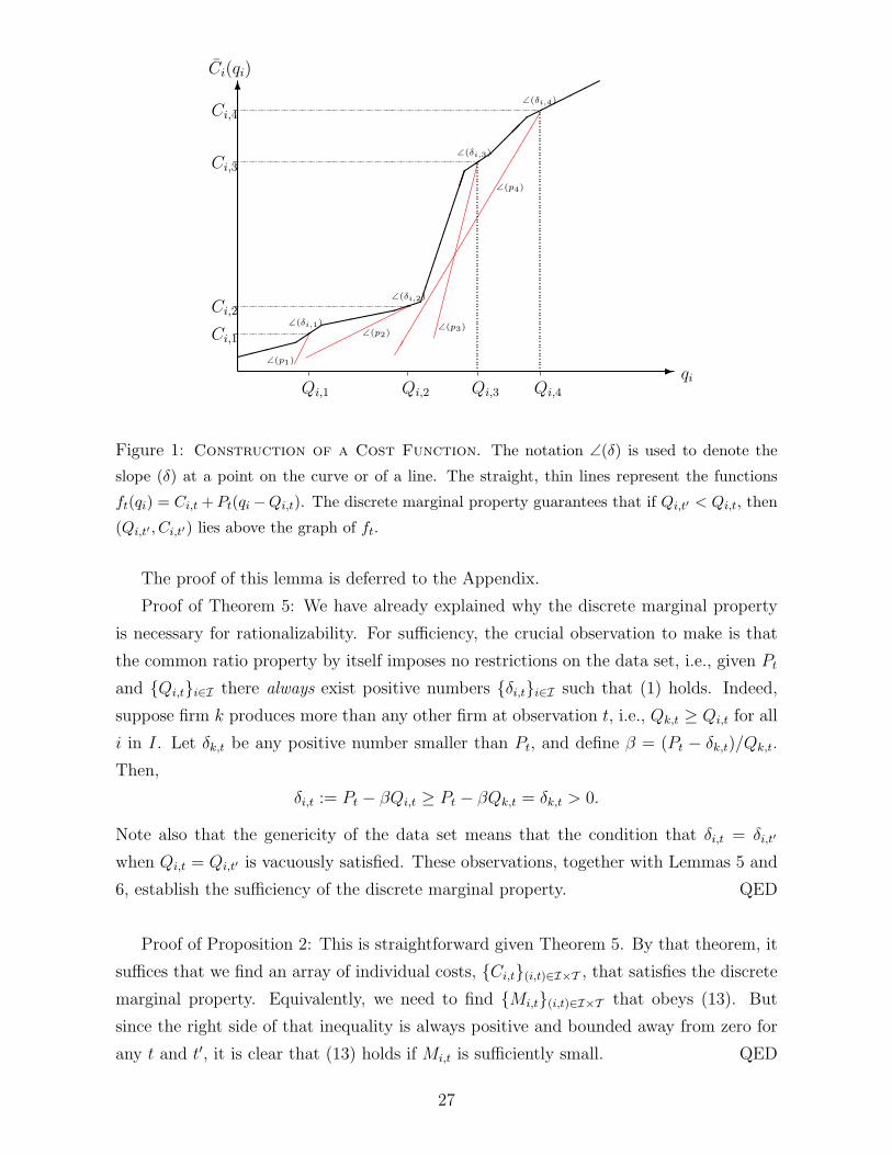
Proof: Note that the inequality (14) may be re-written as

Ci(qi) > Pt(qi −Qi,t) + Ci(Qi,t). (15)

The function ft(qi) = Pt(qi − Qi,t) + Ci,t, for qi in [0, Qi,t), is represented by a line with

slope Pt passing through the point (Qi,t, Ci,t) – see Figure 1. Condition M guarantees that

for t′ in Li(t), (Qi,t′ , Ci,t′) lies above the line ft. We require a cost function that satisfies

(15). One such function is the one given by the linear interpolation of all the points

(Qi,t, Ci,t), since its graph stays above every one of the lines representing the functions ft.

This cost function can in turn be replaced by a C2 function where the derivative at Qi,t

is δi,t, since δi,t < Pt and the latter is the slope of ft. QED

This lemma says that there is a cost function for firm i that (i) agrees with the observed

values of firm costs, (ii) has marginal cost agreeing with specified values at the observed

output levels, and (iii) guarantees that q = Qi,t is the optimal output level for firm i if

the inverse demand function at t is Pt(q) = Pt for q ≤ Qt and Pt(q) = 0 for q > Qt. So

we have almost proved Theorem 5, and we fall a bit short only because the rationalizing

demand function Pt we just provided is not differentiable or downward sloping in our

sense. However, as we show in the next result, it is always possible to replace Pt with

a downward sloping inverse demand function Pt that preserves the optimality of firm i’s

output choice.

Lemma 6. Let {δi,t}(i,t)∈I×T be a set of positive numbers, with δi,t = δi,t′ whenever Qi,t =

Qi,t′, satisfying the common ratio property (1) and suppose that the C2 cost functions

Ci : R+ → R satisfy properties (i)-(iii) in Lemma 5. Then there are downward sloping

inverse demand functions Pt : R+ → R such that, Pt(∑

i∈I Qi,t) = Pt and, for every i,

argmaxqi≥0

{qiPt(qi +

∑j 6=i

Qj,t)− Ci(qi)

}= Qi,t.

26

-

6

������

�������������������

���

��

�����

��

������������

��

��

��

��

��

��

��

��

�

qi

Ci(qi)

Qi,1 Qi,2 Qi,3 Qi,4

Ci,1

Ci,2

Ci,3

Ci,4

∠(δi,1)

∠(δi,2)

∠(δi,3)

∠(δi,4)

∠(p1)

∠(p2)∠(p3)

∠(p4)

Figure 1: Construction of a Cost Function. The notation ∠(δ) is used to denote the

slope (δ) at a point on the curve or of a line. The straight, thin lines represent the functions

ft(qi) = Ci,t +Pt(qi −Qi,t). The discrete marginal property guarantees that if Qi,t′ < Qi,t, then

(Qi,t′ , Ci,t′) lies above the graph of ft.

The proof of this lemma is deferred to the Appendix.

Proof of Theorem 5: We have already explained why the discrete marginal property

is necessary for rationalizability. For sufficiency, the crucial observation to make is that

the common ratio property by itself imposes no restrictions on the data set, i.e., given Pt

and {Qi,t}i∈I there always exist positive numbers {δi,t}i∈I such that (1) holds. Indeed,

suppose firm k produces more than any other firm at observation t, i.e., Qk,t ≥ Qi,t for all

i in I. Let δk,t be any positive number smaller than Pt, and define β = (Pt − δk,t)/Qk,t.

Then,

δi,t := Pt − βQi,t ≥ Pt − βQk,t = δk,t > 0.

Note also that the genericity of the data set means that the condition that δi,t = δi,t′

when Qi,t = Qi,t′ is vacuously satisfied. These observations, together with Lemmas 5 and

6, establish the sufficiency of the discrete marginal property. QED

Proof of Proposition 2: This is straightforward given Theorem 5. By that theorem, it

suffices that we find an array of individual costs, {Ci,t}(i,t)∈I×T , that satisfies the discrete

marginal property. Equivalently, we need to find {Mi,t}(i,t)∈I×T that obeys (13). But

since the right side of that inequality is always positive and bounded away from zero for

any t and t′, it is clear that (13) holds if Mi,t is sufficiently small. QED

27

When costs are not directly observable, Cournot rationalizabilty requires that there

be {δi,t}(i,t)∈I×T satisfying the common ratio property and {Ci,t}(i,t)∈I×T (equivalently,

{Mi,t}(i,t)∈I×T ) obeying the discrete marginal property. The former is a condition on the

infinitesimal marginal costs of each firm while the latter is a condition on the average

marginal costs of each firm. Both conditions in fact impose no restrictions, in the sense

that, given any data set, it is always possible to find δi,t and Mi,t that satisfy those

conditions.

What makes Proposition 2 possible – and also what makes its seemingly negative

conclusion less than persuasive – is that there need be no link between δi,t and Mi,t. In

fact the proof relies crucially on the freedom to choose Mi,t to be arbitrarily small, so that

it could be considerable smaller than both C ′i(Qi,l(t)) = δi,l(t) and C ′i(Qi,t) = δi,t. Since

we impose no restrictions on C ′i (apart from it being a continuous function of output),

this is formally permissible, but a rationalizing cost function for firm i that requires the

modeler (or his audience) to believe in such a disconnection between infinitesimal and

average marginal costs is not persuasive.14

One way of avoiding such ill-behaved marginal cost functions is to take as the marginal

cost function between Qi,t and Qi,li(t) the linear interpolation of the hypothesized marginal

costs at those two outputs, i.e, the marginal cost curve is the straight line joining (Qi,l(t), δi,l(t))

and (Qi,t, δi,t). In that case, the average marginal cost between those two outputs is ex-

actly [δi,li(t) + δi,t]/2. We wish to have more flexibility in our choice of the marginal cost

function than simply taking a linear interpolation, but what we could require is that the

rationalizing cost function’s average marginal cost between those two outputs is at least

[δi,li(t) + δi,t]/2.

Formally, a C2 cost function Ci for firm i is said to be convincing or to satisfy the

convincing criterion (given observed output {Qi,t}t∈T ) if

Ci(Qi,t)− Ci(Qi,li(t))

Qi,t −Qi,l(t)

≥ 1

2

[C ′i(Qi,l(t)) + C ′i(Qi,t)

]for all t 6= t∗i . (16)

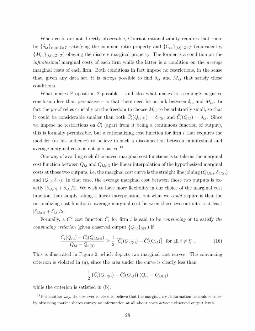
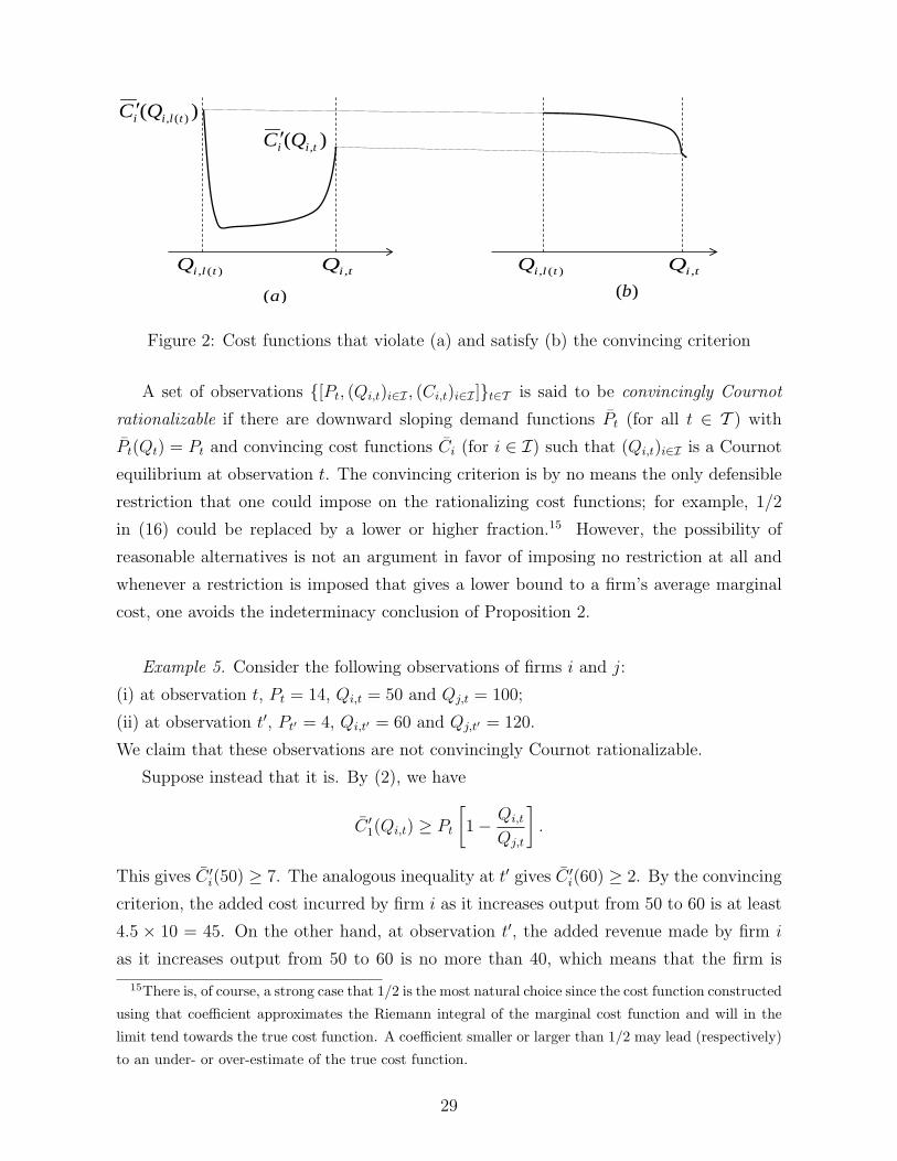
This is illustrated in Figure 2, which depicts two marginal cost curves. The convincing

criterion is violated in (a), since the area under the curve is clearly less than

1

2

(C ′i(Qi,l(t)) + C ′i(Qi,t)

)(Qi,t −Qi,l(t))

while the criterion is satisfied in (b).

14Put another way, the observer is asked to believe that the marginal cost information he could surmise

by observing market shares convey no information at all about costs between observed output levels.

28

tiQ ,)(, tliQ )(, tliQ

)( )(, tlii QC ′)( ,tii QC ′

tiQ ,

)(a )(b

Figure 2: Cost functions that violate (a) and satisfy (b) the convincing criterion

A set of observations {[Pt, (Qi,t)i∈I , (Ci,t)i∈I ]}t∈T is said to be convincingly Cournot

rationalizable if there are downward sloping demand functions Pt (for all t ∈ T ) with

Pt(Qt) = Pt and convincing cost functions Ci (for i ∈ I) such that (Qi,t)i∈I is a Cournot

equilibrium at observation t. The convincing criterion is by no means the only defensible

restriction that one could impose on the rationalizing cost functions; for example, 1/2

in (16) could be replaced by a lower or higher fraction.15 However, the possibility of

reasonable alternatives is not an argument in favor of imposing no restriction at all and

whenever a restriction is imposed that gives a lower bound to a firm’s average marginal

cost, one avoids the indeterminacy conclusion of Proposition 2.

Example 5. Consider the following observations of firms i and j:

(i) at observation t, Pt = 14, Qi,t = 50 and Qj,t = 100;

(ii) at observation t′, Pt′ = 4, Qi,t′ = 60 and Qj,t′ = 120.

We claim that these observations are not convincingly Cournot rationalizable.

Suppose instead that it is. By (2), we have

C ′1(Qi,t) ≥ Pt

[1− Qi,t

Qj,t

].

This gives C ′i(50) ≥ 7. The analogous inequality at t′ gives C ′i(60) ≥ 2. By the convincing

criterion, the added cost incurred by firm i as it increases output from 50 to 60 is at least

4.5 × 10 = 45. On the other hand, at observation t′, the added revenue made by firm i

as it increases output from 50 to 60 is no more than 40, which means that the firm is

15There is, of course, a strong case that 1/2 is the most natural choice since the cost function constructed

using that coefficient approximates the Riemann integral of the marginal cost function and will in the

limit tend towards the true cost function. A coefficient smaller or larger than 1/2 may lead (respectively)

to an under- or over-estimate of the true cost function.

29

better off producing at 50 rather than 60 at t′. We conclude that these observations are

not convincingly rationalizable.

Our final result sets out the necessary and sufficient conditions for a set of observations

to be convincingly Cournot rationalizable. Note that these conditions take the form of a

linear program so its implementation is not typically a complex issue.

Theorem 6. A set of observations {[Pt, (Qi,t)i∈I ]}t∈T is convincingly Cournot rational-

izable if, and only if, the following conditions are satisfied:

(a) there are positive scalars {δi,t}(i,t)∈I×T , with δi,t = δi,t′ if Qi,t = Qi,t′, that has the

common ratio property;

(b) there are positive scalars {∆i,t}(i,t)∈I×T , with ∆i,t = ∆i,t′ if Qi,t = Qi,t′, that has the

discrete marginal property, i.e.,∑Qi,s∈Q(t′,t)

∆i,s

(Qi,s −Qi,l(s)

)< Pt(Qt −Qt′) for all t′ ∈ Li(t); and (17)

(c) for all i and t 6= t∗i ,

∆i,t ≥1

2

[δi,li(t) + δi,t

]. (18)

Proof: To see that these conditions are necessary, set δi,t = C ′i(Qi,t) and ∆i,t =

[Ci(Qi,t) − Ci(Qi,li(t))]/[Qi,t − Qi,li(t)]. Then (c) is just the convincing criterion on the

cost functions, (a) follows from the first order condition at the equilibrium and we have

already explained why (b) (see the discussion following (13)).

For the sufficiency of the conditions, set

Ci,t =∑

Qi,s∈Qi(t∗i ,t)

∆i,s(Qi,s −Qi,l(s)) ;

then (17) guarantees that the data set {[Pt, (Qi,t)i∈I , (Ci,t)i∈I ]}t∈T obeys the discrete

marginal property (see (12) and (13)). Lemmas 5 and 6 then guarantee the existence

of Pt and Ci with the desired properties. In particular, Ci(Qi,t) = Ci,t, C′i(Qi,t) = δi,t

and the average marginal cost between Qi,l(t) and Qi,t, is ∆i,t, so that Ci satisfies the

convincing criterion because of (18). QED

Corollary 1 says that there is a Cournot rationalization with C1 convex cost curves if

the common ratio property holds and δi,t is finely increasing with Qi,t. Note that the latter

condition guarantees the existence ∆i,t obeying (b) and (c) in Theorem 6: set ∆i,t = δi,t

and it is clear that (17) and (18) are satisfied. So Theorem 6 is certainly consistent with

30

Corollary 1. Of course, the interest of this result lies precisely in the fact that it poten-

tially allows for cases where δi,t is not increasing with Qi,t.

6. Allowing for Noisy Data

Revealed preference tests by their very nature are exact. Errors in the observed data

could lead to a potential false rejection by the test even if the errors are small. Put

differently, one might be concerned that our tests might reject the data due to small

measurement errors even though underlying true data is consistent with Cournot behavior.

An insight by Varian (1985) allows us to deal with such issues. In this section, we briefly

describe how his approach can be adapted to our tests.

Once again, consider the case of single product where firms have convex cost functions.

We denote the set of data sets which are Cournot rationalizable with convex cost functions

by D. Formally,

D =

{{[Pt, (Qi,t)i∈I ]}t∈T : {[Pt, (Qi,t)i∈I ]}t∈T is Cournot rationalizable

with convex cost functions

}.

Assume that we are given an observed data set {[Pt, (Qi,t)i∈I ]}t∈T that is not Cournot

rationalizable with convex cost functions, so {[Pt, (Qi,t)i∈I ]}t∈T /∈ D. Suppose that this

data set has been contaminated with measurement error. In other words, the “true” data

set is given by

{[Pt + εPt , (Qi,t + εQ

i,t)i∈I ]}t∈T ,

where the error terms Ξ ={εP

t , (εQi,t)i∈I

}t∈T

are assumed to be classical with variance σ2.

Consider now the null hypothesis that the true data set is Cournot rationalizable with

convex cost functions. A test statistic for this null hypothesis can now be based on the

loss function

L =Ξ

σ2,

where Ξ is the vector formed by concatenating the errors in the set Ξ. Since the errors are

normally distributed the test statistic L will have a chi-squared distribution with degrees

of freedom equal to the number of data points. Hence, we can find critical values for any

desired level of significance and reject the null hypothesis if the test statistic is great than

the critical value.

31

Since the errors are not observed, we can compute the test statistic by solving the

following optimization problem:

minΞ

{Ξ

σ2

},

subject to {[Pt + εPt , (Qi,t + εQ

i,t)i∈I ]}t∈T ∈ D.

This problem essentially involves finding the minimum perturbation to the observed data

so that the perturbed data is Cournot rationalizable. The above constraint is simply the

set of inequalities and equalities imposed in Theorem 1 and as a result it is a well defined

numerical optimization problem.

It is worth pointing out that the variance of the measurement error is typically un-

known. Varian (1985) suggests that estimates of the variance can be obtained from

parametric or nonparametric fits of the data, from knowledge of how the variables were

actually measured or from other data sources. Alternatively, he suggests computing how

large the variance would need to be in order for the null hypothesis to be accepted and

comparing this value to our prior opinions. If it is much smaller than our prior opinions

regarding the precision with which the data has been measured, we may be compelled to

accept the null.

Of course, the above procedure can be applied to all the generalizations of the basic

result. We can consider the set D to be the set of data sets which are Cournot ratio-

nalizable with cost shifters, θ − CV rationalizable, Cournot rationalizable with multiple

products or convincing Cournot rationalizable.

7. Application: The world market for crude oil

Petroleum accounts for more than one third of global energy consumption, and in

April 2009 world oil production was more than 72 million barrels per day (Monthly Energy

Review (MER), 2009). Accounting for roughly one third of global oil production, OPEC

is a dominant player in the international oil market. OPEC was founded in 1960 and

exists, in its own words, “to co-ordinate and unify petroleum policies among Member

Countries, in order to secure fair and stable prices for petroleum producers; an efficient,

economic and regular supply of petroleum to consuming nations; and a fair return on

capital to those investing in the industry.” OPEC rose to prominence during the energy

crises of the 1970s for its embargo in response to Western support of Israel during the 1973

Yom Kippur War. Since the start of the 1980s, with the abolition of US price controls

and increased production by the rest of the world, OPEC’s influence on oil prices has

declined. Beginning in 1982, OPEC began to allocate production quotas to its members,

32

replacing a system of posted prices. This has not, however, permitted OPEC to dictate

world prices, since the majority the world’s oil is produced by non-members and the only

sanction available to police its members is Saudi Arabia’s spare capacity.

OPEC’s stated aims are effectively those of a cartel, but its ability to set world oil

prices is questionable. Hence, a large literature has emerged that attempts to model

its actions and to test whether these models fit its observed behavior. For the most

part, the literature suggests that OPEC is a “weakly functioning cartel” of some sort,

and is not “competitive” in either the price-taking or non-cooperative Cournot senses –

see, for example, Alhajji and Huettner (2000), Almoguera and Herrera (2007), Dahl and

Yucel (1991), Griffin and Neilson (1994), or Smith (2005). Many of these tests rely on

parametric assumptions about the functional forms taken by market demand, countries’

objective functions and production costs. Typically, they also require that factors shifting

the cost and inverse demand functions be observed, and rely on constructed proxies such as

estimates of countries’ extraction costs, the presence of US price controls, and involvement

of an OPEC member in a war. Given the ambitious questions they are trying to answer,

this seems unavoidable.

Our objective is more modest and more specific. All we wish to do is to use the re-

sults developed in the previous sections to test whether the behavior of the oil-producing

countries is consistent with the Cournot model or, more generally (given the discussion

in Section 3), any symmetric CV model. Our tests make use of very few ancillary as-

sumptions, giving, so to speak, the greatest benefit of the doubt to the hypothesis, by

allowing for a very large class of cost functions and by not making any assumptions at all

about the evolution of demand (apart from the assumption that it is downward sloping

with respect to output). In spite of this apparent permissiveness, our tests can reject the

restrictions of the Cournot model in real world data.

Two sources of data are used for this study. The first is the Monthly Energy Review

(MER), published by the US Energy Information Administration. This provides full-

precision series of monthly crude oil production in thousands of barrels per day by the

twelve current OPEC members (Algeria, Angola, Ecuador, Iran, Iraq, Kuwait, Libya,

Nigeria, Qatar, Saudi Arabia, the United Arab Emirates, and Venezuela) and seven non-

members (Canada, China, Egypt, Mexico, Norway, the United States, and the United

Kingdom).16 This series also contains total world output. The data are available from

16Russia and the former Soviet Union are not used here, because the two are not comparable units.

Although the composition of OPEC has changed over the course of the data (Ecuador left in 1994 and

returned in 2007, Gabon left in 1995, Angola joined in 2007, and Indonesia left in 2007), the overall

33

January 1973 until April 2009, giving a total length of T = 436 months and M×T = 8248

country-month observations. There are only seven instances in the data in which an

individual country’s monthly production is zero,17 and so false acceptances and rejections

of the test due to violation of this assumption will be small in number. The second source

of data is a series of oil prices published by the St. Louis Federal Reserve, in dollars

per barrel. This series is deflated by the monthly consumer price index reported by the

Bureau of Labor Statistics, so that prices are in 2009 US dollars. Since the time windows

over which Cournot behavior is tested are short (twelve months or less), the adjustment

for inflation should not matter to the results.18

Each test consists of using a linear programming algorithm to find whether there exists

a solution to the specified linear program. If a solution exists, this subset of the data can

be rationalized within the Cournot model, i.e. Cournot behavior by these M countries is

supported by the data during the period tested. Clearly, as M and W increase, it is more

likely that at least one country is not behaving optimally in at least one period, and so

it is more likely that it will not be possible to satisfy the set of inequalities. Rather than

performing a single test for whether the entire data series can be rationalized, we select

a number of countries M , and then test whether the data for each of the(

MM

)possible

combinations of countries in each of the T+1−W periods of length W can be rationalized.

We then report the percentage of these(

MM

)×(T +1−W ) cases in which optimal behavior

is rejected. The time windows selected are short; W is either 3 months, 6 months, or 12

months. This is in keeping with the assumption that cost functions do not change over

the period of the test. If a test is able to reject for a small amount of data (for example,

three countries over three months), it demonstrates that, despite the generality of the

non-parametric framework, the test has sufficient power to detect non-optimal behavior

in real data.

We use the linear program specified in Theorem 1 to test whether the data sets are

Cournot rationalizable with convex cost curves. Table 1 presents the percentage of cases

(in the sense explained in the Notes below the table) for which the data is not Cournot

rationalizable with convex costs over groups of 2, 3, 6 and 12 OPEC countries within

windows of 3, 6, and 12 months. The results are unambiguous – once there are more than

a handful of observations used for the test, the behavior of OPEC members cannot be

pattern of rejecting Cournot behavior below does not depend on what countries are considered to be part

of OPEC. Reported tests consider groups of 2, 3, 6, and 12 member states; these overwhelmingly reject

Cournot behavior for almost all country groups in periods longer than a few months.17Ecuador, April, 1987; Iraq, February and March, 1991; Kuwait, February through April, 1991.18The rejection rates reported below are similar with nominal price series.

34

Table 1: Rejection rates with convex cost functions

OPEC sample

Number of Countries

2 3 6 12

3 Months 0.28 0.54 0.89 1.00

Window 6 Months 0.65 0.89 1.00 1.00

12 Months 0.90 0.99 1.00 1.00

Non-OPEC sample

Number of Countries

2 3 6 7

3 Months 0.44 0.75 0.99 1.00

Window 6 Months 0.83 0.98 1.00 1.00

12 Months 0.96 1.00 1.00 1.00Notes: The rejection rate reported is the proportion of cases that were rejected. For example, there

are 436 + 1 − 3 = 434 three month periods in the data. There are 66 possible combinations of two out

of twelve OPEC members. The entry for two countries and three months, then, reports that out of the

434 × 66 = 28, 644 possible tests of two OPEC members over three months, 8138, or 28% could not be

rationalized.

explained by the Cournot model with convex costs. For nearly 90% of six-month periods

with three countries, the test rejects optimal behavior. Once six countries are included,

fewer than one six-month case in ten thousand can be rationalized. The same test was

performed for the non-OPEC countries (see Table 1). Once again the results are strongly

against the Cournot model. For almost all six month periods, when at least three countries

are considered, the data cannot be rationalized by the Cournot model with convex costs.

It is, in principle, possible that the tests reported in Table 1 rejected the Cournot

hypothesis because the convexity of the cost functions is too strong an assumption. To

address this potential problem, tests for convincing Cournot rationalizability (which al-

lows for non-convex costs) using the linear program specified in Theorem 6 were also

carried out. These are reported in Table 2. Given the very permissive setup, one may

expect the test to have little power, but that is not the case. Rejection rates for the

countries in OPEC exceed 50% with 3 countries and 6 observations. In the case of the

non-OPEC countries the drop in the rejection rate is sharper and the picture becomes

mixed, with rejection exceeding 50% only with 6 countries and 6 observations.

35

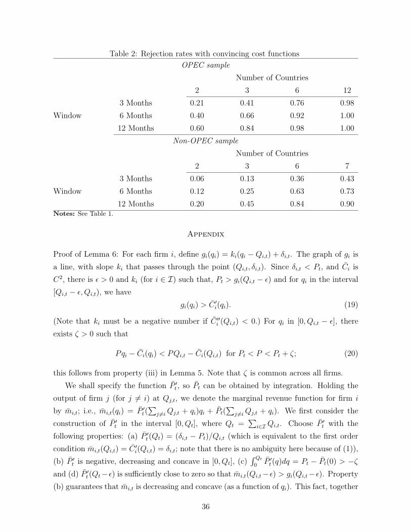
Table 2: Rejection rates with convincing cost functions

OPEC sample

Number of Countries

2 3 6 12

3 Months 0.21 0.41 0.76 0.98

Window 6 Months 0.40 0.66 0.92 1.00

12 Months 0.60 0.84 0.98 1.00

Non-OPEC sample

Number of Countries

2 3 6 7

3 Months 0.06 0.13 0.36 0.43

Window 6 Months 0.12 0.25 0.63 0.73

12 Months 0.20 0.45 0.84 0.90Notes: See Table 1.

Appendix

Proof of Lemma 6: For each firm i, define gi(qi) = ki(qi − Qi,t) + δi,t. The graph of gi is

a line, with slope ki that passes through the point (Qi,t, δi,t). Since δi,t < Pt, and Ci is

C2, there is ε > 0 and ki (for i ∈ I) such that, Pt > gi(Qi,t − ε) and for qi in the interval

[Qi,t − ε, Qi,t), we have

gi(qi) > C ′i(qi). (19)

(Note that ki must be a negative number if C ′′i (Qi,t) < 0.) For qi in [0, Qi,t − ε], there

exists ζ > 0 such that

Pqi − Ci(qi) < PQi,t − Ci(Qi,t) for Pt < P < Pt + ζ; (20)

this follows from property (iii) in Lemma 5. Note that ζ is common across all firms.

We shall specify the function P ′t , so Pt can be obtained by integration. Holding the

output of firm j (for j 6= i) at Qj,t, we denote the marginal revenue function for firm i

by mi,t; i.e., mi,t(qi) = P ′t(∑

j 6=iQj,t + qi)qi + Pt(∑

j 6=iQj,t + qi). We first consider the

construction of P ′t in the interval [0, Qt], where Qt =∑

i∈I Qi,t. Choose P ′t with the

following properties: (a) P ′t(Qt) = (δi,t − Pt)/Qi,t (which is equivalent to the first order

condition mi,t(Qi,t) = C ′i(Qi,t) = δi,t; note that there is no ambiguity here because of (1)),

(b) P ′t is negative, decreasing and concave in [0, Qt], (c)∫ Qt

0P ′t(q)dq = Pt − Pt(0) > −ζ

and (d) P ′t(Qt− ε) is sufficiently close to zero so that mi,t(Qi,t− ε) > gi(Qi,t− ε). Property

(b) guarantees that mi,t is decreasing and concave (as a function of qi). This fact, together

36

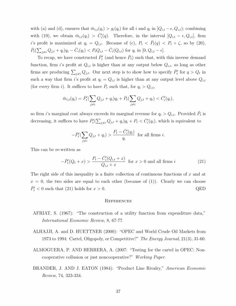
with (a) and (d), ensures that mi,t(qi) > gi(qi) for all i and qi in [Qi,t− ε, Qi,t); combining

with (19), we obtain mi,t(qi) > C ′i(q). Therefore, in the interval [Qi,t − ε, Qi,t], firm

i’s profit is maximized at qi = Qi,t. Because of (c), Pt < Pt(q) < Pt + ζ, so by (20),

Pt(∑

j 6=iQj,t + qi)qi − Ci(qi) < PtQi,t − Ci(Qi,t) for qi in [0, Qi,t − ε].To recap, we have constructed P ′t (and hence Pt) such that, with this inverse demand

function, firm i’s profit at Qi,t is higher than at any output below Qi,t, so long as other

firms are producing∑

j 6=iQj,t. Our next step is to show how to specify P ′t for q > Qt in

such a way that firm i’s profit at qi = Qi,t is higher than at any output level above Qi,t

(for every firm i). It suffices to have Pt such that, for qi > Qi,t,

mi,t(qi) = P ′t(∑j 6=i

Qj,t + qi)qi + Pt(∑j 6=i

Qj,t + qi) < C ′i(qi),

so firm i’s marginal cost always exceeds its marginal revenue for qi > Qi,t. Provided Pt is

decreasing, it suffices to have P ′t(∑

j 6=iQj,t + qi)qi + Pt < C ′i(qi), which is equivalent to

−P ′t(∑j 6=i

Qj,t + qi) >Pt − C ′i(qi)

qifor all firms i.

This can be re-written as

−P ′t(Qt + x) >Pt − C ′i(Qi,t + x)

Qi,t + xfor x > 0 and all firms i (21)

The right side of this inequality is a finite collection of continuous functions of x and at

x = 0, the two sides are equal to each other (because of (1)). Clearly we can choose

P ′t < 0 such that (21) holds for x > 0. QED

References

AFRIAT, S. (1967): “The construction of a utility function from expenditure data,”

International Economic Review, 8, 67-77.

ALHAJJI, A. and D. HUETTNER (2000): “OPEC and World Crude Oil Markets from

1973 to 1994: Cartel, Oligopoly, or Competitive?” The Energy Journal, 21(3), 31-60.

ALMOGUERA, P. AND HERRERA, A. (2007: “Testing for the cartel in OPEC: Non-

cooperative collusion or just noncooperative?” Working Paper.

BRANDER, J. AND J. EATON (1984): “Product Line Rivalry,” American Economic

Review, 74, 323-334.

37

BRESNAHAN, T. (1982): “The oligopoly solution concept is identified,” Economics

Letters 10, 87-92.

BRESNAHAN, T. (1989): “Empirical studies of industries with market power,” in

Handbook of Industrial Economics, Vol. II, eds. R. SCHMALENSEE AND R.

D. WILLIG, Elsevier.

BROWN, D. and R. MATZKIN (1996): “Testable restrictions on the equilibrium mani-

fold,” Econometrica, 64-6, 1249-12

BULOW, J., J. GEANAKOPLOS, AND P. KLEMPERER (1985): “Strategic Substi-

tutes and Complements,” Journal of Political Economy, 93, 488-511.

CARVAJAL, A (2004): “Testable restrictions on the equilibrium manifold under random

preferences,” Journal of Mathematical Economics, 40, 121-143.

CARVAJAL, A (2009): “The testable implications of competitive equilibrium in economies

with externalities,” Economic Theory, forthcoming.

CARVAJAL, A., I. RAY, AND S. SNYDER (2004): “Equilibrium behavior in mar-

kets and games: testable restrictions and identification,” Journal of Mathematical

Economics, 40, 1-40.

DAHL, C. AND M. YUCEL (1991): “Testing Alternative Hypotheses of Oil Producer

Behavior,” The Energy Journal, 12(4), 117-138

DEB, R. (2009): “A Testable Model Of Consumption With Externalities,” Journal of

Economic Theory, 144, 1804-1816.

FORGES, F. AND E. MINELLI (2008): “Afriat’s theorem for general budget sets,”

Journal of Economic Theory, 144, 135-145.

GRIFFIN, J. and NEILSON, W. (1994): “The 1985-86 oil price collapse and afterwards:

What does game theory add?” Economic Inquiry, 32(4), 543-561.

JERISON, M. AND J. QUAH (2008): “The Law of Demand” in The New Palgrave

Dictionary of Economics, Second Edition.

KUBLER, F. (2003): “Observable restrictions of general equilibrium models with finan-

cial markets,” Journal of Economic Theory, 110, 137-153.

38

LAU, L. (1982): “On Identifying the Degree of Competitiveness from Industry Price and

Output Data,” Economics Letters, 10, 93-99.

MAS-COLELL, A., M. D. WHINSTON, AND J. R. GREEN (1995): Microeconomic

Theory. Oxford: Oxford University Press.

MATZKIN, R. (1991): “Axioms of revealed preference for nonlinear choice sets,” Econo-

metrica, 59, 1779-1786.

PORTER, R. H. (2005): “Detecting Collusion,” Review of Industrial Organization, Vol.

26-2, 147-167.

QUAH, J. (2003): “The law of demand and risk aversion,” Econometrica, Vol. 71,

713-721.

RAY, I. AND L. ZHOU (2001): “Game theory via revealed preferences,” Games and

Economic Behavior, 37(2), 415-424.

ROUTLEDGE, R. (2009): “Testable implications of the Bertrand model,” University of

Manchester Economics Discussion Papers, EDP-0918.

SMITH, J. L. (2005): “Inscrutable OPEC: behavioral tests of the cartel hypothesis,”

Energy Journal, 26(1): 5182.

SPILIMBERGO, A. (2001): “Testing the hypothesis of collusive behavior among OPEC

members,” Energy Economics, 23(3), 339-353.

SPRUMONT, Y. (2000): “On the testable implications of collective choice theories,”

Journal of Economic Theory 93, 437-456.

VARIAN, H. (1982): “The nonparametric approach to demand analysis,” Econometrica,

50, 945-974.

VARIAN, H. (1985): “Nonparametric Analysis of Optimizing Behavior with Measure-

ment Error,” Journal of Econometrics 30, 445458.

VARIAN, H. (1988): “Revealed preference with a subset of goods,” Journal of Economic

Theory, 46, 179-185.

VIVES, X. (1999): Oligopoly Pricing: Old Ideas and New Tools, MIT Press, Cambridge,

MA.

39