Retrospective head motion estimation in structural brain ...

Retrospective head motion estimation instructural brain MRI with 3D CNNs

Juan Eugenio Iglesias1,2, Garikoitz Lerma-Usabiaga2, Luis C.Garcia-Peraza-Herrera1, Sara Martinez2, and Pedro M. Paz-Alonso2

1 University College London, United Kingdom2 Basque Center on Cognition, Brain and Language (BCBL), Spain

Abstract. Head motion is one of the most important nuisance variablesin neuroimaging, particularly in studies of clinical or special populations,such as children. However, the possibility of estimating motion in struc-tural MRI is limited to a few specialized sites using advanced MRI ac-quisition techniques. Here we propose a supervised learning method toretrospectively estimate motion from plain MRI. Using sparsely labeledtraining data, we trained a 3D convolutional neural network to assess ifvoxels are corrupted by motion or not. The output of the network is amotion probability map, which we integrate across a region of interest(ROI) to obtain a scalar motion score. Using cross-validation on a datasetof n = 48 healthy children scanned at our center, and the cerebral cortexas ROI, we show that the proposed measure of motion explains away37% of the variation in cortical thickness. We also show that the motionscore is highly correlated with the results from human quality control ofthe scans. The proposed technique can not only be applied to currentstudies, but also opens up the possibility of reanalyzing large amounts oflegacy datasets with motion into consideration: we applied the classifiertrained on data from our center to the ABIDE dataset (autism), andmanaged to recover group differences that were confounded by motion.

1 Introduction

The negative impact of head motion on measurements derived from brain MRIhas recently been a subject of study in the neuroimaging literature. In the con-text of functional connectivity studies, it has been shown that head motion hassubstantial, systematic effects on the timecourses of fMRI data, leading to vari-ations in correlation estimates and functional coupling [1, 2]. In diffusion MRI,motion typically produces increased radial diffusivity estimates, while decreasingaxial diffusivity and fractional anisotropy measures [3]. In morphometric studieswith structural MRI, it has recently been shown that head motion decreasesthe estimates of cortical thickness and gray matter volumes [4]. Therefore, headmotion is an important confounding factor that can undermine the conclusionsof MRI-based neuroimaging studies. While motion certainly affects studies witha single healthy group, it is a particularly important factor in group studiesinvolving clinical or special populations, such that one group is more prone tomoving in the scanner than the other (e.g., Parkinson’s).

2 Iglesias, Lerma-Usabiaga, Garcia-Peraza-Herrera, Martinez and Paz-Alonso

To mitigate these problems, one would ideally use motion correction meth-ods at acquisition. These techniques can be prospective or retrospective. Theformer attempt to dynamically keep the measurement coordinate system fixedwith respect to the subject during acquisition. Head motion can be tracked withan external system (e.g., camera and markers [5]) or with image-based naviga-tors [6, 7]. Retrospective methods attempt to correct for motion after the acquisi-tion. Some retrospective algorithms exploit information from external trackers aswell [8], while others use the raw k-space data [9]. Unfortunately, neither prospec-tive motion correction nor external trackers are widely available yet. Moreover,there are immense amounts of legacy MRI data for which the raw k-space dataare not available (since only reconstructed images are normally stored in thePACS), which limits the applicability of retrospective k-space techniques.

A simpler, more extended alternative to reconstructing motion-free imagesis to estimate a measure of motion, manually or automatically. The former istypically in the form of a quality control (QC) step, in which a human raterdisregards scans that display motion artifacts. Despite its simplicity, manualQC is neither continuous nor reproducible, and can introduce bias in subsequentanalyses. This problem can be ameliorated with automated techniques, whichgenerate continuous, reproducible motion scores that can be used in two differentways: as automated QC and as nuisance factors. In automated QC, subjects withscores over a threshold are left out in a systematic and reproducible manner.When used as nuisance factors, scores are regressed out from the target variableto reduce the impact of motion on the analysis [3], so no subjects are discarded.

In functional and diffusion MRI, head motion can be estimated from theparameters of the transforms that co-register the different frames. In structuralMRI, however, the absence of temporal information makes extracting measuresof motion more difficult. Here we present a machine learning approach to ret-rospectively quantify motion from structural brain MRI. To the best of ourknowledge, this is the first motion estimation method that relies solely on imageintensities. Motion detection is cast as a supervised classification problem, whichis solved with a convolutional neural network (CNN). We use a 3D network ar-chitecture (similar to 3D U-net [10]) with a nonlinear data augmentation schemethat enables learning with sparsely annotated MRI scans. This is a key feature inour application, since image regions corrupted by motion artifacts (e.g., ghost-ing, blurring) have ill-defined boundaries, and are difficult to manually delineatewith precision – especially in 3D. We also model uncertainty in the CNN withdropout at testing [11], and a scalar motion score is produced by averaging theprobability map estimated by the CNN across an application-dependent ROI.

Our technique requires no specialized equipment, and can be used to analyzeboth prospective and legacy MRI data. We evaluated the method with twodatasets involving motion-prone populations (children and autism). Using anROI including the cortical ribbon and an underlying layer of white matter, weshow that our motion score is closely connected with cortical thickness (whichis known to be sensitive to motion [4]), accurately predicts the results of humanQC, and recovers group differences confounded by motion in a group study.

Retrospective head motion estimation in structural brain MRI 3

1326464+128642

128128+256

256

Conv.,BN,ReLUMaxpoolingDeconvolu@onConv.,BN,ReLU(dropoutattes@ng)Conv.Concatena@on

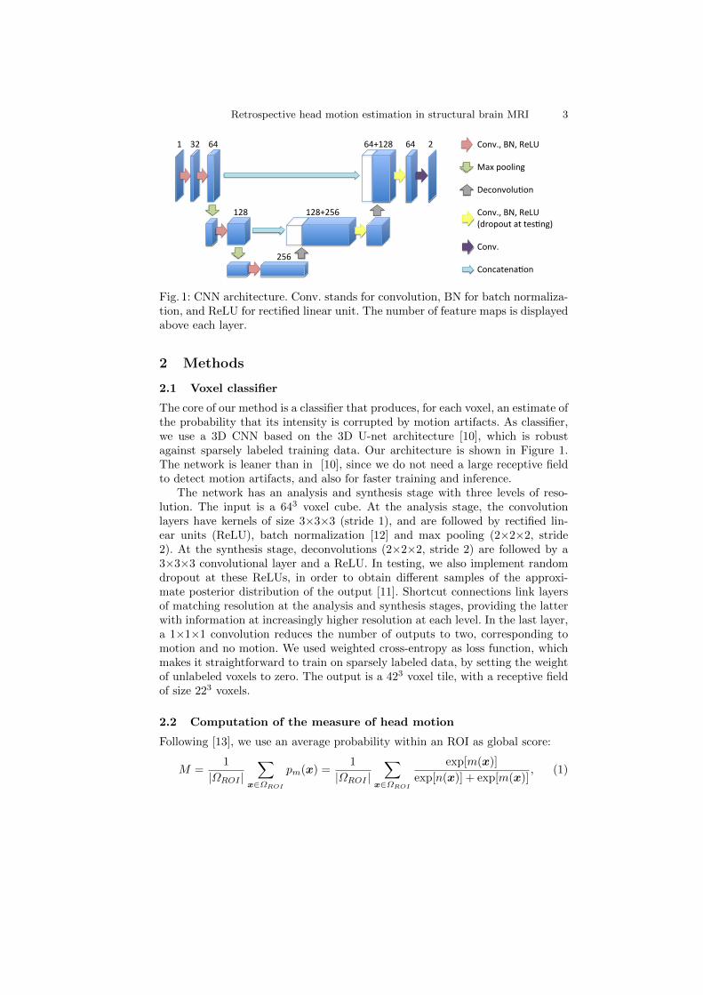
Fig. 1: CNN architecture. Conv. stands for convolution, BN for batch normaliza-tion, and ReLU for rectified linear unit. The number of feature maps is displayedabove each layer.

2 Methods

2.1 Voxel classifier

The core of our method is a classifier that produces, for each voxel, an estimate ofthe probability that its intensity is corrupted by motion artifacts. As classifier,we use a 3D CNN based on the 3D U-net architecture [10], which is robustagainst sparsely labeled training data. Our architecture is shown in Figure 1.The network is leaner than in [10], since we do not need a large receptive fieldto detect motion artifacts, and also for faster training and inference.

The network has an analysis and synthesis stage with three levels of reso-lution. The input is a 643 voxel cube. At the analysis stage, the convolutionlayers have kernels of size 3×3×3 (stride 1), and are followed by rectified lin-ear units (ReLU), batch normalization [12] and max pooling (2×2×2, stride2). At the synthesis stage, deconvolutions (2×2×2, stride 2) are followed by a3×3×3 convolutional layer and a ReLU. In testing, we also implement randomdropout at these ReLUs, in order to obtain different samples of the approxi-mate posterior distribution of the output [11]. Shortcut connections link layersof matching resolution at the analysis and synthesis stages, providing the latterwith information at increasingly higher resolution at each level. In the last layer,a 1×1×1 convolution reduces the number of outputs to two, corresponding tomotion and no motion. We used weighted cross-entropy as loss function, whichmakes it straightforward to train on sparsely labeled data, by setting the weightof unlabeled voxels to zero. The output is a 423 voxel tile, with a receptive fieldof size 223 voxels.

2.2 Computation of the measure of head motion

Following [13], we use an average probability within an ROI as global score:

M =1

|ΩROI |∑

x∈ΩROI

pm(x) =1

|ΩROI |∑

x∈ΩROI

exp[m(x)]

exp[n(x)] + exp[m(x)], (1)


where M is our global motion score, ΩROI is the ROI domain, x is a voxellocation, and pm(x) is the probability that the voxel at location x is motioncorrupted. Such probability is computed as the softmax of n(x) and m(x), whichare the strengths of the activations of the no-motion and motion units at thefinal layer of the CNN, respectively. As much as a single pm(x) is a weak measureof head motion, its average across the ROI provides a robust estimate [13].

3 Experiments and Results

3.1 MRI data and manual annotations

We used two different datasets in this study. The first dataset (henceforth the “in-house” dataset) consists of brain MRI scans from n = 48 healthy children aged7.1-11.5 years, acquired with a 3T Siemens scanner using an MP-RAGE sequenceat 1 mm isotropic resolution. Two separate sets of ground truth annotations werecreated for this dataset: at the scan level (for testing automatic QC) and at thevoxel level (for training the CNN). At the scan level, we made two sets of QCannotations: one by a trained RA (SM), which we used as ground truth (npass =34, nfail = 14), and a second by JEI, with inter-rater variability purposes.

At the voxel level, creating dense segmentations is time consuming and hardto reproduce due to the difficulty of placing accurate boundaries around regionswith motion artifacts, particularly in 3D. Instead, we made sparse annotationsas follows. First, the RA went over the QC-passed scans, and identified slices indifferent orientations (axial / sagittal / coronal, approximately 30 per scan) thatdisplayed no motion artifacts. The voxels inside the brain in these slices were alllabeled as “no motion”, whereas all other voxels in the scan were not used intraining. Then, the RA went over the QC-failed scans, and drew brushstrokes onregions inside the brain that clearly showed motion artifacts, making sure thatthe annotations were highly specific. These voxels were labeled as “motion”,whereas the remaining voxels were not used to train the classifier. The processtook approximately 10-15 minutes per scan.

In order to test our classifier in a practical scenario and assess its generaliza-tion ability, we used a second dataset: the Autism Brain Imaging Data Exchange(ABIDE [14]). Even though effect sizes are notoriously small in autism spectrumdisorder (ASD), ABIDE is a representative example of the type of applicationfor which our method can be useful, since children with ASD might be moreprone to moving in the scanner. We used a subset of ABIDE consisting of then = 111 subjects (68 controls, 47 ASD) younger than 12 years (range: 10− 12).This choice was motivated by: 1. staying in the age range in which children withASD still have increased cortical thickness [15, 16]; and 2. matching the popula-tion with that of the in-house dataset. This subset of ABIDE was acquired onnine different scanners across different sites, mostly with MP-RAGE sequencesat 1 mm resolution (see [14]).

In both datasets, image intensities were coarsely normalized by dividing themby their robust maximum, computed as the 98th percentile of their intensitydistribution. Cortical thickness measures were obtained with FreeSurfer [17].


3.2 Experimental setup

The motion metric from Equation 1 was computed for the scans from bothdatasets as follows. For the in-house dataset, we used cross-validation with justtwo pseudorandom folds (since training the CNN is computationally expensive),ensuring that the number of QC-fails was the same in both. For ABIDE, ratherthan retraining the CCN on the whole in-house dataset, we processed the scanswith the two CNNs that were already trained and averaged their outputs.

The 3D CNNs were trained end-to-end from scratch using a modified versionof their publicly available implementation, which is based on the Caffe frame-work [18]. Data augmentation included: translations; linear mapping of imageintensities (slope between 0.8 and 1.2); rotations (up to 15 degrees around eachaxis); and elastic deformations based on random shifts of controls point andB-spline interpolation (control points 16 voxels apart, random shifts with stan-dard deviation of 2 voxels). Stochastic gradient descent was used to minimizethe weighted cross-entropy. We used different (constant) weights for the positiveand negative samples to balance their contributions to the loss function. Wetrained until the cross-entropy flattened for the training data (i.e., no validationset), which happened at 60,000 iterations (approximately 10 hours on a NvidiaTitan X GPU). In testing, we used a 50% overlap of the input tiles to mitigateboundary artifacts. Further smoothness was achieved by the dropout at testingscheme [11] (probability: 0.5), which also increased the richness in the distribu-tion of output probabilities. The final probability of motion for each voxel wascomputed as the average of the available estimates at each spatial location.

We evaluated our proposed approach both directly and indirectly. For directvalidation, we assessed the ability of the motion score to predict the output ofhuman QC of the in-house dataset. For the indirect validation, we examinedthe relationship between our motion score and average cortical thickness, aswell as the ability of the score to enhance group differences when regressed out.To compute the motion score, we used an ROI (ΩROI) comprising the corticalribbon (as estimated by FreeSurfer) and an underlying 3 mm layer of cerebralwhite matter, computed by inwards dilation with a spherical kernel.

3.3 Results

Qualitative results: Figure 2 shows sagittal slices of four sample MRI scanswith increasingly severe artifacts, along with the corresponding outputs from theCNN: (a) is crisp and motion-free, and few voxels produce high probability ofmotion; (b) shows minimal ringing on the superior and frontal regions; (c) showsmoderate motion; and (d) displays severe blurring and ringing due to motion,such that the CNN produces high probabilities around most of the ROI.

Quantitative results on in-house dataset: Figure 3(a) shows the distri-butions of the motion scores for the two QC groups, which are far apart: anon-parametric test (Wilcoxon signed-rank) yields p = 5 × 10−8. Therefore, aclassifier based on thresholding the score can closely mimic human QC, reaching0.916 accuracy and 0.941 area under the receiver operating characteristic (ROC)


(a)(b)

(c)(d)

0.90.70.50.20.1

Fig. 2: Sagittal slices of four cases and corresponding probability maps (maskedby the ROI, outlined in blue). (a) M = 0.12 (lowest in dataset). (b) M = 0.19.(c) M = 0.25. (d) M = 0.32 (failed QC).

0.1 0.2 0.3 0.4 0.5Motion score

0

2

4

6

8

10

Pro

ba

bili

ty d

en

sity

Motion scores vs. QC group

QC passedQC failed

(a)

0 0.5 1False positve rate

0

0.2

0.4

0.6

0.8

1

Tru

e p

ositi

ve

ra

te

ROC curve (area: 0.94, acc: 0.92)

(b)

2.4 2.6 2.8 3 3.2Cortical thickness (mm)

0

0.5

1

1.5

2

2.5

3

Pro

ba

bili

ty d

en

sity

Distribution of cortical thickness

UncorrCorr

σ2=0.0108

σ2=0.0191

(c)

Fig. 3: (a) Distribution of motion scores for the two QC groups. (b) ROC forautomatic QC based on score thresholding; the dot marks the operating point:91.6% accuracy. c) Distribution of cortical thickness with and without correction.

curve; see Figure 3(b). This performance is close to the inter-rater variability,which was 0.958. We also found a strong negative correlation between our scoreand mean cortical thickness: ρ = 0.66 (95% C.I. [-0.79,-0.46], p = 3 × 10−7).When correcting for motion, the variance of the cortical thickness decreasedfrom 0.0191 mm2 to 0.0108 mm2, i.e., by 37% (R2

adj = 0.42); see Figure 3(c).

Results on ABIDE dataset: Using a Wilcoxon signed-rank test, we founddifferences in motion scores between the two groups (p = 0.03), a circumstancethat can undermine the conclusion of cortical thickness comparisons. We built ageneral linear model for the left-right averaged mean thickness of each FreeSurfercortical region, with the following covariates: age, gender, group, site of acquisi-tion and, optionally, our motion score. Introducing motion as a covariate in themodel changed the results considerably, as shown by the significance maps inFigure 4, which are overlaid on an inflated, reference surface space (“fsaverage”).


(a)(b)(c)(d)(e)(f)

Fig. 4: Region-wise significance map for differences in cortical thickness betweenASD and control group (left-right averaged). The color map represents − log10 p.(a) Inferior-posterior view, model without motion. (b) Lateral view, model with-out motion. (c) Medial view, model without motion. (d-f) Model with motion.

Figure 4(a,d) shows an inferior-posterior view exposing the occipital lobe andlingual gyrus, areas in which increased cortical thickness has been reported inchildren with ASD [16]. The motion-corrected model increases the effect size inthe occipital lobe (particularly the inferior region) and detects differences in thelingual gyrus that were missed by the model without motion – possibly becausethe effect of motion was very strong in this region (p = 5× 10−7 for its slope).

Figure 4(b,e) shows a lateral view, in which correction by motion revealseffects in the temporal lobe and the insula, which would have been otherwisemissed. The thicknesses of both of these regions showed a strong association withour motion score: p = 5×10−9 and p = 2×10−8, respectively. Finally, the modelwith motion also detected missed differences in the mid-anterior cingulate cortex,as shown in the medial view in Figure 4(c,f) (effect of motion: p = 3× 10−8).

4 Discussion

This work constitutes a relevant first step to retrospectively estimate in-scannermotion from structural MRI scans, without requiring external trackers or rawk-space data. The technique not only enables sites without means for specializedMRI acquisition to consider motion, but also makes it possible to reanalyzelegacy datasets correcting for motion, which can considerably change the results– as we have shown on ABIDE, without even fine-tuning our CNN to this dataset.

Our method is specific to population and MRI contrast. However, once a CNNhas been trained, accurate motion estimates can be automatically obtained withthe method for all subsequent scans within a center, with some generalizationability to other datasets. Training datasets for other MRI contrasts can be cre-ated with limited effort (ca. 10 hours), since training relies on sparely labeleddata. Moreover, manual labeling effort could in principle be saved by fine-tuningour CNN to a new dataset, using only a handful of (sparsely) annotated scans.

Future work will follow three directions: 1. Fine-tuning the CNN to otherdatasets; 2. Testing the method on other morphometric measures and ROIs (e.g.,hippocampal volume); and 3. Extension to motion correction, by training on a(possibly synthetic) set of matched motion-free and motion-corrupted scans.

Acknowledgement: This research was supported by the European ResearchCouncil (Starting Grant 677697, project BUNGEE-TOOLS).


References

1. Van Dijk, K.R., Sabuncu, M.R., Buckner, R.L.: The influence of head motion onintrinsic functional connectivity MRI. Neuroimage 59(1) (2012) 431–438

2. Power, J.D., Barnes, K.A., Snyder, A.Z., Schlaggar, B.L., Petersen, S.E.: Spuriousbut systematic correlations in functional connectivity MRI networks arise fromsubject motion. Neuroimage 59(3) (2012) 2142–2154

3. Yendiki, A., Koldewyn, K., Kakunoori, S., Kanwisher, N., Fischl, B.: Spuriousgroup differences due to head motion in a diffusion MRI study. Neuroimage 88(2014) 79–90

4. Reuter, M., Tisdall, M.D., Qureshi, A., Buckner, R.L., van der Kouwe, A.J., Fischl,B.: Head motion during MRI acquisition reduces gray matter volume and thicknessestimates. Neuroimage 107 (2015) 107–115

5. Maclaren, J., Armstrong, B.S., Barrows, R.T., Danishad, K., Ernst, T., Foster,C.L., Gumus, K., et al.: Measurement and correction of microscopic head motionduring magnetic resonance imaging of the brain. PLOS one 7(11) (2012) e48088

6. White, N., Roddey, C., Shankaranarayanan, A., Han, E., Rettmann, D., Santos,J., Kuperman, J., Dale, A.: PROMO: Real-time prospective motion correction inMRI using image-based tracking. Magnetic Resonance in Medicine 63 (2010) 91

7. Tisdall, D., Hess, A., Reuter, M., Meintjes, E., Fischl, B., van der Kouwe, A.:Volumetric navigators for prospective motion correction and selective reacquisitionin neuroanatomical MRI. Magnetic resonance in medicine 68(2) (2012) 389–399

8. Glover, G.H., Li, T.Q., Ress, D.: Image-based method for retrospective correctionof physiological motion effects in fMRI: RETROICOR. Magnetic resonance inmedicine 44(1) (2000) 162–167

9. Batchelor, P., Atkinson, D., Irarrazaval, P., Hill, D., Hajnal, J., Larkman, D.: Ma-trix description of general motion correction applied to multishot images. Magneticresonance in medicine 54(5) (2005) 1273–1280

10. Cicek, O., Abdulkadir, A., Lienkamp, S.S., Brox, T., Ronneberger, O.: 3D U-net:learning dense volumetric segmentation from sparse annotation. In: Lecture Notesin Computer Science. Volume 9901. (2016) 424–432

11. Gal, Y., Ghahramani, Z.: Dropout as a Bayesian approximation: Representingmodel uncertainty in deep learning. arXiv preprint:1506.02142 (2015)

12. Ioffe, S., Szegedy, C.: Batch normalization: Accelerating deep network training byreducing internal covariate shift. arXiv preprint:1502.03167 (2015)

13. Coupe, P., Eskildsen, S.F., Manjon, J.V., Fonov, V.S., Collins, D.L.: Simultane-ous segmentation and grading of anatomical structures for patient’s classification:application to Alzheimer’s disease. NeuroImage 59(4) (2012) 3736–3747

14. Di Martino, A., Yan, C.G., Li, Q., Denio, E., Castellanos, F.X., Alaerts, K., et al.:The autism brain imaging data exchange: towards a large-scale evaluation of theintrinsic brain architecture in autism. Molecular psychiatry 19(6) (2014) 659–667

15. Wallace, G.L., Dankner, N., Kenworthy, L., Giedd, J.N., Martin, A.: Age-relatedtemporal and parietal cortical thinning in autism spectrum disorders. Brain (2010)3745–3754

16. Zielinski, B.A., Prigge, M.B., Nielsen, J.A., Froehlich, A.L., Abildskov, T.J., An-derson, J.S., Fletcher, P.T., Zygmunt, K.M., et al.: Longitudinal changes in corticalthickness in autism and typical development. Brain 137(6) (2014) 1799–1812

17. Fischl, B.: Freesurfer. Neuroimage 62(2) (2012) 774–78118. Jia, Y., Shelhamer, E., Donahue, J., Karayev, S., Long, J., Girshick, R., Guadar-

rama, S., Darrell, T.: Caffe: Convolutional architecture for fast feature embedding.In: 22nd ACM international conference on Multimedia. (2014) 675–678

Retrospective head motion estimation in structural brain ...

Documents