RETRIEVAL OF HANDWRITTEN HISTORICAL DOCUMENT IMAGES

RETRIEVAL OF HANDWRITTEN HISTORICALDOCUMENT IMAGES

A Dissertation Presented

by

TONI MAXIMILIAN RATH

Submitted to the Graduate School of theUniversity of Massachusetts Amherst in partial fulfillment

of the requirements for the degree of

DOCTOR OF PHILOSOPHY

September 2005

Computer Science

c© Copyright by Toni Maximilian Rath 2005

All Rights Reserved

RETRIEVAL OF HANDWRITTEN HISTORICALDOCUMENT IMAGES

A Dissertation Presented

by

TONI MAXIMILIAN RATH

Approved as to style and content by:

R. Manmatha, Chair

W. Bruce Croft, Member

Allen R. Hanson, Member

Paola Sebastiani, Member

W. Bruce Croft, Department ChairComputer Science

To Mila

Ein Rauch verweht,

Ein Wasser verrinnt,

Eine Zeit vergeht,

Eine neue beginnt.

Joachim Ringelnatz

ACKNOWLEDGMENTS

I would like to thank my advisor R. Manmatha for his guidance, support and for

always having an open door for discussion. With his encouragement and enthusiasm

he has inspired me to tackle difficult problems. It was a pleasure to work in the

friendly atmosphere he created. In addition, I would like to thank my committee

members for their valuable input that helped improve this work.

I am also grateful to my colleagues at the Center for Intelligent Information Re-

trieval, particularly Jiwoon Jeon, Jamie Rothfeder, Shaolei Feng and Natasha Mo-

hanty. Their company and collaboration has provided a very pleasant work envi-

ronment. I will miss our weekly multimedia lunches. My collaboration with Victor

Lavrenko has been particularly fruitful. I would like to thank him for our discussions

about information retrieval problems, for sharing his code and for helping out with

many small problems.

I am truly indebted to Maximo Carreras for his friendship and impeccable knowledge

of probability theory, which he shared with me on many occasions. Many thanks

go to my parents, who have inspired in me the desire to learn and explore. They

have sparked my interest in science and languages. I owe my education to them.

My brother Florian and sister Christine have always been there for me during the

last few years, be it during visits home or through many telephone conversations.

I would like to thank them for that. Special thanks go to my wife’s family. They

have provided me with a home away from home with countless cookouts and family

gatherings. Without them, I would not know about the pleasures of grilled sardines

and home-made wine. I am also lucky to have great friends both in Germany and

the United States. Particularly, I would like to thank Andreas Lohr, Artur Ottlik,

vi

Michael Arens, Stephan Wanke, Alexander Czornik, as well as Ibrahim (Slash) and

Anira Dahlstrom-Hakki. Finally, I would like to thank my wife Maria for her love,

patience and support during these years. I could not have done it without her.

This work was supported in part by the Center for Intelligent Information Re-

trieval and in part by grant #NSF IIS-9909073. Any opinions, findings and con-

clusions or recommendations expressed in this material are the author’s and do not

necessarily reflect those of the sponsors.

vii

ABSTRACT

RETRIEVAL OF HANDWRITTEN HISTORICALDOCUMENT IMAGES

SEPTEMBER 2005

TONI MAXIMILIAN RATH

Diplom, UNIVERSITAT KARLSRUHE (TH), GERMANY

M.Sc., UNIVERSITY OF MASSACHUSETTS AMHERST

Ph.D., UNIVERSITY OF MASSACHUSETTS AMHERST

Directed by: Professor R. Manmatha

Historical library collections across the world hold huge numbers of handwrit-

ten documents. By digitizing these manuscripts, their content can be preserved and

made available to a large community via the Internet or other electronic media. Such

corpora can nowadays be shared relatively easily, but they are often large, unstruc-

tured, and only available in image formats, which makes them difficult to access. In

particular, finding specific locations of interest in a handwritten image collection is

generally very tedious without some sort of index or other access tool.

The current solution for this problem is to manually annotate a historical col-

lection, which is very costly in terms of time and money. In this work we explore

several automatic techniques that allow the retrieval of handwritten document images

with text queries. These are (i) word spotting, an approach that clusters word im-

ages to identify and annotate content-bearing words in a collection, (ii) handwriting

viii

recognition followed by text retrieval, and (iii) cross-modal retrieval models, which

capture the joint occurrence of annotations and word image features in a probabilistic

model. We compare the performance of these approaches empirically on several test

collections.

The main contributions of this work are a detailed examination of retrieval ap-

proaches for historical manuscripts, and the development of the first image retrieval

system for historical manuscripts that allows text queries. This system extends the

field of digital libraries beyond machine printed text into historical handwritten doc-

uments. Building such a system involves challenges on numerous levels: the noisy

historical manuscript domain requires adequate image filtering, normalization and

representation techniques, as well as a robust and scalable retrieval framework. We

describe the construction of a prototype system, which demonstrates the feasibility

of the proposed techniques for a large collection of handwritten historical documents.

ix

TABLE OF CONTENTS

Page

ACKNOWLEDGMENTS . . . . . . . . . . . . . . . . . . . . . . . . . . . . . . . . . . . . . . . . . . . . . vi

ABSTRACT . . . . . . . . . . . . . . . . . . . . . . . . . . . . . . . . . . . . . . . . . . . . . . . . . . . . . . . . .viii

LIST OF TABLES . . . . . . . . . . . . . . . . . . . . . . . . . . . . . . . . . . . . . . . . . . . . . . . . . . .xiv

LIST OF FIGURES . . . . . . . . . . . . . . . . . . . . . . . . . . . . . . . . . . . . . . . . . . . . . . . . . .xvi

CHAPTER

1. INTRODUCTION . . . . . . . . . . . . . . . . . . . . . . . . . . . . . . . . . . . . . . . . . . . . . . . . . 1

1.1 Motivation . . . . . . . . . . . . . . . . . . . . . . . . . . . . . . . . . . . . . . . . . . . . . . . . . . . . . . . 31.2 Terminology . . . . . . . . . . . . . . . . . . . . . . . . . . . . . . . . . . . . . . . . . . . . . . . . . . . . . 71.3 Related Work . . . . . . . . . . . . . . . . . . . . . . . . . . . . . . . . . . . . . . . . . . . . . . . . . . . 11

1.3.1 Handwriting Recognition . . . . . . . . . . . . . . . . . . . . . . . . . . . . . . . . . . . 11

1.3.1.1 Image Processing and Features . . . . . . . . . . . . . . . . . . . . . . 141.3.1.2 Page Segmentation . . . . . . . . . . . . . . . . . . . . . . . . . . . . . . . . 16

1.3.2 Document Retrieval . . . . . . . . . . . . . . . . . . . . . . . . . . . . . . . . . . . . . . . 17

1.3.2.1 Offline Documents . . . . . . . . . . . . . . . . . . . . . . . . . . . . . . . . 171.3.2.2 Online Documents . . . . . . . . . . . . . . . . . . . . . . . . . . . . . . . . 20

1.3.3 Image Annotation and Retrieval . . . . . . . . . . . . . . . . . . . . . . . . . . . . . 21

1.4 System Components . . . . . . . . . . . . . . . . . . . . . . . . . . . . . . . . . . . . . . . . . . . . . 231.5 Document Image Data . . . . . . . . . . . . . . . . . . . . . . . . . . . . . . . . . . . . . . . . . . . 24

1.5.1 Dataset Structure . . . . . . . . . . . . . . . . . . . . . . . . . . . . . . . . . . . . . . . . . 241.5.2 Dataset Creation . . . . . . . . . . . . . . . . . . . . . . . . . . . . . . . . . . . . . . . . . . 25

x

2. NOISE, VARIABILITY AND IMAGE PROCESSING . . . . . . . . . . . . 28

2.1 Noise and Variability . . . . . . . . . . . . . . . . . . . . . . . . . . . . . . . . . . . . . . . . . . . . . 28

2.1.1 Handwriting Variations . . . . . . . . . . . . . . . . . . . . . . . . . . . . . . . . . . . . 292.1.2 Document Appearance Variations . . . . . . . . . . . . . . . . . . . . . . . . . . . 312.1.3 Noise in Historical Documents . . . . . . . . . . . . . . . . . . . . . . . . . . . . . . 32

2.1.3.1 Degradation Due to Age . . . . . . . . . . . . . . . . . . . . . . . . . . . 322.1.3.2 Noise from Digitization Procedure . . . . . . . . . . . . . . . . . . . 34

2.1.4 The George Washington Collection . . . . . . . . . . . . . . . . . . . . . . . . . . 36

2.2 Page Segmentation . . . . . . . . . . . . . . . . . . . . . . . . . . . . . . . . . . . . . . . . . . . . . . 372.3 Word Image Processing . . . . . . . . . . . . . . . . . . . . . . . . . . . . . . . . . . . . . . . . . . . 40

2.3.1 Contrast Enhancement . . . . . . . . . . . . . . . . . . . . . . . . . . . . . . . . . . . . . 402.3.2 Artifact Removal . . . . . . . . . . . . . . . . . . . . . . . . . . . . . . . . . . . . . . . . . . 412.3.3 Deslanting and Deskewing . . . . . . . . . . . . . . . . . . . . . . . . . . . . . . . . . . 422.3.4 Word Size Normalization . . . . . . . . . . . . . . . . . . . . . . . . . . . . . . . . . . . 42

3. IMAGE REPRESENTATION . . . . . . . . . . . . . . . . . . . . . . . . . . . . . . . . . . . . . 44

3.1 Features . . . . . . . . . . . . . . . . . . . . . . . . . . . . . . . . . . . . . . . . . . . . . . . . . . . . . . . . 45

3.1.1 Scalar Features . . . . . . . . . . . . . . . . . . . . . . . . . . . . . . . . . . . . . . . . . . . 463.1.2 Profile Features . . . . . . . . . . . . . . . . . . . . . . . . . . . . . . . . . . . . . . . . . . . 463.1.3 1-Dimensional Profiles . . . . . . . . . . . . . . . . . . . . . . . . . . . . . . . . . . . . . 473.1.4 Multidimensional Profile Features . . . . . . . . . . . . . . . . . . . . . . . . . . . 493.1.5 Feature Performance . . . . . . . . . . . . . . . . . . . . . . . . . . . . . . . . . . . . . . . 50

3.2 Feature Vector Length Normalization. . . . . . . . . . . . . . . . . . . . . . . . . . . . . . . 51

3.2.1 Fourier Coefficient Representation . . . . . . . . . . . . . . . . . . . . . . . . . . . 523.2.2 Length of DFT Representation . . . . . . . . . . . . . . . . . . . . . . . . . . . . . . 53

3.3 Word Image Description Language . . . . . . . . . . . . . . . . . . . . . . . . . . . . . . . . . 56

4. WORD SPOTTING . . . . . . . . . . . . . . . . . . . . . . . . . . . . . . . . . . . . . . . . . . . . . . 58

4.1 The Idea . . . . . . . . . . . . . . . . . . . . . . . . . . . . . . . . . . . . . . . . . . . . . . . . . . . . . . . 584.2 Word Image Matching . . . . . . . . . . . . . . . . . . . . . . . . . . . . . . . . . . . . . . . . . . . . 60

4.2.1 Dynamic Time Warping . . . . . . . . . . . . . . . . . . . . . . . . . . . . . . . . . . . . 614.2.2 Matching Word Images with DTW . . . . . . . . . . . . . . . . . . . . . . . . . . 654.2.3 Experimental Setup . . . . . . . . . . . . . . . . . . . . . . . . . . . . . . . . . . . . . . . 664.2.4 Experimental Results . . . . . . . . . . . . . . . . . . . . . . . . . . . . . . . . . . . . . . 68

xi

4.3 Performance Considerations . . . . . . . . . . . . . . . . . . . . . . . . . . . . . . . . . . . . . . . 73

4.3.1 Using Lower Bounds to Speed up Similarity Queries . . . . . . . . . . . 73

4.3.1.1 Lower-Bounding for Univariate Dynamic TimeWarping . . . . . . . . . . . . . . . . . . . . . . . . . . . . . . . . . . . . . . 75

4.3.1.2 Lower-Bounding for Multivariate Time Series . . . . . . . . . 784.3.1.3 Piecewise Constant Approximation . . . . . . . . . . . . . . . . . . 804.3.1.4 Experimental Results . . . . . . . . . . . . . . . . . . . . . . . . . . . . . . 82

4.4 Word Image Clustering Experiments . . . . . . . . . . . . . . . . . . . . . . . . . . . . . . . 85

4.4.1 Heaps’ Law . . . . . . . . . . . . . . . . . . . . . . . . . . . . . . . . . . . . . . . . . . . . . . . 864.4.2 Clustering . . . . . . . . . . . . . . . . . . . . . . . . . . . . . . . . . . . . . . . . . . . . . . . . 88

5. RECOGNITION AND RETRIEVAL . . . . . . . . . . . . . . . . . . . . . . . . . . . . . . 96

5.1 Hidden Markov Document Model . . . . . . . . . . . . . . . . . . . . . . . . . . . . . . . . . . 96

5.1.1 Observation Model . . . . . . . . . . . . . . . . . . . . . . . . . . . . . . . . . . . . . . . . 975.1.2 Transition Model . . . . . . . . . . . . . . . . . . . . . . . . . . . . . . . . . . . . . . . . . . 985.1.3 Recognition with Hidden Markov Models . . . . . . . . . . . . . . . . . . . . 1005.1.4 Recognition Experiments . . . . . . . . . . . . . . . . . . . . . . . . . . . . . . . . . . 101

5.1.4.1 Influence of Transition Model . . . . . . . . . . . . . . . . . . . . . . 1025.1.4.2 Recognition of Large Datasets . . . . . . . . . . . . . . . . . . . . . 104

5.2 Retrieval . . . . . . . . . . . . . . . . . . . . . . . . . . . . . . . . . . . . . . . . . . . . . . . . . . . . . . 106

5.2.1 Language Model Retrieval . . . . . . . . . . . . . . . . . . . . . . . . . . . . . . . . . 1065.2.2 Retrieval Experiments . . . . . . . . . . . . . . . . . . . . . . . . . . . . . . . . . . . . 107

6. CROSS-MODAL RETRIEVAL . . . . . . . . . . . . . . . . . . . . . . . . . . . . . . . . . . 112

6.1 Joint Models for Annotation Words and Features . . . . . . . . . . . . . . . . . . . 113

6.1.1 Cross-Lingual Text Retrieval . . . . . . . . . . . . . . . . . . . . . . . . . . . . . . . 1146.1.2 Cross-Modal Model . . . . . . . . . . . . . . . . . . . . . . . . . . . . . . . . . . . . . . . 116

6.2 Cross-Modal Retrieval . . . . . . . . . . . . . . . . . . . . . . . . . . . . . . . . . . . . . . . . . . . 118

6.2.1 Probabilistic Annotation . . . . . . . . . . . . . . . . . . . . . . . . . . . . . . . . . . 1186.2.2 Content Modeling . . . . . . . . . . . . . . . . . . . . . . . . . . . . . . . . . . . . . . . . 121

6.3 Experimental Results . . . . . . . . . . . . . . . . . . . . . . . . . . . . . . . . . . . . . . . . . . . 123

6.3.1 100 Pages of Test Data . . . . . . . . . . . . . . . . . . . . . . . . . . . . . . . . . . . . 123

xii

6.3.2 1100 Pages of Test Data . . . . . . . . . . . . . . . . . . . . . . . . . . . . . . . . . . . 1296.3.3 10k Pages . . . . . . . . . . . . . . . . . . . . . . . . . . . . . . . . . . . . . . . . . . . . . . . 132

6.4 Learning Behavior . . . . . . . . . . . . . . . . . . . . . . . . . . . . . . . . . . . . . . . . . . . . . . 1336.5 Linguistic Post-Processing of Annotation Results . . . . . . . . . . . . . . . . . . . 135

6.5.1 Constraint Model . . . . . . . . . . . . . . . . . . . . . . . . . . . . . . . . . . . . . . . . 1356.5.2 Experimental Results . . . . . . . . . . . . . . . . . . . . . . . . . . . . . . . . . . . . . 138

6.6 Related Cross-Modal Work . . . . . . . . . . . . . . . . . . . . . . . . . . . . . . . . . . . . . . 1406.7 Synthetic Training Data . . . . . . . . . . . . . . . . . . . . . . . . . . . . . . . . . . . . . . . . . 142

6.7.1 TrueType Font . . . . . . . . . . . . . . . . . . . . . . . . . . . . . . . . . . . . . . . . . . . 1436.7.2 Bitmap Font . . . . . . . . . . . . . . . . . . . . . . . . . . . . . . . . . . . . . . . . . . . . . 1456.7.3 Experiments and Results . . . . . . . . . . . . . . . . . . . . . . . . . . . . . . . . . . 147

7. CONCLUSIONS AND FUTURE WORK . . . . . . . . . . . . . . . . . . . . . . . . 152

7.1 Summary . . . . . . . . . . . . . . . . . . . . . . . . . . . . . . . . . . . . . . . . . . . . . . . . . . . . . . 1527.2 Future Work . . . . . . . . . . . . . . . . . . . . . . . . . . . . . . . . . . . . . . . . . . . . . . . . . . . 154

7.2.1 System Improvements . . . . . . . . . . . . . . . . . . . . . . . . . . . . . . . . . . . . . 1547.2.2 Making the System Practicable . . . . . . . . . . . . . . . . . . . . . . . . . . . . 155

APPENDICES

A. RETRIEVAL INTERFACE . . . . . . . . . . . . . . . . . . . . . . . . . . . . . . . . . . . . . . 159B. DYNAMIC TIME WARPING LOWER-BOUNDING . . . . . . . . . . . . 162

B.1 Fast kNN Sequential Scanning . . . . . . . . . . . . . . . . . . . . . . . . . . . . . . . . . . . . 162B.2 Proof of the Lower-Bound Property . . . . . . . . . . . . . . . . . . . . . . . . . . . . . . . 162

BIBLIOGRAPHY . . . . . . . . . . . . . . . . . . . . . . . . . . . . . . . . . . . . . . . . . . . . . . . . . . 166

xiii

LIST OF TABLES

Table Page

3.1 Feature performance . . . . . . . . . . . . . . . . . . . . . . . . . . . . . . . . . . . . . . . . . . . . . 50

4.1 DTW pseudo code . . . . . . . . . . . . . . . . . . . . . . . . . . . . . . . . . . . . . . . . . . . . . . . 64

4.2 Pruning statistics . . . . . . . . . . . . . . . . . . . . . . . . . . . . . . . . . . . . . . . . . . . . . . . . 68

4.3 Retrieval-by-example performance . . . . . . . . . . . . . . . . . . . . . . . . . . . . . . . . . 70

4.4 Retrieval-by-example (alternate evaluation) . . . . . . . . . . . . . . . . . . . . . . . . . 71

4.5 Matching time . . . . . . . . . . . . . . . . . . . . . . . . . . . . . . . . . . . . . . . . . . . . . . . . . . 72

4.6 Fast sequential scanning algorithm . . . . . . . . . . . . . . . . . . . . . . . . . . . . . . . . . 74

4.7 Lower-bounding results . . . . . . . . . . . . . . . . . . . . . . . . . . . . . . . . . . . . . . . . . . . 84

4.8 Vocabulary size prediction with Heaps’ law. . . . . . . . . . . . . . . . . . . . . . . . . . 87

4.9 Clustering performance . . . . . . . . . . . . . . . . . . . . . . . . . . . . . . . . . . . . . . . . . . . 91

4.10 Clustering performance on a reduced cluster set . . . . . . . . . . . . . . . . . . . . . 93

4.11 Comparison of automatic and ideal Luhn clusters . . . . . . . . . . . . . . . . . . . . 93

5.1 Handwriting recognition results . . . . . . . . . . . . . . . . . . . . . . . . . . . . . . . . . . . 103

5.2 Handwriting recognition results . . . . . . . . . . . . . . . . . . . . . . . . . . . . . . . . . . . 105

5.3 Number of relevant items per query group . . . . . . . . . . . . . . . . . . . . . . . . . 107

5.4 Handwriting retrieval results . . . . . . . . . . . . . . . . . . . . . . . . . . . . . . . . . . . . . 108

5.5 Alternate handwriting retrieval results . . . . . . . . . . . . . . . . . . . . . . . . . . . . . 109

5.6 Handwriting retrieval precision results . . . . . . . . . . . . . . . . . . . . . . . . . . . . . 111

xiv

6.1 Retrieval results using 20 pages of training . . . . . . . . . . . . . . . . . . . . . . . . . 125

6.2 Retrieval results using 20 pages of training (alternate evaluation) . . . . . 125

6.3 Retrieval results using 100 pages of training . . . . . . . . . . . . . . . . . . . . . . . . 126

6.4 Retrieval results using 100 pages of training (alternateevaluation) . . . . . . . . . . . . . . . . . . . . . . . . . . . . . . . . . . . . . . . . . . . . . . . . . 126

6.5 Precision at 5 items using 20 pages of training . . . . . . . . . . . . . . . . . . . . . . 128

6.6 Precision at 5 items using 100 pages of training . . . . . . . . . . . . . . . . . . . . . 128

6.7 Retrieval results on 1100 test pages . . . . . . . . . . . . . . . . . . . . . . . . . . . . . . . 131

6.8 Post-processing annotation evaluation . . . . . . . . . . . . . . . . . . . . . . . . . . . . . 139

6.9 Retrieval performance with post-processing . . . . . . . . . . . . . . . . . . . . . . . . 140

6.10 Queries used in synthetic data experiments . . . . . . . . . . . . . . . . . . . . . . . . . 147

B.1 Fast k-nearest-neighbors algorithm . . . . . . . . . . . . . . . . . . . . . . . . . . . . . . . . 163

xv

LIST OF FIGURES

Figure Page

1.1 Example document image . . . . . . . . . . . . . . . . . . . . . . . . . . . . . . . . . . . . . . . . . . 4

1.2 Another example document image . . . . . . . . . . . . . . . . . . . . . . . . . . . . . . . . . . 5

1.3 Prototype system components . . . . . . . . . . . . . . . . . . . . . . . . . . . . . . . . . . . . . 23

1.4 Segmentation with rectangular stencil . . . . . . . . . . . . . . . . . . . . . . . . . . . . . . 25

2.1 Examples of writing variations . . . . . . . . . . . . . . . . . . . . . . . . . . . . . . . . . . . . 29

2.2 Slant and skew angle . . . . . . . . . . . . . . . . . . . . . . . . . . . . . . . . . . . . . . . . . . . . . 30

2.3 Three word zones and two baselines . . . . . . . . . . . . . . . . . . . . . . . . . . . . . . . . 30

2.4 Historical document artifacts . . . . . . . . . . . . . . . . . . . . . . . . . . . . . . . . . . . . . . 33

2.5 Compression artifacts. . . . . . . . . . . . . . . . . . . . . . . . . . . . . . . . . . . . . . . . . . . . . 36

2.6 Sample page segmentation output . . . . . . . . . . . . . . . . . . . . . . . . . . . . . . . . . . 37

2.7 Scale-space technique illustration . . . . . . . . . . . . . . . . . . . . . . . . . . . . . . . . . . 39

2.8 Contrast enhancement . . . . . . . . . . . . . . . . . . . . . . . . . . . . . . . . . . . . . . . . . . . 40

2.9 Artifact removal . . . . . . . . . . . . . . . . . . . . . . . . . . . . . . . . . . . . . . . . . . . . . . . . . 41

2.10 Deskewing and deslanting . . . . . . . . . . . . . . . . . . . . . . . . . . . . . . . . . . . . . . . . . 42

2.11 Word size normalization . . . . . . . . . . . . . . . . . . . . . . . . . . . . . . . . . . . . . . . . . . 43

3.1 Profile feature examples . . . . . . . . . . . . . . . . . . . . . . . . . . . . . . . . . . . . . . . . . . 47

3.2 Multidimensional profile examples . . . . . . . . . . . . . . . . . . . . . . . . . . . . . . . . . 49

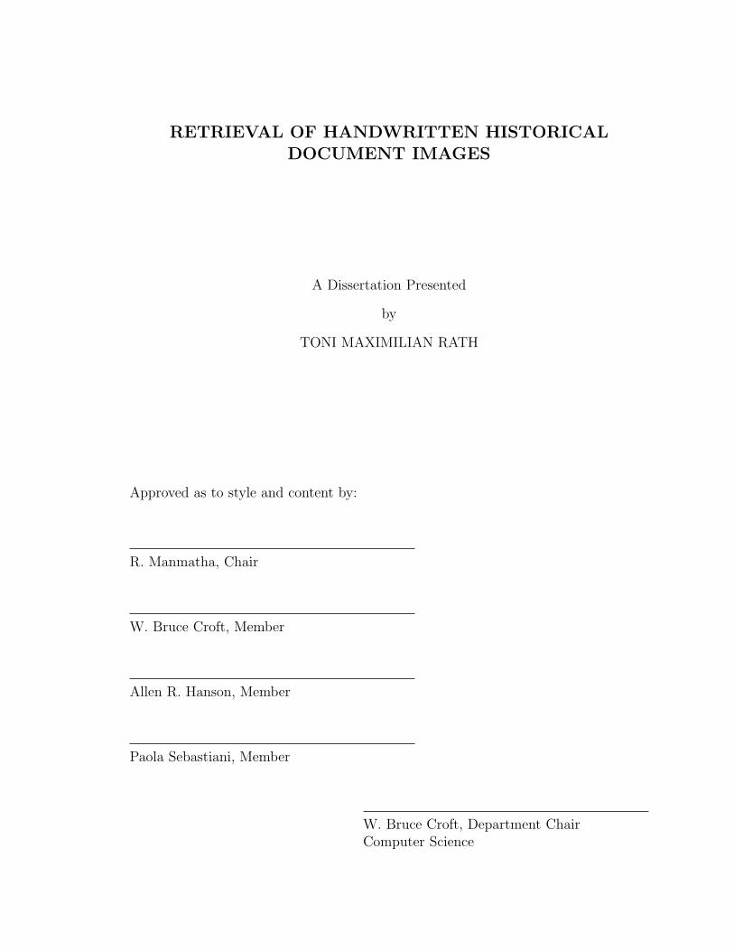
3.3 Approximate projection profile reconstruction . . . . . . . . . . . . . . . . . . . . . . . 53

xvi

3.4 Word error rate versus number of DFT coefficients . . . . . . . . . . . . . . . . . . . 55

3.5 Feature token generation . . . . . . . . . . . . . . . . . . . . . . . . . . . . . . . . . . . . . . . . . 57

4.1 Word spotting process . . . . . . . . . . . . . . . . . . . . . . . . . . . . . . . . . . . . . . . . . . . . 59

4.2 Zipf’s law . . . . . . . . . . . . . . . . . . . . . . . . . . . . . . . . . . . . . . . . . . . . . . . . . . . . . . 60

4.3 Profile alignment . . . . . . . . . . . . . . . . . . . . . . . . . . . . . . . . . . . . . . . . . . . . . . . . 61

4.4 DTW matrix with warping path . . . . . . . . . . . . . . . . . . . . . . . . . . . . . . . . . . . 62

4.5 Dynamic Time Warping constraints . . . . . . . . . . . . . . . . . . . . . . . . . . . . . . . . 64

4.6 Document samples . . . . . . . . . . . . . . . . . . . . . . . . . . . . . . . . . . . . . . . . . . . . . . . 67

4.7 Time series envelope . . . . . . . . . . . . . . . . . . . . . . . . . . . . . . . . . . . . . . . . . . . . . 76

4.8 Lower bound calculation . . . . . . . . . . . . . . . . . . . . . . . . . . . . . . . . . . . . . . . . . . 77

4.9 Multivariate lower bound calculation . . . . . . . . . . . . . . . . . . . . . . . . . . . . . . . 79

4.10 Piecewise constant approximation . . . . . . . . . . . . . . . . . . . . . . . . . . . . . . . . . . 80

4.11 Histogram of tightness values . . . . . . . . . . . . . . . . . . . . . . . . . . . . . . . . . . . . . . 83

4.12 Heaps’ law . . . . . . . . . . . . . . . . . . . . . . . . . . . . . . . . . . . . . . . . . . . . . . . . . . . . . . 87

4.13 Cluster size histograms . . . . . . . . . . . . . . . . . . . . . . . . . . . . . . . . . . . . . . . . . . . 92

5.1 Hidden Markov document model . . . . . . . . . . . . . . . . . . . . . . . . . . . . . . . . . . . 97

6.1 Cross-lingual relevance model . . . . . . . . . . . . . . . . . . . . . . . . . . . . . . . . . . . . 115

6.2 Cross-modal relevance model . . . . . . . . . . . . . . . . . . . . . . . . . . . . . . . . . . . . . 116

6.3 Annotation examples . . . . . . . . . . . . . . . . . . . . . . . . . . . . . . . . . . . . . . . . . . . . 121

6.4 Challenging images . . . . . . . . . . . . . . . . . . . . . . . . . . . . . . . . . . . . . . . . . . . . . 131

6.5 Learning behavior illustrations . . . . . . . . . . . . . . . . . . . . . . . . . . . . . . . . . . . 134

6.6 Hidden Markov Model . . . . . . . . . . . . . . . . . . . . . . . . . . . . . . . . . . . . . . . . . . 136

6.7 TrueType font samples . . . . . . . . . . . . . . . . . . . . . . . . . . . . . . . . . . . . . . . . . . 144

xvii

6.8 Degraded TrueType font samples . . . . . . . . . . . . . . . . . . . . . . . . . . . . . . . . . 144

6.9 Copperplate bitmap font . . . . . . . . . . . . . . . . . . . . . . . . . . . . . . . . . . . . . . . . 146

6.10 Bitmap font samples . . . . . . . . . . . . . . . . . . . . . . . . . . . . . . . . . . . . . . . . . . . . 146

6.11 Retrieval performance using synthetic data . . . . . . . . . . . . . . . . . . . . . . . . . 149

6.12 Synthetic feature distance evaluation . . . . . . . . . . . . . . . . . . . . . . . . . . . . . . 150

A.1 Retrieval user interface . . . . . . . . . . . . . . . . . . . . . . . . . . . . . . . . . . . . . . . . . . 160

xviii

CHAPTER 1

INTRODUCTION

Handwritten document retrieval holds great promise for providing access to his-

torical manuscripts for a large audience. Given a user query, handwritten document

retrieval would find images of manuscripts that are relevant (“answers”) to the query,

which saves the user the tedious work of browsing or reading through an entire col-

lection when looking for a particular document. This work provides a thorough ex-

amination of several retrieval techniques for handwritten historical document images

that allow queries to be entered as text. We also address image processing and feature

representation techniques for degraded document images. The described approaches

have been used in the creation of the first retrieval system for handwritten historical

documents. It is particularly appealing that the queries are textual, a fact that makes

this system very practical. Previous work assumes that users would provide examples

of writing samples that they would like to retrieve, which severely complicates the

formulation of queries.

The first part of this work is concerned with the description of image processing

techniques that are necessary to extract information from handwritten historical doc-

uments. In particular, noise removal, word segmentation, word normalization and

feature extraction will be described.

In the second part, different approaches to annotating (labeling) and retrieving

handwritten historical documents are outlined. These are word spotting, recognition

and retrieval and cross-modal retrieval models. Word spotting is a technique that

builds clusters of unlabeled word images by performing pairwise comparisons between

1

them. Ideally, all word images with the same annotation/transcription are placed into

one cluster. We show how clusters which make good indexing terms can be selected

automatically. Such clusters may then be manually annotated, allowing us to build

a partial index for a document collection, similar to the index in the back of a book.

Previous work has focused on the development of pairwise similarity measures for

word images. Here we extend this work by completing the word spotting process. We

show how to use the similarity measures for word image clustering, and how to select

clusters which make good candidates for indexing.

The recognition and retrieval approach follows the main line of research on an-

alyzing handwritten documents. A recognizer is used to automatically create tran-

scriptions of all manuscripts in a collection. Then standard information retrieval

techniques may be used on the resulting electronic text, in order to find items that

are relevant to a given query. The handwriting recognizer that is used in this work

recognizes words holistically, i.e. without word segmentation, using a Hidden Markov

Model (HMM). We evaluate the error rate of the recognizer on historical manuscripts

and compare the retrieval performance with that of other models.

Cross-modal retrieval models capture the joint distribution of word image features

and annotation terms, building on past work in cross-language information retrieval of

text. This model may be used to either obtain content models from queries or to create

probabilistic annotations which are used in retrieval. The content models are feature

distributions, which may be used to retrieve matching image content. Probabilistic

annotation distributions may be used to estimate term occurrence frequencies in

documents from observed image features. This makes it possible to employ the widely

used language modeling approach to document retrieval. We evaluate our cross-

modal retrieval models, compare their performance with the recognition-and-retrieval

approach and demonstrate their scalability on large datasets.

2

A prototype retrieval system has been built using the cross-modal retrieval model.

Its components and a brief discussion of the user interface are documented in the ap-

pendix. We conclude this work with an outlook on future work and make recommen-

dations on how the current demonstration system can mature into a commercial-grade

product.

1.1 Motivation

Libraries contain extensive collections of handwritten historical documents. Typ-

ically, only a small group of people are allowed access to such collections, because the

preservation of the material is of great concern. In recent years, libraries have begun

to digitize historical document corpora that are of interest to a wide range of people,

with the goal of preserving the content and making the documents available via elec-

tronic media. Examples of such collections are the letters of George Washington at

the Library of Congress (see Figures 1.1 and 1.2 for examples) and Isaac Newton’s

manuscripts at the University of Cambridge.

Historical collections are of interest to a number of people, not just historians, stu-

dents and scholars who need to study the historical originals. For example, biologists

can use handwritten field notes [33] to compare the current state of an ecosystem

with conditions in the past. Paleoclimatologists are also interested in historical hand-

written notes, such as farmer’s diaries, since they often contain references to weather,

which are indicators of the climate in the past.

Unfortunately, digitization alone is not enough to render historical document col-

lections useful for such purposes. Having the information available in an electronic

image format makes it possible to share it with many people across large distances

via the Internet, Digital Versatile Discs (DVDs) or other digital media. However,

the size of a collection is often substantial and the content is generally unstructured,

which makes it hard to quickly find particular documents of interest.

3

Figure 1.1. A scanned document from the George Washington collection.

4

Figure 1.2. Another scanned document from the George Washington collection ina different writing style.

5

Various solutions for this problem that rely entirely on human labor are possible:

a simple way of structuring a collection of historical documents is by ordering them

chronologically. Electronic annotations of volumes or individual pages with the main

subjects of discourse provide access at even finer granularity. A very high level of

detail in content annotation may be achieved with transcription. It allows full-text

search using a traditional text search engine. Because the cost for the electronic

annotation of content increases substantially with the desired level of detail and the

size of the annotated collection, usually a trade-off between detail and cost is chosen.

In the case of the George Washington manuscripts, the Library of Congress decided

to organize the approximately 152,000 page images in 9 series, each with a particular

topic and ordered chronologically. Selected documents were transcribed to allow full-

text search over portions of the corpus [110].

Automatic approaches to content annotation and retrieval are clearly desirable in

order to reduce the often enormous cost of human transcription. Automatic recog-

nition of handwritten historical documents may seem like an obvious choice, but

handwriting recognition has only reached high levels of accuracy in two domains:

these are online recognition, where a writer’s pen strokes are recorded in real-time,

and offline applications with small or highly constrained vocabularies, such as check

processing or automatic mail sorting. Historical documents provide a host of chal-

lenges, including large vocabularies, inconsistent spelling, noisy document images.

Such factors make it difficult to achieve good recognition results, and they require

extra attention during the automatic processing of document images.

This work describes the techniques we have developed for the first automatic

handwritten historical document retrieval system. We examine image processing and

feature extraction techniques, three retrieval approaches and the construction of the

first handwriting retrieval system that uses text queries. This system encompasses all

levels of processing from an unordered collection of digitized images to a user interface

6

for the entire collection. The particular challenges that exist in various processing

stages are addressed with appropriate solutions.

One of the biggest challenges for document image analysis systems is the great

variability of handwriting. Many historical collections are the work of one author,

which limits the amount of variation in the writing. Examples of such collections

include the George Washington collection, Isaac Newton’s handwritten documents

and other collections that were authored by historical personalities. The techniques

presented here assume that the analyzed document collection was produced by a single

writer. This assumption is not strictly necessary. For example, G. Washington, whose

papers are used extensively in this collection, employed multiple secretaries to write

a substantial portion of his documents. Despite the variations in writing style, we

were still able to apply the techniques presented here to his papers.

In the remainder of this chapter, we first define a number of terms which arise

frequently in this work. Then we put our work in context by discussing related work,

followed by a brief overview of the components of our retrieval system for handwritten

documents.

1.2 Terminology

Various terms are used frequently in this dissertation. Some of the most common

ones are defined here to establish a consistent terminology and in order to prevent

confusion with similar related terms. The result may be seen as a mini-glossary, which

the reader can refer to as terms occur.

This work is concerned with handwritten historical documents. In most places, we

replace this somewhat bulky term by just documents or manuscripts1. In places where

1which, taken literally, means written by hand.

7

we discuss other types of documents, we use printed documents or modern documents

to set them apart from handwritten or historical documents.

Our main objective is to look at document retrieval, using a query that is supplied

by the user. The task of retrieval is to rank (order) the documents in the collection

at hand according to their relevance to the query. This ranked list of documents is

then presented to the user in that order, starting with the most relevant document.

Retrieval is not limited to documents, but can often be easily extended to other

retrieval units, such as paragraphs, lines and pages. In cases where this extensibility

is straightforward we do not discuss it explicitly and just speak of retrieval units

or documents, when discussing elements of ranked lists. As the title of this work

indicates, we are retrieving images of text, so the user will always be presented with

an image as the response to a query, be it of a line, a document, or of some other

retrieval unit.

Retrieval systems usually establish an index, which organizes information about

term occurrences in documents in such a way that it facilitates fast retrieval. Indexes

can be as simple as the index in the back of a book, simply listing where certain

important terms occur. Powerful text search engines often store more information,

which may even allow the reconstruction of the original text content of the document

collection the index was obtained from.

The question of what constitutes relevance to a particular query is difficult to

answer and is often subject to debate. For our purposes, we consider a document

relevant if it contains all of the query terms. This simple definition allows us to

objectively assess the quality of various retrieval techniques. It has to be pointed out

however, that most work in information retrieval typically uses a semantic notion of

relevance. For example, in the widely used datasets of the TREC (Text Retrieval)

conference [82], a topic is defined by a set of query words and a document is considered

relevant to the query if it discusses the topic, even if none of the query words are used

8

in the document. This type of relevance definition requires a tremendous amount of

human labor. Queries need to be selected and a large number of documents needs

to be read in order to create relevance judgments. The cost of this approach would

be prohibitive in our case. By using our simple definition of relevance, we are able

to generate queries and relevance judgments automatically and we avoid controversy

about whether a document is relevant or not.

When performing retrieval on documents in inflected languages, we might also

consider documents relevant if they contain all of the query terms in any morphological

variation. In that case, we would consider a document relevant to the query “walked”,

if the document contains the term “walking” because their stem is “walk”. We can

implement this definition of relevance by stemming both the query and the documents,

and then using our earlier definition of relevance. Stemming reduces a morphological

variant of a word to its root. For instance, in English the root form of a word is

obtained by removing plural endings of nouns and using the infinitive in place of

conjugated verbs. Inflections take many different forms depending on the language,

requiring language-dependent stemmers.

Retrieval techniques are generally evaluated by running a set of queries. Intu-

itively, the higher a particular retrieval approach places relevant items in the ranked

list, the better it performs. The two most common measures for judging the qual-

ity of a ranked result list are recall and precision. These measures are defined for

a ranked list of a given length, starting with the highest (potentially most relevant)

rank. Recall is the ratio of the number of relevant documents in the list and the total

number of relevant documents. Precision is the proportion of the relevant documents

in the ranked list. As more and more ranks are taken into account, recall increases

monotonically, because more relevant documents will be found. At the same time

precision typically decreases, because more non-relevant document will be appended

to the list (usually relevant items tend to occur at the top of the ranked list). In

9

the information retrieval literature, it is customary to summarize a retrieval run by

plotting interpolated precision at 11 recall levels (0 up to 1 in steps of 0.1; 0 recall

is defined as the first returned relevant document), which are called recall-precision

graphs. When multiple queries are used, the precision data points are averaged for

the same recall level. Retrieval performance measures may be calculated with the

trec eval program [101], which can also test retrieval results for statistically signif-

icant differences.

In order to summarize a single ranked list with one measure, we will use average

precision, which is the mean of all precision values at ranks where a relevant docu-

ment occurs. When multiple ranked lists (resulting from multiple queries) are to be

evaluated, we use mean average precision, which is the mean of the average precision

values for each of the ranked lists.

This work is concerned with the retrieval of images. We refer to an image of a

manuscript page, of a line of text, and of an individual word with the terms page image

or document image, as well as line image and word image. By page segmentation we

mean the process of breaking down a page into word images. Word segmentation

refers to the segmentation of words into images of the contained characters.

Word images will be considered atomic units in this work, meaning they will not

be broken down further into characters and analyzed in a bottom-up fashion as is

customary in analytical approaches. We advocate a holistic approach to the analysis

of word images. This allows us to avoid the difficult word segmentation problem and

to solve the simpler page segmentation problem. A page segmenter turns page images

into a collection of word images, which corresponds to the representation of electronic

text documents, where the atomic units are also words.

10

1.3 Related Work

Previously published work related to this dissertation falls into the areas of hand-

writing recognition, content-based document retrieval approaches and recent devel-

opments in image annotation and retrieval. In the following sections, an overview of

the relevant work in these fields is given.

1.3.1 Handwriting Recognition

Handwriting analysis research may generally be categorized into one of two ar-

eas [84]: online and offline handwriting. In both fields, Hidden Markov Models

(HMM) are usually the tool of choice for recognition [86]. Originally used in speech

recognition [40], they have later been applied to handwriting, because of the sim-

ilarities to speech.2 HMMs offer a way to infer the value of hidden/unobservable

states (e.g. which words were written) using a sequence of observations (features

extracted from the writing). Two particularly nice properties of HMMs are that

they are computationally tractable using dynamic programming techniques (e.g. the

Viterbi algorithm [25]) and can easily incorporate linguistic knowledge in the form of

word or character bigrams. The latter can substantially improve recognition perfor-

mance. HMMs have been applied at three levels in the recognition process: character

recognition, word recognition and sentence recognition. Some of the most modern

recognizers integrate all three in a hierarchical scheme (see for example [77]). Other

techniques that have been used for handwriting classification include dynamic pro-

gramming techniques and more recently Support Vector Machines (SVM).

In online handwriting recognition, a digital input device is used to record the x and

y coordinates of the pen tip as a function of time and possibly other attributes such as

pressure on the writing instrument, etc. The recognition rates that can be achieved

2The input to both speech and handwriting recognition is sequence data that is used to commu-nicate text.

11

with such rich information are better than 80%, even for very large lexicons [84]. This

success has prompted companies to deploy unconstrained handwriting recognition

functionality in computers, such as TabletPCs and Personal Digital Assistants.

Offline handwriting recognition [84, 107, 115], on the other hand, is the task of

recognition from a digitized image of the writing.3 This branch of research has only

yielded high recognition rates in domains that are highly constrained or have small

vocabularies, such as mail sorting or automatic check processing [115]. Applications

with small vocabularies tend to perform better, because there are fewer alternatives to

select from, resulting in fewer recognition mistakes. If domain constraints are properly

exploited, recognition rates may be improved. For example, a correctly recognized

postal code of an address limits the choices for the city and street names.

Very high recognition rates are often achieved through rejection when the rec-

ognizer confidence is low. For example, the bank check reader described in [27] is

claimed to have a recognition accuracy close to a human reader, but rejects about

30-40% of the checks. Current state-of-the-art offline recognizers achieve recognition

rates of about 60% for vocabulary sizes ranging from 2703 to 7719 words [77] or

55.6% accuracy on a 1600 word lexicon [46]. Recently, recognition rates as high as

91% have been reported for a small single-writer test set of 117 lines [117]. As in most

reported results, the datasets that were used in these experiments were obtained un-

der controlled conditions to ensure straight writing, clean scans and other desirable

properties. This is not the case with historical documents.

As a consequence, the recognition rates that can be expected on handwritten his-

torical documents are lower: Tomai et al. [111] described an approach for mapping a

perfect transcript to the corresponding historical document image, which used recog-

nition. The lexicon of the recognizer was constrained to at most 11 words that were

3The present work is concerned with offline handwriting. Unless we indicate otherwise, ourdiscussion here refers to the offline case.

12

obtained from the perfect transcript, but the alignment accuracy was still only 83%

(some words that had poor image quality were not even considered in the evaluation).

On a larger dataset, Lavrenko et al. [58] demonstrated that recognition of handwrit-

ten historical documents can be done holistically (without character segmentation)

with an accuracy of 55% (65% if out-of-vocabulary words are not considered in the

evaluation). These results were obtained with perfect word segmentation and good

bigram statistics that were estimated using an external corpus.

Handwriting recognition approaches may further be classified into segmentation-

based (or analytical) [77, 84, 107] and holistic analysis methods [64, 65]. Analytical

recognition techniques segment word images into smaller units that can be recognized

in isolation or when grouped. Characters are a natural unit and techniques for recog-

nizing machine printed characters were developed by the optical character recognition

(OCR) community. However, accurately determining the segmentation points cannot

be done without first recognizing the characters. This is known as Sayre’s paradox

(segmentation requires recognition, which relies on segmentation) [103]. It has led

researchers to consider multiple segmentation hypotheses by oversegmenting words

into smaller units, such as strokes and image columns [107, 84]. In these approaches,

the correct segmentation into characters typically arises implicitly from the recogni-

tion process, which attributes segments to recognized characters. Other approaches

use explicit word segmentation. These attempt to segment a word into smaller units

that are believed to be characters, which are then recognized [62].

Holistic word recognition techniques [65, 64, 58] view word images as a unit that

will not be further segmented. They are often motivated by the word superiority ef-

fect, a phenomenon that was first observed by Cattell in 1886 [15] and later confirmed

by Reicher in 1969 [96]. They found that humans have the ability to recognize char-

acters faster than in isolation if they appear in valid (familiar) words. Other evidence

that the global word shape plays an important role in the recognition of words was

13

found by Woodworth [120]. He noted that subjects could read lowercase text faster

than uppercase text, which indicates that the changing word shape in lowercase text

is used by humans when reading. Uppercase letters always have the same size, caus-

ing all-uppercase words to have approximately rectangular shape. In the domain of

handwritten historical documents, other factors make a holistic approach attractive,

such as the high level of noise and the writing variations, which can complicate the

character segmentation.

The survey articles by Vinciarelli [115], Steinherz et al. [107] and Plamondon and

Srihari [84] contain further reading on handwriting recognition.

1.3.1.1 Image Processing and Features

To a great extent, the accuracy of a handwriting recognizer depends on the prepro-

cessing stage and the features which are used to represent the units to be recognized.

Various processing steps need to be performed before the data is fed into a recognizer

[115, 107]. Historical manuscripts often contain a substantial amount of noise that

needs to be addressed, but modern documents also require preprocessing to normalize

writing variations that may adversely affect recognition or retrieval performance.

Often times, scanned pages are slightly rotated (cf. Figure 1.1) or the binding is

not removed from the originals, causing the scans to be warped. Such distortions may

be reversed in the preprocessing stage. Hutchison and Barrett [36] present a technique

for registering a set of documents containing information in a tabular format using the

Fourier-Mellin transform to determine an affine warping transform. Cao et al. [14]

reconstruct orthonormal projection images from pages that were scanned from an

open book.

For historical data sets in particular, the removal of noise, such as border marks,

paper discolorations and similar influences may be desired. Tan et al. [108] reported

a technique for removing the effects of bleed-through (ink that travels through paper

14

from the other side of a page). Manmatha and Rothfeder [70] remove black mar-

gins and long lines that are used as layout elements before they apply their page

segmentation algorithm.

The influence of noise and the lack of contrast in historical manuscripts due to

faded ink may also require careful foreground/background separation. Leedham et

al. compared several separation techniques in [59]. For historical Hebrew manuscripts,

Bar Yosef et al. [123] described a multi-stage thresholding algorithm that works well

for degraded and well-preserved documents.

Pages may contain non-text material, such as figures. In order to separate text

from non-text regions, layout analysis and text detection techniques are necessary.

Antonacopoulos et al. [1] described several algorithms that were submitted to the 2003

ICDAR page segmentation competition for printed documents. Breuel [11] presented

an approach for finding maximal whitespace rectangles, which may be used for layout

analysis. Once regions of text have been determined, they need to be broken down

into lines and words. Relevant work in this area is discussed in more detail in the

following section.

The appearance of word images typically varies in slant (tilt angle of writing) and

skew (rotation angle). Such variations are typically removed, because they complicate

classification tasks. Standard deskewing techniques are described in [10, 118], and

deslanting techniques in [10, 44]. More details are given in chapter 2, where we

describe the image techniques we used in our demonstration system.

The features that are used to represent recognizable image portions also play an

important role. This work builds on features that were described in [89]. Other

work on holistic features is by Madhvanath and Govindaraju [65, 64]. The literature

describing features that are useful for the recognition of writing is large. A good

overview of a variety of features for character recognition may be found in [113].

15

1.3.1.2 Page Segmentation

Page segmentation is an important part of any document analysis process. It

turns a page image into a sequence of word images, which are the atomic units

of our document retrieval system. Since it is one of the first steps in the analysis

of documents, high accuracy is an important consideration. Page segmentation is

usually performed by segmenting a page into lines, and then by further breaking up

lines into words. When complex layout schemes or non-textual elements are used,

e.g. when analyzing images of newspaper pages, a more elaborate process is necessary

to extract blocks of text.

The difficulty of the problem depends largely on the spacing between adjacent

lines or words. Not surprisingly, the segmentation of printed documents (e.g. [47]) is

easier than the segmentation of manuscripts, because of the more consistent spacing.

Mahadevan and Nagabushnam [66] presented a gap metric approach for segment-

ing lines of handwritten text. All connected components are represented by their

convex hull and a minimum spanning tree is used to connect the hulls from centroid

to centroid. Segmenting a line now requires identifying connections between convex

hulls, which are inter-word and not between characters within a word. The authors

proposed a number of techniques to identify thresholds for cutting connections be-

tween convex hulls. Marti and Bunke [74, 76] also employed a gap metrics approach

and proposed another way of picking a segmentation threshold. This algorithm was

evaluated on a modern test collection of 541 text lines and yielded an error rate of

4.5%.

While earlier work has focused on documents of high contrast and neat writing,

recent years have shown an increased interest in historical documents of unconstrained

handwriting, which provide a greater challenge. Feldbach and Tonnies presented an

approach for detecting and separating lines of handwritten text in historical church

registers [23]. Their main problems were bending lines and the tight line spacing,

16

resulting in high overlap of the ascender- and descender-zones of adjacent lines. They

estimated the location of the lower baseline by combining piecewise estimates to it;

the upper baseline is then located in a search region that runs parallel to the lower

baseline. On a collection of 246 lines, this algorithm was able to correctly identify

and segment 90% of the lines.

The present work uses an approach by Manmatha and Srimal [71], which was later

refined by Manmatha and Rothfeder [70]. The technique uses a scale-space approach

[60] to segment word objects, which appear as connected “blobs” when the image is

filtered with an anisotropic Laplacian of Gaussian kernel of a particular bandwidth

(or scale). Manmatha and Rothfeder used a scale selection algorithm to choose the

scale at which word images form connected blobs, but under- and over-segmentations

are avoided.

Finally, we would like to mention that the page segmentation problem has also

been investigated for online handwriting data (see for example [94] for line segmen-

tation and [39] for a simple approach to word segmentation).

1.3.2 Document Retrieval

Document retrieval has been proposed for online handwriting data and offline doc-

uments (both printed and handwritten). Earlier approaches tend to require queries

in the form of writing samples. Then the query can be compared with words in a

collection using a matching function. Some later work supports text querying, which

requires a way of turning textual queries into feature representations or vice versa.

Retrieval may then be performed by matching in feature space or by using textual

representations derived from images in the test collection.

1.3.2.1 Offline Documents

Tan et al. [109] described an approach to retrieving machine printed documents

with a textual query (e.g. in ASCII notation). Their method describes both the query

17

and the words occurring in the document images with features, which may then be

matched in order to identify query term occurrences. This paradigm of working in

the content domain is not just applicable to retrieval, it may also be applied to other

tasks. For example, Chen and Bloomberg [17] described an approach to generating

document summaries from scanned images, which does not use OCR.

Early approaches to retrieving historical manuscript images made use of the word

spotting idea, which was initially developed for speech data [42]. This technique can

locate speech recordings that contain mentions of query words, by comparing a user-

provided template to all candidate locations in a data base. When a 2-dimensional

handwriting signal is transformed into a 1-dimensional signal, similar procedures can

be applied to the handwriting domain.

The word spotting idea for handwritten documents was proposed by Manmatha

et al. [69, 68, 67]. They suggested using a word image matching algorithm to cluster

occurrences of the same word in a collection of handwritten documents. When clusters

that contain interesting index terms are labeled, a partial index can be built for the

document corpus, which can then be used for ASCII querying. Although a word image

matching algorithm with high accuracy was presented and thoroughly evaluated by

Rath and Manmatha [91], the experiments also showed that approaches based on

matching words are computationally expensive and cannot yet be applied to very

large collections. So far, all work on word spotting for document retrieval has focused

on word matching techniques, which only allow retrieval using template queries, based

on word image similarity. In this work, we complete the word spotting process by

grouping word images into clusters, and automatically selecting candidate clusters for

indexing.

Ko lcz et al. [48] described an approach for retrieving handwritten documents

using word image templates. Their word image comparison algorithm is based on

matching the provided templates to segmented manuscript lines from the Archive of

18

the Indies collection. Ko lcz et al.’s experiments only used a small number of queries

and documents, and required multiple manually selected templates of the same word

to yield good results. Since the query templates have to be provided in the image

domain, the approach also does not allow textual queries.

More recently, Srihari et al. [106] have realized the importance of handwritten

document retrieval and presented their own retrieval system that is mostly geared

towards forensics applications such as writer identification. It combines word spotting,

handwriting recognition and information retrieval techniques to allow textual and

image queries for retrieval. The system only allows the retrieval of individual words

or images thereof. Our work is more general, in that it allows the retrieval of units

of text of arbitrary size, including documents, lines and individual words.

Vinciarelli [116] described retrieval experiments with a collection of 200 modern

handwritten documents that were produced by a single author. He compared the

retrieval performance on ground truth transcriptions and automatically recognized

handwriting with a word error rate of 45%. When automatically generated transcrip-

tions are used, the performance is worse with an acceptable decrease in precision.

Edwards et al. [21] described an approach to transcribing and retrieving medieval

Latin manuscripts with generalized Hidden Markov Models. Their hidden states

correspond to characters and the space between them. Only one training instance is

used per character and character n-grams are used, yielding a transcription accuracy

of 75%. The retrieval results seem strong, but the authors performed a non-standard

retrieval evaluation without providing quantitative performance measures. Due to the

choice of dataset, all characters exhibit little variation, so they appear almost as if they

were printed. In terms of difficulty the problem appears to fall somewhere between

isolated handwritten character recognition (often called ICR, Intelligent Character

Recognition) and machine print recognition (i.e. OCR).

19

1.3.2.2 Online Documents

Lopresti and Tomkins [61] described an author-specific technique for searching

online handwriting. They decomposed the query- and target-writing into strokes,

which are then turned into sequences of quantized feature vectors (using feature

clustering). A given query is compared to locations in the database using a dynamic

programming approach, similar to the minimum edit distance algorithm. Recall at

22%/20% precision is 89%/81% for retrieval using roughly 6,000 query words from

two writers.

In [39], Jain and Namboodiri presented an approach to retrieving online handwrit-

ten words from a given template, using dynamic time warping. Words are represented

as one continuous stroke and three features are extracted at each sample point of the

pen trajectory associated with a word. The authors reported a precision of 92%

at 90% recall for individual word image retrieval, which outperforms Lopresti and

Tomkins’ approach above. However, the database is different, making a comparison

difficult.

Kwok et al. [51] described a system for the retrieval of online documents with text

queries. They used a recognizer to create “stacks” (vectors) of alternative recognition

results per handwritten word. These stacks are then compared to a query stack using

traditional retrieval models for document representations in vector space, such as

Okapi [3] and cosine similarity. Their best results yielded about 80% precision at

80% recall.

Russell et al. [99] proposed a system for online handwritten document retrieval,

which uses the concept of “N-best” recognition output (similar to Kwok et al.’s stacks

[51]). A recognizer returns the N best recognition choices per word image, together

with a probability as confidence score. These scores may be used in a probabilistic

document retrieval framework. This and other retrieval techniques showed good per-

formance on a large multi-writer dataset of 3342 documents, when using both textual

20

and template queries. The idea of using multiple words for annotating an image is

also a theme that is common to the work in photograph annotation and retrieval,

which is documented below.

1.3.3 Image Annotation and Retrieval

The cross-modal retrieval system described in this dissertation (chapter 6) is based

on work in the image annotation and retrieval field. Most of the work in this area

has been on general-purpose color photographs (e.g. from the Corel image collection),

showing nature scenes, buildings, people, and other themes. These approaches anno-

tate images with suitable text using recognition. Retrieval may then be performed

using text queries with classical information retrieval models, instead of searching for

matches in the image or feature domain (see e.g. [95]). The general approach is to

model the statistical co-occurrence pattern of image annotations and image features.

All of the approaches described below use annotated training collections to model

the regularities of such patterns. More recently, some approaches have also targeted

video keyframes (e.g. [24, 56]) and 2-D shapes [78].

Mori et al. [79] presented a system that can perform annotations of photographs.

During the training phase, images are divided into regions using a regular grid, and

similar regions are clustered based on color and image intensity gradient features. All

annotation terms of the entire image are inherited by each region and used for learn-

ing an annotation distribution conditional on each cluster via maximum-likelihood

estimation. When a new image is annotated, it is again divided into regions and

an average annotation distribution is created from annotations of the closest region

clusters.

Barnard et al. [6] extended Hofmann’s hierarchical aspect model for text [34] to

the domain of color images with annotations, in order to create a browsable hier-

archy of images and to learn a mapping from image regions to annotation terms.

21

Observed images and their annotations are modeled as being composed of differ-

ent aspects (semantic components) with an enforcement of a hierarchical structure,

which implements the notion of a coarse-to-fine image composition. The Expectation-

Maximization (EM) algorithm is used to train the model, which may then be used

for browsing applications, image retrieval and annotation tasks.

An article by Duygulu et al. [5] showed an entirely new way to view the image

annotation problem. The authors suggested treating object recognition as machine

translation, an approach which they use for annotating general-purpose photographs.

In their framework, images are segmented into regions, which are clustered to produce

an image vocabulary of discrete tokens (“visterms”, each token represents one cluster).

Analogous to learning a lexicon from a parallel corpus in two languages, they train a

translation model which can map image tokens to annotation words.

Jeon et al. [41] used the same representation but viewed the problem as cross-

lingual retrieval and adapted Lavrenko et al.’s cross-lingual relevance model for text

[53]. The resulting cross-media relevance models capture the joint occurrence pattern

of words in two languages (one for annotation words and one for visterms). This

information can then be used for image annotation and retrieval.

Recently, Lavrenko et al. [57] extended the relevance-based approach of Jeon

et al. [41] by removing the need for discrete image representations. The resulting

Continuous-space Relevance Model (CRM) operates on continuous representations of

image regions in terms of multivariate feature vectors, and discrete image annotations

in the form of words. This heterogeneous modeling captures the image representa-

tions in more detail, leading to significantly better performance than the previous

relevance-based models, which operate strictly on discrete data.

Blei and Jordan [8] introduced three generative models for annotated data. The

best-performing model, correspondence LDA, is an extension of Blei et al.’s Latent

Dirichlet Allocation (LDA) [9]. The latter can explain discrete data, such as text, by

22

modeling it as being drawn at random from a mixture of probability distributions.

Each mixture component is seen as a topic, which explains a particular aspect of the

modeled distribution. Correspondence LDA models an image as consisting of multiple

visual aspects, which themselves govern the annotations that are possible for the

entire image. The authors present example results demonstrating good performance

for image and region annotation, as well as text-based image retrieval.

Our cross-modal retrieval model (see chapter 6) builds on the discrete relevance

model retrieval work by Jeon et al. [41] and its extension to continuous-space features

[57].

1.4 System Components

Various processing stages are necessary to transform an unordered collection of

manuscript images into an annotated corpus that supports retrieval with a user in-

terface. Figure 1.3 shows an overview of our prototype system. The principal system

components that this work is concerned with are image processing, feature extraction

and content annotation. We also take a brief look at the retrieval system implementa-

tion with a suitable user interface. The term content annotation is used to refer to the

part of the retrieval system that links manuscript images with text representations

thereof. We have experimented with three approaches: word spotting, document

recognition, and cross-modal models.

Digitalimage

collection

...

Imagesand

annotations. . . . . . . . . .

Indexand

user interface

Imageprocessing

featureextraction

. . . . . . . . . .

Retrieval

systemsetup

Content

annotation...Digitization

Search:

... ...

..

..

.

..

.

..

.. . . .

Captain

Unordered

collectionphysical

...

Featurerepresentation

of collection

Figure 1.3. Main components and processing steps of the currently implementedprototype system.

23

In chapter 2 we describe the various image processing algorithms we use for page

segmentation, noise removal and word image normalization. The features we use

to represent word images are presented in chapter 3. The next three chapters (4

through 6) describe the three approaches for content annotation we have examined:

word spotting in chapter 4, document recognition followed by text retrieval in chapter

5, and cross-media retrieval models in chapter 6. In appendix A we document the

user interface of our prototype retrieval system, which was built using the cross-media

retrieval model.

Before we describe the details of our retrieval system, we briefly explain the struc-

ture of our data and how it was collected in the following section.

1.5 Document Image Data

In this work, we present a number of retrieval approaches for handwritten his-

torical documents. Assessing the relative performance of such techniques solely by

looking at the procedures is very difficult. Convincing evidence of superior perfor-

mance of an approach can only be obtained by testing the retrieval effectiveness on

test data. In the following, we describe the structure and creation procedure of the

datasets we used in our experiments.

1.5.1 Dataset Structure

Images of handwritten words are the atomic units that our retrieval approaches

operate on. Hence, our datasets are sequences of word images, together with a label

for each of the images. The label of a word image consists of the ASCII representation

of all the characters and symbols that are visible in the word image (we ignore parts

of characters from the line above or below the current word image). All word images

result from applying a rectangular stencil (a bounding box) to the document image

that contains them. Handwriting is commonly slanted (tilted) and can be tightly

24

spaced in the vertical direction. As a result, it is often impossible to separate an

entire word image from a page image without also picking up parts from words to the

left and right (or punctuation) and from the line above or below (see Figure 1.4 for

an example).4

Figure 1.4. Unavoidable segmentation of parts from words other than the targetword when using a rectangular stencil (target word inside dashed rectangle).

Each dataset consists of the original page images, the bounding box coordinate

files (one per page image) and a file that assigns ASCII labels to each of the segmented

word images. Organizing a dataset in this fashion is more flexible than just storing

the sequence of word images that is produced by the page segmentation process: the

current approach allows the use of different segmentation files together with the same

page images and ensures that the entire page image is available for processing tech-

niques that need to make use of it. The latter is particularly interesting for techniques

that make use of spatial context when processing word images. The bounding box

coordinates are stored in normalized notation, so they may be applied to page images

at arbitrary resolutions.

1.5.2 Dataset Creation

A significant amount of time has been devoted to the creation of datasets for the

evaluation of retrieval techniques. We used the following process:

4This could be remedied in some cases by preprocessing the page images before the word imagesegmentation. In particular, line deslanting (see section 2.3.3) and line separation would be useful.This is currently under investigation.

25

1. Selection of page images that will form the dataset. Depending on the intended

use for the dataset, various aspects need to be taken into consideration. These

include the quality of the documents (poor training data may impair retrieval

performance), the handwriting style (when used as training data, should be a

reasonable match for the test set), the topic (many words from different topics

make a good training set) and others.

2. Obtain ASCII transcription data for the selected pages. Sometimes transcrip-

tions can be obtained from an online archive (e.g. many transcriptions for the

George Washington collection are available online [110]). If they are not avail-

able, they have to be entered manually by an annotator.

3. Tokenization of the transcriptions. The tokenization process splits transcrip-

tions (which may be organized into lines, pages, . . . ) into a list of terms. Each

entry in the tokenized list corresponds to a word image.

4. Automatic segmentation of page images. This step uses the algorithm proposed

by Manmatha and Rothfeder [70] to turn a collection of page images into a

sequence of word images.

5. Manually correct segmentation output. An annotator manually corrects the

bounding box coordinates using the BoxModify tool [93]. The tool allows the

manipulation of the segmentation output, and the displaying of word image la-

bels (from the tokenization process) overlaid with each word location to quickly

identify and correct alignment mistakes.

The above described procedure is intended for training data and test data with no

segmentation mistakes, which may be used for evaluation under “ideal” conditions.

In a more realistic setting, test data will be automatically segmented (no manual

correction) and there may not be ground truth or it may only be available on a per-

26

page-image basis, not per-word-image. Section 6.3.2 discusses this problem in more

detail.

In chapter 2, we now describe the challenges that historical manuscripts pose and

we discuss how to reduce the influence of noise and handwriting variations with image

processing techniques.

27

CHAPTER 2

NOISE, VARIABILITY AND IMAGE PROCESSING

Before scanned pages of historical manuscripts can be annotated or recognized,

they have to undergo various processing stages. The reason for this is two-fold:

first, the image data may be structured in a way that is unsuitable for downstream

processes. For example, a downstream process might expect individual word images

as input, but the available data is a sequence of page images. Second, the amount

of noise and variability in the input data may complicate further processing. An

example of this are ruler marks on a page which helped the author with the formatting.

Such marks should be removed so that they are not mistaken for parts of words and

misrecognized.

In this chapter, we describe all such processing steps that are performed on the

image data. We begin by describing the noise and variability that is present in

handwritten historical document images. Then we outline the segmentation of input

page images into word images, followed by a description of noise suppression and

image normalization strategies.

2.1 Noise and Variability

When working with historical documents, large amounts of image noise pose a

challenge in addition to the typical writing variations that are present in handwrit-

ten documents. Most work on the analysis of handwritten documents focuses on

modern documents, where the only concern is the variation in the writing (some ex-

ceptions are [23, 111, 21]). The documents used in such work are usually digitized

28

soon after their creation (e.g. see [77]), so that noise due to aging is not an issue. In

this work, we focus on documents that have undergone an aging process, which has

significant implications on their readability. The following sections describe where

noise and variations occur that complicate the recognition or annotation of historical

documents.

2.1.1 Handwriting Variations

Writing is a subconscious and highly individual process. Depending on the person,

their physical condition, writing instrument and other factors, the appearance of the

same text can vary when written at different times. Figure 2.1 shows several examples

of the word the that were taken from the same page, so they were produced within a

short time span. Even in this small sample there is a significant amount of variation

that can be observed. The horizontal t stroke is not always present, varies in length

when present, and sometimes takes on a second role as the stroke that connects the

letters t and h.

(a) (b) (c) (d)

(e) (f) (g) (h)

Figure 2.1. Examples of writing variations during a short period of time. Alloccurrences of the word the were taken from the same page. Notice variations in thehorizontal t stroke, the connection between the t and h, as well as the presence of theopening/hole in the letter e and the size of the t compared to the e.

29

For the purpose of recognizing a word image, handwriting variations are similar

to noise, since they add extraneous information which blurs the underlying structure

that defines a word’s identity. Such variations may have an artistic appeal for a human

reader, but for a recognizer they are distracting details that should be filtered, just

like digitization artifacts and smudges on a page.

skew angle

slant angle

Figure 2.2. Slant and skew angle of a handwritten word.

When looking at the writing of a single person, the most common variations are

differences in slant and skew (see Figure 2.2). The skew of a word is the rotation

angle of the word with respect to the horizontal. Slant is the tilt angle of the writing.

It is common practice in handwriting recognition [107, 115] to normalize the skew

angle to 0 degrees and the slant angle to 90 degrees. Section 2.3.3 describes the slant

and skew normalization techniques that are used in this work.

center zone

descender zone

ascender zoneupper baseline

lower baseline

Figure 2.3. A word image with its three zones and the two baselines.

Another variation that is typical of handwriting is the size of the three word image

zones. Figure 2.3 shows the three zones: the ascender-, center- and descender-zone,

30

which are defined by the upper and lower baselines. The two baselines determine the

location of lower-case characters which have neither ascenders nor descenders (strokes

which reach into the respective zones). The absolute and relative size of the three

zones is often subject to variations. This is problematic if features are used which

measure some location-dependent property in a word image. Feature values (and

therefore positions) need to be comparable across different word images. This can be

guaranteed by resizing the zones so that they occupy predefined fractions of a word

image. Section 2.3.4 describes the word size normalization approach that was used

in this work.

Finally, there are writing mistakes that have been crossed out, as well as variations

and noise which were not intended by the author, such as ink spills and similar prob-

lems. In this work, we do not specifically address such noise. The page segmentation

(section 2.2), however, ignores small ink spots and does not detect them as words.

2.1.2 Document Appearance Variations

Apart from the particular writing style, the author of a document makes various

decisions about the appearance of the document. There are countless ways of arrang-

ing the same text on a page. This does not only affect where and how text is placed,

but also what layout elements are used. For example, non-text elements such as boxes

and rules may be added to the text. Even auxiliary components such as ruler marks

may be mixed in with the actual writing. These are variations that occur as a choice

of the author at the time of the document creation, and as such cannot be avoided.

They require processing techniques that can extract text from documents in semantic

blocks, which are then further analyzed.

Human readers have the ability to break down complex layout schemes into seman-

tically coherent blocks and distinguish textual content from figures, layout elements

or auxiliary components, such as ruler marks. The large amount of handwritten and

31

printed text that is used nowadays has resulted in an essentially unlimited number of

layout schemes. Some documents follow strict rules (e.g. scientific publications), but

quite often little or no layout rules exist (or they are ignored), and where they exist

they may only loosely define the document structure.

This richness in structure explains the large body of work on text detection in

images (e.g. [119, 121, 125]), on determining layout structure (e.g. [11]), and semantic

blocks [30, 1]. The latter category is so challenging that it is even under investigation

for documents that are available in an electronic format, which is used to define the

layout (for example, for the semantic analysis of HTML pages see [80, 13]).

It is clear that a general solution to this problem does not yet exist. Therefore,

in this dissertation we will focus on processing handwriting in documents once it

has been located and separated from other document elements. In section 2.2 some

techniques to discern writing from other objects are touched on.

2.1.3 Noise in Historical Documents

Depending on the age of a document, as well as the quality and timeliness of

preservation efforts, historical manuscripts can exhibit a significant amount of noise.

In addition, capturing an original manuscript as a digital image can also introduce

further noise, depending on how much care is taken in the process. Here we describe

the typical loss of quality that occurs (i) as an effect of time and (ii) during the

digitization process.

2.1.3.1 Degradation Due to Age

Between their time of creation and digitization, historical documents are typi-

cally exposed to environments that adversely affect their quality. Common quality

problems include tearing, water stains, mildew and others. Often times, the value

of a collection is not known for a certain amount of time, so loss of quality occurs

mostly before preservation efforts are made. However, if the preservation is not done

32

correctly, it can actually harm the quality of a collection. For example, the George

Washington collection was initially administered by caretakers who tore signatures

from pages in the belief this did not harm the value of the originals. They also dis-

persed parts of the collection, making it impossible to later collect the entire corpus

in one place [110].

Figure 2.4. Examples of artifacts that typically occur in historical documents. Allimages are taken from the George Washington collection, which is used extensivelyin this work.

Figure 2.4 shows various types of document noise that can be observed throughout

the Washington collection:

1. dirt marks,

2. non-uniform paper color: discoloration due to age,

3. stains and missing parts due to moisture, mildew and tearing,

4. faded ink, often not occurring uniformly across the page,

5. ink bleeding: ink that travels laterally in the paper,

33

6. bleedthrough: ink traveling through the paper from the other side of a page,

Once the damage has occurred to the originals, it is difficult to obtain high qual-

ity images from them. Sometimes scanning under special lighting conditions may

reveal details that seemed lost to the naked eye. However, timely and professional

preservation efforts are the key to high quality document images.

2.1.3.2 Noise from Digitization Procedure

The scanning procedure that is used to capture original documents in an electronic

image format may also have a significant impact on the quality of the resulting images.

Cost is often a major concern, which makes it difficult to use the best available

equipment. Even though using the best possible procedures is desirable, it does not

avoid all sources of noise. The following lists a number of noise sources that are

typical of historical documents:

Digitization from reproductions: Some libraries already have copies of various

documents on microfilm. This serves the dual purpose of making precious orig-

inals available to a greater audience, and to preserve a snapshot of an aging

document collection. Handling original manuscripts is expensive and has to be

performed by trained professionals, so scanning is often done from the micro-

film, which does not require the same level of care and can be automated. This

additional reproduction step adds noise and should therefore be avoided.

Document handling: When the scanning area is larger than the original document,

the background behind the material is scanned. This usually results in borders

of a particular color around a digitized manuscript. Since the originals may

have holes and varying shapes due to disintegrating paper, the borders do not

always have the same appearance.

Ideally, when the manuscripts to be scanned are bound, the binding is removed

and the pages are laid out flat on a scanner. However, when pages of a bound

34

book are scanned, parts of the book may be visible in the digitized result. In

addition, when the page is not flat, it may need to be rectified (see for example

[14]). In the upper right corner of Figure 2.4 a part of a document binding is

visible.

Sensor noise: Scanning sensors are subject to noise. For example, CCD sensor scans

usually contain thermal noise components.

Sensor imperfection: A nonlinear scanner transfer function or hysteresis causes

digitized images to have distorted pixel intensities.

Bilevel scanning: When bilevel scanning is used, the image intensity data is thresh-

olded inside the capturing device. Usually there is no control over the threshold

that is being used. This one-size-fits-all threshold may be appropriate for certain

documents, but others can appear either overexposed or underexposed. While

it may be possible to choose an optimal threshold for printed matter, historical

documents usually should not be scanned in black and white. Grayscale or –

even better – color scanning can help to capture fading ink and may also be

used to distinguish the foreground (ink) from the background (paper, dirt, etc.).

Compression: Space is becoming less of a concern, but some digitization efforts

have relied on lossy image compression formats, such as JPEG, to store scanned

documents. Depending on the type of compression that is used, various artifacts

may be introduced (see Figure 2.5 for an example).

Of course, this list is not complete and the particular types of noise that occur will

always depend on the digitization procedure that is used. Humans are very good at

discerning noise from structure. However, from our discussion here it should be clear

that even if a document appears to be of reasonable quality, it probably contains a

significant amount of noise.

35

(a) Edge image calculated from a lossless TIFF-compressed image.

(b) Edge image calculated from a lossyJPEG-compressed image.

Figure 2.5. Example of compression artifacts. Lossy JPEG compression introducesartifacts that can complicate image processing. The images show the influence of theartifacts on edge detection output.

2.1.4 The George Washington Collection

George Washington, the first president of the United States, was born on February

22, 1732 and died on December 14, 1799. All experiments in the present work were

conducted on a portion of the approximately 152,000 pages of his papers that are

held at the Library of Congress [110]. We will refer to this corpus as the George

Washington collection, even though much of the writing is not Washington’s but

mostly of his secretaries. So the collection has been produced by a small number of

writers, but only one author (George Washington).

All images exhibit quality problems that are typical for historical documents, such

as faded ink, smudges, paper discolorations, ink bleeding and bleed-through. The

images that were made available to us1 were scanned from microfilm reproductions of

the originals, which causes some loss of quality. All images are available in grayscale

with 256 levels of intensity.

Many images have elevated counts of pixels with intensity level 193, an indication

of a sensor imperfection. High-resolution TIFF images stored with lossless compres-

sion are available for most pages, but some are corrupted and only available in a lossy

JPEG format at high compression. That format is inadequate for storing manuscripts,

1We would like to thank the Library of Congress for supplying the scanned manuscript imagesthat were used in this work.

36

because of the artifacts it introduces around sharp edges (for example, strokes). Many

of the manuscripts appear slightly rotated, which makes skew correction necessary.

In the following sections, we describe the processing stages that the manuscript

images undergo, before they are handed to the feature extraction process.

2.2 Page Segmentation

After a collection of historical documents has been scanned, it consists of a series

of page images. Our goal is to perform retrieval on the text contained in the pages,

so we need to detect and extract the contained writing. To do this, each of the

pages is passed to an automatic segmentation process, which produces a series of

rectangle coordinates that can be used to extract word images from the input page.

The detected word images are then passed to the subsequent processing steps in

reading order. Figure 2.6 shows a portion of a page, with overlaid bounding boxes,

as produced by the automatic segmentation process.

Figure 2.6. Portion of a historical document with detected word locations, as pro-duced by the automatic segmentation process.

37

This problem may seem trivial at first glance, but the large amount of extraneous

image content, the variations of ink and paper pixel intensities, and changing line-,

word- and character-spacings make this a challenging problem. As shown above, his-

torical documents often contain various defects and noise, such as border marks, dirt

and faded ink, which can confuse automatic segmentation approaches. Therefore,

simple segmentation techniques such as the gap-metric approach proposed by Marti

and Bunke [76] cannot be applied to historical documents. They assume high-quality

input documents, where the foreground and background can be easily separated and

adjacent lines are spaced far apart. Bunke et al. developed their algorithm for seg-

mentation of modern handwriting data that was carefully prepared to be clean of

noise. Subjects that supplied writing samples were asked to write straight using ruler

marks, to facilitate easy segmentation and processing [74].

In this work, we used the automatic page segmentation approach originally pro-

posed by Manmatha and Srimal [71] and later refined by Manmatha and Rothfeder

[70], which was developed specifically for historical manuscripts. It is based on scale-

space theory [60], which can be used to segment objects of a particular scale in an

image. The notion of scale is implemented by anisotropic Laplacian of Gaussian ker-

nels, which are used to smooth the image in such a way that pixels forming an object

will tend to appear as connected blobs.

Our objects of interest are handwritten words, so the goal is to choose a scale

that allows the segmentation of words, but neither segments individual characters

nor groups words together. Figure 2.7 shows an original image of a phrase and two

scale-space versions of it. The chosen scale in figure 2.7(b) is not suitable for word

segmentation, since blobs in the scale-space image correspond to units smaller than

words (characters and word fragments) in the original. Figure 2.7(c) shows a scale-

space image at the optimal scale for word segmentation. Here, each blob encompasses

all characters in a word, without connecting across words. Manmatha et al.’s tech-

38

(a) Original phrase image.

(b) Non-optimal scale for word segmentation.

(c) Optimal scale for word segmentation.

Figure 2.7. Illustration of a phrase image in scale space at two different scales.

nique works best when the spacing between words and characters is consistent, and

the space between characters is smaller than between words. Our experiments in

section 6.3.1 show that segmentation mistakes have an adverse effect on the retrieval

quality, but the performance decrease when compared to manual segmentation is

acceptable.

Segmentation with this approach typically fails in the presence of layout elements,

extraneous image content (e.g. stamps) and when the spacing is very narrow. In

addition, since the words are segmented using rectangular bounding boxes, the slant of

the words often causes the segmentation of parts from words to the left and right of the

target word. When there is little space between adjacent lines, a word’s bounding box

may also contain parts of words from the line above or below. Section 2.3.2 describes

an approach for removing such artifacts. The page segmentation algorithm removes

borders around pages and some underlining by applying aspect ratio constraints to

detected words. Additionally, detected regions are discarded if they contain very

little intensity variation, which indicates a lack of text content. Therefore, we do not

consider such cases in the further processing of word images.

39

2.3 Word Image Processing

In the current retrieval system, segmented word images undergo various processing

stages that seek to remedy some of the most significant variations and noise that

occur in historical document images. The following is a description of the processing

techniques that we applied to filter noise and to normalize handwriting variations.

2.3.1 Contrast Enhancement

Fading and bleeding ink, as well as discolored paper may cause some word images

to exhibit poor contrast. We enhance the contrast of all word images by scaling the

image intensities linearly to span the maximum range of 0 to 255. This enhances the

contrast of word images with faded ink, while altering images of high contrast only

slightly.

(a) Original image. (b) After contrast enhancement.

Figure 2.8. Example output of the contrast enhancement process.

We have conducted preliminary experiments with more advanced contrast en-

hancement techniques, that seek to fill in faded gaps by enhancing weak “bridges”

of ink. This can be achieved by stronger enhancement of contrast in regions which

have a high likelihood of containing faded ink, such as the area between the two base-

lines. So far, our efforts have not resulted in improved performance, but we believe

that enhancements of weak ink strokes can result in more stable features and better

recognition performance.

40

2.3.2 Artifact Removal

Artifact removal is the process that removes extraneous foreground content which

is not part of the word in the given image. Parts from other words that reach into

the bounding box of the target word image make up the bulk of such problems.

This scenario happens most frequently when the line below or above the current line

contains ascenders or descenders. Figure 2.9(a) shows a typical example of an image

with ascenders from the line below reaching into the bounding box that is returned

by the page segmenter.

(a) Original image with artifacts. (b) Most artifacts removed.

Figure 2.9. Example output of the artifact removal process.

Previously used techniques [43] simply perform binarization of the image and

connected component analysis. Components that do not exceed a certain size are

then removed. While this preserves the main parts of the letters, it also discards

important image components, such as i-dots and parts of the target word that may

have become disconnected due to fading ink. In order to preserve smaller components,

a different algorithm was developed. It fills in the space between the upper and lower

baselines with black, and performs connected component analysis after binarization.

All components that intersect with the upper and lower image boundary are removed.

This is to make sure that only components are removed that reach into the box

surrounding the word image, not components that are entirely contained within the

image. Figure 2.9(b) shows the image in Figure 2.9(a) after artifact removal. It also

reveals one weakness of the current approach: Along with small unconnected parts

of words such as i-dots, dirt is also preserved (next to the letter x). We do believe,

41

however, that i-dots (or, more generally, diacritics in other languages) make very good

features, similar to ascenders and consequently should not be discarded.

2.3.3 Deslanting and Deskewing

Skew and slant, i.e. the rotation and cursive tilt angle of a word are commonly

normalized during the preprocessing stage, since they often have a strong effect on

the feature representations of word images. Skew correction [10, 118] is generally

performed by fitting a line to the local minima of the lower word contour near the

lower baseline, ignoring minima that result from descenders. This is also the approach

we use in this work.

(a) Skewed and slantedword image.

(b) After deskewing. (c) After deslanting.

Figure 2.10. Example outputs of the deskewing and deslanting processes.

Various methods exist for determining the slant angle [10, 44]. One is to deslant

a word at various angles and to use the slant angle that yields the largest distance

between maxima and minima of the upper word contour (or some other measure

of “deslantedness”). Another uses the orientation histogram of the word contour in

order to estimate the slant angle.

In the currently implemented prototype system, both slant and skew are normal-

ized to the same angle (90◦ and 0◦ respectively) before word features are extracted.

Figure 2.10 shows a typical result of the deskewing and deslanting stage.

2.3.4 Word Size Normalization

Some of our features describe locations in a word image, such as the distance of

the first ink pixel from the top of the image. Such features should be comparable

42

across images, even if they are of different sizes. A simple normalization could map

the horizontal and vertical range of the image to the unit interval. However, this

leads to problems with images that do not have descenders or ascenders, such as arm

and Alexandria. With tight bounding boxes around the word images, the bottom of

the word Alexandria corresponds to the location of the lower baseline, whereas the

bottom of the word Regiment would correspond to the bottom of the descender-zone

(because of the descender g). A similar problem occurs when a word does not have

any ascenders.

(a) Input image. (b) After padding to compensate for missingdescender zone.

Figure 2.11. Example output of the word size normalization step.

We normalize the size of words by padding the images at the top and bottom as

necessary to create an empty descender or ascender zone. Then the image parts above

and below the lower baseline are scaled to move the lower baseline to a predefined

location (2/3 of the height from the top).

After the completion of the processing steps described here, the images are passed

to the feature extraction process, which is described in detail in the following chapter.

43

CHAPTER 3

IMAGE REPRESENTATION

Working on images in their original raw format, e.g. a pixel matrix produced by

an upstream processing step, is often inefficient and difficult. Representing images

in terms of features allows (among other things) a more compact and descriptive

characterization of images with limited redundancy. The right feature representation

makes classification easier, so it is an important choice [19, 73]. For example, word

images are often highly redundant because neighboring pixels tend to have similar

pixel intensities. Good feature representations of word images are usually of much

smaller dimensionality, better suited for classification and more easily manageable.

In this chapter, we lay out representation techniques we have chosen for word images

in historical documents.

We advocate a holistic approach to word image analysis, that is, we annotate or

recognize images of entire words, not characters or other units smaller than whole

words. This is reflected by the features we choose for representing word images.

The various classification techniques we employ in this work constrain the features

that can be used. Therefore, we do not present one feature representation that is

used with all classifiers, but rather a variety. All of the representations have in

common that they are derived from scalar features and profile features. Scalar features

measure global image properties such as the image width, and profile features capture

a word’s shape in detail. Based on these features, we describe three word image

representations: (i) raw features (scalars and profiles) that are extracted directly from

44

the images, (ii) feature vectors of constant length with continuous-valued entries, and

(iii) representations that consist of entries from a discrete feature vocabulary.

3.1 Features

Many word images can be distinguished easily by looking at simple holistic fea-

tures such as the width of the word in pixels. However, differing word images with

the same coarse features require a more detailed description, in order to distinguish

between them. Previous work [89, 91] has shown the value of profile-based features

(e.g. projection profiles) for this task. Consequently, the feature set that is used for

representing word images consists of a coarse-to-fine range of features.

Scalar features may be easily compared across different word images (height of one

image vs. height of another), but the profile features we use vary in length based on the

width of a word image and such profiles cannot be compared sample-by-sample, even

when the length of the profiles is normalized.1 A fixed-length description of profile

features may be obtained by computing lower-order coefficients of a DFT (Discrete

Fourier Transform) of each of the original profile-based features. Together, the scalar

and profile-based features then form a vector of fixed length for word images of any

size.

In the following sections, we first describe the scalar and profile features. We then

show how these variable-length representations may be turned into feature vectors

of constant length that may be compared component-by-component. Finally, we

describe the generation of a discrete feature vocabulary that may be used to represent

word images with tokens from the vocabulary. This allows us to represent word images

as “documents” in the “image description language” which is generated by the feature

vocabulary.

1This is, again, due to the variations in handwriting.

45

3.1.1 Scalar Features

Each of the features described here may be expressed using a single number. Some

of them have been used previously (see e.g. [91]) to quickly determine coarse similarity

between word images. The following information is collected from a given image with

a tight bounding box (no extra space around the word):

1. the height h of the image in pixels,

2. the width w of the image,

3. the aspect ratio w/h,

4. the area w · h,

5. an estimate of the number of descenders in the word, and

6. an estimate of the number of ascenders in the word.

While the aspect ratio and area features are redundant, their distributions differ from

those of the height and width features.

3.1.2 Profile Features

These variable-length features capture a word’s shape in much more detail than

single-valued features can. Each feature results from recording a constant number

of values per image column of the word, thus creating a profile or “time series”

(x-axis=time) of the same length as the width of the image.2 We will first look

at 1-dimensional profiles (one extracted value per image column) and then turn to

multidimensional profile features, which record two or more values per image column.

2Treating the feature profiles as time series allows us to apply techniques (e.g. the discrete Fouriertransform) that have been developed for such series.

46

3.1.3 1-Dimensional Profiles

Figure 3.1 shows a set of 1-dimensional profile features and the image (shown

twice in Figures 3.1(a) and 3.1(b) for easy comparison to the feature values) they

were extracted from.

(a) Preprocessed image. (b) With estimated baselines.

(c) Normalized (and inverted) projectionprofile feature.

(d) Partial projection profile (pp) aboveboth baselines (“upper projection pro-file”).

(e) Partial pp between baselines (“mid-dle projection profile”).

(f) Partial pp below baselines (“lowerprojection profile”).

(g) Lower word profile. (h) Upper word profile.

(i) Normalized number of background-to-ink transitions feature.

(j) Normalized variance of column pixelintensities feature.

Figure 3.1. Examples of profile features as extracted from the given preprocessedword images.

47

The profiles are:

Projection profile: Each value in the profile is calculated by summing over the

pixel values in the corresponding image column. Figure 3.1(c) shows the plot of

a typical projection profile. We invert the image before the calculation, causing

concentrations of ink to create peaks, because we would like to measure the

ink contained in each column. The descriptive power of the modified profile

remains unchanged.

Partial projection profile: The three partial profiles in Figures 3.1(d), 3.1(e) and

3.1(f) result from calculating projection profiles for three horizontal strips in

the original image: above, between and below both baselines. A single normal-

ization factor is used for all of the three profiles, because the top and bottom

strips can exhibit low variation of the feature values, when the word has no

ascenders or descenders (e.g. see Figure 3.1(g)). If all profiles were normalized

separately, slight errors in the baseline position estimation could seriously affect

the result.

Upper/lower word profile: Upper (lower) word profile features are computed by

recording – for each image column – the distance from the upper (lower) bound-

ary of the word image to the closest “ink” pixel. Ink pixels are determined by a

thresholding algorithm that classifies pixels into the categories ink and paper. If

an image column does not contain ink, the feature value is computed by linear

interpolation between the two closest defined values. Figures 3.1(g) and 3.1(h)

shows two typical profiles (feature values are inverted).

Background to ink transitions: This feature (see Figure 3.1(i)) records, for every

image column, the number of transitions from the background to an “ink” pixel.

Grayscale variance: The normalized variance of the grayvalue intensities in every

image column is recorded for this feature (see Figure 3.1(j)).

48

The quality of the extracted features strongly depends on good normalization, as

detailed in section 2.3.3. For example, slant can affect the visibility of parts of words

in terms of the word profile features (e.g. the l leaning over the e in Figure 2.2).

3.1.4 Multidimensional Profile Features

The features we present here result from recording two or more feature values per

column of a word image. Taken together, these values form one multidimensional

profile with a length equal to the width of the image they were extracted from.

(a) Preprocessed image. (b) Gaussian-smoothed image, inter-preted as multidimensional profile.

(c) Horizontal partial derivative Gaus-sian kernel response.

(d) Vertical partial derivative Gaussiankernel response.

Figure 3.2. Multidimensional profile features (b)(c)(d) and the preprocessed imagethey were derived from (a). The multidimensional profiles are of dimension 15; featurevalues are visualized as grayscale intensities. The kernels’ scale is σ = 4 pixels.

We investigated the following features:

Gaussian smoothing: The original image is smoothed with an isotropic Gaussian

kernel and resized to a generic height (15). Each line of the resulting image is

now interpreted as a separate feature profile. Figure 3.2(b) shows the feature set

extracted from the original in Figure 3.2(a). All 15 profiles are shown together

with the feature values displayed as grayscale intensities.

Gaussian derivatives: Similar to the feature set obtained from Gaussian-smoothing,

these two sets are obtained from convolving the input image with a horizon-

49

tal/vertical partial derivative of a Gaussian kernel. These filters respond to

horizontal and vertical edges in the original image, which are widely used as

features in computer vision, because they can usually be reliably located. Fig-

ure 3.2 shows the resulting feature sets after convolution with horizontal/vertical

derivative kernels and resizing to the generic height.

3.1.5 Feature Performance

The descriptive power of the above profile features was determined by evaluating

their performance in a whole-word matching experiment [91]. 15 query images were

selected from a dataset of 2381 word images [43] and each of the queries was used to

rank the remaining images in the collection based on their similarity to the query. The

ranking function is based on a Dynamic Time Warping (DTW) similarity measure

defined on profile features (see section 4 for details). Unlikely matches were discarded

beforehand by imposing a threshold on the scalar features that were extracted from

both the query and the candidate image. Discarded images are not included in the

ranked result list.

Test Run Description Mean Avg. Prec.Projection Profile (∗) 50.29%Upper Projection Profile 49.91%Middle Projection Profile 30.83%Lower Projection Profile 24.85%

1-Dimensional ProfilesUpper Word Profile (∗) 64.29%Lower Word Profile (∗) 42.99%Bg./Ink Transitions (∗) 42.46%Graylevel Variance 37.88%Gaussian Smoothing (∗∗) 62.78%

Multidimensional Profiles Gauss. Horizontal Der. (∗∗) 59.63%Gauss. Vertical Der. (∗∗) 52.49%(features marked with ∗) 72.56%

Feature Combinations(features marked with ∗∗) 67.31%

Table 3.1. Performance of various features and feature combinations, measured interms of mean average precision.

50

We ran retrieval experiments using all of the 1-dimensional and multi-dimensional

features separately, followed by combinations of the best-performing profile features

in these two groups. Table 3.1 summarizes the obtained retrieval results using mean

average precision.

Among the one-dimensional profile features, the upper word profile performs best

with 64.29% mean average precision (MAP); among the multi-dimensional profile fea-

tures, the Gaussian-smoothed feature performs best with 62.78% MAP. Since the fea-

tures are designed to respond to different shape characteristics and should complement

one another to some degree, we also analyzed combinations of the 4 best performing

one-dimensional profiles and all three multidimensional profiles. The combination of

the one-dimensional profiles outperforms the multi-dimensional profile combination

with a MAP score of 72.56%.

These results are the motivation for using the combination of upper, lower, and

projection profile together with the background-to-ink transitions profile in further

experiments. However, we are not using the background-to-ink transitions profiles in

the generation of length-normalized feature vectors, which we describe in the next

section. The reason is that these profiles often contain a large number of strongly

localized peaks (high-frequency components), which cannot be adequately captured

by lower order Fourier coefficients (low frequency approximation).

3.2 Feature Vector Length Normalization

While the above profile features capture the shape of a word in great detail, they

vary in length, and cannot be easily compared. One-to-one comparison of samples in

two profiles obtained from different words is usually impossible, simply because the

profiles are of different length. Even if one of the profiles were to be scaled to have

the same number of samples as the other profile, a one-to-one comparison would not

be adequate. The reason for this lies in writing variations, which cause the features to

51

be compressed and stretched in a non-linear fashion. As a consequence, linear scaling

of one of the signals does not cause feature values which correspond intuitively to

appear at the same sample points (see Figure 4.3 for an illustration of this effect).

Chapter 4 describes how two non-linearly scaled signals can be compared using

Dynamic Time Warping. While this algorithm provides a good matching score that

takes into account all details of the compared signals, it can be quite expensive and

its indexability is limited as we will see. With a profile representation in terms of

a vector with constant length, where the components can be compared in a one-to-

one fashion, we could overcome these two shortcomings using fast distance measures

(e.g. Euclidean distance) and spatial access methods [22].

3.2.1 Fourier Coefficient Representation

The Discrete Fourier Transform (DFT) [22] offers a nice way to obtain such a

fixed-length feature vector from profiles of varying length. When the original signal

is described by a number of lower-order DFT coefficients, an approximate recon-

struction is possible. Most of the energy of the original signal is typically contained

in the lower coefficients3, yielding a good approximation of the global feature pro-

file structure (see Figure 3.3), and hence the coarse word shape. Signal noise and

fine-grained writing variations result in higher-order DFT coefficients that are not

useful for classification. Such coefficients are discarded, because they can adversely

affect classification performance. In the next section, we look at how the number of

lower-order DFT coefficients to be used may be chosen empirically.

Figure 3.3 shows clearly that the effect of keeping lower-order coefficients and

discarding the higher-order ones is that of a low-pass filter. Fine-grained detail and

signal noise is ignored by smoothing the profile. The DFT representation also takes

3An exception are signals with many high-frequency components. For an example, see Figure3.1(i).

52

into account that images may have different lengths, since one period of the lowest-

order DFT basis function is equal to the number of sample points in the input signal

(the DFT basis adapts to different input signal lengths).

Figure 3.3. Projection profile time series from Figure 3.1(c), reconstructed using 4lowest-order complex DFT coefficients (4 cosine components, 3 sine components).

The DFT is performed on the time series f = f0, . . . , fn−1 to obtain its frequency-

space representation F = F0, . . . , Fn−1:

Fk =n−1∑l=0

fl · e−2πilk/n, 0 ≤ k ≤ n− 1. (3.1)

Then the first c real (cosine) components and c− 1 imaginary (sine) components are

extracted from the DFT representation for use as scalar features.4 Together with

the 6 scalar features, the first 2 · c − 1 components of F form feature vectors of

constant length (dimensionality) d = 6 + 3 · (2 · c− 1) (we use DFT coefficients from

3 profiles: projection profile, upper, and lower profile). Most of our experiments use

c = 4, that is, a total of 27 features. We normalize the range of feature values along

each dimension to lie in the range [0, 1]. Then all continuous-space feature vectors of

constant length are members of the feature space F = [0, 1]d.

3.2.2 Length of DFT Representation

As we have pointed out in the previous section, the lower-order DFT coefficients

capture the coarse word structure, while higher-order DFT coefficients either result

from noise or writing variations which may have an adverse effect on the quality of

4For real-valued signals, the first imaginary (sine) coefficient of the DFT is always 0.

53

a classification process that uses the coefficients as features. This immediately raises

the question of how many coefficients to use. When the number is chosen too small,

relevant information about the structure of an image is discarded. On the other hand,

using too many coefficients will introduce noise into the feature representation, which

is likely to decrease classification performance.

In order to determine the ideal number of DFT coefficients, we recorded the word

image recognition performance for various lengths of the frequency space represen-

tation. The experiment uses the 20-page dataset and 20-fold cross-validation setup

described in [58]: 19 pages are used as the training set, while the word images in the

remaining page are recognized. Classification is performed using 1-nearest-neighbor

on a feature vector consisting solely of DFT coefficients from three profile features

(projection profile, upper & lower profile; see section 3.1.2).

The coefficients in the frequency-space representation vary in very different ranges.

Lower-order coefficients usually have a much higher magnitude than higher-order

coefficients. We used both the raw coefficients (“No feature normalization”) and a

feature vector where all dimensions have been normalized to lie in the range [0, 1]

(“With feature normalization”). Figure 3.4 shows the Word Error Rate (WER) (1−

classification rate) as a function of the number of DFT coefficients. One coefficient

refers to both the real and imaginary part of a coefficient, so the feature vector for c

coefficients from one profile has 2c−1 components (we discard the first sine coefficient,

because it is always zero).

The first thing to note about the graph is the location of the minimum word

error rate. In the run with feature normalization, the minimum occurs at 6 coef-

ficients (WER=47.9%); in the run without normalization it occurs at 8 coefficients

(WER=53.2%). The run with feature normalization performed better, but also re-

quires a more careful selection of the number of DFT coefficients: the error rate rises

quickly with higher numbers of coefficients, whereas the run with non-normalized

54

0.45

0.5

0.55

0.6

0.65

0.7

0.75

0.8

0.85

0.9

0 10 20 30 40 50 60 70 80 90 100

Wor

d er

ror r

ate

Number of DFT coefficients

With feature normalizationNo feature normalization

Figure 3.4. Word error rate as a function of the number of DFT coefficients. Thetwo runs show the results with and without normalizing each feature vector dimensionto the range [0, 1].

feature vectors remains roughly at the same word error rate even for higher-order

coefficients. The stable performance for a large range of mostly higher-order DFT

coefficients can be attributed to the magnitude of the coefficients. The coefficient

magnitudes decrease rapidly for increasing frequencies, causing higher-order coeffi-

cients to have a negligible impact on the distance we use for the nearest-neighbor

classification.

The normalized run confirms our intuition about the descriptiveness of features:

when too few coefficients are used, relevant information about a word’s structure

is discarded, leading to poor classification performance. When the right number of

coefficients is used, the word error rate is minimal, but rises again for higher numbers,

when noise and writing variations taint the word image representation.

We predict that the ideal number of DFT coefficients to use depends on the quality

of the preprocessing. If the preprocessing is not effective at normalizing writing

variations, the minimum error rate will be reached at a smaller number of coefficients,

because higher-order coefficients will be too noisy to aid in classification of word

55

images. On the other hand, if the preprocessing removes most of the variations, even

higher-order coefficients will contain information that can be used to compare the

structure of a word image at a fine level of detail.

To allow a direct comparison of our performance figures with those in previously

published work, most of our DFT coefficient representations in this work use c = 4

complex components (7 real coefficients) to represent a single profile feature. With

the DFT coefficients from 3 profiles (projection, upper and lower profile) and 6 scalar

features, this yields a total of 27 features. We note that while c = 4 did not yield the

lowest word error rate in our experiment above (cf. Figure 3.4), it is very close to the

optimal setting (c = 6) with a comparable word error rate.

3.3 Word Image Description Language

Two of the retrieval techniques that are described in this work were originally

developed for cross-lingual information retrieval of text documents [53]. The cross-

lingual framework allows a user to formulate a text query in a familiar language

(e.g. English) and retrieve documents in a foreign language (e.g. French). We can

extend this paradigm to images of words, which can be viewed as being the trans-

lation of their ASCII equivalent. In that sense, images of words are an equivalent

representation of an ASCII word in an “image language”. When we represent word

images with (one or more) terms from a discrete image description dictionary, the

cross-lingual retrieval approach can be applied to the domain of handwritten word

images. The retrieval then spans two different media types and will thus be referred

to as cross-modal retrieval.

In previous work [20, 41], continuous-space feature vectors have been turned into

discrete feature tokens using k-means clustering. This spawns a vocabulary consist-

ing of discrete items (henceforth tokens), which can be used to describe originally

continuous-valued feature vectors with a discrete token. We believe that the clus-

56

feature value range ob−served in training data

featurevalue

bin set 2

bin set 1

bin 1 bin 2 bin 10bin 9. . . . . .

bin 1 bin 2 . . .. . . bin 9bin 8

Figure 3.5. Illustration of the binning technique that is used to map continuousfeature values to discrete feature tokens.

tering of entire feature vectors corresponds to a premature classification decision in

feature space that may remove details which could aid in a subsequent classification.

We create a word image description vocabulary that preserves more detail by

using a discretization strategy that proceeds in a dimension-by-dimension fashion.

The observed range of training feature values in each dimension is divided into 10

quantization steps (or bins; see top portion of Figure 3.5) and another 9 steps of the

same width, which overlap by half a bin size (bottom portion of Figure 3.5). Counting

all dimensions of a d-dimensional feature vector, we get 19 · d bins. Each of these

bins is assigned a unique feature token. These 19 · d feature tokens form the discrete

feature vocabulary F .

The reason for using the second set of nine bins is that feature values, which

should be considered similar, might be mapped to different bins and will thus be

assigned different tokens. Using the second set of bins guarantees that two similar

feature values will always be assigned at least one common feature token.

In this chapter, we have described three feature representations for word images:

(i) raw scalar and profile features as they are extracted from the word images, (ii)

length-normalized feature vectors consisting of scalar features and DFT coefficients

that are extracted from profiles, and (iii) feature tokens from a vocabulary of dis-

cretized feature values. In the following three chapters, we discuss approaches for

retrieving handwritten documents, which are based on these representations.

57

CHAPTER 4

WORD SPOTTING

Word spotting is a technique for creating partial indexes for handwritten historical

document collections, similar to indexes in the back of books. It was initially proposed

by Manmatha et al. [69] and has prompted a number of publications that propose

algorithms and features for the approach [71, 88, 91, 89, 98]. Word spotting takes

an unlabeled collection of word images and clusters them using an image matching

algorithm. Ideally, the clustering would create groups of images with the same label.

Then “interesting” clusters may be labeled manually and an index for the clustered

collection may be built, similar to indexes in the back of books. Here we present

the word spotting idea, and the contributions of this work to the realization of the

technique. These are Dynamic Time Warping (DTW) word image matching, which

we compare to a number of other techniques, our extension of Keogh’s DTW indexing

approach for 1-dimensional time series [45] to multidimensional time series and word

image clustering experiments which complete the word spotting process.

4.1 The Idea

The idea of word spotting (see Figure 4.1) is to use image matching for calculating

pairwise “distances” between word images, which can be used to cluster all words oc-

curring in a collection of handwritten documents. Ideally, each cluster would contain

all the words with a particular annotation (without the annotations being known).

Clusters that contain terms which are “interesting” for an index for the document

collection are selected and labeled manually. By assigning the cluster labels to all

58

word images contained in a cluster, we get a partial transcription of the document

collection. This in turn allows us to create a partial index for the collection, which

permits the retrieval of text portions that contain only the manually assigned labels.

Figure 4.1. An illustration of the Word spotting process. Documents are segmented,and distances between word images are calculated. After clustering the word images,some clusters are manually labeled and can be used as index terms.

Early work in information retrieval by Luhn [63] gives some insight into what

makes clusters “interesting”. A plot of term frequencies, where terms are ordered by

decreasing frequency of occurrence, exhibits a distribution that is known as Zipf ’s law

[127].1 That is, the frequency of the k-th most frequent term has a frequency that is

f0/k, where f0 is the frequency of the most frequent term. Luhn argued that index

terms should be taken from the middle of that distribution. Figure 4.2 shows an

example of the actual distribution of term frequencies and the distribution predicted

by Zipf. Note the large amount of mass that is concentrated in high-frequency terms

and the long tail of the distribution to the right, which continues beyond the shown

range. Of course, it would be desirable to index all terms that occur in a collection,

1The use of the word law is deceiving. Zipf’s observation is of an empirical nature, but oftenprovides a reasonable fit to the data.

59

as many modern information retrieval systems do. Luhn’s contribution may be seen

as identifying the best candidates for an index when only a fixed number of terms

can be indexed.

50 100 150 200 2500

200

400

600

800

1000

1200

terms (ordered by frequency)

term

freq

uenc

y

actual distributionZipf’s law

Figure 4.2. Zipf’s law: The plots show the actual distribution of term frequenciesand the prediction made with Zipf’s law based on the actual frequency of the mostfrequent term. The collection size is 21324 words; only the left-hand portion of thegraph is shown.

High-frequency terms (left side of the plot) are often stop words, such as and/the/. . . ,

which have no discriminating power, because they occur in virtually all documents.

Terms with very low frequencies are often sporadic in the sense that their occurrence

is not correlated to the topic of the text they occur in. Such terms are not descriptive

of the content in the collection and may be omitted from the index. Terms that are

descriptive of the content can often be found in the middle of the plot. Their repeated,

but not excessive use suggests that they are essential to describing the content of the

collection and should consequently be part of the index.

In the following sections we assume the output of a page segmentation algorithm

and describe approaches to matching pairs of word images and clustering experiments.

4.2 Word Image Matching

One of the key parts of the word spotting approach is the image matching tech-

nique for comparing word images. Several techniques have been investigated [88, 91,

60

98], with the best performing being Dynamic Time Warping matching [91], which we

explain here in detail.

For DTW matching, word images are represented by multidimensional profile

features (see section 3.1). These profiles are then matched using DTW, a dynamic

programming algorithm that is able to account for writing variations, which cause

the profile features to be compressed and stretched nonlinearly with respect to one

another.

samples

(a) Linear scaling alignment.

samples

(b) Dynamic Time Warping alignment.

Figure 4.3. Two profiles, aligned using linear scaling and Dynamic Time Warping.DTW ensures that only corresponding locations will be compared.

DTW is described in detail in [102]. Its advantage over simple distance mea-

sures, such as linear scaling followed by a Euclidean distance calculation, is that it

determines a common “time axis” (hence the term time warping) for the compared

signals, on which corresponding profile locations appear at the same time. Due to

the variations in handwriting, two profiles of the same word do not generally line up

very well if they are just scaled linearly (see Figure 4.3).

4.2.1 Dynamic Time Warping

Dynamic Time Warping is a dynamic programming algorithm that finds corre-

sponding locations in two signals and calculates a cumulative matching cost from all

correspondences. Figure 4.4 illustrates this process: two signals (word images in this

61

case) are arranged as shown to form the two axes of a matrix. By aligning corre-

sponding samples in the two signals (dashed lines in the figure), a warping path from

the lower left to the upper right of the DTW matrix arises. The cost of matching the

two signals is the cumulative cost of aligning all corresponding sample pairs along the

path. A local distance measure determines the cost of matching two aligned samples.

DTW recovers correspondences between sample locations by finding the warping path

with the minimum accumulated sample alignment cost.

Typically, warping paths are constrained to remain close to the diagonal. This

is called a global path constraint (shaded region in Figure 4.4). By constraining the

warping path to lie within that region, pathological warpings, which map a small

portion of one signal to a large portion in the other, are prevented.

warping path

valid warpingregion (global

path constraint)

Figure 4.4. Dynamic time warping algorithm: two word images are compared byaligning corresponding locations. The result is a warping path through the DTWmatrix.

Formally, when determining the DTW-distance2 dist(X,Y) between two time

series X = (x1, . . . , xM) and Y = (y1, . . . , yN), a matrix D ∈ IRM×N is built, where

2dist(·, ·) does not satisfy all metric axioms.

62

each entry D(i, j) (1 ≤ i ≤ M, 1 ≤ j ≤ N) is the cost of aligning the subsequences

X1:i and Y1:j.

Each entry D(i, j) is calculated recursively from some D(i′, j′) plus an additional

cost d, which is usually some distance (e.g. Euclidean) between the samples xi and

yj. For instance, our implementation of the algorithm uses

D(i, j) = min

D(i, j − 1)

D(i− 1, j)

D(i− 1, j − 1)

+ d(xi, yj). (4.1)

The recursive definition of D(i, j) based on the three given values is a local conti-

nuity constraint. It determines which sample pairs (positions in the matrix) may be

connected to form a warping path. The constraint in equation (4.1), which is also

shown in graphical form in Figure 4.5(a)), ensures that no sample in any of the two

input signals can be left out from the warping path. Other continuity constraints

allow skipping of samples. For a more detailed discussion of continuity constraints

and alternatives to the one used in this work, we refer the reader to [102].

Table 4.1 contains pseudo-code for the DTW algorithm (adapted from [112]) us-

ing the local continuity constraint from Figure 4.5(a). The algorithm determines

a warping path composed of index pairs ((i1, j1), (i2, j2), . . . , (iK , jK)), which aligns

corresponding samples in the input sequences X and Y. Our implementation of

DTW uses the Sakoe-Chiba band [100] global path constraint (see Figure 4.5(b); the

warping path must lie in the shaded region), but the Itakura parallelogram [38] is also

a popular choice. As a side effect, the constraint speeds up the computation of the

DTW matrix, since it does not have to be entirely evaluated. We use r = 15 samples

in our implementation of the word matching algorithm, which was chosen empirically

to optimize matching performance on a small subset of word images. Recent work

63

D(i−1, j−1) D(i, j−1)

D(i, j)

D(i−1, j)

(a) Local continuity constraint,showing valid neighborhood rela-tionships in a warping path.

���������������������������������������������������������������������������������������������������������������������������������������������������������������������������������������������

���������������������������������������������������������������������������������������������������������������������������������������������������������������������������������������������

(1, 1)

(M, N)

r

r

r

r

(b) Global path constraint. The warpingpath must lie in the shaded region aroundthe DTW matrix diagonal.

Figure 4.5. Constraints used in the current dynamic time warping implementation.

[87] shows that the shape of the global path constraint can be adapted, leading to

faster DTW computations and better matching performance.

Input: X = (x1, . . . , xM) and Y = (y1, . . . , yN),distance function d(·, ·)

Output: DTW matrix DAlgorithm:1. D(1, 1) = d(x1, y1);2. for i = 1 : M3. D(i, 1) = D(i− 1, 1) + d(xi, y1);4. for j = 1 : N5. D(1, j) = D(1, j − 1) + d(x1, yj);6. for i = 2 : M7. for j = 2 : N

8. D(i, j) = min

D(i, j − 1)D(i− 1, j)D(i− 1, j − 1)

+ d(xi, yj);

Table 4.1. Pseudo code for the DTW algorithm (without backtracking).

Once all necessary values of D have been calculated, the warping path can be

determined by backtracking the minimum cost path starting from (M, N). However,

we are just interested in the accumulated cost along the warping path, which is stored

64

in D(M, N). As it is, this matching cost is smaller for shorter sequences, so we offset

this bias by dividing the total matching cost by the length K of the warping path,

yielding

dist(X,Y) = D(M, N)/K. (4.2)

4.2.2 Matching Word Images with DTW

We represent word images with single- or multi-dimensional profile features (see

chapter 3). Single-dimensional profiles that were extracted from the same word have

the same length, and may be “stacked” to create multidimensional profiles. Hence,

when matching word images, the sequences X and Y consist of samples of dimen-

sionality d ≥ 1, i.e. xi, yj ∈ IRd. This ensures that all profiles are warped in the same

manner.3

In order to use DTW to match such profiles, we need to define a distance measure

d(·, ·) that determines the (local) distance between two samples in a profile. Our

implementation uses the square of the Euclidean distance

d(xi, yj) =d∑

p=1

(xi,p − yj,p)2, (4.3)

where the index p is used to refer to the p-th dimension of xi and yj. With this

distance measure defined, we can now calculate the matching distance between two

word images by comparing their profile features using DTW and equation (4.2). Then,

our DTW matching algorithm in Table 4.1 computes

dist(X,Y) =1

Kmin

{K∑

k=1

d(xik , yjk)

}=

1

Kmin

{K∑

k=1

d∑p=1

(xik,p − yjk,p)2

},

i.e. the mean alignment cost along the path with the minimum total cost.

3Other work by Ko lcz et al. [48] warped various profiles separately, potentially using differentdistortions, although all profiles were originally determined from the same word image.

65

4.2.3 Experimental Setup

The performance of the DTW word image matching algorithm was evaluated

in a retrieval-by-example setup, where word images in a collection are ranked by

decreasing similarity to a given template. Experiments were conducted on two test

sets of different quality, both 10 pages in size (2381 and 3370 word images). The first

set is of acceptable quality, see Figure 4.6(a)). The second set is very degraded (see

Figure 4.6(b)) - even people have difficulties reading these documents. We used this

data set to test how badly matching algorithms perform on manuscripts of such poor

quality. Each page in the two test sets was segmented into words with an automatic

page segmentation procedure [71]. While the quality of the segmentation algorithm

has been improved in the meantime [70], we used the same segmentation results as

in [43] for comparability.

We conducted four experiments on the test sets and compared the performance of

various matching approaches. Each experiment involves selecting one of the above two

data sets and identifying a subset that will be used for querying. Each of the queries

is used to rank the images in the dataset according to their similarity to the query.

The similarity scores are determined by a matching algorithm. Four experiments were

conducted:

Experiment A: 15 images from test set 1 were selected as queries.

Experiment B: All images in test set 1 were used as queries. This yields a total of

2381 query images, 9 of which do not contain any letters.4

Experiment C: 32 images from test set 2 were selected as queries. 13 of these

images contain words that occur only once in the collection.

4These images are the result of segmentation errors.

66

Experiment D: All images in test set 2 were used as queries. This yields a total of

3370 query images total, 108 of which do not contain any letters.4

Experiments A and C were initially proposed by Kane et al. [43]. We use their

query sets to provide comparable performance figures. Due to the small size of these

sets, they allow us to test algorithms which would otherwise take too long to run

on the entire dataset. Experiments B and D are exhaustive query sets which do not

suffer from potential bias that may have been introduced by the query selection for

experiments A and C.

(a) Acceptable quality (set 1).

(b) Significantly degraded (set 2).

Figure 4.6. Document samples from the Dynamic Time Warping testbeds, showingthe differing quality.

In order to reduce the number of pairwise comparisons that have to be made,

we use a pruning strategy. It allows us to speed up the matching process and thus

process larger data sets. A number of scalar features (image area, aspect ratio and

number of descenders) are extracted from all images. The features are compared in

pairs and a threshold τ is applied to determine whether the corresponding images are

similar enough to be a positive match:

1

τ≤ template feature

candidate feature≤ τ (4.4)

67

If the above condition is not met for any of the features that are used for prun-

ing, the query and candidate images are considered to be a negative match. In that

case, no DTW similarity score is calculated. For images that pass this conservative

test of similarity, the dissimilarity measure is computed. The parameter τ , which

varies depending on the feature, was chosen to provide a trade-off between pruning

performance and pruning accuracy. More aggressive threshold settings cause more

candidates to be pruned, but may also cause more true positive matches to be dis-

carded. Table 4.2 shows the reduction of candidates through pruning, and how many

true positives remain in the pruned candidate set.

Experiment Total #queries Pruned candidates RecallA 15 87.29% 90.72%B 2372 86.43% 71.11%C 32 86.99% 56.49%D 3262 85.74% 55.05%

Table 4.2. Pruning statistics, showing the reduction in the total number of matchesto be made and the percentage of remaining true positives (recall).

Ground truth was produced by labeling each word in the data sets with its ASCII

equivalent. In case of segmentation errors, a label corresponding to all visible charac-

ters in the segmented word image was assigned. Based on this annotation, relevance

judgments were produced for the data sets. Two word images were considered rele-

vant if they have the same labels. For the evaluation, we used the trec eval program

to compute mean average precision scores.

4.2.4 Experimental Results

Table 4.3 shows mean average precision results for all data sets obtained with a

range of different matching techniques:

68

XOR [43]: The images are aligned to compensate for shear and scale changes, bina-

rized and then a difference (XOR) image is computed. The number of difference

pixels is used as the matching cost.

SSD [43]: This approach translates the query and candidate images relative to one

another to find the minimum cost based on the sum of squared differences. This

cost is used as the matching cost.

SLH [43]: Scott and Longuet-Higgins algorithm [104]. This algorithm recovers an

affine warping transform between sample points taken from the query and can-

didate images. The residual between query points and the warped candidate

points is the matching cost.

SC [7]: Shape context matching. Sample points are taken from the outlines of the

query and candidate image. Each point is assigned a shape context histogram,

which is used to recover corresponding sample points in the query and the can-

didate image. The matching is done in an iterative process, which successively

warps the candidate image. The matching cost is determined from the cost that

is associated with the chosen correspondences.

EDM [43]: Euclidean distance mapping [18]. In the XOR image, difference pixels

in larger regions are weighted more heavily, because they are likely to result

from structural differences between the template and the candidate image, not

from noise. The matching cost is the cumulative weight of the difference pixels

in the XOR image.

CORR [98]: This technique recovers similarities between a small number of corner

points in the query and candidate images. Points of interest are determined by a

corner detector. The matching cost is calculated from the number of recovered

69

correspondences and the relative location of corresponding points in the two

images.

DTW [91]: Dynamic Time Warping word image matching as described above.

The obtained mean average precision scores for experiments A and B had to be

corrected, because of an evaluation problem in [43]. The reason is that Kane et

al. ranked all the images in the dataset, including the query image. Queries with

only one single relevant item (the query itself) produce average precision values of 1

(because the query image is retrieved at rank 1), which artificially inflates the retrieval

scores. To solve this problem we have chosen to disregard 13 of the queries in set C

and 960 queries in set D. Table 4.3 reflects the values after this correction.

Furthermore, we re-calculated the mean average precision scores for test runs

that were available to us in ranked-list format, with the queries removed from the

ranked lists. This gives the most accurate picture of the actual matching performance

with respect to a standard ranked list evaluation. Table 4.3 shows the mean average

precision scores of four runs, based on the corrected ranked lists.

Algorithm Exper. A Exper. B Exper. C Exper. DXOR .5414 n/a n/a n/aSSD .5266 n/a n/a n/aSLH .4243 n/a n/a n/aSC .4867 n/a .4811 n/aEDM .7261 n/a .1505 n/aCORR .7395 .6257 .5996 .5108DTW .7371 .6534 .5881 .5181

Table 4.3. Mean average precision scores for all experiments (XOR: matching usingdifference images, SSD: sum of squared differences technique, SLH: technique by Scott& Longuet-Higgins [104], SC: shape context matching [7], EDM: Euclidean distancemapping, CORR: corner-point correlation, DTW: dynamic time warping matching).Queries with no relevant word images were disregarded.

70

Algorithm Exper. A Exper. B Exper. C Exper. DSC .4058 n/a .0946 n/aEDM .6767 n/a n/a n/aCORR .6969 .3623 .1484 .1549DTW .6792 .4098 .1304 .1650

Table 4.4. Mean average precision scores for selected experiments with the alternateevaluation technique (i.e. queries were discarded from the candidate set).

For experiment A, results are available with all matching algorithms. EDM, DTW

and CORR clearly outperform any of the other techniques. SC was run with a number

of sample points proportional to the width of the words being matched, with about

100 sample points for a word like Alexandria. More sample points would probably

improve the effectiveness of the technique, but at the cost of further increasing the

matching time (for 100 sample points it is already about 50 seconds per image pair,

cf. Table 4.5).

The DTW and CORR algorithms were also used in experiment B (all images

used as templates). The other algorithms were too slow to realistically run on this

dataset. On query set B, the average precision scores for DTW and CORR are lower

than on the smaller subset A. We attribute this effect mostly to the pruning method,

which works much better on the smaller set A: while the pruning preserves about

91% of the relevant documents for data set A, it only produces 71% recall on data

set B. The lower recall on set B (due to the pruning) then results in a lower average

precision score after matching. While the performance of DTW was slightly worse

than CORR’s on the smaller query set A, DTW outperforms CORR on query set B,

which is much larger and makes for a better comparison.

We compared the results of the SC, CORR, EDM and DTW techniques on data

set C. While the performance of all approaches is generally low on data set C because

it is significantly degraded, DTW’s and CORR’s performance is almost four times

71

better than that of EDM (.5881 and .5996 vs. .1505). DTW also performs similarly

on the rest of the data set (.5181 average precision on data set D). This shows that the

DTW and CORR matching techniques are more robust to document degradation than

EDM, with DTW, again showing superior performance to CORR on the exhaustive

query set. We would expect the results to be better if a more careful pruning was

applied: after pruning, the recall percentages have already dropped to about 56% for

sets C and D (see Table 4.2). This limits the maximum average precision achievable

with the matching algorithms.

These results show that DTW performs best amongst the set of algorithms tried.

However, a look at Table 4.4 shows that significant efforts need to be made in order

to perform well on such challenging datasets as C and D. Whether this improvement

will come from the preprocessing or from the matching algorithm itself remains to be

seen.

Algorithm: XOR SSD SLH SC EDM CORR DTWRunning time [s]: 13 72 121 ∼50 14 ∼1 ∼2

Table 4.5. Average run times for the compared algorithms in Matlab on a 400MHzmachine. The values include the time that is spent on normalization (e.g. relativescaling), feature extraction, and similar processing steps. Running times that aremarked with ’∼’ are approximations, which are based on a smaller sample.

Comparing the running times of the investigated algorithms (see Table 4.5) shows

CORR as the winner. CORR’s superior execution time is a result of the very few cor-

ner points that are considered for establishing correspondences between the query and

a candidate image. DTW is second in execution time, but we believe its performance

can be improved substantially with optimization.

72

4.3 Performance Considerations

The increased matching accuracy comes at a considerable cost. Whereas the

Euclidean distance metric has a complexity that is linear in the length of the profiles,

DTW is linear in the product of the profile lengths. This is problematic because the

clustering of a document collection of n words requires on the order of n2 distance

evaluations.

This problem was tackled by using simple word features, such as the width of a

word image, to quickly eliminate unlikely matches. The matching process can be sped

up tremendously using this approach, but still about 10% of the original candidate

matches have to be processed, so the quadratic problem complexity has not actually

changed.

An entirely different way to solve this problem has been reported in the database

community: Keogh [45] proposed to use the technique of lower-bounding of dynamic

time warping dissimilarities. The approach may be used to speed up searches for the

k nearest neighbors (kNN) to a query and even to index time series using appropriate

data structures (for example [28, 16]). Here we present our extension of Keogh’s lower

bound to multivariate time series and demonstrate its performance benefits for faster

kNN searches on a test collection of 2381 word images (see [90] for a more detailed

discussion).

4.3.1 Using Lower Bounds to Speed up Similarity Queries

Lower bounds have been used by the data base community to speed up similarity

queries (e.g. see [22]): lb is a lower bound for a function f , if

∀x : lb(x) ≤ f(x) (4.5)

73

For a 1-nearest-neighbor search, where a data base is searched for the entry that has

the lowest distance f(Q, ·) to a given query Q, [45] provides the search algorithm in

Table 4.6 using the lower bound lb(Q, ·) of f .

Compared to straightforward sequential scans with dissimilarity calculation, this

algorithm can provide improved processing times under two conditions:

1. Calculating the lower bound lb must be cheaper than calculating the actual

distance measure f .

2. The lower bound must be tight, that is, it should provide a good approximation

to the actual distance f . Lower bounds that are not tight (e.g. lb ≡ 0 for

positive distance measures) can cause the fast sequential scanning algorithm to

be slower than a straightforward sequential scan. As a measure of tightness we

use tightness = lb(Q, C)/D(Q, C), which depends on the particular query Q

and candidate C.

seq scan(Q):best f = ∞;% scan data base sequentiallyfor i = 1 to num db entries

l = lb (Q, db entry(i));if l ≥ best f

continue; % discarded using lower bound (1)d = f (Q, db entry(i));if d ≥ best f

continue; % discarded using distance measure (2)% db entry(i) has lowest distance so far, remember it (3)best f = d;best idx = i;

end% return entry with smallest distance to queryreturn best idx;

Table 4.6. Fast sequential scanning algorithm for 1-nearest-neighbor search.

While the fast sequential scanning algorithm in table 4.6 is useful, it cannot be

directly applied to the word spotting idea. The goal there is to find a set of k im-

74

ages that has the lowest distance to a given query. When k is chosen appropriately,

the returned set will contain all images with the same annotation as the query. The

dissimilarity measures that are associated with the images can then be used for clus-

tering. To allow this functionality, we have extended the algorithm in Table 4.6 to a

kNN algorithm, which may be found in the appendix (Table B.1).

4.3.1.1 Lower-Bounding for Univariate Dynamic Time Warping

The application of DTW to large databases may be infeasible, because of its

high complexity. Consequently, several researchers have investigated lower-bounding

techniques for DTW. While the initially proposed bounds were rather simple and not

very tight [122], recent work by [45] has provided a convincing lower bound that can

be tuned to provide high tightness to the actual DTW distance. It has to be pointed

out that this lower bound can only be computed for the comparison of time series

with the same length, a limitation that is later dropped. Additionally, Keogh’s lower

bound was only defined for univariate time series, that is, sequences consisting of

scalars. Our contribution is the extension of his approach to multivariate time series.

First we take a look at Keogh’s lower bound for univariate time series and then our

extension.

Keogh [45] exploits the fact that most implementations apply some sort of global

path constraint, such as the Sakoe-Chiba band [100] or the Itakura parallelogram [38].

The path constraint can be seen as limiting the amount that the query sequence can

be warped when aligning it with a candidate sequence. For example, the Sakoe-Chiba

band with parameter r, which we use here, restricts the warping path as follows: for

the index pair (ik, jk) at position k in the warping path, we get

ik − r ≤ jk ≤ ik + r and jk − r ≤ ik ≤ jk + r.

75

From now on, we drop the index k, when the dependency of i and j on k is clear. This

constraint can be used to compute two time series U = u1, . . . , un and L = l1, . . . , ln

from the query series Q = q1, . . . , qn:

ui = max(qi−r : qi+r) and li = min(qi−r : qi+r) (4.6)

Here, ui takes on the maximum value that Q can have under the maximum warping

allowed by the constraint (li similarly for the minimum value under maximum warping

of Q). Figure 4.7 shows a projection profile time series with U and L for r = 15, the

value used in our word spotting matching algorithm.

Figure 4.7. Projection profile feature with bracketing time series U and L.

Using the time series U and L, Keogh [45] defines his lower bound for comparing

Q to a candidate time series C = c1, . . . , cn as

LB Keogh(Q,C) =

√√√√√√√√√n∑

i=1

(ci − ui)

2 if ci > ui

(ci − li)2 if ci < li

0 otherwise

. (4.7)

Then he proves that LB Keogh is a lower bound for his DTW dissimilarity formula-

tion

76

DTW (Q,C) = min

√√√√ K∑

k=1

d(qi, cj)

= min

√√√√ K∑

k=1

(qi − cj)2

, (4.8)

where K is the length of the warping path. Note that the normalization technique

(square root) differs from the one we use in equation (4.2) (normalization by the

length K of the warping path).

Figure 4.8. Illustration of the lower bound calculation: shaded areas yield positivecontributions to the lower bound (figure courtesy E. Keogh).

Figure 4.8 provides an illustration of the lower bound calculation: if C takes on a

value outside the envelope defined by U and L, the dynamic time warping algorithm

would add at least the distance between C and the envelope to the total matching

distance (cases 1 and 2 in equation (4.7)). The reason for this is that even if Q were

warped maximally at the corresponding location, the remaining distance between

Q and C would still be at least the distance contribution ((ci − ui)2 or (ci − li)

2,

whichever is smaller). If C takes on a value within the envelope defined by U and L,

it is generally possible that Q could be warped in such a way as to bring Q and C

to an overlap at that position. Hence, the contribution to the lower-bound for such

situations is assumed to be zero (case 3 in equation 4.7).

77

4.3.1.2 Lower-Bounding for Multivariate Time Series

The lower bound for DTW distances proposed in [45] is restricted to univariate

time series, i.e. time series that are composed of scalars. However, the word image

matching approach, which is used in the word spotting project, operates on mul-

tivariate time series, that is, sequences that are composed of vectors of a constant

dimension d. We devised an extension of the univariate time series bound to mul-

tivariate time series, which is documented below. The proof that it is a valid lower

bound can be found in the appendix (section B.2). Let

Q = q1, . . . , qn and C = c1, . . . , cn,

be multivariate query and candidate time series of length n with qi, cj ∈ Rd, where d

is an integer constant ≥ 1. For d = 1 the lower bound presented here reduces to the

univariate case.

Our lower bound requires that the distance between two aligned samples qi and

cj is calculated as in equation (4.3):

d(qi, cj) =d∑

p=1

(qi,p − cj,p)2,

where p is used to index the dimensions of qi and cj. Using the local distance measure,

the DTW algorithm finds a warping path

W = (i1, j1), (i2, j2), . . . , (iK , jK),

which aligns corresponding locations (i.e. indices i and j) in the two time series C

and Q. The path W that DTW recovers is the one with minimum accumulated cost:

DTW (Q,C) = minW

√√√√ K∑

k=1

d(qi, cj)

, (4.9)

78

where we have used the square root for normalization (we will later see that the choice

of normalization does not have a substantial effect on performance).

Similarly to the univariate case, we define two time series U and L, such that

they define an envelope that the time series Q must lie in, regardless of how much

it is skewed under all possible warping paths that are allowed under the global path

constraint (i.e. Sakoe-Chiba band [100]). U and L are defined as follows:

ui,p = max(qi−r,p : qi+r,p) and li,p = min(qi−r,p : qi+r,p).

Using L and U, we define our multivariate lower-bounding measure as

LB MV (Q,C) =

√√√√√√√√√n∑

i=1

d∑p=1

(ci,p − ui,p)2 if ci,p > ui,p

(ci,p − li,p)2 if ci,p < li,p

0 otherwise

(4.10)

���������������������������������������������

���������������������������������������������

point value

point value

dimension p′

no error contributionin this region

dimension p

ui,p

li,p

ci,p

li,p′ ui,p′ ci,p′

(ci,p′ − ui,p′)2+

(ci,p − li,p)2

contributions to distance:

candidate point

Figure 4.9. Contributions to the lower-bounding distance measure in the multivari-ate case (2 dimensions shown).

Figure 4.9 shows how distance contributions are counted in the lower-bounding

measure. For a proof of the lower-bounding property of LB MV , see appendix B.

79

4.3.1.3 Piecewise Constant Approximation

In [45], all time series are of the same length n. In order to reduce the dimension-

ality of the data, Keogh applied a piecewise constant approximation (PAA) scheme:

in this technique, each time series (or the “envelope” time series U and L) is approx-

imated by two sequences U and L, both consisting of Z samples (Z < n):

li = min(l nZ

(i−1)+1 : l nZ

i) and ui = max(u nZ

(i−1)+1 : u nZ

i). (4.11)

The two sequences L = l1, . . . , lZ and U = u1, . . . , uZ bracket the original time series

(or envelope) from above and below (see figure 4.10). In this scheme, each value in

the series U and L approximates n/Z samples.

Figure 4.10. Piecewise constant approximation of the envelope around a time series.The global path constraint is the Itakura parallelogram (figure courtesy E. Keogh).

An approximate lower-bound to the actual DTW distance can still be computed

in this lower-dimensional representation. Let U and L be the PAA of the “envelope”

time series U and L extracted from a query sequence Q. Then, for a candidate time

series C with PAA UC and LC , we get

LB PAA(Q,C) =

√√√√√√√√√Z∑

i=1

n

Z

(lci − ui)

2 if lci > ui

(li − uci)

2 if uci < li

0 otherwise

. (4.12)

80

This piecewise constant approximation scheme can not only reduce the dimen-

sionality of the data, but also provide a means for normalizing time series of different

lengths to a representation of constant length. This is an essential step, because the

current lower-bounding technique does not allow lower bound calculations for the

DTW distance between time series of different lengths. For our experiments with

lower bounding, each time series is represented by a PAA and its original length.

Then the following lower bound may be used for comparing time series Q and C with

lengths nQ and nC , respectively:

LB DL(Q,C) =

√√√√√√√√√nQ

Z

Z∑i=1

(lci − ui)

2 if lci > ui

(li − uci)

2 if uci < li

0 otherwise

, (4.13)

where U, L, Uc and Lc are defined as before.

A very important point is that equation (4.13) is only guaranteed to form a lower

bound, if nQ ≤ nC . In fact, in cases where nQ > nC , distance contributions that

are computed from the PAAs of Q and C are weighted too heavily and can result

in overestimation of the actual DTW distance. For the purpose of word spotting,

this constraint is not a great limitation, because words are only compared if they are

of similar widths (pruning). This ensures that nQ cannot get much larger than nC ,

which limits overestimation. Furthermore, the mean tightness of our lower bound is

about .42, which also decreases the chances for overestimation of the DTW distance.

The lower bound LB DL has to be extended to multivariate time series, so that

it can be used for matching sets of time series as is required by our matching algo-

rithm. Given the lower bound formulation for multivariate time series, the necessary

modifications are straightforward and yield

81

LB DL MV (Q,C) =

√√√√√√√√√nQ

Z

d∑p=1

Z∑i=1

(lci,p − ui,p)2 if lci,p > ui,p

(li,p − uci,p)2 if uc

i,p < li,p

0 otherwise

. (4.14)

Similarly to LB DL, the measure LB DL MV is only a true lower bound if nQ ≤ nC .

Since overestimation of the actual DTW distance does not occur very often (see [90]),

LB DL MV will still be referred to as a lower bound in the following.

With its complexity of O(Z · d), the lower bound is generally much more efficient

than the original cost for comparing two time series O(l · nQ · nC): Z and d are

constants, whereas nQ and nC are the lengths of the input time series, which usually

also satisfy nQ > Z and nC > Z. However, turning the time series in a data base

into a representation based on piecewise constant approximation comes at a cost that

needs to be taken into consideration.

4.3.1.4 Experimental Results

We evaluate the lower bounding technique in a query-by-example fashion as we

did in the evaluation of our DTW distance measure. A set of query time series

(multivariate feature profiles) is selected and used to rank the time series in the

data base of 2381 images (experiment A in section 4.2.3). Performance is measured

with mean average precision. The lower bounding approach does not permit us to

normalize the DTW dissimilarity by the length of the warping path. We used the

square root instead, which did not have a substantial effect on retrieval performance

(in fact, mean average precision increased slightly for a query set of 2381 time series).

We chose Z = 50 discretization steps, since it appeared to provide a good trade-

off between tightness and compactness of the time series representation (see [90] for

a more detailed discussion). This value was used in the fast sequential scanning

experiments. Computing PAA representations for all 2381 time series in the data

82

set took 462 seconds on a 500MHz machine. The same machine was used in all

lower-bounding experiments.

The mean tightness (calculated from 1100 multivariate time series comparisons) at

Z = 50 is .4238. In order to get a tighter lower bound we investigated the possibility

of scaling the lower bound values:

tighter lb(Q,C) =LB DL MV (Q,C)

scaling factor, (4.15)

where 0 < scaling factor < 1. The scaling factor has to be chosen carefully, and can

only be applied to lower bounds that tend to consistently underestimate the actual

DTW distance. If the scaling factor is too low, the new lower bound will consistently

overestimate and discard candidates that should be part of the nearest neighbors set.

0 0.2 0.4 0.6 0.8 10

20

40

60

80

100

120

tightness

frequ

ency

Figure 4.11. Histogram of 1100 tightness values at Z = 50.

A histogram of the 1100 tightness values looks roughly like a normal distribution

(see Figure 4.11). In a normal distribution with parameters (µ, σ), roughly 66% of

the probability mass is concentrated in the interval [µ−σ, µ + σ], 95% in the interval

[µ−2σ, µ+2σ] and 99% in the interval [µ−3σ, µ+3σ]. This criterion may be applied

to the distribution of tightness values at Z = 50 to select a scaling factor for the lower

bound. For example, a scaling factor of µ + σ causes roughly 66/2 + 50 = 83 percent

83

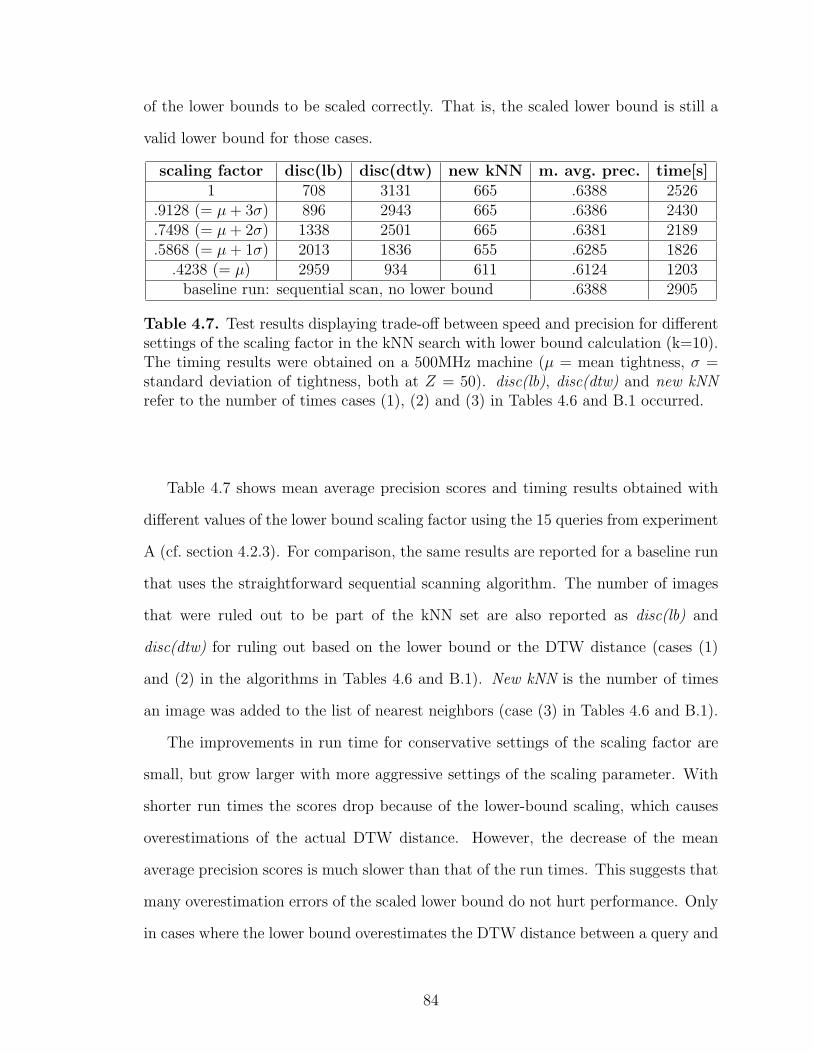
of the lower bounds to be scaled correctly. That is, the scaled lower bound is still a

valid lower bound for those cases.

scaling factor disc(lb) disc(dtw) new kNN m. avg. prec. time[s]1 708 3131 665 .6388 2526

.9128 (= µ + 3σ) 896 2943 665 .6386 2430

.7498 (= µ + 2σ) 1338 2501 665 .6381 2189

.5868 (= µ + 1σ) 2013 1836 655 .6285 1826.4238 (= µ) 2959 934 611 .6124 1203

baseline run: sequential scan, no lower bound .6388 2905

Table 4.7. Test results displaying trade-off between speed and precision for differentsettings of the scaling factor in the kNN search with lower bound calculation (k=10).The timing results were obtained on a 500MHz machine (µ = mean tightness, σ =standard deviation of tightness, both at Z = 50). disc(lb), disc(dtw) and new kNNrefer to the number of times cases (1), (2) and (3) in Tables 4.6 and B.1 occurred.

Table 4.7 shows mean average precision scores and timing results obtained with

different values of the lower bound scaling factor using the 15 queries from experiment

A (cf. section 4.2.3). For comparison, the same results are reported for a baseline run

that uses the straightforward sequential scanning algorithm. The number of images

that were ruled out to be part of the kNN set are also reported as disc(lb) and

disc(dtw) for ruling out based on the lower bound or the DTW distance (cases (1)

and (2) in the algorithms in Tables 4.6 and B.1). New kNN is the number of times

an image was added to the list of nearest neighbors (case (3) in Tables 4.6 and B.1).

The improvements in run time for conservative settings of the scaling factor are

small, but grow larger with more aggressive settings of the scaling parameter. With

shorter run times the scores drop because of the lower-bound scaling, which causes

overestimations of the actual DTW distance. However, the decrease of the mean

average precision scores is much slower than that of the run times. This suggests that

many overestimation errors of the scaled lower bound do not hurt performance. Only

in cases where the lower bound overestimates the DTW distance between a query and

84

a matching candidate, a loss in performance occurs because the candidate is falsely

discarded. The small decrease in mean average precision scores for more aggressive

settings of the scaling parameter indicates that most of the overestimation errors

occur when non-matching candidates are compared to the query. When taking the

preprocessing time into consideration, the fastest matching run is about twice as fast

as the baseline run, with about 2.6% loss in mean average precision – an acceptable

trade-off.

Keogh’s bound and our multivariate extension of it have not been the last devel-

opments in this area. For example, Zhu & Shasha [126] have presented a lower bound

that is tighter. So far, the speedup of nearest neighbor searches has been modest in

the word image domain. Unfortunately, the analysis of large collections of handwrit-

ten documents with the word spotting approach must be deemed infeasible in the

near future, considering the currently available processing power. With a matching

time of roughly one second for a pair of word images, a collection of 2381 word images

(10 page images), and a speedup-factor of 20, computing a sparse distance matrix

takes about 3 days on a 500MHz machine. The discrete probabilistic annotation

model (DPA) that is described in chapter 6 can process a collection of ∼250,000 word

images (1000 pages) in roughly 10 days on the same machine, without any optimiza-

tions. The CPA annotation model, which is an extension of DPA to continuous-space

feature vectors (and is also described in chapter 6), runs even faster.

4.4 Word Image Clustering Experiments

All of the previous work on word spotting has concentrated mostly on finding

effective similarity measures for word image matching, but the clustering of word

images has not been tackled. In this section, we perform word image clustering

experiments, followed by simulated cluster annotations that are designed to imitate

a human annotator.

85

Before we start clustering, we need to get a good estimate of the number of

clusters that our data will form. Heaps’ law, an empirical rule, provides the tool for

the estimation, which is discussed in the following section. With an accurate cluster

estimate we then move on to various clustering techniques that we apply to group

word images.

4.4.1 Heaps’ Law

Many clustering algorithms often require that the number of clusters to be created

is known. In fact, all of the clustering algorithms that were used in our experiments

require the target number of clusters as an input parameter. In the ideal case, each

cluster contains all instances of a particular word, so there are as many clusters as

there are distinct words in the collection at hand. In other words, the number of

clusters is equivalent to the vocabulary size.

Early work in information retrieval by Heaps [32] provides an empirical estimate

for the vocabulary size of a collection from the size of the collection in words. The

rule, which is known to be quite effective [3], has become known as Heaps’ law. It

predicts that the vocabulary size of a collection of n words can be estimated to be

V (n) = K · nβ, (4.16)

where K and β are parameters that depend on the language of the collection.

We estimated K and β by fitting Heaps’ law to the ground truth transcription of

a collection of 100 pages (21324 word images) from George Washington’s letters that

does not include our test set on which we performed clustering experiments. In order

to simulate a document of size n, we used the first n words from the transcription.

We varied n from 1 to 21324 in steps of 1, determined the vocabulary size for each

n, and then fitted Heaps’ law to the resulting curve. Figure 4.12 shows a plot of the

vocabulary size V as a function of n and the fitted curve.

86

0 0.5 1 1.5 2x 10

4

0

500

1000

1500

2000

2500

3000

3500

collection size n [words]

voca

bula

ry s

ize

V

actual vocabulary sizeHeaps’ law fit

Figure 4.12. Actual vocabulary size as a function of the collection size and a fit ofHeaps’ law shown for collection sizes of up to 21324 words.

The fitting was performed with the “Nelder-Mead” optimization procedure [52],

which minimizes the sum of squared differences between the actual vocabulary sizes

and the ones predicted by Heaps’ law. For the collection at hand, we estimated the

optimal parameter settings to be K = 7.2416 and β = .6172, resulting in a tight fit.

#Images Voc. size Predicted Voc. size Est. error4856 1209 1365 13%

Table 4.8. Accuracy of the vocabulary size prediction (with Heaps’ law).

We used these parameters to estimate the vocabulary size of a collection of 20

pages (4856 word images), our testbed for the clustering experiments. Table 4.8

shows the accuracy that Heaps’ law achieves when predicting the vocabulary size of

the testbed. Heaps’ law overestimates by 13%, which appears acceptable considering

the small size of the collection. It is also possible that a larger text source for the

parameter estimation could yield better prediction results.

87

4.4.2 Clustering

With the desired number of clusters at hand we can now turn to grouping word

images based on pairwise similarity and then determine the accuracy of the generated

clusters. Our experiments were performed using three different data sets derived from

the above testbed of 20 pages. The main difference between them lies in the features

that are used for the representation:5

Dataset A: This set uses a representation consisting of 27 features. These are 21

DFT coefficients extracted from profiles, as well as 6 scalar features. This

dataset is the same as was used in the recognition experiments described in [58].

We use it here to provide a basis for comparing word spotting with handwriting

recognition.

Dataset B: This set uses a feature representation that solely consists of DFT coeffi-

cients extracted from profiles; no scalar features were used. 33 DFT coefficients

were used to represent each word image, which is the optimal number that was

determined for this dataset (see section 3.2.2)

Dataset C: This dataset does not consist of feature vectors, but rather of a 4860×

4860 sparse matrix with pairwise distances. The distances were calculated using

the Dynamic Time Warping word matching algorithm described in section 4.2.2

above. The matrix is sparse, because pairwise distances were only calculated

if a word image pair was not ruled out by pruning. 76% of the matrix entries

were not computed and were filled with the default distance value infinity. The

calculation of the distance matrix required roughly one week on a multiprocessor

machine with 4 500MHz CPUs.

5Due to a small number of annotation mistakes in dataset A, which were later corrected, datasetsB and C are slightly larger (4860 word images) than dataset A (4856 word images).

88

We experimented with both the k-means clustering algorithm and various agglom-

erative clustering approaches on all data sets with one exception: since dataset C is

not represented in feature space, but rather in terms of pairwise distances, k-means

clustering cannot be applied. k-means keeps track of cluster centers, a notion that

does not exist in pairwise distance space.

Numerous clustering techniques are described in the literature. The following

is a brief overview of the clustering approaches that were used in our experiments.

More detailed descriptions of clustering techniques can be found in the relevant liter-

ature, e.g. [31]. Except for k-means clustering, all others techniques are agglomerative

bottom-up procedures, which build a hierarchical cluster tree by successively linking

the most similar clusters. For such clustering techniques, we only list how inter-cluster

dissimilarity is determined:

k-means: The algorithm is initialized with k randomly selected cluster centers. Then

each feature vector is assigned to the nearest cluster, and the cluster centers are

recalculated. This procedure is repeated until convergence.

Single linkage: The inter-cluster dissimilarity between two clusters is the distance

between the closest items within the two clusters.

Complete linkage: The distance between the two furthest items in the clusters is

used as the cluster dissimilarity.

Average linkage: Here the distance between two clusters is the average distance

between all item pairs in the clusters.

Weighted linkage: A slight variation of the Average Linkage technique, which uses

a weighted average for the cluster distance calculation.

Ward linkage: This linkage uses the sum of squares measure to assess the similarity

between clusters. The sum of squares is the total squared distance of all items

89

in a cluster relative to the cluster centroid. The distance between two clusters

is then taken to be the increase in the sum of squares measure, before and after

joining the clusters.

Each of our experiments involves selecting a dataset and a clustering method.

First, the desired number of clusters is estimated using Heaps’ law. Then, we start

the clustering of the data. In the case of k-means clustering, the feature vectors form

the input for the clustering algorithm. All other clustering routines use a dendrogram

as input, which may be constructed from pairwise distances between word images or

their feature vectors. We used the Euclidean distance measure to calculate distances

between feature vectors.6 The output of the clustering is a vector of cluster labels,

which assigns each word image to a single cluster.

The accuracy of a particular clustering output is evaluated by simulating the task

of labeling clusters, which would be performed by a human annotator if we were

to perform word spotting. For the purpose of the simulation, it is assumed that a

human annotator would label a cluster with the vocabulary term that occurs most

frequently in a cluster. This strategy is sound, because it minimizes the total number

of wrong annotations, when cluster labels are spread over all word images within a

cluster. Ground truth data is available for all word images, so this process may be

easily simulated. Once all clusters have been annotated in this fashion, we assign

each cluster label to all word images within the cluster, essentially transcribing the

entire collection. Table 4.9 shows the word error rates of such transcriptions obtained

from various clustering approaches.

Again, we can observe the importance of good features: the clustering tends to

perform better on data sets B and C, although all sets were derived from the same

20 pages. Data set B yielded the best overall result, with Ward linkage clustering.

6Certain clustering algorithms (e.g. the Ward linkage) only produce meaningful output if thevector distances are Euclidean.

90

Clustering algorithm A: WER B: WER C: WERk-means 64.13% 41.58% n/aSingle linkage 62.93% 65.10% 65.00%Complete linkage 58.55% 37.24% 36.11%Average linkage 58.44% 44.47% 34.12%Weighted linkage 58.24% 41.03% 34.77%Ward linkage 58.18% 31.50% 34.47%

Table 4.9. Performance of the clustering algorithms in terms of word error rate(WER), after simulated annotation of the entire collection.

Interestingly, the DTW dissimilarity data (set C) performs slightly worse than the

best result (Ward linkage on set B), but otherwise consistently better than set B with

word error rates between 34% and 36% (except for the single linkage algorithm). This

suggests that the DTW distance measure captures different aspects of word image

similarity than the features used in set B. The difference in performance between

sets B and C can be attributed to the fact that the length of the feature vectors

in set B (number of DFT coefficients) has been optimized for this exact dataset,

yielding better performance. Furthermore, the matrix with DTW distances has not

been entirely computed due to pruning, which probably has an adverse effect on

performance (the pruning assigns infinity as the distance to some word image pairs).

However, the magnitude of this effect is unknown.

Figure 4.13 shows histograms of the sizes of clusters that have been generated

with the best performing methods on sets B and C (average linkage and Ward linkage

respectively), as well as the output of a clustering technique with higher word error

rate (k-means on set B). The clustering techniques with lower word error rate are a

better match for the actual distribution of cluster sizes. This is also true of techniques

for which no plots are provided. It is important for a good clustering approach to

produce clusters of a variety of sizes. The output of the k-means clustering in Figure

91

4.13(d) shows that clusters which should have been large, were broken down into

smaller pieces.

0 10 20 30 40 500

100

200

300

400

500

600

700

800

cluster size

frequ

ency

(a) From ground truth (sets B &C).

0 10 20 30 40 500

100

200

300

400

500

600

cluster size

frequ

ency

(b) Set C, average linkage clusters.

0 10 20 30 40 500

100

200

300

400

500

cluster size

frequ

ency

(c) Set B, Ward linkage clusters.

0 10 20 30 40 500

50

100

150

200

250

300

350

cluster size

frequ

ency

(d) Set B, k-means clusters.

Figure 4.13. Histograms of perfect and automatically determined cluster sizes. Someclustering algorithms achieve a good match to the actual cluster size distribution(b),(c), while others tend to produce clusters with a limited range of sizes (d). Asmall number of clusters with sizes greater than 50 has been omitted from (a) and(c) to allow the displaying of all histograms on the same x-scale.

Our goal is not to obtain labels for all word images in the collection. Following

Luhn’s line of thought, we can identify clusters that should make good candidates

for an index. We constrained the simulated annotation to clusters with at least 3

members, but not more than 50, and calculated the word error rate for the simulated

annotation that is restricted only to the selected clusters. Table 4.10 contains the

92

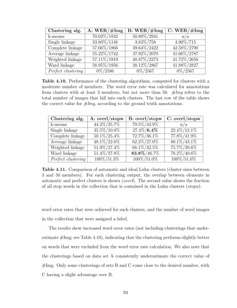
Clustering alg. A: WER/#Img B: WER/#Img C: WER/#Imgk-means 70.03%/1832 50.80%/2941 n/aSingle linkage 33.80%/1148 3.83%/758 4.90%/715Complete linkage 57.66%/1866 39.64%/2422 42.58%/2790Average linkage 55.22%/1742 37.92%/2070 41.66%/2787Weighted linkage 57.11%/1919 40.87%/2273 41.72%/2656Ward linkage 58.95%/1956 38.12%/2867 41.88%/2827Perfect clustering 0%/2586 0%/2567 0%/2567

Table 4.10. Performance of the clustering algorithms, computed for clusters with amoderate number of members. The word error rate was calculated for annotationsfrom clusters with at least 3 members, but not more than 50. #Img refers to thetotal number of images that fall into such clusters. The last row of the table showsthe correct value for #Img, according to the ground truth annotations.

Clustering alg. A: overl/stopw B: overl/stopw C: overl/stopwk-means 44.2%/25.7% 79.5%/43.9% n/aSingle linkage 35.5%/10.0% 27.4%/6.4% 22.4%/12.1%Complete linkage 50.1%/25.4% 72.7%/36.1% 77.8%/41.9%Average linkage 48.1%/22.6% 62.2%/27.0% 80.1%/43.1%Weighted linkage 51.9%/27.4% 68.1%/32.5% 75.7%/39.6%Ward linkage 51.4%/27.8% 83.8%/46.7% 78.2%/40.6%Perfect clustering 100%/51.3% 100%/51.0% 100%/51.0%

Table 4.11. Comparison of automatic and ideal Luhn clusters (cluster sizes between3 and 50 members). For each clustering output, the overlap between elements inautomatic and perfect clusters is shown (overl). The second value shows the fractionof all stop words in the collection that is contained in the Luhn clusters (stopw).

word error rates that were achieved for such clusters, and the number of word images

in the collection that were assigned a label.

The results show increased word error rates (not including clusterings that under-

estimate #Img; see Table 4.10), indicating that the clustering performs slightly better

on words that were excluded from the word error rate calculation. We also note that

the clusterings based on data set A consistently underestimate the correct value of

#Img. Only some clusterings of sets B and C come close to the desired number, with

C having a slight advantage over B.

93

The cluster selection based on the single linkage clustering produces small word

error rates, but this clustering approach performs poorly. The selected number of

clusters is substantially lower than the target number, which is the cause of the low

word error rates. The word error rates that can be expected from the word spotting

approach should be taken from clusterings that produce better matches in terms of

the desired number of clusters, e.g. the weighted linkage technique on data set C.

Table 4.11 shows the amount of overlap (overl) between the members contained

in automatic and perfect (from ground truth) Luhn clusters. The overlap is high

for clustering techniques that yielded low word error rates and a good match of

#Img (cf. Table 4.10), e.g. the Ward linkage technique on data set B or the average

linkage method on data set C. The second reported value (stopw) in Table 4.11 is

the fraction of all stop words in the collection that is contained in Luhn clusters.

Somewhat surprisingly, all automatic clusterings contain a smaller fraction of all stop

words than the perfect clustering. This is expected for clusterings that substantially

underestimate #Img (all clusterings of data set A and all single linkage clusterings).

For the remaining clustering techniques, it seems that our Luhn cluster selection

approach (selecting clusters with sizes between 3 and 50 members) works better for

automatic clusterings than for the perfect clustering based on ground truth data. The

large fractions of stop word content in the clusters also suggest that a more restrictive

selection of Luhn clusters may be used.

Word spotting appears as an attractive alternative to the seemingly obvious recog-

nize-then-retrieve approach to historical manuscript retrieval. With the capability to

match word images quickly and accurately (e.g. using Euclidean distance between

feature vectors), partial transcriptions of a collection can be obtained with reason-

able accuracy and little human intervention. Because of the general complexity of

the problem, however, which is O(n2) for datasets with n word images, very large

datasets remain out of reach in the near future. Word spotting has the capability to

94

automatically identify indexing terms, making it possible to use costly human labor

more sparingly than a full transcription would require. For example, using the Ward

linkage clustering on data set B, it would be possible to obtain 2867 word image labels

with a word error rate of 38.12%, by annotating just 291 clusters (cluster sizes be-

tween 3 and 50 members). That is, the word spotting procedure would have reduced

2867 annotations to about 10% of that. Even greater savings (in terms of percent)

can be expected from larger collections, since vocabularies grow sublinearly in the

size of the corresponding collections.

95

CHAPTER 5

RECOGNITION AND RETRIEVAL

Traditionally, information retrieval has been performed on electronic representa-

tions of text, e.g. document encodings in ASCII. The quality of retrieval systems for

such documents has led to widespread use and commercial success. It is only natural

to attempt to recognize the text in historical manuscript images, and then perform

retrieval on the resulting automatic transcription. Here we describe our work on rec-

ognizing historical manuscripts, and take a look at the retrieval quality that can be

achieved with the automatic recognition output.

5.1 Hidden Markov Document Model

In [58] a holistic recognition approach for handwritten historical documents was

presented. It uses a Hidden Markov Model (HMM) [86] to describe the creation

process of a document, which is represented as an ordered sequence of handwritten

words (see Figure 5.11). At each position i in the document, the author decides

to write a particular word wi, which is chosen based only on the word wi−1 at the

previous position. Depending on the word choice wi, a feature vector fi is chosen.

We assume that the feature vector entirely determines the visual appearance of the

writing. This allows us to use the fi as our observations in place of the actual word

images, when we recognize a sequence of word images.

1We use upper-case characters to denote random variables, lower-case characters denote observedvalues.

96

Figure 5.1. Hidden Markov Model of the document creation process. The documentis modeled as a hidden sequence of handwritten words Wi, where each written wordonly depends on the word in the previous state. Based on the word choice Wi at po-sition i, a feature vector Fi is randomly sampled from a word-conditional distributionP (Fi|Wi).

During recognition, a sequence of continuous-space feature vectors fi (as described

in section 3.1) is given, and the task is to infer the values of the hidden state vari-

ables Wi from the features. Each random state variable Wi takes on values from a

vocabulary V (e.g. all English words), so the output of the recognition process is a

sequence of words.

The main distributions that are needed to specify an HMM are the conditional

feature distributions P (Fi|Wi) and a transition probability distribution P (Wi|Wi−1).

We assume all of them to be stationary, so we omit the index i where possible. In

the following sections, we describe the models for the feature generation and how the

transition probabilities were obtained.

5.1.1 Observation Model

We assume a multivariate normal density for the conditional feature distributions

and use annotated training data T to estimate the parameters. For a given word

w ∈ V , the likelihood of observing the d-dimensional feature vector f as its feature

vector is taken to be

97

p(F = f |W = w) =exp

{−1

2(f − µw)>Σ−1(f − µw)

}√2dπd|Σ|

, (5.1)

where µw is estimated from the training instances Tw for w and Σ from the entire

training data:

µw =1

|Tw|∑f∈Tw

f ,

Σ = I · σ2 = I · 1

d

d∑p=1

(1

|T | − 1

∑f∈T

(fp − µT ,p)2

),

where p is used to index dimensions and

Tw = {fi ∈ T |wi = w},

µT =1

|T |∑f∈T

f .

We constrain our conditional feature distribution to take the form of an isotropic

Gaussian density. The covariance matrix Σ is the same for all states W = w, because

its parameters can be estimated more reliably. The small size of our training collection

T would otherwise yield unreliable estimates for Σ.

For consistency with prior publications (e.g. [58]), all of the word images in the

experiments in this chapter were represented with 27-dimensional feature vectors

consisting of 6 scalar features, such as the word image width, and 21 DFT coefficients

that were extracted from profile features (see sections 3.1.1 and 3.2.1).

5.1.2 Transition Model

The transition probability distribution corresponds to a word bigram frequency

distribution over the considered vocabulary V that is usually represented as a stochas-

tic table. It can be estimated from the training data and additional text corpora. In

98

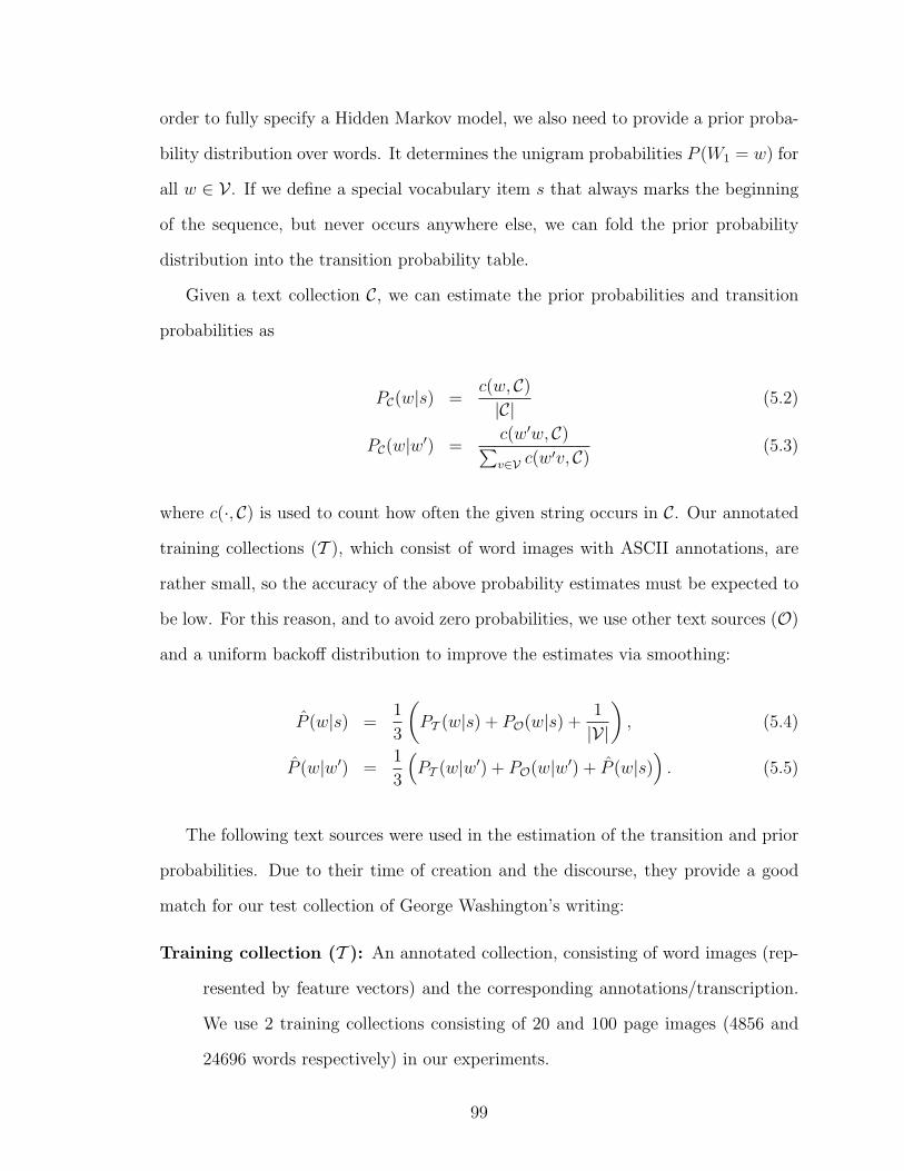
order to fully specify a Hidden Markov model, we also need to provide a prior proba-

bility distribution over words. It determines the unigram probabilities P (W1 = w) for

all w ∈ V . If we define a special vocabulary item s that always marks the beginning

of the sequence, but never occurs anywhere else, we can fold the prior probability

distribution into the transition probability table.

Given a text collection C, we can estimate the prior probabilities and transition

probabilities as

PC(w|s) =c(w, C)

|C|(5.2)

PC(w|w′) =c(w′w, C)∑v∈V c(w′v, C)

(5.3)

where c(·, C) is used to count how often the given string occurs in C. Our annotated

training collections (T ), which consist of word images with ASCII annotations, are

rather small, so the accuracy of the above probability estimates must be expected to

be low. For this reason, and to avoid zero probabilities, we use other text sources (O)

and a uniform backoff distribution to improve the estimates via smoothing:

P (w|s) =1

3

(PT (w|s) + PO(w|s) +

1

|V|

), (5.4)

P (w|w′) =1

3

(PT (w|w′) + PO(w|w′) + P (w|s)

). (5.5)

The following text sources were used in the estimation of the transition and prior

probabilities. Due to their time of creation and the discourse, they provide a good

match for our test collection of George Washington’s writing:

Training collection (T ): An annotated collection, consisting of word images (rep-

resented by feature vectors) and the corresponding annotations/transcription.

We use 2 training collections consisting of 20 and 100 page images (4856 and

24696 words respectively) in our experiments.

99

Jefferson collection (O1): These transcriptions (200,000 words) are part of the

Jefferson corpus at the Library of Congress.

Washington collection (O2): A large corpus (4.5 million words) consisting of tran-

scriptions that were obtained from the Library of Congress [110]. We excluded

portions from this corpus that were used for testing.

Based on these collections, we calculate various unigram and bigram distributions to

test the effect of increasingly accurate probability estimates on the recognition error

rate. We describe these distributions and the results in the experiments section.

5.1.3 Recognition with Hidden Markov Models

Recognition may be loosely described as finding the state sequence w1 . . . wN that

best explains the observation sequence f1 . . . fN . Several solutions are possible, each

optimizing a different quantity. For example, we could seek to optimize the likelihood

of each state individually given the observations, which would maximize the expected

number of correct states [86]. However, this may lead to state sequences that are

impossible according to the state transition model (e.g. the word pair the the might

be considered an invalid state sequence).

Since the goal of recognition is often to create a readable transcription of a docu-

ment, we will recover the state sequence that jointly maximizes the likelihood of the

observation sequence. This sequence may be determined with the Viterbi algorithm

[25, 86], a dynamic programming technique. The algorithm recursively calculates

δi(w) = maxw1...wi−1

P (W1 . . . Wi = w, f1 . . . fi)

using the recursion

δi+1(w) =(

maxw′

δi(w′) · P (Wi+1 = w|Wi = w′)

)· P (Fi = fi|Wi = w) (5.6)

and the initial condition

δ1(w) = P (W1 = w) · P (F1 = f1|W1 = w).

100

When δi(w) has been computed for all pairs of i and w, the algorithm tracks back the

most likely state sequence, starting from the state wN in the trellis defined by δi(w):

wN = argmaxw

δN(w).

From there, backtracking determines all arguments w that yielded the maximum value

in equation (5.6). The algorithm terminates when the backtracking has determined

the most likely state at position 1 in the sequence.

5.1.4 Recognition Experiments

Our recognition and retrieval experiments were conducted on three datasets. All

datasets were first segmented automatically, and then corrected by a human annota-

tor, who also supplied annotations that we use as ground truth for the evaluation of

the recognition and retrieval results:

Dataset A: A dataset consisting of 20 page images (4856 word images2) from the

George Washington collection.

Dataset B: 100 page images (24696 word images) from the Washington collection.

dataset A is entirely contained in this set.

Dataset C: 100 page images (21324 word images) from the Washington collection.

Due to their larger size, datasets B and C have not received the same level of human

attention. This causes these datasets to be less accurate in the sense that word

segmentation coordinates are not as accurate and some ground truth annotations are

incorrect. On the other hand, we believe dataset A to be almost free of such mistakes.

2The number of word images may be slightly different from other published results, because of asmall number of corrections that have been made to the dataset.

101

5.1.4.1 Influence of Transition Model

Our first recognition experiment was performed entirely on dataset A, using 20-

fold cross validation: 19 annotated pages were used for training the bigram (tran-

sition) and observation probabilities, and the remaining page was recognized using

the above HMM recognizer. Since the recognition is performed at word-level, only

terms that occur in the training data can be recognized. Terms that occur in the test

document, but not in the training documents are called Out-Of-Vocabulary (OOV)

terms.

The supplemental Washington and Jefferson collections that were downloaded

from the Library of Congress were used to estimate various unigram and bigram

models, which are listed here. Whenever a text source (T and/or O) is not used in

the estimation, the mixing weights in equations (5.4,5.5) need to be adjusted:

Uniform: No text source is used, all state transitions are equally likely.

Unigram: Only uses T for the estimation of the unigram frequencies. The unigram

frequencies are used in place of bigram estimates: P (w|w′) = P (w|s).

19 pages: Both bigrams and unigrams are estimated only from the pages that make

up the training set. No other (O) text sources are used.

19+Jeff: The estimation uses the training pages as T and the Jefferson pages as other

text sources (O = O1). The probability estimation is exactly as in equations

(5.4,5.5).

19+J+W: Same as above, but O is made up of the union of the downloaded Jefferson

and Washington transcriptions (O = O1 ∪ O2).

Target: The bigrams are estimated from the page to be recognized. This is a cheating

experiment that can be used to compute an upper bound on the recognition

performance.

102

Table 5.1 shows the achieved word error rates for each of the above unigram and

bigram estimates. Each error rate in the table is the average over 20 cross-validation

runs. The analysis was performed both with and without considering OOV terms,

yielding lower error rates when OOV terms are excluded.

Bigram Model Word Error RateSource Size Excluding OOV Including OOVUniform 0 53.1% ± 5% 60.3% ± 5%Unigram 4.6K 44.8% ± 5% 53.3% ± 5%19 pages 4.6K 41.4% ± 6% 50.3% ± 7%19+Jeff 191K 38.8% ± 5% 48.1% ± 6%

19+J+W 4,533K 34.9% ± 6% 44.9% ± 7%Target 243 4.5% ± 3% 6.3% ± 4%

Table 5.1. Word error rates for handwriting recognition with a word-level HiddenMarkov Model, using bigram estimates from collections of varying sizes. The analysiswas performed both excluding and including Out-Of-Vocabulary words in the errorrate calculation.

The beneficial effect of using large text sources for the estimation of the transition

models can be seen very clearly. The word error rates (WER) drop substantially

from 53% to 35% without considering OOV terms, when moving from a transition

model that considers no text source at all, to a model that uses a large collection

of text from the same time period and about approximately the same topic as the

recognized text. Still, the error rates are generally high, and would be unacceptable

to a human reader. They are, however, comparable to other results reported in the

literature, which range from about 40% to 63%. These numbers were obtained on

modern documents of high quality with vocabulary sizes from 525 to 7719 [46, 83].

The vocabulary size of test set A is 1187.

Not surprisingly, the lowest word error rate was achieved with the bigram model

estimated from the page that is to be recognized. The large difference in performance

compared to that of the second-best bigram model suggests that much improvement

could be expected from further improvement of the transition model. This would

103

require even more text sources that are relevant to the collection to be recognized.

However, since our documents are historical, such data is not readily available in

electronic text formats.

Comparing the recognition results with those obtained from simulated annotation

results on clustered word images shows the competitiveness of the word spotting tech-

nique. With all clusters annotated, word spotting has a word error rate of 34.12%

using the average linkage clustering method and the DTW distance measure. This

would require only 1365 cluster annotations (for a total of 4856 annotated word im-

ages), compared to roughly 4600 training annotations in the above recognition exper-

iments for a total of 240 automatic word image annotations on one recognized page.

When the collection of clusters is further limited by only annotating “interesting”

clusters (cluster sizes between 3 and 50 members), word spotting still outperforms

the best HMM recognition results including OOV terms with 41.66% WER versus

44.9%. In this case, only 278 cluster annotations need to be provided. However, the

computational demands of the word spotting approach make the HMM recognition

approach more desirable for large datasets.

5.1.4.2 Recognition of Large Datasets

The above experiment was performed on a small dataset. Only one page image

was recognized, which is very little data (there are about 240 words per page on

average) for assessing retrieval performance. Here we describe our recognition results

on dataset C (100 pages), which is much better suited for this task. For training,

datasets A (20 pages) and B (100 pages) were used.

The test set was recognized using two methods:

HMM: The Hidden Markov Model recognition approach described above.

BDT: A classification technique for word images that uses boosting to build an

ensemble classifier from individual decision tree classifiers that operate on multi-

104

resolution bitmap representations of word images. The approach was described

in [35]; we use the recognition output here for comparison.

Since we are recognizing George Washington’s handwritten letters, we only used the

training data and the Jefferson transcriptions in the estimation of the transition model

for the HMM approach. Using all of the transcriptions that are available for George

Washington’s letters would result in a very good bigram model, but it is unrealistic to

assume that such closely matching text sources are available in an actual recognition

situation. The BDT classifier does not use the bigram language model.

Evaluation technique A/HMM A/BDT B/HMMWER (including OOV terms) 66.60% 55.83% 69.86%WER (excluding OOV terms) 54.83% 39.51% 64.47%Recognition vocabulary size 3722 3738 5980

Table 5.2. Word error rates (WER) and vocabulary sizes used in the recognition.The vocabulary sizes of the A/HMM and A/BDT experiments vary slightly, becausea small number of corrections have been made to dataset A over time (A/BDT usesthe most recent version).

Table 5.2 shows the word error rates we obtained with the above recognizers us-

ing datasets A and B for training. A/BDT clearly outperforms both A/HMM and

B/HMM in terms of word error rate by a wide margin of more than 10%. However,

we will see shortly that the superior performance of A/BDT does not necessarily

translate into better retrieval performance. Somewhat surprisingly the error rate of

B/HMM, which uses a much larger training set, is worse than that of A/HMM. Nor-

mally, one would expect a larger training set to yield better results. In this case,

however, increasing the training set size comes with a significantly increased vocabu-

lary (3722 to 5980). This makes classification harder, because of the increased number

of categories that the recognizer is presented with. Large-vocabulary documents are

the real challenge when performing handwritten document recognition. The cross-

modal retrieval approach based on continuous features we present in chapter 6 does

105

not immediately suffer from this drawback. We show that its performance increases

when a larger training set is used. The reason lies in its approach to classification,

which avoids making hard decisions (as recognizers do).

5.2 Retrieval

We now use the recognition output and perform retrieval on it. To do this, the

automatically generated transcription of a page image is treated as an electronic

document, just as a manually generated transcription would be. We can then select

a retrieval model and run experiments to test the retrieval performance.

5.2.1 Language Model Retrieval

A retrieval model specifies how documents are ranked in response to a query. For

our experiments, we chose the language model retrieval approach [85], because it is

well adapted to situations with probabilistic document representations. This fact

makes language model retrieval particularly attractive for the probabilistic retrieval

approaches in chapter 6. We use the same retrieval model here for comparability.

In language model retrieval, each document is represented by a probabilistic model

that captures occurrence frequencies of terms in the document. Such document models

can be used to calculate the probability of observing a particular combination of

words when selecting terms from a document at random. Ponte and Croft [85] used

the probability of observing a given query as a random sample from a document

model MD as the score for the document D. We will call this scoring function the

query-likelihood approach in the following.

The original proposed language model retrieval advocated Bernoulli document

models, but multinomial models [105] are now a more popular choice. With this

model, the probability of sampling the query Q = w1 . . . wk from the document model

MD may be calculated as

106

P (Q|MD) =k∏

i=1

P (wi|MD), (5.7)

where P (wi|MD) = c(wi,D)|D| is the maximum-likelihood estimate of the term frequency

in the document D. In practice, the term frequency estimates are often smoothed

with the collection frequencies, to avoid situations where a single query term with

0-frequency would cause a document to be assigned a score of 0 (see section 6.2.1 for

smoothing with the Jelinek-Mercer approach).

5.2.2 Retrieval Experiments

Dataset C was used as the test collection for all retrieval experiments. Its size

allows us to use it both for line retrieval (3336 lines) and document retrieval (100

pages/documents).

Each retrieval experiment involves grouping the word annotation results of the

recognizer into retrieval units (either pages or lines, referred to as “documents” in

the following). The resulting units are then stemmed using the Krovetz stemmer [50]

and placed into an index. We selected a total of 400 queries, ranging from 1 to 4

words in length (100 queries for each query group). The query terms were sampled at

random from all lines in the test set, to ensure that at least one relevant item exists

for each query (see Table 5.3 for the number of relevant items per query group). Stop

words and terms that did not occur in the training set were excluded from the query

selection. This query set is also used in the evaluation of other retrieval techniques

(see chapter 6).

Query length 1 word 2 words 3 words 4 wordsPage retrieval 1453 625 471 203Line retrieval 2193 192 232 118

Table 5.3. Number of relevant items per query group.

107

During retrieval, each query was used to rank the documents in the collection with

the query-likelihood method. The smoothing parameter that controls the interpola-

tion between the foreground and background term probability estimate, was set to

0.8, i.e. giving more weight to foreground term probability estimates. The resulting

ranked lists were evaluated using the trec eval program. A retrieved item was judged

relevant to a query, if it contains each of the query terms at least once. Table 5.4

shows the mean average precision (MAP) scores that were achieved for retrieval on

dataset C, with training sets A and B, using the HMM and BDT recognition model.

The best result in each row was compared to the other results using the sign test [26].

If there was a statistically significant difference (significance level α = .05), the lower

result was marked with an asterisk (∗).

Exper. Query len. A/HMM A/BDT B/HMM1 word .1818 .1676 .1623

Page 2 words .2451 .2293 .1984∗retrieval 3 words .2777 .2481 .2097∗

4 words .3874 .3410∗ .2200∗1 word .0933 .1018 .0826

Line 2 words .1655 .1603 .1175retrieval 3 words .2630 .2466 .1312∗

4 words .2903 .3766 .1394∗

Table 5.4. Mean average precision scores for the retrieval experiments conducted onautomatically recognized pages. Each column shows results obtained with a particulartraining set (A or B) and recognition approach (HMM or BDT). Results that aresignificantly different from the best result in each row are marked with an asterisk(∗).

Surprisingly, despite its substantially better recognition performance (cf. Table

5.2), the BDT technique does not yield the best retrieval performance. The HMM

recognizer on dataset A outperforms or matches BDT’s results, except for line retrieval

with queries of length 4. It seems that the lower word error rates achieved with BDT

have to be attributed to terms that are not used in queries, for example stop words.

108

In fact, it turns out that the WER for words on a standard stop word list is 28.70%

(using the BDT recognizer), while the WER of non-stopwords is 82.33%.

Another reason for the difference in performance could be the length of the re-

turned ranked list. Our test collection is rather small when compared to corpora that

are typically used in information retrieval of text (e.g. TREC collections). This can

have effects on the evaluation of ranked result lists, which typically are not observed

in large collections. The reason lies in the trec eval program, which assigns a precision

of 0 to relevant items that do not occur in a ranked result list. When working with

large collections, typically the top 1000 documents are returned, and relevant docu-

ments that were not retrieved have a precision close to 0 (less than 10−3). However,

when the ranked result list is short, as is the case here with document retrieval and

short queries (or smoothing turned off), assigning a precision of 0 can significantly

underestimate the precision. In this situation, simply returning a longer ranked list

can improve the average precision score of a retrieval run. Since we are using smooth-

ing, queries with more terms return longer ranked lists, which result in higher average

precision scores.

Exper. Query len. A/HMM A/BDT B/HMM1 word .2740 .2643 .2629

Page 2 words .2574 .2405 .2208retrieval 3 words .2811 .2505 .2163

4 words .3880 .3417∗ .2228∗1 word .0979 .1062 .0878

Line 2 words .1662 .1611 .1186retrieval 3 words .2631 .2466 .1314∗

4 words .2903 .3766 .1395∗

Table 5.5. Mean average precision scores for the same experiments as in Table 5.4,calculated for ranked lists that contain all documents in the collection. Results thatare significantly different from the best result in each row are marked with an asterisk(∗).

109

In order to test if the above evaluation effect plays a role in the lower precision

scores of the BDT run (because BDT might tend to retrieve shorter result lists), we

repeated the evaluation in Table 5.4, with ranked lists that contain all documents in

the collection. The results are shown in Table 5.5. Still, the picture of the comparison

between A/HMM and A/BDT remains exactly the same: for the most part, A/HMM

performs better than A/BDT.

We can observe however, that in Table 5.5 the pattern of strictly increasing MAP

scores with longer queries (in Table 5.4) has been broken in the document retrieval

scores. It is still present in the line retrieval scores though, so there seems to be a

general tendency for higher scores when longer queries are used. We attribute this

to the query selection process, which selects queries from lines in the test set. This

causes a relevant line to be retrieved, even if the recognition output contains only one

of the query terms. The likelihood that at least one query term is contained in the

recognition output increases with longer queries, causing increased MAP scores for

longer queries.

As we would expect from its lower recognition rate, the retrieval performance of

B/HMM falls short of that of A/HMM and A/BDT. This shows – again – the chal-

lenges that recognition/annotation techniques face in the presence of large-vocabulary

applications. It has to be pointed out, however, that the query selection was per-

formed on the intersection of the vocabularies of sets A and C, to guarantee that the

same queries can be used in all experiments. A search engine built with the output of

B/HMM would allow a wider range of query terms, because its training vocabulary is

a superset of the vocabulary of set A. This fact was not considered in our evaluation

here.

Table 5.6 shows precision scores at the top 5 retrieved items for all retrieval runs.

The picture is similar to the mean average precision results in Table 5.5, with A/HMM

performing best in the page retrieval experiments. In the line retrieval experiments,

110

Exper. Query len. A/HMM A/BDT B/HMM1 word 0.3060 0.2680 0.2940

Page 2 words 0.2120 0.2080 0.1940retrieval 3 words 0.1900 0.1760 0.1640

4 words 0.1620 0.1560 0.1140∗1 word 0.1680 0.1680 0.1740

Line 2 words 0.0660 0.0660 0.0540retrieval 3 words 0.0840 0.0860 0.0560∗

4 words 0.0800 0.1120 0.0500∗

Table 5.6. Precision at the top 5 retrieved items for retrieval runs based on recogni-tion output. All ranked lists were padded to contain all documents in the collection.Results that are significantly different from the best result in each row are markedwith an asterisk (∗).

A/BDT seems to perform slightly better than the remaining techniques, although not

significantly better than A/HMM. The generally low level of the precision scores may

be explained by the small number of relevant items per query (cf. Table 5.3), which

causes the maximum achievable precision-at-5 of many queries to be substantially less

than 100%, especially for queries consisting of multiple words. Another contributing

factor to lower precision numbers are recognition errors, which cause relevant items

not to be retrieved.

Recognizers make hard classification decisions, that is, they return a single anno-

tation term for each word image on a page. In our case, that decision is based on a

probability estimate, which indicates that a particular choice is more likely to be the

answer than any of the alternatives. If the decision is made, the information about

alternatives is no longer available. This could cause a document not to be retrieved

(or at a very low rank) if a term used in the query was wrongfully dismissed by the

recognizer. In the following chapter, which uses cross-modal models for the anno-

tation of word images, we show how the information about alternative word image

annotations may be used to improve retrieval performance.

111

CHAPTER 6

CROSS-MODAL RETRIEVAL

In this chapter, we focus on retrieval with cross-modal models. These models

describe the joint occurrence of annotation words and features. Cross-media mod-

els were reported for automatic color photograph annotation and retrieval [41, 57].

Here we adapt such models for the cross-modal application of retrieving historical

manuscripts using text queries [92]. Our models can exploit the statistical regulari-

ties of language and we show how a bigram language model may be used to constrain

annotations of adjacent word images, yielding substantially improved retrieval re-

sults. In addition, our cross-modal models allow the retrieval of units of arbitrary

size (e.g. pages or lines), not just individual images as in previous work.

Cross-modal retrieval models are closely related to previous work in cross-lingual

information retrieval of text, where joint models of words in two different languages

are used to retrieve documents in a language that differs from the query language.

By analogy, word images and their annotations may also be seen as representations

of the same concept in two languages.

We present three cross-modal retrieval models for historical manuscripts, evaluate

their performance and compare them against the retrieval performance that can be

achieved on recognition output. Finally, we look at ideas on how to tackle the problem

of out-of-vocabulary terms with synthetic training data. This allows the use of such

terms in queries despite the lack of training data.

112

6.1 Joint Models for Annotation Words and Features

Cross-modal models describe the joint occurrence of annotation words and fea-

tures. We will look at annotations and features of word images and then move to

larger retrieval units. Our model describes the probability of observing a particu-

lar annotation word w together with a particular feature representation f of a word

image:

P (w, f)

We assume that w is selected from a vocabulary V (e.g. all English words) and the

feature representation f is an element of some feature space F . This model allows us

to do two things:

Probabilistic Annotation: For a given feature representation f , we can calculate

a distribution over potential annotation terms w ∈ V using

P (w|f) =P (w, f)∑v∈V P (v, f)

. (6.1)

That is, each entry in the vocabulary V is assigned a probability that it is the

correct annotation term for the given feature representation. The annotation

probabilities that occur within a retrieval unit may be used to estimate a un-

igram model for it, which is an approximation of the model that would arise

from the true term counts in the retrieval unit.

Content Modeling: For a given annotation word w, we can predict a model/distri-

bution in the feature space F that describes image content which we would like

to retrieve. That is, w can be seen as a query, which returns a distribution over

feature representations f :

P (f |w) =P (w, f)∑

g∈F P (w,g), (6.2)

113

where we assume that the feature space F is discrete. The feature distribu-

tion may then be used to score word images (their features) by their degree of

agreement with the distribution.

In chapter 3, we discussed a discrete feature representation and continuous-space

feature vectors. Depending on the feature space F , our model of P (w, f) varies.

We use the discrete feature representation for probabilistic annotation and content

modeling, and continuous-space features for probabilistic annotation, yielding a total

of three cross-modal retrieval models. We will refer to them as DPA, CPA and DCM

respectively. Before we move on to the estimation of P (w, f), we take a look at the

origin of cross-modal retrieval.

6.1.1 Cross-Lingual Text Retrieval

Cross-lingual information retrieval of text documents allows a query to be for-

mulated in one language, and the retrieved documents to be in another language.

The problem of retrieving handwritten content using English queries is analogous to

cross-lingual retrieval, if the handwritten content is described with an image descrip-

tion language. In section 3.3, we presented a discretization technique which turns

continuous-space feature vectors into feature tokens from a token vocabulary F . This

allows us to adapt cross-lingual ideas for text documents to our multimedia content.

Lavrenko et al. [53] presented an approach to cross-lingual information retrieval of

text that is based on relevance models. They assume that relevant documents and the

queries that would retrieve them are random samples from a relevance distribution.

If the relevance model RQ were known for a given query Q = e1, . . . , ek of English

words, one could use the relevance model to extract a language model P (w|RQ) in

the other language. This target language model may then be used to rank documents

in the foreign language.

114

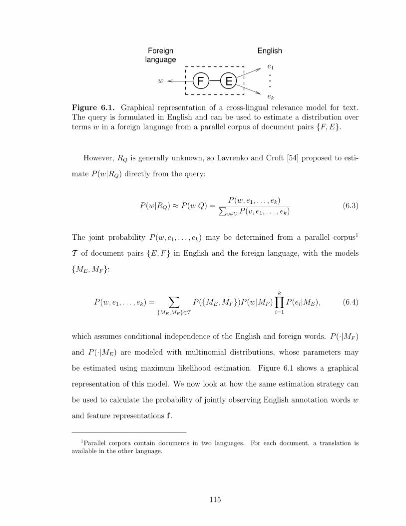
F E...

Foreignlanguage

English

e1

ek

w

Figure 6.1. Graphical representation of a cross-lingual relevance model for text.The query is formulated in English and can be used to estimate a distribution overterms w in a foreign language from a parallel corpus of document pairs {F, E}.

However, RQ is generally unknown, so Lavrenko and Croft [54] proposed to esti-

mate P (w|RQ) directly from the query:

P (w|RQ) ≈ P (w|Q) =P (w, e1, . . . , ek)∑v∈V P (v, e1, . . . , ek)

(6.3)

The joint probability P (w, e1, . . . , ek) may be determined from a parallel corpus1

T of document pairs {E, F} in English and the foreign language, with the models

{ME, MF}:

P (w, e1, . . . , ek) =∑

{ME ,MF }∈T

P ({ME, MF})P (w|MF )k∏

i=1

P (ei|ME), (6.4)

which assumes conditional independence of the English and foreign words. P (·|MF )

and P (·|ME) are modeled with multinomial distributions, whose parameters may

be estimated using maximum likelihood estimation. Figure 6.1 shows a graphical

representation of this model. We now look at how the same estimation strategy can

be used to calculate the probability of jointly observing English annotation words w

and feature representations f .

1Parallel corpora contain documents in two languages. For each document, a translation isavailable in the other language.

115

6.1.2 Cross-Modal Model

We can readily extend the cross-lingual relevance modeling idea for the purpose of

calculating P (w, f). Instead of a parallel text corpus, we use a training collection T

of word images and their English annotations. T consists of pairs {v,g} ∈ V ×Fk of

annotations and feature representations, where the integer k = 1 if F is a continuous

feature space (e.g. F = [0, 1]d) and k > 0 if F is a discrete feature vocabulary. |T |

refers to the number of training instances, that is, the number of pairs {v,g} ∈ T .

Cross-modal model

Mv Mg

Training instance: v g

Figure 6.2. Illustration of the cross-modal model for a single training instance{v,g}. The training annotation v and the feature vector g are assumed to be randomsamples from their respective distributions P (·|Mv) and P (·|Mg).

By analogy with the cross-lingual case, we get

P (w, f) =∑

{v,g}∈T

P ({Mv, Mg})P (w, f |{Mv, Mg}) (6.5)

=∑

{v,g}∈T

1

|T |P (w|{Mv, Mg})P (f |{Mv, Mg}) (6.6)

=∑

{v,g}∈T

1

|T |P (w|Mv)P (f |Mg), (6.7)

where we assume a uniform prior on the training instances. Together, Mv and Mg form

the cross-modal relevance model that the training instance {v,g} was sampled from

(see Figure 6.2). The above calculation of P (w, f) may be interpreted as a mixture

model of distributions P (w, f |{Mv, Mg}) that arise from the training instances. We

116

now show how to estimate Mv from v and Mg from g, which permits us to calculate

P (w|Mv) and P (f |Mg).

P (w|Mv) is the probability of sampling w from the annotation model Mv. Ob-

serving any annotation other than v should be impossible, since v is the only correct

annotation for the training instance {v,g}.2 Therefore we set

P (w|Mv) =

1 if v = w

0 otherwise

(6.8)

We assume the training feature vector g is a random sample from the distribution

P (·|Mg). If handwriting were a process that is executed with mechanical precision

and would always yield the same result, we could use a similarly restricted probability

calculation for P (f |Mg) as in equation (6.8). However, this is not the case and we

would like to assign non-zero probabilities even when f is not exactly the same as g.

Depending on the type of feature representation, we can achieve this in two ways:

1. If F is a vocabulary of discrete feature tokens as described in section 3.3, we have

f = (f1, . . . , fk) and g = (g1, . . . , gk). We treat g as a document and estimate

the distribution P (·|Mg) that it was sampled from, assuming a multinomial

distribution. We may then calculate P (f |Mg):

P (f |Mg) =k∏

i=1

P (fi|Mg) (6.9)

where

P (fi|Mg) = λc(fi,g)

k+ (1− λ)

1

|T |∑

{u,h}∈T

c(fi,h)

k. (6.10)

2In other domains this may not be the case. For example, photograph annotations are oftenambiguous. If a training photograph has been annotated with v, other annotations could also bevalid.

117

c(a,b) counts the number of occurrences of a in b. The smoothing parameter λ

interpolates between the foreground probability estimate that is obtained from

the current training instance, and the background probability from the entire

training set T . It may be determined empirically using the training set.

2. If F is continuous, e.g. F = [0, 1]d for some integer d > 0, we can use a kernel

density estimate with a Gaussian kernel 3 for P (·|Mg):

p(f |Mg) =1√

(2π)d|Σ|exp

(−1

2(f − g)TΣ−1(f − g)

)(6.11)

We use Σ = σ2I, where σ is determined empirically on the training set.

With these tools for the estimation of cross-modal models for individual word images,

we now turn to how they can be applied for retrieval of arbitrary units.

6.2 Cross-Modal Retrieval

6.2.1 Probabilistic Annotation

The probabilistic annotation approach annotates each word image in the test

collection with each word from the annotation vocabulary V . That is, for the word

image with feature representation f , P (w|f) is calculated for all w ∈ V . The result is

an annotation distribution P (·|f).

Typically, retrieval applications retrieve units of text U that are larger than indi-

vidual words (e.g. pages or documents). In order to perform retrieval of larger text

portions, the probabilistic annotation results need to be aggregated. This may be

done by averaging the distributions of word images that fall into the same retrieval

3In that case, p(f |Mg) is a probability density function, which we indicate with a lower-case p.

118

unit U . The result is an approximation to the language model MU that would result

from maximum likelihood estimation from a ground truth transcription of U :

P (w|MU) =1

|U |∑f∈U

P (w|f) (6.12)

If the P (w|f) were perfect predictors of the actual annotations, P (·|MU) would be

equivalent to the maximum likelihood estimate of the language model. In the pres-

ence of imperfect annotation models, P (·|MU) may be seen as an approximation to

the language model of U that would result from a perfect transcription. When con-

structing probabilistic document models using maximum-likelihood estimation (see

section 5.2.1), each word image corresponds to one term count within U . Probabilis-

tic annotation can then be seen as dividing up the one term count a word image

represents, among various alternative terms from the vocabulary V .

The retrieval units may then be ranked using the query likelihood approach (see

section 5.2.1). In order to run retrieval, the following steps are executed:

1. The training and test sets are preprocessed and features (either discrete or

continuous) are extracted from each word image.

2. All word images in the test set are automatically annotated with all w ∈ V

using P (w|f).

3. The per-word-image annotations are grouped to form language models of the

desired retrieval units (pages, paragraphs, lines, . . . ). For practical reasons, the

language models MU are truncated to contain only the terms with the highest

annotation probabilities. We discard terms with probabilities P (w|MU) < 10−4.

4. The language models are placed into an inverted file for fast access during

retrieval. An inverted file consists of inverted lists, one for each vocabulary

119

term. Each list contains the retrieval units in which the corresponding term

(w) occurred, together with the probability P (w|MU).

5. Retrieval proceeds by extracting the inverted lists for all terms that occur in

the query. The score of a particular document is the product of its scores in the

extracted lists, smoothed with the background term probability:

P (Q|MU) = P (w1, . . . , wk|MU) =k∏

i=1

(µP (wi|MU) + (1− µ)

c(wi, T )

|T |

),

where µ is a smoothing parameter4 and c(wi, T ) counts how many times wi oc-

curred in the training set T . This is the query likelihood ranking approach that

was used in chapter 5 for retrieval on automatically generated transcriptions.

The retrieval technique based on probabilistic annotation has 2 tuning parameters

that affect system performance: i) Smoothing parameter λ, which controls the degree

of smoothing on the feature distributions when using a discrete feature vocabulary.

When using continuous features, the relevant tuning parameter is the kernel band-

width σ. ii) Smoothing parameter µ to prevent zero probabilities during retrieval.

Figure 6.3 shows examples of word images after preprocessing and the top 5 an-

notation labels w with probabilities P (w|f) that were assigned to them. The first

two examples (Orders and Instructions) were generated with the continuous-space

probabilistic annotation model CPA, the third example was generated with the dis-

crete annotation model DPA. All annotation labels are stemmed (reduced to their

morphological root), so order is the correct annotation for the image containing the

word Orders. The Instructions example illustrates the effect of annotation mistakes

in the training collection (the second label (instuction) is the result of a typo).

4Smoothing prevents a retrieval unit U from getting a probability score of 0 if one of the queryterms in Q did not occur in U . This would be undesirable, because a single missing or misclassifiedterm would cause U not to be retrieved, even if all remaining query terms are present in U .

120

Annotationprobability

. . . . . .

Annotationprobability

any

may

neces−

carry

my

.458

.290

.099

.057

.018

. . .

LabelAnnotationprobability

cumberland

lieutenant

ammunition

instuction

1.0 instruct

Label

. . . . . .. . .

because.001

submit.002

kill.004

adam.010

order.975

Label

<10−3

<10−3

<10−3

<10−3

Figure 6.3. Examples of probabilistic annotation output. For each word image, thetop 5 annotation labels w and corresponding probabilities P (w|f) are shown. TheOrders and Instructions examples were generated with the CPA model, the thirdexample was generated with the DPA model.

6.2.2 Content Modeling

The content modeling approach takes as input a query term, which is used to

predict a distribution over feature tokens that would be expected to co-occur with

the given annotation. This target model of the desired content may then be used to

score word images in the test set using their feature representations. This model uses

a discrete feature representation F .

In the first step, the single-word query w is used to calculate a distribution P (·|w)

over the feature vocabulary F :

∀f ∈ F calculate P (f |w) (6.13)

This target distribution P (·|w) of the content (features) we are looking for can then

be used to score empirical distributions P (·|Mg) that are derived from word images

(represented by g) in the test set. The empirical distribution of a test instance is

obtained from its feature representation g = (g1, . . . , gk) via smoothing:

121

P (f |Mg) = θc(f,g)

k+ (1− θ)

1

|T |∑

{v,h}∈T

c(f,h)

k, (6.14)

where we also assume that P (·|Mg) is multinomial. As before, c(f,g) counts how

many times f occurs in g.5 The degree of disagreement between the model P (·|w) and

the empirical distribution P (·|Mg) derived from the test instance g may be determined

using the Kullback-Leibler divergence (also relative entropy) [72, 55, 124]. It measures

the additional amount of information that would be required to encode events from

one distribution (our target) with a model of it (the empirical distribution):

D (P (·|w)||P (·|Mg)) =∑f∈F

P (f |w) logP (f |w)

P (f |Mg)(6.15)

This “distance” measure allows us to rank word images in the test set in response to

a 1-word query. What remains is the calculation of scores for larger retrieval units

and support for queries consisting of multiple words. The following provides this

functionality by pooling scores obtained for multiple query terms and for all word

images in a retrieval unit.

The content modeling approach does not lend itself well to situations with multi-

word queries and retrieval units greater than words. Calculating a feature distribution

conditional on two or more annotation words – for example P (·|w,w′) – is not ad-

visable, because it would determine a feature distribution that is a mixture of the

distributions obtained with the annotation words separately. P (·|w, w′) models word

image content that shares visual characteristics of the classes w and w′. Consequently,

query terms have to be processed separately.

We cumulate the scores that a word image receives for all terms in a query Q:

5Because of the feature representation we have chosen, this can be at most 1. However, otherfeature representations are conceivable, which could yield higher values.

122

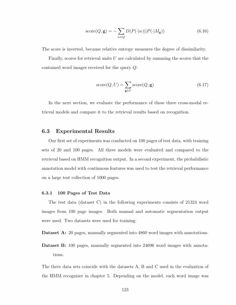
score(Q,g) = −∑w∈Q

D(P (·|w)||P (·|Mg)) (6.16)

The score is inverted, because relative entropy measures the degree of dissimilarity.

Finally, scores for retrieval units U are calculated by summing the scores that the

contained word images received for the query Q:

score(Q,U) =∑g∈U

score(Q,g) (6.17)

In the next section, we evaluate the performance of these three cross-modal re-

trieval models and compare it to the retrieval results based on recognition.

6.3 Experimental Results

Our first set of experiments was conducted on 100 pages of test data, with training

sets of 20 and 100 pages. All three models were evaluated and compared to the

retrieval based on HMM recognition output. In a second experiment, the probabilistic

annotation model with continuous features was used to test the retrieval performance

on a large test collection of 1000 pages.

6.3.1 100 Pages of Test Data

The test data (dataset C) in the following experiments consists of 21324 word

images from 100 page images. Both manual and automatic segmentation output

were used. Two datasets were used for training:

Dataset A: 20 pages, manually segmented into 4860 word images with annotations.

Dataset B: 100 pages, manually segmented into 24696 word images with annota-

tions.

The three data sets coincide with the datasets A, B and C used in the evaluation of

the HMM recognizer in chapter 5. Depending on the model, each word image was

123

represented using either discrete or continuous features. The same 400 queries of

length 1 to 4 (100 of each length) that were used in the evaluation of the recognize-

then-retrieve approach were used to retrieve lines and pages as described in sections

6.2.1 and 6.2.2. Each model has two tuning parameters that were determined empir-

ically on the training set by splitting it into a training and a validation portion of

equal size. Separate parameter settings were determined for data sets A and B.

Tables 6.1 and 6.2 show mean average precision scores obtained from retrieval

with 20 pages of training data. The results were calculated from the actual ranked

lists and lists that have been padded to include all retrieval units in the test set

(see the alternate retrieval evaluation in section 5.2.2). Tables 6.3 and 6.4 show the

same results for 100 pages of training data. Our discussion here is restricted to the

evaluation scores obtained with the padded lists, because they do not depend on the

length of the returned list (which has an effect on mean average precision calculation;

see section 5.2.2).

The test data was structured into pages and lines using the manual segmentation

output. In order to test the impact of the segmentation errors due to automatic

segmentation on retrieval performance, we repeated the page retrieval experiments

on the automatically segmented test set.

The best model appears to be the probabilistic annotation model with continuous-

space features (CPA). In most cases, it outperformed not only the other cross-modal

retrieval models, but also the retrieval approach based on HMM recognition output.

On data set A, the HMM only surpasses the other models for page retrieval using

queries with 3 and 4 words. The DPA model performs best for multi-word queries

on automatic segmentation output. We believe this somewhat mixed picture of per-

formance can be attributed to the tuning parameters, which are not close enough

to their optimal settings. This is due to the small size of the training set A, which

was used to determine the parameters. The larger training set B, which consists of

124

Experiment Query length DPA CPA DCM A/HMMLine 1 word .1052∗ .1385 .0898∗ .0933∗

Retrieval w/ 2 words .2046∗ .2685 .1164∗ .1655∗Manual 3 words .3142 .3357 .1353∗ .2630∗

Segmentation 4 words .3217∗ .3495 .1481∗ .2903∗Page 1 word .2318∗ .2960 .1946∗ .1818∗

Retrieval w/ 2 words .2327∗ .2668 .1766∗ .2451∗Manual 3 words .2175∗ .2769 .2042∗ .2777

Segmentation 4 words .2908∗ .3161∗ .2584∗ .3874

Page 1 word .1841 .2129 .1628∗ n/aRetrieval w/ 2 words .1769 .1660 .1633 n/aAutomatic 3 words .2549 .1724∗ .1763∗ n/a

Segmentation 4 words .2737 .1560∗ .1550∗ n/a

Table 6.1. Mean average precision scores for retrieval experiments on 100 pages oftest data, using 20 pages of training data (data set A). The scores are calculatedfor the ranked lists as they are returned by the retrieval process. Results that aresignificantly different from the best result in each row are marked with an asterisk(∗).

Experiment Query length DPA CPA DCM A/HMMLine 1 word .1070∗ .1392 .0940∗ .0979∗

Retrieval w/ 2 words .2048∗ .2685 .1168∗ .1662∗Manual 3 words .3142 .3357 .1355∗ .2631∗

Segmentation 4 words .3217∗ .3495 .1482∗ .2903∗Page 1 word .2774 .3141 .2526∗ .2740∗

Retrieval w/ 2 words .2358∗ .2672 .1846∗ .2574Manual 3 words .2176∗ .2769 .2067∗ .2811

Segmentation 4 words .2908∗ .3161∗ .2589∗ .3880

Page 1 word .2331 .2371 .2292 n/aRetrieval w/ 2 words .1811 .1667 .1720 n/aAutomatic 3 words .2554 .1724∗ .1801∗ n/a

Segmentation 4 words .2737 .1560∗ .1556∗ n/a

Table 6.2. Mean average precision scores for retrieval experiments on 100 pages oftest data, using 20 pages of training data (data set A). The ranked lists were paddedto full length before the score calculation. Results that are significantly different fromthe best result in each row are marked with an asterisk (∗).

125

Experiment Query length DPA CPA DCM B/HMMLine 1 word .1001∗ .1602 .0995∗ .0826∗

Retrieval w/ 2 words .1716∗ .2843 .0753∗ .1175∗Manual 3 words .2111∗ .2695 .0832∗ .1312∗

Segmentation 4 words .2592∗ .3827 .1313∗ .1394∗Page 1 word .2322∗ .2993 .2129∗ .1623∗

Retrieval w/ 2 words .2147∗ .3272 .1785∗ .1984∗Manual 3 words .2132∗ .2860 .1732∗ .2097∗

Segmentation 4 words .2289∗ .3406 .2232∗ .2200∗Page 1 word .2073∗ .2416 .1653∗ n/a

Retrieval w/ 2 words .1939∗ .2276 .1676∗ n/aAutomatic 3 words .2081 .2438 .1682∗ n/a

Segmentation 4 words .2292∗ .3089 .2271 n/a

Table 6.3. Mean average precision scores for retrieval experiments on 100 pages oftest data, using 100 pages of training data (data set B). The scores are calculatedfor the ranked lists as they are returned by the retrieval process. Results that aresignificantly different from the best result in each row are marked with an asterisk(∗).

Experiment Query length DPA CPA DCM B/HMMLine 1 word .1011∗ .1614 .1043∗ .0878∗

Retrieval w/ 2 words .1717∗ .2843 .0758∗ .1186∗Manual 3 words .2111∗ .2695 .0833∗ .1314∗

Segmentation 4 words .2592∗ .3827 .1314∗ .1395∗Page 1 word .2580∗ .3283 .2701∗ .2629∗

Retrieval w/ 2 words .2148∗ .3281 .1868∗ .2208∗Manual 3 words .2132∗ .2861 .1760∗ .2163∗

Segmentation 4 words .2289∗ .3406 .2236∗ .2228∗Page 1 word .2350∗ .2678 .2284∗ n/a

Retrieval w/ 2 words .1942∗ .2279 .1754∗ n/aAutomatic 3 words .2081 .2438 .1717∗ n/a

Segmentation 4 words .2292∗ .3089 .2279 n/a

Table 6.4. Mean average precision scores for retrieval experiments on 100 pages oftest data, using 100 pages of training data (data set B). The ranked lists were paddedto full length before the score calculation. Results that are significantly different fromthe best result in each row are marked with an asterisk (∗).

126

100 page images, yielded better tuning parameter settings and shows the superior

performance of the CPA model more clearly. It consistently outperforms the other

models in all experiments.

On the large training set (B), the performance of both the discrete models (DPA

and DCM) and the HMM generally tends to be lower. One reason for this is the

increased vocabulary of the training collection. Another is the inability of the dis-

crete models to make fine distinctions between features. The feature discretization

technique lumps together feature values with small differences. However, such fine-

grained information may be useful for distinguishing word classes. The continuous-

space annotation model, which uses kernels for feature comparisons, can make such

distinctions. Another disadvantage of the discrete models is the smoothing of fea-

ture distributions, which does not take into account how the feature tokens were

generated. In particular, an improved smoothing should take into account that the

location of bins carries some information about the contained feature values. This

could be exploited to implement a coarse notion of feature distance, similar to the

kernel density estimate for continuous-space features.

In the majority of the cases, CPA performs substantially better with more training

data than with less. This is particularly true of the document retrieval results on

automatic segmentation output. It appears that the fine-grained modeling of feature

distributions is also of significant benefit in this case. While the performance on

automatic segmentation output is generally lower than on manual segments, it is still

satisfying.

Tables 6.5 and 6.6 show precision scores at the top 5 retrieved items for all ex-

periments. Similarly to the mean average precision scores in Tables 6.1 through 6.4,

CPA only clearly shows its superior performance with 100 pages of training data.

The precision scores decrease with longer queries and tend to be low. This may be

explained by Table 5.3, which shows that the number of relevant items per query de-

127

Experiment Query length DPA CPA DCM A/HMMLine 1 word 0.1680 0.2100 0.1960 0.1680

Retrieval w/ 2 words 0.1080 0.1000 0.0380∗ 0.0660∗Manual 3 words 0.1120 0.1120 0.0520∗ 0.0840

Segmentation 4 words 0.0900 0.1040 0.0600∗ 0.0800∗Page 1 word 0.2940 0.3160 0.2560∗ 0.3060

Retrieval w/ 2 words 0.2000 0.2320 0.1420∗ 0.2120Manual 3 words 0.1340∗ 0.1760 0.1260∗ 0.1900

Segmentation 4 words 0.1320∗ 0.1260∗ 0.1040∗ 0.1620Page 1 word 0.2360 0.2260 0.2280 n/a

Retrieval w/ 2 words 0.1540 0.1160 0.1200 n/aAutomatic 3 words 0.1360 0.1040∗ 0.1320 n/a

Segmentation 4 words 0.1120 0.0620∗ 0.0840∗ n/a

Table 6.5. Precision scores at the top 5 retrieved items using 20 pages of trainingdata. The ranked lists were padded to full length before the score calculation. Resultsthat are significantly different from the best result in each row are marked with anasterisk (∗).

Experiment Query length DPA CPA DCM B/HMMLine 1 word 0.1480∗ 0.2360 0.2040 0.1740∗

Retrieval w/ 2 words 0.0700∗ 0.1180 0.0360∗ 0.0540∗Manual 3 words 0.0720∗ 0.0980 0.0460∗ 0.0560∗

Segmentation 4 words 0.0740∗ 0.1160 0.0380∗ 0.0500∗Page 1 word 0.2500∗ 0.3420 0.2580∗ 0.2940∗

Retrieval w/ 2 words 0.1720∗ 0.2640 0.1520∗ 0.1940∗Manual 3 words 0.1720∗ 0.1900 0.1300∗ 0.1640

Segmentation 4 words 0.1120∗ 0.1380 0.0900∗ 0.1140Page 1 word 0.2620 0.2600 0.2360 n/a

Retrieval w/ 2 words 0.1540 0.1900 0.1620 n/aAutomatic 3 words 0.1380 0.1660 0.1240∗ n/a

Segmentation 4 words 0.1080 0.1120 0.0940 n/a

Table 6.6. Precision scores at the top 5 retrieved items using 100 pages of trainingdata. The ranked lists were padded to full length before the score calculation. Resultsthat are significantly different from the best result in each row are marked with anasterisk (∗).

128

creases with the length of the query. For queries consisting of 4 words, the expected

number of relevant items that fall into the top 5 ranks is 2.03 for page retrieval and

1.18 for line retrieval assuming perfect ranking (all relevant items at the top). This

translates into expected precision scores of .406 for page retrieval and .236 for line

retrieval, again assuming perfect retrieval. Seen from this perspective, the precision

scores of the CPA model are quite good.

6.3.2 1100 Pages of Test Data

The test collection we used in the previous experiments is large in terms of word

images (21324) and space (609MB), but there are only 100 pages. Compared to

collection sizes that are typically used in the information retrieval of text, this is

very small. In order to get an idea of the scalability of our cross-modal retrieval

approach, an evaluation of its performance on larger collection is desirable. Unfor-

tunately, relevance judgments are hard to obtain, even for the limited definition of

relevance judgments that is used here. The relevance judgments are generated from

transcriptions, which need to be mapped to the retrieval units 1-to-1.

Almost 16,000 transcriptions for the roughly 152,000 papers of George Washing-

ton are available at the Library of Congress’ website [110]. On the site, each image

of a page may be linked to 0 or more transcriptions. Many pages contain one or

more letters, which are all transcribed in separate text files. This technique is de-

sirable for the organization of the collection into letters which may extend beyond

page boundaries, but unfortunately not for our purposes. We do not perform any

document layout analysis and do not know the beginning and end of documents,

hence we perform page retrieval. When trying to obtain the transcription of an en-

tire page, several problems may occur. An image may contain multiple letters, but

not all of them may be transcribed, resulting in an incomplete transcription of the

page. Another problem is caused by letters that span multiple pages. This makes it

129

necessary to align portions of the available transcription with each of the pages that

the transcription is linked with, a non-trivial problem in itself [111, 49].

We avoid problems that fall into the latter category by generating a collection

that only consists of page images which link to one transcription. Furthermore, we

do not use images if they are linked to by more than one transcription. Even though

this guarantees a 1-to-1 mapping of transcriptions to page images, there may still be

some smaller problems: For example, the page may still consist of multiple letters, of

which only one is transcribed (yielding an incomplete transcription), and hyphenated

words in the image are typically transcribed as one word (causing tainted relevance

judgments). Given the cost of human annotation, we will use the collection as it is for

automatic relevance judgment generation, and manually inspect some retrieval results

to assess how often relevance has been misjudged. The resulting test set consists of

1100 page images.

The training collection is the same set of 100 pages as used before, and retrieval

is performed on the output of the probabilistic annotation approach with continuous-

space features (CPA), because it resulted in the best performance. We used 39 fea-

tures: 6 scalar features and 33 DFT coefficients (the optimal number that has been

determined in section 3.2.2). The queries are the same as above, but queries with

no relevant items in the test set are removed. There are now 96, 80, 61, and 27

queries with lengths of 1 to 4 words respectively (previously there were 100 queries

per category).

Table 6.7 shows the MAP results obtained on this dataset. The performance has

decreased compared to the results on 100 test pages. Several factors have contributed

to this (see Figure 6.4 for illustrations):

Dataset selection: The dataset has been selected entirely based on whether ground

truth data is available for the pages. As a result, pages were selected from all

portions of the collection, causing a greater variability in writing style and

130

Query length: 1 word 2 words 3 words 4 wordsMAP (short ranked lists): .0765 .0391 .0553 .0841MAP (padded ranked lists): .0994 .0413 .0558 .0842

Table 6.7. Mean average precision scores for retrieval experiments on 1100 pagesof test data, using 100 pages of training data (data set B). The first row shows thescores that were calculated from the (short) ranked lists that were returned by theranking algorithm. The second row shows the scores that were obtained when theranked lists were padded to full length.

(a) Severe image degradation.

(b) Crossing out of words, writing in be-tween lines.

(c) Narrow writing style with no availabletraining data, difficult to segment.

Figure 6.4. Example images from the 1100 pages test set, showing the difficulty ofthis data set.

131

possibly more writers. Our training data was selected from a mostly coherent

portion of the collection, so it may not be adequate to cover all the observed

writing styles.

Image quality: A substantial number of the images are of such poor quality that

they are hard to read. The page images in previous test sets are generally

readable.

Segmentation quality: Due to the decreased image quality, and the fact that the

segmentation algorithm was evaluated on our training sets, a visual inspection

of the segmentation output indicated that the segmentation quality is worse

than on the datasets it has been evaluated on. This affects the retrieval quality.

Partial transcriptions: A visual inspection of the alignment between the available

transcriptions and the word image content in 100 of the 1100 page images

showed that on average about 85% of the word content in a page image is

transcribed (the standard deviation is 20%). Since the relevance judgments are

based on whether the query terms appear in the transcription, it is likely that

some relevant pages have been judged non-relevant, because one or more of the

query terms occurred in the non-transcribed portion of the page. For this reason

we expect the true MAP scores to be slightly higher than the ones in Table 6.7.

We believe it is possible to improve the results in Table 6.7, using linguistic post-

processing and enhanced image processing and document analysis techniques.

6.3.3 10k Pages

We have set up a system that is based on 10,000 test images and 200 pages of

training data. The size of this data set makes it very difficult to obtain page-aligned

ground truth data, which would be necessary for an evaluation of page retrieval

performance. Non-aligned, and potentially partial ground truth data is available for

132

all test pages. However, the ground truth transcriptions are organized into letters

and not pages. When the problem of transcript alignment (for example, see [49] or

[111]) is solved to a satisfactory degree, an evaluation would be possible.

6.4 Learning Behavior

In this section we look at the learning behavior of the cross-modal retrieval ap-

proach, specifically the probabilistic annotation approach with continuous-space fea-

tures (CPA). We conducted experiments with 100 pages of test data and subsets of

varying size from 100 pages of training data to test the influence of more training data

on retrieval performance. Starting with two pages, the training set size is increased

in steps of two pages up to the full size of 100 pages. The test data was structured

into lines and documents for retrieval with the same set of 1 to 4 word queries used

before.

Figure 6.5(a) shows the relation of retrieval performance (measured using mean

average precision) to the number of training pages used. As more training pages

become available the performance improves, because an increasing number of query

words is encountered in the training set. The performance increases sharply for queries

of all lengths at around 35 training pages, indicating that a substantial portion of

the queries has relevant training instances in that portion of the training data. At

around 70% of the training set, the performance levels off. Using more training data

does not further increase mean average precision.

To further investigate what causes the performance increase with larger training

sets, we plotted the training instances for query terms. Figure 6.5(b) shows the

fraction of training instances for query words included in the training set (including

repetitions), Figure 6.5(c) shows the fraction of query terms for which at least one

training instance is available. The latter shows a clear correlation with Figure 6.5(a):

the “hump” in the beginning, the sharp increase around 35 training pages, and the

133

0

0.05

0.1

0.15

0.2

0.25

0.3

0.35

0.4

0 10 20 30 40 50 60 70 80 90 100

Mea

n av

erag

e pr

ecis

ion

Number of training pages

1-word queries2-word queries3-word queries4-word queries

(a) Mean average precision.

0

10

20

30

40

50

60

70

80

90

100

0 10 20 30 40 50 60 70 80 90 100

% T

rain

ing

inst

ance

s co

ntai

ned

Number of training pages

1-word queries2-word queries3-word queries4-word queries

(b) Training instances used.

0

10

20

30

40

50

60

70

80

90

100

0 10 20 30 40 50 60 70 80 90 100

% T

rain

ing

voca

bula

ry c

onta

ined

Number of training pages

1-word queries2-word queries3-word queries4-word queries

(c) Query vocabulary coverage.

5

10

15

20

25

30

35

40

45

50

55

60

0 10 20 30 40 50 60 70 80 90 100

% T

est v

ocab

ular

y co

ntai

ned

Number of training pages

Vocabulary coverage

(d) Test vocabulary coverage.

Figure 6.5. Plots showing the learning behavior of the CPA cross-modal retrievalmodel. Coverage of the vocabulary used in queries and the percentage of the trainingdata used as a function of the number of training pages.

leveling off around 70 pages. While the plots in Figures 6.5(a) and 6.5(b) correlate,

the relationship is not as distinctive. After a certain number of training instances

has been reached, more training data does not seem to improve retrieval performance

any more. An indication for this is that the mean average precision does not increase

beyond 70 training pages, although this portion of the training set contains almost

20% of the total training instances.

134

Figure 6.5(d) shows the coverage of the test vocabulary, which shows the char-

acteristics of Heaps’ law (see section 4.4.1). The maximum vocabulary coverage is

55%, meaning no queries can be constructed for 45% of the words in the test set.

Furthermore, the rate of increase shows that a substantially larger test set vocabu-

lary coverage can only be achieved with much larger training collections. This would

mean increasing the size of the training set beyond that of the test collection, which

is not practical. A practical approach is to use synthetic training data to increase the

vocabulary coverage. In section 6.7 we take a first look at this idea.

6.5 Linguistic Post-Processing of Annotation Results

So far, our annotation models have ignored a word image’s context, that is, the

adjacent word images in the sequence defined by the reading order. That means our

calculation of classification probabilities only uses features that are associated with

the image we would like to annotate.

However, the occurrence of a particular word in a text is typically not independent

of previous words. It has been shown that the quality of handwriting recognizers can

be improved significantly, when the context of a word image in a text is taken into

account [77, 58, 117]. A common way of modeling sequence data where neighboring

samples are constrained with respect to one another is the Hidden Markov Model,

which we have used in chapter 5 to recognize word image sequences.

6.5.1 Constraint Model

Here we use an HMM to model the dependencies between adjacent words in the

image sequence that we annotate probabilistically. The dependencies take the form of

a word bigram model, which constrains the annotations that are chosen for adjacent

word images. This model is a post-processing step, in the sense that the HMM is

135

placed on top of the probabilistic annotation output. The approach described here

only applies to the probabilistic annotation models (CPA and DPA).

Wi−1 Wi Wi+1

Fi+1FiFi−1

Figure 6.6. Graphical representation of a Hidden Markov Model. The Wi are hiddenstate variables, the Fi are observations.

As we have seen in section 5.1.3, HMM-based recognizers typically use the Viterbi

algorithm [25] to determine the most likely state sequence w1, . . . , wN that generated

the observed feature vectors f1, . . . , fN . This is particularly useful when the states

correspond to words in a vocabulary and the resulting state sequence is to be inter-

preted as text (a sentence, paragraph, . . . ). However, we would like to argue here

that another optimality criterion is better suited to retrieval, which is our target ap-

plication. Here the goal is not to create readable text, but to correctly annotate as

many states as possible. Therefore, we would like to maximize the expected number

of correct states. That is, at each point i in a sequence of length N , we are looking

for

wi = argmaxw

P (Wi = w|F1 = f1, . . . , FN = fN) (6.18)

= argmaxw

P (Wi = w,F1 = f1, . . . , FN = fN)

= argmaxw

P (Wi = w, f1, . . . , fi)P (fi+1, . . . , fN |Wi = w, f1, . . . , fi)

= argmaxw

P (Wi = w, f1, . . . , fi)P (fi+1, . . . , fN |Wi = w)

= argmaxw

αi(w) βi(w),

136

where αi(w) and βi(w) can be computed using the forward and backward algorithms

[86], which are dynamic programming techniques similar to the Viterbi algorithm.

For our retrieval application we are not interested in recognition, i.e. determining the

element wi which yielded the maximum probability in equation (6.18). Instead we

will calculate

P (Wi = w|F1 = f1, . . . , FN = fN)

for all w ∈ V. The result is an annotation distribution for the i-th word image

in the sequence, which now takes into account all observations f1, . . . , fN , whereas

the probabilistic annotation based on the original cross-modal model only uses the

observation fi.

What remains is the calculation of the forward and backward probabilities αi(w)

and βi(w). We show the recursive calculation of the forward probability, the backward

algorithm is similar:

αi(w) = P (Wi =w, f1, . . . , fi)

= P (fi|Wi =w, f1, . . . , fi−1)P (Wi =w, f1, . . . , fi−1)

= P (fi|Wi =w)∑w′∈V

P (Wi =w,Wi−1 =w′, f1, . . . , fi−1) (∗)

= P (fi|Wi =w)∑w′∈V

P (Wi =w|Wi−1 =w′, f1, . . . , fi−1)P (Wi−1 =w′, f1, . . . , fi−1)

= P (fi|Wi =w)∑w′∈V

P (Wi =w|Wi−1 =w′)αi−1(w′) (∗)

α1(w) = P (f1|W1 =w)P (W1 =w),

where (∗) indicates that we have used the fact that a random variable is independent

of the ancestors of its parent, given its parent (factoring according to the HMM graph

in Figure 6.6).

Both the forward and backward algorithm require prior probabilities P (W1 =

w), a transition probability table with entries P (Wi = w|Wi−1 = w′) and emission

137

probabilities P (fi|Wi = w). The word priors and transition probabilities may be

estimated from the annotations of the training collection T and other text sources O

as described in section 5.1.2:

P (W1 = w) =1

3

c(w, T )

|T |+

1

3

c(w,O)

|O|+

1

3

1

|V|,

P (Wi = w|Wi−1 = w′) =1

3

c(w′w, T )∑v∈V c(w′v, T )

+1

3

c(w′w,O)∑v∈V c(w′v,O)

+1

3P (W1 = w).

The emission model may be partly determined from the cross-modal annotation prob-

abilities and equation (6.19):

P (fi|Wi = w) =P (Wi = w|fi)P (fi)

P (Wi = w)(6.19)

P (Wi = w|fi) is the output of the probabilistic annotation model, and P (W1 = w)

may be used in place of P (Wi = w).6 Since we are only interested in the relative

probabilities that are determined by the forward and backward algorithms, and not

the actual values, P (fi) may be regarded as a constant that is factored out.

6.5.2 Experimental Results

Our experiments with the linguistic post-processing technique were conducted on

100 pages of test data, using 100 pages of training data (T ), all manually segmented.

The probabilistic annotation model is CPA. The test data was annotated probabilisti-

cally and we performed retrieval of documents and lines, using the same queries as in

previous experiments. Then the annotation output was post-processed page-by-page

with a bigram language model determined from T and the Jefferson collection (O,

200,000 words) that was used previously with our HMM recognizer.

6P (W1 = w) is really a prior that is valid for all positions i in the sequence.

138

MRR before MRR after Improvement # pages improved / worse.5020 .5378 .0358 99/1

Table 6.8. Mean Reciprocal Rank (MRR) performance scores for 100 test pages,shown before and after linguistic post-processing.

The first evaluation looks at the improvement of the per-word-image annotation

distributions with the post-processing. Table 6.8 shows mean reciprocal rank (MRR)

scores before and after the post-processing step. To calculate this score, the annota-

tion distribution of each word image is ordered by decreasing annotation probability.

Then the MRR for a page is the reciprocal rank of the correct annotation term, av-

eraged for all word images of that page. If the correct annotation term is always

assigned the highest probability, the MRR would be 1. When the correct annotation

term tends to occur at lower ranks, MRR approaches zero. If the correct annotation

term is not contained in the annotation distribution, which can happen if the term

is not contained in the annotation vocabulary or if the annotation list is truncated,

we set the reciprocal rank to 0. The results clearly show that the post-processing is

beneficial. Although the improvement in MRR is modest, it is very consistent. The

MRR score improved for 99 out of the 100 test pages. The MRR scores also show that

the probabilistic annotation technique performs well. On average, the correct anno-

tation term appears at rank two in the annotation distribution. This is quite good,

especially when considering that OOV terms have been included in the evaluation.

We now take a look at the impact of linguistic post-processing on retrieval perfor-

mance. Table 6.9 shows the mean average precision scores that were obtained with the

probabilistic annotation output using continuous-space features, before and after the

post-processing step. The retrieval performance has clearly benefitted from applying

word bigram constraints. After post-processing, the precision scores are substantially

higher than before. The difference in mean average precision is even greater than the

139

Experiment Query length Before post-proc. After post-proc.Page 1 word .3277 .3706

Retrieval w/ 2 words .3279 .3757Manual 3 words .2861 .3247

Segmentation 4 words .3406 .4234Line 1 word .1627 .2207

Retrieval w/ 2 words .2843 .3650Manual 3 words .2695 .3441

Segmentation 4 words .3827 .4569

Table 6.9. Mean average precision scores shown for retrieval on probabilistic anno-tation output, shown before and after linguistic post-processing. The annotation wasperformed using continuous-space features.

modest improvement in MRR would lead to think. Since the current text source for

the estimation of word bigram probabilities is quite small, it is possible that with a

larger text source further performance improvements could be made.

6.6 Related Cross-Modal Work

Cross-modal models can be applied for any combination of media, given suitable

content representations. Here we discuss cross-modal models that have been proposed

for other domains and compare our model to them. Initially, cross-media models were

proposed by Jeon et al. [41] and Lavrenko et al. [57] for automatic annotation and

retrieval of individual color photographs. Our work extends them to the retrieval

of images of handwriting, which are organized in arbitrary text units (e.g. lines or

documents). Furthermore, this work shows how a bigram language model may be used

to constrain the annotations of adjacent word images, which substantially improves

retrieval performance.

Feng et al. [24] and Lavrenko et al. [56] proposed cross-media models that extends

Jeon et al.’s work to perform annotation and retrieval of video keyframes and color

photographs. Their models use a multiple-Bernoulli distribution to describe the gen-

140

eration of annotation terms (Jeon et al. used a multinomial), which is better suited for

the annotation of photographs. In a multinomial model, the annotations house and

car would compete for probability mass, causing the available probability mass to be

split if both objects occur together. If only one of them is present, all the probability

mass will be concentrated in the corresponding term. This would rank a photograph

with one object in it higher than one with multiple objects (even if the target object

is present). The multiple-Bernoulli model assigns annotation probabilities that do

not suffer from this problem.

Both Feng et al. and Jeon et al. used color and texture features. In the handwriting

domain, such features are not available, only shape can be used. Furthermore, where

discrete image representations are required, we are using a feature discretization that

allows more fine-grained decisions than previously used techniques. Earlier work

represents entire feature vectors with a single discrete token by clustering feature

representations before the annotation process. We believe this corresponds to making

a classification decision in feature space, that removes details which could aid in

the annotation process. We are adopting a more fine-grained discretization strategy

(see section 3.3) that clusters feature vector entries dimension-by-dimension, leaving

classification decisions up to the cross-modal model.

The annotation vocabulary that was used in previous work is much smaller (e.g. 371

words in [41]) than in our case (up to 4226). In addition, since photograph and video

annotations are inherently ambiguous, the problem of OOV terms is not a major

concern, as long as the annotation vocabulary provides a reasonable coverage of the

content. If no annotation word is available for a particular photograph, one can

always resort to using a more general or generic description of the content. For ex-

ample, person could be used instead of swimmer or water in place of pool. In the

handwriting domain, this is not possible. Each word image has exactly one correct

annotation that cannot be replaced.

141

In the remainder of this chapter we investigate the use of synthetic word images

for replacing or complementing natural training data. Such training data could also

be used in a word spotting or recognition-based approach. However, since the cross-

modal models have shown very good retrieval performance and practicability, we have

chosen to evaluate the synthetic data with this approach.

6.7 Synthetic Training Data

Words as the atomic units of recognition and retrieval are convenient, but there are

also some drawbacks associated with this approach. The two main criticisms are that

it is virtually impossible to obtain training data for all words in the test vocabulary

(cf. Figure 6.5(d)) and even if there is training data, it may not be sufficient to

allow the accurate estimation of the conditional feature distributions. In this section

we investigate to what degree these shortcomings can be addressed by generating

synthetic training data that complements existing natural samples of writing.

There has been very little work in this area for handwriting data. Until recently,

there has been no work on synthetic data for cursive Roman script [12]. In that pre-

sentation, Bunke proposed the generation of artificial training data from templates

and by distorting existing handwritten text. He demonstrated how increasingly real-

istic renderings of word images can be generated by obtaining character N-grams of

increasing length N from existing data and using them to render synthetic words. At

the same conference, Varga and Bunke [114] presented a system for generating syn-

thetic training data using random perturbations of existing natural samples. All of

these experiments were conducted on modern handwriting samples of high scanning

quality. Recently, Howe et al. [35] showed how distortions of historical writing can be

used to improve the recognition accuracy of a holistic recognizer.

Ishidera and Nishiwaki [37] described a top-down word image synthesis approach

which they used for handwriting recognition. Their word generation process uses a

142

probabilistic model which places character templates on a canvas. The style of each

character, as well as position and size of the character are sampled at random, to

imitate the typical handwriting variations.

We pursue two strategies for creating artificial data using a template-based ap-

proach. The first is to use a TrueType font, which is similar in appearance to the

target writing, to generate training instances. The second strategy uses a bitmap

font, which has been obtained from the target writing, to create training data by

pasting together images of individual characters. The following sections describe the

training data generation and the retrieval experiments that were used to assess the

effectiveness of using synthetic data in lieu of natural data.

6.7.1 TrueType Font

The general handwriting style that is typically found in the George Washington

collection is called Copperplate or round hand. This writing, which was used in British

commerce in the 18th century, is typical for the founding fathers [81]. Despite its age,

this style has not dropped out of fashion, and a number of TrueType computer fonts

that mimic it can be found.

TrueType [2] is a format for scalable computer fonts developed by Apple Computer,

Inc.. The shapes of characters are defined by curves, which can be easily scaled to any

desired size without distorting the appearance of the characters. For our experiments,

we chose the fonts CounselorScript, CommScriptTT, and CACChampagne. Figure 6.7

shows some sample renderings with these fonts.

The renderings from TrueType fonts are designed to be clean and uniform, and

thus do not exhibit features that are typical of historical handwriting, such as noise,

loss of contrast and variations of slant and skew as well as the writing speed. In order

to generate training data that is closer in appearance to actual historical handwriting

samples, the black-and-white renderings were randomly distorted in a number of ways.

143

(a) CounselorScript font.

(b) CommScriptTT font.

(c) CACChampagne font.

Figure 6.7. Sample renderings with the 3 TrueType fonts that were used in thegeneration of synthetic training data.

(a) Synthetic. (b) Synthetic. (c) Synthetic. (d) Natural.

(e) Synthetic. (f) Synthetic. (g) Synthetic. (h) Natural.

Figure 6.8. Sample renderings of the words same and Regiment using TrueTypefonts, after adding noise and distortions to simulate historical data. The rightmostimages are natural examples provided for comparison.

First, variations in writing speed are simulated by duplicating, preserving or re-

moving image columns according to statistics that have been gathered from actual

dynamic time warps of matching word images (cf. section 4.2.1). The statistics, which

consist of the relative frequencies of the three moves (duplication, preservation, re-

moval), were collected from dynamic time warps performed in [91]. Then the image

144

is smoothed and binarized using a randomized threshold to create the thinning effect

in historical documents, which frequently breaks up thin strokes. We use a technique

similar to the Threshold defect model described in [4]. In the next step, random

salt and pepper noise is added to a rendered image, which is then smoothed. This

simulates the effect of dirt on a page together with the smoothing effect that is cre-

ated by ink slowly being soaked up by the paper. Then the image is slanted with a

small angle that is selected at random. This is to simulate the mistakes introduced

by the deslanting algorithm. Finally, the word image is cleaned (see section 2.3.2)

to remove variations in the background (paper) intensity, and passed through the

deskewing algorithm. The resulting images are then passed to the feature extraction

routine. Some typical examples of the simulated historical writing samples can be

seen in Figure 6.8.

6.7.2 Bitmap Font

A bitmap font contains an image of each allowed character. This finished rep-

resentation makes it difficult to scale the font without loss of quality, which usually

occurs due to aliasing and other problems. The advantage of such a font is that

renderings can be done very efficiently at the native character size of the font.

The Copperplate fonts in the previous section provide a reasonable approximation

to the writing style used in the George Washington collection. However, with a

bitmap font that was obtained from the collection itself, an even better match is

possible. We collected exemplars of all 52 upper- and lower-case characters (A-Z &

a-z) as well as all ten digits, and combined them in a bitmap font. The character and

digit images were manually cleaned using an image manipulation program, in order

to remove dirt and parts from other characters. Figure 6.9 shows all 62 characters of

the resulting bitmap font. Before synthetic word images can be rendered, the slant

145

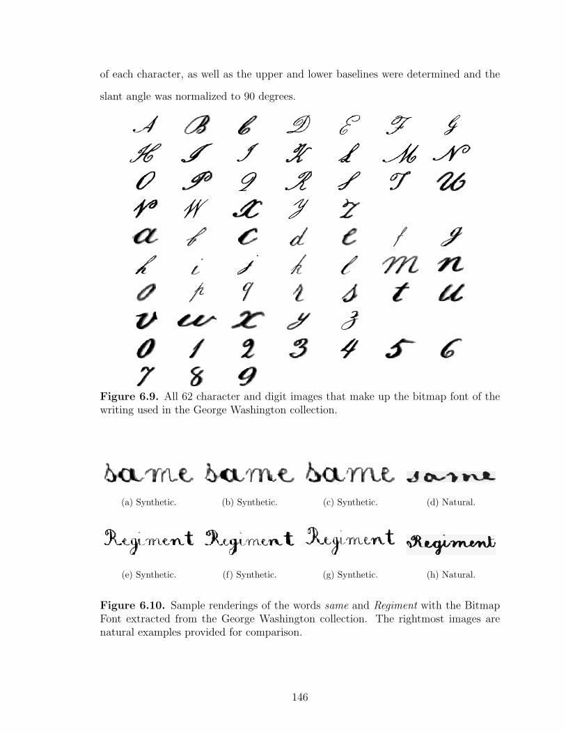
of each character, as well as the upper and lower baselines were determined and the

slant angle was normalized to 90 degrees.

Figure 6.9. All 62 character and digit images that make up the bitmap font of thewriting used in the George Washington collection.

(a) Synthetic. (b) Synthetic. (c) Synthetic. (d) Natural.

(e) Synthetic. (f) Synthetic. (g) Synthetic. (h) Natural.

Figure 6.10. Sample renderings of the words same and Regiment with the BitmapFont extracted from the George Washington collection. The rightmost images arenatural examples provided for comparison.

146

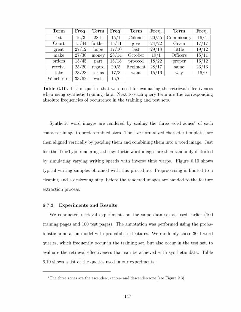
Term Freq. Term Freq. Term Freq. Term Freq.

1st 16/3 28th 15/1 Colonel 20/55 Commissary 16/4Court 15/44 further 15/11 give 24/22 Given 17/17great 27/12 hope 17/10 last 29/18 little 19/12make 27/30 money 28/14 October 19/1 Officers 15/11orders 15/45 part 15/18 proceed 18/22 proper 16/12receive 25/20 regard 20/5 Regiment 28/17 same 23/13take 23/23 terms 17/3 want 15/16 way 16/9

Winchester 33/62 wish 15/6

Table 6.10. List of queries that were used for evaluating the retrieval effectivenesswhen using synthetic training data. Next to each query term are the correspondingabsolute frequencies of occurrence in the training and test sets.

Synthetic word images are rendered by scaling the three word zones7 of each

character image to predetermined sizes. The size-normalized character templates are

then aligned vertically by padding them and combining them into a word image. Just

like the TrueType renderings, the synthetic word images are then randomly distorted

by simulating varying writing speeds with inverse time warps. Figure 6.10 shows

typical writing samples obtained with this procedure. Preprocessing is limited to a

cleaning and a deskewing step, before the rendered images are handed to the feature

extraction process.

6.7.3 Experiments and Results

We conducted retrieval experiments on the same data set as used earlier (100

training pages and 100 test pages). The annotation was performed using the proba-

bilistic annotation model with probabilistic features. We randomly chose 30 1-word

queries, which frequently occur in the training set, but also occur in the test set, to

evaluate the retrieval effectiveness that can be achieved with synthetic data. Table

6.10 shows a list of the queries used in our experiments.

7The three zones are the ascender-, center- and descender-zone (see Figure 2.3).

147

Our experiments include line and word image retrieval. The latter is of particular

interest in this case, because it allows us to to directly assess how well our training

data can mimic actual writing samples. A retrieved word image was only judged

relevant if it had the exact same surface form as the query. That is, the retrieved

word and the query term had to be identical letter-by-letter (in previous experiments

we considered a word relevant if it has the same stem as the query term). The reason

for this is that training data does not have to be generated for every potential surface

form of a term. With this setup, the following experiments were conducted:

Only natural training data: this test run forms the baseline for the subsequent

experiments. Only actual writing samples from the George Washington collec-

tion are used for training.

Only synthetic TrueType data: here we remove all natural training instances for

the query terms in Table 6.10, and replace them with simulated writing samples

that are rendered using the TrueType method. 50 training instances are ren-

dered per query term. The remaining training instances for words that are not

in the query list are kept. This experiment allows us to assess whether retrieval

can be done for queries for which no training data is available. That is, the goal

is to test the suitability of synthetic data for the retrieval of out-of-vocabulary

words.

Only synthetic bitmap font data: the same as above, only that the synthetic im-

ages are rendered using the bitmap font.

Natural and TrueType data: here we add the synthetic TrueType training data

to the natural training instances. This is useful to judge whether a small train-

ing sample for a particular word can be successfully augmented by synthetic

TrueType data. The idea behind this is to increase the robustness of an anno-

148

tation (or recognition) process by providing a larger sample for estimating word

models.

Original and bitmap font data: the same as above, only here the synthetic data

is generated from a bitmap font.

The results of these experiments are shown in Figure 6.11 using recall-precision plots.

0

0.2

0.4

0.6

0.8

1

0 0.2 0.4 0.6 0.8 1

Pre

cisi

on

Recall

Natural writingBitmap font

TrueType fontNatural writing and bitmap font

Natural writing and TrueType font

(a) Line retrieval.

0

0.2

0.4

0.6

0.8

1

0 0.2 0.4 0.6 0.8 1

Pre

cisi

on

Recall

Natural writingBitmap font

TrueType fontNatural writing and bitmap font

Natural writing and TrueType font

(b) Word image retrieval.

Figure 6.11. Recall-precision curves for line and word image retrieval experimentswith synthetic training data. The curves show the performance when using only natu-ral handwriting samples for training, when using only synthetic data (both TrueTypeand Bitmap renderings), as well as when using both synthetic and natural trainingdata together.

Clearly, the retrieval runs with synthetic training data do not perform well. In

the cases where only synthetic training data is used, the performance is the worst,

with the bitmap and TrueType data performing very similarly. When synthetic and

natural data are mixed, the retrieval performance is better, but still substantially

worse than the run which uses only natural training data. The synthetic training

data seems to “pollute” the natural data rather than result in synergetic effects,

causing retrieval performance to decrease.

149

5 10 15 20 250

0.002

0.004

0.006

0.008

0.01

0.012

0.014

0.016

Feature

Mea

n ab

solu

te d

ista

nce

Natural writingBitmap fontTrueType fontRandom

Figure 6.12. Feature-by-feature evaluation of the modeling capabilities of syntheticdata. For each feature, the mean absolute distance of the test feature values to themean of the features values in the model is shown. The shown models are derivedfrom natural handwriting examples (“natural writing” and “random”) and syntheticwriting samples based on the bitmap and TrueType font.

In order to gain some insight into why our synthetic word images could not be used

in place of natural writing samples, we conducted a feature-by-feature evaluation. For

each query word, we extracted all relevant feature vectors from the training set and

the test set. For each feature dimension, we plot the mean absolute distance of the

values in the test set to the mean of the values in the training set, averaged over all

queries. We used the natural writing and the two synthetic data sets as training.

As a baseline, we also plotted a random model. The random model consists of the

natural training instances of a word we selected at random. The random model is

varied every time a different query is evaluated.

The results in Figure 6.12 show clearly that the natural writing yields the smallest

average distance for most feature dimensions. The ranking between the two synthetic

models is not as clear. The bitmap font-rendered samples perform as good or better

than the TrueType-rendered samples for scalar features (features 1 through 6), but

150

the synthetic TrueType samples result in a slightly better model for profile features

(features 7 and up).

It is plausible that the bitmap-rendered samples provide a better match in the

scalar features. These features measure global word similarity, such as the width and

aspect ratio of the bounding box, which can be simulated more effectively with actual

writing samples taken from the dataset that should be modeled. It appears, however,

that the spacing between the character bitmap images is off, causing the TrueType-

rendered samples to be a better model for the profile features. The distance values

that were achieved with the random model show clearly that the modeling of the

synthetic training data needs significant refinement, before the synthetic data can

replace natural writing.

In summary, it must be concluded that natural training data cannot be replaced

with the presented synthetic rendering techniques. No synergetic effects can be ex-

pected when natural writing samples are mixed with synthetic data and the modeling

of out-of-vocabulary terms needs significant improvement in order to be useful. Of

course, this does not mean that creating synthetic training data cannot be done. Our

investigation here should be considered as the first step. Successful simulation of

training data still holds great promise for overcoming the out-of-vocabulary problem.

151

CHAPTER 7

CONCLUSIONS AND FUTURE WORK

In this work, we have presented the first retrieval system for handwritten histor-

ical document images which allows text queries. In building our prototype retrieval

system, we have tackled numerous challenges in a number of areas, including image

processing techniques, feature representations, content annotation techniques and the

design of a user interface (see appendix A). Here we summarize our findings and de-

scribe how the system can be improved to reach the maturity of a commercial grade

system.

7.1 Summary

The development of image processing techniques was based on the observation of

typical properties of historical manuscripts, namely large amounts of noise and hand-

writing variations. By adopting a holistic approach to the analysis of word images

we avoid the word segmentation problem, which is one of the most difficult prob-

lems even when analyzing modern manuscripts with little noise. Using various image

cleaning and normalization techniques, we remove much of the noise and handwriting

variations that complicate the recognition of word images.

Various features were presented for representing word images in historical manu-

scripts. For pair-wise matching of word images with Dynamic Time Warping, we

use profile features, which capture a word’s shape in great detail. For classification

approaches that require vectors of the same dimensionality, we use discrete Fourier

transform descriptors corresponding to low frequencies obtained from the profile fea-

152

tures. Finally, we have shown how to describe multi-dimensional continuous-space

feature vectors in terms of a discrete vocabulary, by discretizing the range of observed

feature values along each feature dimension.

The extracted features were used in the evaluation of three models for the creation

of collection indexes. These are word spotting, recognition followed by retrieval, and

cross-modal retrieval models. In word spotting, word matching is used to create a

partial index for a collection in a semi-automatic way, which requires no training data.

Previous work was only concerned with designing word image matching approaches.

We showed how to carry out the entire word spotting process by investigating clus-

tering algorithms and by demonstrating how cluster candidates for an index can be

selected automatically.

Document recognition is the principal application of handwriting analysis. We

built a Hidden Markov Model recognizer that treats words holistically. The recog-

nition output was used for text retrieval based on the language modeling approach.

This system was used as a baseline for comparison with other retrieval techniques.

The cross-modal retrieval approach uses a model of the joint distribution of word

image features and annotations. These models allow the retrieval in the feature

domain, by mapping query terms to features, and in the annotation domain, by

creating probabilistic annotation vectors for word images. We compared cross-modal

models that use both discrete and continuous-space feature representations with the

retrieval based on HMM recognition output. The best performing model was the

probabilistic annotation model with continuous-space features. We also demonstrated

that performance can be increased even further by applying word bigram constraints

to the probabilistic annotation output.

Using the cross-modal retrieval model approach, we have built a prototype sys-

tem for the retrieval of historical manuscript images from the George Washington

153

collection (http://ciir.cs.umass.edu/demos/). The system allows text queries

and provides a retrieval interface similar to web search engines.

7.2 Future Work

Our prototype system is a proof-of-concept for the feasibility of historical manu-

script image retrieval. Because of the size of this system, which did not allow us

to work out all components to the smallest detail, and the numerous challenges the

problem poses, various limitations remain that need improvement. Here we propose

directions for future work, paying special attention to making our system practicable.

7.2.1 System Improvements

Building an entire retrieval system is a big effort that requires making numerous

decisions. Due to time constraints, some of our choices in this work are not based on

an in-depth investigation of what the optimal alternative would be, but are rather

informed “guesses”. Examples are our particular choice of features and the number

of bins we used to discretize continuous-space features. Since the system performance

depends on such choices, it would be useful to perform a sensitivity analysis to test

the influence of various system parameters on the retrieval performance.

Many of the current system’s shortcomings lie in the document processing step.

The manuscript segmentation algorithm assumes a very simple letter-like layout. In

order to handle a greater variety of layouts, the segmentation must take into account

the possibility of multiple text columns and the presence of images or drawings.

Another shortcoming is that various document image distortions are not taken into

account. This includes simple distortions, such as slightly rotated pages, and the

more complicated distortions that occur when pages are scanned with the binding

still in place.

154

We have experimented with a number of features, but the set we used here should

not be considered ideal. Many features are reported in the literature and we believe

that significant performance increases can be achieved with better features. Our inves-

tigation has focused on holistic word features, but it may be necessary to use features

that take into account local characteristics when making classification decisions.

It is also possible to improve the retrieval models: the cross-modal model in

particular suffers from a problem that is related to the out-of-vocabulary problem.

Some images do not have any word content (e.g. stamps), or contain words that are

illegible (e.g. because they have been crossed out), or they just contain OOV terms.

In those cases the cross-modal model is forced to associate some “random” annotation

words with these images. This could be prevented by allowing the models to reject

images if their features do no resemble any training instance.

Our work here has focused on the papers of George Washington. Many other

collections exist and the techniques presented in this work need to be validated and

refined to allow successful retrieval of a variety of document images. Preliminary

experiments with scanned field notes by Joseph Grinnell1 are promising.

7.2.2 Making the System Practicable

One of the main factors that hamper the quick deployment of this system as a

commercial product is its dependency on author-specific training data. The size of the

George Washington collection, paired with the single-author assumption, has allowed

us to spend a substantial amount of time to acquire training data. Since training

data preparation requires considerably more time per page than human transcription,

automatic document analysis approaches based on author-specific training data are

1Joseph Grinnell (1877-1939) was a professor of zoology at the University of California Berkeleyand the first director of the university’s Museum of Vertebrate Zoology.

155

only feasible for large test collections.2 Currently, it may be more economical to

manually transcribe a smaller collection (up to a few hundred pages) to allow retrieval

using keywords.

So far, our assumption has been that the analyzed document collection has a single

writer (or very few writers). Although we have not investigated the performance of

our system on a collection with many writers, we expect the retrieval performance

to decrease with the current training set, because of the differences in writing style.

This problem could be solved with training data for the relevant writing styles, or

by using representations of word shape that are invariant to changes in writing style.

Because of the large variety of handwriting styles, we expect that the former approach

will provide better performance. A small number of datasets have been used in

the literature, both online (e.g. the UNIPEN database [29]) and offline (e.g. the

IAM data set [75]). They could provide a starting point for more training data,

but unfortunately no historical datasets are available with high-quality ground truth

(except for a set of 20 pages we have made available).

The current approach to training data acquisition is slow. It requires an anno-

tator to transcribe entire pages and then to map the transcriptions to automatic

segmentation output, which itself has to be corrected manually. One way to speed

up this process is to use a transcription mapping approach that automatically deter-

mines correspondences between a transcription and the automatic segmentation of a

document image. Kornfield et al. [49] presented a solution based on a dynamic pro-

gramming algorithm, which can map transcriptions and segmentation output page-

by-page. Rothfeder [97] described another solution for the same problem based on

a Hidden Markov Model. More complicated scenarios still need to be addressed, for

example when transcriptions span multiple physical pages as is the case in the George

2Training data preparation does not only involve the transcription of a document, but also thesegmentation of the document image and the alignment with the transcription (see section 1.5.2).

156

Washington collection. Another idea is to use word spotting to reduce the amount of

human transcription work. Word spotting could be used to cluster a small collection

of unlabeled training images. Once the word images have been grouped, the training

set could be annotated by labeling either some or all clusters. This approach would

greatly reduce the labeling work when compared to a full transcription of the entire

training collection.

Even when training data is available for a collection, it is unlikely that it covers

the entire vocabulary of the test data. Many words such as proper names will be

out-of-vocabulary. We have conducted some preliminary experiments with TrueType

and bitmap font word images in order to create synthetic training data for OOV

terms. The current synthesis models were not able to replace or complement natural

writing samples. More complex models are needed to mimic the variability in human

writing. With a working synthesis model artificial writing samples could be generated

at query time, when the query contains OOV terms.

To a large extent, the problem of OOV terms is due to our holistic approach to

word image analysis. It is unrealistic to expect training collections of a manageable

size to contain all words in the test set. One way around this limitation could be to

analyze word images analytically (bottom-up). Such approaches usually suffer from

very large search spaces, with high computational demands. In order to prune the

search space, a combined analytic and holistic approach could be used.

In the past, retrieval techniques have been mostly concerned with electronic doc-

uments in a symbolic encoding, such as those encountered on the web. Digital li-

braries are a relatively recent phenomenon and require new approaches to retrieval.

This work contributes to this field retrieval techniques for handwritten historical doc-

uments, which form a substantial portion of library collections around the world.

While the present retrieval system can still be improved, we hope to have convinced

157

the reader that this work represents a significant step towards extending retrieval

capabilities to historical manuscripts.

158

APPENDIX A

RETRIEVAL INTERFACE

Most of the popular web search engines follow the same idea when it comes to the

user interface. A text field is used to collect query terms from the user and a ranked list

of documents is returned. In order to help the user decide quickly which documents

are of interest, the title of each document is displayed, together with snippets of text

around occurrences of the query terms in the document. Our demonstration retrieval

system may be accessed at http://ciir.cs.umass.edu/demos/.

The current retrieval interface was developed based on the assumption that the

above interface is widely accepted by users and hence desirable for handwritten docu-

ment retrieval as well. Unfortunately, it is not straightforward to convert web search

engine interfaces to this new domain. The main reason is that there is no ASCII

text representation of a document. The probabilistic nature of the retrieval approach

leaves some uncertainty about word image identities, so it is not entirely clear which

portions of a document are relevant to the query. Additionally, since there is currently

no layout analysis being performed, the annotation information is unstructured. This

makes it impossible to display information such as the title of a document.

Figure A.1 shows the preliminary user interface of the retrieval system with the

top ranks for the query Fort Cumberland. The shown retrieval system performs page

retrieval, so the system returns a ranked list of page images on the left. Since the

images are very big, they are shown at thumbnail size. The thumbnails are intended

to take on the role of the document titles in web search engines, because they allow

the user to get a rough idea of the document content. For example, the user can

159

Figure A.1. Screenshot of the user interface for the retrieval system with results forthe query Fort Cumberland.

decide whether a ranked document contains tabular information or whether it is a

letter.

To the right of the thumbnails, portions of the document that are likely to match

the query terms are displayed. One such “snippet” is created for each query term the

user supplied. Each snippet consists of the word image with the highest annotation

probability for the corresponding query term, plus some additional words (two in the

figure) to the left and right to provide context. Because the snippet selection uses

a probabilistic approach, it is possible that the snippets do not contain the query

terms, but they do appear in the returned page. In such cases it is up to the user to

decide whether to read the page or whether to move on to the next result.

160

At the top of the ranked list, query confidence scores are displayed to provide

feedback about the choice of query terms. Words that occur infrequently in the

training set yield low query confidence scores and tend to give worse results. With the

confidence scores, users can adapt their choice of query terms based on the feedback

they receive. By clicking on a document thumbnail or any of the snippet words, a

full-size version of the page is displayed, with the selected snippet word highlighted.

The ranked list is shown 8 documents at a time, with some page forward/backward

controls at the bottom of the web page (not shown in Figure A.1).

At the moment, the retrieval interface is functional, but there are no browsing

controls for reading through the collection page-by-page. With such functionality and

more advanced browsing capabilities, such as cross-reference following, the current

user interface could be extended to satisfy commercial needs.

161

APPENDIX B

DYNAMIC TIME WARPING LOWER-BOUNDING

In the following we provide some additional information about our proposed lower

bound LB MV for DTW dissimilarity calculations of multivariate time series (see

section 4.3.1).

B.1 Fast kNN Sequential Scanning

In section 4.3.1 we described the seq scan algorithm, which makes use of a lower

bound lb to speed up the search for the nearest neighbor to a query in a data set.

Table B.1 shows the algorithm seq scan knn, which extends seq scan to search for

the set of k nearest neighbors to a given query Q.

B.2 Proof of the Lower-Bound Property

In section 4.3.1.2 we proposed the lower bound LB MV for the DTW dissimilarity

measure for multivariate time series. Here we provide a proof of its lower-bounding

property, which follows the line of thought in Keogh’s work [45].

Proposition: For any two sequences Q and C of the same length n, for any global

constraint on the warping path of the form j − r ≤ i ≤ j + r (i.e. Sakoe-Chiba band

of width r), the following inequality holds: LB MV (Q,C) ≤ DTW (Q,C).

162

seq scan knn(Q, k):N=∅;% initialize set of k nearest neighbors Nfor i = 1 to k

d = f (Q, db entry(i));add (i,d) to N;

end% keep track of maximum distance within Nm = max(i′, d′)∈N (d′);

% scan rest of data base sequentiallyfor i = k+1 to num db entries

l = lb (Q, db entry(i));if l ≥ m

continue; % discarded using lower bound (1)d = f (Q, db entry(i));if d ≥ m

continue; % discarded using f (2)

% db entry(i) is new nearest neighbor, remove maximum (3)% entry in N and add db entry(i)remove

(argmax(i′, d′)∈N(d′)

)from N;

add (i, d) to N;m = max(i′, d′)∈N (d′);

end

% return k nearest neighbors to the queryreturn N;

Table B.1. Fast sequential scanning algorithm for k nearest neighbors search usingthe lower bound lb for f .

Proof: We need to prove

√√√√√√√√√n∑

i=1

d∑p=1

(ci,p − ui,p)2 if ci,p > ui,p

(ci,p − li,p)2 if ci,p < li,p

0 otherwise

≤

√√√√ K∑k=1

d∑p=1

(qik,p − cjk,p)2,

The square root is a monotonic function, so we can remove it:

163

n∑i=1

d∑p=1

(ci,p − ui,p)2 if ci,p > ui,p

(ci,p − li,p)2 if ci,p < li,p

0 otherwise

≤K∑

k=1

d∑p=1

(qik,p − cjk,p)2.

We can prove this inequality by showing that for every summation term on the left-

hand side there exists an equal or greater term on the right-hand side. Since the length

K of the warping path is greater than or equal to n, every term of the summation∑ni=1 . . . on the left-hand side of the above equation can be matched with a greater

or equal term of the summation∑K

k=1 . . . on the right-hand side. Specifically, for a

given index i on the left-hand side, we select (ik, jk) on the right-hand side, such that

i = ik for some jk. A summation term with ik = i is guaranteed to exist because

of the local continuity constraint. Summation terms on the right-hand side are not

matched more than once, since i is different for every matched term on the left-hand

side.

We have left to show

d∑p=1

(ci,p − ui,p)2 if ci,p > ui,p

(ci,p − li,p)2 if ci,p < li,p

0 otherwise

≤d∑

p=1

(ci,p − qjk,p)2,

which we can prove by showing that every summation term on the left is less than or

equal to the corresponding term on the right. We have three cases:

Case ci,p > ui,p:

(ci,p − ui,p)2 ≤ (ci,p − qjk,p)2 (B.1)

We can take the square root of both sides, because the terms in parentheses are

positive: the left-hand side follows from the case (ci,p > ui,p) we are treating.

164

By definition, our global path constraint guarantees jk−r ≤ i ≤ jk +r, from which

we can deduce i − r ≤ jk ≤ i + r. Using the definition of ui,p = max(qi−r,p : qi+r,p),

we get qjk,p ≤ ui,p. Since ui,p < ci,p (definition of case), ci,p − qjk,p is positive.

Hence, we get

ci,p − ui,p ≤ ci,p − qjk,p (B.2)

−ui,p ≤ −qjk,p (B.3)

qjk,p ≤ ui,p (B.4)

which is true.

Case ci,p < li,p:

This proof is straightforward with an argument similar to the above.

Case li,p ≤ ci,p ≤ ui,p:

Trivially we have

0 ≤ (ci,p − qjk,p)2,

where the right-hand side is non-negative. �

165

BIBLIOGRAPHY

[1] Antonacopoulos, A., Gatos, B., and Karatzas, D. ICDAR 2003 page segmen-tation competition. In Proc. of the 7th Int’l Conf. on Document Analysis andRecognition (Edinburgh, Scotland, August 3-6 2003), vol. 2, pp. 688–692.

[2] Apple Computer, Inc. TrueType Reference Manual. Electronically published onthe Internet at http://developer.apple.com/fonts/TTRefMan/, October 1996.

[3] Baeza-Yates, R., and Ribeiro-Neto, B. Modern Information Retrieval. Addison-Wesley, Reading, MA, 1999.

[4] Baird, H. S. Document image defect models. In Structured Document ImageAnalysis, H. S. Baird, H. Bunke, and K. Yamamoto, Eds. Springer-Verlag,Berlin, 1992, pp. 546–556.

[5] Barnard, K., Duygulu, P., de Freitas, N., Forsyth, D., Blei, D., and Jordan,M. I. Matching words and pictures. Journal of Machine Learning Research 3,6 (2003), 1107–1135.

[6] Barnard, K., and Forsyth, D. Learning the semantics of words and pictures.In Proc. of the Int’l Conf. on Computer Vision (Vancouver, Canada, July 9-122001), vol. 2, pp. 408–415.

[7] Belongie, S., Malik, J., and Puzicha, J. Shape matching and object recog-nition using shape contexts. IEEE Trans. on Pattern Analysis and MachineIntelligence 24, 4 (2002), 509–522.

[8] Blei, D. M., and Jordan, M. I. Modeling annotated data. In Proc. of the 26thAnnual Int’l ACM SIGIR Conf. (Toronto, Canada, July 28-August 1 2003),pp. 127–134.

[9] Blei, D. M., Ng, A. Y., and Jordan, M. I. Latent dirichlet allocation. Journalof Machine Learning Research 3 (2003), 993–1022.

[10] Bozinovic, R. M., and Srihari, S. N. Off-line cursive script word recognition.IEEE Trans. on Pattern Analysis and Machine Intelligence 11, 1 (1989), 68–83.

[11] Breuel, T. M. An algorithm for finding maximal whitespace rectangles at ar-bitrary orientations for document layout analysis. In Proc. of the 7th Int’lConf. on Document Analysis and Recognition (Edinburgh, Scotland, August3-6 2003), vol. 1, pp. 66–70.

166

[12] Bunke, H. Recognition of cursive Roman handwriting - past, present and future.Keynote address at the 7th Int’l Conf. on Document Analysis and Recognition,August 3-6 2003.

[13] Cai, D., He, X., Wen, J.-R., and Ma, W.-Y. Block-level link analysis. InProc. of the 27th Annual Int’l ACM SIGIR Conf. (Sheffield, UK, July 25-292004), pp. 440–447.

[14] Cao, H., Ding, X., and Liu, C. Rectifying the bound document image capturedby the camera: A model based approach. In Proc. of the 7th Int’l Conf. onDocument Analysis and Recognition (Edinburgh, Scotland, August 3-6 2003),vol. 1, pp. 71–75.

[15] Cattell, J. M. The time taken up by cerebral operations. Mind 11 (1886),220–242.

[16] Chakrabarti, K., and Mehrotra, S. The hybrid tree: An index structure forhigh-dimensional feature spaces. In Proc. of the Int’l Conf. on Data Engineering(Sydney, Australia, March 23-26 1999), pp. 440–447.

[17] Chen, F. R., and Bloomberg, D. S. Summarization of imaged documents with-out OCR. Computer Vision and Image Understanding 70, 3 (1997), 307–320.

[18] Danielsson, P.-E. Euclidean distance mapping. Computer Graphics and ImageProcessing 14 (1980), 227–248.

[19] Duda, R. O., Hart, P. E., and Stork, D. G. Pattern Classification, 2nd ed.Wiley-Interscience, New York, NY, 2000.

[20] Duygulu, P., Barnard, K., de Freitas, N., and Forsyth, D. Object recognitionas machine translation: Learning a lexicon for a fixed image vocabulary. InProc. of the 7th European Conf. on Computer Vision (Copenhagen, Denmark,May 27-June 2 2002), vol. 4, pp. 97–112.

[21] Edwards, J., Teh, Y. W., Forsyth, D., Bock, R., Maire, M., and Vesom, G.Making latin manuscripts searchable using gHMM’s. In Proc. of the 18th An-nual Conf. on Neural Information Processing Systems (Vancouver, Canada,December 14-16 2004), p. (to appear).

[22] Faloutsos, C. Multimedia IR: Indexing and searching. In Modern InformationRetrieval, R. Baeza-Yates and B. Ribeiro-Neto, Eds. Addison-Wesley, Reading,MA, 1999, pp. 743–747.

[23] Feldbach, M., and Tonnies, K. D. Line detection and segmentation in historicalchurch registers. In Proc. of the 6th Int’l Conf. on Document Analysis andRecognition (Seattle, WA, September 10-13 2001).

167

[24] Feng, S. L., Manmatha, R., and Lavrenko, V. Multiple Bernoulli relevancemodels for image and video annotation. In Proc. of the Conf. on ComputerVision and Pattern Recognition (Washington, DC, June 27-July 2 2004), vol. 2,pp. 1002–1009.

[25] Forney, G. D. The Viterbi algorithm. Proc. of the IEEE 61 (March 1973),268–278.

[26] Freund, J. E. Mathematical Statistics, 5 ed. Prentice Hall, Upper Saddle River,NJ, 1992.

[27] Gorski, N., Anisimov, V., Augustin, E., Baret, O., Price, D., and Simon, J.A2iA check reader: A family of bank check recognition systems. In Proc. ofthe 5th Int’l Conf. on Document Analysis and Recognition (Bangalore, India,September 20-22 1999), vol. 1, pp. 523–526.

[28] Guttman, A. R-trees: A dynamic index structure for spatial searching. InProc. of the ACM SIGMOD Conf. (Boston, MA, June 18-21 1984), pp. 47–57.

[29] Guyon, I., Schomaker, L., Plamondon, R., Liberman, M., and Janet, S.UNIPEN project of on-line data exchange and recognizer benchmarks. InProc. of the Int’l Conf. on Pattern Recognition (Jerusalem, Israel, October9-13 1994), pp. 29–33.

[30] Haralick, R. M. Document image understanding: Geometric and logical layout.In Proc. of the Conf. on Computer Vision and Pattern Recognition (Seattle,WA, June 21-23 1994), pp. 385–390.

[31] Hastie, T., Tibshirani, R., and Friedman, J. The Elements of Statistical Learn-ing: Data Mining, Inference and Prediction. Springer-Verlag, New York, 2001.

[32] Heaps, H. S. Information Retrieval: Computational and Theoretical Aspects.Academic Press, Orlando, FL, 1978.

[33] Herman, S. G. The Naturalist’s Field Journal: A Manual of Instruction Basedon a System Established by Joseph Grinnell. Buteo Books, 1986.

[34] Hofmann, T. Learning and representing topic. a hierarchical mixture model forword occurrences in document databases. In Proc. of the Conf. on AutomatedLearning and Discovery (Pittsburgh, PA, June 11-13 1998).

[35] Howe, N. R., Rath, T. M., and Manmatha, R. Boosted decision trees for wordrecognition in handwritten document retrieval. In Proc. of the 28th Annual Int’lACM SIGIR Conf. (Salvador, Brazil, August 15-19 2005). (to appear).

[36] Hutchison, L. A. D., and Barrett, W. A. Fast registration of tabular documentimages using the fourier-mellin transform. In Proc. of the Int’l Workshop onDocument Image Analysis for Libraries (Palo Alto, CA, January 23-24 2004),pp. 253–267.

168

[37] Ishidera, E., and Nishiwaki, D. A study on top-down word image generationfor handwritten word recognition. In Proc. of the 7th Int’l Conf. on Docu-ment Analysis and Recognition (Edinburgh, Scotland, August 3-6 2003), vol. 2,pp. 1173–1177.

[38] Itakura, F. Minimum prediction residual principle applied to speech recognition.IEEE Trans. on Acoustics, Speech, and Signal Processing 23, 1 (1975), 67–72.

[39] Jain, A. K., and Namboodiri, A. Indexing and retrieval of on-line handwrittendocuments. In Proc. of the 7th Int’l Conf. on Document Analysis and Recogni-tion (Edinburgh, Scotland, August 3-6 2003), vol. 2, pp. 655–659.

[40] Jelinek, F., Bahl, L. R., and Mercer, R. L. Design of a linguistic statisticaldecoder for the recognition of continuous speech. IEEE Trans. on InformationTheory 21 (1975), 250–256.

[41] Jeon, J., Lavrenko, V., and Manmatha, R. Automatic image annotation andretrieval using cross-media relevance models. In Proc. of the 26th Annual Int’lACM SIGIR Conf. (Toronto, Canada, July 28-August 1 2003), pp. 119–126.

[42] Jones, G. J. F., Foote, J. T., Jones, K. Sparck, and Young, S. J. Video mailretrieval: The effect of word spotting accuracy on precision. In Proc. of theInt’l Conf. on Acoustics, Speech and Signal Processing (Detroit, MI, May 8-121995), vol. 1, pp. 309–312.

[43] Kane, S., Lehman, A., and Partridge, E. Indexing george washington’s hand-written manuscripts. Tech. rep., Center for Intelligent Information Retrieval,Univ. of Massachusetts Amherst, 2001.

[44] Kavallieratou, E., Fakotakis, N., and Kokkinakis, G. A slant removal algorithm.Pattern Recognition 33, 7 (2000), 1261–1262.

[45] Keogh, E. Exact indexing of dynamic time warping. In Proc. of the 28th VeryLarge Databases Conf. (Hong Kong, China, August 20-23 2002), pp. 406–417.

[46] Kim, G., Govindaraju, V., and Srihari, S. N. An architecture for handwrittentext recognition systems. Int’l Journal on Document Analysis and Recognition2, 1 (1999), 37–44.

[47] Kim, S. H., Jeong, C. B., Kwag, H. K., and Suen, C. Y. Word segmentationof printed text lines based on gap clustering and special symbol detection. InProc. of the Int’l Conf. on Pattern Recognition (Quebec City, Canada, August11-15 2002), vol. 2, pp. 320–323.

[48] Ko lcz, A., Alspector, J., Augusteijn, M., Carlson, R., and Popescu, G. V. Aline-oriented approach to word spotting in handwritten documents. PatternAnalysis & Applications 3, 2 (2000), 153–168.

169

[49] Kornfield, E. M., Manmatha, R., and Allan, J. Text alignment with handwrittendocuments. In Proc. of the Int’l Workshop on Document Image Analysis forLibraries (Palo Alto, CA, January 23-24 2004), pp. 195–209.

[50] Krovetz, R. Viewing morphology as an inference process. In Proc. of the 16thAnnual Int’l SIGIR Conf. (Pittsburgh, PA, June 27-July 1 1993), pp. 191–202.

[51] Kwok, T., Perrone, M. P., and Russell, G. F. Ink retrieval from handwrittendocuments. In Proc. of the Conf. on Intelligent Data Engineering and Auto-mated Learning (Hong Kong, China, December 13-15 2000), pp. 461–466.

[52] Lagarias, J. C., Reeds, J. A., Wright, M. H., and Wright, P. E. Convergenceproperties of the nelder-mead simplex method in low dimensions. SIAM Journalof Optimization 9, 1 (1998), 112–147.

[53] Lavrenko, V., Choquette, M., and Croft, W. B. Cross-lingual relevance models.In Proc. of the 25th Annual Int’l SIGIR Conf. (Tampere, Finland, August 11-152002), pp. 175–182.

[54] Lavrenko, V., and Croft, W. B. Relevance-based language models. In Proc. ofthe 24th Annual Int’l SIGIR Conf. (New Orleans, LA, September 9-13 2001),pp. 120–127.

[55] Lavrenko, V., and Croft, W. B. Relevance models in information retrieval. InLanguage Modeling for Information Retrieval, W. B. Croft and J. Lafferty, Eds.Kluwer Academic Publishers, Dordrecht, The Netherlands, 2003.

[56] Lavrenko, V., Feng, S. L., and Manmatha, R. Statistical models for automaticvideo annotation and retrieval. In Proc. of the Int’l Conf. on Acoustics, Speechand Signal Processing (Montreal, QC, May 17-21 2004).

[57] Lavrenko, V., Manmatha, R., and Jeon, J. A model for learning the semanticsof pictures. In Proc. of the 16th Annual Conf. on Neural Information ProcessingSystems (Vancouver, Canada, December 9-11 2003). (to appear).

[58] Lavrenko, V., Rath, T. M., and Manmatha, R. Holistic word recognition forhandwritten historical documents. In Proc. of the Int’l Workshop on DocumentImage Analysis for Libraries (Palo Alto, CA, January 23-24 2004), pp. 278–287.

[59] Leedham, G., Varma, S., Patankar, A., and Govindaraju, V. Separating textand background in degraded documents images — a comparison of globalthresholding techniques for multi-stage thresholding. In Proc. of the 8thInt’l Workshop on Frontiers in Handwriting Recognition (Niagara-on-the-Lake,Canada, August 6-8 2002), pp. 244–249.

[60] Lindeberg, T. Scale-Space Theory in Computer Vision. Kluwer Academic Pub-lishers, Dordrecht, Netherlands, 1994.

170

[61] Lopresti, D., and Tomkins, A. On the searchability of electronic ink. In Proc. ofthe 4th Int’l Workshop on Frontiers in Handwriting Recognition (Taipei, Tai-wan, December 7-9 1994), pp. 156–165.

[62] Lu, Y., and Shridhar, M. Character segmentation in handwritten words - anoverview. Pattern Recognition 29, 1 (1996), 77–96.

[63] Luhn, H. P. The automatic creation of literature abstracts. IBM Journal 2(April 1958), 159–165.

[64] Madhvanath, S., and Govindaraju, V. Using holistic features in handwrittenword recognition. In Proc. of the U.S. Postal Service Advanced Technology Conf.(Washington, DC, November 30 - December 2 1992), pp. 183–199.

[65] Madhvanath, S., and Govindaraju, V. The role of holistic paradigms in hand-written word recognition. Trans. on Pattern Analysis and Machine Intelligence23, 2 (2001), 149–164.

[66] Mahadevan, U., and Nagabushnam, R. C. Gap metrics for word separation inhandwritten lines. In Proc. of the 3rd Int’l Conf. on Document Analysis andRecognition (Montreal, Canada, August 14-15 1995), vol. 1, pp. 124–127.

[67] Manmatha, R., and Croft, W. B. Word spotting: Indexing handwrittenmanuscripts. In Intelligent Multimedia Information Retrieval, Mark T. May-bury, Ed. MIT Press, Cambridge, MA, 1997, pp. 43–64.

[68] Manmatha, R., Han, C., and Riseman, E. M. Word spotting: A new approachto indexing handwriting. In Proc. of the Conf. on Computer Vision and PatternRecognition (San Francisco, CA, June 18-20 1996), pp. 631–637.

[69] Manmatha, R., Han, C., Riseman, E. M., and Croft, W. B. Indexing hand-writing using word matching. In Digital Libraries ’96: 1st ACM Int’l Conf. onDigital Libraries (Bethesda, MD, March 20-23 1996), pp. 151–159.

[70] Manmatha, R., and Rothfeder, J. L. A scale space approach for automaticallysegmenting words from historical handwritten documents. IEEE Trans. onPattern Analysis and Machine Intelligence (2005). (to appear).

[71] Manmatha, R., and Srimal, N. Scale space technique for word segmentationin handwritten manuscripts. In Proc. of the Second Int’l Conf. on Scale-SpaceTheories in Computer Vision (Corfu, Greece, September 26-27 1999), pp. 22–33.

[72] Manning, C. D., and Schutze, H. Foundations of Statistical Natural LanguageProcessing. MIT Press, Cambridge, MA, 2001.

[73] Marr, D. Vision. W. H. Freeman and Company, New York, NY, 1982.

171

[74] Marti, U.-V. Offline Erkennung handgeschriebener Texte. Inauguraldisser-tation, Philosophisch-naturwissenschaftliche Fakultat der Universitat Bern,November 1 2000.

[75] Marti, U.-V., and Bunke, H. The iam-database: an English sentence databasefor off-line handwriting recognition. Int’l Journal on Document Analysis andRecognition 5, 1 (2000), 39–46.

[76] Marti, U.-V., and Bunke, H. Text line segmentation and word recognition in asystem for general writer independent handwriting recognition. In Proc. of the6th Int’l Conf. on Document Analysis and Recognition (Seattle, WA, September10-13 2001), pp. 159–163.

[77] Marti, U.-V., and Bunke, H. Using a statistical language model to improve theperformance of an HMM-based cursive handwriting recognition system. Int’lJournal of Pattern Recognition and Artifical Intelligence 15, 1 (2001), 65–90.

[78] Mohanty, N., Rath, T. M., Lee, A., and Manmatha, R. Learning shape forimage classification and retrieval. In Int’l Conf. on Image and Video Retrieval(Singapore, Singapore, July 20-22 2005). (to appear).

[79] Mori, Y., Takahashi, H., and Oka, R. Image-to-word transformation basedon dividing and vector quantizing images with words. In 1st Int’l Workshopon Multimedia Intelligent Storage and Retrieval Management (Orlando, FL,October 30 1999).

[80] Mukherjee, S., Yang, G., Tan, W., and Ramakrishnan, I. V. Automatic dis-covery of semantic structures in HTML documents. In Proc. of the 7th Int’lConf. on Document Analysis and Recognition (Edinburgh, Scotland, August3-6 2003), vol. 1, pp. 245–249.

[81] Nash, R. Handwriting of the founding fathers. Manuscripts 7, 4 (1955), 208–213.

[82] National Institute of Standards and Technology (NIST), and U. S. Departmentof Defense. Text retrieval conference (trec), 1992.

[83] Pacquet, T., and Lecourtier, Y. Recognition of handwritten sentences using arestricted lexicon. Pattern Recognition 26, 3 (1993), 391–407.

[84] Plamondon, R., and Srihari, S. N. On-line and off-line handwriting recogni-tion: A comprehensive survey. IEEE Trans. on Pattern Analysis and MachineIntelligence 22, 1 (2000), 63–84.

[85] Ponte, J., and Croft, W. B. A language modeling approach to informationretrieval. In Proc. of the 21st Annual Int’l ACM SIGIR Conf. (Melbourne,Australia, August 24-28 1998), pp. 275–281.

172

[86] Rabiner, L. R. A tutorial on hidden Markov models and selected applicationsin speech recognition. Proc. of the IEEE 77, 2 (1989), 257–286.

[87] Ratanamahatana, C. A., and Keogh, E. Making time-series classification moreaccurate using learned constraints. In Proc. of the 4th SIAM Int’l Conf. onData Mining (Lake Buena Vista, FL, April 22-24 2004), pp. 11–22.

[88] Rath, T. M., Kane, S., Lehman, A., Partridge, E., and Manmatha, R. Indexingfor a digital library of George Washington’s manuscripts: A study of wordmatching techniques. Tech. rep., Center for Intelligent Information Retrieval,Univ. of Massachusetts Amherst, 2000.

[89] Rath, T. M., and Manmatha, R. Features for word spotting in historicalmanuscripts. In Proc. of the 7th Int’l Conf. on Document Analysis and Recog-nition (Edinburgh, Scotland, August 3-6 2003), vol. 1, pp. 218–222.

[90] Rath, T. M., and Manmatha, R. Lower-bounding of dynamic time warping dis-tances for multivariate time series. Tech. rep., Center for Intelligent InformationRetrieval, Univ. of Massachusetts Amherst, 2003.

[91] Rath, T. M., and Manmatha, R. Word image matching using dynamic timewarping. In Proc. of the Conf. on Computer Vision and Pattern Recognition(Madison, WI, June 18-20 2003), vol. 2, pp. 521–527.

[92] Rath, T. M., Manmatha, R., and Lavrenko, V. A search engine for histori-cal manuscript images. In Proc. of the 27th Annual Int’l ACM SIGIR Conf.(Sheffield, UK, July 25-29 2004), pp. 369–376.

[93] Rath, T. M., Rothfeder, J. L., and Lvin, V. B. The BoxModify tool, 2004.(computer program).

[94] Ratzlaff, E. H. Inter-line distance estimation and text line extraction for uncon-strained online handwriting. In Proc. of the 7th Int’l Workshop on Frontiersin Handwriting Recognition (Amsterdam, The Netherlands, September 11-132000), pp. 33–42.

[95] Ravela, S., and Manmatha, R. Retrieving images by appearance. In Proc. of theInt’l Conf. on Computer Vision (Bombay, India, January 4-7 1998), pp. 608–613.

[96] Reicher, G. M. Perceptual recognition as a function of meaningfulness of stim-ulus material. Journal of Experimental Psychology 81 (1969), 275–280.

[97] Rothfeder, J. L. Aligning transcripts to automatically segmented historicaldocuments. M.S. project report, University of Massachusetts Amherst, 2005.

[98] Rothfeder, J. L., Feng, S., and Rath, T. M. Using corner feature correspon-dences to rank word images by similarity. In Proc. of the Workshop on DocumentImage Analysis and Retrieval (electronically published) (Madison, WI, June 202003).

173

[99] Russell, G., Perrone, M. P., Chee, Y.-M., and Ziq, A. Handwritten documentretrieval. In Proc. of the 8th Int’l Workshop on Frontiers in Handwriting Recog-nition (Niagara-on-the-Lake, Canada, August 6-8 2002), pp. 233–238.

[100] Sakoe, H., and Chiba, S. Dynamic programming algorithm optimization forspoken word recognition. IEEE Trans. on Acoustics, Speech and Signal Pro-cessing 26 (1980), 623–625.

[101] Salton, G., and Buckley, C. The trec eval program, 1991. (contains modifica-tions by other authors).

[102] Sankoff, D., and Kruskal, J. B. Time Warps, String Edits, and Macromolecules:The Theory and Practice of Sequence Comparison. Addison-Wesley, Reading,MA, 1983.

[103] Sayre, K. M. Machine recognition of handwritten words: A project report.Pattern Recognition 5, 3 (1973), 213–228.

[104] Scott, G. L., and Longuet-Higgins, H. C. An algorithm for associating thefeatures of two patterns. Proc. of the Royal Society of London B224 (1991),21–26.

[105] Song, F., and Croft, W. B. A general language model for information retrieval.In Proc. of Int’l Conf. on Information and Knowledge Management (KansasCity, MO, November 2-6 1999), pp. 316–321.

[106] Srihari, S. N., Huang, C., and Srinivasan, H. A search engine for handwrittendocuments. In Document Recognition and Retrieval XII, Proc. of SPIE (SanJose, CA, January 19-20 2005), vol. 5676, pp. 66–75.

[107] Steinherz, T., Rivlin, E., and Intrator, N. Offline cursive script word recognition- a survey. Int’l Journal on Document Analysis and Recognition 2, 2-3 (1999),90–110.

[108] Tan, C. L., Cao, R., and Shen, P. Restoration of archival documents using awavelet technique. IEEE Trans. on Pattern Analysis and Machine Intelligence24, 10 (2002), 1399–1404.

[109] Tan, C. L., Huang, W., Yu, Z., and Xu, Y. Imaged document text retrievalwithout OCR. IEEE Trans. on Pattern Analysis and Machine Intelligence 24,6 (2002), 838–844.

[110] The Library of Congress. George Washington Papers. Electronically publishedat http://memory.loc.gov/ammem/gwhtml/gwhome.html, 2004.

[111] Tomai, C. I., Zhang, B., and Govindaraju, V. Transcript mapping for historichandwritten document images. In Proc. of the 8th Int’l Workshop on Frontiersin Handwriting Recognition (Niagara-on-the-Lake, Canada, August 6-8 2002),pp. 413–418.

174

[112] Triebel, R. Automatische Erkennung von handgeschriebenen Worten mithilfedes Level-building Algorithmus, December 1999. Student Thesis, Institut furInformatik, Albert-Ludwigs-Universitat Freiburg (in German).

[113] Trier, Ø. D., Jain, A. K., and Taxt, T. Feature extraction methods for characterrecognition - a survey. Pattern Recognition 29, 4 (1996), 641–662.

[114] Varga, T., and Bunke, H. Generation of synthetic training data for an HMM-based handwriting recognition system. In Proc. of the 7th Int’l Conf. on Docu-ment Analysis and Recognition (Edinburgh, Scotland, August 3-6 2003), vol. 1,pp. 618–622.

[115] Vinciarelli, A. A survey on off-line cursive word recognition. Pattern Recognition35, 7 (2002), 1433–1446.

[116] Vinciarelli, A. Application of information retrieval techniques to single writerdocuments. Pattern Recognition Letter (2004). (to appear).

[117] Vinciarelli, A., Bengio, S., and Bunke, H. Offline recognition of unconstrainedhandwritten texts using HMMs and statistical language models. IEEE Trans-actions on Pattern Analysis and Machine Intelligence 26, 6 (2004), 709–720.

[118] Vinciarelli, A., and Luettin, J. Off-line cursive script recognition based oncontinuous density HMM. In Proc. of the 7th Int’l Workshop on Frontiersin Handwriting Recognition (Amsterdam, The Netherlands, September 11-132000), pp. 493–498.

[119] Wolf, C., Jolion, J.-M., and Chassaing, F. Text localization, enhancement andbinarization in multimedia documents. In Proc. of the Int’l Conf. on PatternRecognition (Quebec City, Canada, August 11-15 2002), vol. 4, pp. 1037–1040.

[120] Woodworth, R. S. Experimental Psychology. Holt, New York, 1938.

[121] Wu, V., Manmatha, R., and Riseman, E. M. Textfinder: An automatic systemto detect and recognize text in images. IEEE Trans. on Pattern Analysis andMachine Intelligence 21, 11 (1999), 1224–1229.

[122] Yi, B.-K., Jagadish, H. V., and Faloutsos, C. Efficient retrieval of similartime sequences under time warping. In Proc. of the 14th Int’l Conf. on DataEngineering (Orlando, FL, February 23-27 1998), pp. 201–208.

[123] Yosef, I. Bar, Kedem, K., Dinstein, I., Beit-Arie, M., and Engel, E. Classifica-tion of hebrew calligraphic handwriting styles: Preliminary results. In Proc. ofthe Int’l Workshop on Document Image Analysis for Libraries (Palo Alto, CA,January 23-24 2004), pp. 299–305.

[124] Zhai, C. Risk Minimization and Language Modeling in Text Retrieval. PhDthesis, Carnegie Mellon University, Pittsburgh, PA, July 2002.

175

[125] Zheng, Y., Li, H., and Doermann, D. Text identification in noisy documentimages using Markov random field. In Proc. of the 7th Int’l Conf. on Docu-ment Analysis and Recognition (Edinburgh, Scotland, August 3-6 2003), vol. 1,pp. 599–603.

[126] Zhu, Y., and Shasha, D. Warping indexes with envelope transforms for queryby humming. In Proc. of the ACM SIGMOD Conf. (San Diego, CA, June 9-122003), pp. 181–192.

[127] Zipf, G. Human Behaviour and the Principle of Least Effort. Addison-Wesley,Cambridge, MA, 1949.

176