(1) All Bank of England. The views expressed in this paper are those of the authors, and not necessarily those of the Bank of England or its committees. We are grateful to Andrew Bell, Alex Brazier, Paul Brione, Marcus Buckmann, Oliver Bush, Patrick Calver, Shiv Chowla, Sebastian de-Ramon, Stephen Dickinson, Nic Garbarino, Andrew Gracie, Amit Kothiyal, Antoine Lallour, Katie Low, Damien Lynch, Clare Macallan, Alex Michie, Ali Moussavi, Casey Murphy, Tobi Neumann, Simon Pittaway, Amar Radia, Ani Rajan, Katie Rismanchi, Fiona Shaikh and Tamarah Shakir for comments and contributions. Philip Massoud and Karam Shergill provided excellent research assistance. All speeches are available online at www.bankofengland.co.uk/speeches Rethinking Financial Stability Speech given by Andrew G Haldane, Chief Economist, Bank of England Co-authored with David Aikman, Sujit Kapadia and Marc Hinterschweiger (1) ‘Rethinking Macroeconomic Policy IV’ Conference, Washington, D.C. Peterson Institute for International Economics 12 October 2017

Welcome message from author
This document is posted to help you gain knowledge. Please leave a comment to let me know what you think about it! Share it to your friends and learn new things together.
Transcript

(1) All Bank of England. The views expressed in this paper are those of the authors, and not
necessarily those of the Bank of England or its committees. We are grateful to Andrew Bell, Alex Brazier, Paul Brione, Marcus Buckmann, Oliver Bush, Patrick Calver, Shiv Chowla, Sebastian de-Ramon, Stephen Dickinson, Nic Garbarino, Andrew Gracie, Amit Kothiyal, Antoine Lallour, Katie Low, Damien Lynch, Clare Macallan, Alex Michie, Ali Moussavi, Casey Murphy, Tobi Neumann, Simon Pittaway, Amar Radia, Ani Rajan, Katie Rismanchi, Fiona Shaikh and Tamarah Shakir for comments and contributions. Philip Massoud and Karam Shergill provided excellent research assistance.
All speeches are available online at www.bankofengland.co.uk/speeches
1
Rethinking Financial Stability Speech given by
Andrew G Haldane, Chief Economist, Bank of England
Co-authored with David Aikman, Sujit Kapadia and Marc Hinterschweiger(1)
‘Rethinking Macroeconomic Policy IV’ Conference, Washington, D.C.
Peterson Institute for International Economics
12 October 2017

All speeches are available online at www.bankofengland.co.uk/speeches
2
2
Introduction
The theme of this conference is “Rethinking Macroeconomic Policy”. When it comes to financial stability,
that theme could hardly be more appropriate. The global financial crisis has been the prompt for a complete
rethink of financial stability and policies for achieving it. Over the course of the better part of a decade, a
deep and wide-ranging international regulatory reform effort has been underway, as great as any since the
Great Depression.
On cost grounds alone, a systematic rethink and reform of regulatory standards has been fully justified.
While the costs of the global financial crisis are still being counted, it seems likely they will be the largest
since at least the Great Depression. Two approaches are typically used to gauge these costs of crisis:
the cumulative loss of output relative to its trend and the cumulative fiscal costs of supporting the financial
system.1 Let’s take these in turn.
Chart 1 looks at the path of output relative to a simple measure of its pre-crisis trend in the US, UK, France
and Germany after the Great Depression of 1929 and the Great Recession of 2008. In either case, it is
debatable whether estimated “pre-crisis trends” were sustainable, as they may have been artificially inflated
by credit booms. Nonetheless, it is clear that the output losses from both crises, relative to pre-crisis trends,
have been extremely large and long-lasting.
In the US, the level of output is currently around 13% below a continuation of its pre-crisis trend. Ten years
into the Great Depression, output was around 28% below its pre-crisis trend. Even if not quite on the scale
of the 1930s, the global financial crisis has imposed a huge opportunity cost on US citizens. In the UK, the
losses since the Great Recession, currently at around 16% of pre-crisis GDP, are larger than in the US and
indeed larger than those that followed the Great Depression. The crisis opportunity costs for UK and
euro-area citizens have been the highest for at least a century.2
Much the same picture emerges if we look at measures of the fiscal cost of crisis. Again, there are a number
of methods for gauging this cost. But one simple metric is to look at the pattern of government debt-to-GDP
ratios after the Great Depression and Great Recession, recognising that the larger part of the debt
sustainability cost of crisis typically arises from the denominator shrinking than from the numerator rising.
Chart 2 plots these debt-to-GDP ratios, again for the US, UK, France and Germany.
It suggests that, in the decade after the Great Depression, levels of government debt relative to GDP had
increased by around 28 percentage points in the US, 9 percentage points in Germany, but actually declined
in the UK. Since the Great Recession, levels of debt relative to GDP have increased by, on average,
1 For example, Hoggarth, Reis and Saporta (2001).
2 Figures in this paragraph calculate a continuation of pre-crisis GDP using the average growth rate of output in the 10 years preceding
the crisis.

All speeches are available online at www.bankofengland.co.uk/speeches
3
3
28 percentage points for the same set of countries. The fiscal cost of the Great Recession, at least on this
metric, is larger than during the Great Depression.
It is against this backdrop that policymakers internationally have engaged in a deep and wide rethink, rewrite
and reform of the global regulatory rules of the game. Wide, reflecting the multi-faceted nature of the
problems, market failures and market frictions exposed within the financial system during the crisis. Deep,
reflecting the severity of the hit to balance sheets, risk appetite and economic activity that the crisis has
inflicted and continues to inflict.
The next section reviews these regulatory reform efforts and their impact on bank balance sheets and market
metrics of banking risk. With a number of reforms yet to be fully enacted, it is too soon to be reaching
definitive conclusions. Nonetheless, some of the key questions thrown up by these regulatory reforms -
conceptual, empirical and practical - are now reasonably clear. We also have almost a decade’s worth of
additional evidence and research on which to draw when assessing these issues.
The following sections discuss some of those issues, drawing on new research and evidence: the calibration
of regulatory standards, balancing the costs and benefits of tighter regulation; the overall system of financial
regulation, balancing underlaps and overlaps, simplicity and complexity, discretion and rules; the impact of
reforms on incentives in the financial system, in particular incentives to avoid regulation; and the evolving
role of macroprudential regulation in safeguarding stability of the financial system.
The financial system is dynamic and adaptive. So any financial regulatory regime will itself need to be
adaptive if it is to contain risk within this system. In the terms used by Greenwood et al (2017), resilience
needs to be “dynamic”. As past evidence has shown, too rigid a regulatory system will soon become otiose.
And there are already calls, in some quarters and in some countries, for a rethink and rewrite of regulatory
rules on which the ink is barely dry.3 This poses both opportunities and threats.
The opportunities arise from the need to keep the regulatory framework fresh and agile. With the best will in
the world, no one could say with certainty how the far-reaching and interwoven reforms to regulation over the
past decade will precisely land. Judging how the financial system might adapt to future trends in financial
technology is even harder to predict. As new evidence, incentives and innovation arise in the financial
system, the opportunity is created for regulators to learn and adapt the regulatory framework
(Carney, 2017a).
Equally, there are also threats to financial stability from any process of change. History is replete with
examples of regulatory standards being diluted or dismantled in the name of enhancing the dynamism of the
financial system and the economy. To follow this course unthinkingly would risk repeating regulatory
3 For example, Calomiris (2017), Greenwood et al (2017), Duffie (2017).

All speeches are available online at www.bankofengland.co.uk/speeches
4
4
mistakes from the past, recent and distant. Only ten years on from the biggest crisis in several generations,
there are already some eerie echoes of those siren voices. With that in mind, we conclude with some
thoughts on issues which might be fruitful for future research on regulatory policy.
International Regulatory Reform
There are already a number of detailed accounts of the regulatory reforms undertaken by international
policymakers over the past decade (Carney (2017b), Duffie (2017), FSB (2017a), Greenwood et al (2017),
Sarin and Summers (2017), Yellen (2017)). The following is a summarised and simplified account of the
state of play. It partitions reform efforts into their microprudential and macroprudential components,
recognising that the two often overlap and are usually mutually reinforcing in their impact.
We focus here squarely on international banking regulation. We do not cover insurance regulation or
international accounting standards. We do not discuss regulatory reforms undertaken nationally, such as the
“Volcker Rule” in the US (Financial Stability Oversight Council (2011)) and the “Vickers proposals” in the UK
(Independent Commission on Banking (2011)). Nor do we discuss international reforms of market
infrastructure – for example, clearing – and financial market instruments (FSB (2017b)). Finally, we do not
cover changes to banks’ large exposures regime and a range of pay and governance reforms.
Microprudential Reform
Under the umbrella of Basel III, international reform of microprudential regulation has focused on four key
areas: capital, leverage, liquidity and resolution. Taking these in turn:
Reform of risk-based capital standards has focused on increasing the quantity and quality of capital held by
banks against their asset exposures. Minimum regulatory requirements for banks’ “core” (common equity)
capital have been raised from 2% under Basel II to 4.5% under Basel III, even for the smallest banks. And
allowable deductions to core capital have been reduced. On quality of capital, the types of financial
instrument eligible as loss-absorbing capital (including for Tier 1) have been tightened considerably. For
example, certain hybrid capital instruments are no longer eligible, as they were shown during the crisis to be
incapable of absorbing loss in situations of stress (Tucker (2013), Moody’s (2010)).
These reforms to capital standards have, encouragingly, been implemented in full by nearly all countries
internationally (FSB (2017a)). Comparing regulatory capital, pre- and post-reform, is not straightforward.
But taking together changes in both the quantity and quality of capital, it has been estimated that Basel III
raised risk-based capital standards for globally systemic banks by a factor of around ten (Cecchetti (2015)).
One of the new elements of the Basel III package was to supplement risk-weighted capital standards with a
risk-unweighted leverage ratio. Because this measure does not require banks or regulators to form a

All speeches are available online at www.bankofengland.co.uk/speeches
5
5
judgement on the riskiness of banks’ assets, it is in principle simpler, more transparent and less subject to
risk-weight arbitrage (Haldane and Madouros (2012)). Indeed, those were among the reasons a number of
countries, including the US and Canada, had a leverage ratio regime ahead of the crisis.4 The Basel III
leverage ratio, set at a minimum level of 3% Tier 1, is due to be implemented internationally by 2018.
A second new element of the Basel III package was to augment solvency with liquidity-based standards.
Banks’ liquidity has long been a pre-occupation of the Basel Committee (Goodhart (2011)). But it took
wholesale liquidity runs on the world’s largest banks during the crisis to provide the impetus for
internationally-agreed liquidity standards. Under Basel III, these take the form of a liquidity coverage ratio
(LCR), designed to ensure banks have sufficient high-quality liquid assets to meet their 30-day liquidity
needs; and a net stable funding ratio (NSFR), designed to ensure banks’ funding profiles are sustainable.
The LCR has been implemented in full in most countries; the NFSR is due for implementation by 2018.5
During the crisis, a crucial missing ingredient from the financial regulatory architecture was found to be the
ability to wind up financial institutions in an orderly fashion – that is, while minimising disruption to financial
markets and the economy and without exposing tax-payers to risk (FSB (2014)). A number of measures
have been taken or are in progress to fill this gap, including the introduction of more effective national
resolution regimes for financial firms and greater cross-border co-operation and co-ordination when dealing
with international banks in situations of stress (FSB (2017c)).
Another element is to ensure banks have sufficient loss-absorbing liabilities which can be “bailed-in” in the
event of failure, to prevent losses being shouldered by tax-payers. The Financial Stability Board has agreed
standards for such Total Loss-Absorbing Capacity (TLAC) for global systemically-important banks (G-SIBs).
These standards are to be phased-in over coming years, to reach a minimum level of 16% from 2019, and
18% from 2022, of the resolution group’s risk-weighted assets, as well as 6% and 6.75% on a leverage
exposure basis, respectively.
Macroprudential Reform
These new or augmented microprudential standards have been supplemented with a set of new
macroprudential measures. These focus on safeguarding the stability of the financial system as a whole
(Tucker (2009), Bank of England (2009, 2011)). The most significant of these reforms have focused on three
areas: macroprudential capital buffers; stress-testing; and shadow banks.
Historically, capital standards have been static requirements. As part of Basel III, a new time-varying
component of banks’ capital was added – the counter-cyclical capital buffer (CCyB). This recognises that
4 And a number of countries, including the UK, introduced leverage ratio capital requirements in the aftermath of the crisis.
5 For LCR, see BCBS (2013a): http://www.bis.org/publ/bcbs238.pdf; for NSFR, see BCBS (2014b):
http://www.bis.org/bcbs/publ/d295.htm

All speeches are available online at www.bankofengland.co.uk/speeches
6
6
risks to the financial system vary over the credit cycle, typically being highest at its peak and lowest at its
trough. The CCyB aims to counteract somewhat that time-varying risk profile, with additional capital required
during the upswing which can be released during the downswing. There is international reciprocity in the
setting of the CCyB to reduce incentives for cross-border arbitrage (BCBS (2010a)). The framework has
been implemented in most jurisdictions.
Similarly, one of the key lessons of the crisis was that some institutions impose greater degrees of risk on the
system because of their size, complexity or interconnectedness (FSB (2010)). Basel III recognises the need
for these systemically-important firms to carry a structurally higher capital requirement, currently of up to
3.5%, to help mitigate the additional risk they bring to the system. These capital add-ons apply to the 30
designated global systemically-important banks (G-SIBs) and the roughly 160 domestic systemically-
important banks (D-SIBs), to be phased-in between 2016 and 2019.
Stress tests were used by regulators before the crisis to assess whether banks had sufficient capital to
withstand an adverse tail event. But these tests tended to be neither comprehensive nor transparent. In
2009, the US authorities undertook a comprehensive stress test of the major US banks and published the
results. For banks failing the test, regulatory restrictions on their behaviour were imposed. For some people,
this marked the turning point for the US financial system. A comprehensive annual stress-testing exercise is
now undertaken in the US.6 More recently, the US has been joined by the UK and the EU, among others.
7
Finally, one of the striking features of the pre-crisis financial system was the emergence of the so-called
“shadow” banking system. In the US, on some definitions, this grew to exceed in size the conventional
banking system (Pozsar et al (2010)). Since the crisis, reform efforts have focused on two areas. First,
specific reforms have been enacted to sectors which, during the crisis, were found to contain fault-lines - for
example, Money Market Mutual Funds (IOSCO (2012)). Second, a framework has been put in place by the
FSB to define and measure shadow banking entities, to publish data on them to enhance market discipline
and to help authorities identify, and develop policy tools for mitigating, the risks they might pose (FSB
(2013a)). The FSB have recently put forward a package of recommendations to address structural
vulnerabilities from the asset management sector (FSB (2017d)).
Supporting this package of regulatory reforms, micro- and macroprudential, have been initiatives to boost the
quantity and quality of reporting by financial institutions. These should help in pricing institution-specific risk
by financial markets and ratings agencies. Notable initiatives have included: enhanced Pillar 3 disclosures
by banks, covering all aspects of the regulatory reform agenda; and the work of the Enhanced Disclosure
Task Force (EDTF), a private sector group established by the FSB. Over time, this has led to increased
compliance with the EDTF disclosure template (Chart 3).
6 The Comprehensive Capital Analysis and Review or CCAR.
7 Dent and Westwood (2016) includes a comparison of international concurrent stress-testing practices.

All speeches are available online at www.bankofengland.co.uk/speeches
7
7
Balance Sheet Impact
So what has been the impact of these regulatory reform measures on banks’ overall resilience? One simple
set of resilience metrics focusses on bank balance sheet measures of solvency and liquidity. Comparisons
of international banks’ balance sheets are made difficult by changes over time in both the definitions of
variables and the sample of banks. We consider a panel of international banks, designated as either global
systemically-important (G-SIB) by the FSB in 2016, or domestic systemically-important (D-SIB). This gives a
panel of 30 G-SIBs and about 160 D-SIBs.8 For each bank, we consider two solvency-based metrics
(leverage and risk-weighted capital) and two liquidity-based metrics (a simple liquid asset ratio and the ratio
of loans to deposits). These measures do not map precisely to Basel definitions.9
Chart 4 looks at a measure of banks’ Tier 1 risk-weighted capital ratios. For both G-SIBs and D-SIBs in our
sample, these have risen significantly over the past decade, almost doubling from around 7-8% to around
13-14%. A very similar picture emerges for leverage ratios (Chart 5). These have also roughly doubled over
the past decade, from around 3% to around 6%. On these metrics, there has been a material strengthening
in solvency-based standards among systemically-important banks over the past decade. This is also the
case for measures of TLAC (see Chart 6 for a sample of UK banks).
Liquidity metrics show a similar pattern of improvement. For example, liquid asset ratios - high-quality liquid
assets as a fraction of the total balance sheet – have risen from around 6% in 2008 to more than 8% (Chart
7), though the increase is more muted for D-SIBs. Meanwhile, the ratio of loans to deposits (LTD) has also
improved, with lending backed by a larger share of stable sources of funding than before the crisis (Chart 8).
Market-Based Metrics
A second set of metrics of bank solvency and liquidity focus on financial market perceptions of bank risk.
There are a wide variety of potential such metrics, each with their own imperfections, including measures of
default such as CDS spreads, bond yields and ratings; measures of volatility, such as option-implied
volatilities; and measures of profitability, such as price-earnings ratios. These are summarised and
evaluated in Sarin and Summers (2016).
8 These banks have been identified based on publicly available lists of systemically-important firms:
• The Financial Stability Board’s list of G-SIBs as of 21 November 2016. • O-SIIs notified to the European Banking Authority as of 25 April 2016. • US bank holding companies (BHCs) subject to the Federal Reserve’s annual Comprehensive Capital Analysis and Review
(CCAR) as of March 2014. • Banks designated as systemically-important financial groups by the Swiss National Bank. • The four major banks in Australia. • The five largest banks in Canada.
These include bank holding companies as well as their primary operating companies where applicable, as well as foreign subsidiaries that are explicitly designated as systemically-important for a particular country. 9 The data are from the Standard and Poor’s Capital IQ database.

All speeches are available online at www.bankofengland.co.uk/speeches
8
8
Chart 9 plots a measure of default – CDS spreads – for a panel of G-SIBs. It shows a familiar pattern of
pre-crisis under-pricing of risk; a rapid re-pricing of default risk during the crisis; and a subsequent partial
unwind. CDS spreads today sit roughly midway between their pre-crisis and mid-crisis averages.
Bank bond spreads and ratings tell a similar story. Assuming pre-crisis banking risk was materially
under-priced, this evidence is consistent with regulatory reform having boosted the resilience of the global
banking system.
At the same time, measures of bank volatility and profitability have seen fewer signs of recovery. Chart 10
plots a measure of the price-to-book ratio of G-SIBs and D-SIBs. This currently lies well below its historic
average and little different than unity. Put differently, if we used a measure of banks’ capital ratios using the
market rather than the book value of their equity, this would suggest a far smaller degree of improvement in
measured bank solvency and resilience (Chart 11), though the effect is less pronounced for D-SIBs.
Sarin and Summers (2016) reconcile these market movements by appealing to the shifts in the franchise
value of banks. Improved solvency standards have decreased the perceived default risk of banks. But
coincident with lower risk are lower returns to banks’ activities, due to the combined effects of stricter
regulation, misconduct fines, low levels of interest rates and increased competition. This leaves banks a
riskier proposition for equity investors than before the crisis, as the residual claimant on profits. But, by and
large, improved solvency standards have reduced risk among bond-holders and depositors in banks.
“By and large” because, accompanying these changes in banks’ capital standards, has been a move
towards putting losses from default onto bond-holders. This can be seen in the evolution of the implied
“support ratings” given to banks by rating agencies. In 2010, holders of the major UK banks’ debt enjoyed
around 4 notches of implied ratings uplift owing to expectations of government support (Chart 12). By 2016,
that had fallen to less than one notch of support. A similar pattern is evident among other global banks.
Calibrating Regulatory Standards
Is the calibration of these new regulatory standards too tough, too lax or just right? That has been among
the most animated of the regulatory debates over the past decade. One standard for comparison is historical
experience. There has been a significant evolution in the levels of both capital and liquidity ratios of the
major banks over the past century. Chart 13 plots a measure of the leverage ratio for the UK and US
banking systems over a long historical sweep,10
while Chart 14 plots a simple measure of the liquidity ratio
for UK banks over the past half-century (see also Jordà et al (2017)).
Both solvency and liquidity ratios have exhibited a long, downwards drift. Between the end of the
10
Chart 13 is not directly comparable with Chart 5 because it is based on a different definition of leverage and sample of banks.

All speeches are available online at www.bankofengland.co.uk/speeches
9
9
19th century and the troughs prior to the financial crisis, leverage ratios fell by around three quarters in the
US and the UK. Liquid asset ratios among UK banks underwent an even larger fall in less than half the
time. Given the scale of these falls, even with the regulatory reforms of the past decade, levels of capital and
liquidity in the banking system are at levels significantly below those 100 and 50 years ago, respectively.
On the face of it, this gives grounds for questioning whether even these revamped regulatory standards are
sufficient to withstand likely future shocks. We should, however, probably be cautious about jumping too
quickly to that conclusion. Over the past century, there has been significant change in the structure of the
financial system, including in the structure, scale and scope of financial regulation and the safety net. Those
changes could mean that simple, historical comparisons of regulatory standards are misleading.
Admati and Hellwig (2013) provide a comprehensive and lucid account of the case for higher capital
standards. Their argument centres on the fact that the impact of higher capital standards on banks’ overall
cost of capital needs to take account of the lower risk that arises from this shift - the Modigliani-Miller offset
(Modigliani and Miller (1958)). It needs also to distinguish between any private costs to banks from tighter
regulation and the social benefits this confers, with the latter the key public policy yardstick.
When it came to re-calibrating regulatory standards for capital and liquidity after the crisis, international
regulators engaged in a detailed, quantitative exercise which sought to weigh these social costs and benefits
of tighter regulation, drawing on existing empirical evidence. The Long-Term Economic Impact (LEI) study,
published by the Basel Committee in 2010, is a useful starting point for discussion of the appropriate
calibration of regulatory standards (BCBS (2010b)).
The main conclusion from this work was that, under conservative assumptions about likely economic costs,
there were positive economic benefits to society from a sizeable increase in the capital banks were required
to maintain. The study did not settle on an optimal level of bank capital. But the results presented were
consistent with societal benefits peaking at a Tier 1 risk-weighted capital ratio of between 16-19%.11
This is
north of most global banks’ current capital ratios.
The range of published estimates in the LEI study reflected different assumptions about the persistence of
the effects of crises on GDP, an area of particular empirical uncertainty in the academic literature. A
contemporaneous study by Miles et al (2013) concluded that optimal capital requirements were likely to be
higher – perhaps around 20% - if account was taken of the offsetting risk and cost of capital effects of higher
solvency standards (the Modigliani-Miller offset).
It is useful to revisit the calibration in the LEI study in the light of subsequent research. A little notation may
be useful to organise this evidence. Suppose the aim of policy is to keep output in the economy, y, as close
11
These figures are expressed in terms of current definitions of capital and risk-weighted assets. The mapping from the estimates
reported in the LEI report and those above are due to Brooke et al (2015).

All speeches are available online at www.bankofengland.co.uk/speeches
10
10
as possible to its trend growth path, y̅. The objective for the authorities is then to minimise a loss function,
which can be written as:
L = (yt − y̅t)2
Let’s simplify further and assume two factors can cause output to deviate from its trend: first, higher capital
requirements, k, which act to reduce output each period by δ; and second, the occurrence of a financial
crisis which, with probability γ, leads to a discrete drop in output of ∆. That is:
yt = y̅t − δk − γ(k)Δ(k)
This captures the view that higher bank capital could reduce credit supply, and hence economic activity, in
the near term. But by making the financial system more resilient to future shocks, it may also reduce the tail
risk of bad macroeconomic outcomes.
Both probability and severity of crises are influenced negatively by the level of bank capital, with the
relationship likely to be convex (γ′(k) < 0, γ′′(k) > 0, ∆′(k) < 0, ∆′′(k) > 0) – that is to say, one would expect
a one percentage point increase in the capital ratio to have a larger dampening impact on the probability and
severity of crisis when banks are close to their regulatory minima than when capital buffers are plentiful.
In this stylised set-up, the marginal condition that defines optimal bank capital is:
δ = −Δ∂γ
∂k− γ
∂Δ
∂k
Optimal capital is higher the lower is δ, the economic cost of a marginal increase in capital requirements; the
greater are γ and Δ, the likelihood and severity of crises; and the greater are ∂γ
∂k and
∂Δ
∂k, the marginal effects
of capital on the likelihood and severity of crises. So what have we learned over the past decade about the
likely magnitude of these parameters?
The Benefits of Higher Capital Requirements
The assumptions underpinning the marginal benefits of higher capital in the LEI study were as follows:
banking crises occur, on average, once every 20-25 years; the median estimate of the cumulative
discounted costs of a crisis is around 60% of annual pre-crisis GDP; each percentage point increase in the
capital ratio reduces the probability of a banking crisis by a smaller amount, ranging from 1.4% to 1% (for a
capital increase from 10% to 11%) to 0.4% to 0.3% (for a capital increase from 14% to 15%); and, finally,
the level of bank capital has no impact on the severity of crisis.

All speeches are available online at www.bankofengland.co.uk/speeches
11
11
Since the LEI report, a rich seam of the literature has emerged on the determinants of crises and their
severity (∆). Some of the most illuminating pieces of this research have drawn on evidence from a long
historical time-series and across multiple countries (for example, Jordà et al (2013), Taylor (2015)). The key
findings are as follows.
First, credit booms are probably the single most important determinant both of the likelihood of crises and of
economic performance in the recovery after them (Schularick and Taylor (2012), Jordà et al (2013)). A
sustained 1 percentage point increase in the credit-to-GDP ratio raises the probability of crisis from 4% to
around 4.3% per year. It also raises the severity of a crisis, with real GDP per capita almost 1% lower after
five years.12
Colleagues at the Bank of England have considered whether it is the level of credit, or its
growth, prior to a crisis that matters most for subsequent economic performance (Bridges et al (2017)). They
find that credit growth has historically been a significant predictor of crisis severity, whereas the level of
indebtedness appears less important.
Second, not all forms of credit are equal. In the post-WWII era, mortgage credit growth has been the
dominant driver of financial crisis risk. And growth in mortgages, rather than in other forms of credit, is the
key determinant of the drag in the recovery phase from crisis (Jordà et al (2017)). Third, asset prices are
also important with ‘leveraged bubbles’ – synchronised house price and mortgage credit booms - particularly
dangerous (Jordà et al (2015)).
Taken together, this evidence is consistent with the probability (γ) and output costs of credit crises (∆) being
at least as large as assumed in the original LEI study, perhaps larger, given the still-high levels of the
credit-to-GDP ratio in most countries, and the monetary and fiscal space available to the authorities at
present relative to the average of the past – a recent paper by Romer and Romer (2017) presents evidence
that this factor is a significant determinant of crisis severity. The still-accumulating output losses during the
recovery phase from this time’s crisis would also point in this direction (Chart 1).
What role does higher bank capital play in reducing the likelihood of financial crises (∂γ
∂k) or their severity (∂∆
∂k)?
At least for the likelihood of crisis, subsequent evidence has tended to be rather ambiguous. Historical
evidence, using aggregate economy-wide covariates, has reached the perhaps surprising conclusion that
bank capital ratios have virtually no predictive power for the occurrence of financial crises in major advanced
economies (Jordà et al (2017)). That is, ∂γ
∂k is indistinguishable from zero. This result holds both in the full
sample (1870-2013) and in the post-WWII period.
Micro-econometric studies on the link between bank failure and bank capital have found a more tangible
relationship, however. For example, Vazquez and Federico (2015) find that US and EU banks with stronger
12
This echoes and extends findings from earlier research by Borio and Lowe (2002), Borio and Lowe (2004) and Drehmann, Borio and
Tsatsaronis (2011), which found credit gap measures to be key determinants of crisis risk.

All speeches are available online at www.bankofengland.co.uk/speeches
12
12
pre-crisis capital and structural liquidity positions were less likely to fail. Berger and Bouwman (2013) report
a similar finding using a longer-run data set of US banks. And a recent study by IMF economists finds that
risk-based capital ratios in the range 15-23% would have been sufficient to absorb losses in the vast majority
of past advanced economy banking crises (Dagher et al (2016)).13
At the time of the Basel Committee’s study, there was little evidence on the impact of bank capital on the
severity of crises (∂∆
∂k), which is why this channel was ignored in the quantitative calibration. That has since
changed. Jordà et al (2017) find that, while bank capital does not prevent a crisis from occurring, it matters
for the pain suffered in its aftermath. They find that real GDP per head is 5 per cent higher 5 years after the
onset of a crisis-related recession if bank capital is above its historical average when the crisis hits.
The benefits of capital in reducing the severity of crisis are also borne out by experience since the crisis.
Chart 15 plots international banks’ capital ratios prior to the crisis against their subsequent lending growth.
The relationship has a statistically significant upward slope. Banks that entered the crisis with higher capital
have, on average, been better able to continue their lending. On average, each extra 1 percentage point of
pre-crisis capital boosted banks’ cumulative lending over the subsequent decade by over 20%.
This finding is corroborated by micro-econometric evidence. Carlson et al (2013) find that US banks with
higher pre-crisis capital ratios had stronger loan growth in its aftermath, with the effect particularly
pronounced at lower capital ratios. Cornett et al (2011) and Kapan and Minoiu (2013) report that banks
relying more heavily on stable sources of funding, such as core deposits and equity capital, continued to lend
relative to other banks during the crisis. And Jimenez et al (2014) find that, in periods of economic
weakness, loan applications were less likely to be rejected by Spanish banks that were well-capitalised.
A recent paper by Bank of England colleagues identifies a distinct channel through which bank capital affects
crisis severity (Tracey, Schnittker and Sowerbutts (2017)). They use banks’ misconduct fines as a novel
instrument to identify exogenous negative bank capital shocks. They find that banks respond to such shocks
by relaxing their lending standards, as measured by the loan-to-value and loan-to-income ratios on new
mortgages. This is likely to increase their vulnerability to future shocks, increasing crisis severity.
This evidence suggests that some of the benefits of higher capital requirements may have been understated
in the original LEI study, with implications for the range of optimal capital requirements. For example, if we
assumed that every percentage point of extra capital increased the level of real GDP each period in the
13
Relatedly, Demirguc-Kunt et al (2010) and Beltratti and Stulz (2012) find that poorly capitalised banks had lower stock returns during
the financial crisis. And Boyson et al (2014) find that banks that entered the recent financial crisis with higher capital were less likely to see their funding dry up during the crisis.

All speeches are available online at www.bankofengland.co.uk/speeches
13
13
aftermath of a crisis by 0.1% – broadly consistent with the evidence here - this would raise optimal capital
requirement by around 2 percentage points, other things equal.14
Working in the opposite direction, however, have been developments in resolution arrangements and new
standards for TLAC. No account was taken of these in the LEI study. But if TLAC can be credibly bailed-in,
including for systemically-important institutions, this would tend to reduce both the likelihood and severity of
future crises.15
It may also discipline banks’ management, avoiding them taking excessive risks in the first
place. Some studies suggest this market discipline effect could be material, reducing the likelihood of a
financial crisis by as much as 30% (Afonso et al (2015), Brandao-Marques et al (2013)).
Colleagues at the Bank of England (Brooke et al (2015)) have estimated that, if these measures of the
beneficial incentive effects of TLAC and credible resolution regimes are correct, and if increased resolvability
in addition reduces the cost of crises by around 60%,16
then optimal capital ratios for the UK banking system
could be up to 5 percentage points lower than would otherwise be the case.
A recent study by economists at the Federal Reserve Board (Firestone et al (2017)) also considers the
impact of improved resolution arrangements. They use estimates from Homar and van Wijnbergen (2016) to
model a reduction in the expected duration of crises from such arrangements. Overall, they find that optimal
capital levels for the US banking system can range from 13% to 25%.
The Costs of Higher Capital Requirements
The costs of higher bank capital requirements arise from potentially tighter credit supply conditions. Banks
may adjust to the need to fund themselves with more equity by tightening lending rates and restricting loan
volumes. The LEI study assumed that each percentage point increase in the capital ratio would raise loan
spreads by around 13 basis points. That translated into a fall in GDP of around 0.1% relative to trend.17
What have we learned about these costs since the LEI study? Cecchetti (2014) documents how banks have
adjusted their balance sheets and credit provision since the introduction of Basel III. He finds that banks
increased their capital ratios significantly, by over 4 percentage points on average, across his sample. Net
interest margins and profitability fell. But with the exception of European banks, banks’ assets increased,
their lending spreads narrowed, lending standards eased, and the ratio of bank credit-to-GDP went up.
14
This calculation is based on the marginal condition for optimal capital reported earlier. We parameterise the crisis probability and
severity functions as follows: 𝛾 = exp (𝛽0 + 𝛽1𝑘) (1 + exp (𝛽0 + 𝛽1𝑘))⁄ ; ∆= 𝜃0 + 𝜃1𝑘. The model is calibrated to deliver an optimal capital
ratio of around 18% when 𝜃1 = 0, i.e. the LEI case. We achieve this by setting 𝛿 = 0.1, 𝛽0 = 0.5, 𝛽1 = −0.2, and 𝜃0 = 10, that is to say, a crisis reduces the level of GDP by 10% relative to baseline. If instead we set 𝜃1 = −0.1, such that each percentage point increase in capital reduced the GDP hit in a crisis by 0.1%, the optimal capital ratio increases to over 20%. 15
See Cunliffe (2017) and Bank of England (2017) for discussion of resolution. 16
This estimate is based on the difference in the estimated cost of crises across their sample depending on whether they occurred
under more or less credible resolution regimes. 17
Admati and Hellwig (2013) have forcefully questioned the basis for assuming such costs, given that standard finance theory would
predict that the cost of debt and equity funding for a bank will decline in response to an increase in its capital position.

All speeches are available online at www.bankofengland.co.uk/speeches
14
14
A recent paper from the BIS (Gambacorta and Shin (2016)) reaches a similar conclusion. It finds that banks
with higher unweighted capital ratios have tended to have higher loan growth, with each one percentage
point increase being associated with higher subsequent lending growth of 0.6 percentage points per year.
This evidence is consistent with the macroeconomic costs of higher bank capital being lower than assumed
in the Basel LEI study. Indeed, taken at face value, it would suggest there have been virtually no costs of
achieving higher levels of capital across the global banking system, at least among most global banks.
While credit conditions have clearly improved since the crisis, it is possible that the recovery in lending might
have been stronger still had capital requirements risen by less. To begin to analyse that question, Chart 16
compares the change in bank capital since Basel III was introduced with subsequent lending growth among
a panel of large international banks. On average, lending growth has been positive over this period,
consistent with Cecchetti (2014).
But credit growth has also tended to be statistically significantly lower among banks that have seen the
largest increase in their capital ratios. On average, banks that have increased their capital ratios by an extra
one percentage point have provided 4% less in cumulative credit since Basel III was introduced (3.5% less if
we exclude European banks). This is very similar to the estimates used by the FSB’s Macroeconomic
Assessment Group (2010), which reported a range of estimates from -0.7% to -3.6%.
There are of course different possible interpretations of this negative relationship. Banks facing weak
macroeconomic conditions may simply have seen a reduction in loan demand and responded by maintaining
higher capital buffers on a voluntary basis. To parse these conflicting interpretations, we turn to recent
econometric evidence on the impact of higher capital requirements.
Aiyar et al (2014, 2016) find that shifts in required capital had large negative effects on UK banks’ lending
decisions. De-Ramon et al (2016) report a similar finding, noting that this has, if anything, increased since
the crisis. Bahaj et al (2016) find that, in times of credit expansion, higher required capital has only a minimal
effect on lending. But when credit growth is weak, higher required capital can result in a large reduction in
lending. This echoes previous research which has found that banks reduce lending in response to negative
capital shocks (Peek and Rosengren (1995)).
Lower lending was one cost of higher equity considered in the LEI study. A second potential cost, not
considered by the LEI study, was the potential for falls in market liquidity in core financial markets - for
example, securities financing markets such as repo. This could potentially raise the cost of capital for users
of these markets. Market commentary in recent years has often laid the blame at the leverage ratio. This, it
is argued, has led some dealer-banks to reduce their inventory holdings and market-making capacity,
thereby reducing secondary market liquidity in some markets.

All speeches are available online at www.bankofengland.co.uk/speeches
15
15
There are of course a variety of other reasons why banks’ willingness to make markets, and why market
liquidity more generally, might have been affected by the crisis – for example, reduced risk appetite and
increased counterparty risk. Moreover, it was plausibly the case that pre-crisis liquidity may have been too
plentiful and too cheap in some financial markets, so some correction in the quantity and pricing of liquidity
was to be expected, and indeed was potentially desirable, from a welfare perspective.
Research at the Bank of England has sought to identify the impact of leverage ratio requirements on the
functioning of UK government bond (‘gilt’) and gilt repo markets, using transaction-level data (Bicu et al
(forthcoming)).18
It does find some causal impact of the leverage requirement on various metrics of liquidity,
a worsening that is particularly acute at quarter-ends. Significantly, the banks most constrained by the
leverage ratio reduced their activity in financial markets most.
At the same time, however, dealers unaffected by the leverage ratio requirement also reduced their liquidity
provision and, if anything, by more. This suggests factors other than the leverage ratio may have been at
work in curtailing liquidity in these markets. It also leaves open the question of whether the correction in
liquidity, even if privately costly, came at any social cost. Baranova, Liu and Shakir (2017) assess the costs
that could arise from regulation which affects market liquidity at different levels of stress. They find higher
costs in benign conditions, but substantial benefits in situations of stress as dealers make markets for longer.
Overall Implications for Optimal Capital
How do these research findings tilt the optimal bank capital calculus relative to the LEI study? Table 1
summarises the evidence. They are a mixed bag. On the benefits side, there is now stronger evidence on
the costs of credit booms and the role of capital in constraining the severity of the downturn in the aftermath
of these booms. It also suggests that the costs of raising extra capital are no larger, and may well be
smaller, than originally anticipated. This strengthens the hand of macroprudential authorities when tightening
capital requirements during a credit boom. Other things equal, it would also increase quantitative estimates
of banks’ optimal capital ratio.
On the other side of the ledger, the LEI study did not anticipate two factors. First, the role of TLAC in
augmenting banks’ capital base in situations of stress, potentially reducing the probability and severity of
crises. Second, higher capital requirements could impose liquidity-related costs on the financial system,
though their scale (and whether they are a social cost) remains open for debate. These arguments, in
particular around resolution, have been used by policymakers in some countries, including the UK, when
coming the view that capital requirements should be lower than in the original LEI study. For example,
having assessed all the factors and evidence within Table 1, the Bank of England’s Financial Policy
Committee judged that the appropriate structural level of Tier 1 equity in the system would be 13 ½% of
18
See the Financial Policy Committee’s June 2016 Financial Stability Report (pp 27-33) for an assessment of market liquidity in UK
markets more broadly. The Securities and Exchange Commission’s Report to Congress contains a detailed assessment of the impact of Basel III and the Volcker Rule on liquidity in US Treasury and corporate debt markets (SEC (2017)).

All speeches are available online at www.bankofengland.co.uk/speeches
16
16
risk-weighted assets (Bank of England (2015c)).
Table 1: Overall Implications of Research Findings for Optimal Capital
Impact on optimal capital:
Benefits:
Likelihood and severity of crises
Impact of capital on probability of crises
Impact of capital on severity of crises
Impact of TLAC and resolution regimes on prob. and severity of crises
Costs:
Impact of capital on credit conditions and growth
Impact of capital on market liquidity (leverage ratio) in normal
conditions
The System of Financial Regulation
Regulatory reform has tended to progress crisis by crisis, market failure by market failure, regulatory
standard by regulatory standard. This is not especially surprising, given the nature of the policy design
process. Nonetheless, if we put together the various pieces of recent regulatory reform, we find a
fundamentally different regulatory jigsaw, or system of financial regulation, than in the past.
One important dimension of that new architecture is the significantly larger number of regulatory rules or
constraints that now operate. On top of risk-based capital standards have been added regulatory rules for
liquidity, leverage and loss-absorbing capital. In other words, we have moved from a system of largely
uni-polar regulation to multi-polar regulation (Haldane (2015)). Some individual parts of the regulatory
rulebook - such as the use of internal ratings-based risk weights - also remain complex.
The new regulatory architecture has also introduced measures which are likely to make for a greater degree
of regulatory discretion. The authorities in the US, UK and euro area have moved to annual stress-testing
exercises in which the stress scenario, modelling framework, success criteria and regulatory response are
each subject to significant degrees of regulatory discretion. Regulators internationally are also now setting a
CCyB requirement, which is also set in a largely discretionary fashion.

All speeches are available online at www.bankofengland.co.uk/speeches
17
17
In short, the new regulatory framework involves a larger number of regulatory constraints, many of which are
individually complex, operating with a greater degree of regulatory discretion than in the past. Some have
questioned whether this system may be too complex (for example, Admati and Hellwig (2011)).
And some of the recent debate on regulatory reform in the US also raises those same concerns (US
Department of the Treasury (2017)).
There are several different dimensions to regulatory complexity. Much has already been written on the
complexity of individual rules or regulatory constraints and the associated potential for regulatory arbitrage
(Haldane and Madouros (2012), Aikman et al (2014), Behn, Haselmann, and Vig (2016)). The Basel
Committee’s Task Force on Simplicity and Transparency are looking into these questions at a practical level.
We do not explore those issues further here.
Instead, we focus on two other dimensions of the system of financial regulation: (i) the number of regulatory
constraints; and (ii) the extent of discretion around each individual regulatory rule.
(i) The Number of Regulatory Constraints
Although the post-crisis architecture places many regulatory constraints on banks, the key going-concern
constraints are risk-weighted capital requirements (RWCR), the leverage ratio (LR), the liquidity coverage
ratio (LCR) and the net stable funding ratio (NSFR). We assess these four constraints, recognising that
other aspects of the regulatory system might also impose binding constraints on banks. For example, stress
testing can be interpreted as holding banks to a different RWCR standard and a potentially different overall
capital calibration (Greenwood et al (2017)).
Some have recently contended that this multi-constraint system of financial regulation might be
over-identified, with potentially distortionary implications for banks’ business models and behaviour. For
example, Greenwood et al (2017) argue that it may be distortionary and unnecessary to have multiple,
independent constraints on banks’ behaviour. And Cecchetti and Kashyap (2016) suggest that the LCR and
NSFR are strongly overlapping in their impact, so that both may not be needed.
These are well-reasoned critiques of the new regulatory framework whose messages should be analysed
carefully when evaluating the new framework. They are just the sort of academic challenge to regulatory
orthodoxy which was so missing in the pre-crisis period. Nonetheless, it is also worth reminding ourselves
why and how such a multiple-constraint framework was arrived at in the first place. At a conceptual level,
three arguments could be used to justify such a multi-pronged approach.
First, banks are subject to multiple sources of risk or balance sheet fault-line. Historical experience suggests
they fail for a variety of different reasons. To misquote Tolstoy, while sound banks tend all to be alike,
unsound banks tend to be unsound in their own way. At least in principle, this could point to the need for

All speeches are available online at www.bankofengland.co.uk/speeches
18
18
different types of regulatory constraint to counter different balance sheet fault-lines: one instrument for each
market failure. This is, if you like, the Tinbergen Rule as it applies to financial regulation (Tinbergen (1952)).
Second, uncertainty as well as risk is pervasive in the financial system. These Knightian (1921) uncertainties
have multiple sources - measurement of the risks banks face, how contagion propagates across the financial
system and how regulatory actions affects behaviour, to name but three. A portfolio of regulatory tools can
be seen as a means of offering insurance against these uncertainties. This is, if you like, the Brainard Rule
as it applies to financial regulation (Brainard (1967)).
Third, any individual regulatory constraint creates incentives for banks to respond in ways which may seek to
avoid or arbitrage the rules. In the next section, we discuss how having multiple regulatory constraints might
mitigate this risk. In this section, we discuss the conceptual case for multiple regulatory constraints before
presenting some new empirical evidence. Table 2 summarises some of the key arguments.
Table 2: Assessment of the relative suitability of Basel III standards to address selected forms of risk
Risk First Best Mitigant Second Best Mitigant Less effective Mitigants
Microprudential solvency risk – ‘true’ asset risk
RWCR: Requires loss absorbing capital to cover solvency risks. If risk can be measured and risk weights can be chosen appropriately, this allows for the greatest level of granularity.
LR: Provides loss absorbing capacity but does not include any risk granularity by design.
LCR & NSFR: Neither ratio attempts to mitigate the risk of losses.
Microprudential solvency risk – ‘unknown’ asset risk under Knightian uncertainty
LR: Effective when risks are unknowable and cannot pinpoint particular asset classes of concern, especially in the face of limited historical data or fat-tailed loss distributions.
RWCR: Provides loss absorbing capacity but may perform less well out-of-sample and vulnerable to model risk (IRB approach) or miscalibration of risk weights (standardised approach).
LCR & NSFR: Neither ratio attempts to mitigate the risk of losses.
Vulnerability to risk shifting arbitrage
RWCR: High degree of granularity reduces the scope for risk-shifting
LCR & NSFR: standardised assumptions mitigate some scope to shift risk but also allow some scope for distortion if weights are miscalibrated.
LR: Greatest scope for distortion through risk shifting because of lack of risk sensitivity.
Vulnerability to gaming
LR: Lack of granularity and degrees of freedom minimises gaming opportunities.
LCR and NSFR: Small number of modelled assumptions offer some safeguard against gaming.
RWCR: High degree of freedom offered to banks increases incentives for gaming, especially under IRB approach.

All speeches are available online at www.bankofengland.co.uk/speeches
19
19
Risk First Best Mitigant Second Best Mitigant Less effective Mitigants
Rapid and unsustainable balance sheet expansion
LR: Requires banks to raise capital to support credit creation, regardless of asset composition.
NSFR: Limits reliance on short and medium-term wholesale funding to support balance sheet expansion.
RWCR: Susceptible to expansion into assets with low measured risk. Places no constraint on debt funding. LCR: 30 day time horizon only limits the expansion funded by very short term liabilities.
Sudden withdrawal of funding due to firm-specific or short-lived market-wide loss of credibility
LCR: Assures available buffer of liquid assets to meet immediate outflows enabling survival of first stages of run/preparation for resolution if appropriate.
NSFR: Reduces runnable fraction of liabilities, thus decreases ex-ante risk of being exposed to a run, but does not directly ensure bank has a buffer of usable short-term liquidity.
RWCR & LR: Higher capital should in principle help banks retain funding, but does not provide a cushion if a run occurs.
Sustained loss of funding due to market-wide liquidity stress leading to slow-burn insolvency
NSFR: Matches liquidity of assets against stability of liabilities to ensure bank is broadly resilient to a medium-term funding run.
LCR: Assures available buffer of liquid assets to meet immediate outflows, but not that maturity transformation is sustainable beyond 30 day horizon.
RWCR & LR: Require small fraction of liabilities to be non-runnable equity but a small amount relative to illiquid assets.
Crystallisation of systemic liquidity risk leading to a fire sales, liquidity hoarding, and/or a contraction in lending
NSFR: Reduces banks’ vulnerability to medium-term liquidity risks and hence the probability of them being required to deleverage rapidly in periods of stress to shore up their liquidity position.
LCR: Reduces reliance on the most unstable short-dated liabilities. Risk that banks liquidating buffers to meet outflows in a stress could exacerbate a fire sale.
RWCR & LR: Do not directly mitigate the likelihood of deleveraging due to liquidity problems.
Capital and Leverage
The objective of the capital framework is to ensure banks have sufficient capital to absorb unexpected losses
and continue lending in situations of stress. RWCRs oblige banks to assign granular risk weights to their
assets. If true risk of an asset can be estimated accurately – it is a “known known” - then the RWCR is
typically better suited than the LR to guarding against solvency risk (Gordy (2003)). Greenwood et al (2017)
conclude “the social optimum can be implemented with a single requirement that each bank maintain a
sufficient ratio of equity to risk-weighted assets, provided the risk weights are chosen appropriately”.
The last part of this sentence is, however, an important proviso. One key question is whether risks in the
financial system are likely to be known with sufficient certainty that they can be estimated meaningfully and
accurately. Based on historical experience, that assumption cannot be taken for granted when it comes to
estimating financial risks. As discussed by Aikman et al (2014), there are at least three reasons for this.

All speeches are available online at www.bankofengland.co.uk/speeches
20
20
First, assigning probabilities is particularly difficult with rare, high-impact events, such as financial crises or
the failure of a large financial institution. Degrees of freedom are small in number, historical precedents
rarely exact and causal mechanisms imperfectly understood. This means estimated default probabilities,
and losses given default, are often highly imprecise. Indeed, that is (one reason) why model-based
estimates of the same underlying risks can differ so significantly across banks (BCBS (2014a)).
Second, the behaviour of complex, interconnected financial systems can be very sensitive to small changes
in initial conditions and shocks. That might be because these systems exhibit multiple equilibria, with
path-dependency or hysteresis. Or it may reflect network feedback effects propagating financial contagion.
Complex systems exhibit tipping points, with small changes in parameter values capable of moving the
system from stability to collapse (Anderson and May (1992), Gai and Kapadia (2010), Gai, Haldane and
Kapadia (2011)). In complex webs, the failure of two identical-looking banks can have very different
implications for financial system stability. The radical uncertainty in such complex webs generates emergent
behaviour which can be near-impossible to predict, model and estimate (Haldane (2016)).
Third, because they contain human actors whose beliefs about the future shape their behaviour today,
financial systems are particularly prone to instabilities and sunspots. If financial market participants are
driven by crowd psychology, emotion and narratives, as much as by economic fundamentals and rational
calculation, then risks are unlikely to be well captured by standard models (Tuckett and Taffler (2008),
Tuckett (2011), Shiller (2017), Bailey et al (2016)). These risks are likely to be highly non-linear, heavily
state and time-dependent and thus significantly fat-tailed.
In a world of such Knightian uncertainty, it may be difficult to estimate risk weights on individual assets with
any degree of precision. Indeed, attempts to do so may result in “over-fitting”, increasing the potential
fragility of these model estimates out-of-sample. In uncertain settings, simpler weighting schemes have
been found, in a variety of different environments, to offer a better defence against “unknown unknowns”
(Gigerenzer (2014)). For example, a 1/N or unweighted asset allocation heuristic (Benartzi and Thaler
(2001)), which allocates an equal amount of wealth to each of the assets in one’s portfolio, has been found
to outperform more complex strategies such as Markowitz’s (1952) mean-variance optimisation in
out-of-sample tests, unless the sample size is very large.19
That logic is one rationale for the use - and, in
some settings, predictive superiority – of the LR in capturing solvency risks. It is a variation of the Brainard
(1967) portfolio argument.
In this vein, Aikman et al (2014) conduct simulations which demonstrate how simple methods, akin to a
leverage ratio, can sometimes dominate complex, risk-weighted approaches to calculating banks’ capital
requirements when guarding against solvency problems out of sample. This is more likely when the
underlying risks are themselves fat-tailed. While complex approaches can appear to perform better
19
For example, DeMiguel et al (2007) find that, for a sample threshold of N = 25, complex rules outperform simple ones only for sample
sizes of in excess of 3000 months (250 years) of data.

All speeches are available online at www.bankofengland.co.uk/speeches
21
21
in-sample, simpler approaches may be more robust to out-of-sample structural shifts and fat tails, the like of
which we have seen in past financial crises, from railways in the 19th century to subprime mortgages in the
21st. This problem is not unique to banks. Stress tests can reduce reliance on banks’ own models. But they
then still rely on regulators’ risk models, which may be vulnerable to similar issues, especially if they are
formulated in an excessively granular manner (Hale et al (2015)).
Liquidity and Funding
Historically, most banks failures are precipitated by insufficient liquidity. Due to maturity transformation,
banks are vulnerable to a sudden withdrawal of funding due to bank-specific or market-wide losses of
credibility. In such circumstances, banks will be more robust if they have a buffer of high-quality liquid assets
allowing them to meet outflows, survive the first stages of a bank run and, if necessary, giving the authorities
time to prepare for resolution. The Basel III LCR was designed and calibrated with these considerations in
mind.
But excessive maturity transformation can also create risks over longer horizons. This highlights the
importance of funding metrics which consider the overall extent to which illiquid assets are supported by
unstable sources of funding. If banks are running a high degree of structural maturity transformation, this
increases the risk of failure. While one could envisage a range of possible structural funding metrics,
including a loan-to-deposit ratio, the Basel III NSFR is designed with these risks in mind.
The NSFR speaks directly to a market failure that arises from a market-wide loss of wholesale funding, the
like of which was exhibited during the crisis. In this way, it may potentially reduce the probability of
damaging asset fire-sales, liquidity hoarding and contractions in lending which may otherwise result. The
NSFR is also likely to complement the leverage ratio in acting as a brake on too-rapid balance sheet
expansion. The leverage ratio ensures that any such expansion is supported by higher capital. The NSFR
ensures any such expansion is supported by more stable funding sources.
None of this is to suggest that these risks could not be met with a different, and perhaps smaller, set of
regulatory constraints. Cecchetti and Kashyap (2016) have recently argued that the LCR or NSFR may be
redundant as one of the constraints is always slack in their simplified bank balance sheet model. Put
differently, the existing system of financial regulation may be over-identified. On the other hand, the horizon
for assessing banks’ liquidity risk may matter. In particular, the LCR and NSFR may complement each other
to the extent there are differences in asset liquidity and funding stability at different maturities and that these
differences evolve over the cycle.

All speeches are available online at www.bankofengland.co.uk/speeches
22
22
An Empirical Assessment of Regulatory Metrics
There are conceptual reasons why a portfolio approach to regulatory design, with a small, complementary
set of constraints, may have merit in a robust control sense: addressing the different risks facing financial
institutions and providing insurance against various uncertainties. Ultimately, however, the extent of
over-identification, and any costs it might impose, will depend on the empirical distribution of shocks to banks
and the state of their balance sheets at the time. To that we now turn, based on crisis experience.
Any counter-factual empirical exercise is subject to huge caveats. Nonetheless, it is revealing to consider
experience during the crisis to see what this revealed about the risks banks faced and how different
regulatory constraints might have handled them. For example, recent research has found the leverage ratio
and structural funding metrics performed well in predicting bank failure during the crisis (Huang and
Ratnovski (2009), Demirguc-Kunt et al (2010), Bologna (2011), Arjani and Paulin (2013), Vazquez and
Federico (2015)). And Lallour and Mio (2016) find that the NSFR had significant discriminatory power in
identifying failing banks during the crisis, after controlling for banks’ solvency ratios.
This line of research typically deploys regression approaches which weight together the information across
different indicators. Here we adopt a somewhat different approach. Specifically, we consider how effective
various combinations of regulatory constraints would have had been in identifying banks which subsequently
failed during the crisis (the “hit rate”), while at the same time avoiding incorrectly signalling stress among
banks which survived (the “false alarm rate”).
To do this, we exploit a dataset on the pre-crisis balance sheet characteristics of global banks developed by
Aikman et al (2014). The dataset includes almost all global banks which had more than $100 billion in
assets at end-2006 – 116 banks in total across 25 countries. A range of balance sheet metrics are proxied
at consolidated (group) level for each of these banks at end-2006. Restricting attention to those banks for
which data are available to compute all of risk-weighted capital ratios, leverage ratios and NSFRs reduces
the sample to 76 banks. If we focus on risk-weighted capital ratios, leverage ratios and loan-to-deposit (LTD)
ratios (as a simplified proxy for the NSFR which captures the ratio of retail loans to retail deposits) the
sample size is 96 banks.20
These banks can be divided into those that ‘survived’ and those that ‘failed’ between 2007 and the end of
2009. The definition and classification of failure follows Laeven and Valencia (2010), supplemented by
additional judgement in a few instances.21
To fix ideas, suppose that banks are subject to a single regulatory
20
The dataset also includes a liquid asset ratio but this is a relatively poor proxy for the liquidity coverage ratio (LCR), so we exclude
consideration of the LCR from this analysis. 21
Because very few banks technically defaulted during the crisis, but many would have without significant government intervention, the
definition of failure is necessarily somewhat judgemental. Beyond clear-cut cases of default or nationalisation, Laeven and Valencia (2010) define banks to have failed if at least three of the following six conditions were present: (i) extensive liquidity support (5 percent of deposits and liabilities to non-residents); (ii) bank restructuring costs (at least 3 percent of GDP); (iii) partial bank nationalisation (eg government recapitalisation); (iv) significant guarantees put in place; (v) significant asset purchases (at least 5 percent of GDP); (vi)

All speeches are available online at www.bankofengland.co.uk/speeches
23
23
metric – the leverage ratio. And using this metric, suppose that we set a cut-off threshold consistent with a
particular calibration of that regulatory standard – a leverage ratio of 3%.
One can identify banks which operated below that standard at a point in time. We define the ‘hit rate’ as the
number of banks which had a leverage ratio below 3% at the end of 2006 and subsequently failed during the
crisis, relative to the total number of banks that failed. And we define the ‘false alarm rate’ as the number of
banks with a leverage ratio below 3% which survived, relative to the total number of banks that survived. If a
3% leverage ratio could perfectly discriminate, its hit rate would be 100% and false alarm rate 0%.
Now suppose that we have flexibility over the cut-off threshold necessary to achieve a particular hit rate, x.
At the same time, we wish to minimise false alarms. As the leverage ratio cut-off increases, the hit rate and
false alarm rate must both go up. The key question is by how much each goes up – the relative balance of
marginal benefits and marginal costs of hits and false alarms – as the leverage ratio cut-off increases.
Charts 17 and 18 plot this for the 76-bank sample. Chart 17 plots the settings of the leverage ratio needed
to achieve particular target hit rates. Chart 18, meanwhile, plots what is referred to as the ‘receiver operating
characteristic’ (ROC) curve. Using the sequence of cut-off thresholds for the leverage ratio from Chart 17,
this plots the sequence of associated hit rates and corresponding false alarm rates at different settings of the
leverage ratio, alongside the 45 degree line which corresponds to the performance of a completely
uninformative metric.
Two points are clear from these charts. First, it is possible to achieve relatively high hit rates of up to 70% at
relatively modest calibrations of the leverage ratio of under 4% and with relatively low false alarm rates of
around 30%. This suggests that, with the benefit of hindsight and abstracting from definitional changes
which affect the interpretation of specific numbers, a leverage ratio of around 4% before the crisis would not
have been met by around 70% of banks which subsequently ended up failing. It served as a decent signal of
subsequent failure.
Clearly, such banks might still have failed during the crisis even with a leverage ratio of above 4%. But the
low false alarm rate at that calibration, corresponding to the observation that most banks which survived the
crisis had a leverage ratio of above 4% going into it, indicates that such a constraint may have helped to
curtail their risk-taking, as measured by their leverage ratio, and reduced their likelihood of failure.
Second, to achieve high hit rates of above 80%, both the calibration of the leverage ratio and the false alarm
rate increase sharply. Achieving a 90% hit rate with a leverage ratio alone requires its calibration to be
boosted to around 5.7%. Even then, it comes at the cost of a high false alarm rate of over 80%. In other
words, the balance of marginal benefits to costs becomes notably less positive when using a singular
deposit freezes and bank holidays. Aikman et al (2014) discuss where the classification of failure departs from Laeven and Valencia (2010).

All speeches are available online at www.bankofengland.co.uk/speeches
24
24
instrument if policymakers have a low tolerance for failure. That matters if, for example, the costs of higher
capital requirements increase non-linearly (Greenwood et al (2017)).
These points are also evident if we assess individually the performance of the RWCR and NSFR. Chart 18
and Table 3 below show that hit rates of 80 or 90% can only be achieved with high false alarm rates and
stringent calibrations of these metrics. Overall, each metric individually does somewhat worse than the
leverage ratio in balancing hit and false alarm rates. And similar results hold when the loan to deposit (LTD)
ratio is considered instead of the NSFR in the wider sample (Chart 19).
Table 3: Target hit rate, calibration of individual regulatory tools and resulting false alarm rate
Target Hit
Rate (%)
LR
Calibration
False Alarm
Rate for LR
Calibration (%)
RWCR
Calibration
False Alarm Rate
for RWCR
Calibration (%)
NSFR
Calibration
False Alarm Rate
for NSFR
Calibration (%)
70 3.82 29.3 8.61 58.5 0.99 70.7
75 4.14 39.0 8.66 58.5 1.05 82.9
80 4.15 39.0 8.71 61.0 1.06 82.9
85 5.00 75.6 9.04 68.3 1.12 87.8
90 5.66 82.9 9.83 73.2 1.17 87.8
Now suppose that the regulator can draw on more than one regulatory metric – for example, a LR, RWCR
and NFSR. This now requires the setting of three cut-off thresholds and so gives more degrees of freedom.
But the objective otherwise remains the same, namely achieving a particular hit rate for signalling bank
failures while minimising false alarms. Chart 18 and Table 4 show the results from these multi-constraint
simulations.
Table 4: Target hit rate, calibration of individual and combined regulatory tools and resulting false
alarm rate
Target Hit
Rate (%) LR Calibration
RWCR
Calibration
NSFR
Calibration
False Alarm Rate for
Combined Regulation (%)
70 3.82 5.52 0.63 29.3
75 3.80 5.52 0.72 36.6
80 4.15 5.52 0.63 39.0
85 3.71 5.52 0.83 51.2
90 4.07 5.53 0.83 53.7

All speeches are available online at www.bankofengland.co.uk/speeches
25
25
At a target hit rate of 70%, a portfolio of regulatory measures does little better than the leverage ratio on its
own in signalling bank stress. At targeted hit rates of over 80%, however, that picture changes. The ROC
curve for the regulatory portfolio lies to the left of all those corresponding to individual metrics. In other
words, it is possible to achieve lower false alarm rates, for the same hit rate, when multiple regulatory metrics
are used. The calibration of each metric in the portfolio is also less stringent than the calibration for each
metric individually.
These results hold when comparing any pair of regulatory metrics with individual metrics – a higher hit rate
per false alarm rate, with less stringent calibrations. It also holds even more strongly in the wider 96-bank
sample when the LTD ratio is considered instead of the NSFR (Chart 19). This suggests that, at least in this
sample, imposing a small number of regulatory constraints can achieve the same hit rate as any singular
constraint, but at a materially lower societal and regulatory cost, as measured by levels of capital and
liquidity and/or regulatory false alarms.
Intuitively, these results broadly accord with the conceptual discussion. A regulatory portfolio can help when
insuring against multiple sources of risk and myriad sources of uncertainty. It also accords with what we
know from various individual case studies of bank failure during the global financial crisis: some banks failed
because they were over-leveraged, others because their assets were excessively risky, others still because
they undertook too much maturity transformation.
Because these fault-lines were, for some banks, reasonably well-correlated – their risk management was
poor across all dimensions – individual regulatory metrics performed fairly well in identifying these banks
prior to them failing. But some banks’ risk-management failings were singular, not plural. Their risk
blind-spots were idiosyncratic and uncorrelated. By using a portfolio of regulatory stress metrics, it is
possible to isolate those banks which were risk-management outliers in one, but not all, dimensions.
Consider two very different banks which failed during the global financial crisis. American bank Countrywide
had a leverage ratio of 7.7% and a risk-weighted capital ratio of 11.6% at the end of 2006. Even if capital
regulation had been much tougher in 2006, it may not have been required to raise capital. But its NSFR was
just 0.76, indicative of the structural liquidity risk it was undertaking. By including the NSFR in the suite of
regulatory metrics, it would have been possible to capture the risks that Countrywide was undertaking
without resorting to materially more stringent capital regulation.
By contrast, Belgian bank KBC Group had an NSFR of 1.12, above the current indicative regulatory
standard. For that time, it also had a reasonable risk-weighted capital ratio of 8.7%, well above the median
capital ratio in the sample. But its leverage ratio was 3.5%. A system of regulation excluding the leverage
ratio would have been unable to capture risks of the type KBC Group was undertaking prior to the crisis.
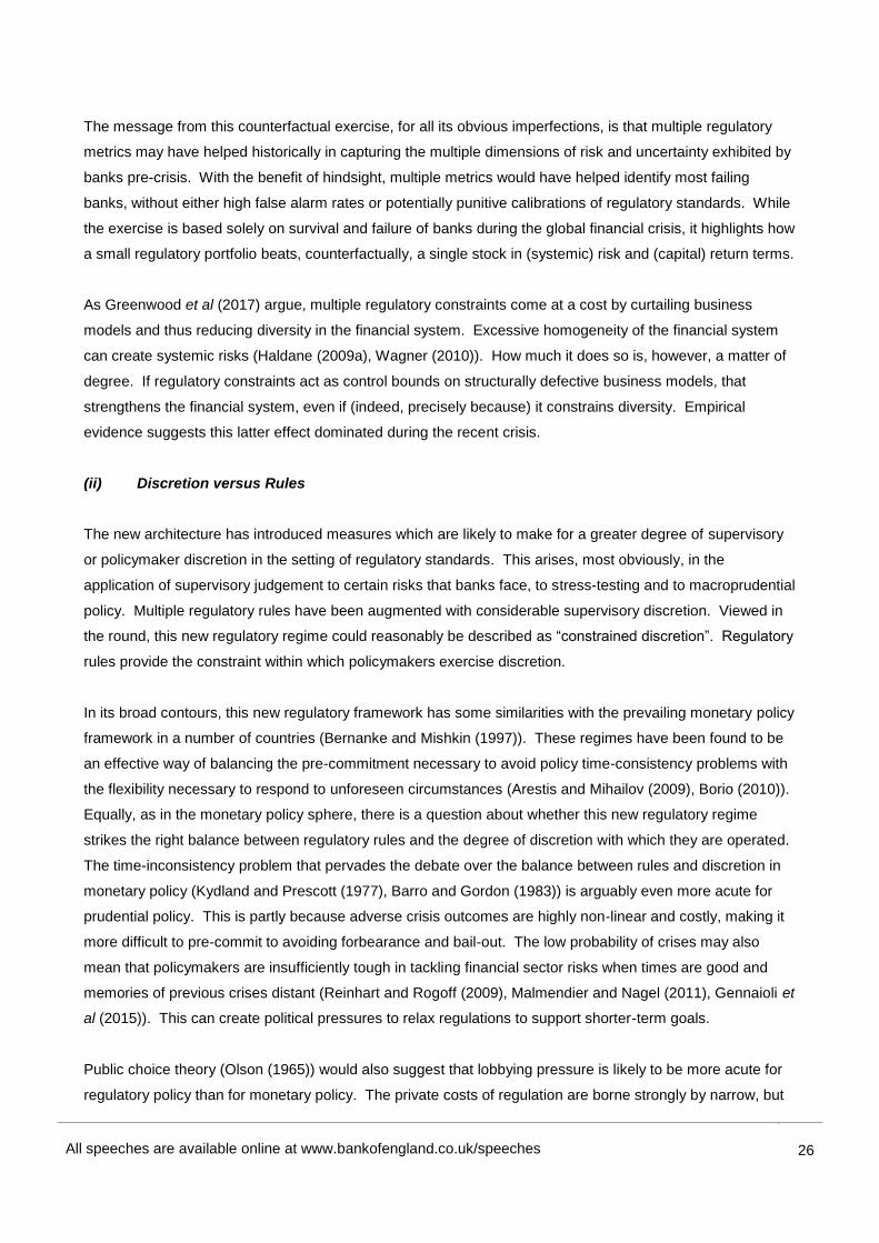
All speeches are available online at www.bankofengland.co.uk/speeches
26
26
The message from this counterfactual exercise, for all its obvious imperfections, is that multiple regulatory
metrics may have helped historically in capturing the multiple dimensions of risk and uncertainty exhibited by
banks pre-crisis. With the benefit of hindsight, multiple metrics would have helped identify most failing
banks, without either high false alarm rates or potentially punitive calibrations of regulatory standards. While
the exercise is based solely on survival and failure of banks during the global financial crisis, it highlights how
a small regulatory portfolio beats, counterfactually, a single stock in (systemic) risk and (capital) return terms.
As Greenwood et al (2017) argue, multiple regulatory constraints come at a cost by curtailing business
models and thus reducing diversity in the financial system. Excessive homogeneity of the financial system
can create systemic risks (Haldane (2009a), Wagner (2010)). How much it does so is, however, a matter of
degree. If regulatory constraints act as control bounds on structurally defective business models, that
strengthens the financial system, even if (indeed, precisely because) it constrains diversity. Empirical
evidence suggests this latter effect dominated during the recent crisis.
(ii) Discretion versus Rules
The new architecture has introduced measures which are likely to make for a greater degree of supervisory
or policymaker discretion in the setting of regulatory standards. This arises, most obviously, in the
application of supervisory judgement to certain risks that banks face, to stress-testing and to macroprudential
policy. Multiple regulatory rules have been augmented with considerable supervisory discretion. Viewed in
the round, this new regulatory regime could reasonably be described as “constrained discretion”. Regulatory
rules provide the constraint within which policymakers exercise discretion.
In its broad contours, this new regulatory framework has some similarities with the prevailing monetary policy
framework in a number of countries (Bernanke and Mishkin (1997)). These regimes have been found to be
an effective way of balancing the pre-commitment necessary to avoid policy time-consistency problems with
the flexibility necessary to respond to unforeseen circumstances (Arestis and Mihailov (2009), Borio (2010)).
Equally, as in the monetary policy sphere, there is a question about whether this new regulatory regime
strikes the right balance between regulatory rules and the degree of discretion with which they are operated.
The time-inconsistency problem that pervades the debate over the balance between rules and discretion in
monetary policy (Kydland and Prescott (1977), Barro and Gordon (1983)) is arguably even more acute for
prudential policy. This is partly because adverse crisis outcomes are highly non-linear and costly, making it
more difficult to pre-commit to avoiding forbearance and bail-out. The low probability of crises may also
mean that policymakers are insufficiently tough in tackling financial sector risks when times are good and
memories of previous crises distant (Reinhart and Rogoff (2009), Malmendier and Nagel (2011), Gennaioli et
al (2015)). This can create political pressures to relax regulations to support shorter-term goals.
Public choice theory (Olson (1965)) would also suggest that lobbying pressure is likely to be more acute for
regulatory policy than for monetary policy. The private costs of regulation are borne strongly by narrow, but

All speeches are available online at www.bankofengland.co.uk/speeches
27
27
powerful, interest groups in the financial industry. And while higher than target inflation is quickly observable,
it may be very difficult to judge in real time that regulation is insufficiently stringent given the difficulties of
quantifying the probability of future financial crises.
These arguments point to the need for strong institutional frameworks, supported by clear mandates,
objectives and instruments, to deliver financial stability policy. Indeed, on conceptual grounds, the need for
such a framework appears to be at least as strong, if not stronger, than for monetary policy. They also
support the case for clarity in the application of these regulatory policies.
Not least given its newness, there may be further to go clarifying the motivation behind macroprudential
interventions and the circumstances which might justify different macroprudential instruments - in short, in
defining and refining the macroprudential policy reaction function. The UK’s Financial Policy Committee has
made some progress in this area, most notably in setting out its strategy for using the countercyclical capital
buffer (Bank of England (2016a)). A discussion of the principles underlying the UK’s approach to
macroprudential policy can be found in Brazier (2017a).
The benefits of pursuing this path are clear from monetary policy experience (Brazier (2015)). Increasing the
predictability of policy can enhance the ex-ante signalling and expectations channels of regulatory policy, as
has been achieved in relation to monetary policy (Bernanke and Mishkin (1997)). It enhances ex-post
accountability to stakeholders, political and societal. And it reduces the potential behavioural biases
otherwise associated with discretionary decision-making and which have been found in the past to affect
discretionary regulatory policy, including regulatory capture (Dal Bó (2006)) and defensive decision-making
(Gigerenzer (2014)).
At the same time, there is clearly a balance to be struck. As Greenwood et al (2017) argue, strict
rules-based systems are likely to be arbitraged and exploited by banks. For example, recent theoretical work
and experimental evidence suggests remuneration contracts can be restructured to recreate the excessive
risk-taking incentives that new rules seek to reduce (Thanassoulis and Tanaka (2017), Harris et al
(forthcoming)).
These arguments make it difficult to specify strict regulatory rules for all seasons. They point to the need for
a forward-looking, horizon scanning approach with scope for supervisory judgement and macroprudential
discretion (BCBS (2017)). This does not, however, obviate the potential benefits from seeking, over time, to
specify clearer mandates and regulatory reaction functions, especially on the macroprudential front.
Incentives and Arbitrage
The empirical exercise in the previous section looked at how a set of regulatory standards, applied
counterfactually, might have done in spotting stress among a set of banks. Plainly, any such counterfactual

All speeches are available online at www.bankofengland.co.uk/speeches
28
28
exercise is subject to significant caveats. The most important of these is that it cannot take account of how
changes in the regulatory regime might themselves have reshaped risk-taking incentives at the time. This
Lucas Critique plainly looms large in the field of financial regulation.
Financial regulation, like any tax, is very likely to change the behaviour of the party subject to it. This is
neither surprising nor, necessarily, undesirable. Indeed, sometimes it is the precise purpose of the
regulation in the first place. For example, average risk weights on assets held in the trading book have
increased by 45% across a sample of major UK banks between 2006 and 2013. Partly in response, trading
books have shrunk by, on average, 24% across these banks and by 45% across the world’s G-SIBs. This
was an intended, and probably desirable, behavioural response to a necessary recalibration of regulatory
standards.
That is not to say, however, that all behavioural adjustments are either exactly as intended or desirable.
This is particularly the case when these responses seek to avoid regulation entirely – so-called regulatory
arbitrage. Risk, like energy, does not disappear into the ether. It is typically conserved, at least to some
degree. In response to tighter financial regulation, risk is likely to change shape or location, often both.
This is not just a conceptual point. The history of financial regulation can be seen as an on-going,
evolutionary race to adjust regulatory rules to limit avoidance incentives (Haldane (2013)). The first Basel
Accord (“Basel I”) was a direct response to cross-border regulatory arbitrage. Basel II came largely as the
result of standardised approaches to risk measurement being arbitraged. And Basel III came in part as a
response to both risk models, and the Basel framework itself, being arbitraged. This race has been
characterised as “bloodhounds in pursuit of greyhounds” (Eichengreen (2009)). Regulators need both to
learn from past experience and to anticipate future opportunities for avoidance (Woods (2017)).
The arbitrage problems faced by the bloodhounds were well-exemplified in the run-up to the global financial
crisis. These included the migration of activity and risk to unregulated “shadow banks” (Adrian and Ashcraft
(2012)); the hard-wiring of rating agency risk assessments into the regulatory engine (Edmonds (2016)); the
payment of bank CEOs in common equity encouraging “gambling for resurrection” (IMF (2014)); and the
implicit subsidies conferred on “too-big-to-fail” institutions, encouraging them to become larger and more
complex and connected still (FSB (2013b)).
Another example of these incentive effects came in the area of capital regulation. Whichever risk-weighting
scheme is in place, it is likely to give rise to incentives to adjust asset positions to maximise profits. For
example, if the regulatory constraint takes the form of a leverage ratio there are incentives to alter the
composition of assets towards those with higher risk weights – though the evidence on such “risk-shifting” is
mixed (Sheldon (1996), Furlong (1988)). Contrarily, if assets are risk-weighted and determined by banks’
internal models, there are incentives to lower modelled risk weights over time (Mariathasan and Merrouche
(2014)). In short, when setting capital standards for banks, there is a two-sided incentive problem.

All speeches are available online at www.bankofengland.co.uk/speeches
29
29
Pre-crisis, both incentives were at play, albeit to differing degrees in different parts of the global financial
system. In the US, where a leverage ratio was in operation and often the binding constraint, there were
incentives for banks to seek higher-risk assets rather than expand balance sheets (Chart 20). In Europe,
without a leverage ratio but with risk-based capital standards, there were incentives for banks to expand
balance sheets and shade downwards risk weights. Canadian banks’ incentives sat somewhere in between.
Some recent studies have looked at these behavioural shifts in greater detail. During the euro-area crisis,
banks increased their exposure toward higher risk government bonds, which carried no capital requirement
(Acharya and Steffen (2015)). And following the Lehman crisis, German banks reduced their corporate
lending less when the capital requirement was set under the standardised approach (Behn, Haselmann,
Wachtel (2016)). In the UK, higher risk mortgages shifted towards lenders whose capital requirements were
less risk-sensitive after the introduction of Basel II (Benetton et al (2017)).
Recent research has considered how the leverage ratio announcement affected behaviour among a panel of
over 650 European banks (Acosta-Smith et al (2017)). It finds a significant increase in risk-taking among
those banks for whom the new regime was a binding constraint. This risk-taking was greater, the further
these banks were from meeting the new 3% threshold: banks with leverage ratios of 1.5%, 2% and 2.5%
were found to increase their risk-taking by 3.4, 2.3 and 1.1 percentage points of risk-weighted assets
respectively. This is clear empirical evidence of the risk-shifting channel at work.
This is only, however, one side of the risk equation. There were two mitigating factors on the other side.
First, a rise in the leverage ratio also boosts these banks’ capital. Once translated into default probabilities,
Acosta-Smith et al (2017) find that the second effect swamps the first: a one percentage point rise in the
leverage ratio raises the odds ratio (on banks being in distress versus safe) through risk-shifting by 1-3.5%.
But the reduction in the odds ratio from lower leverage is close to 40-50%.
Second, the leverage regime is not a replacement for the risk-weighted capital regime but an addition to it.
The capital regime places an automatic upper-bound on the extent to which banks can increase their
risk-weighted assets. In other words, the capital ratio regime places constraints on incentives to risk-shift.
Conversely, the leverage ratio can serve as an effective constraint on incentives to game or shade risk
weights. Risk-taking incentives are, in effect, book-ended by the leverage and capital constraints.
From an incentives perspective, if regulatory arbitrage incentives are two-sided, so too should be the
constraints needed to straightjacket that behaviour. That is another way of rationalising the “multi-polar”
regulatory regime operating internationally. When it comes to calibration, this means leverage and capital
ratios need to be jointly determined to prevent incentives skewing in one or other direction. This is the
approach in the UK when setting capital and leverage constraints (Bank of England (2015a)).

All speeches are available online at www.bankofengland.co.uk/speeches
30
30
There are other means of constraining adverse incentives. Incentives to game risk weights can be
constrained by imposing floors and/or by using standardised approaches for certain categories of assets.22
Some countries already make use of such approaches, including the US, the UK, Germany, France and
Spain. The stress-testing regimes operating in a number of countries are also a way of cross-checking, and
backstopping, the models used by banks. In a world of uncertainty as well as risk, having this portfolio of
approaches for dealing with avoidance incentives - some discretionary, others rule-like - makes sense.
Evidence on the incentive effects of financial regulation is almost always drawn from looking at banks’
experience either side of a change in policy. By then, however, any unintended or undesirable
consequences of this change will already have been felt. Regulatory policy is in a perpetual catch-up loop,
the bloodhounds in pursuit of the greyhounds.
In an ideal world, it would be possible to gauge in advance how a regulatory change may reshape incentives,
in particular risk-taking or regulatory-avoiding incentives. One approach to doing so is to use experimental
methods. Experiments have previously been used to examine how different pay structures affect loan
officers’ risk assessment and lending decisions (Cole, Kanz and Klapper (2015)). They have also been used
to examine the effect of specific interventions on behaviour in other areas of public policy (Halpern (2015)).
Recently, the Bank of England has conducted a lab experiment to assess how the design of pay regulation
may affect risk-taking behaviour and project search effort (Harris et al (forthcoming)). Specifically, the
experiment was designed to examine how caps on bonuses and “malus” (bonuses that are not paid out if, for
example, performance falters in subsequent years) might affect individuals’ risk choices and efforts to seek
out the best projects. The experiment showed evidence that, while both schemes tend to reduce risk-taking,
they could be arbitraged relatively easily by introducing absolute or relative performance targets. There was
also some evidence that a bonus cap might reduce incentives to search for good projects.
The Bank of England is considering extending this experimental approach to a wider range of policy design
questions and a wider range of financial market participants - risk-takers and risk-managers. In principle, this
approach might provide some early indications of how new regulation might reshape risk incentives,
including arbitrage incentives, which could help in recrafting regulation before it is introduced.
Macroprudential Policy
One of the greatest intellectual errors made in the run-up to the crisis was a classic “fallacy of composition”:
it was assumed that the resilience of individual financial institutions was both a necessary and sufficient
condition to ensure the resilience of the financial system as a whole. Events during the crisis, and
22
See BCBS (2016): http://www.bis.org/bcbs/publ/d362.pdf and BCBS (2013b): http://www.bis.org/publ/bcbs258.pdf

All speeches are available online at www.bankofengland.co.uk/speeches
31
31
subsequent theoretical and empirical work, has shown that the resilience of individual firms is neither
necessary nor sufficient for the mitigation of systemic risk (Masera (2014), Crockett (1996)).
Out of this intellectual vacuum, a new framework for regulation has been born – macroprudential regulation.
This explicitly recognises the links that might tie together individual nodes in the financial system. These
might arise from correlated asset exposures, the type of which has historically emerged during the upswings
and downswings of the credit cycle (Aikman et al (2015)). Or they might emerge from financial exposures,
on- or off-balance sheet, between intermediaries operating in the global financial web (Haldane and May
(2011), Arinaminpathy, Kapadia and May (2012)).
Over the past decade, a lot has been written in the area of macroprudential policy (Galati and Moessner
(2013), Aikman et al (2013), Freixas et al (2015)). A sizeable number of countries are now undertaking
macroprudential policy in some shape or form. Table 5 in the Annex provides a rough summary of current
international macroprudential practices (for a more comprehensive overview, see Cerutti et al (2017)). By
any historical metric, however, macroprudential policy remains a fledgling framework. Understandably, many
of its key facets remain contentious. And the macroprudential policies put in place internationally so far are
more notable for their differences than their similarities. This is providing a diverse body of case law.
We discuss two key aspects of this framework: its appropriate objectives; and the choice of instruments.
Objectives of Macroprudential Policy
The Bank of England entered the debate on the potential role of macroprudential policy in a discussion paper
published in 2009 (Bank of England (2009)). That paper cast the debate on the potential objectives of such
a regime as a choice between ‘protecting banks from the cycle’ and ‘protecting the economy from the banks’.
Macroprudential policy could focus narrowly on building resilience in the financial system in a dynamic way,
so that it was better able to absorb large adverse shocks. Or it could pursue the broader and bolder
objective of smoothing the swings in debt and asset prices associated with the financial cycle.
The subsequent academic literature has usefully refined how we think about these goals of a
macroprudential regime. One fruitful strand has focused on the pecuniary externalities generated by
fire-sales in asset markets (Lorenzoni (2008), Jeanne and Korinek (2010), Bianchi and Mendoza (2010),
Benigno et al (2013)). Collateralised borrowing leads to externalities because individual borrowers do not
internalise the fact that increasing debt in good times raises the likelihood they will be forced to sell assets
following adverse shocks, pushing prices lower, tightening collateral constraints and exacerbating downturns.
These feedback and amplification loops can mean that private borrowing in good times is greater than a
social planner would choose, facing the same constraints. That is the theory. Experience during the crisis
tends to support the importance of these transmission channels. When highly-levered banks were forced to

All speeches are available online at www.bankofengland.co.uk/speeches
32
32
sell illiquid assets at highly discounted prices, this lowered valuations further and tightened constraints for
other banks (Brunnermeier (2009)). This contributed to the depth and duration of the economic downturn.
Another strand of the literature has examined whether unlevered investors may also be prone to this fire-sale
mechanism. This is a question of rising importance given the rapid growth in open-ended investment funds
since the crisis. In Feroli et al (2014), asset managers are motivated by their relative ranking. This
generates a feedback loop in which falling asset prices incentivise further selling for fear of diverging from
the pack (Morris and Shin (2016), Vayanos and Woolley (2013)). This channel is amplified if investors
perceive there to be a first-mover advantage in withdrawing funds, generating ‘run-like’ behaviour (Goldstein,
Jiang and Ng (2017), Chen, Goldstein and Jiang (2010), Morris, Shim and Shin (2017)).
A recent paper by Bank of England colleagues (Baranova et al (2017)) provides a framework for quantifying
the risks posed by investment funds in corporate bond markets (see also Ceterolli et al (2016)). In their
model, investors act pro-cyclically, withdrawing funds when corporate bond prices fall and causing
investment funds to make a first-round of asset sales. Dealers provide liquidity, but require a further fall in
price as compensation. This leads to further redemptions and further asset sales, amplifying the fall in price.
Chart 21 shows that this amplification effect can be quantitatively significant: weekly redemptions from bond
funds of 1% of total net assets, similar to the level observed at the peak of the crisis, increase the liquidity
premium in bond spreads by 40 basis points. Moreover, redemptions of as little as 1.3% of total assets
exhaust the dealer’s capacity to intermediate trades, leading to a market ‘freeze’.
In a similar spirit, Braun-Munzinger et al (2016) develop an agent-based model of the corporate bond market
comprising a market maker, fund traders and fund investors. They find that funds pursuing similar trading
strategies can exacerbate price movements and contribute to the pro-cyclicality of financial markets.
Additionally, the growth of passive investments may have both positive and negative effects on volatility:
they decrease yield volatility on average, but can increase the likelihood of large dislocations after shocks.
While this fire-sale mechanism applies most directly to financial intermediaries with marked-to-market
balance sheets, and funds that can be redeemed at short notice, a similar dynamic can operate if there are
forced sales by owners of, or investors in, real estate who are credit-constrained borrowers.
This, too, can drive prices lower in a feedback loop. Some of these mechanisms were in play recently
among UK real estate investment vehicles following the EU referendum result (Bank of England (2016b)).
A related, but distinct, mechanism through which financial frictions can affect the wider economy is through
aggregate demand externalities. In Korinek and Simsek (2016), credit-constrained households de-lever
sharply when an adverse shock hits. If the shock is large enough, the resulting fall in aggregate demand can
push the economy into a liquidity trap with interest rates constrained at the effective lower bound. In this
environment, macroprudential policies that slow the build-up of household leverage ex-ante can be

All speeches are available online at www.bankofengland.co.uk/speeches
33
33
welfare-improving in avoiding this outcome. Farhi and Werning (2016) also offer a model of macroprudential
policy in the face of aggregate demand externalities.
Another strand of the literature emphasises behavioural sources of pro-cyclicality. For example, powerful
narratives, such as a collective belief in a ‘new paradigm’, might manifest themselves in over-exuberance in
the financial system (Tuckett (2011), Shiller (2017)). Myopia about risk might also drive excessive
risk-taking, especially as memories of past financial crises fade (Guttentag and Herring (1986), Herring
(1998), Haldane (2009b), Gennaioli, Schleifer and Vishny (2012)). And such behaviour might be amplified
by contracts that reward short-term performance excessively and by herding in financial markets (Avery and
Zemsky (1998), Lakonishok et al (1992), Bikhchandani and Sharma (2001)). Aikman, Nelson and Tanaka
(2015) show how reputational concerns and peer benchmarking can drive credit cycles.
The case for macroprudential interventions to address build-ups in leverage also has empirical support.
Mian and Sufi (2010) argue that the persistence of the decline in US GDP after the crisis was caused by
excessive household leverage. Jordà et al (2013) report that credit booms not only increase the likelihood
and severity of financial crises, but also make normal recessions more painful. A one standard deviation
increase in ‘excess credit’ results in real GDP per capita being 1.5% lower five years after a normal
recession.23
Bunn and Rostom (2015) find that more highly indebted groups of households made larger cuts
in spending following the financial crisis. And Bailey et al (forthcoming) exploit Facebook data to identify how
social interactions can drive contagious risk-taking in the US housing market.
In summary, the market failures associated with fire-sale externalities and behavioural tendencies which can
drive short-termism provide a strong case for a macroprudential regulator with an objective of preserving the
dynamic resilience of the financial system, both among banks and, prospectively, among non-banks. No
less compelling, however, is the evidence, both micro and macro, linking credit booms to aggregate demand
externalities. That, in turn, provides a rationale for pre-emptive macroprudential interventions to avoid
excessive inflation of credit and asset prices in the first place.
Instruments of Macroprudential Policy
The Bank of England’s second public foray into the macroprudential policy debate was a 2011 discussion
paper on elements of the macroprudential toolkit (Bank of England (2011)). That paper described 12 distinct
macroprudential tools (see also CGFS (2010, 2012), Hanson et al (2011) and ESRB (2015) for discussions
of macroprudential instruments). The majority of these targeted different aspects of banks’ balance sheets
including: the countercyclical capital buffer (CCyB); sectoral capital requirements (SCRs); leverage ratio
buffers; dynamic provisions; and liquidity buffers.
23
Defined as the rate of change of aggregate bank credit (domestic bank loans to the nonfinancial sector) relative to GDP, relative to its mean, from previous trough to peak.

All speeches are available online at www.bankofengland.co.uk/speeches
34
34
Other potential macroprudential instruments included those aimed at influencing lending standards - for
example, through setting loan to value limits (LTV), loan to income limits (LTI) or margining requirements on
collateralised borrowing in financial markets. A third set of potential instruments focused on making market
infrastructures more resilient and improving financial market practices – for example, by mandating central
clearing, through trading venue design and through enhanced disclosure requirements.
So how has thinking on macroprudential instruments moved forward in the period since? Chart 22
documents the use of different types of macroprudential tool over the past decade in a panel of advanced
economies.24
Perhaps contrary to expectations, the majority of interventions have fallen into the “lending
standards” category, a group that includes LTI and LTV requirements. By numbers, such actions account for
around two-thirds of overall macroprudential actions over the period since 2010.
At the other end of the spectrum is the CCyB. That has only been used by 6 countries to date. This is
surprising given that it is the only tool that has a well-defined operating framework internationally and which
includes jurisdictional reciprocity. A potential explanation is that the Basel guidelines suggest the buffer
should be activated when excess credit growth threatens an increase in system-wide risk. The majority of
advanced countries have not come close to experiencing aggregate credit booms in the post-crisis period.
When it comes to assessing the efficacy of these tools, it has largely been a case of ‘learning by doing’.
Cerutti et al (2017), Kuttner and Shim (2013), Crowe et al (2013) and Boar et al (2017) provide evidence on
the impact of tools using cross-country panel studies. Aikman et al (forthcoming) and Banerjee and Mio
(2017) study the UK’s experience with the CCyB and with macroprudential liquidity actions respectively. And
He (2013) considers the impact of the HKMA’s use of LTV limits. Overall, however, the evidence base on
the transmission of macroprudential tools remains fairly slim.
There is also relatively little guidance from the literature on tool strategy, selection and interaction. One
exception is work assessing the role of monetary policy in leaning against financial cycles. A paper by the
Federal Reserve Board (Ajello et al (2016)) analyses the costs and benefits of using interest rates to lean
against vulnerabilities in the financial system. In the baseline calibration of their model, the costs of using
monetary policy in this way are large relative to the benefits: the optimal adjustment in interest rates in the
face of financial stability risks is in the order of 3 basis points.
While the adjustment to interest rates can be larger – up to 75 basis points - if alternative assumptions are
made about cost of crises and the sensitivity of crisis risk to monetary policy, the calibrations required to
deliver these outcomes are extreme. Svensson (2017) argues that the costs of using interest rates to lean
against financial crisis risk are likely to be greater still if one takes into account that doing so will make the
economy weaker at the point a crisis strikes and hence might actually worsen its severity.
24
We would like to thank Karam Shergill and Rhiannon Sowerbutts for collecting these data.

All speeches are available online at www.bankofengland.co.uk/speeches
35
35
Aikman et al (2016) analyse empirically the joint non-linear dynamics of credit, financial conditions and
monetary policy in the United States. They find that the transmission mechanism of monetary policy to
long-term yields is blunted in high credit states. This suggests that attempts to lean against the wind with
monetary policy when credit is already elevated may be futile. Filardo and Rungcharoenkitkul (2016), by
contrast, find benefits from using monetary policy to ‘lean’ when the evolution of financial imbalances is
extremely persistent. But the general consensus is against deploying monetary policy, at least in an activist
way, for financial stability purposes given its limited efficacy and potential real-economy costs.
One recent paper that addresses issues of CCyB strategy is Aikman, Giese, Kapadia and McLeay
(forthcoming). Developing Ajello et al’s (2016) approach, the authors study an economy in which
policymakers face a trade-off between stabilising inflation and output today versus keeping a lid on financial
stability risks which threaten a crisis tomorrow. The optimal strategy is to adjust the CCyB in line with
forward-looking indicators of crisis risk – credit growth in their model – but to relax (tighten) the CCyB relative
to this plan if output is below (above) its target level. This strategy dramatically improves the inter-temporal
trade-off facing a policymaker relative to the case where monetary policy is the only tool (Chart 23). Indeed,
this is consistent with the Bank of England MPC’s guidance that monetary policy should be the ‘last line of
defence’ in the presence of financial stability risks (Bank of England (2013)).
The dashed lines show the steep trade-off facing a policymaker with a monetary policy tool only. Attempts to
reduce the crisis probability with higher interest rates entail significant costs for current output and inflation.
The solid lines show how this trade-off improves when the CCyB is added to the instrument set, even under
conservative assumptions about the impact of the CCyB on the economy’s productive capacity. The
variation in the CCyB required to deliver these benefits can be large. Given the historical distribution of
shocks, the standard deviation of the CCyB is around 2 percentage points.
A final strand of the literature has analysed whether the presence of macroprudential policy gives rise to
coordination problems with monetary policy. For example, De Paoli and Paustian (2017) study a
non-cooperative game between monetary and macroprudential authorities and find coordination problems to
be significant following cost-push shocks in cases where objectives do not overlap. But they also find that a
leadership structure in which macroprudential policy moves first – or is varied at a lower frequency than
monetary policy given that financial vulnerabilities build slowly – mitigates these coordination problems.
Future Research and Policy
Financial regulation has undergone a fundamental rethink and reform since the global financial crisis. By
most accounts and on most evidence, that has resulted in a financial system which is more resilient than in
the past, better equipped to head-off market frictions and failures of various kinds, better attuned to various
adverse incentive effects, and better able to safeguard risks which imperil the financial system as a whole. It

All speeches are available online at www.bankofengland.co.uk/speeches
36
36
is a regime of “constrained discretion”, comprising a portfolio of regulatory measures calibrated, albeit
roughly, to equate societal costs and benefits. That’s the easy bit.
The hard bit is what happens next. Not least given the scale of regulatory change over the past decade, this
new regulatory framework will plainly need to adapt in the period ahead in the light of the new evidence,
experience and incentives associated with operating it. This paper has discussed some of those issues.
From a potentially very long list, we conclude by highlighting some of the areas where we think further
research and practical exploration might be useful in the future debate on regulatory reform.25
(a) Optimal Levels of Capital: One of the most animated, on-going areas of regulatory debate is whether
capital standards have been appropriately calibrated. Relative to the pre-crisis LEI study, current levels of
capital requirements in most countries are below that calibration. The single most important reason for that
is because the LEI study did not take into account the potential impact of non-equity sources of capital,
specifically TLAC, in reducing the impact and probability of crisis. The key question, then, is whether these
instruments prove to be as loss-absorbing in future situations of stress where bail-in becomes necessary.
This issue is particularly relevant when it involves systemically-important institutions or sets of institution,
when the costs of bailing-in (and bailing-out) are large and lumpy. At this early stage, the jury must still be
out. On the one hand, historical evidence on bailing-in different types of notionally loss-absorbing bank
liabilities in situations of systemic stress has not been encouraging, reflecting the acuteness of the
time-consistency problem facing the authorities in these cases. On the other, new statutory resolution
arrangements are much stronger than ever previously, and statutory TLAC requirements are now prescribed
in advance. This means next time could plausibly be different. Given its importance to the overall capital
calibration, this issue deserves further empirical and theoretical consideration.
(b) Multi-Polar Regulation: The new regulatory framework is a different beast than its predecessors in terms
of the number, complexity and discretionary nature of the constraints it imposes. There are good conceptual
and empirical grounds for such a portfolio approach in insuring against future risks and, in particular,
uncertainties. And from a risk- and uncertainty-averse social welfare perspective, even a marginally
over-identified system might, in general, be preferable to a marginally under-identified one, if recent crisis
experience is any guide. Indeed, that is the essence of robust control. Ultimately, however, the past is
another country. There are legitimate questions to answer about whether multiple regulatory constraints
could lead to excessive homogeneity and inefficiency in the financial system. And arbitrage is an
ever-present threat, even with multiple regulatory metrics. This is an area where further research and
practical experience with operating the new regime will be essential in gauging whether there is scope for
streamlining, provided the resulting regulatory regime remains robust to the radical uncertainty that
necessarily affects any complex, adaptive system such as finance.26
25
See also, Calomiris (2017), Duffie (2017), Greenwood et al (2017). 26
FSB (2017e), for example, describes a Policy Evaluation Framework to achieve efficient resilience.

All speeches are available online at www.bankofengland.co.uk/speeches
37
37
(c) Models of Financial Stability: In a world of monetary, macroprudential and microprudential policy, all
having an impact on the economy and on the financial system, there is an increased onus on developing
quantitative frameworks which enable us to understand their impact, individually and collectively, and their
interaction (Bank of England (2015b)). That calls for models able to capture quantitatively monetary,
financial and regulatory channels of transmission and the feedback mechanisms between them. Progress
has been made, in particular since the crisis, in developing macro-models with an explicit financial sector
which can capture rich, two-way feedbacks between the economy and financial system (for example,
Brunnermeier et al (2012), Brunnermeier and Sannikov (2014)). There has been progress, too, in
developing models of systemic risk which assign macroeconomic factors, and within-system feedbacks, a
prominent role (Greenwood et al (2014), Cont and Schaanning (2017)). Yet we are still probably in the
foothills when developing a unified framework for bringing these factors together in one place, a framework
that could capture the rich feedback and amplification mechanisms that operate in practice and a model
which could then serve as a test-bed for each of the three arms of policy. Indeed, it could be that a single,
Holy Grail, framework is infeasible or indeed undesirable.
(d) Future of Stress-Testing: Bank stress testing has evolved considerably since the financial crisis and is
now a cornerstone of the regulatory regime in many jurisdictions. The direction of travel necessary to enrich
these tests, and to make them truly macroprudential, is to incorporate feedback effects that can amplify the
actions of individual institutions at the system-wide level (Demekas (2015), Brazier (2015), Tarullo (2016)) –
feedbacks, for instance, that result from fire-selling assets, hoarding liquidity and counterparty risk.27
A
natural consequence is that we might need to extend the field of vision for such simulations to include non-
bank parts of the financial system. Non-bank sources of systemic risk proved to be potent during the crisis,
in particular among shadow banks. As regulation has squeezed the banking system, there has been further
migration of financial activity into the shadows, particularly within Europe. What was once credit and funding
risk on the balance sheets of banking firms is metamorphosing into market and liquidity risk on the balance
sheets of funds and investment vehicles of various types (Stein (2013)). Understanding these risks calls for
new and enhanced surveillance tools. Systematic, market-wide stress simulations might be needed to
capture new market and liquidity risks and their propagation across different financial institutions and
markets (Brazier (2017b)). The same considerations apply to key pieces of the financial infrastructure, in
particular central counterparties (Cœuré (2017), Duffie (2017)). As a potentially new “too big to fail” entity,
they too need to be stress-tested and their resolution plans agreed and implemented. This is a whole new
risk-management agenda, where work has only just begun in earnest.
(e) Market-Based Finance: The emergence of a large and diverse shadow banking system, both prior to the
crisis in the US and subsequent to it elsewhere around the world, plainly poses both considerable
opportunities and potential threats to financial stability. So-called market-based finance provides the
financial system with a second, non-bank, engine on which to fly which could be beneficial in a diversity
27
For example, the results of the Bank of England’s 2014 stress test found that risk-weight procyclicality was a significant contributor to
the change in capital ratios in the stress test scenario (Bank of England (2014)).

All speeches are available online at www.bankofengland.co.uk/speeches
38
38
sense. Nonetheless, it also gives rise to potentially new sources of systemic risk and contagion, as risks
change shape and location. The FSB has made significant progress in progressing the regulatory debate on
such matters (FSB (2017e)). Certainly, these trends carry implications for both the conduct of regulation and
for central bank procedures. A world of greater market and liquidity risk may call for different sets of
regulatory instrument than the bank-based solvency and liquidity metrics of Basel III. Market-based
instruments, such as margin requirements, may have a greater role to play (see, for example, ESRB (2017)).
It may also call for different types of market intervention by central banks – different markets, different
instruments, different counterparties. The crisis has already seen a mini-revolution in the design of liquidity
facilities by central banks. As the financial system changes shape, it seems plausible to think that further
change could be necessary. If so, that change would benefit from further research on the costs and benefits
of the extended regulatory and central bank safety net.
(f) The Macroprudential Policy Framework: As a still-fledgling framework, there are a wide range of
questions still surrounding the macroprudential framework. There is no settled, practical approach to defining
the breadth of objectives of a macroprudential regime. Should the potential for aggregate demand
externalities associated with a debt overhang in the household sector, for instance, fall under the purview of
a macroprudential authority? Nor, in the main, is there any settled approach to defining the appropriate set
of macroprudential instruments, whether for banks or especially for non-banks, or the optimal strategy for
their use to address emerging vulnerabilities. If household debt externalities are within scope, is it better to
deal with this risk by restricting mortgage lending directly via loan to income or loan to value limits, or by
adding a macroprudential overlay to risk weights on mortgages (Turner (2017))? This lack of a settled
approach has some benefits, in making for a diverse range of cross-country experiences. This is giving rise
to a period of “learning by doing” among regulators. It does, however, come at some cost. A regime without
especially well-defined objectives is likely to suffer greater problems of time-inconsistency. It may also
increase uncertainty among outside participants about the likely regulatory policy reaction function.
The direction of travel, over time, probably needs to be towards somewhat clearer constraints, and
somewhat more circumscribed discretion, if macroprudential regimes are to be effective, robust and
transparent.
(g) Political Economy of Financial Regulation: The scope and range of regulatory responsibilities assigned to
central banks and regulators have expanded materially during the course of the crisis. Accompanying that,
some of the new regulatory requirements and practices put in place are quite discretionary in nature,
including stress-testing and some other macroprudential measures. A number involve regulators making
overtly distributional choices, for example around access to credit. This takes central banks and reguIators
more explicitly into the political-economy realm than at any time in their recent (and perhaps distant) history.
It has probably also contributed to some people questioning the appropriate scope of central banking, its
degree of independence from the political process and from wider society and appropriate accountability
mechanisms. There is a debate to be had, an analytical debate, about the appropriate degree of discretion
to confer on regulators, to ensure they retain the flexibility they need to respond to events while ensuring

All speeches are available online at www.bankofengland.co.uk/speeches
39
39
their decisions are clear, transparent and unpolluted by behavioural biases and time-inconsistency problems.
There are also interesting issues to explore about how regulators explain and account for their decisions to
wider society, particularly when they have strongly distributional consequences. This is clearly unfinished
business.
(h) The Contribution of the Financial System to the Economy and to Society: One of the striking features of
the past several decades has been the rising share of financial services in measures of economy-wide
value-added and, in tandem, rising financial sector balance sheets as a fraction of GDP in a number of
economies. Sometimes this goes by the name “financialisation”. There are good reasons to think increasing
financial depth is a natural feature of economies as they grow and develop. Indeed, there is a fairly
well-established literature quantifying the boost to growth and productivity which arises from financial depth,
especially for developing countries (Levine et al (2000)). Latterly, however, the question has been asked
whether it is possible to have too much of a good thing. Some have asked why the cost of financial
intermediation continues to rise and what this might signal about the efficiency of financial services as an
industry (Friedman (2009), Philippon (2015)). Others have pointed to a possible U-shaped relationship
between measures of financial depth and productivity and growth (Cecchetti and Kharroubi (2012), Heil
(2017)). These questions have an important bearing on the contribution the financial system makes to the
economy and to society. They are also meta-questions for regulatory policy. They warrant further research.
(i) Financial Stability Implications of FinTech: Technologically-enabled innovation in financial services, or
FinTech, has grown rapidly in recent years. The FSB’s recent report contains a useful taxonomy of such
innovations (FSB (2017f)). With this development comes the promise of greater consumer choice, improved
access to credit for some borrowers, and greater efficiency and productivity in the traditional intermediary
sector. There are also potential resilience benefits from increasing diversity in the provision of financial
services (Carney (2017a)). While the sector is probably too small at present to pose a threat to financial
stability, there is ample historical experience of risks emerging rapidly in fast-growing sectors if left
unchecked. Such future risks might include: conventional vulnerabilities associated with excessive use of
leverage and maturity, liquidity and credit transformation; the emergence of new highly-interconnected
entities; and cyber and other operational risks. There is also the potential for these developments to make
traditional universal banks less resilient, if they are forced to rely on less stable funding sources, for example.
A challenge for policymakers is to ensure that the regulatory regime, and the wider policy framework –
including the scope of central banks’ liquidity facilities – adapts to keep pace with these developments
(Lagarde (2017)).

All speeches are available online at www.bankofengland.co.uk/speeches
40
40
Annex
Chart 1: Level of real GDP in the Great Recession and Great Depression
US
UK
Germany
France
Sources: ONS, Bank of England ‘Millennium of Data’ (2017), IMF WEO, Maddison Historical GDP Data and Bank calculations.
Notes: ‘Continuation of pre-crisis’ trend is a simple extrapolation of GDP beyond 2007 using the average GDP growth from 1998 to 2007
for each country.
The strong rebound in GDP growth for Germany following the Great Depression will partly reflect the armament period in the run-up to
World War II.
60
70
80
90
100
110
120
130
140
0 1 2 3 4 5 6 7 8 9 10
Great Depression (Year 0 = 1929)
Great Recession (Year 0 = 2007)
Continuation of pre-crisis trend (1998-07)
Years from start of crisis
Index, Year 0 = 100
90
100
110
120
130
140
0 1 2 3 4 5 6 7 8 9 10
Great Depression (Year 0 = 1929)
Great Recession (Year 0 = 2007)
Continuation of pre-crisis trend (1998-07)
Years from start of crisis
Index, Year 0 = 100
60
70
80
90
100
110
120
130
140
150
0 1 2 3 4 5 6 7 8 9 10
Great Depression (Year 0 = 1929)
Great Recession (Year 0 = 2007)
Continuation of pre-crisis trend (1998-07)
Years from start of crisis
Index, Year 0 = 100
60
70
80
90
100
110
120
130
140
0 1 2 3 4 5 6 7 8 9 10
Great Depression (Year 0 = 1929)
Great Recession (Year 0 = 2007)
Continuation of pre-crisis trend (1998-07)
Years from start of crisis
Index, Year 0 = 100

All speeches are available online at www.bankofengland.co.uk/speeches
41
41
Chart 2: Government debt to GDP ratio in the Great Recession and Great Depression
US
UK
Germany
France
Sources: Bank of England ‘Millennium of Data’ (2017), IMF Historical Public Debt Database and Bank calculations.
Notes: Data for French government debt between 1934 and 1948 is not available in the IMF dataset.
0
5
10
15
20
25
30
35
40
0 1 2 3 4 5 6 7 8 9 10
Great Depression (Year 0 = 1929)
Great Recession (Year 0 = 2007)
Change in government debt to GDP ratio from start of crisis (percentage points)
-20
-10
0
10
20
30
40
50
60
0 1 2 3 4 5 6 7 8 9 10
Great Depression (Year 0 = 1929)
Great Recession (Year 0 = 2007)
Change in government debt to GDP ratio from start of crisis (percentage points)
Years from start of crisis
-4
-2
0
2
4
6
8
10
12
14
0 1 2 3 4 5 6 7 8 9 10
Great Depression (Year 0 = 1929)
Great Recession (Year 0 = 2007)
Change in government debt to GDP ratio from start of crisis (percentage points)
Years from start of crisis
0
5
10
15
20
25
30
35
40
0 1 2 3 4 5 6 7 8 9 10
Great Depression (Year 0 = 1929)
Great Recession (Year 0 = 2007)
Change in government debt to GDP ratio from start of crisis (percentage points)
Years from start of crisis
Years from start of crisis

All speeches are available online at www.bankofengland.co.uk/speeches
42
42
Chart 3: Compliance with EDTF disclosure
Sources: Progress reports of the Enhanced Disclosure Task Force from 2013, 2014, and 2015; Bank calculations
Chart 4: G-SIB and D-SIB Tier 1 capital ratios
Sources: S&P Capital IQ and Bank calculations
Notes: Weighted average based on a sample of 189 banks which are systematically important as of 2016. Yearly is defined as the
fiscal year of reporting of the individual banks. Tier 1 Capital Ratio = Tier 1 Capital/Risk Weighted Assets
0%
10%
20%
30%
40%
50%
60%
70%
80%
90%
100%
201420132012Pre-EDTFReport
Aggregate implementation UK implementation
0
2
4
6
8
10
12
14
16
2006 2007 2008 2009 2010 2011 2012 2013 2014 2015 2016
Per cent
Total GSIBs DSIBs

All speeches are available online at www.bankofengland.co.uk/speeches
43
43
Chart 5: G-SIB and D-SIB leverage ratios
Notes: Weighted average based on a sample of 189 banks which are systematically important as of 2016. Yearly is defined as the
fiscal year of reporting of the individual banks.
Chart 6: Major UK banks’ regulatory capital, MREL resources and requirements, % RWA (2011-2022)
Sources: FSA regulatory returns, MREL+ returns, Bank calculations
0
1
2
3
4
5
6
7
8
2006 2007 2008 2009 2010 2011 2012 2013 2014 2015 2016
Per cent
Total GSIBs DSIBs
0%
5%
10%
15%
20%
25%
30%
35%
2011 2012 2013 2016 2020 2022
T1 + other total capital resources (~T2)
MREL resources
End-state requirement
Interim requirement
2014: UK bail-in power introduced

All speeches are available online at www.bankofengland.co.uk/speeches
44
44
Chart 7: G-SIB and D-SIB high-quality liquid assets (liquid asset ratio)
Sources: S&P Capital IQ and Bank calculations
Notes: Weighted average based on a sample of 189 banks which are systematically important as of 2016. Yearly is defined as the
fiscal year of reporting of the individual banks. Liquid Asset Ratio = (Cash equivalents + government securities)/Total assets
Chart 8: G-SIB and D-SIB loan-to-deposit ratio
Sources: S&P Capital IQ and Bank calculations
Notes: Weighted average based on a sample of 189 banks which are systematically important as of 2016. Yearly is defined as the
fiscal year of reporting of the individual banks. Loan to Deposit Ratio = Loans granted by a bank/Stable deposits received. Stable
deposits are assumed to be a constant share of total deposits.
0
2
4
6
8
10
12
14
2006 2007 2008 2009 2010 2011 2012 2013 2014 2015 2016
Per cent
Total GSIBs DSIBs
0
0.5
1
1.5
2
2.5
3
2006 2007 2008 2009 2010 2011 2012 2013 2014 2015 2016
Total GSIBs DSIBs
Per cent

All speeches are available online at www.bankofengland.co.uk/speeches
45
45
Chart 9: CDS spreads for G-SIBs
Sources: Bloomberg; Bank calculations
Notes: Weighted average of 22 banks designated as G-SIBs as of 2016
Chart 10: G-SIB and D-SIB price-to-book ratio
Sources: Bloomberg; Bank calculations
Notes: Sample of 103 G-SIBs and D-SIBs designated as G-SIBs/D-SIBs as of 2016
0
50
100
150
200
250
2001 2003 2005 2007 2009 2011 2013 2015
Basis points
0
0.5
1
1.5
2
2.5
3
3.5
4
1994 1998 2002 2006 2010 2014
All Average GSIB DSIB

All speeches are available online at www.bankofengland.co.uk/speeches
46
46
Chart 11: Capital ratio using market value of equity
Sources: S&P Capital IQ, Bloomberg, and Bank calculations.
Notes: Weighted average based on a sample of 189 banks which are systematically important as of 2016. Yearly is defined as the fiscal
year of reporting of the individual banks. Market-based Capital Ratio = Market Capitalisation/Risk Weighted Assets
Chart 12: Estimates of implicit subsidy
Sources: Moody’s, Bank of America and Bank calculations.
Notes: Includes Barclays, HSBC, LBG and RBS. Calculated by multiplying the spread between indicative bonds at standalone and
supported credit ratings by the volume of ratings-sensitive liabilities; end-year data. Published in:
http://data.parliament.uk/writtenevidence/committeeevidence.svc/evidencedocument/treasury-committee/capital-and-
resolution/written/69208.pdf
0
5
10
15
20
25
2006 2007 2008 2009 2010 2011 2012 2013 2014 2015 2016
Per cent
GSIBs All DSIBs
0
1
2
3
4
2010 2011 2012 2013 2014 2015 2016
0
5
10
15
20
25
30
35
40
45
50
Notches of ratings uplift
Value of implicit
subsidy, £bn
Quantity of implicit subsidy (RHS) Average ratings uplift (LHS)
All speeches are available online at www.bankofengland.co.uk/speeches
47
47
Chart 13: Long-run UK and US leverage ratios
Sources: United States: Berger, A, Herring, R and Szegö, G (1995), 'The role of capital in financial institutions', Journal of Banking and
Finance, Vol 19(3-4), pages 393-430; SNL and Bank calculations. United Kingdom: Sheppard, D (1971), The growth and role of UK
financial institutions 1880-1962, Methuen, London; Billings, M and Capie, F (2007), 'Capital in British banking', 1920-1970, Business
History, Vol 49(2), pages 139-162; BBA, published accounts; FPC core indicators and Bank calculations
Notes: (a) US data show equity as a percentage of assets (ratio of aggregate dollar value of bank book equity to aggregate dollar value
of bank book assets). SNL data from 1996 on, based on accounting definition of equity.
(b) UK data on the capital ratio show equity and reserves over total assets on a time-varying sample of banks, representing the majority
of the UK banking system, in terms of assets. Prior to 1970 published accounts understated the true level of banks' capital because
they did not include hidden reserves. The solid line adjusts for this. 2009 observation is from H1. Data from 2010 onwards is based on
the simple leverage ratio published by the FPC (as of September 2017) as one of its core indicators for the countercyclical capital buffer.
(c) Change in UK accounting standards.
(d) International Financial Reporting Standards (IFRS) were adopted for the end-2005 accounts. The end-2004 accounts were also
restated on an IFRS basis. The switch from UK GAAP to IFRS reduced the capital ratio of the UK banks in the sample by
approximately 1 percentage point in 2004.
0
5
10
15
20
25
1880 1900 1920 1940 1960 1980 2000
Per cent
United Kingdom(b)
United States(a)
(c) (d)

All speeches are available online at www.bankofengland.co.uk/speeches
48
48
Chart 14: Long-run UK liquidity ratio (sterling liquid assets relative to total holdings of UK banking
sector)
Sources: Bank of England and Bank calculations.
Notes: Data for building societies are included from 2010 onwards. Prior to this, data are for UK banks only. Data are end-year except
for 2017 where end-July data are used. Broad ratio defined as Cash + Bank of England balances + money at call + eligible bills + UK
gilts. Reserve ratio proxied as Bank of England balances + money at call + eligible bills. Narrow ratio defined as Cash + Bank of
England balances + eligible bills.
Chart 15: Individual banks’ 2006 capital positions and 2006-2016 lending growth
Sources: S&P Capital IQ and Bank calculations.
0
5
10
15
20
25
30
35
1968 72 76 80 84 88 92 96 00 04 08 12 16
Broad ratio
Reserve ratio
Narrow ratio
Percentage of total assets (all currencies)
-200
0
200
400
600
5 10 15
Growth in net loans (%), 2006
to 2016
Tier 1 capital ratio in 2006 (%)

All speeches are available online at www.bankofengland.co.uk/speeches
49
49
Chart 16: Change in bank capital and lending growth, 2010-2016
Sources: S&P Capital IQ and Bank calculations.
Chart 17: Leverage ratio as a function of the target hit rate
Sources: Buckmann, M., Kapadia, S., Kothiyal, A. and Bank calculations.
-100
0
100
200
300
-10 0 10 20 30
Growth in net loans (%), 2010
to 2016
Tier 1 capital ratio, change from 2010 to 2016 (percentage points)
0
10
20
30
40
50
60
70
80
90
100
2 3 4 5 6
Target hit rate (%)
Leverage ratio (%)

All speeches are available online at www.bankofengland.co.uk/speeches
50
50
Chart 18: Receiver operating characteristic (ROC) curves for individual and combined regulatory
tools (76 bank sample with NSFR)
Sources: Buckmann, M., Kapadia, S., Kothiyal, A. and Bank calculations.
Chart 19: ROC curves for individual and combined regulatory tools (96 bank sample with LTD)
Sources: Buckmann, M., Kapadia, S., Kothiyal, A. and Bank calculations.
0
0.2
0.4
0.6
0.8
1
0 0.2 0.4 0.6 0.8 1
LR RWCR NFSR LR + RWCR + NFSR
False alarm rate
Hit rate
0
0.2
0.4
0.6
0.8
1
0 0.2 0.4 0.6 0.8 1
LR RWCR LTD LR + RWCR + LTD
Hit rate
False alarm rate

All speeches are available online at www.bankofengland.co.uk/speeches
51
51
Table 5: Current international macroprudential tools (taken from Grace, Hallissey and Woods (2015))
Country Instrument used
Poland Series of measures to limit FX-lending incl. higher DSTI ratios for FX-loans, higher risk weights for FX-loans.
Borrowers can only borrow same currency as income (Jan 14).
Canada
80% LTV cap with mandatory mortgage insurance, capped 25 year loan term, maximum total debt service ratio
of 44%. Time varying. Canada has taken four macroprudential policy measures since 2008 to tighten to these
requirements.
New Zealand Proportionate LTV cap at 80% (2013), temporary restriction. Core funding ratio of 75% in 2010.
Sweden 85% LTV cap (2010). Higher capital for mortgages (2013). 1% CCB on domestic exposures (2015). 3% SRB
and 2% Pillar 2 for 4 systemic banks (2015)
UK Proportionate LTI cap at 4.5 times. 0.5% counter-cyclical capital buffer from June 2017, with expectation of
increasing to 1%.
Australia Increase in risk weights for self-verified mortgages and non-prime home loans in 2004.
Norway LTV cap of 90% (Mar 2010), reduced to 85% (Dec 2011). Countercyclical capital buffer of 1% from June 2015.
2% capital buffer for systemically-important institutions (July 16) and systemic risk buffer of 3% (June 14).
Korea
LTV cap (2002), differentiated by property type, adjusted counter-cyclically. DTI cap (2005), differentiated by
property type, adjusted counter-cyclically. Macroprudential Stability Levy (MSL) (2011), price-based tax on
banks’ non-core foreign currency liabilities.
Croatia A wide range of instruments including changes to reserve requirements, higher risk weights and liquidity
requirements on foreign currency exposures.
Hong Kong LTV cap (1990s), differentiated by property and borrower type, adjusted counter-cyclically, in conjunction with
mortgage insurance. DTI cap.
Singapore LTV cap for 1st (80%), 2nd (50%), subsequent (40%), and non-individual (20%) mortgages and mortgages with
a long term (from 2013). Mortgage servicing requirement of 30% (2013).
Switzerland Counter-Cyclical Capital buffer on real estate exposures (Feb 2013)
Finland 90% LTV cap; 95% for FTBs, based on fair value of all collateral.
Ireland Higher RW for higher LTV residential mortgages and on CRE lending (2006/7).
Netherlands LTV cap of 100% by 2018 (Aug 2011).
Systemic risk buffer for large banking groups
Spain Rules-based dynamic provisioning introduced in 2000.

All speeches are available online at www.bankofengland.co.uk/speeches
52
52
Chart 20: Average 2007 risk weights, leverage and capital ratios of major EU, US and Canadian
banks(a)(b)
Sources: Bloomberg, FDIC, annual reports.
(a) Data as of end-2007. Sample includes Bank of America, Barclays, BMO, BNP Paribas, BONY, CIBC, Citigroup, Crédit Agricole,
Credit Suisse, Deutsche Bank, HBOS, HSBC, JPM, Lloyds, NBC, RBC, RBS, Santander, Scotiabank, Société Générale, State Street,
TD, UBS, UniCredit, Wachovia, Wells Fargo.
(b) Canadian and US banks’ balance sheet size is adjusted for IFRS.
Chart 21: Estimated increase in the liquidity component of corporate bond spreads under different
levels of initial redemptions (taken from Baranova et al (2017))
0
10
20
30
40
50
60
70
0% 20% 40% 60% 80% 100%
European Union
US
Canada
Tier 1 / Assets
RWA / Assets

All speeches are available online at www.bankofengland.co.uk/speeches
53
53
Chart 22: Usage of key macroprudential tools since 2010
Sources: National central bank websites, IMF, European Commission Shim et al 2013, ESRB and MDB.
Note: This chart documents the use of the CCyB, sectoral capital requirements (SCR), liquidity-based tools, and lending standards
(including loan to income and loan to value ratio limits) over the period 2007-2017. Countries included: Australia; Brazil; Canada; China;
France; Germany; India; Italy; Japan; Korea; Netherlands; Norway; Singapore; Spain; Sweden; Switzerland; United Kingdom; United
States.
Chart 23: Intertemporal trade-off with monetary policy and the CCyB (taken from Aikman, Giese,
Kapadia, & McLeay (forthcoming))
0
5
10
15
20
25
30
35
40
2007 2008 2009 2010 2011 2012 2013 2014 2015 2016
SCR CCyB Liquidity Lending standards
Instances of use

All speeches are available online at www.bankofengland.co.uk/speeches
54
54
References
Acharya, V. V., & Steffen, S. (2015). The “greatest” carry trade ever? Understanding eurozone bank risks. Journal of Financial
Economics, 115(2), 215-236.
Acosta-Smith, J., Grill, M., & Lang, J. H. (2017). The leverage ratio, risk-taking and bank stability. ECB Working Paper Series, No. 2079.
Admati, A. R., & Hellwig, M. F. (2011). Good Banking Regulation Needs Clear Focus, Sensible Tools, and Political Will. International
Centre for Financial Regulation Research Paper.
Admati, A., & Hellwig, M. (2013). The bankers' new clothes: What's wrong with banking and what to do about it. Princeton University
Press.
Adrian, T., & Ashcraft, A. B. (2012). Shadow banking regulation. Annu. Rev. Financ. Econ., 4(1), 99-140.
Afonso, G., Santos, J. A., & Traina, J. (2015). Do “too-big-to-fail” banks take on more risk? Journal of Financial Perspectives, 3(2), 129-
143.
Aikman, D., Bahaj, S., Bridges, J., Ikeda, D. & Siegert, C. (forthcoming). What impact did the FPC's July 2016 CCyB rate cut have on
the supply of bank credit? mimeo.
Aikman, D., Galesic, M., Gigerenzer, G., Kapadia, S., Katsikopoulos, K., Kothiyal, A., Murphy, E., & Neumann, T. (2014). Taking
uncertainty seriously: simplicity versus complexity in financial regulation. Bank of England Financial Stability Paper No. 28,
May 2014.
Aikman, D., Giese, J., Kapadia, S., & McLeay, M. (forthcoming). Targeting Financial Stability: Macroprudential or Monetary Policy?
Aikman, D., Haldane, A. G., & Nelson, B. D. (2015). Curbing the credit cycle. The Economic Journal, 125(585), 1072-1109.
Aikman, D., Haldane, A. G., & Kapadia, S. (2013). Operationalising a macroprudential regime: goals, tools and open issues. Banco de
España Financial Stability Review, 24, 9-30.
Aikman, D., Lehnert, A., Liang, N. & Modugno , M. (2016). Financial Vulnerabilities, Macroeconomic Dynamics, and Monetary Policy.
Finance and Economics Discussion Series 2016-055. Washington: Board of Governors of the Federal Reserve System.
Aikman, D., Nelson, B., & Tanaka, M. (2015). Reputation, risk-taking, and macroprudential policy. Journal of Banking & Finance, 50,
428-439.
Aiyar, S., Calomiris, C. W., & Wieladek, T. (2014). Does Macro‐Prudential Regulation Leak? Evidence from a UK Policy Experiment.
Journal of Money, Credit and Banking, 46(s1), 181-214.
Aiyar, S., Calomiris, C. W., & Wieladek, T. (2016). How does credit supply respond to monetary policy and bank minimum capital
requirements? European Economic Review, 82, 142-165.
Ajello, A., Laubach, T., Lopez-Salido, J. D., & Nakata, T. (2016). Financial stability and optimal interest-rate policy. Federal Reserve
Board Working Paper.
Anderson, R. M. & May, R. M. (1992). Infectious diseases of humans: dynamics and control (Vol. 28). Oxford: Oxford University Press.
Arestis, P., & Mihailov, A. (2009). Flexible Rules cum Constrained Discretion: A New Consensus in Monetary Policy. Economic Issues,
14(2).
Arinaminpathy, N., Kapadia, S., & May, R. M. (2012). Size and complexity in model financial systems. Proceedings of the National
Academy of Sciences, 109(45), 18338-18343.
Arjani, N., & Paulin, G. (2013). Lessons from the financial crisis: bank performance and regulatory reform. Bank of Canada Discussion
Paper, No. 2013-4.
Avery, C., & Zemsky, P. (1998). Multidimensional uncertainty and herd behavior in financial markets. American Economic Review, 724-
748.
Bahaj, S., Bridges, J., Malherbe, F., & O'Neill, C. (2016). What determines how banks respond to changes in capital requirements?
Bank of England Staff Working Paper, No. 593.
Bailey, M., Cao, R., Kuchler, T. and Stroebel, J., (forthcoming). Social networks and housing markets. Journal of Political Economy.
Banerjee, R. N., & Mio, H. (2017). The impact of liquidity regulation on banks. Journal of Financial Intermediation.
Bank of England (2009). The role of macroprudential policy. A Discussion Paper. November 2009.
Bank of England (2011). Instruments of macroprudential policy. A Discussion Paper. December 2011.
Bank of England (2013). Monetary policy trade-offs and forward guidance. August 2013.
Bank of England (2014). Stress testing the UK banking system: 2014 results. December 2014.
Bank of England (2015a). The Financial Policy Committee’s powers over leverage ratio tools. Policy Statement. July 2015.

All speeches are available online at www.bankofengland.co.uk/speeches
55
55
Bank of England (2015b). One Bank Research Agenda. Discussion Paper.
Bank of England (2015c). Supplement to the December 2015 Financial Stability Report: The framework of capital requirements for UK
banks.
Bank of England (2016a). The Financial Policy Committee’s approach to setting the countercyclical capital buffer: A policy statement.
April.
Bank of England (2016b). Financial Stability Report. July 2016 | Issue No. 39.
Bank of England (2017). The Bank of England’s approach to resolution.
Baranova, Y., Coen, J., Lowe, P., Noss, J., & Silvestri, L. (2017). Simulating stress across the financial system: the resilience of
corporate bond markets and the role of investment funds. Bank of England Financial Stability Paper No. 42, July 2017.
Baranova, Y., Liu, Z., & Shakir, T. (2017). Dealer intermediation, market liquidity and the impact of regulatory reform. Bank of England
Staff Working Paper No. 665.
Barro, R. J., & Gordon, D. B. (1983). Rules, discretion and reputation in a model of monetary policy. Journal of Monetary Economics,
12(1), 101-121.
BCBS (2010a). Guidance for national authorities operating the countercyclical capital buffer. December 2010.
BCBS (2010b). An assessment of the long-term economic impact of stronger capital and liquidity requirements. August 2010.
BCBS (2013a). Basel III: The Liquidity Coverage Ratio and liquidity risk monitoring tools.
BCBS (2013b). The regulatory framework: balancing risk sensitivity, simplicity and comparability. Discussion paper.
BCBS (2014a). Analysis of the trading book hypothetical portfolio exercise. September 2014.
BCBS (2014b). Basel III: the net stable funding ratio.
BCBS (2016). Reducing variation in credit risk-weighted assets – constraints on the use of internal model approaches. Consultative
Document.
BCBS (2017). The Basel Committee's work programme. Updated 25 April 2017. Retrieved at www.bis.org/bcbs/bcbs_work.htm.
Behn, M., Haselmann, R. F., & Vig, V. (2016). The limits of model-based regulation.
Behn, M., Haselmann, R., & Wachtel, P. (2016). Procyclical capital regulation and lending. The Journal of Finance, 71(2), 919-956.
Beltratti, A. & Stulz, R. (2012). The credit crisis around the globe: Why did some banks perform better? Journal of Financial Economics,
Vol. 105(1), 1-17.
Benartzi, S. & Thaler, R. (2001). Naïve Diversification Strategies in Defined Contribution Saving Plans. American Economic Review, Vol
98(1), 79-98.
Benigno, G., Chen, H., Otrok, C., Rebucci, A., & Young, E. R. (2013). Financial crises and macro-prudential policies. Journal of
International Economics, 89(2), 453-470.
Benetton, M., Eckley, P., Garbarino, N., Kirwin, L., & Latsi, G. (2017). Specialisation in mortgage risk under Basel II. Bank of England
Staff Working Paper No. 639.
Berger, A. N., & Bouwman, C. H. (2013). How does capital affect bank performance during financial crises? Journal of Financial
Economics, 109(1), 146-176.
Berger, A., Herring, R. and Szegö, G. (1995). The role of capital in financial institutions. Journal of Banking and Finance, Vol 19(3-4),
393-430.
Bernanke, B. S., & Mishkin, F. S. (1997). Inflation Targeting: A New Framework for Monetary Policy? The Journal of Economic
Perspectives, 11(2), 97-116.
Bianchi, J., & Mendoza, E. G. (2010). Overborrowing, financial crises and 'macro-prudential' taxes. National Bureau of Economic
Research Working Paper No. w16091.
Bicu, A., Chen, L., & Elliott, D. (forthcoming). The leverage ratio and liquidity in the gilt and repo markets. Bank of England Staff Working
Paper.
Bikhchandani, S., & Sharma, S. (2001). Herd Behavior in Financial Markets. IMF Staff Papers, 47(3).
Billings, M. and Capie, F. (2007). Capital in British banking. 1920-1970, Business History, Vol 49(2), 139-162.
Boar, C., Gambacorta, L., Lombardo, G., and Pereira da Silva, L. (2017). Finance and macroeconomic performance. Is there a role for
macroprudential policies? Mimeo, BIS.
Bologna, P. (2011). Is There a Role for Funding in Explaining Recent U.S. Banks’ Failures? IMF Working Paper WP/11/180.
International Monetary Fund.

All speeches are available online at www.bankofengland.co.uk/speeches
56
56
Borio, C. (2010). Implementing a macroprudential framework: Blending boldness and realism. Speech at the BIS-HKMA research
conference on Financial Stability: Towards a Macroprudential Approach, Hong Kong SAR, 5-6 July.
Borio, C. E., & Lowe, P. W. (2002). Asset prices, financial and monetary stability: exploring the nexus.
Borio, C. E., & Lowe, P. W. (2004). Securing sustainable price stability: should credit come back from the wilderness?
Boyson, N., Helwege, J., & Jindra, J. (2014). Crises, liquidity shocks, and fire sales at commercial banks. Financial Management, 43(4),
857-884.
Brainard, W. C. (1967). Uncertainty and the Effectiveness of Policy. The American Economic Review, 57(2), 411-425.
Brandao-Marques, L., Correa, R., & Sapriza, H. (2013). International evidence on government support and risk taking in the banking
sector. IMF Working Paper WP/13/94. International Monetary Fund.
Braun-Munzinger, K., Liu, Z., & Turrell, A. (2016). An agent-based model of dynamics in corporate bond trading. Bank of England Staff
Working Paper No. 592.
Brazier, A. (2015). The Bank of England’s approach to stress testing the UK banking system. Speech given at London School of
Economics Systemic Risk Centre, 30 October.
Brazier, A. (2017a). How to MACROPRU. 5 principles for macroprudential policy. Speech given at the London School of Economics
Financial Regulation Seminar.
Brazier, A. (2017b). Foreword. In Baranova, Y., Coen, J., Lowe, P., Noss, J., & Silvestri, L. Simulating stress across the financial
system: the resilience of corporate bond markets and the role of investment funds. Bank of England Financial Stability Paper
No. 42, July 2017, 3-6.
Bridges, J., Jackson, C., & McGregor, D. (2017). Down in the slumps: the role of credit in five decades of recessions. Bank of England
Staff Working Paper No. 659.
Brooke, M., Bush, O., Edwards, R., Ellis, J., Francis, B., Harimohan, R., Neiss, K. & Siegert C. (2015). Measuring the macroeconomic
costs and benefits of higher UK bank capital requirements. Bank of England Financial Stability Paper No. 35, December 2015.
Brunnermeier, M. K. (2009). Deciphering the liquidity and credit crunch 2007–2008. The Journal of economic perspectives, 23(1), 77-
100.
Brunnermeier, M. K., & Sannikov, Y. (2014). A macroeconomic model with a financial sector. The American Economic Review, 104(2),
379-421.
Brunnermeier, M. K., Eisenbach, T. M., & Sannikov, Y. (2012). Macroeconomics with financial frictions: A survey. National Bureau of
Economic Research Working Paper 18102.
Bunn, P. & Rostom, M. (2015). Household debt and spending in the United Kingdom. Bank of England Staff Working Paper No. 554.
Calomiris, C. W. (2017). Reforming Financial Regulation After Dodd-Frank. Manhattan Institute.
Carlson, M., Shan, H., & Warusawitharana, M. (2013). Capital ratios and bank lending: A matched bank approach. Journal of Financial
Intermediation, 22(4), 663-687.
Carney, M. (2017a). The Promise of FinTech – Something New Under the Sun? Speech given at Deutsche Bundesbank G20
conference on “Digitising finance, financial inclusion and financial literacy”, Wiesbaden, 25 January.
Carney, M. (2017b). What a Difference a Decade Makes. Remarks at the Institute of International Finance’s Washington Policy Summit,
the Reagan Centre, Washington DC, 20 April.
Cecchetti, S. (2014). The jury is in. In The New International Financial System: Analyzing the Cumulative Impact of Regulatory Reform,
Douglas D. Evanoff, Andrew G. Haldane and George G Kaufman, eds, World Scientific Studies in Economics, 48, 407-424.
Cecchetti, S. G. (2015). The road to financial stability: Capital regulation, liquidity regulation, and resolution. International Journal of
Central Banking, 11(3), 127-139.
Cecchetti, S. G., & Kashyap, A. K. (2016). What Binds? Interactions between Bank Capital and Liquidity Regulations. Retrieved at
http://faculty.chicagobooth.edu/anil.kashyap/research/papers/What_Binds_Interactions-between-bank-capital-and-liquidity-
regulations_2016.pdf.
Cecchetti, S. G., & Kharroubi, E. (2012). Reassessing the impact of finance on growth.
Cerutti, E., Claessens, S., & Laeven, L. (2017). The use and effectiveness of macroprudential policies: new evidence. Journal of
Financial Stability, 28, 203-224.
Cetorelli, N., Duarte, F., & Eisenbach, T. (2016). Are Asset Managers Vulnerable to Fire Sales? The New York Fed’s Liberty Street
Economics blog, 18 February.
All speeches are available online at www.bankofengland.co.uk/speeches
57
57
CGFS (2010). Macroprudential instruments and frameworks: a stocktaking of issues and experiences. CGFS Publications, no 38.
CGFS (2012). Operationalising the selection and application of macroprudential instruments. CGFS Papers No 48.
Chen, Q., Goldstein, I., & Jiang, W. (2010). Payoff complementarities and financial fragility: Evidence from mutual fund outflows. Journal
of Financial Economics, 97(2), 239-262.
Cœuré, B. (2017). Central clearing: reaping the benefits, controlling the risks. Banque de France Financial Stability Review No. 21, April
2017 - The impact of financial reforms 97.
Cole, S., Kanz, M., & Klapper, L. (2015). Incentivizing calculated risk‐taking: evidence from an experiment with commercial bank loan
officers. The Journal of Finance, 70(2), 537-575.
Cont, R., & Schaanning, E. (2017). Fire sales, indirect contagion and systemic stress testing. Norges Bank Working Paper.
Cornett, M. M., McNutt, J. J., Strahan, P. E., & Tehranian, H. (2011). Liquidity risk management and credit supply in the financial crisis.
Journal of Financial Economics, 101(2), 297-312.
Crockett, A. (1996). The theory and practice of financial stability. De Economist, 144(4), 531-568.
Crowe, C., Dell’Ariccia, G., Igan, D., & Rabanal, P. (2013). How to deal with real estate booms: Lessons from country experiences.
Journal of Financial Stability, 9(3), 300-319.
Cunliffe, J. (2017). Ten years on: Lessons from Northern Rock. Speech at the Single Resolution Board Annual Conference, Brussels.
Dagher, J., Dell’Ariccia, G., Laeven, L., Ratnovski, L., & Tong, H. (2016). Benefits and Costs of Bank Capital. Staff discussion Note
16/04, International Monetary Fund: Washington, DC.
Dal Bó, E. (2006). Regulatory capture: a review. Oxford Review of Economic Policy, 22(2), 203-225.
Demekas, M. D. G. (2015). Designing effective macroprudential stress tests: progress so far and the way forward (No. 15-146).
International Monetary Fund.
DeMiguel, V., Garlappi, L., & Uppal, R. (2007). Optimal versus naive diversification: How inefficient is the 1/N portfolio strategy? The
Review of Financial Studies, 22(5), 1915-1953.
Demirguc-Kunt, A., Detragiache E. & Merrouche O. (2010). Bank Capital: Lessons from the Financial Crisis. The World Bank Policy
Research Working Paper Series, No. 5473.
Dent, K. & Westwood, B. (2016). Stress testing of banks: an introduction. Bank of England Quarterly Bulletin, 2016 Q3.
De Paoli, B., & Paustian, M. (2017). Coordinating monetary and macroprudential policies. Journal of Money, Credit and Banking, 49(2-
3), 319-349.
De-Ramon, S., Francis, W., & Harris, Q. (2016). Bank capital requirements and balance sheet management practices: has the
relationship changed after the crisis? Bank of England Staff Working Paper No. 635.
Drehmann, M., Borio, C. E., & Tsatsaronis, K. (2011). Anchoring countercyclical capital buffers: the role of credit aggregates.
Duffie, D. (2017). Financial regulatory reform after the crisis: An assessment. Management Science.
Edmonds, T. (2016). Credit Ratings Agencies Regulation. House of Commons Library Briefing Paper, Number SN05603, 7 January.
Eichengreen, B. (2009). The financial crisis and global policy reforms. Federal Reserve Bank of San Francisco Asia Economic Policy
Conference, October 18-20.
ESRB (2015). The ESRB Handbook on Operationalising Macro-prudential Policy in the Banking Sector.
ESRB (2017). The macroprudential use of margins and haircuts.
Farhi, E., & Werning, I. (2016). A theory of macroprudential policies in the presence of nominal rigidities. Econometrica, 84(5), 1645-
1704.
Feroli, M., Kashyap, A. K., Schoenholtz, K. L., & Shin, H. S. (2014). Market tantrums and monetary policy.
Filardo, A. J., & Rungcharoenkitkul, P. (2016). A quantitative case for leaning against the wind.
Financial Stability Oversight Council (2011). Study & Recommendations on Prohibitions on Proprietary Trading & Certain Relationships
with Hedge Funds & Private Equity Funds. Retrieved at
www.treasury.gov/initiatives/Documents/Volcker%20sec%20%20619%20study%20 final%201%2018%2011%20rg.pdf.
Firestone, S., Lorenc, A. G., & Ranish, B. (2017). An empirical economic assessment of the costs and benefits of bank capital in the US.
Finance and Economics Discussion Series, Divisions of Research & Statistics and Monetary Affairs, Federal Reserve Board,
Washington, D.C., No. 2017-034.
Friedman, B. (2009). Overmighty finance levies a tithe on growth. Financial Times, 26 August.

All speeches are available online at www.bankofengland.co.uk/speeches
58
58
FSB (2010). Reducing the moral hazard posed by systemically important financial institutions. FSB Recommendations and Time Lines.
20 October 2010.
FSB (2013a). Strengthening Oversight and Regulation of Shadow Banking. Policy Framework for Strengthening Oversight and
Regulation of Shadow Banking Entities. 29 August.
FSB (2013b). Progress and Next Steps Towards Ending “Too-Big-To-Fail” (TBTF). Report of the Financial Stability Board to the G-20. 2
September.
FSB (2014). Key Attributes of Effective Resolution Regimes for Financial Institutions. 15 October.
FSB (2017a). Implementation and Effects of the G20 Financial Regulatory Reforms, 3 July 2017, 3rd Annual Report.
FSB (2017b). Review of OTC derivatives market reforms. Effectiveness and broader effects of the reforms. 29 June 2017.
FSB (2017c). Ten years on – taking stock of post-crisis resolution reforms. Sixth Report on the Implementation of Resolution Reforms. 6
July.
FSB (2017d). Policy Recommendations to Address Structural Vulnerabilities from Asset Management Activities. 12 January.
FSB (2017e). FSB Chair’s letter to G20 Leaders – building a safer, simpler and fairer financial system. 3 July.
FSB (2017f). Financial Stability Implications from FinTech - Supervisory and Regulatory Issues that Merit Authorities’ Attention. 27 June.
Furlong, F. (1988). Changes in bank risk-taking. Federal Reserve Bank of San Francisco Economic Review, 2, 45-56.
Gai, P., & Kapadia, S. (2010). Contagion in financial networks. In Proceedings of the Royal Society of London A: Mathematical, Physical
and Engineering Sciences (Vol. 466, No. 2120, pp. 2401-2423). The Royal Society.
Gai, P., Haldane, A. & Kapadia, S. (2011). Complexity, concentration and contagion. Journal of Monetary Economics, Vol. 58(5), 453-
470.
Galati, G. & Moessner, R. (2013). Macroprudential Policy – A Literature Review. Journal of Economic Surveys, Vol. 27(5), 845-878.
Gambacorta, L., & Shin, H. S. (2016). Why bank capital matters for monetary policy. Journal of Financial Intermediation.
Gennaioli, N., Shleifer, A., & Vishny, R. (2015). Neglected risks: The psychology of financial crises. The American Economic Review,
105(5), 310-314.
Gennaioli, N., Shleifer, A., & Vishny, R. (2012). Neglected risks, financial innovation, and financial fragility. Journal of Financial
Economics, 104(3), 452-468.
Gigerenzer, G. (2014). Risk savvy: How to make good decisions. Penguin.
Goldstein, I., Jiang, H., & Ng, D. T. (2017). Investor flows and fragility in corporate bond funds. Journal of Financial Economics.
Goodhart, C. (2011). The Basel Committee on Banking Supervision: a history of the early years 1974–1997. Cambridge University
Press.
Gordy, M. B. (2003). A risk-factor model foundation for ratings-based bank capital rules. Journal of Financial Intermediation, 12(3), 199-
232.
Grace, T., Hallissey, N., & Woods, M. (2015). The Instruments of Macro-Prudential Policy. Central Bank of Ireland, Quarterly Bulletin 01,
January 2015.
Greenwood, R., Landier, A., and Thesmar, D. (2014). Vulnerable banks. Journal of Financial Economics, 115(3): 471-485.
Greenwood, R., Hanson, S. G., Stein, J. C., & Sunderam, A. (2017). Strengthening and Streamlining Bank Capital Regulation.
Brookings Papers on Economic Activity. BPEA Conference Drafts, September 7-8.
Guttentag, J., & Herring, R. (1986). Disclosure policy and international banking. Journal of Banking & Finance, 10(1), 75-97.
Haldane, A. G. & Madouros, V. (2012). The Dog and the Frisbee. Speech by Andrew G. Haldane at the Federal Reserve Bank of
Kansas City’s 366th economic policy symposium, The changing policy landscape, Jackson Hole, Wyoming, 31 August 2012.
Haldane, A. G. (2009a). Rethinking the financial network. Speech delivered at the Financial Student Association, Amsterdam, April, 28.
Haldane, A. G. (2009b). Why Banks Failed the Stress Test. Speech given at the Marcus-Evans Conference on Stress-Testing, 9-10
February.
Haldane, A. G. (2013). Constraining discretion in bank regulation. Speech given at the Federal Reserve Bank of Atlanta Conference on
‘Maintaining Financial Stability: Holding a Tiger by the Tail(s)’, Federal Reserve Bank of Atlanta, 9 April.
Haldane, A. G. (2015). Multi-polar regulation. International Journal of Central Banking, 11(3), 385-401.
Haldane, A. G. (2016). The dappled world. Speech at GLS Shackle Biennial Memorial Lecture, 10 November.
Haldane, A. G., & May, R. M. (2011). Systemic risk in banking ecosystems. Nature, 469(7330), 351.

All speeches are available online at www.bankofengland.co.uk/speeches
59
59
Hale, G., Krainer, J. & McCarthy, E. (2015). Aggregation level in stress testing. Working Paper Series 2015-14, Federal Reserve Bank of
San Francisco.
Halpern, D. (2015). Inside the nudge unit: How small changes can make a big difference. Random House.
Hanson, S. G., Kashyap, A. K., & Stein, J. C. (2011). A macroprudential approach to financial regulation. The Journal of Economic
Perspectives, 25(1), 3-28.
Harris, Q., Mercieca, A., Soane, E. & Tanaka, M. (forthcoming). How do bonus cap and clawback affect risk and effort choice? Insight
from a lab experiment. Bank of England Staff Working Paper.
He, D. (2013). Hong Kong’s approach to financial stability. International Journal of Central Banking, 9(1), 299-313.
Herring, R. (1998). Banking Disasters: Causes and Preventative Measures, Lessons Derived from the U.S. Experience. In Preventing
Bank Crises – Lessons from Recent Global Bank Failures, edited by G. Jr. Caprio, W. C. Hunter, G. G. Kaufman, and D. M.
Leipziger, Proceedings of a conference cosponsored by the Federal Reserve Bank of Chicago and the Economic
Development Institute of the World Bank, The World Bank, Washington D.C., September, pp. 209-236.
Heil, M. (2017). Finance and Productivity: A Literature Review. OECD Economics Department Working Paper No. 1374.
Hoggarth, G., Reis, R., & Saporta, V. (2001). Costs of banking system instability: some empirical evidence. Bank of England working
paper.
Homar, T., & van Wijnbergen, S. J. (2016). Bank recapitalization and economic recovery after financial crises. Journal of Financial
Intermediation.
Huang, R. & Ratnovski, L. (2009). Why Are Canadian Banks More Resilient? IMF Working Paper No. 09/152
IMF (2014). Global Financial Stability Report. Risk Taking, Liquidity, and Shadow Banking: Curbing Excess While Promoting Growth.
October 2014.
Independent Commission on Banking (2011). Final Report – Recommendations. Retrieved at
http://bankingcommission.independent.gov.uk
IOSCO (2012). Policy Recommendations for Money Market Funds. Final Report.
Jeanne, O., & Korinek, A. (2010). Managing credit booms and busts: A Pigouvian taxation approach (No. w16377). National Bureau of
Economic Research.
Jiménez, G., Ongena, S., Peydró, J. L., & Saurina, J. (2014). Hazardous Times for Monetary Policy: What Do Twenty‐Three Million
Bank Loans Say About the Effects of Monetary Policy on Credit Risk‐Taking? Econometrica, 82(2), 463-505.
Jordà, Ò., Richter, B., Schularick, M., & Taylor, A. M. (2017). Bank Capital Redux: Solvency, Liquidity, and Crisis (No. w23287). National
Bureau of Economic Research.
Jordà, Ò., Schularick, M., & Taylor, A. M. (2013). When credit bites back. Journal of Money, Credit and Banking, 45(s2), 3-28.
Jordà, Ò., Schularick, M., & Taylor, A. M. (2015). Leveraged Bubbles. Journal of Monetary Economics, 76, 1-20.
Kapan, M. T., & Minoiu, C. (2013). Balance sheet strength and bank lending during the global financial crisis. IMF Working Paper No.
13-102.
Knight, F. H. (1921). Risk, Uncertainty, and Profit. Boston, MA: Hart, Schaffner & Marx; Houghton Mifflin Company.
Korinek, A., & Simsek, A. (2016). Liquidity trap and excessive leverage. The American Economic Review, 106(3), 699-738.
Kuttner, K., & Shim, I. (2013). Taming the real estate beast: the effects of interest rate, credit and housing-related tax policies on
housing prices and credit. BIS Working Papers.
Kydland, F. E., & Prescott, E. C. (1977). Rules rather than discretion: The inconsistency of optimal plans. Journal of Political Economy,
85(3), 473-491.
Laeven, M. L., & Valencia, F. (2010). Resolution of banking crises: The good, the bad, and the ugly. IMF Working Paper No. 10-146.
International Monetary Fund.
Lagarde, C. (2017). Central Banking and Fintech—A Brave New World? Speech given at Bank of England conference, London, 29
September.
Lakonishok, J., Shleifer, A., & Vishny, R. W. (1992). The impact of institutional trading on stock prices. Journal of Financial Economics,
32(1), 23-43.
Lallour, A., & Mio, H. (2016). Do we need a stable funding ratio? Banks’ funding in the global financial crisis. Bank of England Staff
Working Paper, No. 602.

All speeches are available online at www.bankofengland.co.uk/speeches
60
60
Levine, R., Loayza, N., & Beck, T. (2000). Financial intermediation and growth: Causality and causes. Journal of Monetary Economics,
46(1), 31-77.
Lorenzoni, G. (2008). Inefficient credit booms. The Review of Economic Studies, 75(3), 809-833.
Macroeconomic Assessment Group (2010). Final Report. Assessing the macroeconomic impact of the transition to stronger capital and
liquidity requirements. December 2010.
Malmendier, U., & Nagel, S. (2011). Depression babies: do macroeconomic experiences affect risk taking? The Quarterly Journal of
Economics, 126(1), 373-416.
Mariathasan, M., & Merrouche, O. (2014). The manipulation of Basel risk-weights. Journal of Financial Intermediation, 23(3), 300-321.
Markowitz, H. (1952). Portfolio Selection. The Journal of Finance, Vol. 7(1), 77-91.
Masera, R. (2014). CRR/CRD IV: the trees and the forest. PSL Quarterly Review, vol. 67 n. 271, 381-422.
Mian, A., & Sufi, A. (2010). The great recession: Lessons from microeconomic data. The American Economic Review, 100(2), 51-56.
Miles, D., Yang, J., & Marcheggiano, G. (2013). Optimal bank capital. The Economic Journal, 123(567), 1-37.
Modigliani, F., & Miller, M. H. (1958). The cost of capital, corporation finance and the theory of investment. The American Economic
Review, 48(3), 261-297.
Moody’s (2010). Revisions to Moody’s Hybrid Tool Kit. July 1.
Morris, S., & Shin, H. S. (2016). Illiquidity component of credit risk. International Economic Review, 57(4), 1135-1148.
Morris, S., Shim, I., & Shin, H. S. (2017). Redemption risk and cash hoarding by asset managers. Journal of Monetary Economics.
Olson, M. (1965). The Logic of Collective Action: Public Goods and the Theory of Groups. Harvard University Press.
Peek, J., & Rosengren, E. (1995). Bank regulation and the credit crunch. Journal of Banking & Finance, 19(3), 679-692.
Philippon, T. (2015). Has the US finance industry become less efficient? On the theory and measurement of financial intermediation.
The American Economic Review, 105(4), 1408-1438.
Pozsar, Z., Adrian, T., Ashcraft, A. B., & Boesky, H. (2010). Shadow banking.
Reinhart, C. M., & Rogoff, K. S. (2009). This time is different: Eight centuries of financial folly. Princeton University Press.
Romer, C. & Romer, D. (2017). Why some times are different: macroeconomic policy and the aftermath of financial crises. Mimeo.
October.
Sarin, N., & Summers, L. H. (2016). Understanding Bank Risk through Market Measures. Brookings Papers on Economic Activity,
2016(2), 57-127.
Schularick, M., & Taylor, A. M. (2012). Credit booms gone bust: monetary policy, leverage cycles, and financial crises, 1870–2008. The
American Economic Review, 102(2), 1029-1061.
SEC (2017). Report to Congress. Access to Capital and Market Liquidity. August 2017.
Sheldon, G. (1996). Capital adequacy rules and the risk-seeking behavior of banks: A firm-level analysis. Swiss Journal of Economics
and Statistics (SJES), 132(IV), 709-734.
Sheppard, D. (1971). The growth and role of UK financial institutions 1880-1962, Methuen, London.
Shiller, R (2017). ‘Narrative economics’, Cowles Foundation Discussion Paper, Number2069.
Stein, J. (2013). Overheating in Credit Markets: Origins, Measurement, and Policy Responses. Speech at Research Symposium
sponsored by the Federal Reserve Bank of St. Louis, 7 February.
Svensson, L. E. (2017). Cost-benefit analysis of leaning against the wind. Journal of Monetary Economics, 90, 193-213.
Tarullo, D. K. (2016). Next Steps in the Evolution of Stress Testing. Speech delivered at the Yale University School of Management
Leaders Forum, New Haven, Connecticut, 26 September.
Taylor, A. M. (2015). Credit, financial stability, and the macroeconomy. Annu. Rev. Econ., 7(1), 309-339.
Thanassoulis, J., & Tanaka, M. (2017). Optimal pay regulation for too-big-to-fail banks. Journal of Financial Intermediation.
Tinbergen J. (1952). On the Theory of Economic Policy, Amsterdam: North Holland, 2nd edition.
Tracey, B., Schnittker, C., & Sowerbutts, R. (2017). Bank capital and risk-taking: evidence from misconduct provisions. Bank of England
Staff Working Paper No. 671.
Tucker, P. (2009). The Debate on Financial System Resilience: Macroprudential Instrument. Speech at Barclays Annual Lecture,
London, 22 October.
Tucker, P. (2013). The reform of international banking: some remaining challenges. Speech at the Oliver Wyman Institute Conference,
London, 1 October 2013.

All speeches are available online at www.bankofengland.co.uk/speeches
61
61
Tuckett, D., & Taffler, R. (2008). Phantastic objects and the financial market’s sense of reality: A psychoanalytic contribution to the
understanding of stock market instability. The International Journal of Psychoanalysis, 89(2), 389-412.
Tuckett, D. (2011). Minding the Markets: An Emotional Finance View of Financial Instability. Palgrave Macmillan.
Turner, A. (2017). Does the model remain fit for purpose? Financial stability considerations
US Department of the Treasury (2017). A Financial System That Creates Economic Opportunities. Banks and Credit Unions. June 2017.
Vayanos, D., & Woolley, P. (2013). An institutional theory of momentum and reversal. The Review of Financial Studies, 26(5), 1087-
1145.
Vazquez, F., & Federico, P. (2015). Bank funding structures and risk: Evidence from the global financial crisis. Journal of Banking &
Finance, 61, 1-14.
Wagner, W. (2010). Diversification at financial institutions and systemic crises. Journal of Financial Intermediation, 19(3), 373-386.
Woods, S. (2017). Looking both ways. Remarks prepared for the May 2017 Building Society Association (BSA) Annual Conference.
Published 10 July.
Yellen, J. L. (2017). Financial Stability a Decade after the Onset of the Crisis. Speech at Fostering a Dynamic Global Recovery, a
symposium sponsored by the Federal Reserve Bank of Kansas City, Jackson Hole, Wyoming, 25 August.
Related Documents