REsuME. Utilisation d'un modete rationnel pour …people.maths.ox.ac.uk/fowler/papers/1979.1.pdfMATHEMATICAL ANALYSIS OF A POLYTHERMAL ... ici les procedes par lesquels un modele complexe

Journal of Glaciology, Vol. 24, No. 90, '979

THE USE OF A RATIONAL MODEL IN THE

MATHEMATICAL ANALYSIS OF A POLYTHERMAL GLACIER

By A. C. FOWLER (School of Mathematics, 39 Trinity College, Dublin 2, Republic of Ireland)

ABSTRACT. We here describe the process by which a complex model set of equations and boundary conditions may be rationally reduced to a simpler and more manageable set by the. processes of non­dimensionalization and asymptotic approximation. Such a reduced model (derived elsewhere) is then presented for an incompressible, two-dimensional ice Aow. It consists of two coupled equations for the stream function and enthalpy variable, together with a complex set of boundary conditions.

The important dimensionless parameters which arise are given, and various limiting values of these are commented on. Nye's (1960) equation for kinematic waves may be reproduced, and a non-linear analysis of this reveals that disturbances reach the glacier snout in finite time, and are uniformly bounded there: in the particular case considered here, one can also show that the temperature field is stable.

It is shown that the effect of introducing a (realistic) sliding law which is continuously dependent on the temperature has a major effect on the bedrock temperature profile.

Lastly we consider seasonal waves using a kinematic wave equation based on a plausible form of the sliding law when cavitation is present. The main observed features are qualitatively reproduced.

REsuME. Utilisation d'un modete rationnel pour l'analyse matlufmatique d'un glacier polythermique. Nous decrivons ici les procedes par lesquels un modele complexe base sur des equations et des conditions aux limites pe ut etre rationnellement reduit a un modeJe plus simple et plus facile a traiter construit par l'introduction de variables adimensionnelles et par des approximations asymptotiques. Un tel modele reduit (etabli par ailleurs) est presente ici pour representer un ecoulement de glace incompressible, bidimensionnel. Il consiste en deux equations associees pour la fonction de courant et la variation d'enthalpie, assorties d'un jeu com­plexe de conditions aux limites.

Les para metres adimensionnels importants qui se degagent sont donnes et on commente leurs differentes valeurs limites. L'equation de Nye (1960) pour les ondes cinematiques peut etre reproduite et l'analyse non lineaire qui en est faite montre que les perturbations atteignent le front du glacier en un temps fini et sont uniformement bloquees: dans le cas particulier que l'on considere ici on peut aussi montrer que le champ de temperature est stable.

On montre que l'effet de l'introduction d'une loi (realiste) de glissement dependant de fa<,:on continue de la temperature a un effet maximum sur le profil de temperature au lit rocheux.

Finalement nous considerons les ondulations saisonnieres en utilisant une equation d'onde cinematique basee sur une forme plausible de la loi de glissement avec cavitation. Les principaux faits d'observations sont qualitativement reproduits.

ZUSAMMENFASSUNG. Die Verwendung eines rationalen Modells bei der mathematischen Analyse eines polythermalen Gletschers. Es wird der Prozess beschrieben, bei dem ein kompliziertes Modellsystem von Gleichungen und Randbedingungen rationell durch Entdimensionalisierung und asymptotische Annaherung in ein einfacheres und handlicheres System reduziert werden kann. Solch ein einfaches, irgendwoher abgeleitetes Modell wird dann fur den nicht verformten zweidimensionalen EisAuss vorgelegt. Es besteht aus zwei gekoppeIten Gleichungen fur die Stromungsfunktion und die Enthalpievariable in Verbindung mit einem komplexen System von Randbedingungen.

Die wesentlichen, dabei auftretenden dimensionslosen Parameter werden angegeben und ihre verschie­denen Grenzwerte eriautert. Nye's (1960) Gleichung fur kinematische Wellen kann reproduziert werden; ihre nichtlineare Analyse zeigt, dass Storungen das Gletscherende in begrenzter Zeit erreichen und dort einheitlich begrenzt sind. In dem hi er betrachteten besonderen Fall liisst sich ausserdem zeigen, dass das Temperaturfeld stabil ist.

Es wird nachgewiesen, dass die Einfuhrung eines (realistischen) Gleitgesetzes, das kontinuieriich von der Temperatur abhangt, einen bedeutenden EinAuss auf das Temperaturprofil am Felsbett hat.

Zuletzt werden mit Hilfe einer Gleichung fur kinematische Wellen, die auf einer plausiblen Form des Gleitgesetzes bei Hohlraumbildung beruht, jahreszeitliche Well en betrachtet. Die wichtigsten beobachteten Erscheinungen lassen sich dabei qualitativ reproduzieren.

I. INTRODUCTION In seeking the simplest realistic model of glacier flow, an attractive procedure is to analyse

a given set of equations and boundary conditions in a mathematically consistent fashion, rather than make physically plausible, but nevertheless ad hoc, assumptions and approxi­mations. The standard method of doing this consists of first non-dimensionalizing the variables, using the given parametric "inputs" to the problem, and then making formal asymptotic approxi­mations to the resultant model using the appropriate parametric limits that suggest themselves

443

444 JOURNAL OF GLAC10 LO GY

from the numerical order of the various dimension less parameters which naturally arise. It can be checked a posteriori whether terms neglected in this fashion are in fact small, and in this sense the procedure is a rational one: no a priori assumptions are made.

A rational derivation of a "reduced" model of a two-dimensional, incompressible glacial ice flow has been discussed at length elsewhere (Fowler and Larson, 1978), and so we content ourselves here with merely presenting the resulting equations and boundary conditions, and commenting on some of the novel features which they introduce: this is done in Section 2.

In Sections 3-5, we consider how the proposed model may be used to examine various phenomena of dynamic interest. Specifically, we treat the kinematic waves studied by Nye (1960 ) from a non-linear point of view; we consider the important dynamic effect of using as a basal boundary condition a sliding law which is continuously dependent on the temperature below the pressure-melting point; and we show how consideration of a kinematic wave equation can explain the essential features of the observed seasonal waves (Hodge, 1974), on the basis that cavitation has a major effect on the sliding law, as is suggested by previous work (Fowler, unpublished).

2. MATHEMATICAL MODEL

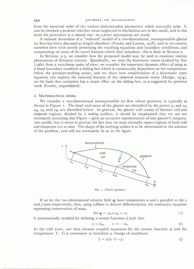
We consider a two-dimensional incompressible ice flow whose geometry is typically as shown in Figure 1. The head and snout of the glacier are identified by the points Xo and Xs; xQ, Xz, and XM are identified below. In general, the glacier will consist of distinct cold and temperate regions, divided by a melting surface; it should be emphasized that we are not necessarily assuming that Figure I gives an accurate representation of every glacier' s tempera­ture profile, but it serves to portray the fact that we must normally expect regions of both cold and temperate ice to exist. The shape of the melting surface is to be determined in the solution of the problem, and will not necessarily be as in the figure.

accumulation

, 1 *

Fig. I. Glacier geometry.

If we let the two-dimensional velocity field q have components u and v parallel to the x and y axes respectively, then, using suffixes to denote differentiation, the continuity equation expressing conservation of mass,

div q = ux+Vy = 0, ( I) is automatically satisfied by defining a stream function rp such that

u = rpy, v = -rpx. (2 ) In the cold zone, one then obtains coupled equations for the stream function <f and the temperature T. It is convenient to introduce a change of coordinate

g = 'rJ(x, t) -y, (3)

RATIONAL MODEL OF A POLYT HERMAL GLACIER 445

where y = 'T](x, t) is the equation of the top surface of the glacier, so g measures the distance downwards from the top surface, and an associated change of variable

x

'Y = 1+:t f H dx,

Xo

where H(x, t) is the depth (measured perpendicular to the x-axis). In a shallow, shearing flow such as in a glacier, the constitutive relation between the strain-rate tensor eij and the stress tensor tij is approximated by the same relation between the shear strain-rate Uy = 1yy = 'Y ss' and the shear stress 72. Since the surface shear stress is approximately zero, the balance between 72y and gravity implies that 72 is proportional to the vertical coordinate g; when the variables are non-dimensionalized, scaled, and reduced (by setting certain small parameters equal to zero), the usual Glen's law for ice with exponent n may be written in the approximate form

'Yss = gn exp (KT). The energy equation is similarly found to be

Tt+'YxTs-'YsTx = f3Ign+I exp (KT)+f32TH'

(5)

(6)

where the left-hand side is the convective derivative (= Tt+uTx+vTy), and the two terms on the right represent the viscous dissipation (strain-rate times stress) and heat conduction (the vertical component of which dominates the horizontal component due to the shallowness of the flow).

The conditions that we impose for these equations on the boundary of the cold zone are:

(i) on the top surface, the surface accumulation/ablation rate and temperature are prescribed;

(ii) on the melting surface, the temperature is equal to the pressure-melting point, and the heat flux is continuous;

(iii) on the (unknown) base, a geothermal heat flux is specified, the normal velocity is zero, and the tangential velocity is a prescribed function of the basal stress and the temperature.

If we define the surface-flux function s(x, t) by x

s(x, t) = f a(x, t) dx,

Xo

where a is the accumulation/ablation rate (a > 0 in the accumulation area, a < 0 in the ablation zone), then the kinematic boundary condition at the top surface requires

v = 'T]t+u1)x-sx ony = 1). (8)

When this is transformed using Equations ('2), (3), and (4) we find

'Y = s(x, t) on g = 0, (9)

where we may define 'Y to be zero at Xo. We also require that

on g = o. ( 10) On the melting surface, scaling shows that the melting temperature is effectively constant (equal to zero when normalized) and if we assume there is no heat flux into the temperate ice by moisture transport away from the melting surface, suitable conditions there are

T = Ts = 0 on g = gM(X, t) (the melting surface). ( I I )

JOUR NAL OF GLACIOLO GY

On the bedrock g = H(x, t ) , the no-flow-through condition implies that g = H is a stream­line, if; = 0 there, that is, using Equation (4) ,

x

'¥= :t f H(cr, t ) dcr

xo{t) on g = H(x, t ) .

A sliding law for the horizontal velocity u = .py = - 'Y!: which is dependent on temperature T and basal stress � H (the depth) is

'¥!; = -F [H, T] on g = H(x, t ) . (13)

Lastly, with zero geothermal heat flux (from scaling considerations) , the heat flux into the cold ice above is equal to the viscous heating generated by basal sliding: this implies

f3zTf,+f3IH'¥f, = 0 for x < Xz, g = H(x, t), (14a)

which is valid until Xz where the basal temperature reaches melting point, beyond which the appropriate condition is

T = 0 for Xz < x < XM, g = H(x, t). (14b)

The approximations (and their physical interpretation) on which these equations are based are discussed below.

The above equations and boundary conditions are not relevant in zones of temperate ice: in these the temperature is effectively constant (T � o°C) and the role of enthalpy variable is taken on by the moisture content (Lliboutry, 1976). It appears that the flow law of temperate ice also depends on the moisture content, and so the equations for '¥ and the moisture content ware once again coupled. In this case it becomes necessary to specify a term in the energy equation which describes the hydrological flow of moisture through the ice (this plays a similar role to that of heat conduction in cold ice) . It is clear that a proper description of such a term is necessary before the dynamics of temperate ice can be usefully studied. In the earlier paper (Fowler and Larson, 1978), it was assumed, for want of any better information, that the transport by this means was negligible; in this case the cold zone effectively uncouples from the solution in the temperate zone, and the latter is of little further interest: subsequent analysis is then largely concerned with the cold zone-or with completely polar glaciers.

It will be noticed in Equation (13) that the sliding law is taken to be a function not only of the basal stress (�H) but also of the temperature T: this is to accommodate the realistic physics (Fowler, 1979) which demands that the basal velocity should increase from zero to its full temperate value over a small (typically IO-I deg) but crucially finite temperature range just below the pressure-melting point: the important consequence of this novel assumption is discussed below in Section 4. The points XQ, Xz, XM in Figure 1 and in Equation (14) may now be interpreted as follows: XQ is the point where the basal ice first begins to slide ; the ice is wholly frozen to the bedrock in (xo, xQ). The point Xz is where the temperature reaches melting point and the sliding law is the fully temperate one; thus (xQ' xz) is the region of "sub-temperate" sliding. Lastly, XM is the point where the melting surface on which T = 0 "breaks away" from the bedrock; in (xz, XM) the basal temperature is at the melting point, but the viscous source heating at the boundary is used up in warming the cold ice above until Tf, = 0 (i.e. the heat flux into the ice decreases to zero) which is precisely when x = XM. The melting surface gM dividing cold and temperate ice is a necessary constituent of the model, since in general cold ice will be heated by the frictional dissipation source term in the energy equation. It is however quite realistic to consider particular limits represented by the so-called "polar" and "temperate" glaciers. In view of the comments above on moisture transport, realistic models for the latter cannot be said to exist.

The assumptions made in deriving the reduced model presented above are the following: the Reynolds number (Re) = 0; 0 (typical depth/length) = 0; JL = 8/(mean bedrock

RATIONAL MODEL OF A POLYT HERMAL GLACIER 447

slope) = 0; A (dimensionless geothermal heat flux) = 0; and that Z, which measures the error in assuming an exponential form exp [K T] for the temperature dependence of the flow law rather than the more usual Arrhenius term, is zero. These approximations are based on the numerical estimates

(Re) ;:::: 10-'3, } 8 ;:::: 10-2,

1-', A, Z;:::: 10-'.

The Reynolds number (Re) measures the slowness of the flow, and its neglect entails ignoring inertial terms in the momentum equations; 8 is a measure of the shallowness of the flow; neglecting I-' means that variations of the surface slope from the mean bedrock slope are ignored. (Note that this neglect of I-' is inapplicable to a flow with a horizontal base, e.g. an ice sheet, to which the definition of I-' is not appropriate. ) The above approximations are expected to be good ones, in the sense that they are mostly of non-singular type; this is not strictly true of the neglect of 8 and 1-', but neglect of 8 only appears to be associated with a degeneracy of the equations near the head Xo and snout xs, and does not affect the bulk of the flow. The parameter p. represents a diffusional term for kinematic waves, and thus may become prominent if its neglect leads to the prediction of surface shock waves: for further discussion of this point, see Fowler and Larson (in press).

The important parameters arising in the model are K, f31> and (32' These measure res­pectively the strength of the dependence of viscosity on temperature, the magnitude of the viscous source heating, and the magnitude of heat conduction. With typical values of the physical input parameters, it is found that these parameters are of numerical order one, although with a realistic variation of such quantities as mean accumulation-rate, mean bedrock slope, etc. , larger or smaller values may easily be obtained: in particular, (3, and f32 may be small. Furthermore, when the analogue of Equation (6) is studied for larger ice masses such as ice sheets, it is expected that realistically small values of f32 may be obtained. For these (and purely mathematical) reasons, it is of interest to study the proposed model under various asymptotic limits of the given parameters. In general, this is not an easy task.

3. KINEMATIC WAVES IN THE LIMIT K --+ 0

If we suppose that the surface-flux function s(x, t) is independent of t, that is s(x, t) =s(x) , then on integrating Equation (5) twice and using the boundary conditions for '1", Equations (9), (12), and (1 3), we find that in x < XM conservation of mass takes the form

Ht+Qx = s' (x) ,

where the flux Q is given by H

Q = HUb+ f gn+' exp (KT) dg, ( 17)

o

and Ub = F(H, T) is the basal sliding velocity. Equations of the form of Equation (16) were studied by Lighthill and Whitham (1955) and applied to glacier flow by Weertman (1958) and Nye (1960,196 3), There is a slight subtlety in the present case, since the basic ("datum") steady state is of finite extent, and so linear analyses of the type proposed by ye lead to non­uniformly bounded solutions at the snout, where H --+ o. One can easily avoid this pitfall by applying the method of characteristics to the essentially non-linear system of Equation (16). As an illustration, we suppose x < xQ, that is Ub = 0, and take the formal asymptotic limit K --+ o. In this case we obtain

JOURNAL OF GLACIOLO GY

of which the characteristic equations are

dx - = Hn+, dt '

dH dt = s'(x) .

( 19)

Equation (19) immediately gives the wave speed, which is approximately four times the surface speed (this being Hn+'jn+I). The solution of Equations (19) and (20) may be written down in terms of a characteristic parameter cr E [xo, xs(o)]. It is

Hn+z -

+ = s(x)-s,(cr) , (21 )

n 2

f dx t = Hn+,'

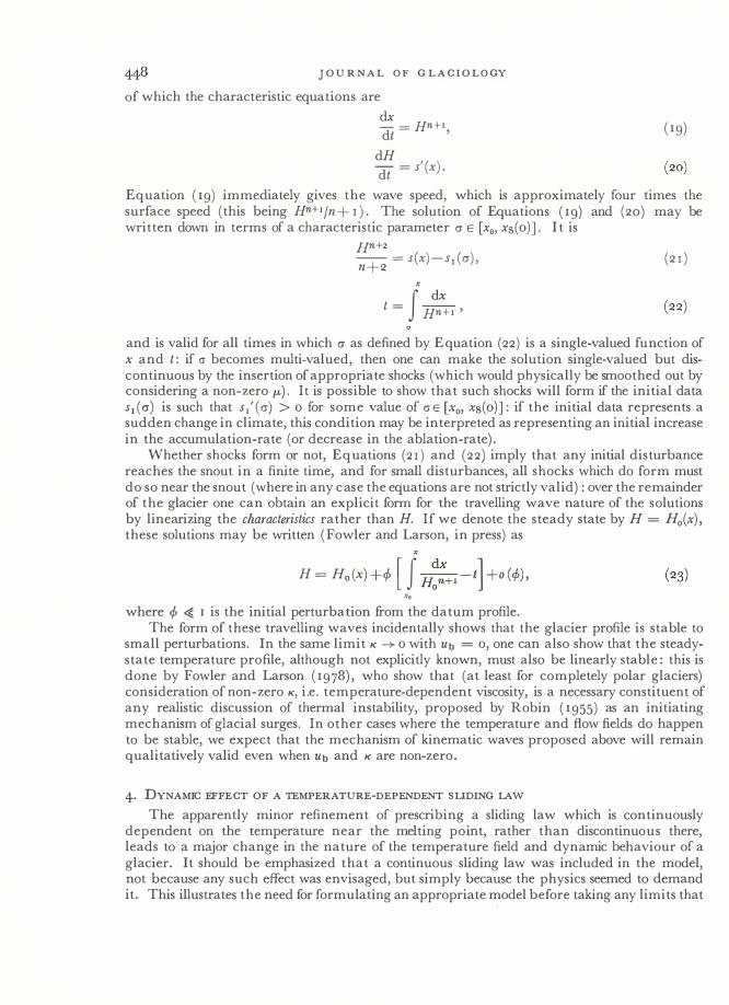
and is valid for all times in which cr as defined by Equation (22) is a single-valued function of x and t: if cr becomes multi-valued, then one can make the solution single-valued but dis­continuous by the insertion of appropriate shocks (which would physically be smoothed out by considering a non-zero fl-). It is possible to show that such shocks will form if the initial data s,(cr) is such that s,' (cr) > 0 for some value of crE [xo, xs(o)]: if the initial data represents a sudden change in climate, this condition may be interpreted as representing an initial increase in the accumulation-rate (or decrease in the ablation-rate).

Whether shocks form or not, Equations (21) and (22) imply that any initial disturbance reaches the snout in a finite time, and for small disturbances, all shocks which do form must do so near the snout (where in any case the equations are not strictly valid) : over the remainder of the glacier one can obtain an explicit form for the travelling wave nature of the solutions by linearizing the characteristics rather than H. If we denote the steady state by H = Ho(x), these solutions may be written (Fowler and Larson, in press) as

x

H = Ho(x) +c/> [f H�:+I -t] +0 (c/», '0

where c/> <{ I is the initial perturbation from the datum profile. The form of these travelling waves incidentally shows that the glacier profile is stable to

small perturbations. In the same limit K -+ 0 with Ub = 0, one can also show that the steady­state temperature profile, although not explicitly known, must also be linearly stable : this is done by Fowler and Larson (1978), who show that (at least for completely polar glaciers) consideration of non-zero K, i.e. temperature-dependent viscosity, is a necessary constituent of any realistic discussion of thermal instability, proposed by Robin (1955) as an initiating mechanism of glacial surges. In other cases where the temperature and flow fields do happen to be stable, we expect that the mechanism of kinematic waves proposed above will remain qualitatively valid even when Ub and K are non-zero.

4. DYNAMIC EFFECT OF A TEM PERATURE-DE PENDENT SLIDING LAW

The apparently minor refinement of prescribing a sliding law which is continuously dependent on the temperature near the melting point, rather than discontinuous there, leads to a major change in the nature of the temperature field and dynamic behaviour of a glacier. It should be emphasized that a continuous sliding law was included in the model, not because any such effect was envisaged, but simply because the physics seemed to demand it. This illustrates the need for formulating an appropriate model before taking any limits that

RAT IONAL MODEL OF A POLYTHERMAL GLACIER 449

suggest themselves, since in this case it is found that the limiting behaviour of a glacier as the sliding law becomes discontinuous is not the same as that of a glacier with a discontinuous sliding law. Such non-uniform limits are commonly encountered in other areas of applied mathematics; in the present case the above discrepancy occurs because the discontinuous sliding law has a finite jump at T = 0 and no intermediate basal velocity between 0 and F [H, 0] is possible, whereas in the limiting form of the continuous law, any such intermediate velocity is admissible at T = 0, and thus the discontinuous law does not really represent the correct limit of the continuous law. More specifically, if we admit a discontinuous sliding law of the form

Ub = F(H), T=o,

w=o, } w > o,

Ub = 0, T<o,

then, since the basal velocity is discontinuous, there must be some kind of discontinuity in the surface behaviour, and if f.L = 0, this takes the form of a finite jump in the depth at the point XQ (= Xz in this case). Now if we examine the particular asymptotic limit of the steady-state versions of the model given by Equations (5) and (6) in which f32 -+ 00 with f3d f32 finite (admittedly this is unlikely to be a realistic case), it is found that just as for K = 0, the equations uncouple (the convective terms vanish) and the solution for the entire problem in the cold zone may be constructed from a knowledge of the temperature, which may be found explicitly as the solution of a second-order differential equation in g which is parametrically dependent on x through the boundary data on g = 0 and g = H. It is then found from this explicit solution that if ( -v, 0) is the dimensionless temperature range over which the sliding velocity increases from zero to its full temperate value, i.e. T = -vat XQ and T = 0 at Xz, then in the limit as v -+ 0, xQ -H Xz, and so the glacier behaviour with v = 0 is not the same as that when v -+ o. A reasonable estimate for v is 10-2, so we see that v is indeed small. From the above result, it is clear that rather than apply the boundary condition Ub = F[H, T] in (xQ' xz) , we should in the limit v -+ 0 specify that T = 0 there. Thus the effective boundary conditions to replace Equations (13) and (14) are

'Y, = 0, f31H'¥S+f32TS = 0,

T=o, 'Ys = -F[H, 0],

x < xQ, x < Xz,

xQ < x < XM , Xz < X < XM, }

and we see that there are three separate sets of boundary conditions to be applied on g = H. Equation (25) is the correct limiting version of Equation (13) ; it obviates the need to specify F [H, T] for T < 0 , which is just as well, and it is fairly clear that a numerical solution of the equations will be much simpler with these effective boundary conditions. Questions of stability are slightly more subtle. These are to be discussed in a paper in preparation by A. C. Fowler and D. A. Larson.

What happens in (xQ, xz) is clear: the basal velocity is essentially governed by the bulk ice flow rather than the basal "inner flow" (which really specifies the precise basal tempera­ture in ( -v, 0)), and Ub gradually increases in (xQ, xz) until it becomes equal to the full sliding velocity F(H, 0). Thus we must expect that, in general, glaciers may have substantial parts of their bases at temperatures within this "sub-temperate" range, and accordingly basal velocities within these regions will not appear to be functionally related to the basal stress (and hence the depth). Although this result is explicitly derived in the particular limit f32 -+ 00, it depends only on the continuity of the sliding law, and hence will be valid for any value of f32 whatsoever, as long as v � I. This result in itself justifies the study of the limit f32 -+ 00, and answers negatively the question posed by Robin's (1976) paper-at least in certain regions.

JOURNAL OF GLACIOLOGY

5. SEASONAL WAVES

Seasonal waves are waves of velocity disturbances which propagate at very high speeds down glaciers (typically 20 to 150 times the surface speed). They have been reported by, amongst others, Deeley and Parr (1914) on Hintereisferner and Hodge (1974), who observed such waves on Nisqually Glacier with an approximate speed of 20 km a-I.

To date, no satisfactory theoretical explanation of their behaviour has been forthcoming. Weertman (1962) considered the effect of kinematic waves in the subglacial water film, while Hodge (1974) considered that the waves might be due to a correlation between the sliding velocity and the liquid water stored in the glacier, since the latter varies on a seasonal basis. While this may be an important part of the phenomenon, it does not in itself answer the fundamental question: why are the wave propagation speeds so large? And why do the waves consist of velocity perturbations with no apparently related wave motions in the depth?

One possible answer to these questions is provided below. We will essentially concentrate on Hodge's paper, and in particular seek to understand his figure 6, which is a contour map in (x, t) space of the surface velocity. The lines of constant velocity mostly oscillate in space, but some form closed loops: the contours are skewed slightly, which represents a seasonal wave with a transit time of about a month from the equilibrium line to the snout.

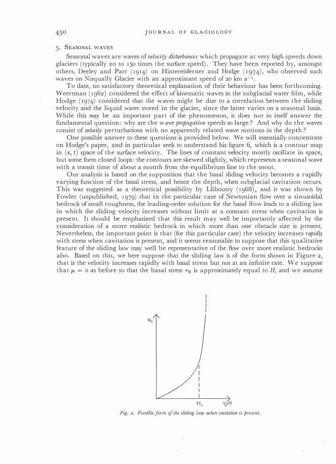
Our analysis is based on the supposition that the basal sliding velocity becomes a rapidly varying function of the basal stress, and hence the depth, when subglacial cavitation occurs. This was suggested as a theoretical possibility by Lliboutry (1968), and it was shown by Fowler (unpublished, 1979) that in the particular case of Newtonian flow over a sinusoidal bedrock of small roughness, the leading-order solution for the basal flow leads to a sliding law in which the sliding velocity increases without limit at a constant stress when cavitation is present. It should be emphasized that this result may well be importantly affected by the consideration of a more realistic bedrock in which more than one obstacle size is present. Nevertheless, the important point is that (for this particular case) the velocity increases rapidly with stress when cavitation is present, and it seems reasonable to suppose that this qualitative feature of the sliding law may well be representative of the flow over more realistic bedrocks also. Based on this, we here suppose that the sliding law is of the form shown in Figure 2, that is the velocity increases rapidly with basal stress but not at an infinite rate. We suppose that J.L = 0 as before so that the basal stress Tb is approximately equal to H, and w e assume

He TJi'H

Fig. 2. Possible form of the sliding law when cavitation is present.

RATIONAL MODEL OF A POLYTHER M AL GLACIER 451

cavitation sets in when H � Hc. We will formally assume that shearing within the ice mass is negligible, so that the flux

Q � UbH, (26)

and Q increases rapidly near Hc. (This assumption is not necessary for the subsequent analysis.) The kinematic wave equation describing conservation of mass is then

Ht+Qx = s'(x) , (27)

if we suppose that the flux function s is independent of time. The steady-state solution of Equation (27) is

Q = s(x) .

If we denote the critical value of Q at Hc by Qc, then in regions where Qc < s(x) , the glacier will be of effectively constant depth Hc. In such regions, a small perturbation in the depth will generally have a large effect on Q (and hence the surface velocity) .

Now the characteristic equations (see, e.g. Whitham, 1974) of Equation (27) may be written as

dx

dt = Q'(H) ,

dH - = s'(x) . dt

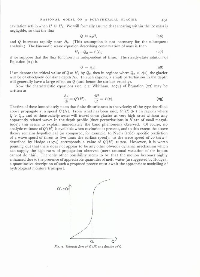
The first of these immediately states that finite disturbances in the velocity of the type described above propagate at a speed Q'(H) . From what has been said, Q'(H) � I in regions where Q > Qc, and so these velocity waves will travel down glacier at very high rates without any apparently related waves in the depth profile (since perturbations in H are of small magni­tude) : this seems to explain immediately the basic phenomena observed. Of course, no analytic estimate of Q' (H) is available when cavitation is present, and to this extent the above theory remains hypothetical (as compared, for example, to Nye's (1960) specific prediction of a wave speed of three to five times the surface speed) : to the wave speed of 20 km a-I described by Hodge (1974) corresponds a value of Q' (H) � 200. However, it is worth pointing out that there does not appear to be any other obvious dynamic mechanism which can supply the high rates of propagation observed (mere seasonal variation of the inputs cannot do this) . The only other possibility seems to be that the motion becomes highly enhanced due to the presence of appreciable quantities of melt water (as suggested by Hodge) : a quantitative description of such a proposed process must await the appropriate modelling of hydrological moisture transport.

Qc Q Fig. 3. Schematic form of Q'(H) as a function of Q.

452 JOURNAL OF GLACIOLOGY

If we write Q'(H) as a function of Q, say

Q' = c(Q), (30)

then we see from Figure 2 that c( Q) will have the form shown in Figure 3, with critical behaviour at Q = Qc. Multiplying Equation (27) by Q'(H) == c(Q), we obtain the wave equation for the flux in the form

Qt+c( Q) Qx = s' (x) c( Q). For regions in which Q > Qc, we have by assumption

c(Q) � I.

If we define a small parameter E by considering c(Q) � I/E, and let

t = E'T, } c(Q) = � C(Q),

then the correctly scaled version of Equation (31) is

Q�+c(Q) Qx = s'(x) C(Q), (34)

valid for the description of se�sonal waves over the fast time scale 'T. Equation (34) is applicable in regions where s(x) > Qc. Denote such a region by (XI' x2), and suppose s(x) < Qc outside this region. In the limit as E --+ 0, we require that flux changes outside (XI' x2) should occur over the longer convective time scale t, and so appropriate conditions on Q are that Q = Qc at XI and X2• We can satisfy the up-stream boundary condition at XI> but not in general the second: this may require the reintroduction of the diffusion-like coefficient IL, which would correspondingly introduce a small term proportional to Qxx in Equation (34), and an associated local analysis in the vicinity of x2; we shall not consider this subtlety further in the present instance.

For want of any better information, we now choose

C(Q) = I, to illustrate the sort of behaviour we expect. For Nisqually Glacier, a typical value of E is 5 X 10-3: the bulk-flow time scale may be estimated at 20 years, so that this lE corresponds to a transit time down-glacier of c. 1 month (as observed). With Equation (35), Equation (34) is

with solution

Q = s(x) +c/>(x-'T), (37) where c/> represents a travelling wave generated by an initial disturbance c/>(x), c/>(xI) = o. Let us now seek the solution corresponding to a regular variation in the flux function. Like Fowler and Larson (in press), we model such a seasonal variation by adding a sinusoidal term to s(x), and thus seek solutions of

Q�+Qx = s'(x) +s/(x) exp (i.Q'T), (38)

where the real part of Q is to be taken. With E � 5 X 10-3 and t associated with a time scale of 20 years, 'T is associated with a scale

of c. I month; the seasonal variation defined by Equation (38) has a dimensionless period (in 'T) of 27T/.Q � 6/0.: since this corresponds to 1 year = 12 months, we have 6/0. � 12, i.e. apparently 0. � t for Nisqually Glacier. Typically we may take 0. � I. (Contrast the effect of seasonal variation on Nye's kinematic waves, where the seasonal frequency relative to the long time scale is so fast that its effect is "averaged out" and may be neglected (Fowler and Larson, in press).)

RAT IONAL MODEL OF A POLYTHERMAL GLACIER 45 3

The solution of Equation (38) is (if we impose Q = s(x) at XI)' x

Q = s(x)+exp [i.o(T-x)] f s/(x) exp (i!1x) dx.

Since .0 � I, Equation ( 39) represents a regular seasonal wave of finite amplitude (if s / = 0 ( I)). To be more specific, let us choose

s/ = a > 0,

where a is constant. Equation (40) reflects a steady oscillation between extra accumulation and ablation: realistically we expect a � I. We then find, on substituting Equation (40) into Equation ( 39), evaluating and taking the real part of the resultant expression, that

Q = s(x) + � sin (�x) cos { .0 (T-;)} = s(x)+� [sin !1T+sin {.o(X-T)}],

where for convenience we choose XI = o. Thus Q may b e thought of as a modulated wave of speed 2, or as a travelling wave of constant shape and speed 1 together with a superimposed oscillatory component. Hodge (1974) gives data on a relationship of this type in the form (his fig. 6) of a contour map of the surface velocity in the (t, x) plane. We may obtain the charac­teristic features of such a map in the present case by writing

.ox X = -, T = .oT, (42) 2

and seeking intersections in the (T, X) plane of the two surfaces

ZI = sin X cos (T -X), and

for various different (constant) values of Q (corresponding to different values of the surface velocity). The surface described by Equation (44) is a smooth sheet which, for reasonable functions s bends concavely upwards in the X direction (if we suppose XI lies in the ablation zone). On the other hand, sin X cos T represents an "egg-box" curve in the (T, X) plane consisting of a checkered formation of undulating peaks and troughs. Changing this to sin X cos (T -X) simply has the effect of skewing the undulations in the T direction, but does not materially alter the properties of the intersection of Equations (43) and (44). The inter­section determines two types of curves depending on the value of Q. As T -X increases from zero on curve ( I) in Figure 4a, the locus of the intersection which lies on the point El on the peak (solid line) decreases in X; hence Zz decreases until Zz = 0 when the locus leaves the peak and enters the trough, the axis of which is the dotted line in the figure at T -X = 'TT. X further decreases till the point AI is reached at T -X = 'TT, after which the locus retraces its steps to BI at T -X = 2 'TT. Thus the locus is an oscillating curve in (X, T -X) space.

The same is true of the locus bounded by the points Az and Bz on curve (2) in Figure 4a. However, that bounded by M and N consists of a series of closed loops, because these loci cannot leave the peaks on which they lie, since MN does not cross the X axis. The curves bounded b y MN, AzBz, and AIBI are shown from top t o bottom in Figure 4b, and one can immediately note the resemblance to figure 6 of Hodge (1974): however, there are also striking differences, and one should not attempt to seek too great a quantitative comparison.

454

x

JOURNAL O F GLACIOLOGY

(1) (2)

(a)

smaller /

/

/1° // 0 ///

/ /

/ /

(b) Fig. 4.

/ / /

/

/ /

/ /

x

a. Sectional view of intersection of the two curves representing Equations (43) and (44). b. Possible form of contours Q = constant in the (T, X) plane.

An alternative way of examining Equation (41) in relation to this figure is to consider the "height" Q to be the superimposition of the decreasing function s(x) and the skewed egg-box. The overall "topography" is then that of a slope downwards to the snout x = Xs, with various hills and basins evident due to the seasonal variation: again this is essentially what is repre­sented in Hodge's figure. Of course the present model is a huge simplification of any realistic seasonal waves, and cannot be used for predictive purposes (at least not quantitatively) . Even so, there are two particular facets of the above explanation that must be considered in terms of the qualitative applicability of the theory. One is that a much larger value ofQ than that given here ( � t) must be invoked in order to obtain the secondary "loops" evident in Hodge's figure: this is probably not very important in view of the quantitative assumptions of the model. Of more importance is any possible discrepancy between the phase of the level curves in Equation (41a) and in Hodge's diagram, since as he says, "the acceleration �rthe glacier throughout the winter in the ablation zone is crucial to a correct interpretation of the velocity variations". It is therefore important to try and relate the phase of Equation (41a) to that of the experi­mental data. We see that sin tQx is a maximum when x = 7TjQ. At this point

Q = s(x) + � cos { Q (T-2�) } = s(x) + � sin QT.

RATIONAL MODEL OF A POLYTHER MAL GLAC IER 455

Now we see from Equations (38) and (40) that the variation in the seasonal accumulation-rate is a cos rh, so that the origin T = 0 corresponds to the time of maximum accumulation-rate, i.e. winter. On examining Hodge's figure 6, it seems that in the above context, a suitable choice of "x = 7TjQ" is about 300-400 m along the centre line, and here the Q profile in T is indeed "sinusoidal" with the origin taken about February. It is hard to be more specific, but this seems to agree to a reasonable extent with the theory. (It is difficult for example to say where the origin x = 0 at which the waves are initiated should be put.)

More detailed analysis is necessary to determine whether such apparent phase agreement is adequate to explain the observed results: this is rather important in view of Hodge's idea that liquid water storage, in particular at the glacier base, may have a major effect on the dynamics of temperate glaciers.

Lastly we consider Hodge's figure 13, in which the surface speed averaged over 19 roughly equally spaced x-positions is plotted against time. We compare this with taking the average in x of Q as defined by Equation (41 b) , with the assumption that x = Xs is close to a period of sin Qx. The result is (denoting averages by overbars)

_ a . Q = s+Q

sm QT,

which is very similar to the second graph in Hodge's figure 13 for 1969, if we choose an origin T = 0 at about March. This is again suggestive rather than predictive, but the agreement is nevertheless quite satisfactory.

REFERENCES

Deeley, R. M., and Parr, P. H. 1914. On the Hintereis Glacier. Philosophical Magazine, Sixth Ser., Vo!. 27, No. 157, p. 153-76.

Fowler, A. C. 1979. A mathematical approach to the theory of glacier sliding. Journal of Glaciology, Vo!. 23, No. 89, p. 131-41.

Fowler, A. C. Unpublished. Glacier dynamics. [D.Phi!. thesis, University of O xford, 1977.] Fowler, A. C., and Larson, D. A. 1978. On the flow of poly thermal glaciers. Part I: model and preliminary

analysis. Proceedings of the Royal Society of London, Ser. A, Vo!. 363, No. 1713, p. 2 I 7-42. Fowler, A. C., and Larson, D. A. In press. On the flow of poly thermal glaciers. Part 11: surface wave analysis.

Proceedings of the Royal Society of London, Ser. A. Glen, ]. W. 1955. The creep of polycrystalline ice. Proceedings of the Royal Society of London, Ser. A, Vo!. 228,

No. 1175, p. 519-38. Hodge, S. M. 1974. Variations in the sliding of a temperate glacier. Joumal of Glaciology, Vo!. 13, No. 69,

P·349-69· Lighthill, M. ]., and Whitham, G. B. 1955. On kinematic waves. Proceedings of the Royal Society of London, Ser. A,

Vo!' 229, No. I I 78, p. 281-345. Lliboutry, L. A. 1968. General theory of subglacial cavitation and sliding of temperate glaciers. Journal of

Glaciology, Vo!. 7, No. 49, p. 21-58. Lliboutry, L. A. 1976. Physical processes in temperate glaciers. Journal of Glaciology, Vo!. 16, No. 74, p. 151-58. Nye, ]. F. 1960. The response of glaciers and ice-sheets to seasonal and climatic changes. Proceedings of the Royal

Society of London, Ser. A, Vo!. 256, No. 1287, p. 559-84. Nye, ]. F. 1963. The response of a glacier to changes in the rate of nourishment and wastage. Proceedings of the

Royal Society of London, Ser. A, Vo!. 275, No. 1360, p. 87-1 12. Robin, G. de Q. 1955. Ice movement and temperature distribution in glaciers and ice sheets. Joumal ofGlaciology,

Vo!. 2, No. 18, p. 523-32. Robin, G. de Q. 1976. Is the basal ice of a temperate glacier at the pressure melting point? Joumal of Glaciology,

Vo!. 16, No. 74, p. 183--96. Weertman, ]. 1958. Traveling waves on glaciers. Union Geodesique et GeoPhysique Intemationale. Association Inter­

nationale d'Hydrologie Scientifique. Symposium de Chamonix, I6--24 sept. I958, p. 162-68. (Publication No. 47 de l'Association Internationale d'Hydrologie Scientifique )

.

Weertman, ] 1962. Catastrophic glacier advances. Union Geodisique et Geophysique Intemationale. Association Intemationale d'Hydrologie Scentifique. Commission des Neiges et des Glaces. Col/oque d'Obergurgl, Io--!}-18-9 1962, p. 31-39. (Publication No. 58 de I'Association Internationale d'Hydrologie Scientifique.)

Whit ham, G. B. 1974. Linear and non-linear waves. New York, Wiley-Interscience.

JOURNAL OF GLACIOLOGY

DISCUSSION

G. K. C. CLARKE : I hope you did not mean to imply that a discontinuity in the sliding law would demand a discontinuity in thickness at the boundary between frozen and unfrozen bed. Real glaciers would not have this problem.

A. C. FOWLER: Mathematically, a discontinuity would occur if S = fA- = 0, that is the smooth­ing terms represented by surface-slope variations and longitudinal stress were neglected. Physically, these terms would indeed be able to smooth the discontinuity, but I do not think this alters the conclusion about "sub-temperate" basal regions.

A. IKEN: Measurements of ice temperature in cold glaciers have shown that the warmest ice is found in that part of the accumulation area where melt water percolates into the snow. In some zone down-glacier, in the ablation area, the ice temperature is colder. Warming up of the ice due to energy dissipation in shearing is concentrated in a region near the bed. I would like to suggest that you take into account, in your model, the principal temperature distribution as it is indicated by measurements.

FOWLER: On the second point, the importance of basal shear heating is, of course, intrinsically represented in the model by the size of the various dimensionless parameters, in particular that representing viscous dissipation (f1,). Variations of temperature in the accumulation area of the kind you describe would be due to a particular type of imposed surface temperature, which can also be considered as included in the boundary conditions.

The aim of modelling is to describe the essential physical processes, and comparison with observations should not be artificially introduced.